Deep convolutional tensor network

Abstract

Neural networks have achieved state of the art results in many areas, supposedly due to parameter sharing, locality, and depth. Tensor networks (TNs) are linear algebraic representations of quantum many-body states based on their entanglement structure. TNs have found use in machine learning. We devise a novel TN based model called Deep convolutional tensor network (DCTN) for image classification, which has parameter sharing, locality, and depth. It is based on the Entangled plaquette states (EPS) TN. We show how EPS can be implemented as a backpropagatable layer. We test DCTN on MNIST, FashionMNIST, and CIFAR10 datasets. A shallow DCTN performs well on MNIST and FashionMNIST and has a small parameter count. Unfortunately, depth increases overfitting and thus decreases test accuracy. Also, DCTN of any depth performs badly on CIFAR10 due to overfitting. It is to be determined why. We discuss how the hyperparameters of DCTN affect its training and overfitting.

1 Introduction

1.1 Properties of successful neural networks

Nowadays, neural networks (NNs) achieve outstanding results in many machine learning tasks [21], including computer vision, language modeling, game playing (e.g. Checkers, Go), automated theorem proving [23]. There are three properties many (but not all) NNs enjoy, which are thought to be responsible for their success. For example, [7] discusses the importance of these properties for deep CNNs.

• Parameter sharing, aka applying the same transformation multiple times in parallel or sequentially. A layer of a convolutional neural network (CNN) applies the same function, defined by a convolution kernel, to all sliding windows of an input. A recurrent neural network (RNN) applies the same function to the input token and the hidden state at each time step. A self-attention layer in a transformer applies the same query-producing, the same key-producing, and the same value-producing function to each token. [1]

• Locality. Interactions between nearby parts of an input are modeled more accurately, while interactions between far away parts are modeled less accurately or not modeled at all. This property makes sense only for some types of input. For images, this is similar to receptive fields in a human’s visual cortex. For natural language, nearby tokens are usually more related than tokens far away from each other. CNNs and RNNs enjoy this property.

• Depth. Most successful NNs, including CNNs and transformers, are deep, which allows them to learn complicated transformations.

1.2 The same properties in tensor networks

Tensor networks (TNs) are linear algebraic representations of quantum many-body states based on their entanglement structure. They’ve found applications in signal processing. People are exploring their applications to machine learning, e.g. tensor regression – a class of machine learning models based on contracting (connecting the edges) an input tensor with a parametrized TN. Since NNs with the three properties mentioned in Section 1.1 are so successful, it would make sense to try to devise a tensor regression model with the same properties. That is what we do in our paper. As far as we know, some existing tensor networks have one or two out of the three properties, but none have all three.

• MERA (see Ch. 7 of [4]) is a tree-like tensor network used in quantum many-body physics. It’s deep and has locality.

• Deep Boltzmann machine can be viewed as a tensor network. (See Sec. 4.2 of [5] or [9] for discussion of how restricted Boltzmann machine is actually a tensor network. It’s not difficult to see a DBM is a tensor network as well). For supervised learning, it can be viewed as tensor regression with depth, but without locality or weight sharing.

• [9] introduced Entangled plaquette states (EPS) with weight sharing for tensor regression. They combined one EPS with a linear classifier or a matrix tensor train. Such a model has locality and parameter sharing but isn’t deep.

• [7] introduced a tensor regression model called Deep convolutional arithmetic circuit. However, they used it only theoretically to analyze the expressivity of deep CNNs and compare it with the expressivity of tensor regression with tensor in CP format (canonical polyadic / CANDECOMP PARAFAC). Their main result is a theorem about the typical canonical rank of a tensor network used in Deep convolutional arithmetic circuit. The tensor network is very similar to the model we propose, with a few small modifications. We conjecture that the proof of their result about the typical canonical rank being exponentially large can be modified to apply to our tensor network as well.

• [18] did language modeling by contracting an input sequence with a matrix tensor train with all cores equal to each other. It has locality and parameter sharing.

• [16] used a tree-like tensor regression model with all cores being unitary. Their model has locality and depth, but no weight sharing.

• [25] and [19] performed tensor regression on MNIST images and tabular datasets, respectively. They encoded input data as rank-one tensors like we do in Section 3.1 and contracted it with a matrix tensor train to get predictions. Such a model has locality if you order the matrix tensor train cores in the right way.

1.3 Contributions

The main contributions of our article are:

• We devise a novel tensor regression model called Deep convolutional tensor network (DCTN). It has all three properties listed in Section 1.1. It is based on the (functional) composition of TNs called Entangled plaquette state (EPS). DCTN is similar to a deep CNN. We apply it to image classification, because that’s the most straightforward application of deep CNNs. (Section 3.3)

• We show how EPS can be implemented as a backpropagatable function/layer which can be used in neural networks or other backpropagation based models (Section 3.2).

• Using common techniques for training deep neural networks, we train and evaluate DCTN on MNIST, FashionMNIST, and CIFAR10 datasets. A shallow model based on one EPS works well on MNIST and FashionMNIST and has a small parameter count. Unfortunately, increasing depth of DCTN by adding more EPSes hurts its accuracy by increasing overfitting. Also, our model works very badly on CIFAR10 regardless of depth. We discuss hypotheses why this is the case. (Section 4).

• We show how various hyperparameters affect the model’s optimization and generalization (Appendix A).

2 Notation

An order-$N$ tensor is a real valued multidimensional array $A\in\mathbb{R}^{I_{1}\times\dots\times I_{N}}$. A scalar is an order-0 tensor, a vector is an order-1 tensor, a matrix is an order-2 tensor. We refer to a slice of a tensor using parentheses, e.g. $A(i_{1},\dots,i_{k})\in\mathbb{R}^{I_{k+1}\times\dots\times I_{N}}$, $A(i_{1},\dots,i_{N})\in\mathbb{R}$. In the second case we got a scalar, because we fixed all indices. We can vectorize a tensor to get $\operatorname{vec}(A)\in\mathbb{R}^{I_{1}\cdots I_{N}}$. If a tensor has order at least 2, we can separate its dimensions into two disjoint sets $L\sqcup R=\{I_{1},\dots,I_{N}\}$ and matricize the tensor, i.e. turn it into an $\prod_{I\in L}I$ by $\prod_{I\in R}I$ matrix $\operatorname{mat}(A)$. When we use matricization, we won’t explicitly specify how we separate the dimensions into disjoint sets, because it should be clear from context. If we also have a tensor $B\in\mathbb{R}^{J_{1}\times\dots\times J_{M}}$, their outer product $A\otimes B\in\mathbb{R}^{I_{1}\times\dots\times I_{N}\times J_{1}\times\dots\times J_{M}}$ is defined as

$$(A\otimes B)(i_{1},\dots,i_{N},j_{1},\dots,j_{M})=A(i_{1},\dots,i_{N})B(j_{1},\dots,j_{M}).$$

If, in addition to $A$, for some $n\in\{1,\dots,N\}$ we have a vector $x\in\mathbb{R}^{I_{n}}$, we can contract them on the $n$-th dimension of $A$ to produce an order-$(N-1)$ tensor $A\operatorname{\bar{\times}}_{n}x\in\mathbb{R}^{I_{1}\times\dots\times I_{n-1}\times I_{n+1}\times I_{N}}$ defined as

$$(A\operatorname{\bar{\times}}_{n}x)(i_{1},\dots,i_{n-1},i_{n+1},\dots,i_{N})=\sum_{i_{n}=1}^{I_{n}}A(i_{1},\dots,i_{n-1},i_{n},i_{n+1},\dots,i_{N})x(i_{n}).$$

Contraction can also be performed between a tensor and a tensor. However, to denote this we use TN diagrams instead of formulas – see Figure 1.

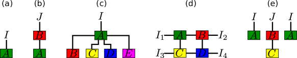
Figure 1: (a) Vector $A\in\mathbb{R}^{I}$. (b) Matrix-vector product $BA=B\operatorname{\bar{\times}}_{2}A\in\mathbb{R}^{J}$. (c) Contraction of an order-5 tensor $A$ with 4 vectors $B,C,D,E$ results in vector $A\operatorname{\bar{\times}}_{5}E\operatorname{\bar{\times}}_{4}D\operatorname{\bar{\times}}_{3}C\operatorname{\bar{\times}}_{2}B\in\mathbb{R}^{I}$. (d) Contraction of four order-3 tensors, which results in an order-4 tensor. (e) Traditionally, if a TN diagram contains disconnected subgraphs, the whole diagram represents their outer product $A\otimes BC\otimes A\in\mathbb{R}^{I\times J\times I}$. However, in our work, we usually interpret it as simply a collection of tensors $(A,BC,A)$.

There are multiple introductions to TN diagrams available. We recommend Chapter 1 of [4], [8] (this article doesn’t call them TNs, but they are), and Chapter 2 of [6]. Other introductions, which are less accessible for machine learning practitioners, are [20] and [3].

We extend the notion of TNs by introducing the copy operation. We call tensor networks with the copy operation generalized TNs. The copy operation was invented by [9]. It takes a vector as input and outputs multiple copies of that vector. In generalized TN diagrams, we graphically depict the copy operation by a red dot with one input edge marked with an arrow, and all output edges not marked in any way. This operation is equivalent to having multiple copies of the input contracted with the rest of the tensor network. In order for a generalized tensor network to be well defined, it must have no directed cycles going through copy elements (if we consider the usual edges between tensors to have both directions). Figure 2 explains the copy operation in more detail.

(a)

(b)

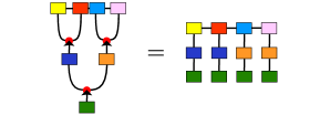
(c)

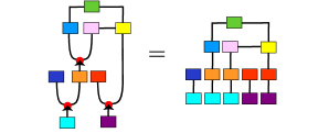
(d)

(e)

Figure 2: (a) Copy operation of a vector input $A$. The result can be interpreted either as the matrix $A\otimes A$ or as just a collection of two vectors $(A,A)$. (b), (c) and (d) : Mapping of generalized TNs to TNs with parameter sharing (tensors with the same colors are identical). (e) This representation is not defined because we define the copy operation only for vectors. Adapted from [9]. Copyright 2020 by Ivan Glasser, Nicola Pancotti, and J. Ignacio Cirac. CC BY 4.0

3 DCTN’s description

3.1 Input preprocessing

Suppose we want to classify images with height $H$ pixels, width $W$ pixels, and each pixel is encoded with $C$ color channels, each having a number in $[0,1]$. Such an image is usually represented as a tensor $X\in[0,1]^{H\times W\times C}$. We want to represent it in another way. We will call this other way the 0th representation $X_{0}$ of the image, meaning that it’s the representation before the first layer of DCTN. Throughout our work, when we will be using variables to talk about the zeroth representation of an image, we will be giving the variables names with the subscript 0, and for other representations we will be giving variables names with other subscripts. We denote $H_{0}=H$, $W_{0}=W$, so for some small positive integer $Q_{0}$ (where $Q$ stands for “quantum dimension”), we want to represent the image as $HW$ vectors, each of size $Q_{0}$:

$$\forall h\in\{1,\dots,H\}\,\forall w\in\{1,\dots,W\}\ X_{0}(h,w)=\varphi(X(h,w))\in\mathbb{R}^{Q_{0}},$$

where $\varphi:[0,1]^{C}\to\mathbb{R}^{Q_{0}}$ is some vector-valued function. Such representation of an image constitutes a TN with $H_{0}W_{0}$ vectors, none of them connected. See Figure 3 for illustration.

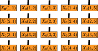
Figure 3: The 0-th representation of a 4 by 5 image as a TN diagram. We think of this TN not as an order-20 rank-1 tensor, but as just a collection of 20 vectors arranged on a grid.

For grayscale images, i.e. $C=1$, we set $Q_{0}=2$. In this case we can omit the dimension $C$. We must choose $\varphi:[0,1]\to\mathbb{R}^{Q_{0}}$. Possible choices include: (1) $\varphi(x)=\begin{bmatrix}\cos(\frac{\pi}{2}x)\\ \sin(\frac{\pi}{2}x)\end{bmatrix}$ [10, 2, 25, 12] encodes the value $x$ in a qubit. The components are nonnegative. It has $\ell_{2}$-norm equal to 1. (2) $\varphi(x)=\begin{bmatrix}x\\ 1-x\end{bmatrix}$ [17]. The components are nonnegative. It has $\ell_{1}$-norm equal to 1. (3) $\varphi(x)=\begin{bmatrix}\cos^{2}(\frac{\pi}{2}x)\\ \sin^{2}(\frac{\pi}{2}x)\end{bmatrix}$ [9]. The components are nonnegative. The authors say that the $\ell_{1}$-norm always being equal to 1 provides numerical stability.

In light of the duality of tensor networks and discrete undirected probabilistic graphical models [24, 9], the second and third choices can be viewed as encoding a number as a binary probability distribution. In our work, we use

$$\varphi(x)=\nu\begin{bmatrix}\cos^{2}(\frac{\pi}{2}x)\\ \sin^{2}(\frac{\pi}{2}x)\end{bmatrix},$$ (1)

where $\nu$ is some positive real number. The choice of $\nu$ is described in Section A.1.

When working with a colored dataset, we convert the images to YCbCr, normalize, and add a fourth channel of constant ones. In other words, we use

$$\phi\left(\begin{bmatrix}y&b&r\end{bmatrix}^{T}\right)=\begin{bmatrix}\frac{y-\mu_{y}}{\sigma_{y}}&\frac{b-\mu_{b}}{\sigma_{b}}&{r-\mu_{r}}{\sigma_{r}}&1\end{bmatrix}^{T},$$

where $\mu_{y},\mu_{b},\mu_{r},\sigma_{y},\sigma_{b},\sigma_{r}$ are means and standard deviations (over the training dataset) of the three channels Y, Cb, Cr, correspondingly.

3.2 Entangled plaquette states

Entangled plaquette states (EPS) is defined in [9] as a generalized TN, in which vectors arranged on a two-dimensional grid are contracted with tensors of parameters. Suppose $K$ is a small positive integer called the kernel size (having the same meaning as kernel size in Conv2d function). Suppose $Q_{\text{in}},Q_{\text{out}}$ are positive integers called the quantum dimension size of input and the quantum dimension size of output, respectively. Then an EPS is parametrized with an order-$(K^{2}+1)$ tensor $E\in\mathbb{R}^{Q_{\text{out}}\times Q_{\text{in}}\times\dots\times Q_{\text{in}}}$ with one dimension of size $Q_{\text{out}}$ and $K^{2}$ dimensions of size $Q_{\text{in}}$.

Suppose $H_{\text{in}}\geq K,W_{\text{in}}\geq K$ are integers denoting the height and width of an input $X_{\text{in}}$ consisting of $H_{\text{in}}W_{\text{in}}$ vectors $X_{\text{in}}(h,w)\in\mathbb{R}^{Q_{\text{in}}}$ arranged on a $H_{\text{in}}$ by $W_{\text{in}}$ grid. Then applying the EPS parametrized by $E$ to the input $X_{\text{in}}$ produces an output $X_{\text{out}}=\operatorname{eps}(E,X_{\text{in}})$ consisting of vectors $\operatorname{eps}(E,X_{\text{in}})(h,w)\in\mathbb{R}^{Q_{\text{out}}}$ arranged on a $H_{\text{out}}=H_{\text{in}}-K+1$ by $W_{\text{out}}=W_{\text{in}}-K+1$ grid defined as

$$X_{\text{out}}(h,w)=E\bar{\times}_{K^{2}+1}X_{\text{in}}(h+0,w+0)\bar{\times}_{K^{2}}X_{\text{in}}(h+0,w+1)\dots\bar{\times}_{2}X_{\text{in}}(h+K-1,w+K-1).$$ (2)

Figure 4 visualizes this formula and shows that an EPS applied to an input is a generalized TN. Using matricization $\operatorname{mat}(E)\in\mathbb{R}^{Q_{\text{out}}\times Q_{\text{in}}^{K^{2}}}$, this formula can be rewritten as

$$X_{\text{out}}(h,w)=\operatorname{mat}(E)\cdot\operatorname{vec}\left(\bigotimes_{h^{\prime}=0}^{K-1}\bigotimes_{w^{\prime}=0}^{K-1}X_{\text{in}}(h+h^{\prime},w+w^{\prime})\right).$$ (3)

Notice that application of an EPS to an input applies the same function to each $K\times K$ sliding window of the input. This provides two of the three properties described in Section 1.1: locality and parameter sharing.

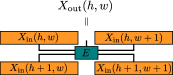
(a)

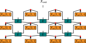
(b)

Figure 4: (a) One pixel of the output of an EPS with kernel size $K=2$ visualized as a TN diagram. The TN is equivalent to eqs. 2 and 3. (b) An EPS applied to an input is a generalized TN. Here $H_{\text{in}}=3,W_{\text{in}}=4,K=2$. Teal cores are identical. The output $X_{\text{out}}$ is a collection of 6 vectors. According to the terminology of [18], an EPS is a uniform TN.

EPS can be implemented as a backpropagatable function/layer and be used in neural networks or other gradient descent based models. The formulas for forward pass are given in eqs. 3 and 2. Next, we provide the backward pass formulas for derivatives. For $\frac{\partial\operatorname{eps}(E,X_{\text{in}})(h,w)}{\partial X_{\text{in}}(h^{\prime},w^{\prime})}\in\mathbb{R}^{Q_{\text{out}}\times Q_{\text{in}}}$, if $h^{\prime}\in\{h,\dots,h+K-1\}$ and $w^{\prime}\in\{w,\dots,w+K-1\}$, we have

$$\frac{\partial\operatorname{eps}(E,X_{\text{in}})(h,w)}{\partial X_{\text{in}}(h^{\prime},w^{\prime})}=E\underbrace{\operatorname{\bar{\times}}_{K^{2}+1}X_{\text{in}}(h+K-1,w+K-1)\cdots\operatorname{\bar{\times}}_{3}X_{\text{in}}(h,w+1)\operatorname{\bar{\times}}_{2}X_{\text{in}}(h,w)}_{\text{for each pair of indices }(h+\delta h,w+\delta w)\text{ except }(h+\delta h=h^{\prime},w+\delta w=w^{\prime})},$$

otherwise we have $\frac{\partial\operatorname{eps}(E,X_{\text{in}})(h,w)}{\partial X_{\text{in}}(h^{\prime},w^{\prime})}=0.$ For $\frac{\partial\operatorname{eps}(E,X_{\text{in}})(h,w)}{\partial E}\in\mathbb{R}^{Q_{\text{out}}\times Q_{\text{out}}\times Q_{\text{in}}\times\dots\times Q_{\text{in}}},$ denoting $I\in\mathbb{R}^{Q_{\text{out}}\times Q_{\text{out}}}$ to be the identity matrix, we have

$$\frac{\partial\operatorname{eps}(E,X_{\text{in}})(h,w)}{\partial E}=I\otimes\bigotimes_{\delta h=0}^{K-1}\bigotimes_{\delta w=0}^{K-1}X_{\text{in}}(h+\delta h,w+\delta w).$$

3.3 Description of the whole model

DCTN is a (functional) composition of the preprocessing function $\varphi$ described in Section 3.1, $N$ EPSes described in Section 3.2 parametrized by tensors $E_{1},\dots,E_{N}$, a linear layer parametrized by a matrix $A$ and a vector $b$, and the softmax function. The whole model is defined by

$$X_{0}(h,w)=\varphi(X(h,w))$$ (4)

$$X_{1}=\operatorname{eps}(E_{1},X_{0})$$ (5)

$$X_{2}=\operatorname{eps}(E_{2},X_{1})$$ (6)

$$\qquad\vdots$$

$$X_{N}=\operatorname{eps}(E_{N},X_{N-1})$$ (7)

$$\ln\hat{p}(y=\ell\mid X)=(A\cdot\operatorname{vec}(X_{N})+b)_{\ell}$$ (8)

$$p(y=\ell\mid X)=\operatorname{softmax}\left(\begin{bmatrix}\ln\hat{p}(y=1\mid X)\\ \ln\hat{p}(y=2\mid X)\\ \vdots\\ \ln\hat{p}(y=L\mid X)\end{bmatrix}\right)_{\ell}=\frac{\hat{p}(y=\ell\mid X)}{\sum_{\ell^{\prime}=1}^{L}\hat{p}(y=\ell^{\prime}\mid X)},$$ (9)

where $L$ is the number of labels. The original input image $X$ is represented as a tensor of shape $H_{0}\times W_{0}\times C$. For each $n$, the $n$-th intermediate representation $X_{n}$ consists of $H_{n}$ by $W_{n}$ vectors of size $Q_{n}$, and it holds that $H_{n}=H_{n-1}-K_{n}+1$, $W_{n}=W_{n-1}-K_{n}+1$, where $K_{n}$ is the kernel size of the $n$-th EPS. In principle, the affine function parametrized by $A$ and $b$ can be replaced with another differentiable possibly parametrized function, for example another tensor network.

A composition of EPSes is a TN. A composition of EPSes applied to an input is a generalized TN. See visualization in Figure 5.

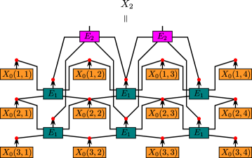
(a)

(b)

Figure 5: A composition of EPSes $E_{1},E_{2}$ with $K_{1}=K_{2}=2$. (a) A composition of EPSes applied to an input is a generalized TN. Here $H_{0}=3,W_{0}=4$. (b) A composition of EPSes is a TN, denoted $\operatorname{TN}(E_{1},\dots,E_{N})$. Here, $\operatorname{TN}(E_{1},E_{2})\in\mathbb{R}^{Q_{2}\times Q_{0}\times Q_{0}\times\dots\times Q_{0}}$ is an order-17 tensor. If you contract this TN with with a sliding window of an input (with some pixels copied), you’ll get one pixel of output.

3.4 Optimization

We initialize parameters $E_{1},\dots,E_{N}$ and $A,b$ of DCTN randomly. (Section A.1 contains details.) Let $\lambda\geq 0$ be the regularization coefficient. To train DCTN, at each iteration we sample $M$ images $X^{(1)},\dots,X^{(M)}$ and their labels $y^{(1)},\dots,y^{(M)}$ from the training dataset and use Adam optimizer [14] with either the objective

$$\underset{E_{1},\dots,E_{N},A,b}{\text{minimize}}\ \lambda\left(\left\lVert\operatorname{TN}(E_{1},\dots,E_{N})\right\rVert_{\text{fro}}^{2}+\left\lVert A\right\rVert_{\text{fro}}^{2}\right)+\frac{1}{M}\sum_{m=1}^{M}-\ln p\left(y^{(m)}\mid X^{(m)}\right),$$ (10)

where $\operatorname{TN}(E_{1},\dots,E_{N})$ is defined in Figure 5, or the objective

$$\underset{E_{1},\dots,E_{N},A,b}{\text{minimize}}\ \lambda\left(\left\lVert E_{1}\right\rVert_{\text{fro}}^{2}+\dots+\left\lVert E_{N}\right\rVert_{\text{fro}}^{2}+\left\lVert A\right\rVert_{\text{fro}}^{2}\right)+\frac{1}{M}\sum_{m=1}^{M}-\ln p\left(y^{(m)}\mid X^{(m)}\right).$$ (11)

We calculate the objective’s gradient with respect to the model’s parameters using backpropagation via Pytorch [22] autograd. We train the model in iterations, periodically evaluating it on the validation dataset, and take the model with the best validation accuracy as the final output of the training process.

4 Experiments

4.1 MNIST

We tested DCTN with one EPS, $\nu=0.5$ in eq. 1, $K_{1}=4,Q_{1}=4$, $\text{lr}=3\cdot 10^{-3}$, $\lambda=0$ in eq. 10, batch size 128 on MNIST dataset with 50000/10000/10000 training/validation/test split. We got 98.75% test accuracy. MNIST is considered relatively easy and doesn’t represent modern computer vision tasks [27].

4.2 FashionMNIST

FashionMNIST [28] is a dataset fully compatible with MNIST: it contains 70000 grayscale $28\times 28$ images. Each image belongs to one of 10 classes of clothes. We split 70000 images into 50000/10000/10000 training/validation/test split and experimented with models with one, two, and three EPSes. The more EPSes we used, the more overfitting DCTN experienced and the worse validation accuracy got, so we didn’t experiment with more than three EPSes. For one, two, and three EPSes, we chose hyperparameters by a combination of gridsearch and manual choosing and presented the best result (chosen by validation accuracy before being evaluated on the test dataset) in Table 1. In Appendix A, we describe more experiments and discuss how various hyperparameters affect optimization and generalization of DCTN.

Table 1: Comparison of our best models (top 3 rows) with 1, 2, and 3 EPSes, respectively, with the best (by a combination of accuracy and parameter count) existing models on FashionMNIST dataset. DCTN with one EPS wins against existing models with similar parameter count. Adding more EPSes makes test accuracy worse due to overfitting. All 3 of our models eventually reach nearly 100% accuracy if not stopped early. We trained all DCTNs with batch size 128.

Model	Accuracy	Parameter count
One EPS $K_{1}{=}4$, $Q_{1}{=}4$, $\nu{=}0.5$, $E_{1}{\sim}\mathcal{N}(\mu{=}0,\sigma{=}0.25)$, $A,b{\sim}U[-(H_{1}W_{1}Q_{1})^{-0.5},-(H_{1}W_{1}Q_{1})^{0.5}]$, $\text{lr}{=}3\cdot 10^{-3}$, $\lambda{=}0$, eq. 10	89.38%	$2.9\cdot 10^{5}$
Two EPSes, $K_{1}{=}4,Q_{1}{=}4,K_{2}{=}3,Q_{2}{=}6$, $\nu{\approx}1.46$, EPSes initialized from $\mathcal{N}(\mu{=}0,\sigma{=}Q_{\text{in}}^{-0.5K^{2}})$, $A{\sim}\mathcal{N}(\mu{=}0,\sigma{=}0.25(H_{2}W_{2}Q_{2})^{-0.5})$, $b{\sim}U[-(H_{2}W_{2}Q_{2})^{-0.5},(H_{2}W_{2}Q_{2})^{-0.5}]$, $\text{lr}{=}1.11\cdot 10^{-4}$, $\lambda{=}10^{-2}$, eq. 11	87.65%	$1.8\cdot 10^{6}$
Three EPSes, $K_{1}{=}4,Q_{1}{=}4,K_{2}{=}3,Q_{2}{=}12,K_{2}{=}2,Q_{2}{=}24$, $\nu{\approx}1.46$, EUSIR initialization of EPSes (see Section A.1), $A{\sim}\mathcal{N}(\mu{=}0,\sigma{=}0.25(H_{2}W_{2}Q_{2})^{-0.5})$, $b{\sim}U[-(H_{3}W_{3}Q_{3})^{-0.5},(H_{3}W_{3}Q_{3})^{-0.5}]$, $\text{lr}{=}10^{-7}$, $\lambda{=}10^{-1}$, eq. 10	75.94%	$4\cdot 10^{6}$
GoogleNet + Linear SVC	93.7%	$6.8\cdot 10^{6}$
VGG16	93.5%	$2.6\cdot 10^{7}$
CNN: 5x5 conv ->5x5 conv ->linear ->linear	91.6%	$3.3\cdot 10^{6}$
AlexNet + Linear SVC	89.9%	$6.2\cdot 10^{7}$
Matrix tensor train in snake pattern (Glasser 2019)	89.2%	?
Multilayer perceptron	88.33%	$2.3\cdot 10^{5}$

4.3 CIFAR10

CIFAR10 [15] is a colored dataset of 32 by 32 images in 10 classes. We used 45000/5000/10000 train/validation/test split. We evaluated DCTN on the colored version using YCbCr color scheme and on grayscale version which mimics MNIST and FashionMNIST. The results are in Table 2. DCTN overfits and performs poorly – barely better than a linear classifier. Our hypotheses for why DCTN performs poorly on CIFAR10 in contrast to MNIST and FashionMNIST are: (a) CIFAR10 images have much less zero values; (b) classifying CIFAR10 is a much more difficult problem; (c) making CIFAR10 grayscale loses too much useful information, while non-grayscale version has too many features, which leads to overfitting. In the future work, we are going to check these hypotheses with intensive numerical experiments.

Table 2: DCTN results on CIFAR10. For each number of color channels, for each number of EPSes, we chose the kernel sizes $K_{n}$, the quantum dimension sizes $Q_{n}$, and the learning rate using grid search (excluding models the training of which didn’t fit in 8 Gb of videocard’s RAM) and showed the best model in the table. All of these models can reach almost 100% training accuracy if not stopped early. Two bottom rows show the accuracy of a linear classifier and of one of the state of the art CNNs for comparison.

Channels	Model	Accuracy
Grayscale	One EPS, $K_{1}{=}4,Q_{1}{=}4$	49.5%
Grayscale	Two EPSes, $K_{1}{=}4,Q_{1}{=}4,K_{2}{=}3,Q_{2}{=}6$	54.8%
YCbCr	One EPS, $K_{1}{=}2,Q_{1}{=}24$	51%
YCbCr	Two EPSes, $K_{1}{=}2,Q_{1}{=}23,K_{2}{=}2,Q_{2}{=}24$	38.6%
RGB	Linear classifier	41.73%
RGB	EfficientNet-B7 [26]	98.9%

5 Conclusion

We showed that a tensor regression model can have locality, parameter sharing, and depth, just like a neural network. To check if such models are promising, we showed how to implement EPS as a backpropagatable function/layer and built a novel tensor regression model called DCTN consisting of a composition of EPSes. In principle, DCTN can be used for tasks for which deep CNNs are used.

We tested it for image classification on MNIST, FashionMNIST, and CIFAR10 datasets. We found that shallow DCTN with one EPS performs well on MNIST and FashionMNIST while having a small parameter. Unfortunately, adding more EPSes increased overfitting and thus made accuracy worse. Moreover, DCTN performed very badly on CIFAR10 regardless of depth. This suggests we can’t straightforwardly copy characteristics of NNs to make tensor regression work better. We think that overfitting is a large problem for tensor regression. In Appendix A, we have discussed how hyperparameters, such as initialization, input preprocessing, and learning rate affect optimization and overfitting. It seems that these hyperparameters have a large effect, but our understanding of this is limited. For example, we got our best model by scaling down the multiplier $\nu$ used in the input preprocessing function eq. 1. We think it’s important to study the effects of hyperparameters further and understand why some of them help fight overfitting.

Our code is free software and can be accessed at https://github.com/philip-bl/dctn.

Appendix A How hyperparameters affect optimization and generalization

In this section, we present some of our thoughts and findings about how the hyperparameters affect DCTN’s optimization and overfitting. Hopefully, they may prove useful for other tensor regression models as well. All empirical findings presented here were obtained on FashionMNIST dataset. They might not replicate on other datasets or with radically different values of hyperparameters.

A.1 Initialization of the model and scaling of the input

Consider a DCTN with $N$ EPSes and kernel sizes $K_{1},\dots,K_{N}$. Let $c>0$ be a positive real number. Then

$$A\cdot\operatorname{vec}\left(\operatorname{eps}(E_{N},\dots\operatorname{eps}(E_{1},cX_{0})\dots)\right)=c^{K_{1}^{2}\dots K_{N}^{2}}A\cdot\operatorname{vec}\left(\operatorname{eps}(E_{N},\dots\operatorname{eps}(E_{1},X_{0})\dots)\right)$$ (12)

and

$$A\cdot\operatorname{vec}\left(\operatorname{eps}(E_{N},\dots\operatorname{eps}(cE_{1},X_{0})\dots)\right)=c^{K_{2}^{2}\dots K_{N}^{2}}A\cdot\operatorname{vec}\left(\operatorname{eps}(E_{N},\dots\operatorname{eps}(E_{1},X_{0})\dots)\right).$$ (13)

Since $K_{1}^{2}K_{2}^{2}\dots K_{N}^{2}$ can get very large (e.g. 576 for $K_{1}=4,K_{2}=3,K_{3}=2$), it follows that if the constant $\nu$ in the input preprocessing function

$$\varphi(x)=\nu\begin{bmatrix}\cos^{2}(\frac{\pi}{2}x)\\ \sin^{2}(\frac{\pi}{2}x)\end{bmatrix}$$ (1)

is chosen slightly larger than optimal, eq. 12 might easily get infinities in floating point arithmetic, and if it’s chosen slightly smaller than optimal, eq. 12 might easily become all zeros, and the model’s output will stop depending on anything except the bias $b$.

The same is true in a slightly lesser degree for scaling of initial values of $E_{1},\dots,E_{N}$, especially for the earlier EPSes, as shown in eq. 13. Also, if for a chosen $\nu$ and chosen initialization of the EPSes, the values in

$$A\cdot\operatorname{vec}\left(\operatorname{eps}(E_{N},\dots\operatorname{eps}(E_{2},\operatorname{eps}(E_{1},X_{0}))\dots)\right)$$

have large standard deviation, then the values in the output of the whole model

$$A\cdot\operatorname{vec}\left(\operatorname{eps}(E_{N},\dots\operatorname{eps}(E_{2},\operatorname{eps}(E_{1},X_{0}))\dots)\right)+b$$

will have large standard deviation as well, which might lead to initial negative log likelihood being high. [13] recommends initializing neural networks for classification in such a way that initially the loss has the best possible value given that your model is allowed to know the proportion of labels in the datasets, but hasn’t been allowed to train yet. For example, if you have 10 possible labels with equal number of samples, a perfectly calibrated model that is ignorant about the images should have negative log likelihood equal to $\ln 10\approx 2.3$. We think that if the model starts with negative log likelihood much higher than this value, problems with the optimization process might occur.

One way we tried to overcome this difficulty was by adapting He initialization [11] for EPSes:

$$E\sim\mathcal{N}(\mu=0,\sigma=Q_{\text{in}}^{-0.5K^{2}}).$$ (14)

The rationale for this initialization is that if the components of $E\in\mathbb{R}^{Q_{\text{out}}\times Q_{\text{in}}\times\dots\times Q_{\text{in}}}$ are distributed i.i.d. with zero mean and variance $\alpha^{2}$, and if the components of $\omega\in\mathbb{R}^{Q_{\text{in}}\times\dots\times Q_{\text{in}}}$ are distributed i.i.d. with mean $\mu$ and variance $\sigma^{2}$, then, applying the EPS $E$ similar to eq. 3, we have

$$\mathbb{E}\left[\operatorname{mat}(E)\cdot\operatorname{vec}(\omega)\right]=0,$$

$$\operatorname{Var}\left[\operatorname{mat}(E)\cdot\operatorname{vec}(\omega)\right]=Q_{\text{in}}^{K^{2}}\alpha^{2}(\sigma^{2}+\mu^{2})I.$$

Note that the input $\omega$ having i.i.d. coordinates is not necessarily true in the real scenario, but still, we might try to initialize the EPSes using He initialization eq. 14. In this case, we choose such value for $\nu$ as to have the components of the vector

$$\operatorname{vec}\left(\bigotimes_{\delta h=0}^{K_{1}-1}\bigotimes_{\delta w=0}^{K_{1}-1}X_{0}(h+\delta h,w+\delta w)\right),$$

which appears in eq. 3, have empirical mean $\mu$ and empirical standard deviation $\sigma$ (over the whole training dataset) satisfy $\mu^{2}+\sigma^{2}=1$. For example, on FashionMNIST with our choice of $\varphi$, the value $\nu\approx 1.46$ satisfies this criterion, and that’s the value we use in 2 out of 3 experiments in Table 1.

However, empirically we’ve seen that with He initialization of a DCTN with 2 EPSes, the empirical standard deviation (over the whole training dataset) of the second intermediate representation $\operatorname{std}(X_{2})$ sometimes (depending on the random seed) is magnitudes larger or smaller than $1$. If it’s large, this leads to initial negative log likelihood loss being high, which we think might be bad for optimization. That’s why we devised another initialization scheme: while choosing $\nu$ the same way described earlier, we first initialize components of each EPS $E_{n}$ from the standard normal distribution and then rescale the EPS by the number required to make empirical standard deviation (over the whole training dataset) of its output $X_{n}$ equal to 1. In other words, here’s what we do:

$$\text{Initialize }E_{1}\sim\mathcal{N}(0,1)$$

$$\text{Multiply }E_{1}\text{ by the number that will make }\operatorname{std}(\operatorname{eps}(E_{1},X_{0}))=1$$

$$\text{Initialize }E_{2}\sim\mathcal{N}(0,1)$$

$$\text{Multiply }E_{2}\text{ by the number that will make }\operatorname{std}(\operatorname{eps}(E_{2},\operatorname{eps}(E_{1},X_{0})))=1$$

$$\vdots$$

$$\text{Initialize }E_{N}\sim\mathcal{N}(0,1)$$

$$\text{Multiply }E_{N}\text{ by the number that will make }\operatorname{std}(\operatorname{eps}(E_{N},\dots\operatorname{eps}(E_{1},X_{0})\dots))=1$$

We call this initialization scheme EUSIR initialization (empirical unit std of intermediate representations initialization). You can see a visualization of its effects in Figure 6.

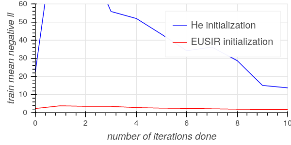
(a)

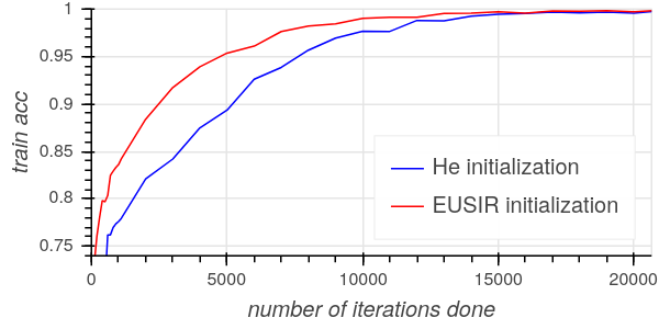
(b)

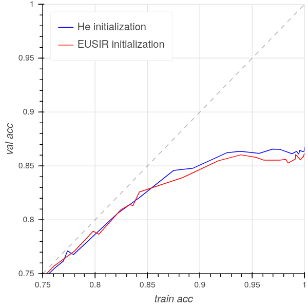
(c)

Figure 6: Comparison of He initialization and EUSIR initialization. (a) He initialization suffers from high initial loss. (b) EUSIR initialization trains faster. (c) Unfortunately, this didn’t lead to less overfitting. In all three plots, the model consists of 2 EPSes with $K_{1}{=}3,Q_{1}{=}4,K_{2}{=}3,Q_{2}{=}6,\text{lr}=4\cdot 10^{-5},\lambda=10^{-2}$, and the objective function eq. 10.

A.2 Other hyperparameters

• Figure 7 discusses how high learning rate leads to less overfitting.

• Figure 8 discusses how we accidentally got the best result with one EPS by setting a very small $\nu$.

• In our experiments, $\ell_{2}$ regularization coefficient $\lambda$ affected neither training speed nor validation accuracy. We don’t provide plots depicting this, because they would show nearly identical training trajectories for different values of $\lambda$ from $0$ to $10^{-2}$.

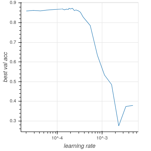
(a)

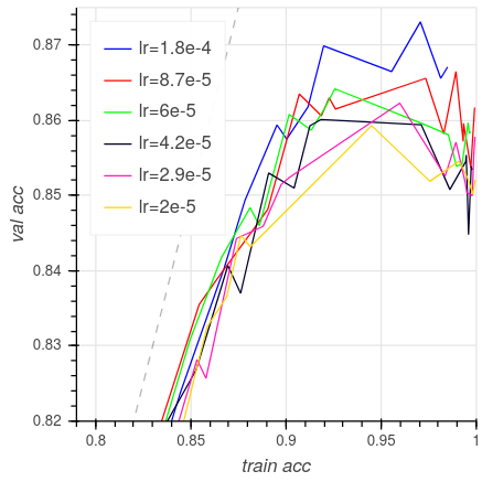
(b)

Figure 7: As can be seen in (a), too large learning rate causes training to not converge. However (b) shows that large but not too large learning rate slightly reduces overfitting (training trajectories with higher learning rate achieve higher validation accuracy). This is in line with folk understanding of how learning rate affects training in deep learning. The model had 2 EPSes with $K_{1}{=}4,Q_{1}{=}4,K_{2}{=}3,Q_{2}{=}=6,\lambda=10^{-2}$, used the objective function eq. 10 and EUSIR initialization.

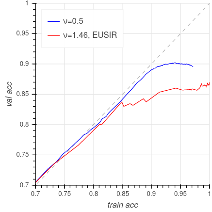
(a)

(b)

Figure 8: The plot (a) shows how a model we made by accidentally altering hyperparameters achieves better generalization. However, it trained 960 times slower, as can be seen in (b). Both models have one EPS with $K_{1}{=}4,Q_{1}{=}4,\text{lr}{=}3\cdot 10^{-3},\lambda=0$, $A,b\sim U[-0.02,0.02]$. The difference is in the choice of $\nu$ and in initialization of EPSes. The blue model is the model from the first row of Table 1. It has $\nu{=}0.5$ and its intermediate representations have standard deviations $\operatorname{std}(X_{1}){\approx}1.7\cdot 10^{-6}$, $\operatorname{std}(A\cdot\operatorname{vec}(X_{1})){\approx}1.1\cdot 10^{-6}$. The red model uses $\nu{\approx}1.46$, EUSIR initialization and thus has, $\operatorname{std}(X_{1}){=}1$. Notice that the standard deviation of the output of linear layer of the blue model, if we don’t add the bias $b$, is very small compared to the standard deviation of the bias $b$. We speculate that this is probably the reason of much better generalization. It important to understand why the blue model’s initialization and the choice of $\nu$ worked so well and figure out how to achieve it with more EPSes.

References

- Alammar [2018] Alammar. The illustrated transformer. https://jalammar.github.io/illustrated-transformer, 2018. Accessed: 2020-09-30.
- Bhatia et al. [2019] Amandeep Singh Bhatia, Mandeep Kaur Saggi, Ajay Kumar, and Sushma Jain. Matrix product state–based quantum classifier. Neural computation, 31(7):1499–1517, 2019.
- Biamonte and Bergholm [2017] Jacob Biamonte and Ville Bergholm. Tensor networks in a nutshell. arXiv preprint arXiv:1708.00006, 2017.
- Bridgeman and Chubb [2017] Jacob C Bridgeman and Christopher T Chubb. Hand-waving and interpretive dance: an introductory course on tensor networks. Journal of Physics A: Mathematical and Theoretical, 50(22):223001, 2017.
- Cichocki et al. [2017] A Cichocki, AH Phan, I Oseledets, Q Zhao, M Sugiyama, N Lee, and D Mandic. Tensor networks for dimensionality reduction and large-scale optimizations: Part 2 applications and future perspectives. Foundations and Trends in Machine Learning, 9(6):431–673, 2017.
- Cichocki et al. [2016] Andrzej Cichocki, Namgil Lee, Ivan V Oseledets, A-H Phan, Qibin Zhao, and D Mandic. Low-rank tensor networks for dimensionality reduction and large-scale optimization problems: Perspectives and challenges part 1. arXiv preprint arXiv:1609.00893, 2016.
- Cohen et al. [2016] Nadav Cohen, Or Sharir, and Amnon Shashua. On the expressive power of deep learning: A tensor analysis. In Conference on Learning Theory, pages 698–728, 2016.
- Ehrbar [2000] Hans G Ehrbar. Graph notation for arrays. ACM SIGAPL APL Quote Quad, 31(3):13–26, 2000.
- Glasser et al. [2020] I. Glasser, N. Pancotti, and J. I. Cirac. From probabilistic graphical models to generalized tensor networks for supervised learning. IEEE Access, 8:68169–68182, 2020.
- Grant et al. [2018] Edward Grant, Marcello Benedetti, Shuxiang Cao, Andrew Hallam, Joshua Lockhart, Vid Stojevic, Andrew G Green, and Simone Severini. Hierarchical quantum classifiers. npj Quantum Information, 4(1):1–8, 2018.
- He et al. [2015] Kaiming He, Xiangyu Zhang, Shaoqing Ren, and Jian Sun. Delving deep into rectifiers: Surpassing human-level performance on imagenet classification. In Proceedings of the IEEE international conference on computer vision, pages 1026–1034, 2015.
- Huggins et al. [2019] William Huggins, Piyush Patil, Bradley Mitchell, K Birgitta Whaley, and E Miles Stoudenmire. Towards quantum machine learning with tensor networks. Quantum Science and technology, 4(2):024001, 2019.
- Karpathy [2019] Karpathy. A recipe for training neural networks. https://karpathy.github.io/2019/04/25/recipe, 2019. Accessed: 2020-05-25.
- Kingma and Ba [2014] Diederik P Kingma and Jimmy Ba. Adam: A method for stochastic optimization. arXiv preprint arXiv:1412.6980, 2014.
- Krizhevsky et al. [2009] Alex Krizhevsky, Geoffrey Hinton, et al. Learning multiple layers of features from tiny images. 2009.
- Liu et al. [2019] Ding Liu, Shi-Ju Ran, Peter Wittek, Cheng Peng, Raul Blázquez García, Gang Su, and Maciej Lewenstein. Machine learning by unitary tensor network of hierarchical tree structure. New Journal of Physics, 21(7):073059, 2019.
- Miller [2019] Jacob Miller. Torchmps. https://github.com/jemisjoky/torchmps, 2019.
- Miller et al. [2020] Jacob Miller, Guillaume Rabusseau, and John Terilla. Tensor networks for probabilistic sequence modeling, 2020.
- Novikov et al. [2016] Alexander Novikov, Mikhail Trofimov, and Ivan Oseledets. Exponential machines. arXiv preprint arXiv:1605.03795, 2016.
- Orús [2014] Román Orús. A practical introduction to tensor networks: Matrix product states and projected entangled pair states. Annals of Physics, 349:117–158, 2014.
- PapersWithCode [2020] PapersWithCode. Browse the state-of-the-art in machine learning. https://paperswithcode.com/sota, 2020. Accessed: 2020-05-23.
- Paszke et al. [2019] Adam Paszke, Sam Gross, Francisco Massa, Adam Lerer, James Bradbury, Gregory Chanan, Trevor Killeen, Zeming Lin, Natalia Gimelshein, Luca Antiga, Alban Desmaison, Andreas Kopf, Edward Yang, Zachary DeVito, Martin Raison, Alykhan Tejani, Sasank Chilamkurthy, Benoit Steiner, Lu Fang, Junjie Bai, and Soumith Chintala. Pytorch: An imperative style, high-performance deep learning library. In H. Wallach, H. Larochelle, A. Beygelzimer, F. d'Alché-Buc, E. Fox, and R. Garnett, editors, Advances in Neural Information Processing Systems 32, pages 8024–8035. Curran Associates, Inc., 2019. URL http://papers.neurips.cc/paper/9015-pytorch-an-imperative-style-high-performance-deep-learning-library.pdf.
- Polu and Sutskever [2020] Stanislas Polu and Ilya Sutskever. Generative language modeling for automated theorem proving, 2020.
- Robeva and Seigal [2019] Elina Robeva and Anna Seigal. Duality of graphical models and tensor networks. Information and Inference: A Journal of the IMA, 8(2):273–288, 2019.
- Stoudenmire and Schwab [2016] E. Miles Stoudenmire and David J. Schwab. Supervised learning with quantum-inspired tensor networks, 2016.
- Tan and Le [2020] Mingxing Tan and Quoc V. Le. Efficientnet: Rethinking model scaling for convolutional neural networks, 2020.
- Xiao et al. [2017a] Han Xiao, Kashif Rasul, and Roland Vollgraf. Fashionmnist readme. https://github.com/zalandoresearch/fashion-mnist/blob/master/README.md, 2017a. Accessed: 2020-05-24.
- Xiao et al. [2017b] Han Xiao, Kashif Rasul, and Roland Vollgraf. Fashion-mnist: a novel image dataset for benchmarking machine learning algorithms. arXiv preprint arXiv:1708.07747, 2017b.