A high-resolution cosmological simulation of a strong gravitational lens

Abstract

We present a cosmological hydrodynamical simulation of a $10^{13}$ M_⊙ galaxy group and its environment (out to 10 times the virial radius) carried out using the Eagle model of galaxy formation. Exploiting a novel technique to increase the resolution of the dark matter calculation independently of that of the gas, the simulation resolves dark matter haloes and subhaloes of mass $5\times 10^{6}$ M_⊙. It is therefore useful for studying the abundance and properties of the haloes and subhaloes targeted in strong lensing tests of the cold dark matter model. We estimate the halo and subhalo mass functions and discuss how they are affected both by the inclusion of baryons in the simulation and by the environment. We find that the halo and subhalo mass functions have lower amplitude in the hydrodynamical simulation than in its dark matter only counterpart. This reflects the reduced growth of haloes in the hydrodynamical simulation due to the early loss of gas by reionisation and galactic winds and, additionally, in the case of subhaloes, disruption by enhanced tidal effects within the host halo due to the presence of a massive central galaxy. The distribution of haloes is highly anisotropic reflecting the filamentary character of mass accretion onto the cluster. As a result, there is significant variation in the number of structures with viewing direction. The median number of structures near the centre of the halo, when viewed in projection, is reduced by a factor of two when baryons are included.

1 Introduction

Compelling evidence for the existence of non-baryonic dark matter particles is provided by the temperature structure of the cosmic microwave background radiation (Planck Collaboration et al., 2016) and supported by observations of gravitational lensing (see Massey et al., 2010, for a review). Measurements of the cosmic large-scale structure set constraints on the properties of the particles. Thus, the observed large-scale distribution of galaxies rules out hot dark matter, that is, particles with large primordial thermal velocities, as the main form of dark matter (Frenk et al., 1983; White et al., 1983, 1984). On the other hand, the data are in excellent agreement with the cold dark matter (CDM) model, in which the particles have negligible primordial thermal velocities (Davis et al., 1985; Springel et al., 2005; Rodríguez-Torres et al., 2016). Warm dark matter (WDM) models represent the current upper bound on the primordial velocity distribution of the dark matter particle. Testing these models serves to constrain the properties of dark matter in the early Universe and also to guide searches for the fundamental particle nature of dark matter.

The main distinguishing difference between the CDM and WDM models is the predicted abundance of structures on the scale of dwarf galaxies and below (Colín et al., 2000; Bode et al., 2001; Lovell et al., 2012; Schneider et al., 2012a; Kennedy et al., 2014). Current WDM models of interest, for example a 7 keV sterile neutrino, predict an exponential reduction in the abundance of structure below a mass of approximately $10^{8}$ M_⊙ (Lovell et al., 2012; Schneider et al., 2013; Hellwing et al., 2016; Bose et al., 2017; Lovell et al., 2017); by contrast, in the CDM model the halo mass function continues to increases towards low masses (Diemand et al., 2007; Springel et al., 2008). Precise measurements of the abundance of such low mass haloes would constrain WDM models and, if they were shown to be absent, would conclusively rule out the CDM model.

Galaxies cannot form in halos of mass $\lesssim 10^{8}$M_⊙ (Sawala et al., 2013; Sawala et al., 2016; Benitez-Llambay & Frenk, 2020) so these can only be detected through gravitational lensing effects, particularly the distortions they cause to the images of strong lensing arcs produced by much more massive lenses such as groups and clusters of galaxies (Koopmans, 2005). This method has already been used successfully to detect a $1.9\pm 0.1\times 10^{8}$ M_⊙ dark satellite and the detection sensitivity is expected to reach $\sim 2\times 10^{7}$ M_⊙ (Vegetti et al., 2012). Li et al. (2017) estimate that analysis of about 100 strong lensing systems could conclusively distinguish CDM from the 7 keV sterile neutrino WDM models, while samples of quadruply imaged quasars have already been used to infer that the halo mass function continues down to masses $\lesssim 10^{7.8}$ M_⊙ (Gilman et al., 2020).

Li et al. (2017) and Despali et al. (2018) based their predictions of the subhalo and field halo contributions to the lensing signal on dark-matter-only (DMO) simulations. It is now well established that the inclusion of baryons in the simulations has important effects on the population of small-mass subhalos orbiting in Milky Way mass haloes (D’Onghia et al., 2010; Sawala et al., 2017; Garrison-Kimmel et al., 2017; Richings et al., 2020), leading to a reduction in the abundance of subhaloes near the centre of the host of at least 50%. The size of these effects in general depends on the size and shape of the galaxy at the centre. Haloes that produce visible lens arcs are typically ten times more massive than the Milky Way halo (Bolton et al., 2008) and the galaxies that form at their centres are different in size and morphology to the Milky Way.

Simulating $10^{13}$ M_⊙ haloes with a small enough particle mass to resolve the population of $10^{7}$ M_⊙ subhaloes necessary for strong lensing tests, whilst also including the effects of baryons at sufficient resolution, is computationally prohibitive with conventional techniques. Here we describe and implement a new technique for setting up the initial conditions of a cosmological simulation, so that dark matter particles outnumber gas particles by 7:1. This approach allows us to resolve $10^{7}$ M_⊙ substructures within a $10^{13}$ M_⊙ halo, whilst following the gas dynamics at the full resolution of the high-resolution Eagle simulation, ${\sim}10^{5}$M_⊙ (Schaye et al., 2015). In the simulation described here, the masses of dark matter and gas particles are approximately equal. This approach has the added benefit of avoiding the spurious growth in the sizes of galaxies described by Ludlow et al. (2019), caused by gravitational two-body scattering of unequal-mass particles imparting velocity kicks to the lighter particles.

This paper is arranged as follows: in §2 we describe the creation and testing of the initial conditions of our simulation, as well as some key diagnostics of the completed simulation. In §3 we examine the effect of both baryons and environment on the abundance and properties of field halos. This section also includes a discussion of the definition of the mass of a halo. In §4 we study the abundance and concentration of subhalos in the central halo of the simulation. We also consider the variation in the observed abundance of structure due to projection effects. We conclude in §5.

2 Simulations

The simulation was performed using the Eagle Reference model (Schaye et al., 2015; Crain et al., 2015) with one exception: in addition to the fiducial star formation rate calculation, any gas particle reaching a density $n_{\mathrm{H}}>10^{4}\,\rm{cm}^{-3}$ was directly converted into a star particle..

2.1 Candidate selection

It is important that the halo and associated central galaxy selected for resimulation be representative of those that produce observed lenses. Despali & Vegetti (2017) identified a sample of halos in the Eagle 100 Mpc simulation (Schaye et al., 2015) which have similar properties to lenses detected in the SLACS Survey (Bolton et al., 2006). This was designed to detect bright, early-type lens galaxies, the most suitable for detailed lensing and photometric studies, at $z\sim 0.2$.

The following criteria were used:

• The halo is at a redshift of approximately $z=0.2$.

• The halo must be relaxed (according the criteria of Neto et al. 2007).

• The halo has a virial mass between $10^{12}$–$10^{14.5}$ M_⊙. (Less massive halos will not produce visible Einstein rings.)

• The halo has a velocity dispersion of between 160–400 km/s. inside the half-mass radius.

• The central galaxy is an Elliptical. Specifically, at least 25% of all star particles inside 20 kpc must be counter rotating, where direction of rotation is given by the total angular momentum of all the star particles in this region.

From the sample of halos we select one object for resimulation. In the Eagle 100 Mpc volume run with the Reference subgrid model, the halo has a FOF ID of 129, a mass of $M_{200}=10^{13.1}$ M_⊙, and is located at at [89.742, 42.189, 94.507] Mpc.

2.2 Construction of initial conditions

We use a zoom simulation (Frenk et al., 1996) to study the selected halo. This allows us to resolve the low-mass substructures relevant for tests of the CDM model whilst minimising the computational burden. We find all particles which are less than 5.5 Mpc from the potential minimum of the halo at redshift $z=0.2$. We then identify these particles in the Eagle simulation initial conditions and trace them back to their comoving coordinates at the Big Bang using the Zel’dovich approximation (Zel’dovich, 1970). This defines the region of space known as the Lagrangian region, which is the patch of the universe from which our target halo will form.

To perform a zoom simulation, the Lagrangian region is populated with particles which have smaller masses than the particles of the parent simulation. The rest of the volume is populated with more massive particles, present only to reproduce the correct large-scale tidal forces without significantly increasing the overall computational cost. The particles which populate the Lagrangian region must be arranged such that (i) the whole region has the mean density of the universe, (ii)  the configuration of particles is very close to being gravitationally stable. Any instabilities in the initial conditions which are not to due physical effects will lead to the rapid growth of artificial structure.

For DMO zoom simulations, the Lagrangian region can simply be populated with a uniformly-spaced grid. A common approach for simulations using the smooth particle hydrodynamics (SPH) technique is to take the uniform grid of DMO particles and split each particle into a gas particle and a dark matter particle. The total mass of each pair is kept the same as the DMO particle, and the particles are placed such that their centre of mass is the same as the position of the DMO particle. In this setup there is one dark matter particle per gas particle, and the ratio of the particle masses is determined by the cosmological parameters of the simulation, i.e. $m_{\mathrm{DM}}/m_{\mathrm{gas}}\equiv\Omega_{\mathrm{DM}}/\Omega_{\mathrm{b}}$. In the Planck 2015 cosmology, this means that each dark matter particle is 5.36 times heavier than a gas particle.

Our approach differs from the method outlined above in that the initial conditions are created with 7 dark matter particles per gas particle. This means that the ratio of the particle masses is given by $m_{\mathrm{DM}}/m_{\mathrm{gas}}\equiv\Omega_{\mathrm{DM}}/7\Omega_{\mathrm{b}}\sim 0.77$. To ensure uniform matter density, and to avoid gravitational instabilities (especially at the boundary of the Lagrangian region), we tesselate the Lagrangian region with a template as shown in Fig. 1.

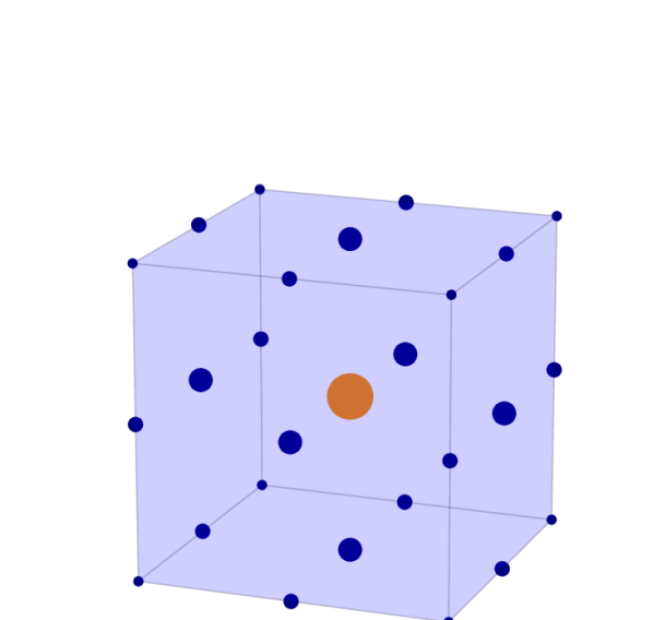
Figure 1: Template set of particles used to populate the Lagrangian region of the initial conditions. Dark matter particles are blue, and the gas particle is orange. The area of each particle in the diagram is directly proportional to its mass.

Each template contains one gas particle, which sits at the centre of the cell. The template also contains 26 “fractional” dark matter particles, positioned symmetrically on the faces, edges and vertices of the cell. When two templates are placed next to each other, some particles from each template will occupy the same position as particles from the template next door. These coincident fractional particles are combined into one whole particle, with a mass equal to the combined mass of the original particles. In the interior of the Lagrangian region, each face particle will overlap with one other face particle, each edge particle will overlap with three other edge particles, and each vertex particle will overlap with seven other vertex particles. Therefore in order for the masses of all the dark matter particles in the interior of the Lagrangian region to have the same target mass, the mass of each face particle in the template is one half of the target mass. Similarly, the edge and vertex particles in the template have masses of one quarter and one eighth of the target particle mass respectively.

The total number of dark matter particles per template in the interior of the Lagrangian region is thus given by $6/2+12/4+8/8=7$. Once the Lagrangian region has been populated with copies of the template, almost all dark matter particles will have the same mass, except for dark matter particles at the boundary, which will have some fraction of the target dark matter mass. These fractional masses at the edge of the Lagrangian region are necessary to ensure uniform density and gravitational stability. As the gas particle is placed at the centre of the template all the gas particle masses in the Lagrangian region will be the same.

Outside of the high resolution region, the tidal particles were placed using the method adopted for the Aquarius simulations (Springel et al., 2008). Because the tiling method for the high resolution is new, as a precaution, we did an additional test on the particle load. We created a full set of initial conditions with no cosmological perturbations and ran a simulation from our intended start redshift 127 to redshift zero.

No structures formed within the high resolution region. Not unexpectedly, some clustering occurred at the interface between the high resolution region and the lightest mass tidal particles. This structure formation, which is numerical in origin, was limited to a thin surface only. The velocities remained small except close to this surface. This indicates that the high resolution region in the particle load is at precisely the mean density of the universe as intended. The dark matter particles in this boundary region have masses that differ from those in the interior of the Lagrangian region. We excluded these particles, as well as all other tidal particles from the analysis.

The cosmological parameters used for the simulation are taken from the Planck 2013 results (Planck Collaboration et al., 2014) and are listed in Table 1. The table also lists the gravitational softening length used in the high-resolution region of our simulation and the masses of the dark matter and gas particles in the initial conditions. The initial conditions contain about 198 million gas particles and 1.393 billion dark matter particles in the high resolution region. In addition there are about 76 million more massive ‘tidal’ dark matter particles which surround the high resolution region and fill the entire computational volume.

Cosmological parameter	Value
$\Omega_{m}$	0.307
$\Omega_{\Lambda}$	0.693
$\Omega_{b}$	0.04825
$h\equiv H_{0}$/(100 km s-1 Mpc-1)	0.6777
$\sigma_{8}$	0.8288
$n_{s}$	0.9611
$Y$	0.248
$l_{\mathrm{box}}$ [cMpc]	100
$\epsilon_{0}$ [kpc]	0.05
$m_{\mathrm{DM}}$ [$10^{4}$ M⊙]	8.27
$m_{\mathrm{gas}}$ [$10^{4}$ M⊙]	10.74

Table 1: Cosmological and numerical parameters used in the simulation. $\Omega_{m}$, $\Omega_{\Lambda}$ and $\Omega_{b}$ are the mean density of matter, dark energy and baryons in units of the critical density at redshift $z=0$; $H_{0}$ is the value of the Hubble parameter at redshift $z=0$; $\sigma_{8}$ is the standard deviation of the linear matter distribution smoothed with a top hat filter of radius 8 $h^{-1}$ cMpc; $n_{s}$ is the index of the power law which describes the power spectrum of primordial fluctuations; $Y$ is the primordial abundance of helium; $\l_{\mathrm{box}}$ is the comoving side length of the simulation box; $\epsilon_{0}$ is the softening length used in the force calculations for high-resolution dark matter and gas particles at redshift $z=0$. $m_{\mathrm{DM}}$ is the mass of a dark matter particle in the high-resolution region of the hydrodynamical version of the simulation. Edge effects in the construction of the initial conditions mean that a tiny fraction of the high-resolution dark matter particles (approximately 1.5%) have masses which are a fraction of this value.

2.3 Testing the initial conditions

Changing the number of dark matter particles per gas particle can potentially affect important observables in the final simulation. For example, gravitational two-body scattering between species of different masses influence observables like the size of small galaxies (Ludlow et al., 2019). To study the effects of increasing the dark matter resolution for a fixed gas mass, we ran a 25 Mpc cosmological volume with 376³ gas particles and the same initial phases as the L0025N0376 volume described in Schaye et al. (2015), but with seven times as many dark matter particles. We refer to the original run as the standard-resolution (SR) simulation, and our new volume as the DMx7 simulation. The mass of gas particles in these two simulation are the same, but our version has seven times as many dark matter particles, that is our simulation has the standard Eagle gas resolution, but a dark matter resolution similar to that of the Eagle high-resolution (HR) run (L0025N0752).

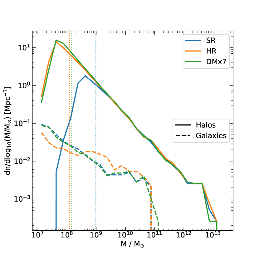
Figure 2: The mass function of halos (solid lines, $M=M_{200}$) and galaxies (dashed lines, $M=M_{\star}(<30\,\mathrm{kpc})$) in three realisations of the Eagle 25 Mpc simulation. The blue lines show the halo and galaxy mass functions at standard Eagle resolution. The orange lines show the effect of increasing the resolution of both gas and dark matter in the simulation, while the green lines show the effect of only increasing the resolution of dark matter whilst holding the gas resolution constant, as described in §2.2. Dotted lines show the mass of 100 DM particles in each simulation.

We checked several key properties, the first of which is the mass function of halos and galaxies. Here we take the mass of a galaxy to be the mass of all star particles within 30 kpc of the potential minimum of the host halo. These properties are shown in Fig. 2. The mass function of galaxies is almost unchanged between the versions of the simulation which have the same number of gas particles but different numbers of dark matter particles. The effect of increasing the resolution of gas particles has a much more significant impact on the abundance of both smaller and larger galaxies. The DMx7 simulation also does an excellent job of reproducing the halo mass function at masses below the resolution limit of the SR simulation. In general, if the difference between the blue and orange lines is bigger than the difference between either blue-green or orange-green, we conclude that the effect of increasing the gas resolution is more significant than the effect of changing the dark matter-gas mass ratio.

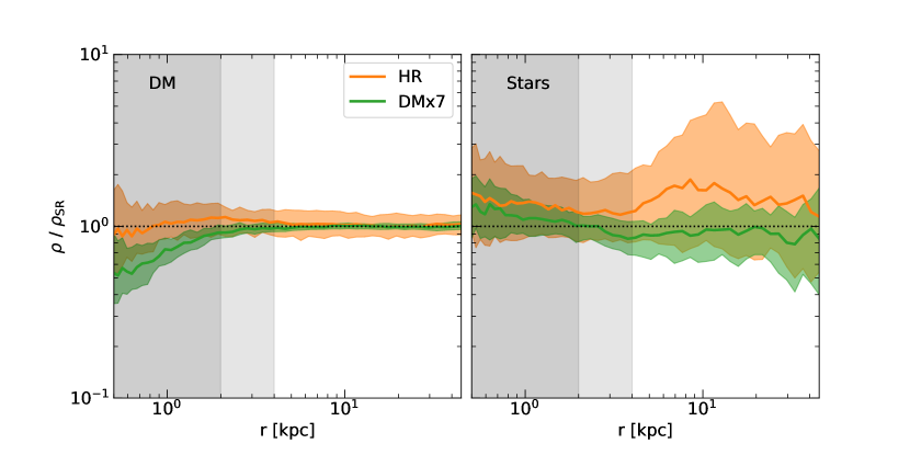
Figure 3: The ratio of the density of dark matter and stars in the HR (orange lines) and DMx7 (green lines) simulations to the density of dark matter and stars in the Eagle SR 25 Mpc simulation. The sample contains 100 halos bijectively matched between simulations. Solid lines show the median ratio as a function of radius for each species. Shaded regions indicate the interquartile range. The light grey shaded region shows the approximate value of the Power et al. 2003 radius for the SR simulation, whilst the dark grey region shows the corresponding radius for the HR and DMx7 simulations.

We also tested the effect of differing species resolution on the internal structure of halos. We matched halos between simulations by mass and position. Specifically, the masses of a potential matched pair must be within a factor of two, and the first halo must lie within the virial radius of the second halo and vice versa. This procedure produces a unique match for each of the 100 most massive halos in the SR simulation. Each halo in the SR simulation has a corresponding matched halo in the HR and DMx7 simulations. We calculated the density of dark matter and stars as a function of radius in each halo. For each species, we then calculate the ratio of density in the HR and DMx7 to the density in SR simulation. We performed this calculation for the 100 most massive halos in each simulation, which span a mass range of approximately $10^{11.5}$–$10^{13.5}$ M_⊙. The results are shown in Fig. 3.

Outside the Power et al. (2003) radius, all three versions of the simulations display excellent agreement in the measured dark matter density profiles. At distances of less than 5 kpc from the centre of the halo, the density of dark matter in the DMx7 simulation is significantly lower than in the simulations which have a standard gas to dark matter particle mass ratio. This result is not unexpected. Ludlow et al. (2019) have shown that the equipartition of energy between multiple species of different-mass particles causes the heavier species to sink artificially towards the centre of the halo. In the case of the SR simulation, the dark matter particles are around five times heavier than the star particles, which causes an artificial increase in the density of dark matter at the centre of the halo.

The second panel of Fig. 3 shows that beyond the Power et al. (2003) radius, where energy equipartition can affect the distribution of particles, the density of stars is generally well reproduced in the DMx7 simulation, albeit with considerable scatter. The same cannot be said for the HR simulation, where the effect of increasing gas resolution has a pronounced effect on the distribution of stars in galaxies. The key takeaway is that the uncertainties in the modelling of baryonic effects are significantly larger than variations introduced by altering the ratio of the mass of dark matter and gas particles.

2.4 The simulation

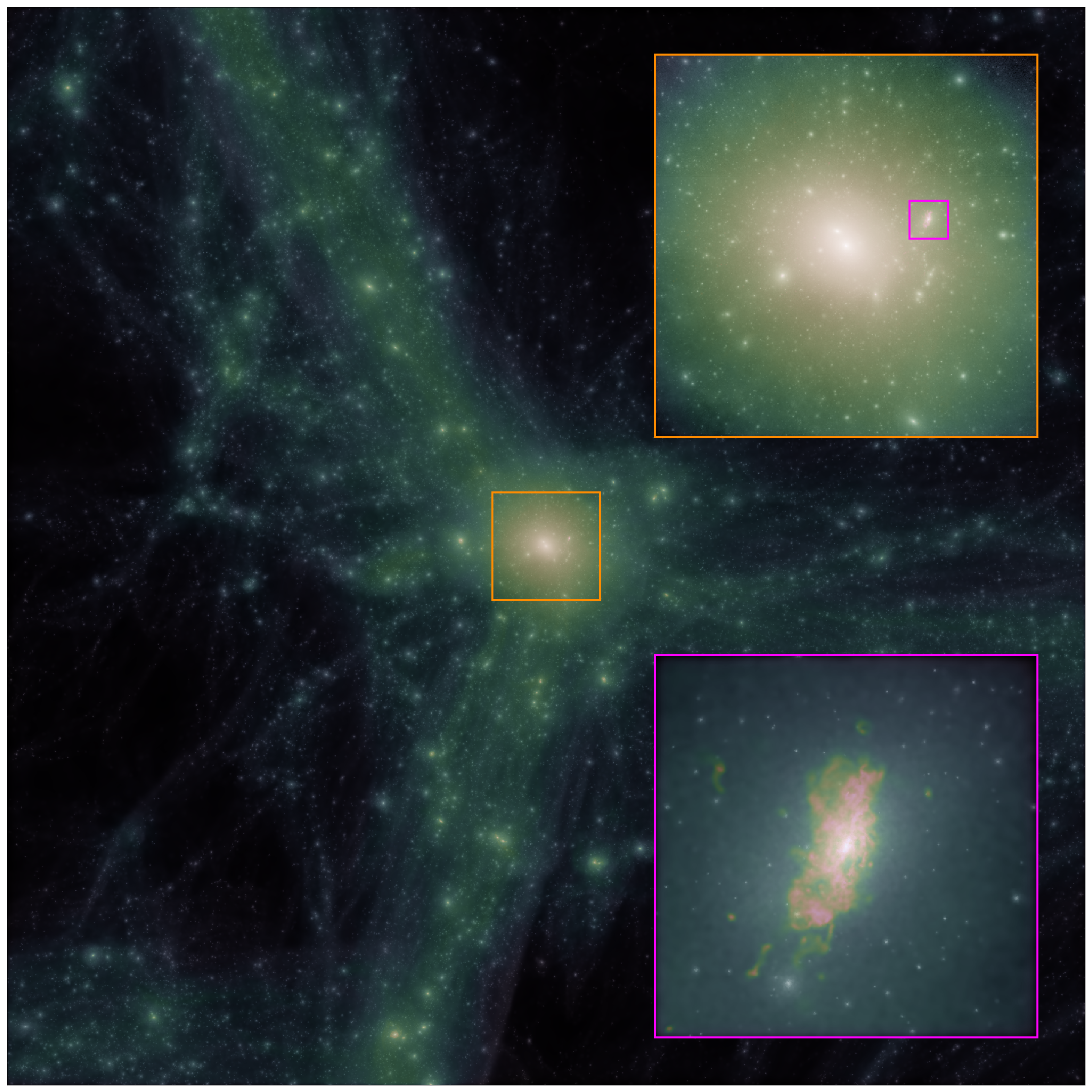
Figure 4: Projected density of matter in a cube of side length 10 Mpc, centred on the most massive halo in the high-resolution region of the simulation. The brightness of each pixel is proportional to the logarithm of the density of matter, and the hue encodes the density of gas. The orange inset shows a zoom into the largest halo, with a side length of 1 Mpc, and the pink inset shows a zoom into the subhalo with the greatest baryonic mass in the main halo, with a side length of 100 kpc. The main image contains approximately 500 million particles, whilst the image in the pink inset is based on approximately 1.8 million particles.

A visualisation of the high-resolution region of the simulation is shown in Fig. 4. The brightness of each pixel in the image is proportional to the logarithm of the projected density of matter, in a cube of side length 10 Mpc. The projected density of gas in the simulation is encoded in the hue of each pixel. Fig. 4 shows that the main halo in our simulation sits at the centre of three large filaments. The inset panels demonstrate the large dynamic range of the simulation, with the volume of the cube shown in the pink square being a millionth of the volume shown in the main figure. In addition to the excellent resolution of the central halo, our simulation also resolves the internal structure of the filaments of the cosmic web, including strands of filaments that are almost entirely devoid of baryonic matter.

The region simulated at high resolution is unusually large for a zoom simulation. The region is approximately spherical, with a radius of around 7 Mpc at redshift $z=0$. This is approximately 14 times the virial radius of the main halo. For comparison, the high-resolution region in the Hydrangea cluster simulations is 10 times the virial radius (Bahé et al., 2017) and is 4-5 times the virial radius (or around 1 Mpc in absolute terms) for the Auriga suite of galactic zoom simulations (Grand et al., 2016). The largest halo in the high-resolution region (to which we will hereafter refer as the main halo) has a mass of $M_{200}=10^{13.14}$ M_⊙ and a radius of $r_{200}=506$ kpc at redshift $z=0$. This halo contains 200 million particles (as identified using the standard friends-of-friends algorithm; Davis et al. 1985). Running this hydrodynamical version of this simulation required around 1.5 million core-hours, on 512 cores.

3 The halo population

In this section we examine the field halos in our simulation. In particular, we focus on the halo mass function in the mass range $10^{6.5}$–$10^{10.5}$ M_⊙, critical for studies of strong gravitational lensing by massive elliptical galaxies designed to test the $\Lambda$CDM model and to distinguish CDM from viable alternatives such as WDM in the form of 7 keV sterile neutrinos. We discuss the effects of baryons on the halo mass function, and compare the measured halo mass function to predictions of the widely used Sheth-Tormen model (Sheth & Tormen, 2002). We also study the relationship between halo properties and their environment, specifically the abundance of halos in different environments and the relationship between halo environment and internal halo structure.

3.1 The mass of a halo

There is no unique way to define the mass of halos in cosmological simulations. A number of definitions are widely used in the analysis of simulations, and here we adopt $M_{200}$ – the total mass contained inside a sphere within which the mean density of matter is 200 times the critical density of the universe – as our definition. For each halo, this sphere is centred on the particle in the corresponding friends-of-friends (FOF) group (Davis et al., 1985) that has the lowest gravitational potential. This means that there is one halo per FOF group.

Several previous studies of the halo mass function have used the total mass within each FOF group as the definition of halo mass (Jenkins et al., 2001; Springel et al., 2005; Hellwing et al., 2016) and, when the FOF mass is used, the Sheth-Tormen prediction for the halo mass function agrees well with simulations. Studies predicting the contribution to strong-lensing perturbations from halos along the line-of-sight have used the Sheth-Tormen mass function. (Li et al., 2017; Despali et al., 2018). However, Tinker et al. (2008) argue strongly in favour of using a spherical overdensity method for measuring the mass of a halo, as observable properties are more strongly correlated with spherical overdensity masses than FOF masses.

We calculated both FOF and $M_{200}$ masses for the halos in the high-resolution region of our simulation and found that $M_{200}$ is typically lower than $M_{\mathrm{FOF}}$. For halo masses above $10^{9}$M_⊙, the median ratio is approximately 0.9 (Jiang et al., 2014), but at lower masses the discrepancy grows. This implies that the mass function has a slightly shallower slope when considering $M_{200}$ rather than $M_{\mathrm{FOF}}$, which leads to the Sheth-Tormen mass function overpredicting the number of low $M_{200}$ mass halos.

3.2 The effect of baryons on the halo mass function

A significant fraction of the distortions of strong lensing arcs is expected to come from halos along the line-of-sight, as opposed to subhalos around the main lensing galaxy (Li et al., 2017). It is computationally difficult to simulate cosmological volumes on the scale of hundreds of megaparsecs with sufficient resolution to characterise the distribution of the low-mass halos of interest for tests of the CDM model. As such, it is necessary to use an analytic prescription for the abundance of field halos when calculating the expected lensing signal.

Both Li et al. (2017) and Despali et al. (2018) used the analytic Sheth-Tormen mass function to predict the number of halos lying between the source galaxy and the observer (so-called interlopers).

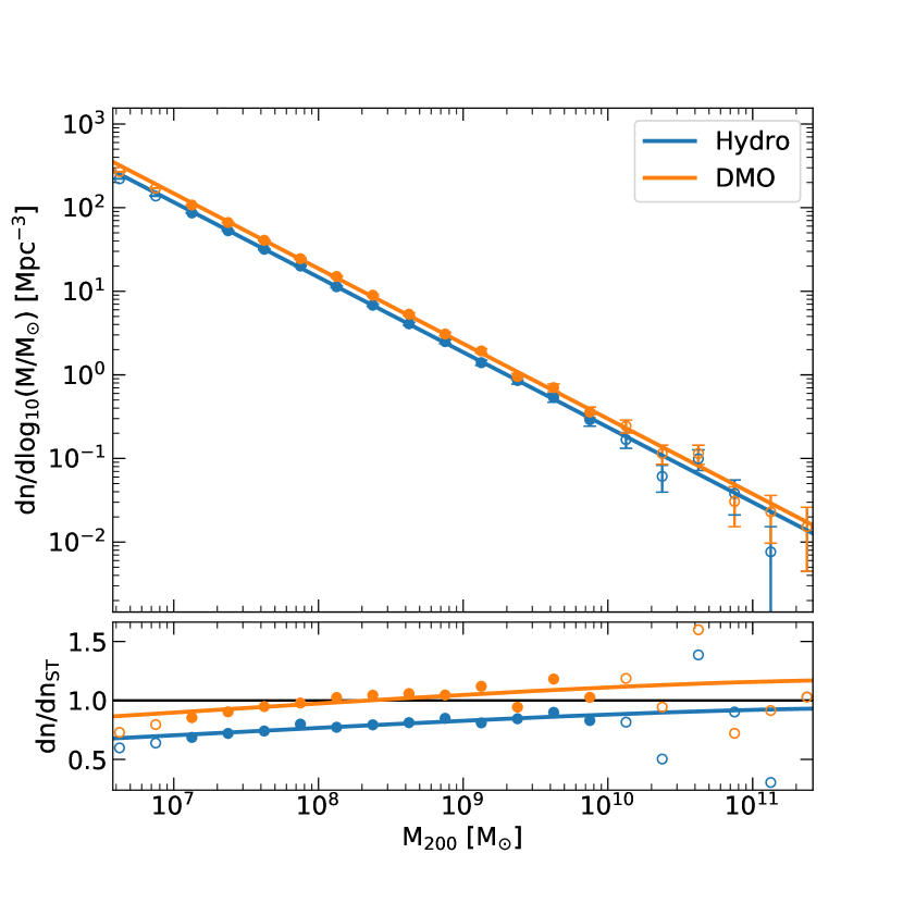
Figure 5: Top panel: the differential mass function of field halos in the hydrodynamical and DMO versions of our simulation, shown in blue and orange respectively. The mass function is calculated in a sphere of radius 5 Mpc centred on the potential minimum of the most massive halo in the high resolution region of the simulation. Circles show the measured halo mass function in each mass bin. The errorbars show the Poisson error. Solid lines show power-law fits to the halo mass function. Points shown with empty circles were not used when calculating the power-law fit. Bottom panel: the ratio of the calculated halo mass function to the analytic Sheth-Tormen mass function.

Our simulation contains a large enough field volume to allow us to study the abundance of the low-mass halos important for lensing. Fig. 5 shows the measured halo mass function in both the hydrodynamical and DMO versions of our simulation at redshift $z=0$. We find that the mass functions in both versions of the simulation are well fit by a power law, of the form,

$$\frac{\mathrm{d}n}{\mathrm{dlog_{10}}M/M_{\odot}}=b(M/M_{\odot})^{-a}\;,$$ (1)

in the range ($3\times 10^{6}$ – $3\times 10^{11}$) M_⊙. The best fit parameters are listed in Table 2. We find no significant difference between the slope of the halo mass functions in the hydrodynamical and DMO versions of our simulation. Across all halo masses considered, the amplitude of the DMO mass function is greater than the amplitude of the hydrodynamical mass function by around 25%. Given the mass function is a power-law with a slope of approximately -1, this difference is equivalent to all halos in the DMO simulation having their mass reduced by approximately 25%, consistent with the reduction in halo mass (at low halo masses) going from DMO to Eagle shown in Schaller et al. (2015).

The reduction in halo mass is caused by two processes operating at early times. Firstly, after the primordial gas is reionized, photo-heating evaporates gas from small mass halos or prevents it from cooling into them. Secondly, in halos where gas does cool and make stars supernovae expel the remaining gas (Benson et al., 2002; Benitez-Llambay & Frenk, 2020, and references therein). Of course, these processes are not modelled in DMO simulations and DMO halos become around 15% more massive (the value of $\Omega_{\mathrm{b}}/\Omega_{\mathrm{m}}$) than an otherwise equivalent halo in a hydrodynamical simulation. The loss of mass from these processes reduces the rate at which halos grow in the hydrodynamical simulation and the 15% difference at the redshift of reionisation increases to the 25% mass difference in halo mass at the present day (Sawala et al., 2016).

The measured slope of the halo mass function is shallower than the slope of the Sheth-Tormen mass function — 0.90 in the simulation and 0.92 in the Sheth-Tormen model. We can see in the lower panel of Fig. 5 that the Sheth-Tormen model overpredicts the abundance of halos less massive than $10^{10}$ M_⊙ in our high-resolution volume. While the difference in abundance between the Sheth-Tormen prediction and the DMO simulation could be affected by the special nature of the volume we have simulated, the difference in slope seems to be robust, as is the difference between the DMO and hydrodynamical simulation. We therefore conclude that previous studies which used the Sheth-Tormen model, e.g. Li et al. (2017), may have overpredicted the expected lensing signal originating from halos in the $10^{7}$–$10^{8}$ M_⊙ range by around 20–30%. Whilst we are unable to check whether the same overprediction applies to the calculation of the lensing signal in a WDM cosmology, this difference in the expected abundance of halos in a CDM universe is important from an observational standpoint.

	$a$	$b$ [Mpc-3]
Hydro	$0.897\pm 0.005$	$2.2\pm 0.2\times 10^{8}$
DMO	$0.898\pm 0.009$	$2.8\pm 0.5\times 10^{8}$

Table 2: Slope and amplitude of power-law fits to the halo mass function in the high-resolution region of our simulation at redshift $z=0$.

3.3 The effect of environment on the halo mass function

We also study the effect of environment on the abundance and properties of field halos. We use the Nexus code (Cautun et al., 2013) to classify halo environments. Nexus divides space into a cubic grid, and classifies each cell as belonging to either a void, a sheet, a filament, or a node. The method is scale-free, analysing the density field smoothed on a number of different scales in order to detect structure of all sizes.

The mass function of halos in voids, sheets and filaments is shown in the left-hand panel of Fig. 6. The slope of the mass function does not depend strongly on halo environment, but the amplitude of the mass function in different environments is strongly correlated with the average density of those environments; the amplitude of the halo mass function in filaments is an order of magnitude greater than in voids. It is natural to wonder whether the difference in amplitude results solely from the difference in the density of matter in each region. To account for the differing densities in each environment type, we also calculate the halo mass function per unit Lagrangian volume. The results are shown in the right-hand panel of Fig. 6. We see here that relative to the density of matter in each region, halos in the mass range considered here are less abundant in filaments than in voids. The halo masses we consider all lie comfortably below the characteristic clustering mass scale, $M^{\star}(z)$, which at redshift $z=0$ is around $6\times 10^{12}$ M_⊙ (White et al., 1993; Schneider et al., 2012b). The abundance of halos of a fixed mass below $M^{\star}(z)$ eventually decreases in time, as these smaller halos merge and accrete material to become larger halos. The higher density filament regions are effectively in a more advanced state of cosmic evolution relative to the lower density void regions, so the abundance of halos less massive than $M^{\star}(z)$ ends up lower in the filaments.

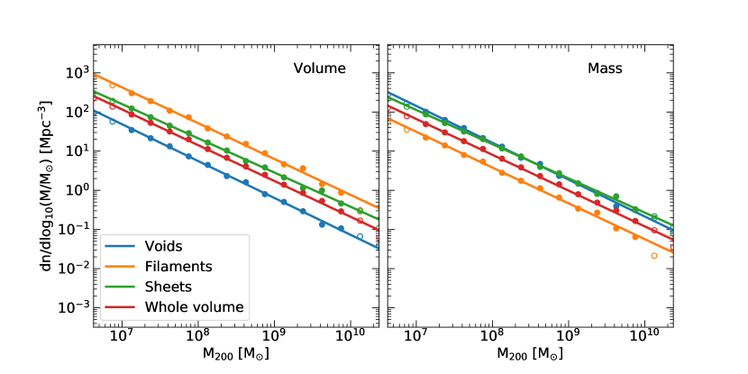
Figure 6: The differential halo mass function for halos in voids (blue), filaments (orange), sheets (green), and the entire volume (red) in the high-resolution region of the hydrodynamical version of our simulation at redshift $z=0$. The environment of a halo is determined using the Nexus algorithm (Cautun et al., 2013). Circles show the measured mass function, whilst lines show power-law fits. In the left-hand panel the amplitude of the mass function is normalised to the physical volume of each environment type. Empty circles show points not used when calculating power-law fits. In the right-hand panel the amplitude is normalised to the Lagrangian volume of each environment type, i.e the mass contained in each environment type.

3.4 The effect of environment on the internal structure of halos

We also consider the relationship between halo environment and the internal structure of the halo. Specifically, we compare the concentrations of halos in voids and filaments, for halo masses between $10^{7.5}$–$10^{9.5}$ M_⊙. If the halo has an NFW density profile (Navarro et al., 1996, 1997), with scale radius, $r_{\mathrm{s}}$, the concentration, $c$, is given by $r_{200}/r_{\mathrm{s}}$. We only consider halos which satisfy the three relaxation criteria of Neto et al. (2007), and where $r_{\mathrm{s}}$ is greater than the convergence radius of the halo, as defined using the criterion of Power et al. (2003). The distribution of concentrations for halos in the mass range $10^{7.5}$–$10^{9.5}$ M_⊙ at redshift $z=0$ is shown in Fig. 7.

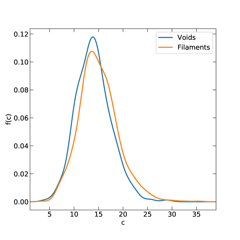
Figure 7: The distribution of concentration for halos in filaments and voids in the hydrodynamical version of our simulation at redshift $z=0$. Halos are selected to have masses between $10^{7.5}$–$10^{9.5}$ M_⊙. All halos in our sample satisfy the three relaxation criteria of Neto et al. (2007), and the concentrations are calculated by fitting NFW profiles.

Whilst the width and skew of the distribution is similar in both filaments and voids, we see that halos in filaments tend to have slightly higher concentrations, and halos with a concentration greater than 25 reside exclusively in filaments. The concentration of a halo reflects the density of the universe at its formation time Navarro et al. (1997). For a fixed mass, halos tend to form earlier in filaments than voids (Hahn et al., 2007), when the universe was denser. This explains the higher average concentration observed for halos in filaments.

4 The subhalo population

The small dark matter particle mass of our simulation allows us to study the abundance and properties of subhalos as small as $10^{7}$ M_⊙. This is the first time that such small substructures have been studied in a hydrodynamic simulation of a $10^{13}$ M_⊙ halo. In this section we focus on how the inclusion of baryons in the simulation changes the abundance and properties of this subhalo population.

For low-redshift halos of mass ${\sim}10^{13}$ M_⊙, a significant fraction of the distortions to strong lensing arcs is due to substructure within the lensing halo. For example, for a typical SLACS lens (at $z=0.2$, with a source at $z=1$), CDM substructure produces around 30% of the lensing distortions, whilst in WDM the contribution of substructures is comparable to that from field halos along the line-of-sight (Li et al., 2017; Despali et al., 2018).

4.1 The subhalo mass function

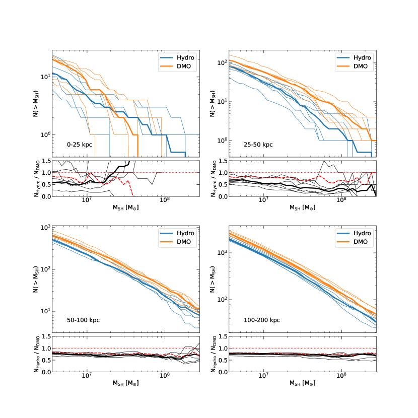
Figure 8: Large panels: cumulative subhalo mass functions in concentric spherical shells centred on the potential minimum of the central halo. Thin lines show the abundance of subhalos at six individual snapshots, approximately evenly spaced in time between redshift $z=0.5$ and the present day. Thick lines show the abundance of subhaloes averaged over these six snapshots. Small panels: the ratio of the cumulative subhalo mass functions in the hydrodynamical and DMO versions of the simulation at each snapshot (thin black lines). The thick black lines show the average reduction in subhalo abundance as a function of mass over a 5 Gyr period. The dashed red lines show the reduction in subhalo abundance when the masses of the objects in the DMO simulation are multiplied by 0.75 to approximate the reduced-growth effect described in §3.2.

Fig. 8 shows the cumulative subhalo mass function in four concentric spherical shells centred on the potential minimum of the halo. We see that the inclusion of baryons in the simulation leads to a reduction in subhalo abundance as a function of subhalo mass. As discussed in §3.2, halos in cosmological hydrodynamical simulations are systematically less massive than their DMO counterparts because the loss of baryons at early time reduces their subsequent growth rate. To distinguish this “reduced-growth” effect from environmental effects, such as tidal stripping and disruption, we apply a correction to the subhalo abundance in the DMO simulation by reducing the masses by 25%, which is the typical size of the reduced-growth effect. The corresponding reduction in subhalo abundance is shown by the red dotted line in each panel.

In the innermost radial bin, the total number of subhalos in the mass range $(3\times 10^{6}-3\times 10^{7})$ M_⊙ is reduced by around 50%, although there is considerable scatter in the different snapshots. Approximately half the measured reduction is due to dynamical processes – tidal stripping and destruction – and half to the reduced-growth effect. The average reduction in subhalo abundance in this region is comparable to that in Milky Way-mass halos found in the Apostle simulations, which also used the Eagle model (Richings et al., 2020). This is not surprising as the ratio of galaxy to halo mass is similar in all these simulations.

There is a clear radial trend in the reduction of subhalo abundance in the hydrodynamical simulation. The effect of the central galaxy on the subhalo population is negligible at distances greater than 100 kpc (which is also the case in the Apostle simulations). Here, the reduction is essentially independent of subhalo mass and is explained entirely by the reduced-growth effect in hydrodynamical simulation. In the inner shells, where the effect of the central galaxy is important, there seems to be some dependence of the reduction on subhalo mass but the numbers are too small to reach a firm conclusion.

4.2 Subhalo concentrations

Since the size of a subhalo is not well defined, it is better to characterise their concentrations in terms of their mean overdensity, $\delta_{V}$, within the radius, $r_{\mathrm{max}}$, at which the circular velocity peaks, in units of the critical density,

$$\delta_{V}=2\left(\frac{V_{\mathrm{max}}}{H_{0}r_{\mathrm{max}}}\right)^{2}\;,$$ (2)

where $V_{\mathrm{max}}$ is the maximum circular velocity of the halo Springel et al. (2008). For an NFW halo, the concentration, $c$, is related to $\delta_{V}$ by

$$\delta_{V}=7.213\left(\frac{200}{3}\right)\frac{c^{3}}{\ln(1+c)-c/(1+c)}\;.$$ (3)

Whilst this equation cannot be inverted analytically, we find that an approximate relation that holds well for concentrations between 5 and 50 is

$$c=0.3\delta_{V}^{0.4}\;.$$ (4)

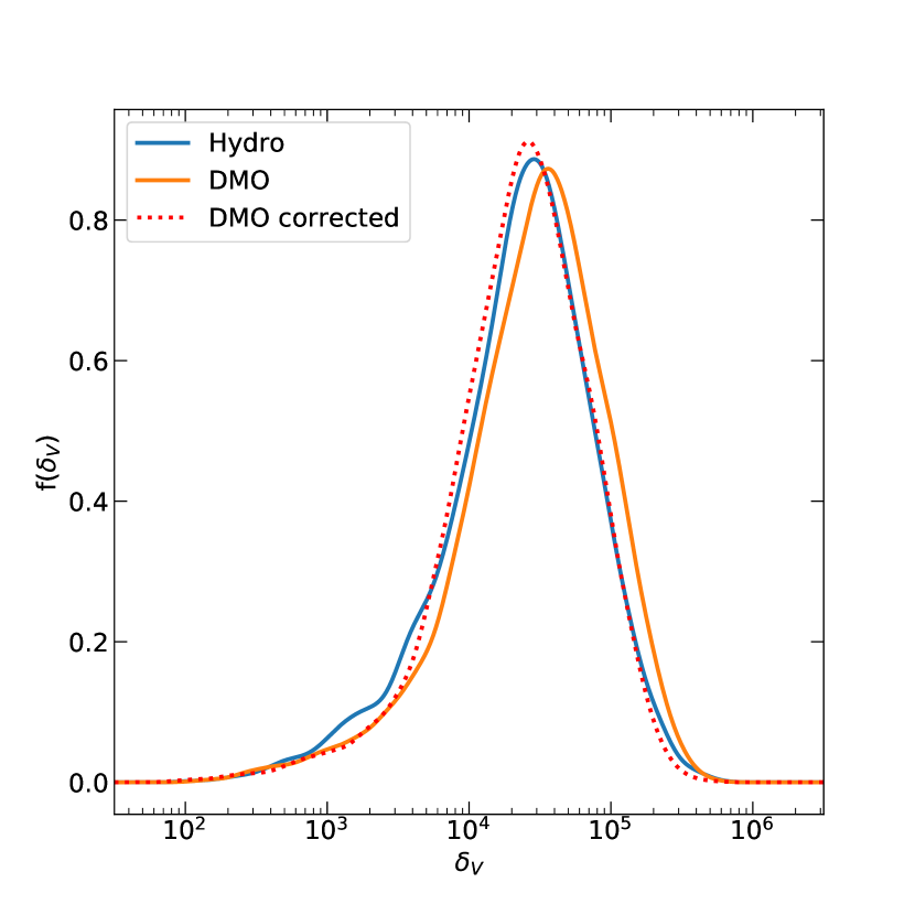
Figure 9: The distribution of subhalo characteristic overdensity, $\delta_{V}$ (which we use to characterize subhalo concentration) in the hydrodynamical and DMO versions of our simulation at redshift $z=0$. Subhalos are selected to have maximum circular velocities between 3 and 20 km/s. The dotted red line corresponds to the case when the DMO $V_{\mathrm{max}}$ values are multiplied by 0.85 to account for the systematic mass difference between hydrodynamical and DMO halos due to the reduced-growth effect discussed in §3.2.

The distribution of $\delta_{V}$ for subhalos with $V_{\mathrm{max}}$ between 3 and 20 km/s lying within 500 kpc of the centre of the main halo at $z=0$ is shown in Fig. 9. We only consider well-resolved subhalos by requiring that $r_{\mathrm{max}}$ be greater than the gravitational softening length, 0.5 kpc. Subhalos in the hydrodynamical version of our simulation are systematically less concentrated than subhalos in the DMO version, although the difference is small. The peak of the DMO distribution occurs at a value of $\delta_{V}$ which is 23% higher than in the hydrodynamical simulation. The difference in $\delta_{V}$ is equivalent to a difference of approximately 8% in concentration for NFW halos. Fig. 9 also shows the distribution of $\delta_{V}$ for subhalos in the DMO simulation when the values of $V_{\mathrm{max}}$ are reduced by 15% to mimic the reduced-growth effect discussed in §3.2, as found by Sawala et al. (2016) for field halos. This slight shift in $V_{\mathrm{max}}$ largely explains the difference between the hydrodynamics and DMO distributions. We conclude that the inclusion of baryons in the simulations does not have a significant impact on the concentration of subhalos in the mass range considered, beyond a small shift.

4.3 Projection effects

The projected mass distribution is responsible for gravitational lensing and, since the spatial distribution of mass around a large halo is strongly anisotropic, the observed lensing effect will depend on the direction along which the lens is observed. The central halo in our simulation sits at the intersection of three filaments (see Fig. 4). The number density of substructures along these filaments is greater than the average around the halo, so a lens observed along a a filament will be affected by substructure much more strongly than a lens observed along an average direction.

A visual representation of the dependence of the observed abundance of substructure on viewing angle is presented in Fig. 10. To construct this image we distributed $10^{6}$ lines-of-sight uniformly on the surface of a sphere centred on the potential minimum of the main halo. Along each line-of-sight, we calculate the number of halos and subhalos with a Subfind mass between $10^{6.5}$–10^8.5 M_⊙, in a cylinder of radius 10 kpc and length 10 Mpc centred on the main halo. This includes the subhalos of the main halo, and also other halos and their subhalos which fall along the line-of-sight. The map of the number of objects along each line-of-sight in Fig. 10 is smoothed on a scale of one degree and is for the cluster at redshift $z=0.1$ since this is typical of low-redshift lenses (e.g. Bolton et al., 2006) and is the value used in the analysis of Li et al. (2017).

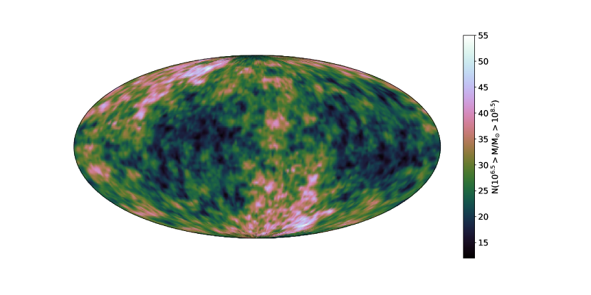
Figure 10: The number of halos and subhalos of mass in the range $(10^{6.5}$–$10^{8.5})$ M_⊙ along lines-of-sight to the main cluster in the hydrodynamical simulation at redshift $z=0.1$. Each line-of-sight is a cylinder of 10 Mpc length and 10 kpc radius. The map is an equal-area Mollweide projection, smoothed on a scale of one degree, made from $10^{6}$ lines-of-sight spread almost uniformly across the surface of a sphere of radius 5 Mpc centred on the main halo.

It is clear that the number of objects varies strongly with viewing angle. Highly populated viewing angles are closely aligned with filaments and often contain 2–3 times as many objects as viewing angles that do not overlap a filament. The dominant contribution to the signal originates from subhalos, not from nearby field halos although the distinction between halos and subhalos is ambiguous as the shape of the halo, and thus the number of subhalos along a particular line-of-sight, is strongly correlated with the direction of the filaments. From an observational perspective, the distinction is artificial.

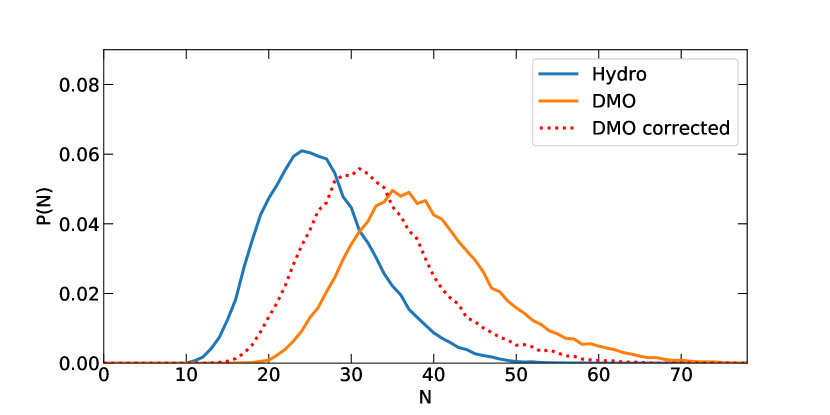
Figure 11: The distribution of the number of halos and subhalos of mass between $10^{6.5}$–$10^{8.5}$ M_⊙ along lines-of-sight projected through the centre of the main halo at redshift $z=0.1$. Each projection is of a cylinder of 10 Mpc length and 10 kpc radius. The dotted red line shows the distribution in the case where the masses of all objects in the DMO version of our simulation are multiplied by 0.75 to account for the effect discussed in §3.2.

We compare the distribution of the number of objects along different lines-of-sight in the hydrodynamical and DMO versions of our simulation in Fig. 11. The median number of objects along a line-of-sight, and the interquartile ranges, are listed in Table 3. The number of objects along a given line-of-sight in the hydrodynamical simulation is around 30% smaller on average. This is a combination of the reduced-growth effect together with the destruction and tidal stripping of subhalos in the hydrodynamical simulation. Comparison of the abundance in the hydrodynamical simulation to that in the DMO simulation with the masses of objects reduced by 25% (dotted red line) shows that the reduced-growth effect accounts for approximately half of the measured difference between the hydrodynamical and DMO simulations. In the hydrodynamical simulation, the median number of objects along the line of sight is 26, but there are lines-of-sight that intercept more than twice this number.

Simulation	N
Hydro	$26^{+5}_{-4}$
DMO	$38^{+5}_{-5}$
DMO - corrected	$32^{+5}_{-5}$

Table 3: The median number of objects in the mass range $(10^{6.5}$–$10^{8.5})$ M_⊙ along a 10 Mpc long cylindrical line-of-sight of radius 10 kpc centred on the potential minimum of the main halo. Subscripts and superscripts give the interquartile range. The numbers quoted includes subhalos of the main halo as well as field halos.

5 Conclusions

We have developed a new technique to generate initial conditions for cosmological smooth particle hydrodynamics simulations in which the number of dark matter particles can be much larger than the number of gas particles. Our main motivation is to simulate a massive elliptical galaxy with realistic galaxy formation astrophysics – which requires good gas resolution – while, at the same time, resolving the $\sim 10^{6}$ M_⊙ haloes and subhaloes relevant to strong gravitational lensing tests of the identity of the dark matter – which requires very high dark matter resolution. An added benefit of our new technique is that it avoids the 2-body scattering processes inherent in the traditional cosmolgical SPH setup in which the dark matter and the gas are followed with the same number of particles which, consequently have very different masses (Ludlow et al., 2019).

We have simulated a $10^{13}$M_⊙ galaxy cluster and its surrounding large-scale environment, a volume of over 500 Mpc³, using the Eagle Reference model of galaxy formation. Our conclusions may be summarized as follows:

$\bullet$ The field halo mass function in the mass range ($5\times 10^{6}-3\times 10^{11}$) M_⊙ closely follows a power law of slope -0.9 in both the DMO and hydrodynamic simulations (see Table 2). However, the amplitude of the halo mass function in the hydrodynamics case is about 25% lower than in the DMO case (Fig. 5). The difference originates at early times when halos in the hydrodynamics simulation lose gas, either as a result of reionization or of supernovae feedback and, as a result, experience less growth than their DMO counterparts, as first discussed by Sawala et al. (2016).

$\bullet$ The halo mass functions are not well described by the commonly used Sheth-Tormen formula, which is based on a fit to DMO simulations and has a steeper slope than we measure. As a result, previous lensing studies using the Sheth-Tormen model have overpredicted the expected lensing signal originating from halos in the ($10^{7}$–$10^{8}$) M_⊙ range by around 20–30%.

$\bullet$ The abundance of field halos depends sensitively on environment. In our hydrodynamical simulation we find that the number of halos per unit mass in the range of halo masses considered here is largest in the sheets and voids of the cosmic web, where it exceeds the number per unit mass in filaments by a factor of four to five (although the volume-weighted number is largest in filaments; Fig. 6).

$\bullet$ The mass function of subhalos in the cluster also has lower amplitude in the hydrodynamical simulation than in the DMO simulation (Fig. 8). In addition to the same reduced growth experienced by field halos, the subhalo abundance is further reduced in the hydrodynamical simulation by the enhanced destruction of subhalos caused by the stronger tidal interactions in the presence of a massive galaxy at the centre of the cluster. The extent of this destruction depends sensitively on radius. For example, within 50 kpc in projection, the number of substructures in the ($10^{6.5}$–$10^{8.5}$) M_⊙ mass range in the hydrodynamics simulation is only about half the number in the DMO simulation (with considerable halo-to-halo scatter). Approximately 50% of this difference is accounted for by the reduced growth effect in the hydrodynamical simulation and the remaining 50% by tidal disruption. Beyond 100 kpc from the centre, the effect of the central galaxy is small and the reduction is due almost entirely to the reduced-growth effect.

$\bullet$ Subhalos in the hydrodynamical simulation are less concentrated than their DMO counterparts but the difference is only about 10%. It arises from the reduced-growth effect which effectively shifts the formation time of halos in the hydrodynamical simulation to slightly later times.

$\bullet$ The matter distribution around the cluster is highly anisotropic and, as a result, the projected number of halos and subhalos – the quantity of interest in strong gravitational lensing studies – is also highly anisotropic. For example, the projected number of objects in the mass range ($10^{6.6}-10^{8.5}$) M_⊙ along a cylinder of radius 10 kpc and length 10 Mpc centred on cluster can be 2-3 times larger if aligned with a filament than if not.

The analysis of the perturbations on strong gravitational lenses offers a real prospect of testing the $\Lambda$CDM model in the regime of small-mass halos where it makes robust predictions that distinguish it from viable alternatives such as WDM (Li et al., 2017). The prime targets for this kind of lensing studies are $10^{13}$ M_⊙ halos like the one we have simulated here. Understanding the abundance, structure and distribution of subhalos in these halos, and of field halos around them, is an important prerequisite for the successful application of lensing techniques to the problem of the identity of the dark matter.

Data availability

The data underlying this article will be shared on reasonable request to the corresponding author.

References

- Bahé et al. (2017) Bahé Y. M., et al., 2017, MNRAS, 470, 4186
- Benitez-Llambay & Frenk (2020) Benitez-Llambay A., Frenk C., 2020, arXiv e-prints, p. arXiv:2004.06124
- Benson et al. (2002) Benson A. J., Frenk C. S., Sharples R. M., 2002, ApJ, 574, 104
- Bode et al. (2001) Bode P., Ostriker J. P., Turok N., 2001, ApJ, 556, 93
- Bolton et al. (2006) Bolton A. S., Burles S., Koopmans L. V. E., Treu T., Moustakas L. A., 2006, ApJ, 638, 703
- Bolton et al. (2008) Bolton A. S., Burles S., Koopmans L. V. E., Treu T., Gavazzi R., Moustakas L. A., Wayth R., Schlegel D. J., 2008, ApJ, 682, 964
- Bose et al. (2017) Bose S., et al., 2017, MNRAS, 464, 4520
- Boyarsky et al. (2014) Boyarsky A., Ruchayskiy O., Iakubovskyi D., Franse J., 2014, Physical Review Letters, 113, 251301
- Bulbul et al. (2014) Bulbul E., Markevitch M., Foster A., Smith R. K., Loewenstein M., Randall S. W., 2014, ApJ, 789, 13
- Cautun et al. (2013) Cautun M., van de Weygaert R., Jones B. J. T., 2013, MNRAS, 429, 1286
- Colín et al. (2000) Colín P., Avila-Reese V., Valenzuela O., 2000, ApJ, 542, 622
- Crain et al. (2015) Crain R. A., et al., 2015, MNRAS, 450, 1937
- D’Onghia et al. (2010) D’Onghia E., Springel V., Hernquist L., Keres D., 2010, ApJ, 709, 1138
- Davis et al. (1985) Davis M., Efstathiou G., Frenk C. S., White S. D. M., 1985, ApJ, 292, 371
- Despali & Vegetti (2017) Despali G., Vegetti S., 2017, MNRAS, 469, 1997
- Despali et al. (2016) Despali G., Giocoli C., Angulo R. E., Tormen G., Sheth R. K., Baso G., Moscardini L., 2016, MNRAS, 456, 2486
- Despali et al. (2018) Despali G., Vegetti S., White S. D. M., Giocoli C., van den Bosch F. C., 2018, MNRAS, 475, 5424
- Diemand et al. (2007) Diemand J., Kuhlen M., Madau P., 2007, ApJ, 667, 859
- Frenk et al. (1983) Frenk C. S., White S. D. M., Davis M., 1983, ApJ, 271, 417
- Frenk et al. (1996) Frenk C. S., Evrard A. E., White S. D. M., Summers F. J., 1996, ApJ, 472, 460
- Garrison-Kimmel et al. (2017) Garrison-Kimmel S., et al., 2017, preprint, (arXiv:1701.03792)
- Gilman et al. (2020) Gilman D., Birrer S., Nierenberg A., Treu T., Du X., Benson A., 2020, MNRAS, 491, 6077
- Grand et al. (2016) Grand R. J. J., Springel V., Gómez F. A., Marinacci F., Pakmor R., Campbell D. J. R., Jenkins A., 2016, MNRAS, 459, 199
- Hahn et al. (2007) Hahn O., Carollo C. M., Porciani C., Dekel A., 2007, MNRAS, 381, 41
- Hellwing et al. (2016) Hellwing W. A., Frenk C. S., Cautun M., Bose S., Helly J., Jenkins A., Sawala T., Cytowski M., 2016, MNRAS, 457, 3492
- Jenkins et al. (2001) Jenkins A., Frenk C. S., White S. D. M., Colberg J. M., Cole S., Evrard A. E., Couchman H. M. P., Yoshida N., 2001, MNRAS, 321, 372
- Jiang et al. (2014) Jiang L., Helly J. C., Cole S., Frenk C. S., 2014, MNRAS, 440, 2115
- Kegerreis et al. (2019) Kegerreis J. A., Eke V. R., Gonnet P. G., Korycansky D. G., Massey R. J., Schaller M., Teodoro L. F. A., 2019, arXiv e-prints, p. arXiv:1901.09934
- Kennedy et al. (2014) Kennedy R., Frenk C., Cole S., Benson A., 2014, MNRAS, 442, 2487
- Koopmans (2005) Koopmans L. V. E., 2005, MNRAS, 363, 1136
- Li et al. (2017) Li R., Frenk C. S., Cole S., Wang Q., Gao L., 2017, MNRAS, 468, 1426
- Lovell et al. (2012) Lovell M. R., et al., 2012, MNRAS, 420, 2318
- Lovell et al. (2017) Lovell M. R., Gonzalez-Perez V., Bose S., Boyarsky A., Cole S., Frenk C. S., Ruchayskiy O., 2017, MNRAS, 468, 2836
- Lovell et al. (2018) Lovell M. R., et al., 2018, MNRAS, 481, 1950
- Ludlow et al. (2019) Ludlow A. D., Schaye J., Schaller M., Richings J., 2019, MNRAS, 488, L123
- Massey et al. (2010) Massey R., Kitching T., Richard J., 2010, Reports on Progress in Physics, 73, 086901
- Navarro et al. (1996) Navarro J. F., Frenk C. S., White S. D. M., 1996, ApJ, 462, 563
- Navarro et al. (1997) Navarro J. F., Frenk C. S., White S. D. M., 1997, ApJ, 490, 493
- Neto et al. (2007) Neto A. F., et al., 2007, MNRAS, 381, 1450
- Planck Collaboration et al. (2014) Planck Collaboration et al., 2014, A&A, 571, A1
- Planck Collaboration et al. (2016) Planck Collaboration et al., 2016, A&A, 596, A108
- Power et al. (2003) Power C., Navarro J. F., Jenkins A., Frenk C. S., White S. D. M., Springel V., Stadel J., Quinn T., 2003, MNRAS, 338, 14
- Richings et al. (2020) Richings J., et al., 2020, MNRAS, 492, 5780
- Rodríguez-Torres et al. (2016) Rodríguez-Torres S. A., et al., 2016, Monthly Notices of the Royal Astronomical Society, 460, 1173
- Saff & Kuijlaars (1997) Saff E. B., Kuijlaars A. B. J., 1997, The Mathematical Intelligencer, 19, 5
- Sawala et al. (2013) Sawala T., Frenk C. S., Crain R. A., Jenkins A., Schaye J., Theuns T., Zavala J., 2013, MNRAS, 431, 1366
- Sawala et al. (2016) Sawala T., et al., 2016, MNRAS, 457, 1931
- Sawala et al. (2017) Sawala T., Pihajoki P., Johansson P. H., Frenk C. S., Navarro J. F., Oman K. A., White S. D. M., 2017, MNRAS, 467, 4383
- Schaller et al. (2015) Schaller M., et al., 2015, MNRAS, 451, 1247
- Schaye et al. (2015) Schaye J., et al., 2015, MNRAS, 446, 521
- Schneider et al. (2012a) Schneider A., Smith R. E., Macciò A. V., Moore B., 2012a, MNRAS, 424, 684
- Schneider et al. (2012b) Schneider M. D., Frenk C. S., Cole S., 2012b, J. Cosmology Astropart. Phys., 2012, 030
- Schneider et al. (2013) Schneider A., Smith R. E., Reed D., 2013, MNRAS, 433, 1573
- Sheth & Tormen (2002) Sheth R. K., Tormen G., 2002, MNRAS, 329, 61
- Springel et al. (2001) Springel V., White S. D. M., Tormen G., Kauffmann G., 2001, MNRAS, 328, 726
- Springel et al. (2005) Springel V., et al., 2005, Nature, 435, 629
- Springel et al. (2008) Springel V., et al., 2008, MNRAS, 391, 1685
- Tinker et al. (2008) Tinker J., Kravtsov A. V., Klypin A., Abazajian K., Warren M., Yepes G., Gottlöber S., Holz D. E., 2008, The Astrophysical Journal, 688, 709
- Vegetti et al. (2012) Vegetti S., Lagattuta D. J., McKean J. P., Auger M. W., Fassnacht C. D., Koopmans L. V. E., 2012, Nature, 481, 341
- White et al. (1983) White S. D. M., Frenk C. S., Davis M., 1983, ApJ, 274, L1
- White et al. (1984) White S. D. M., Davis M., Frenk C. S., 1984, MNRAS, 209, 27P
- White et al. (1993) White S. D. M., Efstathiou G., Frenk C. S., 1993, MNRAS, 262, 1023
- Zel’dovich (1970) Zel’dovich Y. B., 1970, A&A, 5, 84