Arnoldi algorithms with structured orthogonalization

Abstract

We study a stability preserved Arnoldi algorithm for matrix exponential in the time domain simulation of large-scale power delivery networks (PDN), which are formulated as semi-explicit differential algebraic equations (DAEs). The solution can be decomposed to a sum of two projections, one in the range of the system operator and the other in its null space. The range projection can be computed with one shift-and -invert Krylov subspace method. The other projection can be computed with the algebraic equations. Differing from the ordinary Arnoldi method, the orthogonality in the Krylov subspace is replaced with the semi-inner product induced by the positive semi-definite system operator. With proper adjustment, numerical ranges of the Krylov operator lie in the right half plane, and we obtain theoretical convergence analysis for the modified Arnoldi algorithm in computing phi-functions. Lastly, simulations on RLC networks are demonstrated to validate the effectiveness of the Arnoldi algorithm with structured-orthogonalization.

1 Introduction

Evaluating the performance of a power deliver network (PDN) has become a critical issue in very large-scale integration (VLSI) designs. The power supply from the package down to on-chip integrated circuits is distributed through metal layers and vias, which could be modeled as a linear network consisting of resistors, capacitors and inductors [Nas08]. The on-chip circuit modules are simplified as time-varying current sources in PDN analysis. Due to the shrinking feature size and increasing design complexity, the network could easily consist of millions to billions of elements which result in an extremely huge system. Moreover, the values of elements in a system level PDN may vary greatly and the transient responses include many different scaled time constants, which makes the whole differential system very stiff. In order to characterize the long term dynamic behavior, an extended time span at small-scaled time steps is necessary and extra computation efforts are required. At the same time, the stiffness of the system is increased which degrades the performance of traditional simulation methods. All the challenges make a fast and accurate simulator in high demand.

Let $x(t)\in\mathbb{R}^{N}$ be the solution to a system of stiff differential equations,[CCPW18, WCC19]

$$\frac{dq(t)}{dt}+f(x(t))=u(t),\;x(0)=x_{0},$$ (1)

where $u(t)$ is the input signal to the circuit system, $x(t)\in\mathbb{R}^{N}$ of large dimension $N$ denotes nodal voltages and branch currents at time $t$ and $q,f\in\mathbb{R}^{N}$ are the charge(or flux) and current (or voltage) terms, respectively. The system is governed by Kirchhoff’s current law and voltage law. With linearization, we have

$$C\frac{dx}{dt}+Gx=u(t),x(0)=x_{0},$$ (2)

where $C$ and $G$ both are $N\times N$ matrices, which are the Jacobian matrices of $q$ and $f$ with respect to $x$, respectively. In the study, we assume that $C,G$ are constant matrices and

$$\begin{cases}&\textrm{ $G$ is positive definite, but not necessarily symmetric};\\ &\textrm{ $C$ is positive semi-definite and symmetric. }\end{cases}$$ (3)

Every node is supposed to connect to power or ground via a path of resistors, which makes $G$ nonsingular. For a stiff system, the solution can be of multiple timescales, i.e., the attractive solution is surrounded with fast-changing nearby solutions.

When $C$ is nonsingular, the solution can be formulated as exponentials of the matrix $A:=C^{-1}G$. There are various ways to implement the computation[MVL78],[MVL03] depending on the state companion matrix $A$. When $A$ is a matrix in small size, the most effective algorithm is a scaling-and-squaring method based on Padé approximation[Tre12]. When $A$ is sparse and large, one general and well-established technique is approximating the action of the matrix exponentials in the class of Krylov subspaces. One essential ingredient is the evaluation or approximation of the product of the exponential of the Jacobian $A$ with a vector $v$. The application of Krylov subspace techniques has been actively investigated in the literatures[FTDR89, Saa92, MVL03, HOS09, NW12, JdlCM20]. In general, the nonlinear form in (1) can be numerically handled by various exponential Runge-Kutta schemes with the aid of exponential integrators[HOS09, HO10] and references therein.

It is well-known that Krylov subspace methods for matrix functions exhibits super-linear convergence behavior under sufficient large Krylov dimension (larger than the norm of the operator)[Saa92][HL97]. Recently, researchers observe the superiority of rational Krylov subspace methods over standard Krylov subspace methods, in particular, the spectrum of the operator lies in the half-plane, e.g., the Laplacian operators in PDEs[DK98],[GH08]. The convergence of computing exponential integrators of evolution equations in the resolvent Krylov subspace is independent of the operator norm of $A$ from one numerical discretization, when $A$ in $\exp(-A)$ has numerical range(or called field of values) in the right half plane [Gri12][GG17].

Exponential integrator based methods have been introduced for PDN transient simulations [ZYW⁺16, CCPW18]. Compared to the traditional linear multi-step methods, the matrix exponential based method is not bounded by the Dahlquist stability barrier thus larger step size can be employed [Wan06, ZYW⁺16]. The stability of matrix exponential based method when applied to ODEs has been well established in previous work [WCC12, ZYW⁺16]. For general circuit simulation with DAEs, the stability remains an interesting topic [Fre00, IR14, Win03, TI10]. Numerical stability issues are reported in [CCPW18, WCC19] and reveal the limitation of matrix exponential computations with Krylov subspace. Similar problems occur in the eigenvalue computation [MS97, NOPEJ87] and model order reduction for interconnect simulation [RM09, MKEW96], where Krylov subspace methods are widely used. As one shift-and-invert method, one modified Arnoldi algorithm for matrix exponential are proposed to provide stable computations of matrix exponentials, where Arnoldi vectors are orthogonal with respect to the system operator $C$[CCPW18, WCC19].

In this paper, we shall examine the modified shift-and-invert Arnoldi algorithm from the perspective of numerical ranges, which provides one theoretical foundation for the Arnoldi algorithm described in [2018transient, WCC19]. Since the matrix $C$ could be singular in PDN transient simulation, we introduce $C$ semi-inner product as well as its induced norm,

$$\langle x,y\rangle_{C}:=\Re(x^{*}Cy),\;\|x\|_{C}:=\Re(x^{*}Cx)$$

to derive the error analysis, instead of the ordinary inner product $\langle x,y\rangle:=\Re(x^{*}y)$. Likewise, the $C$-norm $\|x\|_{C}:=\sqrt{x^{*}Cx}$ is used to define the so-called $C$-numerical ranges in (54). The advantage of $C$ semi-inner product introduced in the modified Arnoldi algorithm is two-fold: the null-space component is removed in the Arnoldi iterations and the $C$-numerical range of the operator in the matrix exponentials lies in the right half plane. The numerical range of the upper Hessenberg matrix is properly restricted within a disk with center at $1/2$ and radius $1/2$. The $C$ semi-inner product as well as the associated Arnoldi algorithm have been employed for different purposes, e.g, solving generalized eigenvector problems[Eri86, MS97] and generating stable and passive Arnoldi-based model order reduction[MKEW96].

The main contributions are listed as follows. With the aid of eigenvectors of $C$ as a basis, solutions $x(t)$ to PDNs can be decomposed to a sum of $x_{\mathcal{R}}(t)$ and $x_{\mathcal{N}}(t)$. The shift-and-invert Krylov method in [WCC19] computes $x_{\mathcal{R}}(t)$, which actually captures the dominant transient dynamical behaviors. The orthonormal basis of Krylov subspace is generated by a quadratic norm with the system matrix to preserve the passivity property of the system, which yields stable transient simulations. The positive definite matrix $G$ guarantees the $C$-numerical range of $G^{-1}C$ lying the right half plane, which establishes the convergence to $x_{\mathcal{R}}(t)$ as Krylov dimension tends to infinity, including posterior error bounds and prior error bounds. The shift parameter $\gamma$ in the shift-and-invert method provides the flexibility to confine the spectrum of ill-conditioned systems [ER80]. The error with $\varphi_{k}$-functions tends to $0$ as the dimension increases. In the case of $\varphi_{0}$ computation with $\gamma$ proportional to time step size, the error curve with respect to $\log\gamma$ is a $\cap$-shaped curve. The stagnation in the small $\gamma$ can be significantly improved, when the $\varphi_{1}$ or $\varphi_{2}$ computation is introduced, which is consistent with empirical studies reported in ([WCC19]).

The rest of this paper is organized as follows. The differential algebraic equations(DAEs) framework is introduced in Sec. 1.1. The explicit formulations of solutions in the basis of eigenvectors of $G^{-1}C$ and in the basis of eigenvectors of $C$ are given in section 1.2 and 1.3, respectively. In the paper, we focus on the computation of the projected solution $x_{\mathcal{R}}(t)$. In section 1.4, we introduce Krylov space corresponding to the shift-and invert method, which is used to approximate the solution. In section 2.2, we give a posterior error bound based on the residual errors and prior error bound. In section 3, we provide simulations on RLC networks with $G$ only positive semidefinite to validate the effectiveness of the modified shift-and-invert Arnoldi algorithm and examine the error behaviors in computing matrix exponentials.

1.1 Solutions of nonsingular systems

Suppose that $C$ is nonsingular with $A=C^{-1}G$. The variation-of-constants formula yields the solution $x(t)$ described by

$$x(t)=\exp(-tA)x_{0}+\int_{0}^{t}\exp(-(t-s)A)C^{-1}u(s)\,ds.$$ (4)

Introducing so-called phi-functions,

$$\varphi_{0}(z):=\exp(z),\;\varphi_{k+1}(z):=(\varphi_{k}(z)-(k!)^{-1})/z\textrm{ for $k\geq 0$ },$$ (5)

we can approximate (4) under linearization on the source term $C^{-1}u(s)\approx b+b^{\prime}s$ as a sum of the $\varphi_{0}$, $\varphi_{1}$ and $\varphi_{2}$ terms.

$$x(t+h)\approx\varphi_{0}(-hA)x(t)+h\varphi_{1}(-hA)b+h^{2}\varphi_{2}(-hA)b^{\prime},$$ (6)

where $\varphi_{0}(z)=\exp(z)$ and $\varphi_{1}(z)=z^{-1}(\exp(z)-1)$. One can employ the shift-and-invert Arnoldi transform to solve one nonsingular differential system as in ([BGH13]) Briefly, let $A=C^{-1}G$ and construct the Krylov subspace with respect to $(I+\gamma A)^{-1}$ with a parameter $\gamma>0$, i.e.,

$$(I+\gamma A^{-1})^{-1}V_{m}=V_{m+1}\widetilde{H}_{m},$$

where one orthogonal basis matrix $V_{m}\in\mathbb{R}^{N\times m}$ and one upper-Hessenburg matrix $\widetilde{H}_{m}\in\mathbb{R}^{(m+1)\times m}$ are generated. Let $H_{m}$ be the sub-matrix of $\widetilde{H}_{m}$ without the last row. Then the terms $\varphi_{0},\varphi_{1}$ in (4) can be approximated by the exponential function of $H_{m}$, e.g.,

$$\exp(-tA)x_{0}\approx\|x_{0}\|\exp(-\gamma t(H_{m}^{-1}-I_{m}))e_{1}.$$ (7)

1.2 Solutions of singular systems

A nonsingular matrix $C$ cannot always achieved in general power delivery networks. For instance, the nodes without nodal capacitance or inductance would contribute to the algebraic equations and the corresponding matrix $C$ is not invertible. One major impact from the singularity is that the system in (2) is in fact one combination of differential equations and algebraic equations, i.e., $x(t)$ must satisfy the range condition: $x(t)-G^{-1}u(t)$ in the range of $G^{-1}C$. In addition, since the projection $H_{m}$ is constructed from an initial vector, without careful and proper handling, the matrix $H_{m}$ could become a nearly degenerate matrix, and (7) boils down to be an erroneous approximation. Hence, it is natural to perform some proper decomposition on $x(t+h)$ based on nonzero and zero eigenvalues, so that $H_{m}$ is not contaminated by null vectors and the solution $x(t)$ can be computed accurately.

We discuss two decompositions to express the solutions. Start with the standard approach in differential equations. (This approach is listed as Method 16 in [MVL03].) Let $G^{-1}C=V\Lambda V^{-1}$ be the Joran canonical form decomposition of $G^{-1}C$, where

$$\Lambda=\left(\begin{array}[]{cc}J_{\mathcal{R}}&0\\ 0&J_{\mathcal{Z}}\end{array}\right)\in\mathbb{C}^{N\times N}$$

is in Jordan normal form. The submatrix $J_{\mathcal{R}}\in\mathbb{C}^{r\times r}$ consists of a few Jordan blocks corresponding to nonzero eigenvalues of $G^{-1}C$ and $J_{\mathcal{Z}}\in\mathbb{R}^{(N-r)\times(N-r)}$ is a nilpotent matrix corresponding to eigenvalue zero of $G^{-1}C$. Since the null space of $G^{-1}C$ has dimension $N-n$, the algebraic multiplicity of the eigenvalue zero is not less than $N-n$. Write $V=[V_{\mathcal{R}},V_{\mathcal{Z}}],\;V_{\mathcal{Z}}:=[V_{\mathcal{G}},V_{\mathcal{N}}]$, where columns of $V_{\mathcal{R}}$ and $V_{\mathcal{Z}}$ are the (generalized) eigenvectors of nonzero eigenvalues, respectively. Columns of $V_{\mathcal{G}}$ and $V_{\mathcal{N}}$ are the generalized eigenvectors and the eigenvectors of eigenvalue $0$. That is, columns of $V_{\mathcal{N}}$ are the null vectors of $G^{-1}C$. Let $U:=(V^{-1})^{*}=[U_{\mathcal{R}},U_{\mathcal{Z}}]$, where $A^{*}$ is the Hermitian transpose of a matrix $A$. Consider the solution decomposition,

$$x(t)=x_{\mathcal{R}}(t)+x_{\mathcal{Z}}(t)=V_{\mathcal{R}}x_{1}(t)+V_{\mathcal{Z}}x_{2}(t)$$ (8)

with some vector functions $x_{1}(t),x_{2}(t)$. Let

$$U^{*}G^{-1}CV=\left(\begin{array}[]{cc}J_{\mathcal{R}}&0\\ 0&J_{\mathcal{Z}}\end{array}\right).$$ (9)

Multiplying with $U^{*}G^{-1}$ on (2) yields one differential equation for $x_{1}$

$$J_{\mathcal{R}}\frac{dx_{1}}{dt}+x_{1}=U_{\mathcal{R}}^{*}G^{-1}u(t)$$ (10)

and

$$J_{\mathcal{Z}}\frac{dx_{2}}{dt}+x_{2}=U_{\mathcal{Z}}^{*}G^{-1}u(t).$$ (11)

Focus on (11) first. For simplicity, assume that $G^{-1}u(t)$ is a linear function in $t$, i.e. for some constant vectors $w_{0},w_{1}$,

$$U_{\mathcal{Z}}^{*}G^{-1}u(t)=w_{0}+w_{1}t.$$

The solution $x_{2}(t)$ is also linear and can be expressed as

$$x_{\mathcal{Z}}(t)=V_{\mathcal{Z}}x_{2}(t)=V_{\mathcal{Z}}(w_{1}t+w_{0}-J_{\mathcal{Z}}w_{1})=V_{\mathcal{Z}}(U_{\mathcal{Z}}^{*}G^{-1}u(t)-J_{\mathcal{Z}}U_{\mathcal{Z}}^{*}G^{-1}\frac{du(t)}{dt}).$$

Return to (10). Let $\widetilde{u}(t)=J_{\mathcal{R}}^{-1}U_{\mathcal{R}}^{*}G^{-1}u(t)$. The solution $x_{1}(t)$ in (10) can be expressed as

$$x_{{\mathcal{R}}}(t):=V_{\mathcal{R}}x_{1}(t)=V_{\mathcal{R}}\left\{\exp(-tJ_{\mathcal{R}}^{-1})U_{\mathcal{R}}^{*}x(0)+\exp(-tJ_{\mathcal{R}}^{-1})\int_{0}^{t}\exp(sJ_{\mathcal{R}}^{-1})\widetilde{u}(s)\,ds\right\}.$$ (12)

1.3 Solution decomposition under eigenvectors of $C$

The matrices $V_{\mathcal{R}},U_{\mathcal{R}},J_{\mathcal{R}}$ in (12) are generally complex-valued, which makes the computation for large PDN systems very challenging. Next, we introduce one set of real basis vectors to express the solution in (2), the eigenvectors of $C$. Let $C=V_{C}C_{1}V_{C}^{\top}$ be the eigenvector decomposition of $C$ with $C_{1}$ diagonal and singular. Let $P_{C}=V_{C}V_{C}^{\top}$ be the orthogonal projection matrix on the range of $C$. Also introduce orthogonal subspaces ${\mathcal{R}}$ and $\mathcal{N}$,

$${\mathcal{R}}:=\{P_{C}x:x\in\mathbb{R}^{N}\},\;$$ (13)

$$\mathcal{N}:=\{x\in\mathbb{R}^{N}:P_{C}x=0\}.$$ (14)

We employ

$$V:=[V_{\mathcal{R}},V_{\mathcal{N}}],\;V_{\mathcal{R}}=V_{C},U:=[U_{\mathcal{R}},U_{\mathcal{N}}]=(V^{-1})^{\top},$$ (15)

to decouple the system in (2), where columns of $V_{\mathcal{R}}\in\mathbb{R}^{N\times n}$,$V_{\mathcal{N}}\in\mathbb{R}^{N\times(N-n)}$ are basis vectors in ${\mathcal{R}}$ and $\mathcal{N}$, respectively.

Write $G,C$ in block forms,

$$U^{\top}GV=\left(\begin{array}[]{cc}G_{1}&G_{2}\\ G_{3}&G_{4}\end{array}\right),\;U^{\top}CV=\left(\begin{array}[]{cc}C_{1}&0\\ 0&0\end{array}\right),$$ (16)

where $C_{1}\in\mathbb{R}^{n\times n}$ is non-singular, a positive definite and symmetric sub-matrix. Consider the following solution decomposition,

$$x(t)=x_{\mathcal{R}}(t)+x_{\mathcal{N}}(t)=V_{C}x_{1}(t)+V_{\mathcal{N}}x_{2}(t)$$ (17)

with some vector functions $x_{1}(t),x_{2}(t)$. Applying $G^{-1}$ on (2) yields one range consistency constraint on $x(t)$ that $x(t)-G^{-1}u(t)$ must lie in the range of $G^{-1}C$, including the initial vector $x(0)$. Actually, from (16), the system in (2) is a combination of one differential system and one algebraic system, i.e.,

$$C_{1}\frac{dx_{1}}{dt}=-G_{1}x_{1}-G_{2}x_{2}+(u)_{1}$$ (18)

$$G_{3}x_{1}+G_{4}x_{2}=(u)_{2}.$$ (19)

Suppose $G_{4}$ is invertible. With (19), we can eliminate $x_{2}$ in (18) and reach one nonsingular differential system of $x_{1}$, i.e.,

$$C_{1}\frac{dx_{1}}{dt} = -(G_{1}-G_{2}G_{4}^{-1}G_{3})x_{1}+G_{2}G_{4}^{-1}u_{2}+u_{1}$$ (20)

$$= -(G^{-1})_{1,1}^{-1}x_{1}+G_{2}G_{4}^{-1}u_{2}+u_{1}.$$ (21)

Such a system of differential-algebraic equations can also occur in the simulation of mechanical multi-body systems, e.g.[SFR93]. Finally, we can determine $x_{\mathcal{N}}$, i.e., $x_{2}(t)$ from (19), if $G_{4}$ is invertible. Hereafter we shall focus on the computation of $x_{1}(t)$. Keep in mind that the block form in (16) is only of theoretical interest, since the explicit formulation requires the information of eigenvectors of $C$. In practical applications of large dimension, the explicit formulation in (18,19) is unlikely to be known in advance.

Next, we introduce one sufficient condition: assume the positive definite property on $G$, which ensures the invertibility of $G_{4}:=V_{\mathcal{N}}^{\top}GV_{\mathcal{N}}$.

Proposition 1.1.

Assume that $C,G$ satisfy (3) with $v^{\top}Gv\geq\epsilon\|v\|^{2}$ for some positive scalar $\epsilon$. Let

$$B=G^{-1}C,\;B_{1,1}=V_{C}^{\top}BV_{C}.$$ (22)

Then the matrix $B_{1,1}$ is invertible. In addition, the eigenvalue $\lambda$ of $B_{1,1}$ has positive real part.

Proof.

We show the invertibility of $G_{4}$ first. Let $v_{2}$ be a null vector of $G_{4}$. Take $v=[0,v_{2}^{\top}]^{\top}\in\mathbb{R}^{N}$. Then $v^{\top}Gv=v_{4}^{\top}G_{4}v_{2}=0\geq\epsilon\|v_{2}\|^{2}$ implies $v_{2}=0$, i.e., the invertibility. Second, multiplying with $V_{C}^{\top}G^{-1}$ on (2) yields one differential equation for $x_{1}$

$$B_{1,1}\frac{dx_{1}}{dt}+x_{1}=V_{C}^{\top}G^{-1}V_{C}C_{1}x_{1}+x_{1}=V_{C}^{\top}G^{-1}u.$$ (23)

Let $H=G^{-1}$. With $V=[V_{C},V_{\mathcal{N}}]$, write $V^{\top}HV=\left(\begin{array}[]{cc}H_{1}&H_{2}\\ H_{3}&H_{4}\end{array}\right).$ Since $B_{1,1}=V_{C}^{\top}BV_{C}=V_{C}^{\top}G^{-1}V_{C}C_{1}=H_{1}C_{1}$, we can calculate one explicit form for $H_{1}^{-1}$. Indeed, $GH=I$ gives $H_{3}=G_{4}^{-1}G_{3}H_{1}$ and $(G_{1}-G_{2}G_{4}^{-1}G_{3})H_{1}=$ the identity matrix. Likewise, $HG=I$ gives $H_{1}(G_{1}-G_{2}G_{4}^{-1}G_{3})=$ the identity matrix. Therefore, $G_{1}-G_{2}G_{4}^{-1}G_{3}$ is $H_{1}^{-1}$, and thus the invertibility of $B_{1,1}$ is verified,

$$B_{1,1}^{-1}=C_{1}^{-1}(V_{C}^{\top}G^{-1}V_{C})^{-1}=C_{1}^{-1}(G_{1}-G_{2}G_{4}^{-1}G_{3}).$$

Lastly, let $v$ be one eigenvector of $B_{1,1}$ corresponding to eigenvalue $\lambda$. Choosing $U_{\mathcal{R}}=V_{\mathcal{R}}=V_{C}$,

$$\lambda v=V_{C}^{\top}BV_{C}v=V_{C}^{\top}G^{-1}CV_{C}v=V_{C}^{\top}G^{-1}V_{C}C_{1}v$$

implies

$$\lambda v^{*}C_{1}v=(V_{C}C_{1}v)^{*}G^{-1}V_{C}C_{1}v$$

and thus the positive real part is verified by

$$\Re(\lambda)v^{*}C_{1}v=\frac{1}{2}(G^{-1}V_{C}C_{1}v)^{*}(G^{\top}+G)(G^{-1}V_{C}C_{1}v).$$

∎

With the above proposition, we can derive the solution to (23) as stated below.

Proposition 1.2.

Assume that $C,G$ satisfy (3). Let $V:=[V_{C},V_{\mathcal{N}}]$ in (15). Let $B_{1,1}:=V_{C}^{\top}G^{-1}CV_{C}$. Let $\widetilde{u}:=(B_{1,1})^{-1}V_{C}^{\top}G^{-1}u$. Then the projected solution $x_{\mathcal{R}}(t)$ is given by

$$x_{{\mathcal{R}}}(t):=V_{C}x_{1}(t)=V_{C}\left\{\exp(-tB_{1,1}^{-1})V_{C}^{\top}x(0)+\exp(-tB_{1,1}^{-1})\int_{0}^{t}\exp(sB_{1,1}^{-1})\widetilde{u}(s)\,ds\right\}.$$ (24)

In addition, the projected solution $x_{\mathcal{N}}(t)$ is given by

$$x_{\mathcal{N}}(t):=V_{\mathcal{N}}x_{2}(t)=V_{\mathcal{N}}(U_{\mathcal{N}}^{\top}GV_{\mathcal{N}})^{-1}U_{\mathcal{N}}^{\top}(u(t)-GV_{C}x_{1}(t)).$$ (25)

Remark 1.3.

Suppose $G_{4}$ is invertible. Suppose $\widetilde{u}(s)$ is linear, i.e., with some vectors $\widetilde{u}(0),\widetilde{u}^{\prime}(0)=\frac{d\widetilde{u}}{ds}(0)$, we have

$$\widetilde{u}(s)=\widetilde{u}(0)+s\widetilde{u}^{\prime}(0).$$

Then the second term in (24) can be further simplified, i.e.,

$$\exp(-tB_{1,1}^{-1})\int_{0}^{t}\exp(sB_{1,1}^{-1})\widetilde{u}(s)\,ds$$ (26)

$$= B_{1,1}\{\widetilde{u}(t)-\exp(-tB_{1,1}^{-1})\widetilde{u}(0)\}-B_{1,1}^{2}(I-\exp(-tB_{1,1}^{-1}))\widetilde{u}^{\prime}(0)$$ (27)

$$= (-B_{1,1})\{-I+\exp(-tB_{1,1}^{-1})\}\widetilde{u}(0)+B_{1,1}^{2}(-I+B_{1,1}^{-1}t+\exp(-tB_{1,1}^{-1}))\widetilde{u}^{\prime}(0)$$ (28)

$$= t\varphi_{1}(-tB_{1,1}^{-1})\widetilde{u}(0)+t^{2}\varphi_{2}(-tB_{1,1}^{-1})\widetilde{u}^{\prime}(0).$$ (29)

Recall $\widetilde{u}(t)=(B_{1,1})^{-1}V_{C}^{\top}G^{-1}u(t)$. Thus, the projected solution $V_{C}V_{C}^{\top}x(t)$ is given by

$$x_{\mathcal{R}}(t)=\left\{V_{C}\exp(-tB_{1,1}^{-1})V_{C}^{\top}x(0)+tV_{C}B_{1,1}^{-1}\varphi_{1}(-tB_{1,1}^{-1})V_{C}^{\top}G^{-1}u(0)+t^{2}V_{C}B_{1,1}^{-1}\varphi_{2}(-tB_{1,1}^{-1})V_{C}^{\top}G^{-1}u^{\prime}(0)\right\}$$ (30)

Remark 1.4.

What happens if $G_{4}$ is not invertible? This is one limitation of the decomposition described in section 1.3: when $G_{4}$ is not invertible, then $B_{1,1}$ has rank less than $n$ and $B$ can have generalized eigenvectors (in addition to null vectors) corresponding to eigenvalue $0$. Non-invertibility of $G_{4}$ will lead to the dimension decreases, $\textrm{rank}(P_{C}G^{-1}C)<\textrm{rank}(C)$, i.e., $V_{\mathcal{R}}+V_{\mathcal{N}}\neq\mathbb{R}^{N}$. Actually, when $G_{4}$ is not invertible, i.e., $G_{4}y=0$ for some nonzero vector $y$, a zero eigenvalue of algebraic multiplicity for $G^{-1}C$ is greater than its geometric multiplicity. The Jordan normal form of $B=G^{-1}C$ can have eigenvalue with has order $2$. More discussions can be found in Theorem 1 in [MS97] and Theorem 2.7 in [Eri86]. Further analysis on this issue is beyond the scope of the current paper.

1.4 Krylov subspace approximation

Since $G^{-1}C$ is well-defined, it is intuitive to apply the shift-and-invert Arnoldi iterations to compute the requisite matrix exponentials in solving (2) with singular $C$. To compute $x_{\mathcal{R}}(t)$ from (24) or (30) for a large singular system in (2), we shall design one $m$-dimensional Arnoldi algorithm to construct a low-dimensional rational Krylov subspace approximation of the matrix exponential of $B_{1,1}:=V_{C}^{\top}G^{-1}CV_{C}$.

Rational Krylov algorithms were originally developed for computing eigenvalues and eigenvectors of large matrices[Ruh84]. Unlike polynomial approximants, rational best approximants of $\exp(-x)$ can converge geometrically in the domain $[0,\infty)$ [CMV69]. Rational Krylov subspace method is a very promising manner in computing matrix exponentials $\phi_{k}(-tA)$ acting on a vector $v$, when the numerical range of $A$ is located somewhere in the right half complex plane. Typically, the numerical range of the matrix $B_{1,1}$ does not completely lie in the right half plane. In [WCC19], a new Arnoldi scheme with structured orthogonalization is introduced to generate one stable Krylov subspace and to compute matrix exponentials. The orthogonality is based on the positive semi-definite matrix $C$. The orthogonality induced by the $C$ semi-inner product actually plays a fundamental role in enforcing the numerical range of the operator in the right half plane under the assumption in (3).

1.4.1 Shift-and-invert methods

Remark 1.5.

Fix some parameter $\gamma>0$. The shift-and-invert method approximates $\phi_{k}(-tA)v$ in the resolvent Krylov subspace,

$$span\{v,(\gamma I+A)^{-1}v,\ldots,(\gamma I+A)^{-(m-1)}v\}.$$

As one reference, we list the result for the nonsingular case. Let $A=C^{-1}G$. The standard Arnoldi iterations are used to construct $(V_{m},H_{m})$ from

$$(C+\gamma G)^{-1}CV_{m}=V_{m}H_{m}+h_{m+1,m}v_{m+1}e_{m}^{\top},$$

where columns of $V_{m}$ are a set of orthogonal vectors of $m$-dimensional Krylov subspace induced by $(C+\gamma G)^{-1}C$ and $H_{m}$ satisfies

$$H_{m}=V_{m}^{\top}(C+\gamma G)^{-1}CV_{m}.$$

When $h_{m+1,m}=0$, $(C+\gamma G)^{-1}C$ can be approximated by $V_{m}H_{m}V_{m}^{\top}$ and then the matrix exponential can be approximated by

$$\exp(-tA)v\approx\|v\|V_{m}\exp(t(I-H_{m}^{-1})/\gamma)e_{1}.$$

Definition 1.

To estimate the eigen-structure of $G^{-1}C$ subject to ${\mathcal{R}}$, we introduce a few matrices $S,S_{1,1}$ associated to $B$,

$$S:=P_{C}(C+\gamma G)^{-1}C,\;\widetilde{S}:=(C+\gamma G)^{-1}C,\;$$ (31)

$$S_{1,1}:=V_{C}^{\top}SV_{C}=V_{C}^{\top}\widetilde{S}V_{C},\;\gamma>0.$$ (32)

Let $W_{m}:=[w_{1},w_{2},\ldots,w_{m}]$ be one low-dimensional subspace in the range of $P_{C}G^{-1}C$ and $H_{m}$ be one upper Hessenburg matrix $H_{m}$ corresponding to the projection of $P_{C}G^{-1}C$ on $W_{m}$, where $\{w_{1},w_{2},\ldots,w_{m}\}\in\mathbb{R}^{N}$ with $C$-orthogonality span one Krylov subspace from the operator $S$,

$$span\{w_{1},Sw_{1},S^{2}w_{1},\ldots S^{m-1}w_{1}\}=span\{w_{1},w_{2},\ldots,w_{m}\}.$$

The algorithm to generate $(W_{m},H_{m})$ is stated in Algorithm 1. Empirically we use the Arnoldi iterations in (34) to compute $\widetilde{W}_{m}$ and $H_{m}$ instead. Prop. 1.6 suggests computation of the approximate $x_{a}(t)$ in (44) is involved with one single operation $P_{C}$. Since $W_{m}$ is the projection of $\widetilde{W}_{m}$ under $P_{C}$, the upper Hessenburg matrix $H_{m}$ are identical. Then the matrix exponentials can be approximated by (44), where only one $P_{C}$ projection is applied. Observe that when $h_{m+1,m}=0$ in (33), then we have $S=W_{m}H_{m}W_{m}^{\top}C$, which suggests the approximation $W_{m}H_{m}W_{m}^{\top}C$ of $S$. The proof is straightforward, thus omitted.

Proposition 1.6.

Consider the following two $C$-orthogonal Arnoldi iterations to generate $(W_{m},H_{m})$ and $(\widetilde{W}_{m},\widetilde{H}_{m})$ from $S$ and $\widetilde{S}$, respectively:

$$SW_{m}=W_{m}H_{m}+h_{m+1,m}w_{m+1}e_{m}^{\top},$$ (33)

$$\widetilde{S}\widetilde{W}_{m}=\widetilde{W}_{m}\widetilde{H}_{m}+\widetilde{h}_{m+1,m}\widetilde{w}_{m+1}e_{m}^{\top},$$ (34)

where columns of $W_{m}$ and $\widetilde{W}_{m}$ both form two sets of $C$-orthonormal vectors

$$W_{m}=[w_{1},w_{2},\ldots,w_{m}],\widetilde{W}_{m}=[\widetilde{w}_{1},\widetilde{w}_{2},\ldots,\widetilde{w}_{m}],\,W_{m}^{\top}CW_{m}=\widetilde{W}_{m}^{\top}C\widetilde{W}_{m}=I.$$

• Suppose the first column of $W_{m}$ lies in the range of $P_{C}G^{-1}C$. Then all columns of $W_{m}$ lie in the range of $P_{C}G^{-1}C$.

• Suppose the first column of $\widetilde{W}_{m}$ lies in the range of $G^{-1}C$. Then all columns of $\widetilde{W}_{m}$ lie in the range of $G^{-1}C$.

• Suppose $(\widetilde{W}_{m},\widetilde{H}_{m})$ satisfies (34). Let $W_{m}=P_{C}\widetilde{W}_{m}$ and $H_{m}=\widetilde{H}_{m}$. Then $(W_{m},H_{m})$ satisfies (33).

The $C$-orthogonality together with the positive definite assumption of $G$ indicates the passivity property of $H_{m}$ and the invertibility. This is also known as the stability condition[MKEW96].

Input: $C,G,k,\gamma,w,m$

Output: $H_{m},W_{m}$

1 Set $w=P_{C}w$;

2 $w_{1}=\frac{w}{\lVert w\rVert_{C}}$ where $\lVert w\rVert_{C}=\sqrt{w^{\top}{C}w}$ and $w_{1}^{T}\mathcal{C}w_{1}=1$ ;

3 for $j=1:m$ do

4       Solve $(\gamma G+C)w=Cw_{j}$ and obtain $w$;

5       Set $w=P_{C}w$;

6       for $i=1:j$ do

7             $h_{i,j}=w^{\top}Cw_{i}$;

8             $w=w-h_{i,j}w_{i}$;

9            

10       end for

11      $h_{j+1,j}=\lVert w\rVert_{\mathcal{C}}$;

12       $w_{j+1}=\frac{w}{h_{j+1,j}}$;

13       if residual $<$ tolerance then

14             Results converge at dimension $m$;

15            

16       end if

17      

18 end for

Algorithm 1 An Arnoldi algorithm with explicit structured orthogonalization and implicit regularization[WCC19]

Remark 1.7 (Passivity property).

Assume $G,C$ given in (3). The advantage of the $C$-orthogonal iterations in (33) lies in the preservation of the passivity property of $H_{m}$, i.e., all eigenvalues of $H_{m}$ have non-negative real components. In particular, with $G$ positive definite, we have the invertibility of $H_{m}$, which is crucial to the algorithm as well as the error analysis. Indeed, since observe that (33) implies

$$W_{m}^{\top}CSW_{m}=W_{m}^{\top}CP_{C}(C+\gamma G)^{-1}CW_{m}=W_{m}^{\top}C(C+\gamma G)^{-1}CW_{m}=H_{m}.$$ (35)

Then for each nonzero vector $x\in\mathbb{R}^{m}$, with $y:=(C+\gamma G)^{-1}(CW_{m}x)\in\mathbb{R}^{N}$, we have

$$\langle x,H_{m}x\rangle=(CW_{m}x)^{\top}(C+\gamma G)^{-1}(CW_{m}x)=y^{\top}(C+\gamma G)y\geq 0.$$

The following shows the relation between $B_{1,1}$ and $S_{1,1}$.

Proposition 1.8.

Suppose $G$ is postive definite. Let $\gamma>0$, and introduce the function $g:\mathbb{C}\to\mathbb{C}$ and its inverse $g_{1}$,

$$\lambda=g(\mu)=(1+\gamma\mu^{-1})^{-1},\mu=g_{1}(\lambda):=g^{-1}(\lambda)=((\lambda^{-1}-1)/\gamma)^{-1}.$$

Then

$$B_{1,1}=g^{-1}(S_{1,1}),\;S_{1,1}=g(B_{1,1}).$$ (36)

Proof.

By Prop. 1.1, $B_{1,1}$ is invertible. Let $T:=V_{C}^{\top}G^{-1}V_{C}$ and $C_{1}=V_{C}^{\top}CV_{C}$. Then

$$B_{1,1}=V_{C}^{\top}G^{-1}CV_{C}=TC_{1},$$ (37)

$$S_{1,1} = V_{C}^{\top}(G^{-1}(C+\gamma G))^{-1}G^{-1}CV_{C}$$ (38)

$$= V_{C}^{\top}(G^{-1}C+\gamma I))^{-1}V_{C}V_{C}^{\top}G^{-1}CV_{C}$$ (39)

$$= (TC_{1}+\gamma I)^{-1}TC_{1}=g(B_{1,1}).$$ (40)

∎

Introduce a few notations. Let $g,g_{1}$ be given in Prop. 1.8 and

$$f(\lambda):=\varphi_{0}(-t(g^{-1}(\lambda))^{-1})=\varphi_{0}(-tg_{1}(\lambda)^{-1})$$ (41)

and let

$$f_{k}(\lambda):=g_{1}(\lambda)^{-1}\varphi_{k}(-tg_{1}(\lambda)^{-1})\textrm{ for $k=1,2$.}$$ (42)

Now, we are ready to state one approximation $x_{a}(t)$ for $x_{\mathcal{R}}(t)$ in (30). The error analysis will be given in next section.

Theorem 1.9.

Let $(\widetilde{W}_{m},H_{m})$ and $(W_{m},H_{m})$ be generated from Arnoldi iterations with respect to $\widetilde{S}$ and $S$ in Prop. 1.6. Let

$$x_{a}(t):=W_{m}\left\{f(H_{m})W_{m}^{\top}Cx(0)+tf_{1}(H_{m})W_{m}^{\top}Cu(0)+t^{2}f_{2}(H_{m})W_{m}^{\top}Cu^{\prime}(0)\right\}$$ (43)

$$= P_{C}\widetilde{W}_{m}\left\{f(H_{m})\widetilde{W}_{m}^{\top}Cx(0)+tf_{1}(H_{m})\widetilde{W}_{m}^{\top}Cu(0)+t^{2}f_{2}(H_{m})\widetilde{W}_{m}^{\top}Cu^{\prime}(0)\right\}$$ (44)

Suppose $x(0),u(0)$ and $u^{\prime}(0)$ all lie in the range of $W_{m}$ and $h_{m+1,m}=0$. Then $x_{a}(t)=x_{\mathcal{R}}(t)$.

Proof.

Write $x_{\mathcal{R}}(t)$ in (30) as follows,

$$x_{\mathcal{R}}(t):=z_{1}(t)+z_{2}(t)+z_{3}(t).$$

The first term in (30) gives

$$z_{1}(t)=V_{C}\exp(-tB_{1,1}^{-1})V_{C}^{\top}x(0)$$ (45)

$$= V_{C}\exp(-t\{g^{-1}(S_{1,1})\}^{-1})V_{C}^{\top}x(0)=V_{C}f(S_{1,1})V_{C}^{\top}x(0).$$ (46)

The approximation of (46) is computed as follows. From

$$S_{1,1}\approx V_{C}^{\top}W_{m}H_{m}W_{m}^{\top}CV_{C},$$

and $V_{C}V_{C}^{\top}W_{m}=W_{m}$, we have

$$(S_{1,1})^{k}\approx V_{C}^{\top}W_{m}H_{m}^{k}W_{m}^{\top}CV_{C}.$$ (47)

Since columns of $W_{m}$ lie in $V_{C}$, then with $C$-orthogonality, (46) yields

$$z_{1}(t)\approx W_{m}f(H_{m})W_{m}^{\top}CV_{C}V_{C}^{\top}x(0)\approx W_{m}f(H_{m})W_{m}^{\top}Cx(0).$$ (48)

For the remaining terms $z_{2}(t),z_{3}(t)$ of (30), we have

$$V_{C}\varphi_{0}(-tB_{1,1}^{-1})V_{C}^{\top}\widetilde{u}(0)=V_{C}\exp(-tB_{1,1}^{-1})V_{C}^{\top}\widetilde{u}(0)\approx W_{m}f(H_{m})W_{m}^{\top}C\widetilde{u}(0).$$

Likewise, since $(B_{1,1})^{-1}=(g^{-1}(S_{1,1}))^{-1}=g_{1}(S_{1,1})$, then

$$V_{C}B_{1,1}^{-1}\varphi_{k}(-tB_{1,1}^{-1})V_{C}^{\top}\widetilde{u}^{\prime}(0)=V_{C}g_{1}(S_{1,1})^{-1}\varphi_{k}(-tg_{1}(S_{1,1})^{-1})V_{C}^{\top}\widetilde{u}^{\prime}(0)\approx W_{m}f_{k}(H_{m})W_{m}^{\top}C\widetilde{u}^{\prime}(0).$$

In summary, we have (43) and (44) by Prop. 1.6. ∎

Remark 1.10 (Complete solutions $x(t)$).

With (43), we can compute the complete solution $x_{\mathcal{R}}(t)+x_{\mathcal{N}}(t)$. From (2),

$$x(t)=x_{\mathcal{R}}(t)+x_{\mathcal{N}}(t)=G^{-1}u(t)-G^{-1}C\frac{dx_{\mathcal{R}}(t)}{dt},$$ (49)

where

$$\frac{dx_{\mathcal{R}}(t)}{dt}=W_{m}\{-g_{1}(H_{m})^{-1}\exp(-tg_{1}(H_{m})^{-1})W_{m}^{\top}Cx(0)$$ (51)

$$+g_{1}(H_{m})^{-1}\exp(-tg_{1}(H_{m})^{-1})W_{m}^{\top}CG^{-1}u(0)+(I-\exp(-tg_{1}(H_{m})^{-1}))W_{m}^{\top}CG^{-1}u^{\prime}(0)\}$$

$$= W_{m}\{g_{1}(H_{m})^{-1}\exp(-tg_{1}(H_{m})^{-1})W_{m}^{\top}C(-x(0)+G^{-1}u(0))$$ (53)

$$+(I-\exp(-tg_{1}(H_{m})^{-1}))W_{m}^{\top}CG^{-1}u^{\prime}(0)\}.$$

Remark 1.11.

How to choose the initial vectors for the Arnoldi iterations? Suppose $x(0)$, $u(0)$ and $u^{\prime}(0)$ lying in ${\mathcal{R}}$. Then it is typical to choose them as the initial vector of the corresponding Arnoldi iterations with a proper $C$-normalization, i.e., the first column of $\widetilde{W}_{m}$ is the normalized vector $w/\langle w,Cw\rangle^{1/2}$. Note that when $(\widetilde{W}_{m}^{(0)},H_{m}^{(0)})$ is generated from the $C$-orthogonal Arnoldi iterations with the initial vector $x_{0}$ in ${\mathcal{R}}$, the first term of $x_{a}(t)$ in (43) becomes $\beta_{0}P_{C}\widetilde{W}_{m}^{(0)}f(H_{m}^{(0)})e_{1}$, where $\beta_{0}=\|x_{0}\|_{C}$. Empirically, one can collect all the exponential terms as one matrix-exponential-and-vector product (either $\varphi_{0}$, $\varphi_{1}$ or $\varphi_{2}$) and construct only one pair of $(W,H)$ to conduct the computation, as considered in [WCC19]

2 Error analysis

2.1 $C$-numerical range

The numerical range (or called field of values) [Joh78, Cro07, BR09], which is the range of Rayleigh quotient, is one fundamental quantity in the error analysis of matrix exponential computation. To establish the convergence, for a square matrix $A\in\mathbb{C}^{N\times N}$ of the form $A=KC$ with some matrix $K\in\mathbb{R}^{N\times N}$, we introduce the $C$-numerical range

$${\mathcal{F}}_{C}(A)=\{x^{*}CAx:x\in\mathbb{C}^{N},\|x\|_{C}:=\sqrt{x^{*}Cx}\leq 1\},$$ (54)

which is one generalization of the standard numerical range

$${\mathcal{F}}(A)=\{x^{*}Ax:x\in\mathbb{C}^{N},\|x\|\leq 1\}.$$

Here $A$ could be the matrix $B$ in (22) or $S$ in (31). Clearly, the set ${\mathcal{F}}_{C}(A)$ in (54) only depending on those vectors $x$ in the range $C$.

Definition 2.

The set of a disk with center $c_{1}\in\mathbb{C}$ and radius $\rho_{1}>0$ is denoted by ${\mathcal{D}}(c_{1},\rho_{1})\subset\mathbb{C}$.

Due to possible non-symmetric structure in $G$, numerical range ${\mathcal{F}}_{C}(B)$ is not a line-segment on the real axis. The smallest disk covering ${\mathcal{F}}_{C}(B)$ is introduced to quantize the spectrum of $B=G^{-1}C$. For $G,C$ in (3), let $C=V_{C}C_{1}V_{C}^{\top}$ be the eigenvector decomposition. Note that eigenvalues of $B_{1,1}$ all lying in the right half plane from Prop. 1.1 does not implies that ${\mathcal{F}}(B_{1,1})$ lies in the right half plane. As an alternate, the $C$-numerical range ${\mathcal{F}}_{C}(B)$ always lies in the right half plane.

Proposition 2.1.

Let $A$ be in the form $A=KC$ for some matrix $K\in\mathbb{R}^{N\times N}$. Then both ${\mathcal{F}}(A)$ and ${\mathcal{F}}_{C}(A)$ contain all nonzero eigenvalues of $A$. In addition, if $K$ is positive semi-definite, then ${\mathcal{F}}_{C}(A)$ lies in the right half plane.

Proof.

Let $x$ be an nonzero eigenvector of $A$ corresponding to nonzero eigenvalue $\lambda$. Then $Ax=\lambda x$ and the first statement is given by

$$\lambda=\frac{x^{*}Ax}{x^{*}x}=\frac{x^{*}CAx}{x^{*}Cx}.$$

In addition, if $K+K^{\top}\succeq 0$, then

$$\frac{x^{*}CAx}{x^{*}Cx}=\frac{x^{*}CKCx}{x^{*}Cx}=\frac{x^{*}C(K+K^{\top})Cx}{2x^{*}Cx}\;\forall x$$

have a nonnegative real component.

∎

Here are a few properties of ${\mathcal{F}}_{C}(B)$ if $G$ is positive definite.

Proposition 2.2.

Suppose that (3) holds for $G,C$. Let $H=G^{-1}$. In addition, $(H+H^{\top})/2$ is positive definite with eigenvalues in $[\xi_{1},\xi_{2}]$ with $\xi_{1}>0$, $(H-H^{\top})/2$ has eigenvalues in $[-i\xi_{3},i\xi_{3}]$, and $C$ is positive semi-definite with eigenvalues in $\{0\}\cup[\xi_{4},\xi_{5}]$, $\xi_{4}>0$. Then ${\mathcal{F}}_{C}(B)$ lies in ${\mathcal{D}}(c_{1},\rho_{1})$ with $c_{1}>\rho_{1}$. Here $c_{1},\rho_{1}$ only depend on these parameters $\xi_{1},\xi_{2},\xi_{3},\xi_{4},\xi_{5}$ of $C,G$.

Proof.

Note that the $C$-numerical range of $B$ can be expressed by

$${\mathcal{F}}_{C}(B)=\{\frac{x^{*}CG^{-1}Cx}{x^{*}Cx}:x\in\mathbb{C}^{N},Cx\neq 0\}=\{z^{*}D_{C}^{1/2}V_{C}^{\top}G^{-1}V_{C}D_{C}^{1/2}z:\|z\|\leq 1,z\in\mathbb{C}^{n}\}.$$ (55)

From $G^{-1}=(H+H^{\top})/2+(H-H^{\top})/2$, then ${\mathcal{F}}_{C}(B)$ lies within a box region in the right half plane,

$$0<\xi_{1}\xi_{4}\leq\Re({\mathcal{F}}_{C}(B))\leq\xi_{2}\xi_{5},\;-\xi_{3}\xi_{5}\leq\Im({\mathcal{F}}_{C}(B))\leq\xi_{3}\xi_{5},$$

where equalities can hold only if $z$ is a pure real vector or a pure imaginary vector. Thus, we can find some $c_{1}>0,\rho_{1}>0$ with $c_{1}-\rho_{1}>0$ , such that ${\mathcal{F}}_{C}(B)\subset{\mathcal{D}}(c_{1},\rho_{1})$. Choose

$$\rho_{1}:=\sqrt{(\max(c_{1}-\xi_{1}\xi_{4},\xi_{2}\xi_{5}-c_{1}))^{2}+(\xi_{3}\xi_{5})^{2}}.$$

Note that $c_{1}^{2}\geq\rho_{1}^{2}$ holds if and only if

$$c_{1}\geq\max\{(2\xi_{1}\xi_{4})^{-1}\{\xi_{1}^{2}\xi_{4}^{2}+\xi_{3}^{2}\xi_{5}^{2}\},(2\xi_{2}\xi_{5})^{-1}\{\xi_{2}^{2}\xi_{5}^{2}+\xi_{3}^{2}\xi_{5}^{2}\}\}$$

Hence, with a sufficient large value $c_{1}$, the disk ${\mathcal{D}}(c_{1},\rho_{1})$ containing ${\mathcal{F}}_{C}(B)$ lies in the right half plane. ∎

In general $B$ is not normal. The following proposition and remark exhibit the dependence of ${\mathcal{F}}_{C}(S)$ and ${\mathcal{F}}(H_{m})$ on ${\mathcal{F}}_{C}(B)$. As long as ${\mathcal{F}}_{C}(B)$ lies in the right half plane, ${\mathcal{F}}(H_{m})$ does as well. The following function $g$ which is one Möbius transformation maps generalized circles to generalized circles, which actually lie within ${\mathcal{D}}(1/2,1/2)$.

Proposition 2.3.

Let $\gamma>0$ and $\lambda=g(\mu)=(1+\gamma\mu^{-1})^{-1}$, which maps $\mu\in{\mathcal{F}}_{C}(B)$ to $\lambda\in{\mathcal{F}}_{C}(S)$ by (36). Suppose (3). Then Prop. 2.2 indicates that ${\mathcal{F}}_{C}(B)$ lies in the right half plane,

$${\mathcal{F}}_{C}(B)\subset{\mathcal{D}}(c_{1},\rho_{1})\textrm{ with some }c_{1},\rho_{1}\in\mathbb{R}.$$ (56)

Let $\mu_{1}:=c_{1}-\rho_{1}>0,\textrm{ and }\mu_{2}:=c_{1}+\rho_{1}$. Then ${\mathcal{F}}_{C}(S)\subset{\mathcal{D}}(c_{0},\rho_{0})$, where $c_{0}=(g(\mu_{1})+g(\mu_{2}))/2$, $\rho_{0}=(g(\mu_{2})-g(\mu_{1}))/2$. Note that since $\mu_{1}\geq 0,\mu_{2}\geq 0$, then $g(\mu_{2})\leq 1$ and $g(\mu_{1})\geq 0$. Thus, ${\mathcal{F}}(S)\subset{\mathcal{D}}(1/2,1/2)$.

Proof.

Consider the mapping theorem by Berger-Stampfli(1967)[BS67]. Let

$$T=(B-c_{1}I)/\rho_{1},$$ (57)

i.e., $B=c_{1}I+\rho_{1}T$ where $c_{1}=(\mu_{1}+\mu_{2})/2$, $\rho_{1}=(\mu_{2}-\mu_{1})/2$. Then by (56), $|{\mathcal{F}}_{C}(T)|\leq 1$.

Choose one analytic function $f$ on $z\in{\mathcal{D}}(0,1)\to{\mathcal{D}}(0,1)$,

$$f(z)=\frac{g(\rho_{1}z+c_{1})-c_{0}}{\rho_{0}}.$$

Since $g$ is a function mapping a circle with centre at the real axis to another circle with center at the real axis, by definition of $c_{0},c_{1},\rho_{1}$, $|f(z)|\leq 1$ for all $|z|\leq 1$. Clearly, $f(z)$ is analytic in $|z|<1$ and continuous on the boundary. By the theorem in [BS67], ${\mathcal{F}}_{C}(f(B))$ also lies in ${\mathcal{D}}(0,1)$. Thus with (57),

$${\mathcal{F}}_{C}(S)={\mathcal{F}}_{C}(g(B))=c_{0}+\rho_{0}{\mathcal{F}}_{C}\left(\frac{g(\rho_{1}T+c_{1}I)-c_{0}I}{\rho_{0}}\right)$$

lies in the disk ${\mathcal{D}}(c_{0},\rho_{0})$, i.e., with center $c_{0}$ and radius $\rho_{0}$.

∎

Remark 2.4.

The passivity property of the system indicates ${\mathcal{F}}(H_{m})$ in ${\mathcal{D}}(c_{0},\rho_{0})$. Indeed, from (35) and $W_{m}^{\top}CW_{m}=I$, the numerical range of $H_{m}$ lies inside the $C$-numerical range,

$${\mathcal{F}}(H_{m})\subset{\mathcal{F}}_{C}(S)$$ (58)

according to the definition of ${\mathcal{F}}$ and ${\mathcal{F}}_{C}$.

To establish the convergence, we need the following results. The coming result relates the spectral norm to the radius of its numerical range.

Proposition 2.5.

Let $A\in\mathbb{R}^{N\times N}$ in the form of $KC$ with $K\in\mathbb{R}^{N\times N}$ and ${\mathcal{F}}_{C}(A)$ lie in ${\mathcal{D}}(0,\rho)$. Then

$$\|A\|_{C}:=\sup_{v}\{\|Av\|_{C}/\|v\|_{C}\}\leq 2\rho.$$

Proof.

Since $C$ is unitary diagonalizable, $C=V_{C}C_{1}V_{C}^{\top}$, the matrix square root $C^{1/2}$ is given by $C^{1/2}=V_{C}D_{C}^{1/2}V_{C}^{\top}$. For any $v\in\mathbb{R}^{N}$ with $\|v\|_{C}=1$, we have

$$\frac{\|(K+K^{\top})Cx\|_{C}}{\|x\|_{C}}=\frac{\|C^{1/2}(K+K^{\top})C^{1/2}C^{1/2}x\|}{\|C^{1/2}x\|}=\|C^{1/2}(K+K^{\top})C^{1/2}\|$$ (59)

$$= \max_{x}\Re(x^{*}(CKC+CK^{\top}C)x)=2\max_{x}\Re(x^{*}CKCx)\leq 2\rho.$$ (60)

Likewise, $\|v\|_{C}^{-1}\|(K-K^{\top})Cv\|_{C}=\|C^{1/2}(K-K^{\top})C^{1/2}\|=\max_{x}\Im(x^{*}(CKC-CK^{\top}C)x)\leq 2\rho.$ The sum of the above two inequalities gives $\|KCv\|_{C}/\|v\|_{C}\leq 2\rho.$ ∎

The following inequality induces numerical range ${\mathcal{F}}_{C}(A)$ in estimating error bounds for (97).

Proposition 2.6.

Let $\Gamma$ be a set in $\mathbb{C}$ and $d(\Gamma,{\mathcal{F}}_{C}(A))$ be the shortest distance between $\Gamma$ and ${\mathcal{F}}_{C}(A)$. Then

$$\min_{\lambda\in\Gamma}\|(\lambda I-A)^{-1}\|_{C}\leq d(\Gamma,{\mathcal{F}}_{C}(A))^{-1}.$$

Proof.

Let $u=(\lambda I-A)^{-1}v\in\mathbb{C}^{n}$. Then for each $\lambda\in\Gamma$,

$$d(\Gamma,{\mathcal{F}}_{C}(A))\leq\frac{|\langle u,C(\lambda I-A)u\rangle|}{\|u\|_{C}^{2}}=\|u\|_{C}^{-2}|\langle u,v\rangle_{C}|\leq\|u\|_{C}^{-1}\cdot\|v\|_{C}$$

Hence, for each vector $v$, we have

$$\frac{\|(\lambda I-A)^{-1}v\|_{C}}{\|v\|_{C}}=\frac{\|u\|_{C}}{\|v\|_{C}}\leq d(\Gamma,{\mathcal{F}}_{C}(A))^{-1},$$

which completes the proof. ∎

2.2 A posterior error bounds (residual)

A posteriori error estimates are crucial in practical computations, e.g., determining the dimension $m$ of the Krylov space for (43) or the time span used in the matrix exponential. In the following, we apply the residual arguments in [BGH13] to estimate errors of (43) in the case of $h_{m+1,m}\neq 0$. Here we focus on the term involving with $\phi_{0}$ in (43) for the sake of simplicity.

Proposition 2.7.

Let $y_{m}(t)$ be the first term of the approximation of $x_{\mathcal{R}}(t)$ in (30), i.e., the first term in (43),

$$y_{m}(t):=W_{m}\varphi_{0}(-tg_{1}(H_{m}))W_{m}^{\top}Cx(0)\in{\mathcal{R}}.$$

Denote the residual function by $r_{m}(t)$

$$r_{m}(t):=P_{C}G^{-1}C\frac{dy_{m}}{dt}+y_{m}.$$

Then

$$r_{m}(t)=-\beta(t)P_{C}\{G^{-1}(C+\gamma G)w_{m+1}\},$$ (61)

where $\beta(t)$ is a scalar, independent of whether $P_{C}$ is applied or not,

$$\beta(t):=h_{m+1,m}\gamma^{-1}e_{m}^{\top}H_{m}^{-1}\varphi_{0}(-tg_{1}(H_{m}))W_{m}^{\top}Cx(0)$$ (62)

$$= h_{m+1,m}\gamma^{-1}e_{m}^{\top}H_{m}^{-1}\varphi_{0}(-tg_{1}(H_{m}))\widetilde{W}_{m}^{\top}Cx(0)\in\mathbb{R}.$$ (63)

Proof.

Let $y(t)$ denote the corresponding term of the exact solution in (30), $y(t):=V_{C}\exp(-tB_{1,1}^{-1})V_{C}^{\top}x(0)$. Note that $y(t)$ satisfies

$$P_{C}G^{-1}C\frac{dy}{dt}+y=V_{C}B_{1,1}V_{C}^{\top}\frac{dy}{dt}+y=(-P_{C}+V_{C}V_{C}^{\top})G^{-1}CV_{C}B_{1,1}^{-1}\exp(-tB_{1,1}^{-1})V_{C}^{\top}x(0)=0.$$ (64)

Since $V_{C}B_{1,1}V_{C}^{\top}W_{m}=V_{C}V_{C}^{\top}G^{-1}CV_{C}V_{C}^{\top}W_{m}=P_{C}G^{-1}CW_{m},$ and from the definition of $g_{1}$, $(W_{m},H_{m})$ satisfies (33), then we have

$$V_{C}B_{1,1}V_{C}^{\top}W_{m}g_{1}(H_{m})=P_{C}G^{-1}CW_{m}(H_{m}^{-1}-I)\gamma^{-1}$$ (65)

$$= P_{C}G^{-1}\{GW_{m}+\gamma^{-1}(C+\gamma G)h_{m+1,m}w_{m+1}e_{m}^{\top}H_{m}^{-1}\}.$$ (66)

Then

$$r_{m}(t) = P_{C}G^{-1}C\frac{dy_{m}}{dt}+y_{m}=V_{C}B_{1,1}V_{C}^{\top}\frac{dy_{m}}{dt}+y_{m}$$ (67)

$$= \left\{-V_{C}B_{1,1}V_{C}^{\top}W_{m}g_{1}(H_{m})+W_{m}\right\}\varphi_{0}(-tg_{1}(H_{m}))W_{m}^{\top}Cx(0)$$ (68)

$$= -\beta(t)P_{C}\{G^{-1}(C+\gamma G)w_{m+1}\},$$ (69)

where we used (65) to get the last equality. ∎

The following computation provides one connection from the residual estimate giving in (61) to the error estimate under the assumption in (70). One major tool is that by eigenvector decomposition of

$$C_{1}^{1/2}B_{1,1}^{-1}C_{1}^{-1/2}=C_{1}^{-1/2}(V_{C}^{\top}G^{-1}V_{C})^{-1}C_{1}^{-1/2}=XDX^{-1},$$

there exist $K>0$ and $\omega>0$ depending on $B_{1,1}$,

$$\|\exp(-tB_{1,1}^{-1})\|_{C_{1}}\leq K\exp(-t\omega).$$ (70)

Here introduce $C_{1}$-norm

$$\|x\|_{C_{1}}=\Re(x^{*}C_{1}x)^{1/2}=\|C_{1}^{1/2}Tx\|,\;\|T\|_{C_{1}}:=\max_{x\neq 0}\frac{\Re((Tx)^{*}C_{1}Tx)^{1/2}}{x^{*}C_{1}x}=\max_{x\neq 0}\frac{\|Tx\|_{C_{1}}}{\|x\|_{C_{1}}}$$

for vectors $x\in\mathbb{C}^{n}$ and $T\in\mathbb{R}^{n\times n}$. For instance, one can choose $K=\|X\|\|X^{-1}\|$ and choose $\omega$ to be the largest eigenvalue of

$$C_{1}^{1/2}(B_{1,1}^{-1}+(B_{1,1}^{-1})^{\top})C_{1}^{-1/2}/2=C_{1}^{-1/2}\frac{(V_{C}^{\top}G^{-1}V_{C})^{-1}+(V_{C}^{\top}(G^{-1})^{\top}V_{C})^{-1}}{2}C_{1}^{-1/2}.$$

Theorem 2.8.

Suppose $C,G$ satisfy (3). Let $r_{m}(t)$ and $\beta$ be defined in (69) and (62). Let

$$\epsilon_{m}(t)=y_{m}(t)-y(t)=W_{m}\varphi_{0}(-tg_{1}(H_{m}))W_{m}^{\top}Cx(0)-V_{C}\exp(-tB_{1,1}^{-1})V_{C}^{\top}x(0).$$

Then (70) holds for some constants $\omega,K$, depending on $B_{1,1}^{-1}$, and

$$\|P_{C}\epsilon_{m}(t)\|_{C}\leq Kt\varphi_{1}(-t\omega)\max_{0\leq s\leq t}\|B_{1,1}^{-1}V_{C}^{\top}r_{m}(s)\|_{C_{1}}$$ (71)

$$\leq Kt\varphi_{1}(-t\omega)\cdot\|(I+\gamma B_{1,1}^{-1})V_{C}^{\top}w_{m+1}\|_{C_{1}}\cdot\sup_{\theta\in[0,1]}\|\beta(t\theta)\|.$$ (72)

Proof.

By (3) and Prop. 2.2, ${\mathcal{F}}_{C}(B)$ lies in the right half plane. This establishes the existence of $K$ and $\omega$ in (70). From (64) and (67), we can establish one equation between the error vector $\epsilon_{m}(t)=y_{m}(t)-y(t)$ and the residual vector $r_{m}(t)$,

$$V_{C}^{\top}G^{-1}CV_{C}V_{C}^{\top}\frac{d\epsilon_{m}(t)}{dt}+V_{C}^{\top}\epsilon_{m}(t)=V_{C}^{\top}r_{m}(t).$$

Thus variation of constants formula gives

$$V_{C}^{\top}\epsilon_{m}(t)=V_{C}^{\top}\epsilon_{m}(t)=\int_{0}^{t}\exp(-(t-s)B_{1,1}^{-1})B_{1,1}^{-1}V_{C}^{\top}r_{m}(s)ds$$ (73)

$$= \int_{0}^{1}\exp(-t(1-\theta)B_{1,1}^{-1})B_{1,1}^{-1}V_{C}^{\top}r_{m}(t\theta)d\theta.$$ (74)

Examine the definition of $\varphi_{1}$,

$$\varphi_{k}(-tB_{1,1}^{-1})=\int_{0}^{1}\exp(-(1-\theta)tB_{1,1}^{-1})\frac{\theta^{k-1}}{(k-1)!}d\theta,k\geq 1,\textrm{ which yields }\|\varphi_{1}(-tB_{1,1}^{-1})\|_{C_{1}}\leq K\varphi_{1}(-t\omega).$$

Hence, we have the upper bound for the error vector,

$$\|V_{C}\epsilon_{m}(t)\|_{C_{1}}\leq\int_{0}^{1}\|\exp(-t(1-\theta)B_{1,1}^{-1})\|_{C_{1}}d\theta\,\{\sup_{\theta\in[0,1]}\|B_{1,1}^{-1}V_{C}^{\top}r_{m}(t\theta)\|_{C_{1}}\}.$$ (75)

$$\leq K\int_{0}^{1}\exp(-t(1-\theta)\omega)d\theta\,\{\sup_{\theta\in[0,1]}\|B_{1,1}^{-1}V_{C}^{\top}r_{m}(t\theta)\|_{C_{1}}\}$$ (76)

$$= K\varphi_{1}(-t\omega)\,\{\sup_{\theta\in[0,1]}\|B_{1,1}^{-1}V_{C}^{\top}r_{m}(t\theta)\|_{C_{1}}\}.$$ (77)

The proof is completed by using (61),

$$\|B_{1,1}^{-1}V_{C}^{\top}r_{m}(t\theta)\|_{C_{1}}\leq\|B_{1,1}^{-1}V_{C}^{\top}P_{C}(G^{-1}CV_{C}V_{C}^{\top}+\gamma I)w_{m+1}\|_{C_{1}}\sup_{\theta\in[0,1]}\|\beta(t\theta)\|$$ (78)

$$= \|(I+\gamma B_{1,1}^{-1})V_{C}^{\top}w_{m+1}\|_{C_{1}}\cdot\sup_{\theta\in[0,1]}\|\beta(t\theta)\|.$$ (79)

∎

2.3 Error bound inequality

The previous residual analysis does not explicitly reveal the error convergence behavior as the Krylov dimension increases. In the following, we shall establish one upper bound depending on time span $t$, dimension $m$ and $\gamma$ to show the convergence in computing the matrix exponentials. Literatures[Saa92][HL97] show that the error of $m$-dimensional approximations of matrix exponentials could decay at least linearly (super-linearly), as the Krylov dimension increases. We shall examine the case, where the $C$-orthogonality Arnoldi iterations are employed to implement the shift-and-invert method.

The following error bound shows the effectiveness of $C$-orthogonality Arnoldi algorithms in solving $x_{\mathcal{R}}(t)$ of (2) under (3). From (36), (30) and (43), the quality of $x_{a}$ in (43) can be analyzed in the following inequality,

$$\|x_{\mathcal{R}}(t)-x_{a}(t)\|_{C}\leq\|\{V_{C}f(S_{1,1})V_{C}^{\top}-W_{m}^{(0)}f(H_{m}^{(0)}){W_{m}^{(0)}}^{\top}C\}x(0)\|_{C}$$ (80)

$$+ \|\{V_{C}f_{1}(S_{1,1})V_{C}^{\top}-W_{m}^{(1)}f_{1}(H_{m}^{(1)}){W_{m}^{(1)}}^{\top}C\}u(0)\|_{C}$$ (81)

$$+ \|\{V_{C}f_{2}(S_{1,1})V_{C}^{\top}-W_{m}^{(2)}f_{2}(H_{m}^{(2)}){W_{m}^{(2)}}^{\top}C\}u^{\prime}(0)\|_{C}.$$ (82)

2.3.1 Convergence

Suppose $G$ is only positive semi-definite. The following Theorem 2.9 is one error bound for $\varphi_{l}$ functions for $l\geq 1$, (from Theorem 5.9[Göc14]). Since the analysis cannot be used in the $\varphi_{0}$-case, we consider $\varphi_{1}$ for the $x(0)$ term, i.e., with $\varphi_{0}(-x)=(-x)\varphi_{1}(-x)+1$, we have

$$f(S_{1,1})=(-S_{1,1})(f_{1}(S_{1,1}))+I,$$

which gives the $\varphi_{1}$-computation for $f(S_{1,1})$,

$$V_{C}f(S_{1,1})V_{C}^{\top}x(0)=(-V_{C}S_{1,1}V_{C}^{\top})V_{C}(f_{1}(S_{1,1}))V_{C}^{\top}x(0)+x(0),$$ (83)

$$\approx (-V_{C}S_{1,1}V_{C}^{\top})(W_{m}f_{1}(H_{m})W_{m}^{\top}C)x(0)+x(0).$$ (84)

Hence,

$$\|x_{\mathcal{R}}(t)-x_{a}(t)\|_{C}\leq\|\{(-S)\{V_{C}f_{1}(S_{1,1})V_{C}^{\top}-W_{m}^{(0)}f(H_{m}^{(0)}){W_{m}^{(0)}}^{\top}C\}x(0)\|_{C}$$ (85)

$$+ \|\{V_{C}f_{1}(S_{1,1})V_{C}^{\top}-W_{m}^{(1)}f_{1}(H_{m}^{(1)}){W_{m}^{(1)}}^{\top}C\}u(0)\|_{C}$$ (86)

$$+ \|\{V_{C}f_{2}(S_{1,1})V_{C}^{\top}-W_{m}^{(2)}f_{2}(H_{m}^{(2)}){W_{m}^{(2)}}^{\top}C\}u^{\prime}(0)\|_{C}.$$ (87)

Applying this theorem to (125) gives Theorem 2.10, which describes the convergence to $x_{\mathcal{R}}(t)$ in the positive semi-definite case. The convergence in $m$ is at least sub-linear.

Theorem 2.9.

Let $A$ satisfy ${\mathcal{F}}(A)\subseteq\mathbb{C}_{0}^{-}$ and let $P_{m}=V_{m}V_{m}^{\top}$ be the orthogonal projection onto the shift-and-invert Krylov subspace $Q_{m}(A,v)$. For the restriction $A_{m}=P_{m}AP_{m}$ of $A$ to $Q_{m}(A,v)$, we have the error bound

$$\|\varphi_{l}(A)v-\varphi_{l}(A_{m})v\|\leq\frac{C(l,\gamma)}{m^{l/2}}\|v\|,\;l\geq 1.$$

Theorem 2.10.

Suppose that $C,G$ are positive semi-definite and $C$ is symmetric. Then ${\mathcal{F}}_{C}(G^{-1}C)$ lies in the right half complex plane. Replacement of the $x(0)$-term $W_{m}^{(0)}f(H_{m}^{(0)}){W_{m}^{(0)}}^{\top}C\}x(0)$ of $x_{a}(t)$ in (43) with $-S(W_{m}f_{1}(H_{m})W_{m}^{\top}C)x(0)+x(0)$. Then

$$\|x_{\mathcal{R}}(t)-x_{a}(t)\|_{C}\leq\frac{C(1,\gamma)}{m^{1/2}}\|S\|_{C}\|x(0)\|_{C}+\frac{C(1,\gamma)}{m^{1/2}}\|u(0)\|_{C}+\frac{C(2,\gamma)}{m^{2/2}}\|u^{\prime}(0)\|_{C}.$$ (88)

Proof.

We shall verify the conditions stated in Theorem 2.9. Let

$$A:=-C_{1}^{1/2}B_{1,1}^{-1}C_{1}^{-1/2}.$$ (89)

Since $V_{C}^{\top}G^{-1}V_{C}$ is postive semi-definite, then the positive definite condition on $G$ together with the calculation

$$-A=C_{1}^{1/2}B_{1,1}^{-1}C_{1}^{-1/2}=C_{1}^{1/2}(V_{C}^{\top}G^{-1}CV_{C})^{-1}C_{1}^{-1/2}=C_{1}^{-1/2}(V_{C}^{\top}G^{-1}V_{C})^{-1}C_{1}^{-1/2}.$$

implies that the numerical range ${\mathcal{F}}(-A)$ lies in the right half complex plane. Let $Q_{m}(A,v)$ be the shift-and-invert Krylov subspace

$$Q_{m}(A,v)=span\{v,(I-\gamma A)^{-1}v,\ldots,(I-\gamma A)^{-(m-1)}v\}.$$

Note that the definition of $S_{1,1}$ gives

$$S_{1,1}=V_{C}^{\top}(C+\gamma G)^{-1}CV_{C}=(I+\gamma B_{1,1}^{-1})^{-1},$$ (90)

and

$$A=-\gamma^{-1}C_{1}^{1/2}(S_{1,1}^{-1}-I)C_{1}^{-1/2}.$$

From (89), we have

$$(I-\gamma A)^{-1}=C_{1}^{1/2}(I+\gamma B_{1,1}^{-1})^{-1}C_{1}^{-1/2}=C_{1}^{1/2}S_{1,1}C_{1}^{-1/2}.$$

Thus, the subspace $Q_{m}(A,v)$ is actually the Krylov subspace $K_{m}(C_{1}^{1/2}S_{1,1}C_{1}^{-1/2},v)$, i.e.,

$$Q_{m}(A,v)=span\{v,C_{1}^{1/2}S_{1,1}C_{1}^{-1/2}v,\ldots,C_{1}^{1/2}S_{1,1}^{m-1}C_{1}^{-1/2}v\}.$$

Let $V_{m}$ consist of orthogonal basis vectors in $K_{m}(C_{1}^{1/2}S_{1,1}C_{1}^{-1/2},v)$. Then we have Arnoldi decomposition under Gram-Schmidt process for some upper Hessenberg matrix $H_{m}$,

$$(I-\gamma A)^{-1}V_{m}=C_{1}^{1/2}S_{1,1}C_{1}^{-1/2}V_{m}=V_{m}H_{m}.$$ (91)

The orthogonality $V_{m}^{\top}V_{m}=I$ gives

$$H_{m}=V_{m}^{\top}C_{1}^{1/2}S_{1,1}C_{1}^{-1/2}V_{m}.$$

Simplifying (91) yileds

$$V_{m}(I-H_{m}^{-1})=\gamma AV_{m}.$$

Let $P_{m}:=V_{m}V_{m}^{\top}$ be the orthogonal projection onto $Q_{m}(A,v)$, and $A_{m}$ be the restriction of $A$ on $Q_{m}(A,v)$,

$$A_{m}=P_{m}AP_{m}=P_{m}\gamma^{-1}(I-H_{m}^{-1})P_{m}.$$

Let $v=C^{1/2}u(0)$ and $V_{m}=C^{1/2}W_{m}$. The construction of $W_{m}$ ensures its columns lying in the range of $V_{C}$. Theorem 2.9 indicates

$$\|\{V_{C}f_{l}(S_{1,1})V_{C}^{\top}-W_{m}f_{l}(H_{m})W_{m}^{\top}C\}u(0)\|_{C}$$ (92)

$$= \|C^{1/2}\{V_{C}f_{l}(S_{1,1})V_{C}^{\top}-W_{m}f_{l}(H_{m})W_{m}^{\top}C^{1/2}\}v\|$$ (93)

$$= \|V_{C}^{\top}C^{1/2}V_{C}f_{l}(S_{1,1})V_{C}^{\top}-V_{C}^{\top}V_{m}f_{l}(H_{m})W_{m}^{\top}C^{1/2}\}v\|$$ (94)

$$= \left\|C_{1}^{1/2}\varphi_{l}(\gamma^{-1}(I-S_{1,1}^{-1}))C_{1}^{-1/2}v-P_{m}\varphi_{l}(\gamma^{-1}(I-H_{m}^{-1}))P_{m}v\right\|$$ (95)

$$= \|\varphi_{l}(A)v-\varphi_{l}(A_{m})v\|\leq\frac{C(l,\gamma)}{m^{l/2}}\|u(0)\|_{C},$$ (96)

where $C(l,\gamma)$ is a constant depending on $l,\gamma$, but independent of $m$ or $A$. Take $l=1$ for the $u(0)$-term. Similar arguments apply to the $u^{\prime}(0)$-term. Lastly, for the first term involving $x(0)$, since $V_{C}S_{1,1}V_{C}^{\top}=S$, the difference of $\varphi_{1}$ tends to $0$ as $m\to\infty$. ∎

2.3.2 Linear convergence

When $G$ is positive definite, we can derive (124) under the framework in [HL97]. We estimate the error $\{V_{C}f(S_{1,1})-W_{m}^{(0)}f(H_{m})^{(0)}{W_{m}^{(0)}}^{\top}CV_{C}\}v$ in (125) for any nonzero vector $w=V_{C}v$ as follows. Since $f$ in (41) is an analytic function on $\mathbb{C}-\{0\}$, $f(S_{1,1})v$ and its Krylov space approximation have the Cauchy integral expression (Definition 1.11 [Hig08])

$$V_{C}f(S_{1,1})v=\frac{1}{2\pi i}\int_{\Gamma}f(\lambda)V_{C}(\lambda I-V_{C}^{\top}SV_{C})^{-1}vd\lambda=\frac{1}{2\pi i}\int_{\Gamma}f(\lambda)(\lambda I-S)^{-1}wd\lambda,$$ (97)

$$W_{m}f(H_{m})W_{m}^{\top}CV_{C}v=\frac{1}{2\pi i}\int_{\Gamma}f(\lambda)W_{m}(\lambda I-H_{m})^{-1}W_{m}^{\top}wd\lambda,$$ (98)

where $\Gamma$ can be a closed contour enclosing all the eigenvalues of $S_{1,1}:=V_{C}^{\top}SV_{C}$, but not enclosing $0$. The following shows the effectiveness of $C$-orthogonality Arnoldi algorithms in solving $x_{\mathcal{R}}(t)$ of (2) under (3). Since $\rho_{0}/r<1$, the error tends to $0$ as $m\to\infty$. The proof is listed in the appendix.

Theorem 1.

Suppose $C,G$ satisfy (3). Then ${\mathcal{F}}_{C}(B)$ are bounded by ${\mathcal{D}}(c_{1},\rho_{1})$ with a real number $c_{1}>\rho_{1}$, i.e., $0$ not inside ${\mathcal{F}}_{C}(B)$ and thus Prop. 2.3 indicates that ${\mathcal{F}}_{C}(S)$ is bounded by a disk ${\mathcal{D}}(c_{0},\rho_{0})$ with $c_{0}>\rho_{0}$. Take $\Gamma$ as one circle with centre $c_{0}$ and radius $r\in(\rho_{0},c_{0})$. Then

$$\|x_{\mathcal{R}}(t)-x_{a}(t)\|_{C}\leq\max_{\lambda\in\Gamma}(|f(\lambda)|\|x(0)\|_{C}+|f_{1}(\lambda)|\|u(0)\|_{C}+|f_{2}(\lambda)|\|u^{\prime}(0)\|_{C})\cdot\frac{4}{(r-\rho_{0})}(\frac{\rho_{0}}{r})^{m}.$$ (99)

2.4 Upper bounds $E(\gamma)$ with $h/\gamma$ fixed

From Prop. 2.2, ${\mathcal{F}}_{C}(B)$ lies in the right half plane with $c_{1}>\rho_{1}>0$,

$${\mathcal{F}}_{C}(B)\subset{\mathcal{D}}(c_{1},\rho_{1}).$$

Let $\mu_{1}:=c_{1}-\rho_{1},\mu_{2}:=c_{1}+\rho_{1}$ be lower and upper bounds for $\Re({\mathcal{F}}_{C}(B))$, respectively. Since Möbius transformations map generalized circles to generalized circles, the function $g$ maps ${\mathcal{D}}(c_{1},\rho_{1})$ in the $\mu$-plane to ${\mathcal{D}}(c_{0},\rho)$ in the $\lambda$-plane, where $c_{0},\rho$ are functions of $\gamma$,

$$c_{0}=\frac{1}{2}\left((1+\gamma/\mu_{2})^{-1}+(1+\gamma/\mu_{1})^{-1}\right),\;\rho=\frac{1}{2}\left((1+\gamma/\mu_{2})^{-1}-(1+\gamma/\mu_{1})^{-1}\right).$$ (100)

Consider the $\varphi_{0}$ case, $f$ defined in (41) with $t=h$,

$$f(\lambda)=\exp(-(h/\gamma)(\lambda^{-1}-1)).$$

One upper bound for the right hand side of (124) is given by

$$|f(c_{0}+r)|\cdot\frac{4}{(r-\rho)}\cdot(\frac{\rho}{r})^{m}.$$ (101)

To simplify the computation, choose $\Gamma$ to be one circle tangent to the imaginary axis at $0$, sharing the same centre with ${\mathcal{D}}(c_{0},\rho)$, i.e., $r=c_{0}$ is chosen. Here we are interested in asymptotic results, i.e., $m\to\infty$, thus for the sake of simplicity, we omit the absolute constant $4$ in (101),

$$E(\gamma):=\exp((h/\gamma)(1-(2c_{0})^{-1}))\left(\frac{\rho}{c_{0}}\right)^{m}\frac{1}{(c_{0}-\rho)}.$$ (102)

2.4.1 $\phi_{0}$ functions

Suppose the eigenvalue information on $B_{1,1}$ is not available. It is natural to choose $\gamma$ proportional to $h$, as in [WCC19]. The following computation gives qualitative analysis on $E$ with respect to $\gamma$. Here we focus on the $\varphi_{0}$ case. Arguments can be applied to other $\varphi_{k}$ functions after some proper modifications. The proofs are tedious, and placed in the appendix. Introduce $\rho_{*},\gamma_{*}$ as follows, where $c_{0}(\gamma_{*})=1/2$:

$$\gamma_{*}=\sqrt{\mu_{1}\mu_{2}},\;\rho(\gamma_{*})=\rho_{*}:=\frac{1}{2}\frac{\sqrt{\mu_{2}}-\sqrt{\mu_{1}}}{\sqrt{\mu_{2}}+\sqrt{\mu_{1}}}.$$

The following shows that the base $\rho/c_{0}$ of $(\rho/c_{0})^{m}$ in $E$ gets smaller, as $\gamma$ gets close to $0$. In particular, at $\gamma=\gamma_{*}$,

$$\frac{\rho}{c_{0}}=\frac{\sqrt{\mu_{2}}-\sqrt{\mu_{1}}}{\sqrt{\mu_{2}}+\sqrt{\mu_{1}}}.$$

Proposition 2.11.

As $\gamma$ increases in $[0,\infty)$, the radius ratio

$$\frac{\rho}{c_{0}}=\frac{(\mu_{2}-\mu_{1})\gamma}{\mu_{1}(\mu_{2}+\gamma)+\mu_{2}(\mu_{1}+\gamma)}$$

increases.

Prop. 2.12 indicates that when $\delta=h/\gamma$ is kept fixed, the slope of $E(\gamma)$ decreases as $\gamma$ increases from $0$ to $\infty$. The graph of $E(\gamma)$ asymptotically looks like a $\cap$-shaped curve. In particular, $E(\gamma)$ can decay rapidly when $\gamma$ is sufficiently larger than $\mu_{2}$.

Proposition 2.12.

Let $\delta=h/\gamma$ fixed. Let $\omega=\mu_{1}/\mu_{2}$ and

$$\epsilon(\gamma)=\delta-\frac{2m\omega}{1+3\omega}(1+\sqrt{\omega})^{2}-\frac{(1+\sqrt{\omega})^{2}}{1+\omega}.$$

For $\omega:=\mu_{1}/\mu_{2}$ close to $0$ with $\epsilon>0$ , we have

$$-\frac{d}{d\gamma}\log E(\gamma)\geq(\sqrt{\mu_{1}}+\sqrt{\mu_{2}})^{-2}\epsilon.$$

Then $E(\gamma)$ has the exponential decay for $\gamma>\mu_{2}$,

$$E(\gamma)=E(\mu_{2})\exp(-\epsilon(\gamma-\mu_{2})(\sqrt{\mu_{1}}+\sqrt{\mu_{2}})^{-2}).$$

Remark 2.13.

With similar calculus computation, the error upper bound function $E(\gamma)$ behaves as one “flat” function for small $\gamma$. In particular, when $\gamma\leq\gamma_{*}$, (137) gives

$$\frac{m}{\gamma}(\frac{2\mu_{1}\mu_{2}}{(\mu_{1}+\mu_{2})\gamma+2\mu_{1}\mu_{2}})\xi=2\mu_{1}\mu_{2}\frac{m}{\gamma}\cdot\frac{((\mu_{1}+\mu_{2})\gamma+2\mu_{1}\mu_{2})}{\mu_{1}(\mu_{2}+\gamma)^{2}+\mu_{2}(\mu_{1}+\gamma)^{2}}\geq\frac{m}{\gamma}\left(\frac{(\mu_{1}+\mu_{2})\gamma+2\mu_{1}\mu_{2}}{(\sqrt{\mu_{1}}+\sqrt{\mu_{2}})^{2}}\right).$$ (103)

Hence, with $\gamma$ sufficiently close to $0$, the lower bound in (126) will exceed $\delta$ eventually, which indicates the increase of $E(\gamma)$, $\frac{d}{d\gamma}\log E(\gamma)>0$ in (137). However, as $\mu_{1}$ is very close to $0$, the increases of $\log E$ could be very slow, $O(\log\gamma)$. For instance, at $\gamma=\mu_{1}$,

$$\frac{d}{d\log\gamma}\log E(\gamma)=2\mu_{1}\mu_{2}m\frac{\mu_{1}+3\mu_{2}}{(\mu_{1}+\mu_{2})^{2}+4\mu_{1}\mu_{2}}\leq 6\mu_{1}m.$$

2.4.2 Higher order functions $\varphi_{k}$

The phi-functions

$$\varphi_{0}(z)=\exp(z),\;\varphi_{k}(z)=z^{-1}(\varphi_{k-1}(z)-1/((k-1)!))$$

are initially proposed to serve as error bounds for the matrix exponential function, e.g., Theorem 5.1 in [Saa92]. In applications, one can use any function $\varphi_{k}$, $k>0$ to compute $\exp(-B_{1,1}^{-1}h)v$. Researchers [WCC19] observe dissimilar error behaviours, even though two equivalent phi functions are computed based on Krylov subspace approximations,

$$\varphi_{0}(-hB_{1,1}^{-1})B_{1,1}v,$$ (104)

$$-h\varphi_{1}(-hB_{1,1}^{-1})v+B_{1,1}v,$$ (105)

Here we focus on the computation framework in (105). With small Krylov dimensions, the error mainly originates from the Krylov approximation error of $h\varphi_{1}(-hB_{1,1}^{-1})$. To estimate the error, we can choose $f$ in (124) to be

$$f(\lambda):=h\varphi_{1}((h/\gamma)(1-\lambda^{-1}))=h\{(h/\gamma)(1-\lambda^{-1})\}^{-1}\{\exp((h/\gamma)(1-\lambda^{-1}))-1\}.$$ (106)

For general $k\geq 1$, choose

$$f(\lambda)=f(g(\mu))=h^{k}\varphi_{k}((h/\gamma)(1-\lambda^{-1}))=h^{k}\varphi_{k}(-h/\mu)$$ (107)

in estimating the error of the $\varphi_{k}$ case,

$$\exp(-hB_{1,1}^{-1})u=u+\sum_{j=1}^{k-1}(-hB_{1,1}^{-1})^{j}u+(-h)^{k}\varphi_{k}(-hB_{1,1}^{-1})\cdot(B_{1,1}^{-1})^{k}u.$$ (108)

Prop. 2.14 shows that $1/k!$ is one upper bound for each $\varphi_{k}$ for $k\geq 1$ and thus $f$ has an upper bound $h^{k}/k!$. This new upper bound mainly brings two adjustments to the original $\cap$-shaped error bound. First, the exponential fast dropping under large $h$ disappears, since the upper bound for this function $f$ is lifted to an increasing function $h^{k}/k!$. Second, polynomial decaying under small $\gamma$ can be obtained, in contrast to the original stagnation in the $\varphi_{0}$-case.

Proposition 2.14.

Consider integers $k>0$. Let $f$ be given in (107). Then with $g(\mu)=(1+\mu^{-1}\gamma)^{-1}$, $|f(g(\mu))|$ can be bounded by $h^{k}/(k!)$.

Proof.

Let $\lambda=g(\mu)$. Claim: for each positive integer $k$, we have

$$|\varphi_{k}(-h\mu^{-1})|\leq{(k!)}^{-1}.$$

By Taylor’s expansion Theorem. if $z<0$, then with $\xi$ between $0$ and $z$,

$$\varphi_{k}(z)=z^{-1}\left(\exp(z)-1-\sum_{j=1}^{k-1}\frac{z^{j}}{j!}\right)=\frac{\exp(\xi)z^{k}/k!}{z^{k}}=\frac{\exp(\xi)}{k!}.$$

Since $\xi\in[-h\mu^{-1},0]$, then

$$|f(g(\mu))|=|h^{k}\varphi_{k}(h\mu^{-1})|\leq(k!)^{-1}\max_{\xi}|\exp(\xi)|={(k!)}^{-1}h^{k}.$$ (109)

∎

Proposition 2.15.

Consider $h$ in proportional to $\gamma$, $\delta=h/\gamma$. Error bounds corresponding to the $\varphi_{k}$ case can be described by

$$E(\gamma):=h^{k}(\frac{\rho}{c_{0}})^{m}\frac{1}{c_{0}-\rho}.$$ (110)

Then

$$\frac{d\log E}{d\log\gamma}\geq k+1,\;\forall\gamma>0.$$

Proof.

From (110), we have

$$\log E=k\log(\delta\gamma)+m\log\frac{\rho}{c_{0}}-\log(c_{0}-\rho).$$

To explore the dependence on $\gamma$, taking derivative with respect to $\gamma$ yields

$$\frac{d}{d\gamma}\log E(\gamma)=\frac{d}{d\gamma}\{k\log\gamma+m\log\frac{\rho}{c_{0}}-\log(c-\rho)\}$$ (111)

$$= \frac{k}{\gamma}+2m\left((\frac{1}{\mu_{1}}+\frac{1}{\mu_{2}})\gamma^{2}+2\gamma\right)^{-1}+(\mu_{1}+\gamma)^{-1}.$$ (112)

Hence, for all $\gamma>0$, we have

$$\frac{d\log E}{d\log\gamma}=k+2m((\frac{1}{\mu_{1}}+\frac{1}{\mu_{2}})\gamma+2)^{-1}+1-\frac{\mu_{1}}{\mu_{1}+\gamma}>k+1.$$

∎

3 Simulations

Previous work in [CCPW18] and [WCC19] is recalled to illustrate the stability issue in solving semi-explicit DAEs by the ordinary Arnoldi method.

3.1 Stability Problems of DAEs

We start from a one tank lumped RLC model as shown in Fig. 1. A step input current source $I_{S}$ with rise time TR$=1ps$ is applied. The DAEs $C\dot{x}+Gx=u$ of the one tank RLC follow the semi-explicit structure as expressed in Eq. (113). The node voltages and branch currents in the state vector are marked in Fig. 1.

$$\begin{pmatrix}0&&&\\ &0&&\\ &&C1&\\ &&&L1\end{pmatrix}\begin{pmatrix}\dot{v_{1}}\\ \dot{v_{2}}\\ \dot{v_{3}}\\ \dot{i_{L}}\end{pmatrix}+\begin{pmatrix}\frac{1}{R_{1}}+\frac{1}{R_{2}}&-\frac{1}{R_{1}}&&\\ -\frac{1}{R_{1}}&\frac{1}{R_{1}}&&1\\ &&0&-1\\ &-1&1&0\end{pmatrix}\begin{pmatrix}v_{1}\\ v_{2}\\ v_{3}\\ i_{L}\end{pmatrix}=\begin{pmatrix}I_{bias}\\ 0\\ -I_{S}\\ 0\end{pmatrix}$$ (113)

Table 1:

First, rational Krylov subspace is constructed through Arnoldi iterations in  (LABEL:Ord_Arnoldi) in the simulation to compute the matrix exponential with lower order $\varphi_{0}$ functions, i.e.,  (7). We set $h=TR$ for the input transition and use fixed step size for the stable stage. Since $C$ is singular, we do observe the failure of the application of the ordinary Arnoldi algorithm. Fig. 2 depicts the node voltages and the solution residual in the simulation, showing that the residual terms on algebraic variables $v_{1}$ and $v_{2}$ start to increase at early stage and generally drive the whole system to an incorrect converging direction. Trapezoidal method results with fixed step size $100ps$ are plotted as comparison which show a deviation from exact solution as well.

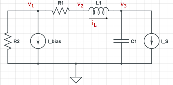
Figure 1: One tank RLC with $R1=100\mu\Omega,L1=0.5nH,C1=0.5nF$ and $R2<<R1$.

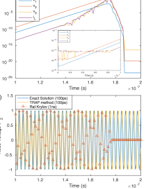
Figure 2: Simulation results of the one tank RLC (Fig. 1). (a) absolute value of $residual=C\dot{x}(t)+Gx(t)-u(t)$ for each variable in $x(t)$; (b) simulation results on $v_{3}$ with rational Krylov subspace method as well as Trapezoidal method, exact solution is included as comparison.

From the observations on ill-conditioned system from DAEs, the numerical error occurs in the calculation of algebraic variables and could result in stability issues in later simulation stage. To eliminate the error in the nullspace $\mathcal{N}({G}^{-1}{C})=\mathcal{N}({C})$, the algebraic variables are set to zero in the Arnoldi process. The technique was called implicit regularization [CCPW18].

$$v=\begin{pmatrix}v_{R}\\ v_{N}\end{pmatrix}\Rightarrow P_{C}v=\begin{pmatrix}I&0\\ 0&0\end{pmatrix}\begin{pmatrix}v_{R}\\ v_{N}\end{pmatrix}=\begin{pmatrix}v_{R}\\ 0\end{pmatrix}.$$ (114)

Since $C$ is diagonal, the matrix $P_{C}$ only contains an identity matrix for the differential variables and zeros for the algebraic variables. The approach forces the computations in the range of $C$.

Simulation results of one tank RLC with implicit regularization are shown in Fig. 3, which fit the exact solution. Residuals of $v_{3}$ and $i_{L}$ remain at a low level ($\approx 10^{-15}$) when the input current is stable. The other variable could be solved algebraically and the system no longer suffers from the singularity problem. More discussions on stability can be found in ([WCC19]).

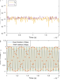
Figure 3: Simulation results of the one tank RLC (Fig. 1) with implicit regularization. (a) The absolute residual no longer increase and (b) simulation results well fit the exact solution. Node voltages $v_{1}$, $v_{2}$ are solved algebraically.

This simple example illustrates whether the numerical range of $B$ is located in the right half plane or not affects the sensitivity of numerical integration methods. Indeed, since the matrix $P_{C}G^{-1}C$ is

$$\left(\begin{array}[]{cccc}0&0&0&0\\ 0&0&0&0\\ 0&0&5\times 10^{-14}&5\times 10^{-10}\\ 0&0&-5\times 10^{-10}&0\end{array}\right),$$

${\mathcal{F}}_{C}(B)$ is the ellipse with centre $(2.5\times 10^{-14},0)$ and semi-major axis $5\times 10^{-14}$ and semi-minor axis $5\times 10^{-10}$. By (58) and Prop. 2.3, the Rayleigh quotient of the matrix $H_{m}$ always lie in the image of the ellipse under the function $g$. Thus, ${\mathcal{F}}_{C}(H_{m})$ lies in the disk ${\mathcal{D}}(1/2,1/2)$. In contrast, the ordinary Arnoldi iterations generate upper Hessenberg matrix $H_{m}$, whose numerical range ${\mathcal{F}}(H_{m})$ does not necessarily lies in ${\mathcal{D}}(1/2,1/2)$, since part of ${\mathcal{F}}(B)$ even lies in the left half plane.

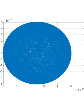
Figure 4: Illustration of ${\mathcal{F}}(G^{-1}C)$(left) and ${\mathcal{F}}_{C}(G^{-1}C)$(right) under $5\times 10^{5}$ Rayleigh quotient realizations from $\mathbb{C}^{4}$.

3.2 RLC networks

To illustrate the performance of the proposed Arnoldi algorithm on the case with $G$ only positive semi-definite, we use one PDN, consisting of $260$ resistors, $160$ capacitors and $160$ inductors. The system matrix $C$ is positive semi-define and symmetric ( actually diagonal). The matrix $G$ is positive semi-definite, but not symmetric. The eigenvalues of $B_{1,1}=V_{C}^{\top}G^{-1}CV_{C}$ are in the range of $[10^{-17},10^{-8}]$. The distribution of the eigenvalues is plotted in Fig. 5. The transient response of the RLC mesh circuit is calculated with a single step integration. Assume the slope of input current source is unchanged within the current step. Starting from zero initial state $x(0)$, the response $x(h)$ of circuit at time $h$ is derived. The exact solution is computed by directly solving differential equations and algebraic equations in (18,19).

The shift parameter $\gamma$ is set as $h/2$ empirically. The matrix exponentials in the solution are evaluated at different time step sizes $h$ with increasing dimension $m$ of Krylov subspace. For simplicity, we consider $x(0)=0=u(0)$ and the solution is given by $x(h)=h^{2}V_{C}\varphi_{2}(-hB_{1,1}^{-1})C_{1}^{-1}V_{C}^{\top}u^{\prime}(0)$. Since

$$\varphi_{0}(t)v=t^{2}\varphi_{2}(t)v+v+tv=t\varphi_{1}(t)v+v,$$

then the matrix exponential $\varphi_{2}(-hB_{1,1}^{-1})v$ appeared in the solution can be computed with a Krylov subspace approximation of either $\varphi_{0}$, $\varphi_{1}$ or $\varphi_{2}$ functions. Consider the following three approaches to compute the Krylov subspace approximation.

1. The original Arnoldi method with implicit regularization.

2. The original Arnoldi method with implicit regularization + numerical pruning of spurious eigenvalues.

3. The Arnoldi method with structured orthognality + numerical pruning of spurious eigenvalues.

Left column to right column in Fig. 6 includes the distribution of absolute error after applying approach (a), (b) and (c), respectively. Here the absolute errors are focused on matrix exponentials, thus subfigures from the top row to the bottom top shows the absolute errors of the following matrix exponentials.

1. $\varphi_{0}$ function: $V_{C}^{\top}\varphi_{0}(hB_{1,1}^{-1})V_{C}G^{-1}V_{C}^{\top}C_{1}V_{C}G^{-1}u^{\prime}(0)$.

2. $\varphi_{1}$ function: $hV_{C}^{\top}\varphi_{1}(hB_{1,1}^{-1})V_{C}G^{-1}u^{\prime}(0)$.

3. $\varphi_{2}$ function: $h^{2}V_{C}^{\top}\varphi_{1}(hB_{1,1}^{-1})C_{1}^{-1}V_{C}G^{-1}u^{\prime}(0)$.

Experiments in Fig. 6 show that the upper Hessenberg matrix can consist of many spurious eigenvalues. From (58) and (100), ${\mathcal{F}}_{C}(S)\subseteq{\mathcal{D}}(1/2,1/2)$ and thus ${\mathcal{F}}(H_{m})\subseteq{\mathcal{D}}(1/2,1/2)$. The region with spurious eigenvalues is plotted in red color. When the original Arnoldi iterations are used, the upper Hessenberg matrix could lose the positive definite property and the absolute error could grow extremely high. Clearly, the issue is resolved with (iii) see the right column. Notice that for $\gamma$ close to 0, the set ${\mathcal{F}}(H_{m})$ is very close to $1$ from(100), and rounding errors could easily contaminate the computations of $H_{m}$, such that ${\mathcal{F}}(H_{m})$ fails to lie in ${\mathcal{D}}(1/2,1/2)$. Hence, proper numerical pruning is required. Observe that the error reduces quickly with all $\varphi$ functions by increasing the dimension of rational Krylov subspace, which is consistent with the theorem 2.10. When $h$ is larger than $\mu_{2}$(the upper bound for real components of eigenvalues of $B_{1,1}$), the calculation with the $\phi_{0}$ function gives the best accuracy. On the other hand, if $h$ is smaller than the spectrum, the errors (in the log-scale) with $\varphi_{1}$ and $\varphi_{2}$ exhibit a decrease proportional to $\gamma$ in the log scale, which alleviates the error stagnation in the solution with the $\varphi_{0}$ function.

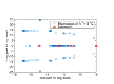
Figure 5: RLC network: eigenvalues of $B=G^{-1}C$ in log-scale.

Figure 6: RLC network with $N=507$: Left to right columns show the absolute error versus $h$ and $m$ with (a) original Arnoldi process, (b) original Arnoldi process+numerical pruning and (c) Arnoldi process with explicit structured orthogonalization +numerical pruning.

Appendix A Proofs

A.1 Proof of Theorem 1

Introduce the operator

$$\Delta_{m}:=(\lambda I-S)^{-1}-W_{m}(\lambda I-H_{m})^{-1}W_{m}^{\top}C.$$

Then the difference between (97) and (98) can be bounded by the operator on $v$,

$$\{f(S_{1,1})v-W_{m}f(H_{m})W_{m}^{\top}CV_{C}v\}$$ (115)

$$= \frac{1}{2\pi i}\int_{\Gamma}f(\lambda)\ \{(\lambda I-S)^{-1}-W_{m}(\lambda I-H_{m})^{-1}W_{m}^{\top}C\}wd\lambda$$ (116)

$$= \frac{1}{2\pi i}\int_{\Gamma}f(\lambda)\,\Delta_{m}wd\lambda.$$ (117)

By computations,

$$\Delta_{m}(\lambda I-S)W_{m}=\{W_{m}-W_{m}(\lambda I-H_{m})^{-1}W_{m}^{\top}C(\lambda I-S)W_{m}\}$$ (118)

$$= \{W_{m}-W_{m}(\lambda I-H_{m})^{-1}(\lambda I-H_{m})\}=0,$$ (119)

and thus

$$\Delta_{m}(w-(\lambda I-S)W_{m}y)=\Delta_{m}w$$ (120)

holds for any vector $y\in\mathbb{C}^{m}$. Note that columns of $W_{m}$ lie in the subspace consisting of vectors

$$\{S^{k}w:k=0,\ldots,m-1\}.$$

Hence, for each $y\in\mathbb{C}^{m}$, $w-(\lambda I-S)W_{m}y$ can be expressed as $p_{m}(S;\lambda)w$ for some polynomial $p_{m}(z;\lambda)$ of $z$ with degree $m$. Note that $p_{m}(\lambda,\lambda)=1$. Conversely, for any (degree $\leq m$) polynomial $p_{m}(z;\lambda)$ with $p_{m}(\lambda;\lambda)=1$, there exists some vector $y\in\mathbb{C}^{m}$, such that

$$w-(\lambda I-S)W_{m}y=p_{m}(S;\lambda).$$

All together, for any $\lambda\in\Gamma$, from (117) and (120), we have

$$V_{C}f(S_{1,1})v-W_{m}f(H_{m})W_{m}^{\top}CV_{C}v=\frac{1}{2\pi i}\int_{\Gamma}f(\lambda)\Delta_{m}p_{m}(S;\lambda)w\,d\lambda.$$

Choose $\Gamma$ to be the circle with centre $c_{0}$ and radius $r$ and

$$p_{m}(z;\lambda)=(\frac{z-c_{0}}{r})^{m}.$$

We have

$$V_{C}f(S_{1,1})v-V_{C}V_{C}^{\top}W_{m}f(H_{m})W_{m}^{\top}CV_{C}v=\frac{1}{2\pi i}\int_{\Gamma}f(\lambda)\Delta_{m}\left(\frac{S-c_{0}I}{r}\right)^{m}wd\lambda$$ (121)

$$= \frac{(\rho_{0}/r)^{m}}{2\pi i}\int_{\Gamma}f(\lambda)\Delta_{m}\left(\frac{S-c_{0}I}{\rho_{0}}\right)^{m}wd\lambda.$$ (122)

By Prop. 2.3, ${\mathcal{F}}_{C}(S)$ is bounded by a disk ${\mathcal{D}}(c_{0},\rho_{0})$. Then Prop. 2.5 and the power inequality in theorem in ([Pea66]) indicate

$$|{\mathcal{F}}_{C}(\rho_{0}^{-1}(S-c_{0}I))|\leq 1,\;|{\mathcal{F}}_{C}((\rho_{0}^{-1}(S-c_{0}I))^{m})|\leq 1,$$

and thus

$$\|(\rho_{0}^{-1}(S-c_{0}I))^{m}u\|_{C}\leq 2\|u\|_{C}.$$

Hence, with the aid of Prop. 2.6 and (58),

$$\|(\lambda I-S)^{-1}\|_{C}\leq d(\Gamma,{\mathcal{F}}_{C}(S))^{-1},\|W_{m}(\lambda I-H)^{-1}W_{m}^{\top}C\|_{C}\leq\|(\lambda I-H)^{-1}\|\leq d(\Gamma,{\mathcal{F}}_{C}(S))^{-1},$$

and then

$$\|\Delta_{m}w\|_{C}\leq 2d(\Gamma,{\mathcal{F}}_{C}(S))^{-1}\|w\|_{C},$$

where $d(\Gamma,{\mathcal{F}}_{C}(S))$ is the shortest distance between $\Gamma$ and ${\mathcal{F}}_{C}(S)$. From (120),

$$\|\Delta_{m}w\|_{C}=\|\Delta_{m}p_{m}(S;\lambda)w\|_{C}\leq 2d(\Gamma,{\mathcal{F}}_{C}(S))^{-1}\cdot\|p_{m}(S;\lambda)w\|_{C}\leq\frac{2}{r-\rho_{0}}\cdot 2\left(\frac{\rho_{0}}{r}\right)^{m}\|w\|_{C},$$

We have for unit vector $v$

$$\|V_{C}f(S_{1,1})v-W_{m}f(H_{m})W_{m}^{\top}CV_{C}v\|_{C}\leq(\max_{\lambda\in\Gamma}|f(\lambda)|)\cdot 2d(\Gamma,{\mathcal{F}}_{C}(S))^{-1}\cdot\|p_{m}(S;\lambda)w\|_{C}$$ (123)

$$\leq (\max_{\lambda\in\Gamma}|f(\lambda)|)\cdot\frac{4}{r-\rho_{0}}(\frac{\rho_{0}}{r})^{m}.$$ (124)

From (36), (30) and (43), the quality of $x_{a}$ in (43) can be analyzed in the following inequality,

$$\|x_{\mathcal{R}}(t)-x_{a}(t)\|_{C}\leq\|\{V_{C}f(S_{1,1})V_{C}^{\top}-W_{m}^{(0)}f(H_{m}^{(0)}){W_{m}^{(0)}}^{\top}C\}x(0)\|_{C}$$ (125)

$$+ \|\{V_{C}f_{1}(S_{1,1})V_{C}^{\top}-W_{m}^{(1)}f_{1}(H_{m}^{(1)}){W_{m}^{(1)}}^{\top}C\}u(0)\|_{C}$$ (126)

$$+ \|\{V_{C}f_{2}(S_{1,1})V_{C}^{\top}-W_{m}^{(2)}f_{2}(H_{m}^{(2)}){W_{m}^{(2)}}^{\top}C\}u^{\prime}(0)\|_{C},$$ (127)

which completes the proof.

A.2 Proof of Prop. 2.11

Proof.

Derivatives of $\rho,c_{0}$ with respect to $\gamma$ are

$$\frac{dc_{0}}{d\gamma}=-\frac{1}{2}\left(\frac{\mu_{2}}{(\gamma+\mu_{2})^{2}}+\frac{\mu_{1}}{(\gamma+\mu_{1})^{2}}\right)<0$$ (128)

and

$$\frac{d\rho}{d\gamma}=\frac{1}{2}\{-\frac{\mu_{2}}{(\mu_{2}+\gamma)^{2}}+\frac{\mu_{1}}{(\mu_{1}+\gamma)^{2}}\}.$$ (129)

Then

$$\frac{d}{d\gamma}(\log\rho-\log c_{0})=\frac{1}{\rho}\frac{d\rho}{d\gamma}-\frac{1}{c_{0}}\frac{dc_{0}}{d\gamma}$$ (130)

$$= -\left(\frac{\frac{\mu_{2}}{(\gamma+\mu_{2})^{2}}-\frac{\mu_{1}}{(\gamma+\mu_{1})^{2}}}{\frac{\mu_{2}}{(\gamma+\mu_{2})}-\frac{\mu_{1}}{(\gamma+\mu_{1})}}\right)+\left(\frac{\frac{\mu_{2}}{(\gamma+\mu_{2})^{2}}+\frac{\mu_{1}}{(\gamma+\mu_{1})^{2}}}{\frac{\mu_{2}}{(\gamma+\mu_{2})}+\frac{\mu_{1}}{(\gamma+\mu_{1})}}\right)$$ (131)

$$= 2\left(\frac{\frac{\mu_{2}}{(\gamma+\mu_{2})^{2}}\frac{\mu_{1}}{(\gamma+\mu_{1})^{2}}(\gamma+\mu_{2}-\gamma-\mu_{1})}{(\frac{\mu_{2}}{(\gamma+\mu_{2})})^{2}-(\frac{\mu_{1}}{(\gamma+\mu_{1})})^{2}}\right)$$ (132)

$$= 2((\mu_{1}^{-1}+\mu_{2}^{-1})\gamma^{2}+2\gamma)^{-1}>0.$$ (133)

∎

A.3 Proof of Prop. 2.12

Proof.

By computations,

$$\frac{d}{d\gamma}\log E(\gamma)=\frac{d}{d\gamma}\{\delta(1-\frac{1}{2c_{0}})+m\log\frac{\rho}{c_{0}}-\log(c-\rho)\}$$ (134)

$$= -\delta(\frac{1}{4c_{0}^{2}}(\frac{\mu_{2}}{(\gamma+\mu_{2})^{2}}+\frac{\mu_{1}}{(\gamma+\mu_{1})^{2}}))+2m((\frac{1}{\mu_{1}}+\frac{1}{\mu_{2}})\gamma^{2}+2\gamma)^{-1}+(\mu_{1}+\gamma)^{-1}$$ (135)

$$= -\delta\frac{\mu_{2}(\gamma+\mu_{1})^{2}+\mu_{1}(\gamma+\mu_{2})^{2}}{(2\mu_{1}\mu_{2}+\gamma(\mu_{1}+\mu_{2}))^{2}}+\frac{m}{\gamma}(\frac{2\mu_{1}\mu_{2}}{(\mu_{1}+\mu_{2})\gamma+2\mu_{1}\mu_{2}})+(\mu_{1}+\gamma)^{-1}$$ (136)

$$= \xi^{-1}\{-\delta+\frac{m}{\gamma}(\frac{2\mu_{1}\mu_{2}}{(\mu_{1}+\mu_{2})\gamma+2\mu_{1}\mu_{2}})\xi+(\mu_{1}+\gamma)^{-1}\xi\}.$$ (137)

Here the function $\xi(\gamma)$ introduced has an upper bound decreasing with respect to $\gamma$,

$$\xi(\gamma):=\frac{\mu_{1}^{2}(\mu_{2}+\gamma)^{2}}{\mu_{1}(\mu_{2}+\gamma)^{2}}\frac{(1+\frac{\mu_{2}(\mu_{1}+\gamma)}{\mu_{1}(\mu_{2}+\gamma)})^{2}}{1+\frac{\mu_{2}(\mu_{1}+\gamma)^{2}}{\mu_{1}(\mu_{2}+\gamma)^{2}}}=\mu_{1}\frac{1+2\frac{\mu_{2}(\mu_{1}+\gamma)}{\mu_{1}(\mu_{2}+\gamma)}+(\frac{\mu_{2}(\mu_{1}+\gamma)}{\mu_{1}(\mu_{2}+\gamma)})^{2}}{1+\frac{\mu_{2}(\mu_{1}+\gamma)^{2}}{\mu_{1}(\mu_{2}+\gamma)^{2}}}$$ (138)

$$\leq \mu_{1}(1+2(\frac{\mu_{2}+\gamma}{\mu_{1}+\gamma})+\frac{\mu_{2}}{\mu_{1}})=\mu_{1}+\mu_{2}+2\frac{\mu_{1}}{\mu_{1}+\gamma}(1+\mu_{2}-\mu_{1}).$$ (139)

Using the AM-GM inequality on the denominator for the second term of (138), we have one upper bound for $\xi$,

$$\xi(\gamma)\leq\mu_{1}(1+\sqrt{2\mu_{2}/\mu_{1}}+\mu_{2}/\mu_{1})=(\sqrt{\mu_{1}}+\sqrt{\mu_{2}})^{2}.$$

Hence, for $\gamma\geq\mu_{2}$, (137) gives

$$-\frac{d}{d\gamma}\log E(\gamma)\geq(\sqrt{\mu_{1}}+\sqrt{\mu_{2}})^{-2}\left\{\delta-\{\frac{2m\mu_{1}}{\mu_{2}(3\mu_{1}+\mu_{2})}+\frac{1}{\mu_{2}+\mu_{1}}\}(\sqrt{\mu_{1}}+\sqrt{\mu_{2}})^{2}\right\}.$$

∎

References

- [BGH13] Mike A. Botchev, Volker. Grimm, and Marlis. Hochbruck. Residual, restarting, and richardson iteration for the matrix exponential. SIAM Journal on Scientific Computing, 35(3):A1376–A1397, 2013.
- [BR09] BERNHARD BECKERMANN and LOTHAR REICHEL. Error estimates and evaluation of matrix functions via the faber transform. SIAM Journal on Numerical Analysis, 47(5):3849–3883, 2009.
- [BS67] C. A. Berger and J. G. Stampfli. Mapping theorems for the numerical range. American Journal of Mathematics, 89(4):1047–1055, 1967.
- [CCPW18] Pengwen Chen, Chung Kuan Cheng, Dongwon Park, and Xinyuan Wang. Transient circuit simulation for differential algebraic systems using matrix exponential. In Proceedings of the International Conference on Computer-Aided Design, page 99. ACM, 2018.
- [CMV69] W.J Cody, G Meinardus, and R.S Varga. Chebyshev rational approximations to e−x in [0, +∞) and applications to heat-conduction problems. Journal of Approximation Theory, 2(1):50 – 65, 1969.
- [Cro07] Michel Crouzeix. Numerical range and functional calculus in hilbert space. Journal of Functional Analysis, 244(2):668 – 690, 2007.
- [DK98] Vladimir Druskin and Leonid Knizhnerman. Extended krylov subspaces: Approximation of the matrix square root and related functions. SIAM Journal on Matrix Analysis and Applications, 19(3):755–771, 1998.
- [ER80] Thomas Ericsson and Axel Ruhe. The spectral transformation lanczos method for the numerical solution of large sparse generalized symmetric eigenvalue problems. Mathematics of Computation, 35(152):1251–1268, 1980.
- [Eri86] Thomas Ericsson. A generalised eigenvalue problem and the lanczos algorithm. In Jane Cullum and Ralph A. Willoughby, editors, Large Scale Eigenvalue Problems, volume 127 of North-Holland Mathematics Studies, pages 95 – 119. North-Holland, 1986.
- [Fre00] Roland W Freund. Krylov-subspace methods for reduced-order modeling in circuit simulation. Journal of Computational and Applied Mathematics, 123(1-2):395–421, 2000.
- [FTDR89] Richard A. Friesner, Laurette S. Tuckerman, Bright C. Dornblaser, and Thomas V. Russo. A method for exponential propagation of large systems of stiff nonlinear differential equations. Journal of Scientific Computing, 4(4):327–354, 1989.
- [GG17] Volker Grimm and Tanja Göckler. Automatic smoothness detection of the resolvent krylov subspace method for the approximation of $c_0$-semigroups. SIAM Journal on Numerical Analysis, 55(3):1483–1504, 2017.
- [GH08] V. Grimm and M. Hochbruck. Rational approximation to trigonometric operators. BIT Numerical Mathematics, 48(2):215–229, 2008.
- [Göc14] Tanja Göckler. Rational Krylov subspace methods for phi-functions in exponential integrators. PhD thesis, 2014.
- [Gri12] Volker Grimm. Resolvent krylov subspace approximation to operator functions. BIT Numerical Mathematics, 52(3):639–659, 2012.
- [Hig08] Nicholas J. Higham. Functions of Matrices. Society for Industrial and Applied Mathematics, 2008.
- [HL97] Marlis. Hochbruck and Christian. Lubich. On Krylov subspace approximations to the matrix exponential operator. SIAM Journal on Numerical Analysis, 34(5):1911–1925, 1997.
- [HO10] Marlis Hochbruck and Alexander Ostermann. Exponential integrators. Acta Numerica, 19:209–286, 2010.
- [HOS09] Marlis Hochbruck, Alexander Ostermann, and Julia Schweitzer. Exponential rosenbrock-type methods. SIAM Journal on Numerical Analysis, 47(1):786–803, 2009.
- [IR14] Achim Ilchmann and Timo Reis. Surveys in differential-algebraic equations II. Springer, 2014.
- [JdlCM20] J.C. Jimenez, H. [de la Cruz], and P.A. [De Maio]. Efficient computation of phi-functions in exponential integrators. Journal of Computational and Applied Mathematics, 374:112758, 2020.
- [Joh78] Charles R. Johnson. Numerical determination of the field of values of a general complex matrix. SIAM Journal on Numerical Analysis, 15(3):595–602, 1978.
- [MKEW96] L. Miguel Silveira, M. Kamon, I. Elfadel, and J. White. A coordinate-transformed arnoldi algorithm for generating guaranteed stable reduced-order models of rlc circuits. In Proceedings of International Conference on Computer Aided Design, pages 288–294, Nov 1996.
- [MS97] Karl Meerbergen and Alastair Spence. Implicitly restarted arnoldi with purification for the shift-invert transformation. Math. Comput., 66(218):667–689, April 1997.
- [MVL78] Cleve Moler and Charles Van Loan. Nineteen dubious ways to compute the exponential of a matrix. SIAM Review, 20(4):801–836, 1978.
- [MVL03] C. Moler and C. Van Loan. Nineteen dubious ways to compute the exponential of a matrix, twenty-five years later. SIAM review, 45(1):3–49, 2003.
- [Nas08] Sani R Nassif. Power grid analysis benchmarks. In Design Automation Conference, 2008. ASPDAC 2008. Asia and South Pacific, pages 376–381. IEEE, 2008.
- [NOPEJ87] Bahram Nour-Omid, Beresford N Parlett, Thomas Ericsson, and Paul S Jensen. How to implement the spectral transformation. Mathematics of Computation, 48(178):663–673, 1987.
- [NW12] Jitse Nissen and Will M. Wright. a krylov subspace algorithm for evaluating the phi function appearing in exponential integrators. ACM Transactions on Mathematical Software, 38(3):1–21, 2012.
- [Pea66] Carl Pearcy. An elementary proof of the power inequality for the numerical radius. Michigan Math. J., 13(3):289–291, 1966.
- [RM09] Joost Rommes and Nelson Martins. Exploiting structure in large-scale electrical circuit and power system problems. Linear Algebra and its Applications, 431(3-4):318–333, 2009.
- [Ruh84] Axel Ruhe. Rational krylov sequence methods for eigenvalue computation. Linear Algebra and its Applications, 58:391 – 405, 1984.
- [Saa92] Yousef Saad. Analysis of some krylov subspace approximations to the matrix exponential operator. SIAM J. Numer. Anal., 29(1):209–228, 1992.
- [SFR93] B. Simeon, C. Führer, and P. Rentrop. The drazin inverse in multibody system dynamics. Numerische Mathematik, 64(1):521–539, 1993.
- [TI10] Mizuyo Takamatsu and Satoru Iwata. Index characterization of differential–algebraic equations in hybrid analysis for circuit simulation. International Journal of Circuit Theory and Applications, 38(4):419–440, 2010.
- [Tre12] Lloyd N. Trefethen. Approximation Theory and Approximation Practice (Other Titles in Applied Mathematics). Society for Industrial and Applied Mathematics, USA, 2012.
- [Wan06] Gerhard Wanner. Dahlquist’s classical papers on stability theory. BIT Numerical Mathematics, 46(3):671–683, 2006.
- [WCC12] Shih-Hung Weng, Quan Chen, and Chung Kuan Cheng. Time-domain analysis of large-scale circuits by matrix exponential method with adaptive control. IEEE TCAD, 31(8):1180–1193, 2012.
- [WCC19] X. Wang, P. Chen, and C. Cheng. Stability and convergency exploration of matrix exponential integration on power delivery network transient simulation. IEEE Transactions on Computer-Aided Design of Integrated Circuits and Systems, pages 1–1, 2019.
- [Win03] Renate Winkler. Stochastic differential algebraic equations of index 1 and applications in circuit simulation. Journal of computational and applied mathematics, 157(2):477–505, 2003.
- [ZYW+16] Hao Zhuang, Wenjian Yu, Shih-Hung Weng, Ilgweon Kang, Jeng-Hau Lin, Xiang Zhang, Ryan Coutts, and Chung Kuan Cheng. Simulation algorithms with exponential integration for time-domain analysis of large-scale power delivery networks. IEEE TCAD, 35(10):1681–1694, 2016.