Machine Learning for Observables: Reactant to Product State Distributions for Atom-Diatom Collisions

Abstract

Machine learning-based models to predict product state distributions from a distribution of reactant conditions for atom-diatom collisions are presented and quantitatively tested. The models are based on function-, kernel- and grid-based representations of the reactant and product state distributions. While all three methods predict final state distributions from explicit quasi-classical trajectory simulations with $R^{2}>0.998$, the grid-based approach performs best. Although a function-based approach is found to be more than two times better in computational performance, the kernel- and grid-based approaches are preferred in terms of prediction accuracy, practicability and generality. The function-based approach also suffers from lacking a general set of model functions. Applications of the grid-based approach to non-equilibrium, multi-temperature initial state distributions are presented, a situation common to energy distributions in hypersonic flows. The role of such models in Direct Simulation Monte Carlo and computational fluid dynamics simulations is also discussed.

I Introduction

The realistic description of chemical and reactive systems with a large number of available states, such as explosions, hypersonic gas flow around space vehicles upon re-entry into the atmosphere, or meteorites penetrating deep into the lower parts of Earth’s or a planet’s atmosphere, requires an understanding of the relevant processes at a molecular level.Park (1993); Bertin and Cummings (2003); Koner, Bemish, and Meuwly (2020) Correctly describing the population of the available state space under such non-equilibrium conditions (e.g. high temperatures in atmospheric re-entry with $T>10000$ K) from ground-based experiments is extremely challenging. Such high gas temperatures make the gathering of experimental data exceedingly difficult but is essential for simulations of hypersonic flight.Boyd (2015) On the other hand, a comprehensive modeling of gas phase chemical reactions through explicit molecular-level simulations remains computationally challenging due to the large number of accessible states and transitions between them.Grover, Torres, and Schwartzentruber (2019); Koner et al. (2019) There are also other, similar situations in physical chemistry such as the spectroscopy in hot environments (e.g. on the sun) for which small polyatomic molecules can populate a large number of rovibrational statesRothman et al. (2005) between which transitions can take place. Exhaustively probing and enumerating all allowed transitions or creating high-dimensional analytical representations for them is usually not possible. Nevertheless, it is essential to have complete line lists available because, if specific states that are involved in important transitions are omitted, modeling of the spectroscopic bands becomes difficult or even impossible.Yurchenko et al. (2014) This points towards an important requirement for such models, namely that they contain the majority of the important information while remaining sufficiently fast to evaluate.

In such situations, machine learning approaches can provide an alternative to address the problem of characterizing product distributions from given reactant state distributions. In previous workKoner et al. (2019), a model for state-to-state (STS) cross sections of an atom-diatom collision system using a neural network (NN) has been proposed. Motivated by the success of such an approach, the present work attempts to develop a NN-based distribution-to-distribution (DTD) model for the relative translational energy $E_{\rm trans}$, the vibrational $v$ and rotational $j$ states of a reactive atom-diatom collision system. In other words, given the reactant state distributions ($P(E_{\text{trans}}),P(v),P(j)$) such a model predicts the three corresponding product state distributions ($P(E_{\text{trans}}^{\prime}),P(v^{\prime}),P(j^{\prime})$). Here, $P(v)$ and $P(j)$ are marginal distributions, i.e. $P(v)=\sum_{j}P(v,j)$ and $P(j)=\sum_{v}P(v,j)$, where $(v,j)$ labels the rovibrational state of the diatom.Singh and Schwartzentruber (2018) Hence, instead of considering all possible combinations of ($E_{\text{trans}},v,j$) on the reactant (input) and product (output) side explicitly, one is rather interested in a description of these microscopic quantities by means of their underlying probability distributions.

While the state-to-state specificity is lost, such a probabilistic approach considerably reduces the computational complexity of the problem at hand. While a STS-approach is still feasible for an atom-diatom collision system with $\sim 10^{7}$ STS cross sectionsKoner et al. (2019), it becomes intractableSchwartzentruber, Grover, and Valentini (2018) even for a diatom-diatom type collision system due to the dramatic increase in the number of STS cross sections to $\sim 10^{15}$. Moreover, such DTD models still allow for the prediction of quantities relevant to hypersonic flow, such as the reaction rates or the average vibrational and rotational energies.Singh and Schwartzentruber (2020a)

Here, the N + O${}_{2}\rightarrow$ NO + O reaction is considered, which is relevant in the hypersonic flight regime and for which accurate, fully dimensional potential energy surfaces (PESs) are available.San Vicente Veliz et al. (2020) The necessary reference data to train the NN-based models was obtained by running explicit quasi-classical trajectories (QCT) for reactive N + O₂ collisions. In particular, from a diverse set of equilibrium reactant state distributions ($P(E_{\text{trans}}),P(v),P(j)$) for N + O₂, the corresponding product distributions for NO + O are obtained by means of QCT simulations. In this work, three different approaches for learning and characterizing these distributions are pursued, including function-, kernel-, and grid-based models (F-, K-, and G-based models in the following). The microscopic description provided by such DTD models can, e.g., be used as an input or to develop models for more coarse-grained approaches, including Direct Simulation Monte CarloBird (1994) (DSMC) or computational fluid dynamics (CFD) simulations. Furthermore, the core findings of this work also carry over to applications in other areas where a DTD model is of interest, such as in demographicsFlaxman et al. (2016) or economicsPerotti (1996).

This work is structured as follows. First, the methods including three different approaches to construct NN-based DTD models are described. Then, the performance of the models is assessed for various data sets and improvements in particular related to the input features are explored. Finally, implications for modeling hypersonic gas flow, based on DSMC and CFD simulations, are discussed and conclusions are drawn.

II Methods

II.1 Quasi-Classical Trajectory Calculations

Explicit QCT simulations for the N + O₂ collision system were carried out on the ⁴A^′ PES of NO₂ following previous work.Truhlar and Muckerman (1979); Henriksen and Hansen (2011); Koner et al. (2016); Koner, Bemish, and Meuwly (2018); San Vicente Veliz et al. (2020) Specifically, the reactive channel for the N + O₂ $\rightarrow$ NO + O collision was considered. The ⁴A^′ PES is chosen here, because this state contributes most to the equilibrium rate.San Vicente Veliz et al. (2020) Briefly, Hamilton’s equations of motion are solved in reactant Jacobi coordinates using a fourth-order Runge-Kutta method with a time step of $\Delta t=0.05$ fs, which guarantees conservation of the total energy and angular momentum. The initial conditions for each trajectory were randomly chosen using standard Monte Carlo sampling methods.Truhlar and Muckerman (1979); Henriksen and Hansen (2011) The initial relative translational energies $E_{\rm trans}$ were sampled from Maxwell-Boltzmann distributions ($E_{\rm trans,min}=0.0$ eV; $E_{\rm trans,max}=19.8$ eV;$\Delta E_{\rm trans}=0.1$ eV) and reactant vibrational $v$ and rotational $j$ states were sampled from Boltzmann distributions ($v_{\rm min}=0,v_{\rm max}=38,\Delta v=1$; $j_{\rm min}=0,j_{\rm max}=242,\Delta j=1$), characterized by $T_{\text{trans}}$, $T_{\text{vib}}$ and $T_{\text{rot}}$, respectively.Truhlar and Muckerman (1979); Bender et al. (2015) The impact parameter $b$ was sampled from 0 to $b_{\rm max}=10$ Å using stratified samplingTruhlar and Muckerman (1979); Bender et al. (2015) with 6 equidistant strata. The rovibrational reactant (O₂; $(v,j)$) and product diatom (NO; $(v^{\prime},j^{\prime})$) states are calculated following semiclassical theory of bound states.Karplus, Porter, and Sharma (1965) The states of the product diatom are assigned using histogram binning.

First, models were constructed for the case $T_{\text{rovib}}=T_{\text{rot}}=T_{\text{vib}}$, for which QCT simulations were performed at $T_{\text{trans}}$ and $T_{\text{rovib}}$ ranging from 5000 K to 20000 K in increments of 250 K. This yielded 3698 sets of reactant state distributions and corresponding product state distributions which will be referred to as “Set1”. Next, for the more general case $T_{\text{rot}}\neq T_{\text{vib}}$, further QCT simulations were performed for $T_{\text{trans}}=5000,10000,15000,20000$ K with $T_{\text{vib}}$ and $T_{\text{rot}}$ each ranging from 5000 K to 20000 K in increments of 1000 K. This gives an additional 960 data sets and a total of 4658 data sets that include both cases, $T_{\text{rot}}=T_{\text{vib}}$ and $T_{\text{rot}}\neq T_{\text{vib}}$, collectively referred to as “Set2”.

The reactant and product state distributions of Set1 and Set2 constitute representative reference data to train and validate NN-based models. For both sets the temperatures $\bm{T}=(T_{\text{trans}}$, $T_{\text{vib}}$, $T_{\text{rot}}$) completely specify the reactant and product state distributions as they are related through the explicit QCT simulations. Hence, for brevity a specific set of reactant and product state distributions is referred to as $\bm{T}$.

II.2 Generating Nonequilibrium Data Sets

In hypersonic applications it is known that quantities such as $P(E_{\text{trans}})$, $P(v)$, or $P(j)$ are typically nonequilibrium probability distributions.Boyd (2015) This has also been confirmed in explicit simulation studies, starting from equilibrium energy and state distributions as is commonly done in QCT simulations.Denis-Alpizar, Bemish, and Meuwly (2017); Koner, Bemish, and Meuwly (2018) Therefore, a general DTD model should be able to correctly predict (nonequilibrium) product state distributions starting from nonequilibrium reactant state distributions. With this in mind, and with Set2 at hand, new reactant and product state distributions were generated by means of a weighted sum of the existing distributions according to

$$P(i)=\frac{1}{w_{\text{tot}}}\sum_{n=1}^{N}w_{n}\cdot P_{n}(i).$$ (1)

Here, $i\in[E_{\text{trans}},v,j,E_{\text{trans}}^{\prime},v^{\prime},j^{\prime}]$ labels the degree of freedom, $n$ labels the data set, $N\in[2,3]$ is the total number of distributions drawn from Set2, the corresponding distributions $P_{n}(i)$ used for and obtained from QCT simulations and the random weights $w_{n}\in[1,2]$ determine how much these contribute to the total sum. The resulting distributions are scaled by $w_{\text{tot}}=\sum_{n=1}^{N}w_{n}$ to conserve probability. Such distributions then constitute Set3. It is assumed that any nonequilibrium state distribution can be represented as a decomposition in terms of a linear combination of equilibrium distributions given by Eq. 1. For instance, general nonequilibrium distributions for nitrogen and oxygen relaxation at high temperature ($>8000$ K) conditions, obtained via direct molecular simulations (DMS), which is equivalent to solving the full master equation, have been successfully modelled as a weighted sum of two Boltzmann distributions.Singh and Schwartzentruber (2020b) Consequently, DTD models that are successfully trained and validated on Set3 are also expected to generalize well to most nonequilibrium situations encountered in practice.

In the following, a single data set for Set3 is generated by randomly specifying the number of distributions $N\in[2,3]$ to be combined although larger values for $N$ are possible and will be explored later. The final set of reactant and product state distributions is characterized by $N$ sets of temperatures $\bm{T}$ and corresponding normalized weights $\bm{w}=(w_{1}/w_{\rm tot},...,w_{N}/w_{\rm tot})$. The product state distributions obtained by this procedure are akin to explicit QCT simulations using Monte Carlo sampling of the reactant state distributions by sampling each of the equilibrium distributions in the corresponding weighted sum. In the following, three different possibilities for characterizing reactant and product state distributions are described.

II.3 Function (F)-Based Approach

In the F-based approach, each set of relative translational energy, vibrational and rotational state distributions of reactant and product are fitted to parametrized model functions, see Figure 1 for an example. The corresponding fitting parameters in Eqs. 2 to 7 constitute the input and output of a NN, respectively (see Section II.6 for details on the NN). Together with the parametrized model functions (Eqs. 2 to 7) this serves as a map between reactant and product state distributions, i.e., a DTD model. In this work the F-based approach was only applied to Set1.

The set of model functions used here was

$$\tilde{P}(E_{\text{trans}})=a_{1}E_{\text{trans}}\cdot\exp(-E_{\text{trans}}/a_{2}),$$ (2)

$$\tilde{P}(v)=b_{1}\exp(-v/b_{2}),$$ (3)

$$\tilde{P}(j)=c_{1}\exp(-j/c_{2})+c_{3}\exp(-(\ln(2c_{4}(j-c_{5})/c_{6}+1)/c_{4})^{2}),$$ (4)

$$\tilde{P}(E_{\text{trans}}^{\prime})=d_{1}\exp(-(\ln(2d_{2}(E_{\text{trans}}^{\prime}-d_{3})/d_{4}+1)/d_{2})^{2}),$$ (5)

$$\tilde{P}(v^{\prime})=e_{1}v^{\prime 4}+e_{2}v^{\prime 3}+e_{3}v^{\prime 2}+e_{4}v^{\prime}+e_{5},$$ (6)

$$\tilde{P}(j^{\prime})=f_{1}\exp(-j^{\prime}/f_{2})+f_{3}\exp(-(\ln(2f_{4}(j^{\prime}-f_{5})/f_{6}+1)/f_{4})^{2}),$$ (7)

where $\bm{a}=(a_{1},a_{2})$ through $\bm{f}=(f_{1},...,f_{6})$ are the fitting parameters of the model functions. In total, this results in 10 and 15 fitting parameters for one set of reactant or product state distribution, respectively. For the reactant and product rotational state distributions, $P(j)$ and $P(j^{\prime})$, the same model function was used. Such a parametric approach has its foundation in surprisal analysisLevine (1978) which was recently used in models for hypersonics.Singh and Schwartzentruber (2018, 2020c, 2020a)

The reactant state distributions in Set1 are equilibrium distributions and the model functions (Eqs. 2 to 4) were chosen accordingly. For the product state distributions, which are typically nonequilibrium distributions, modified parametrizations were used after inspection of the results from the QCT simulations. Here, it is worth mentioning that using alternative parametrizations for model functions are possible, too, which will be briefly explored later.

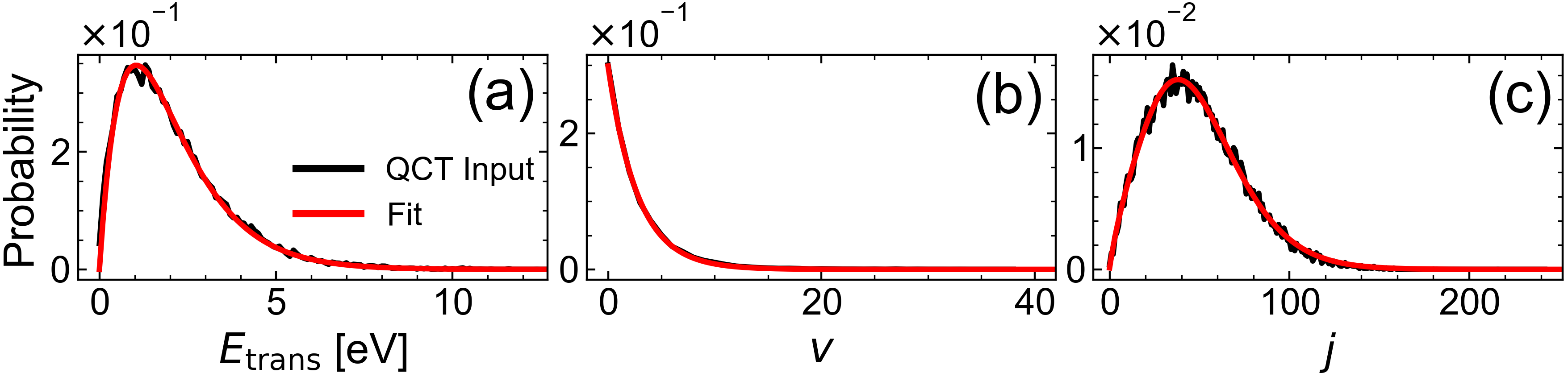
Figure 1: Reactant state distributions for the F-based approach: $P(E_{\rm trans})$ ($T_{\text{trans}}=12500$ K, panel (a), $P(v)$ (panel (b)) and $P(j)$ (panel (c)) distributions ($T_{\text{rovib}}=5750$ K) for explicit QCT simulations (black) and corresponding fits (red) obtained using Eqs. 2 to 4.

II.4 Kernel (K)-Based Approach

The representer theoremSchölkopf, Herbrich, and Smola (2001) states that, given $N$ grid points $x_{i}$, the function $f(x)$ can always be approximated as a linear combination of suitable functions

$$f(x)\approx\widetilde{f}(x)=\sum_{i=1}^{N}c_{i}K(x,x_{i})$$ (8)

where $c_{i}$ are coefficients and $K(x,x_{i})$ is a kernel function. The reproducing property asserts that $f(x^{\prime})=\langle f(x),K(x,x^{\prime})\rangle$ where $\langle\cdot\rangle$ is the scalar product, $K(x,x^{\prime})$ is the kernelAronszajn (1950) and the coefficients $c_{i}$ are determined through matrix inversion. This leads to a reproducing kernel Hilbert space (RKHS) representation that exactly reproduces the function at the grid points $x_{i}$.Aronszajn (1950); Ho and Rabitz (1996); Unke and Meuwly (2017) In the present work the amplitudes of the distributions at the chosen grid points are used for inter- and extrapolation based on a RKHS-based representation and the the coefficients $c_{i}$ serve as input and output of the NN. Hence, given the kernel coefficients for the reactant state distributions, the NN is trained to predict the coefficients of the corresponding product state distributions. Together with the associated grids, one obtains a continuous (K+NN-based) prediction of the product state distributions, i.e., a DTD model. The K-based approach was also only applied to Set1.

In this work, a Gaussian kernel

$$K(x,x^{\prime})=\exp(-|x-x^{\prime}|^{2}/2\sigma^{2}),$$ (9)

with hyperparameter $\sigma$ was found to perform well as a reproducing kernel. Furthermore, a variable amount of regularization as specified by the regularization rate $\lambda$ in the Tikhonov-scheme is used. The hyperparameters $\sigma$ and $\lambda$ remain to be optimized systematically. However, the present choices yielded sufficiently accurate representations. Assigning $\sigma$ to the average spacing between neighbouring grid points was found to be advantageous. Alternatively, it is also possible to choose $\sigma$ at each grid point to be equal to the larger of the two neighbouring grid spacings. In this work, the first approach is used for $P(v)$ and $P(v^{\prime})$, whereas the second approach is applied for all other distributions. Moreover, such choices for $\sigma$ significantly reduced the number of grid points required for accurate RKHS approximations and the resulting kernel coefficients lead to accurate NN predictions. While the same level of accuracy for the RKHS approximations can be achieved with larger values for $\sigma$, the accuracy of the resulting NN predictions was found to deteriorate. Consequently, only the regularization rate $\lambda$ needed to be tuned and accurate RKHS approximations were obtained after a few iterations.

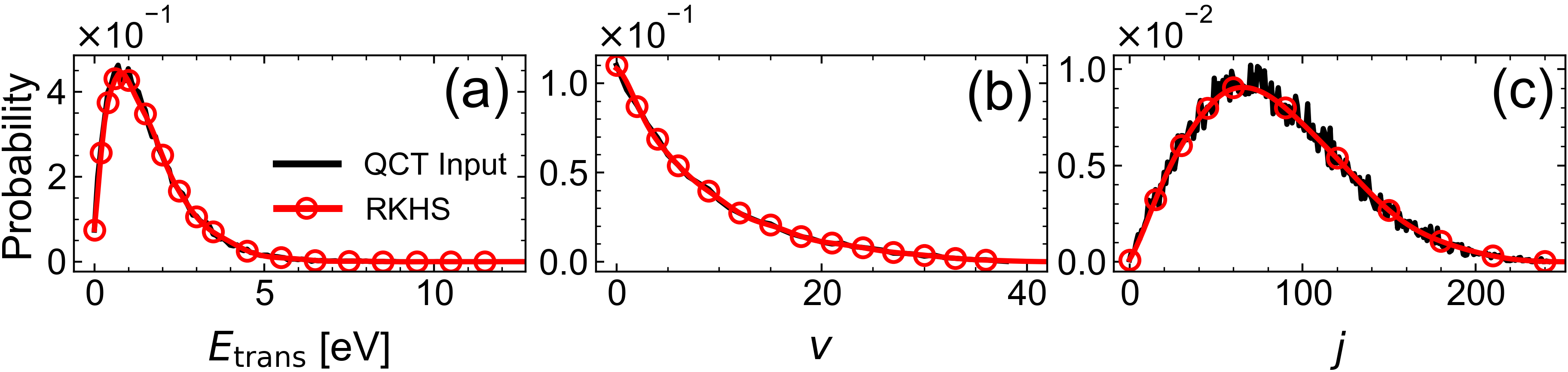
Figure 2: Reactant state distributions for K- and G-based approaches: $P(E_{\rm trans})$ ($T_{\text{trans}}=9500$ K, panel (a), $P(v)$ (panel (b)) and $P(j)$ (panel (c)) distributions ($T_{\text{rovib}}=16000$ K) for explicit QCT simulations (black), their RKHS representations (red lines) and the locally averaged values at the corresponding grid points (red circles) used for the G-based approach.

The location and number of grid points for the reactant and product state distributions is largely arbitrary but should be governed by the overall shape of the distributions, see Figure 2 for an example. The grids used here are reported in Table S1. The number of grid points for reactant and product state distributions differs because they are equilibrium and nonequilibrium distributions, respectively. Also, depending on the shape of the distributions to be represented, additional points may be required to avoid unphysical undulations in the RKHS approximations. For the system considered here, this is mainly observed for $P(v^{\prime})$ which requires a denser grid than the corresponding reactant state distributions $P(v)$.

Instead of directly evaluating the distributions at the grid points, local averaging over neighboring data points according to

$$\bar{P}(x_{i})=\frac{1}{2n+1}\sum\limits_{j=i-n}^{i+n}P(x_{j}),$$ (10)

was performed to obtain $\bar{P}(x_{i})$. Here $n={\rm min}(n_{\rm max},n_{\rm nb})$, with $n_{\rm nb}$ the maximum number of neighbouring data points to the left or the right. If the first and last data points are chosen as grid points they were assigned the unaveraged distribution values. The value of $n_{\text{max}}$ can differ for each of the ($E_{\text{trans}},v,j,E_{\text{trans}}^{\prime},v^{\prime},j^{\prime}$) distributions. For the K-based approach these values were $n_{\text{max},E_{\rm trans}}=2$, $n_{\text{max},v}=1$, $n_{\text{max},j}=12$ for the reactant and $n_{\text{max},E_{\rm trans}^{\prime}}=3$, $n_{\text{max},v^{\prime}}=2$, and $n_{\text{max},j^{\prime}}=13$ for the product state distributions. Local averaging can be seen as an implicit regularization as it reduces the noise partially arising due to finite sample statistics in the QCT simulations.

II.5 Grid (G)-Based Approach

For the G-based approach, the same grids as in the K-based approach are considered (see Table S1). Furthermore, similar to the K-based approach local averaging is performed with $n_{\text{max},E_{\rm trans}}=2$, $n_{\text{max,}v}=1$, $n_{\text{max,}j}=9$ for the reactant and $n_{\text{max},E_{\rm trans}^{\prime}}=3$, $n_{\text{max,}v^{\prime}}=2$, and $n_{\text{max,}j^{\prime}}=10$ for the product state distributions. These values were adjusted such as to obtain accurate discrete representations of the corresponding distributions. In the G-based approach the locally averaged values of reactant state distributions at the grid points (referred to as “amplitudes”) directly serve as the input of a NN, see the red circles in Figure 2. The NN then predicts the product state distributions on the corresponding grids, where the amplitudes serve as the reference. The resulting discrete product distributions are finally represented as a continuous RKHS, establishing a DTD model. Similarly to the K-based approach, a Gaussian kernel (Eq. 9) was used for the RKHS of the product state distributions, as this choice still yielded accurate approximations. Furthermore, the corresponding hyperparameters $\sigma$ and $\lambda$ are were chosen as in the K-based approach.

II.6 Neural Network

The NN architecture for training the three models is a multilayer perceptron with two hidden layers, see Figure 3. The input and output layers consist of 10/43/43 input and 15/44/44 output nodes in the F-, K-, and G-based approaches. The input/output are the fitting parameters (F-based approach), kernel coefficients (K-based approach), and amplitudes (G-based approach) characterizing reactant and product state distributions, respectively. When training a NN using Set1 to Set3 the two hidden layers contain 6, 12, and 9 nodes each, respectively.

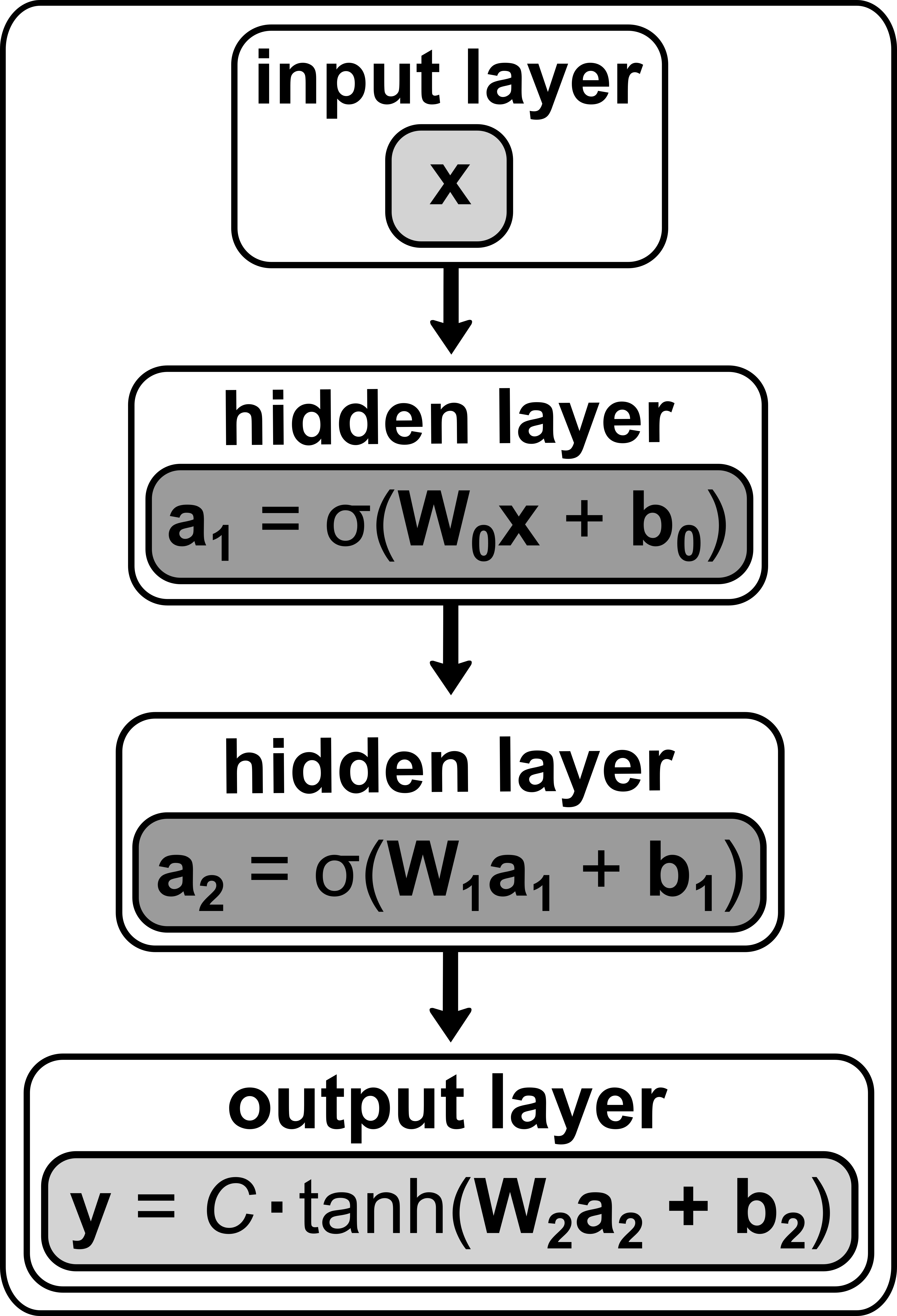
Figure 3: Schematic diagram of the NN architecture. The activation vector of each hidden layer is a_i. The input and output vectors are $\mathbf{x}$ and $\mathbf{y}$ and the weight matrix and bias vector for each layer are $\mathbf{W}_{i}$ and $\mathbf{b}_{i}$, respectively. The activation function of the hidden layers is $\sigma(\cdot)$ and corresponds to a shifted softplusDugas et al. (2001) function $\sigma(\cdot)=\ln(1+e^{(\cdot)})-\ln(2)$. Here, activation functions act element-wise on input vectors $(\cdot)$. The constant $\ln(2)$ centers the mean activation of the hidden nodes at zero, thereby decreasing the bias shift effect which speeds up the learning.Clevert, Unterthiner, and Hochreiter (2015); LeCun et al. (2012) The activation function of the output layer is $C\cdot\tanh(\cdot)$Glorot, Bordes, and Bengio (2011), where $C$ is an overall scaling with $C=8/12/8$ in the F-, K- and G-based approaches.

For training, the input and output of the NN are standardized according to $x_{i}^{\prime}=(x_{i}-\bar{x}_{i})/\sigma_{i}$, where $x_{i}$, $\bar{x}_{i}$ and $\sigma_{i}$ are the $i$-th input/output, and the mean and standard deviation of their distribution over the entire set of training data. Scaling of the input, here by means of standardization, is common practice in the data pre-processing step for machine learning tasks relying on gradient descent for optimization, as it generally yields a faster convergence rate.LeCun et al. (2012) The additional standardization of the output allows one to use a root-mean-square deviation (RMSD) loss function, as the non-standardized values can differ drastically in magnitude and spread. Thus, in particular low and high product state probabilities can be predicted with similar accuracy. It would also be possible to simply normalize the output but the additional offset gives the flexibility to use a scaled hyperbolic tangent as an activation function for the output layer which increases the NN prediction accuracy compared to other/no activation functions. The RMSD loss function $\mathcal{L}$ used here is

$$\mathcal{L}=\sqrt{\frac{1}{N}\sum\limits_{i=1}^{N}\left(y_{i}-y^{\prime}_{i}\right)^{2}},$$ (11)

with $y_{i}$ and $y^{\prime}_{i}$ the predicted and reference output values.

The weights and biases of the NN are initialized according to the Glorot schemeGlorot and Bengio (2010) and optimized using AdamKingma and Ba (2014) with an exponentially decaying learning rate. The NN is trained using TensorFlow Abadi et al. (2016) and the set of weights and biases resulting in the lowest loss as evaluated on the validation set are used for predictions. When training a NN using Set1 with $N_{\text{tot}}=3698$ data sets, $N_{\text{train}}=3000$ were randomly selected for training, $N_{\text{valid}}=600$ for validation and $N_{\text{test}}=98$ as a test set, whereas for Set2 $N_{\text{tot}}=4658$, $N_{\text{train}}=3600$, $N_{\text{valid}}=900$, and $N_{\text{test}}=158$.

To train models on reactant state distributions that can not be characterized as a single set of temperatures $\bm{T}$, Set3 was constructed by means of a weighted sum of the distributions in Set2 (see Section II.2). For this, 158 data sets are randomly selected from $N_{\text{tot}}=4658$ data sets of Set2. They constitute the subset from which the final test set of Set3 is generated. Here, $N_{\text{test}}=125$, see Section II.2. The remaining 4500 data sets make up the subset from which the data sets for training and validation are constructed. In particular, $N_{\text{train}}+N_{\text{valid}}=5000,10000,15000,20000,25000,30000$ data sets are generated by means of the same procedure, making up the final training and validation sets of Set3 with $N_{\text{train}}=0.8\times(N_{\text{train}}+N_{\text{valid}})$ and $N_{\text{valid}}=0.2\times(N_{\text{train}}+N_{\text{valid}})$. All NNs in this work were trained on a 1.8 GHz Intel Core i7-10510U CPU with training times shorter than 10 minutes.

III Results

The results section first presents DTD models for the F-, K-, and G-based approaches for $T_{\text{vib}}=T_{\text{rot}}$. This is followed by discussing the influence of featurization, computational cost and generalizability of the approaches considered. As the G-based approach is found to perform best from a number of different perspectives, models are then trained for $T_{\text{vib}}\neq T_{\text{rot}}$ and for nonequilibrium reactant state distributions. Also, variations of the G-based approach requiring fewer input data are explored. Then, the findings are discussed in a broader context and conclusions are drawn.

III.1 Distribution-to-Distribution Models for $T_{\text{vib}}=T_{\text{rot}}$

First, an overall assessment of the three different approaches for describing the reactant state distributions for Set1 (i.e. $T_{\text{vib}}=T_{\text{rot}}$) is provided. As they are generated according to the typical sampling procedures followed by QCT simulations and not from direct function evaluations of equilibrium distributions they contain noise. This is done because the entire work is concerned with a situation typically encountered in QCT simulations of reactive processes.Karplus, Porter, and Sharma (1965) Also, it is noted that for the reactant state distributions one should find - as demonstrated here - that they are characterized by one parameter only, namely temperature. This, however, is an open point and not guaranteed for the product state distributions, which are nonequilibrium distributions in general.

For the F- and K-based approaches the reactant state distributions are first represented either as a parametrized model function or as a RKHS, respectively, and the agreement is found to be excellent (see Figures 1 and 2). For the G-based approach this step is not required, as the input are the amplitudes of the reactant state distributions themselves (see Figure 2).

Having established that all three (F-, K-, and G-based) approaches are suitable to describe reactant state distributions, a NN for each of the three models was trained on Set1 with $N_{\text{train}}=3000$ and $N_{\text{valid}}=600$. The quality of the final model for predicting product state distributions depends on two aspects: 1. The ability of the NN to learn and predict the product state distributions obtained from the QCT simulations 2. The ability of the (F-, K- or G-based) approaches to describe these distributions.

1. Quality of the NN Prediction: For the first aspect, RMSD and coefficient of determination ($R^{2}$) values, referred to as RMSD_NN and $R^{2}_{\rm NN}$, are considered as performance measures. For a single data set from the test set these are calculated by comparing the normalized reference representations of each of the models and the corresponding normalized NN predictions on the grid for which QCT data is available for each of the three product state distributions separately and averaging over the resulting values. The normalization factors were calculated by numerical integration of the distributions obtained from the QCT simulations. The final RMSD and $R^{2}$ values are then obtained by averaging over the entire test set with $N_{\text{test}}=98$, see Table 1.

DTD model	${\rm RMSD}_{\rm NN}$	${R^{2}}_{\rm NN}$	${\rm RMSD}_{\rm QCT}$	${R^{2}}_{\rm QCT}$
F-NN	0.0007	0.9996	0.0014	0.9982
K-NN	0.0013	0.9984	0.0014	0.9981
G-NN	0.0009	0.9994	0.0010	0.9991

Table 1: Performance measures of the F-, K- and G-based models (F-NN, K-NN and G-NN) trained and evaluated on Set1. The number of significant digits being reported is based on the findings of Table S2.

For three different data sets from the test set, the results from explicit QCT simulations, the NN predictions, and the reference representation of the corresponding approach are shown in Figure 4. These results are representative of NN predictions for data from the test set for each of the three approaches as they are characterized by an $R^{2}_{\rm NN}$ value closest to the mean $R^{2}_{\rm NN}$ value as evaluated over the test set. Figures S1 and S2 show the predictions that are characterized by the highest (“accurate” prediction) and lowest (“inaccurate” prediction) $R^{2}_{\rm NN}$ value in the test set, respectively.

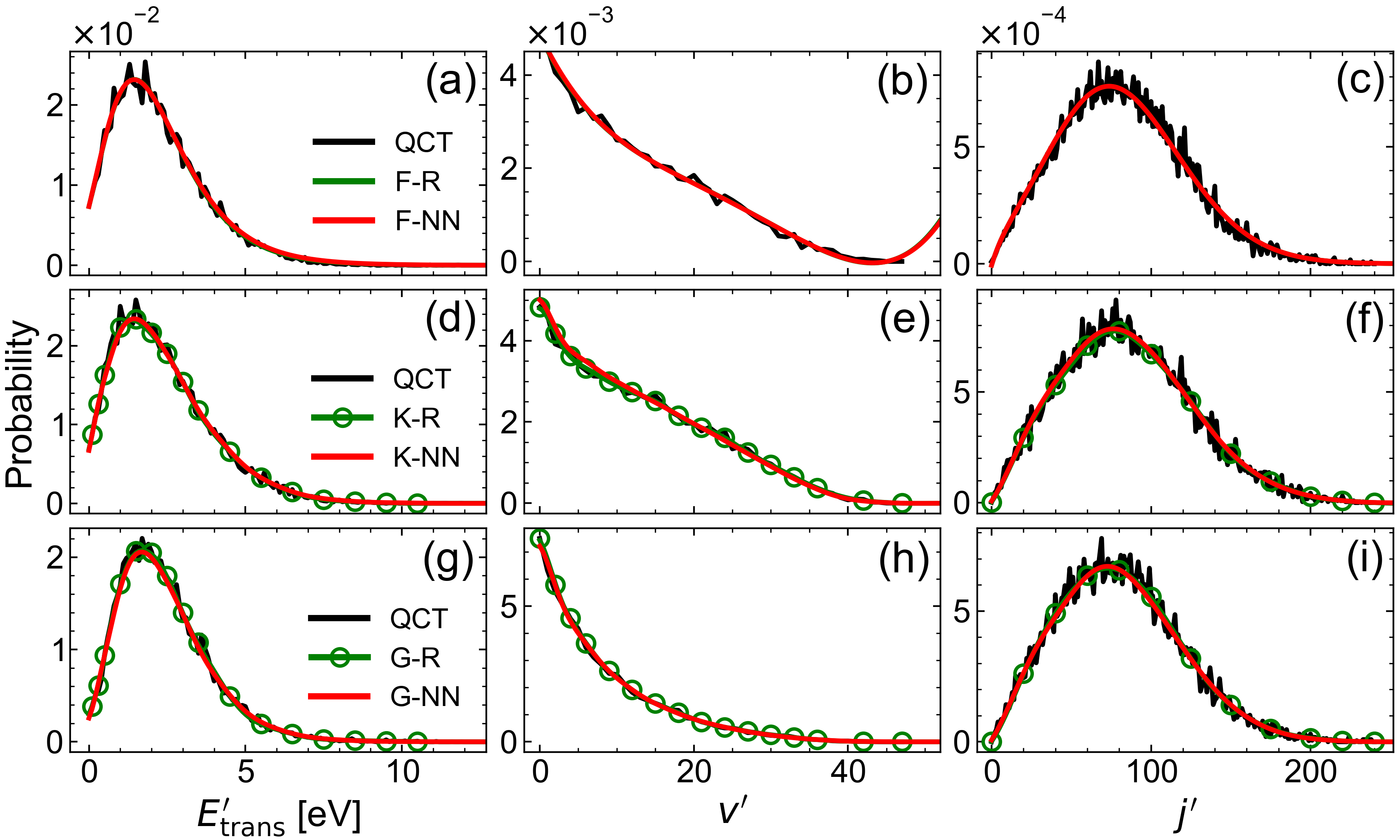
Figure 4: Product state distributions obtained by explicit QCT simulations (QCT) as well as the corresponding references (-R) and predictions (-NN) from the (a-c) F-based (F-R, F-NN), (d-f) K-based (K-R, K-NN) and (g-i) G-based approaches (G-R, G-NN). Also, the amplitudes to construct the reference RKHS-based representations in the K- and G-based approaches are displayed (circles). The data sets considered here are from the test set of Set1 and result in predictions that are characterized by an $R^{2}_{\rm NN}$ value closest to the mean $R^{2}_{\rm NN}$ value as evaluated over the test set: (a-c) $\bm{T}=($9500 K, 16000 K, 16000 K), RMSD${}_{\text{NN}}=0.0005$, $R^{2}_{\text{NN}}=0.9996$, (d-f) $\bm{T}=($10250 K, 19250 K, 19250 K), RMSD${}_{\text{NN}}=0.0013$, $R^{2}_{\text{NN}}=0.9984$, (g-i) $\bm{T}=($12000 K, 9750 K, 9750 K), RMSD${}_{\text{NN}}=0.0009$, $R^{2}_{\text{NN}}=0.9994$.

In general, all three approaches are very accurate, as their predictions closely match the corresponding reference representations. Closer inspection of Figure 4 reveals that for these particular examples the K-based approach appears to yield slightly less accurate predictions than the other two approaches (see, for example Figure 4f). The RMSD_NN values are 0.0007, 0.0013 and 0.0009 for the F-, K-, and G-based models respectively, and the corresponding $R^{2}_{\rm NN}$ values are 0.9996, 0.9984 and 0.9994. These performance measures indicate that the F-based approach yields the most accurate predictions, followed by the G- and K-based approaches.

2. Quality of the F-, K-, and G-Based Model Predictions: For the product state distributions the prediction accuracy depends on the accuracy of the NN and the accuracy with which the representations approximate them. Figure 5 compares the final model predictions from the three approaches. The examples illustrate the variety of product state distributions in Set1. It is found that despite the appreciable variation in shapes (in particular for $P(v^{\prime})$) all three models correctly describe the product state distributions. Distributions $P(v^{\prime})$ are not well represented as a single equilibrium distribution which is typical for vibrational states at high temperatures.Boyd (2015); Singh and Schwartzentruber (2018)

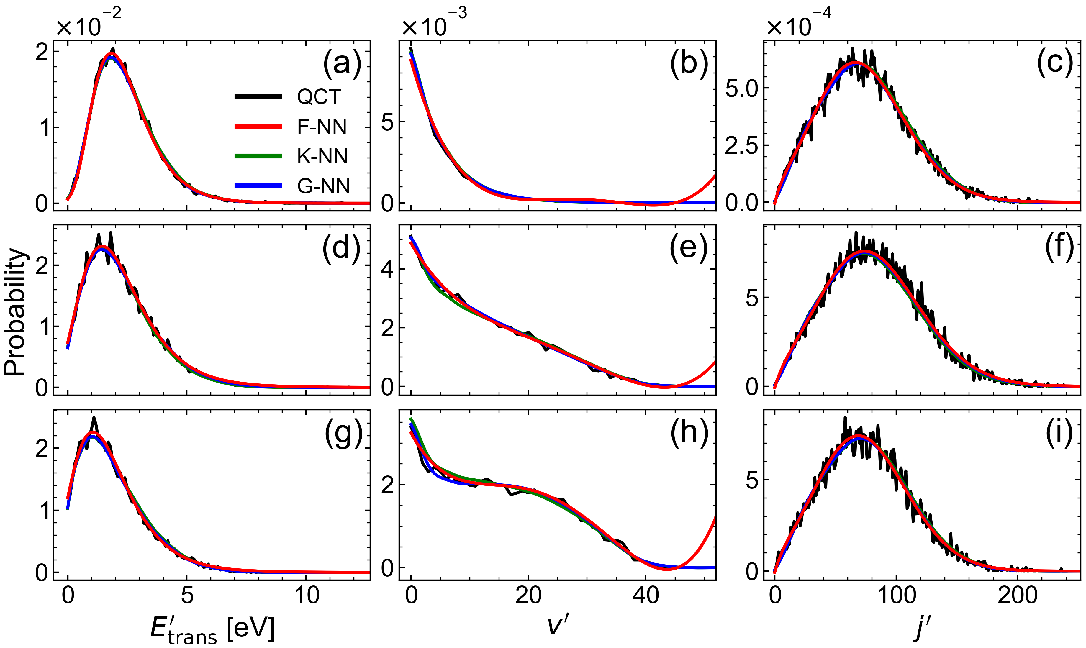
Figure 5: Product state distributions obtained by explicit QCT simulations (QCT) as well as the corresponding model predictions obtained in the (a-c) F-based (F-NN), (d-f) K-based (K-NN) and (g-i) G-based approaches (G-NN). The data sets considered here are from the test set of Set1: (a-c) $\bm{T}=$ (12500 K, 5750 K, 5750 K) , (d-f) $\bm{T}=$ (9500 K, 16000 K, 16000 K), (g-i) $\bm{T}=$ (5750 K, 19250 K, 19250 K).

A quantitative measure for the performance of the three models are the RMSD and $R^{2}$ values calculated by comparing the locally averaged ($n_{\text{max},E_{\rm trans}^{\prime}}=3$, $n_{\text{max},v^{\prime}}=2$, $n_{\text{max},j^{\prime}}=10$) QCT data and the model predictions following a similar procedure as for RMSD_NN and $R^{2}_{\rm NN}$ which will be called RMSD_QCT and $R^{2}_{\rm QCT}$, respectively. For Set1 these performances are reported in Table 1. Again, all models are of high quality with the G-based approach performing best. The somewhat lower quality of the F-based approach when compared to the G-based approach can largely be attributed to the fits of the product state distributions. The representation of the F-based approach leads to differences, in particular for $P(v^{\prime})$ (e.g., deviations for small and high $v^{\prime}$ or extra undulations in Figure 5b). However, the deviations in the F-based approach observed for high $v^{\prime}$ are only partially relevant, as the accessible vibrational and rotational state space is finite in practice, here $v^{\prime}_{\rm max}=47$, $j^{\prime}_{\rm max}=240$. Since state space is limited, extrapolation is not always required. Considering the K- and G-based approaches, the reference representations describing product distributions are nearly identical and reproduce the QCT data very closely. Hence, the lower accuracy of the final model in the K-based approach when compared to the G-based approach can largely be attributed to its lower NN prediction accuracy.

For the F-based approach, finding an optimal set of model functions (Eqs. 2 to 7) specific to the system at hand is expected to be a difficult task. Such parametric models for nonequilibrium conditions are still a current topic of research.Singh and Schwartzentruber (2018, 2020c, 2020a) To highlight the performance of different models, a parametric model for transient vibrational and rotational state distributions based on surprisal analysisSingh and Schwartzentruber (2018) was applied to Set1. $P(v^{\prime})$ and $P(j^{\prime})$ distributions for two different sets of temperatures (($T_{\text{trans}}=20000$ K, $T_{\text{rovib}}=5000$ K) and ($T_{\text{trans}}=5500$ K, $T_{\text{rovib}}=20000$ K)) from QCT simulation are modelled following the parametrization of Ref. (9) (see Figure S3). While for the first set of temperatures (translationally hot and rovibrationally moderately hot) the QCT results for $P(v^{\prime})$ and $P(j^{\prime})$ are closely matched by the model, for the second set (translationally moderately hot and rovibrationally hot) both distributions are insufficiently described by the model, in particular for $P(v^{\prime})$ which is consistent with Ref. (9). The fact that the shape of the $P(v^{\prime})$ appears to vary more widely for different $\bm{T}$ compared to $P(E_{\rm trans}^{\prime})$ and $P(j^{\prime})$ could be a partial explanation of why developing a universally valid parametric model for $P(v^{\prime})$ is more challenging. It should be emphasised that comparison between predictions based on the model and explicit QCT simulations is mandatory to validate the model function used.

III.2 Sensitivity of Performance to Feature Selection

As in all machine learning tasks, feature selection for representing the raw data is crucial for the complexity and prediction accuracy of the resulting NN-based model.Goodfellow, Bengio, and Courville (2016); Bengio, Courville, and Vincent (2012) Here, the main difference between the three approaches are the features that represent reactant and product state distributions and which serve as input/output of the NNs. Hence, any difference in the NN prediction accuracy is due to the features used (i.e. the “featurization”). Here, the features are fitting parameters (F-based), kernel coefficients (K-based), and amplitudes (G-based) and together they constitute a feature vector. Hence, a good featurization allowing for an accurate NN to be trained is characterized by the fact that similarly shaped distributions are described by similar feature vectors.Faber et al. (2015) Here, “similarity” is measured by an appropriate metric, such as an Euclidean norm.

For the F-based approach, the choice of model functions (see Eqs. 2 to 7) turned out to yield a satisfactory featurization. Conversely, for the K-based approach it was necessary to increase the regularization rate $\lambda$ and averaging over more neighbouring data points which in essence smooths out sharp variations in the kernel coefficients between neighboring data sets in temperature space. In the G-based approach, accurate NN predictions were obtained through local averaging because the amplitudes are the features.

For the F-based approach the dependence of NN performance on feature selection was explicitly explored by choosing an alternative parametrization for

$$\tilde{P}(v^{\prime})=g_{1}\exp(-(\ln(2g_{2}(v^{\prime}-g_{3})/g_{4}+1)/g_{2})^{2})+g_{5}\exp(-(\ln(2g_{6}(v^{\prime}-g_{7})/g_{8}+1)/g_{6})^{2}),$$ (12)

where $\bm{g}=(g_{1},...,g_{8})$ are the corresponding fitting parameters. The resulting fit (see Figure S4) to the QCT data demonstrates that Eq. 12 yields a better fit than Eq. 6. However, training the corresponding NN turned out to be difficult and the resulting NN predictions were highly inaccurate (see below).

Figure 6 illustrates these points for $P(v^{\prime})$ for three combinations of simulation temperatures with 1) $T_{\text{trans}}\sim T_{\text{rovib}}$ ($T_{\text{trans}}=5000$ K, $T_{\text{rovib}}=5000,5250,5500,5750$ K; black) 2) $T_{\text{trans}}<T_{\text{rovib}}$ ($T_{\text{trans}}=5000$ K, $T_{\text{rovib}}=10000,10250,10500,10750$ K; red), and 3) $T_{\text{trans}}>T_{\text{rovib}}$ ($T_{\text{trans}}=12000$ K, $T_{\text{rovib}}=5000,5250,5500,5750$ K; green). As Figure 6a demonstrates, the shapes of all $P(v^{\prime})$ are comparable and for each color there are four largely overlapping distributions which can not be separated because the differences in $T_{\text{rovib}}$ are too small. Using the F-based approach with Eq. 6 for $P(v^{\prime})$ yields parameter values that are clustered (Figure 6b) for the black, red, and green $P(v^{\prime})$, respectively. For such input a robust NN can be trained. Conversely, using Eq. 12, even the fitting parameters for one set of $P(v^{\prime})$ spread considerably and mix with those from $P(v^{\prime})$ of other temperature combinations, see Figure 6c. Thus, similarity in the shape of $P(v^{\prime})$ does not translate into similarity of the fitting parameters used for the featurization. This is an unfavourable situation for training a NN which compromises the prediction ability of such an F-based model. The F-based model trained with Eq. 6 yields an accurate prediction (${\rm RMSD}_{\rm NN}=0.0007,R^{2}_{\rm NN}=0.9996$) whereas the one trained with Eq. 12 fails to predict $P(v^{\prime})$ (RMSD${}_{\rm NN}=0.0348$, $R^{2}_{\rm NN}=-10.6133$; i.e., this model is worse than a baseline model with $R^{2}=0$). Similarly, a K-based approach can lead to considerable spread of the kernel coefficients (Figure 6d) which is not observed for the amplitudes in the G-based approach (Figure 6e). Such differences in the featurization leads to differences in the NN prediction accuracies.

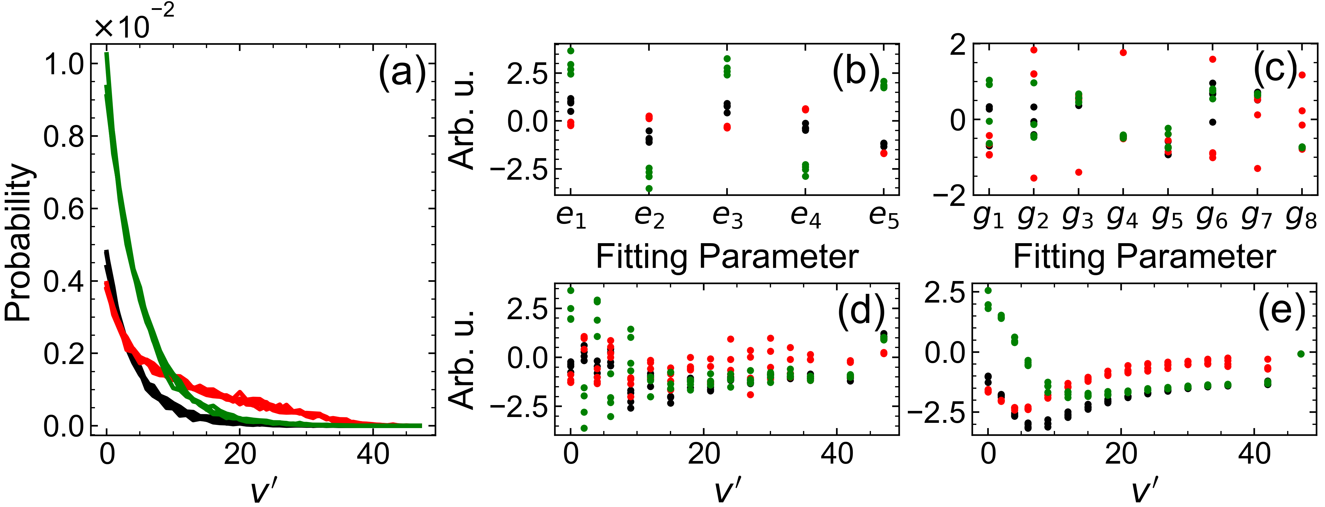
Figure 6: Comparison of the featurization for three different groups of similarly shaped $P(v^{\prime})$ (black, red and green). Panel a: the distributions as obtained from QCT simulations (fluctuating lines). Panels b and c: Fitting Parameters for the F-based approach with model functions from Eqs. 6 and 12; panel d: kernel coefficients for the K-based approach and panel e: amplitudes for G-based approach. The temperatures are ($T_{\text{trans}}=5000$ K, $T_{\text{rovib}}=5000,5250,5500,5750$ K; black), ($T_{\text{trans}}=5000$ K, $T_{\text{rovib}}=10000,10250,10500,10750$ K; red), and ($T_{\text{trans}}=12000$ K, $T_{\text{rovib}}=5000,5250,5500,5750$ K; green). The quality of all fits in panel a is as good as in Figure 5 and all features are standardized.

Another difference between the NNs in the three approaches is the fact that prediction errors in the features translate into errors in the corresponding predicted product state distributions in different ways. For the G-based approach, an error in the predicted features directly translates into an error in the predicted product state distributions. This is not the case for the F- or K-based approaches. As an example, the model functions for the product state distributions in an F-based approach depend nonlinearly on the fitting parameters (features). Hence, small errors in the NN predictions can lead to large errors in the predicted distributions. This is problematic, as the NNs are trained on a loss function that measures the errors in feature space, whereas one is rather interested in the quality of the predicted product state distributions. By using a loss function that depends on errors in the predicted product distributions this problem can be avoided. In the K-based approach this is partially resolved by the choice of a Gaussian kernel where the hyperparameter $\sigma$ is assigned according to the procedure described in Section II.4. This results in a local kernel with kernel coefficients largely determined by the amplitude at the corresponding grid points and its nearest neighbours.Bengio, Delalleau, and Roux (2006) Consequently, errors in the predicted kernel coefficients are also restricted to impact the predicted model function locally, similar to the G-based approach.

III.3 Computational Cost and Generalizability

To compare the computational cost of the final models in the F-, K- and G-based approaches, the evaluation times of the final models for 1000 randomly selected data sets (from Set1) are considered. Here, a single evaluation is defined as a prediction of the product ($E_{\text{trans}}^{\prime},v^{\prime},j^{\prime}$) distributions at 201, 48 and 241 evenly spaced points in the interval between $E_{\text{trans}}^{\prime}=0-20$ eV, $v^{\prime}=0-47$ and $j^{\prime}=0-240$, respectively, given the reactant state distributions. The evaluation times on a 1.8 GHz Intel Core i7-10510U CPU are $(9.0\pm 0.1)$ s, $(29.0\pm 0.3)$ s, and $(28.9\pm 0.3)$ s for the F-, K- and G-based models, respectively. For the F-based approach the evaluation time is 3 times faster compared to the two other methods and is dominated by fitting the reactant state distributions to Eqs. 2 to 4 whereas for the K- and G-based approaches the evaluation time is dominated by the evaluation of the RKHS-based representations of the product distributions given the predicted kernel coefficients or amplitudes, respectively. This may be further improved for the K- and G-based approaches by using a computationally efficient kernel toolkit.Unke and Meuwly (2017)

In terms of generality and transferability, an F-based model can not be easily generalized to distributions with widely different shapes emanating from the QCT simulations. New optimal model functions, also suitable for training a NN would need to be found for every single system. Conversely, with the K- and G-based approaches all desired features of the distributions can be captured by an appropriate choice of reproducing kernel and grid, requiring fine-tuning of the corresponding hyperparameters. Compared to the K-based approach, a G-based model only requires tuning of the corresponding hyperparameters for the product state distributions. In addition, for a G-based model it is also possible to use a linear interpolation instead of a RKHS if one is not concerned with extrapolation. Then, the grid for the product state distributions needs to be chosen sufficiently dense suitable for linear interpolation at the cost of an increased number of NN parameters.

III.4 Grid-Based Models for $T_{\text{vib}}\neq T_{\text{rot}}$

As vibrational relaxation is often slow in hypersonic flow, assuming $T_{\text{vib}}=T_{\text{rot}}$ is often not a good approximation.Boyd (2015); Bender et al. (2015) Therefore, the G-based approach is extended to and tested for the case of $T_{\rm vib}\neq T_{\rm rot}$ using Set2. Restricting this to the G-based approach is motivated by the fact that it performed best so far, both in terms of final model accuracy and practicability.

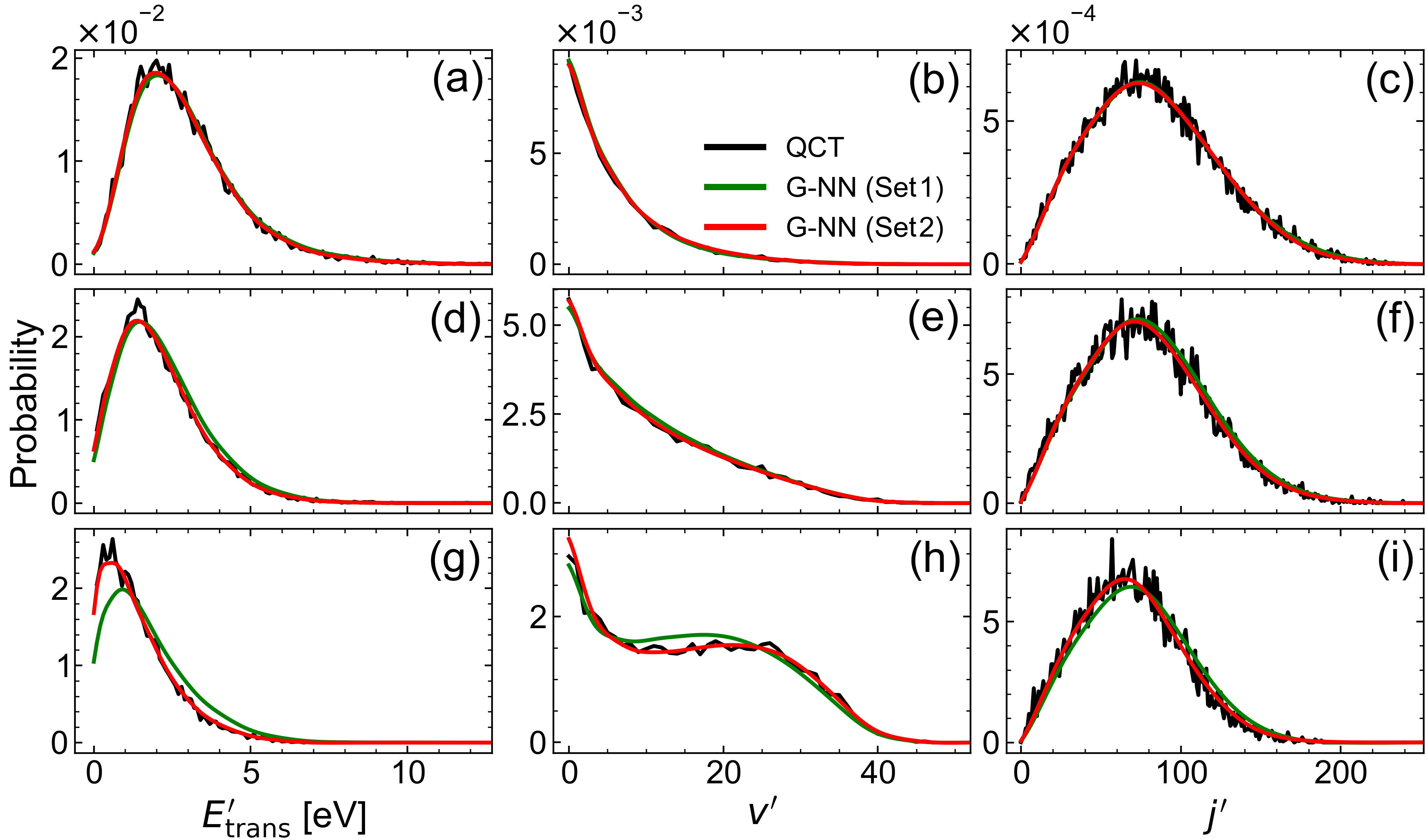
Figure 7: Performance of the G-based approach on Set2 from training on Set1 (green) or Set2 (red). Product state distributions from explicit QCT simulations (QCT) compared with model predictions from the G-based approach by training on Set1 (G-NN (Set1)) and Set2 (G-NN (Set2)) for: (a-c) $\bm{T}$ = (20000 K, 7000 K, 5000 K) , (d-f) $\bm{T}$ = (10000 K, 14000 K, 9000 K), (g-i) $\bm{T}$ = (5000 K, 20000 K, 8000 K).

First, predictions for Set2 were made based on the G-based model (G-NN) trained on Set1 ($T_{\text{vib}}=T_{\text{rot}}$) and compared with QCT data (QCT), see Figure 7. The accuracy of this G-based model deteriorates (see Table S3 for all performance measures) as the difference between $T_{\text{vib}}$ and $T_{\text{rot}}$ increases (green lines in Figure 7). Consequently, a new G-based model was trained and evaluated on Set2. The resulting model predictions (red lines in Figure 7) are very accurate, close to the level of accuracy of the G-based model trained and evaluated on Set1. Thus, the G-based approach performs equally well for $T_{\text{vib}}=T_{\text{rot}}$ and $T_{\text{vib}}\neq T_{\text{rot}}$.

In an attempt to further improve the G-based approach, three alternative types of input were considered. They are all based on reducing the number of input which not only decreases computational cost, but also removes redundant features which can improve prediction accuracy.Chandrashekar and Sahin (2014) Again, continuous distributions were obtained from an RKHS of the discrete predictions. The first (G^′-based) model used values of the reactant state distributions at a fixed but reduced number of grid points compared with the G-based model used so far (see Table S1). Next, a model using only the three temperatures characterizing the reactant state distributions $\bm{T}$ as input (G($\bm{T}$)-based model) is considered. This is meaningful because the value of $\bm{T}$ entirely specifies the equilibrium reactant state distributions. A third model used averages $\bm{\mu}=(\mu_{E_{\rm trans}},\mu_{v},\mu_{j})$ of the reactant state distributions as input (G($\bm{\mu}$)-based model). For generality, these models will be trained and evaluated on Set2 and all performance measures are summarized in Table S3.

A G^′-based approach using two grid points per reactant state distribution ($E_{\text{trans}}=0.3,3.5$ eV; $v=2,12$; $j=30,150$) still allows for accurate predictions of the product state distributions. The location of these grid points is largely arbitrary, but they should be sufficiently spaced to provide information about the distribution at different locations. However, reducing to a single grid point per reactant state distribution ($E_{\text{trans}}=0.6$ eV, $v=6$, $j=60$) leads to a significant drop in the prediction accuracy. The fact that 2 grid points per reactant state distribution are required for accurate predictions can mainly be attributed to the presence of noise in the distributions arising from finite sample statistics (see Section IV in SI for further clarification). The resulting predictions for the above mentioned models for selected data sets from the test set are displayed in Figure S6 in the SI.

For the G($\bm{T}$)-based model the performance is close to the original G-based model trained and evaluated on Set2. This is expected, as $\bm{T}$ entirely specifies the equilibrium reactant state distributions and allows a NN to predict corresponding product state distributions. Finally, providing the mean $\mu$ of each of the reactant state distributions as input in a G($\bm{\mu}$)-based model also leads to highly accurate predictions. This can be explained by the fact, that the mean values $\bm{\mu}$ of the reactant equilibrium distributions are uniquely linked to the corresponding set of temperatures $\bm{T}$.

The results of this Section highlight that all three variants of the G-based model yield similarly high levels of accuracy as the G-based approach, which makes them preferable as they are computationally less expensive. These results may be specific to reactant state distributions that can be uniquely specified by a single parameter, such as a temperature or its mean value $\mu$. To explore this and to further demonstrate the generality of the G-based approach and its variants, a more diverse dataset for nonequilibrium conditions (Set3) was finally considered, for which the reactant state distributions are characterized by multiple sets of temperatures $\bm{T}$.

III.5 Grid-based Models for Nonequilibrium Product State Distributions

As a final application, nonequilibrium DTD models are constructed for Set3 which was generated by means of a weighted sum (see Eq. 1) using Set2 (see Section II.2) with $N\in[2,3]$, and $w_{n}\in[1,2]$. Training and validation sets of variable sizes were considered, whereas $N_{\text{test}}=125$ throughout. First, a G-based model was trained on Set3 with $N_{\text{train}}+N_{\text{valid}}=5000$. Again, all performance measures are summarized in Table S3.

The predictions of this G-based model for three different data sets from the test set are shown in Figure 8. In particular, the predictions for these three data sets are characterized by a $R^{2}_{\rm QCT}$ value closest to the mean $R^{2}_{\rm QCT}$ value as evaluated over the entire test set, as well as the highest and lowest $R^{2}_{\rm QCT}$ value in the test set, respectively. Once again, the G-based approach gives a very accurate DTD model, close to the G-based model trained and evaluated on Set2. However, the predictions of the G-based model for Set3 have a larger variance compared to the G-based model for Set2. To assess the influence of the training and validation set size on the prediction accuracy, a learning curve was computed (Figure S7). The NN prediction accuracy does not significantly increase when $N_{\text{train}}+N_{\text{valid}}$ was increased from 5000 to 30000 in increments of 5000. Hence, this justifies training and validating the variants of the G-based model only on $N_{\text{train}}+N_{\text{valid}}=5000$.

In an attempt to further improve and reduce this model for Set3, the dependence on different amount of input information (as was done for Set2) was tested again. Accurate predictions are still possible with amplitudes of $P(E_{\text{trans}}),P(v),P(j)$ at three different grid points ($E_{\text{trans}}=0.3,1.5,3.5$ eV; $v=2,6,12$; $j=30,60,150$), but the prediction accuracy decreases when reducing this to two grid points ($E_{\text{trans}}=0.3,3.5$ eV; $v=2,12$; $j=30,150$). Again it is found that with a G^′-based approach the number of grid points characterizing the reactant state distributions can be significantly reduced compared to the grids in Table S1. This suggests that the possibility to reduce the number of input features (amplitudes) in such G-based models is a generic property which can be systematically explored.

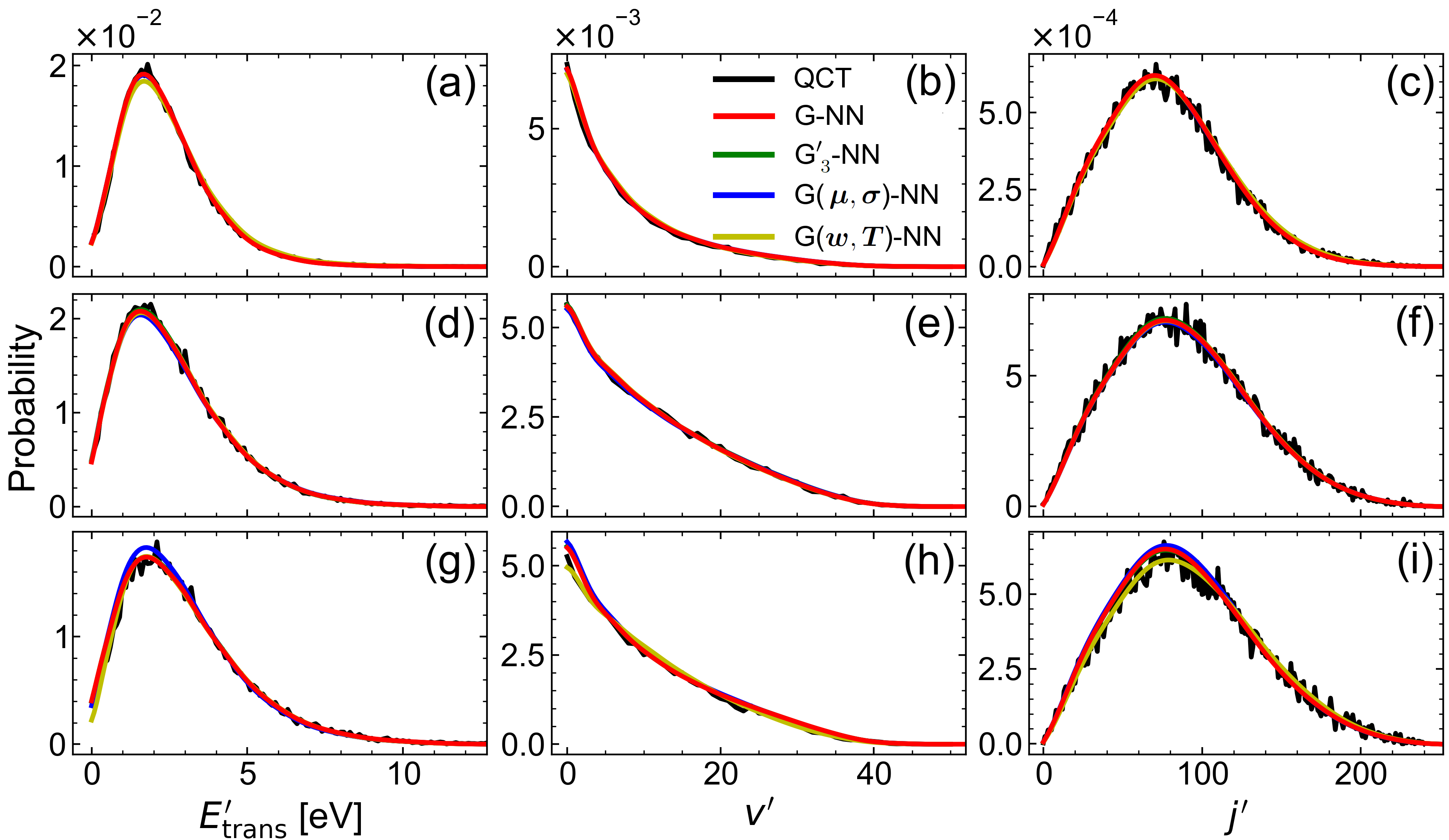
Figure 8: Performance of G-based models and variants trained and evaluated on Set3. Product state distributions obtained from explicit QCT simulations (QCT), together with the predictions from the G- (G-NN), G${}^{\prime}_{3}$- (G${}^{\prime}_{3}$-NN), G($\bm{\mu},\bm{\sigma}$)- (G($\bm{\mu},\bm{\sigma}$)-NN) and G($\bm{w},\bm{T}$)-based (G($\bm{w},\bm{T}$)-NN) models trained on Set3. G${}^{\prime}_{3}$-NN uses 3 grid points per reactant state distribution (see text). The data sets considered here are from the test set of Set3. In particular, the predictions for these three data sets are characterized by (a-c) a $R^{2}_{\rm QCT}$ value closest to the mean $R^{2}_{\rm QCT}$ value as evaluated over the entire test set, as well as (d-f) the largest and (g-i) smallest $R^{2}_{\rm QCT}$ value in the test set, respectively. The normalized weights $w_{n}/w_{\rm tot}$ and sets of temperatures $\bm{T}$ characterizing the data sets displayed here are given in Table S4.

Providing the mean $\mu$ and standard deviation $\sigma$ for each reactant state distribution ($E_{\text{trans}}$,$v$,$j$) in a G($\bm{\mu},\bm{\sigma}$)-based approach also yields a good model whereas omitting the standard deviations $\bm{\sigma}$ as input information results in a G($\bm{\mu}$)-based model with a significantly lower prediction accuracy. This should be compared with the G($\bm{\mu}$)-based model for Set2 which yielded accurate predictions. The aforementioned differences of the G^′- and G($\bm{\mu}$)-based models for Set2 and Set3 can be attributed to the fact that the reactant state distributions in Set3 show more diverse shapes compared to Set2, which makes it necessary to provide additional information to maintain a high prediction accuracy. In particular, reactant state distributions in Set3 are nonequilibrium distributions and consequently can not be uniquely specified by a single parameter, such as a temperature or its mean value $\mu$, as was the case in Set2. Rather, the G($\bm{\mu},\bm{\sigma}$)-based approach for Set3 showed that the set of reactant state distributions is characterized by specifying ($\bm{\mu},\bm{\sigma}$).

Keeping this in mind, extending the G($\bm{T}$)-based approach to Set3 can be achieved by providing the sets of temperatures $\bm{T}$ from which the particular reactant state distributions of Set3 were generated, together with the set of weights $\bm{w}$ with which these contributed (see Section II.2). This results in a G($\bm{w},\bm{T}$)-based model. To always guarantee the same number of NN input being specified, as expected by the NN used in this work (see Section II.6), zero padding was used. Such a G($\bm{w},\bm{T}$)-based model for Set3 leads to accurate predictions. The predictions of the G^′-, G($\bm{\mu},\bm{\sigma}$)- and G($\bm{w},\bm{T}$)-based model for selected data sets from the test set are also reported in Figure 8.

Interestingly, the G-, G^′- and G($\bm{\mu},\bm{\sigma}$)-based models trained on Set3 can accurately predict the product state distributions when given the reactant state distributions from Set2. The performance measures (see Table S3) were calculated by considering the subset of 158 data sets of Set2 from which the test set of Set3 was generated. Even though these models were trained on reactant state distributions given as a linear combination of two to three equilibrium distributions, they can accurately generalize to equilibrium reactant state distributions. This is not the case for the G($\bm{w},\bm{T}$)-based model, which yields unreliable predictions when applied to the reactant state distributions of Set2. This can be attributed to the zero padding. In particular, such a model can not generalize at all to reactant state distributions being composed of more than three equilibrium distributions, as this requires more NN input to be specified than there are input nodes. This point can be addressed in the future by considering a different NN architecture, allowing for a variable input size.

Conversely, generalizing to reactant state distributions being composed of more than three equilibrium distributions is possible for the G-, G^′- and G($\bm{\mu},\bm{\sigma}$)-based models trained on Set3. Specifically, a set of 125 reactant and product state distributions given as a linear combination of $N\in[1-10]$ distributions from Set2 (i.e., from the subset of 158 data sets of Set2 from which the test set of Set3 was generated) with integer weights $w_{n}\in[1-100]$ (see Section II.2) was generated, referred to as Set3A. When applied to the reactant state distributions of Set3A, these models still predict the corresponding product state distributions with high accuracy, see Table S3. The final DTD model predictions using the G-based approach as well as its variants for such data sets is shown in Figure 9. Consequently, as discussed in Section II.2, these models are also expected to generalize well to most nonequilibrium distributions encountered in practice.

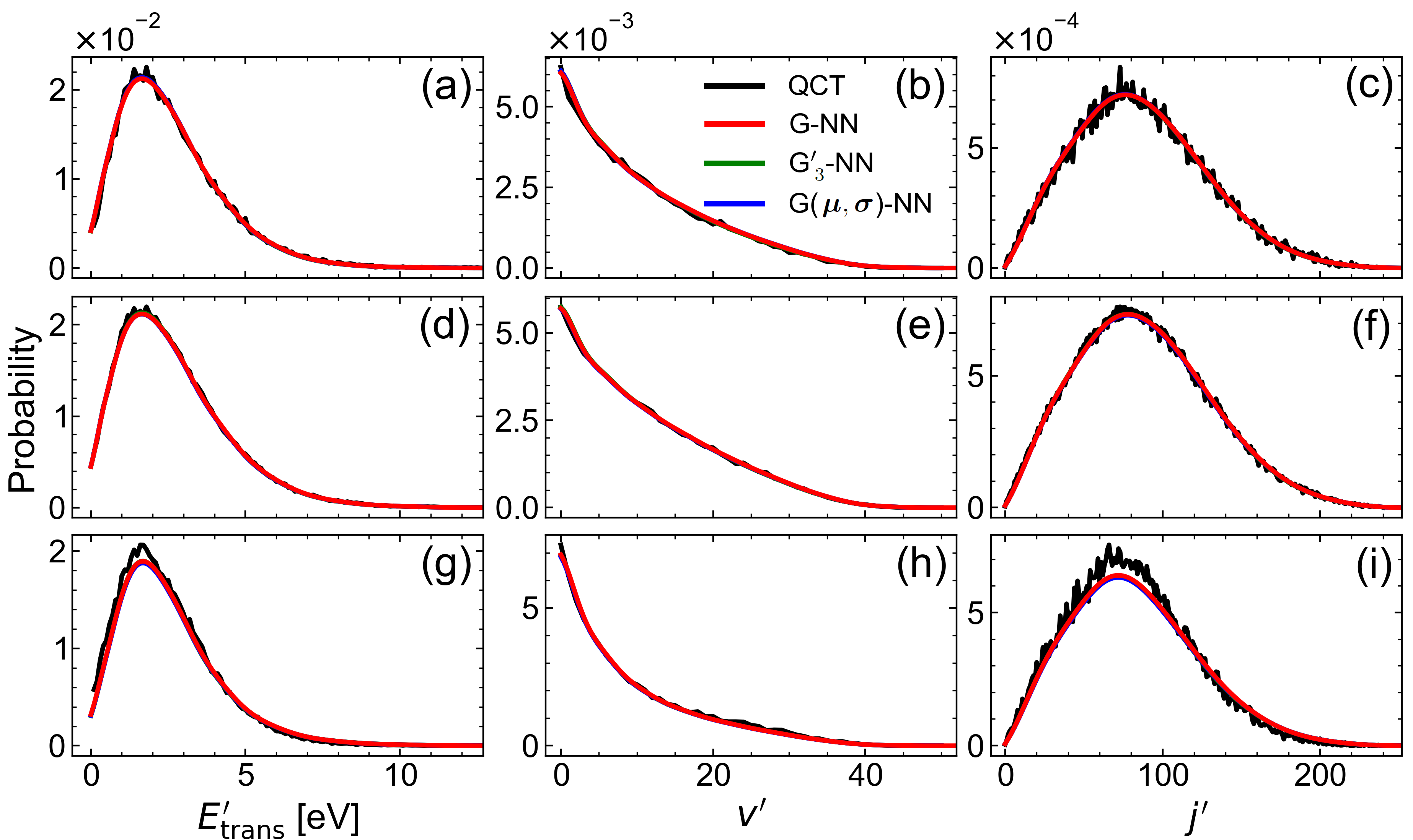
Figure 9: Performance of G-based models and variants trained on Set3 and evaluated on Set3A. Product state distributions obtained from explicit QCT simulations (QCT), together with the predictions from the G- (G-NN), G${}^{\prime}_{3}$- (G${}^{\prime}_{3}$-NN), G($\bm{\mu},\bm{\sigma}$)- (G($\bm{\mu},\bm{\sigma}$)-NN) and G($\bm{w},\bm{T}$)-based (G($\bm{w},\bm{T}$)-NN) models trained on Set3. G${}^{\prime}_{3}$-NN uses 3 grid points per reactant state distribution (see text). The data sets considered here are from Set3A. In particular, the predictions for these three data sets are characterized by (a-c) a $R^{2}_{\rm QCT}$ value closest to the mean $R^{2}_{\rm QCT}$ value as evaluated over the entire Set3A, as well as (d-f) the largest and (g-i) smallest $R^{2}_{\rm QCT}$ value in Set3A, respectively. The normalized weights $w_{n}/w_{\rm tot}$ and sets of temperatures $\bm{T}$ characterizing the data sets displayed here are given in Table S5.

IV Discussion and Conclusions

The present work demonstrates that machine learning of product state distributions from the corresponding reactant state distributions for reactive atom + diatom collisions based on a NN (DTD model) constitutes a promising alternative to a full but computationally very demanding (or even unfeasible, e.g., for diatom + diatom type collisions) treatment by means of explicit QCT simulations. For such DTD models, only a subset of the state space of the reactant needs to be sampled which drastically reduces the computational complexity of the problem at hand.Koner et al. (2019) In particular, DTD models for the N + O₂ $\rightarrow$ NO + O reaction were constructed following three distinct (F-, K- and G-based) approaches for $T_{\rm vib}=T_{\rm rot}$. Although all three approaches yield accurate predictions for the product state distributions as judged from $R^{2}$ and RMSD measures, the G-based approach performs best in terms of prediction accuracy, generality and practical implementation. On the other hand the F-based approach is computationally more efficient by a factor of 3 compared with the K- and G-based approaches. For the K- and G-based approaches it is found that RMSD_NN and $R^{2}_{\rm NN}$ are close to RMSD_QCT and $R^{2}_{\rm QCT}$, respectively. This is different for the F-based approach, where RMSD_NN is smaller than RMSD_QCT by a factor of 2 (similarly for $R^{2}$), see Table 1. This indicates that the parametrizations used for the F-based model can still be improved. In general, an F-based approach is feasible if a universally valid and accurate parametrization for the distributions can be found, which also allows for an accurate NN to be trained. However, finding such a parametrization may not always be possible. Consequently, the G-based approach is generally preferred.

The G-based approach and its input-reduced variants (G^′-, G($\bm{\mu},\bm{\sigma}$)) were found to perform well, too, for $T_{\rm vib}\neq T_{\rm rot}$ (Set2) and nonequilibrium reactant state distributions (Set3 and Set3A). Consequently, the G^′- and G($\bm{\mu},\bm{\sigma}$)-based models are generally preferred over the standard G-based model, as the reduced number of input lowers their computational cost. Moreover, G-, G^′- and G($\bm{\mu},\bm{\sigma}$)-based models trained on Set3 are also expected to generalize well to most realistic nonequilibrium distributions. This is of particular relevance for applications in hypersonics for which nonequilibrium effects are of importance.

Therefore, it is also of interest to discuss the present findings in the context of the methods traditionally employed in DSMCBird (1994) and CFD simulations for hypersonics. Continuum-level reaction rates are required in a multi-temperature framework usually employed in CFD solversGnoffo (1990); Wright, Candler, and Bose (1998); Nompelis, Bender, and Candler . The expression for the exchange reaction rates

$$k_{\rm exc}(\bm{T})=\left(\cfrac{8k_{B}T_{\rm trans}}{\pi\mu}\right)^{1/2}\pi b_{max}^{2}P_{\rm r},$$ (13)

where $k_{B}$ is the Boltzmann constant, $\mu$ is the reduced mass of the reactants. Here, $P_{\rm r}$ is the reaction probability, which can be obtained in a computationally inexpensive way by integrating one of the predicted product state distributions. While rates derived in this manner are based on equilibrium distributions characterized by $\bm{T}$, the vibrational population is nonequilibrium at high temperatures ($T\geq 8000$ K).Singh and Schwartzentruber (2018) Nonequilibrium effects are particularly relevant for diatomic dissociation because high vibrational states have significantly increased probability for dissociation. For instance, for the dissociation of N₂ (in N₂ + N₂) studied in Ref. (20), at $T_{\rm trans}=T_{\rm rot}=10000$ K, the dissociation probability to form N₂ + N + N increases by a factor of 500, when $T_{\rm vib}$ is increased from 8000 K to 20000 K. Conversely, for the exchange reaction considered in the present work, at $T_{\rm trans}=T_{\rm rot}=10000$ K, increasing $T_{\rm vib}$ from 5000 K to 18000 K results in an increase in the reaction rate by only 40 % (see Figure 10). Therefore due to the weaker dependence of the exchange reaction probability on vibrational energy, a Boltzmann distribution at $T_{\rm vib}$ may be sufficient for modeling exchange rates. However, if necessary, the simple model for non-Boltzmann distribution developed in Ref. (25) can be approximated by a linear combination of Boltzmann distributions to include non-Boltzmann effects in the reaction rates for exchange reactions as well. The reactant state distributions can then expressed as a linear combination of equilibrium distributions, as was done here for Set3, from which $P_{\rm r}$ can be calculated. Furthermore, the average vibrational energy change due to decomposition reactions, another key input required in CFD, can also be obtained by taking an appropriate moment of the product state distributions.Singh and Schwartzentruber (2020a)

As an alternative to CFD for hypersonic flow, coarse grained Master equations (ME) are being used for modeling chemical kinetics.Panesi et al. (2013); Magin et al. (2012); Andrienko and Boyd (2017) Here, several rovibrational states are lumped together in groups and only the transition rates between these groups are required which considerably speeds up such simulations. The accuracy of such an approach directly depends on the criterion with which the groups are generated, though.Macdonald et al. (2018a, b) A DTD model as developed here constitutes a new framework for tracking the time evolution of the population in each rovibrational state in a computationally feasible manner. In the context of the present work the DTD model can be repeatedly used for drawing reactant state distributions at each time step for propagating the ME. This is similar to sequential QCT proposed in Refs. Bruehl and Schatz (1988a, b) and DMS method Schwartzentruber, Grover, and Valentini (2018), but computationally more efficient because it avoids explicit trajectory calculations.

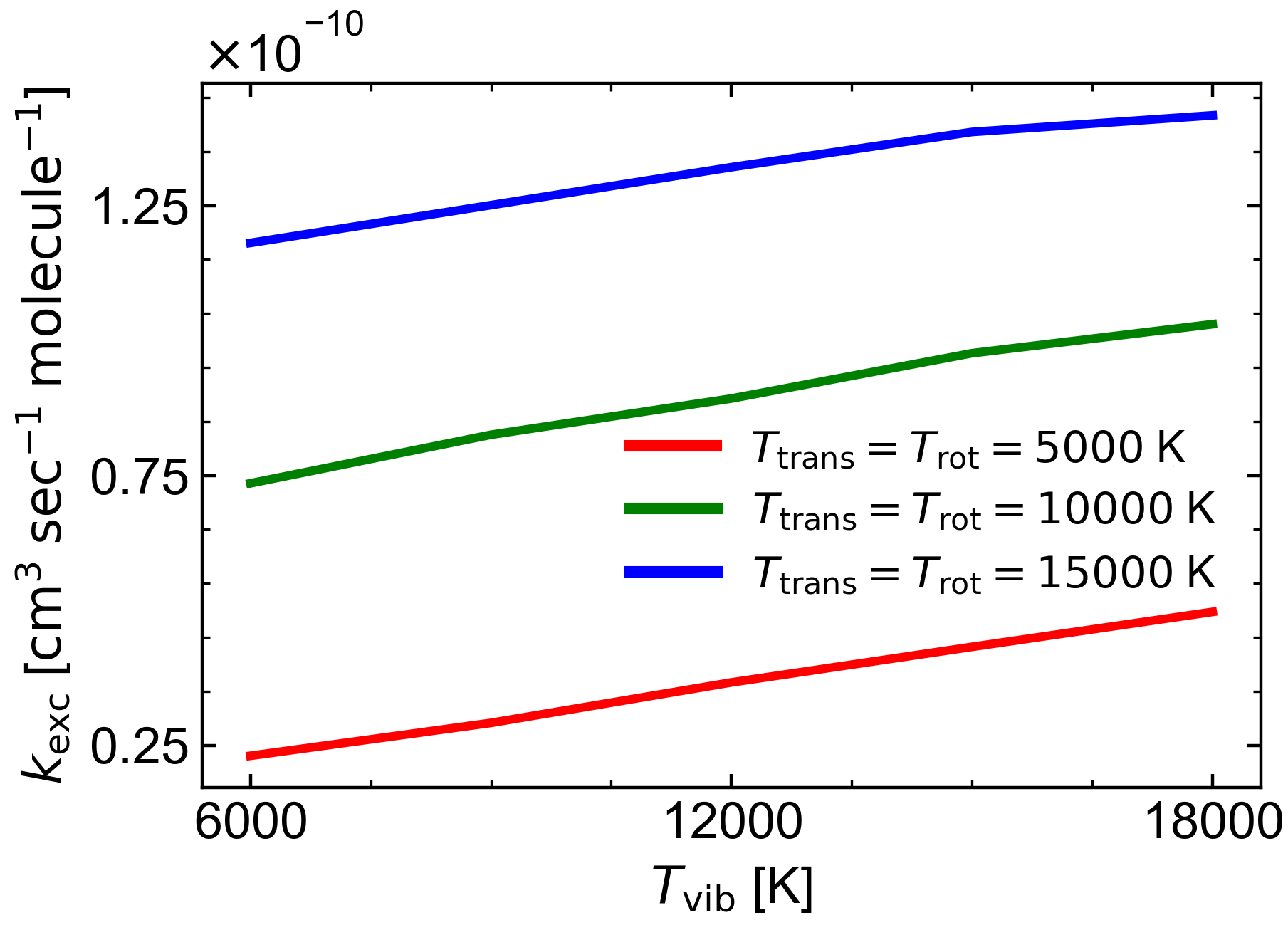
Figure 10: Exchange reaction rates $k_{\rm exc}(\bm{T})$ for N + O₂ $\rightarrow$ NO + O as a function of $T_{\rm vib}$, where $T_{\rm trans}=T_{\rm rot}$.

The product state distributions predicted from the DTD models can also be used for developing simple function-based, state-specific models for exchange reactions in DSMC.Bird (1976); Boyd and Schwartzentruber (2017); Singh and Schwartzentruber (2020c); Gimelshein and Wysong (2017) Such a model can be used within DSMC to estimate state-specific exchange (forward and backward) reaction probabilities instead of the total collision energy (TCE) Bird (1981) model. Furthermore, DTD models also provide a QCT-, physics-based alternative to the phenomenological Borgnakke-Larsen modelBorgnakke and Larsen (1975) which is currently employed to sample internal energy and translational energy of products formed in exchange reactions.

There is scope to further extend and improve the present methods. One of them concerns the application of the G-based models to predict product state distributions which can subsequently be used as reactant state distributions for QCT simulations or DTD models. This way, starting from a set of reactant state distributions transient distributions can be obtained after a certain number of cycles. This will be of particular relevance for applications in hypersonics. Moreover, data construction schemes, such as constructing nonequilibrium distributions as a linear combination of equilibrium distributions, may prove useful for training DTD models from a small set of reactant and product state distributions obtained from explicit QCT simulations that generalize far beyond the conditions used for the reactant state distributions.

Overall, the present work establishes that NN-based models for distribution-to-distribution learning can be developed based on explicit trajectory-based data. This will apply to both, data generated from QCT and quantum simulations if sufficiently converged and complete data can be generated. More generally, the approach presented in this work will also be applicable to situations in which initial distributions are mapped on final distributions by means of a deterministic algorithm such as molecular dynamics simulations. In the future it may also be of interest to consider a fourth approach to DTD learning based on a distribution regression networkKou, Lee, and Ng (2019) promising a higher prediction accuracy with fewer NN parameters compared to the approaches investigated in this work. Moreover, it may also be interesting to explore the possibility for constructing a “state-to-distribution” model which would be intermediate between the DTD model and the earlier STS modelKoner et al. (2019).

Data and Code Availability

All data required to train the NNs has been made available on zenodo https://doi.org/QQQ/zenodo/QQQ and the code for training the DTD models is available at https://github.com/MMunibas/DTD.

V Acknowledgments

This work was supported by the Swiss National Science Foundation through grants 200021-117810, 200020-188724, the NCCR MUST, and the University of Basel.

References

- Park (1993) C. Park, “Review of chemical-kinetic problems of future nasa missions. 1. earth entries,” J. Thermophys. Heat Transf. 7, 385–398 (1993).
- Bertin and Cummings (2003) J. Bertin and R. Cummings, “Fifty years of hypersonics: where we’ve been, where we’re going,” Prog. Aerospace Sci. 39, 511–536 (2003).
- Koner, Bemish, and Meuwly (2020) D. Koner, R. J. Bemish, and M. Meuwly, “Dynamics on multiple potential energy surfaces: Quantitative studies of elementary processes relevant to hypersonics,” arXiv:2002.05087 and J. Phys. Chem. A (in print) (2020).
- Boyd (2015) I. D. Boyd, “Computation of hypersonic flows using the direct simulation monte carlo method,” J Spacecr. Rockets 52, 38–53 (2015).
- Grover, Torres, and Schwartzentruber (2019) M. S. Grover, E. Torres, and T. E. Schwartzentruber, “Direct molecular simulation of internal energy relaxation and dissociation in oxygen,” Phys. Fluids 31, 076107 (2019).
- Koner et al. (2019) D. Koner, O. T. Unke, K. Boe, R. J. Bemish, and M. Meuwly, “Exhaustive state-to-state cross sections for reactive molecular collisions from importance sampling simulation and a neural network representation,” J. Chem. Phys. 150, 211101 (2019).
- Rothman et al. (2005) L. Rothman, D. Jacquemart, A. Barbe, D. C. Benner, M. Birk, L. Brown, M. Carleer, C. Chackerian, K. Chance, L. Coudert, V. Dana, V. Devi, J.-M. Flaud, R. Gamache, A. Goldman, J.-M. Hartmann, K. Jucks, A. Maki, J.-Y. Mandin, S. Massie, J. Orphal, A. Perrin, C. Rinsland, M. Smith, J. Tennyson, R. Tolchenov, R. Toth, J. V. Auwera, P. Varanasi, and G. Wagner, “The hitran 2004 molecular spectroscopic database,” J. Quant. Spectrosc. Radiat. Transfer 96, 139 – 204 (2005).
- Yurchenko et al. (2014) S. N. Yurchenko, J. Tennyson, J. Bailey, M. D. J. Hollis, and G. Tinetti, “Spectrum of hot methane in astronomical objects using a comprehensive computed line list,” Proc. Natl. Acad. Sci. 111, 9379–9383 (2014).
- Singh and Schwartzentruber (2018) N. Singh and T. Schwartzentruber, “Nonequilibrium internal energy distributions during dissociation,” Proc. Natl. Acad. Sci. 115, 47–52 (2018).
- Schwartzentruber, Grover, and Valentini (2018) T. E. Schwartzentruber, M. S. Grover, and P. Valentini, “Direct molecular simulation of nonequilibrium dilute gases,” J. Thermophys. Heat Transf. 32, 892–903 (2018).
- Singh and Schwartzentruber (2020a) N. Singh and T. Schwartzentruber, “Consistent kinetic-continuum dissociation model I: Kinetic formulation,” arXiv:1912.11025 and J. Chem. Phys. (accepted) (2020a).
- San Vicente Veliz et al. (2020) J. C. San Vicente Veliz, D. Koner, M. Schwilk, R. J. Bemish, and M. Meuwly, “The N(4s) + O2(x-) O(3p) + NO(x ) reaction: thermal and vibrational relaxation rates for the 2A’, 4A’ and 2A” states,” Phys. Chem. Chem. Phys. 22, 3927–3939 (2020).
- Bird (1994) G. A. Bird, Molecular Gas Dynamics and the Direct Simulation of Gas Flows (Clarendon Press, 1994).
- Flaxman et al. (2016) S. Flaxman, D. Sutherland, Y.-X. Wang, and Y. W. Teh, “Understanding the 2016 us presidential election using ecological inference and distribution regression with census microdata,” arXiv preprint arXiv:1611.03787 (2016).
- Perotti (1996) R. Perotti, “Growth, income distribution, and democracy: What the data say,” J. Econ. Growth 1, 149–187 (1996).
- Truhlar and Muckerman (1979) D. G. Truhlar and J. T. Muckerman, “Reactive scattering cross sections iii: Quasiclassical and semiclassical methods,” in Atom - Molecule Collision Theory, edited by R. B. Bernstein (Springer US, 1979) pp. 505–566.
- Henriksen and Hansen (2011) N. E. Henriksen and F. Y. Hansen, Theories of Molecular Reaction Dynamics (Oxford, 2011).
- Koner et al. (2016) D. Koner, L. Barrios, T. González-Lezana, and A. N. Panda, “State-to-state dynamics of the Ne+ HeH+ (v= 0, j= 0)→ NeH+ (v’, j’)+ He reaction,” J. Phys. Chem. A 120, 4731–4741 (2016).
- Koner, Bemish, and Meuwly (2018) D. Koner, R. J. Bemish, and M. Meuwly, “The C(3P) + NO(X) O(3P) + CN(X), N(2D)/N(4S) + CO(X) reaction : Rates, branching ratios, and final states from 15 K to 20 000 K,” J. Chem. Phys. 149, 094305 (2018).
- Bender et al. (2015) J. D. Bender, P. Valentini, I. Nompelis, Y. Paukku, Z. Varga, D. G. Truhlar, T. Schwartzentruber, and G. V. Candler, “An improved potential energy surface and multi-temperature quasiclassical trajectory calculations of N2+ N2 dissociation reactions,” J. Chem. Phys. 143, 054304 (2015).
- Karplus, Porter, and Sharma (1965) M. Karplus, R. N. Porter, and R. D. Sharma, “Exchange Reactions with Activation Energy. I. Simple Barrier Potential for (H, H2),” J. Chem. Phys. 43, 3259–3287 (1965).
- Denis-Alpizar, Bemish, and Meuwly (2017) O. Denis-Alpizar, R. J. Bemish, and M. Meuwly, “Reactive collisions for NO() + N(4S) at temperatures relevant to the hypersonic flight regime,” Phys. Chem. Chem. Phys. 19, 2392–2401 (2017).
- Singh and Schwartzentruber (2020b) N. Singh and T. Schwartzentruber, “Non-boltzmann vibrational energy distributions and coupling to dissociation rate,” arXiv:1912.11428 and J. Chem. Phys. (accepted) (2020b).
- Levine (1978) R. Levine, “Information theory approach to molecular reaction dynamics,” Annu. Rev. Phys. Chem 29, 59–92 (1978).
- Singh and Schwartzentruber (2020c) N. Singh and T. Schwartzentruber, “Consistent kinetic-continuum dissociation model II: Continuum formulation and verification,” arXiv:1912.11062 and J. Chem. Phys. (accepted) (2020c).
- Schölkopf, Herbrich, and Smola (2001) B. Schölkopf, R. Herbrich, and A. J. Smola, “A generalized representer theorem,” in International Conference on Computational Learning Theory (Springer Berlin Heidelberg, 2001) pp. 416–426.
- Aronszajn (1950) N. Aronszajn, “Theory of reproducing kernels,” Trans. Am. Math. Soc. 68, 337–404 (1950).
- Ho and Rabitz (1996) T.-S. Ho and H. Rabitz, “A general method for g multidimensional molecular potential energy surfaces from ab initio calculations,” J. Chem. Phys. 104, 2584–2597 (1996).
- Unke and Meuwly (2017) O. T. Unke and M. Meuwly, “Toolkit for the construction of reproducing kernel-based representations of data: Application to multidimensional potential energy surfaces,” J. Chem. Inf. Model 57, 1923–1931 (2017).
- Dugas et al. (2001) C. Dugas, Y. Bengio, F. Bélisle, C. Nadeau, and R. Garcia, “Incorporating second-order functional knowledge for better option pricing,” in Advances in neural information processing systems (2001) pp. 472–478.
- Clevert, Unterthiner, and Hochreiter (2015) D.-A. Clevert, T. Unterthiner, and S. Hochreiter, “Fast and accurate deep network learning by exponential linear units (elus),” arXiv preprint arXiv:1511.07289 (2015).
- LeCun et al. (2012) Y. A. LeCun, L. Bottou, G. B. Orr, and K.-R. Müller, “Efficient backprop,” in Neural networks: Tricks of the trade (Springer, 2012) pp. 9–48.
- Glorot, Bordes, and Bengio (2011) X. Glorot, A. Bordes, and Y. Bengio, “Deep sparse rectifier neural networks,” in Proceedings of the fourteenth international conference on artificial intelligence and statistics (2011) pp. 315–323.
- Glorot and Bengio (2010) X. Glorot and Y. Bengio, “Understanding the difficulty of training deep feedforward neural networks,” in Proceedings of the 13th International Conference on Artificial Intelligence and Statistics (2010) pp. 249–256.
- Kingma and Ba (2014) D. Kingma and J. Ba, “Adam: A method for stochastic optimization,” arXiv preprint arXiv:1412.6980 (2014).
- Abadi et al. (2016) M. Abadi, A. Agarwal, P. Barham, E. Brevdo, Z. Chen, C. Citro, G. S. Corrado, A. Davis, J. Dean, M. Devin, et al., “Tensorflow: Large-scale machine learning on heterogeneous distributed systems,” arXiv preprint arXiv:1603.04467 (2016).
- Goodfellow, Bengio, and Courville (2016) I. Goodfellow, Y. Bengio, and A. Courville, Deep learning (MIT press, 2016).
- Bengio, Courville, and Vincent (2012) Y. Bengio, A. C. Courville, and P. Vincent, “Unsupervised feature learning and deep learning: A review and new perspectives,” CoRR, abs/1206.5538 1, 2012 (2012).
- Faber et al. (2015) F. Faber, A. Lindmaa, O. A. von Lilienfeld, and R. Armiento, “Crystal structure representations for machine learning models of formation energies,” Int. J. Quantum Chem. 115, 1094–1101 (2015).
- Bengio, Delalleau, and Roux (2006) Y. Bengio, O. Delalleau, and N. L. Roux, “The curse of highly variable functions for local kernel machines,” in Advances in neural information processing systems (2006) pp. 107–114.
- Chandrashekar and Sahin (2014) G. Chandrashekar and F. Sahin, “A survey on feature selection methods,” Comput. Electr. Eng. 40, 16–28 (2014).
- Gnoffo (1990) P. A. Gnoffo, “An upwind-biased, point-implicit relaxation algorithm for viscous, compressible perfect-gas flows,” NASA TP (1990).
- Wright, Candler, and Bose (1998) M. J. Wright, G. V. Candler, and D. Bose, “Data-parallel line relaxation method for the navier-stokes equations,” AIAA J. 36, 1603–1609 (1998).
- (44) I. Nompelis, J. Bender, and G. Candler, “Implementation and comparisons of parallel implicit solvers for hypersonic flow computations on unstructured meshes,” in 20th AIAA Computational Fluid Dynamics Conference, p. 3547.
- Panesi et al. (2013) M. Panesi, R. L. Jaffe, D. W. Schwenke, and T. E. Magin, “Rovibrational internal energy transfer and dissociation of N2 ()- N (4Su) system in hypersonic flows,” J. Chem. Phys. 138, 044312 (2013).
- Magin et al. (2012) T. E. Magin, M. Panesi, A. Bourdon, R. L. Jaffe, and D. W. Schwenke, “Coarse-grain model for internal energy excitation and dissociation of molecular nitrogen,” Chem. Phys. 398, 90–95 (2012).
- Andrienko and Boyd (2017) D. A. Andrienko and I. D. Boyd, “State-specific dissociation in O2–O2 collisions by quasiclassical trajectory method,” Chem. Phys. 491, 74–81 (2017).
- Macdonald et al. (2018a) R. Macdonald, R. Jaffe, D. Schwenke, and M. Panesi, “Construction of a coarse-grain quasi-classical trajectory method. i. theory and application to N2–N2 system,” J. Chem. Phys. 148, 054309 (2018a).
- Macdonald et al. (2018b) R. Macdonald, M. Grover, T. Schwartzentruber, and M. Panesi, “Construction of a coarse-grain quasi-classical trajectory method. ii. comparison against the direct molecular simulation method,” J. Chem. Phys. 148, 054310 (2018b).
- Bruehl and Schatz (1988a) M. Bruehl and G. C. Schatz, “Theoretical studies of collisional energy transfer in highly excited molecules: temperature and potential surface dependence of relaxation in helium, neon, argon+ carbon disulfide,” J. Phys. Chem. 92, 7223–7229 (1988a).
- Bruehl and Schatz (1988b) M. Bruehl and G. C. Schatz, “Theoretical studies of collisional energy transfer in highly excited molecules: The importance of intramolecular vibrational redistribution in successive collision modeling of He+ Cs2,” J. Chem. Phys. 89, 770–779 (1988b).
- Bird (1976) G. A. Bird, “Molecular gas dynamics,” NASA STI/Recon Technical Report A 76 (1976).
- Boyd and Schwartzentruber (2017) I. D. Boyd and T. E. Schwartzentruber, Nonequilibrium Gas Dynamics and Molecular Simulation, Vol. 42 (Cambridge University Press, 2017).
- Gimelshein and Wysong (2017) S. F. Gimelshein and I. Wysong, “Modeling hypersonic reacting flows using dsmc with the bias reaction model,” in 47th AIAA Thermophysics Conference (2017) p. 4025.
- Bird (1981) G. Bird, “Monte-carlo simulation in an engineering context,” Prog. Astronaut. Aeronaut. 74, 239–255 (1981).
- Borgnakke and Larsen (1975) C. Borgnakke and P. S. Larsen, “Statistical collision model for Monte Carlo simulation of polyatomic gas mixture,” J. Comput. Phys. 18, 405–420 (1975).
- Kou, Lee, and Ng (2019) C. K. L. Kou, H. K. Lee, and T. K. Ng, “A compact network learning model for distribution regression,” Neural Netw. 110, 199–212 (2019).