Running Head: Location uncertainty

Accounting for location uncertainty in distance sampling data

Trevor J. Hefley

Department of Statistics

Kansas State University

W. Alice Boyle

Division of Biology

Kansas State University

Narmadha M. Mohankumar

Department of Statistics

Kansas State University

Statement of authorship: T.J.H and W.A.B conceived the study. T.J.H developed the statistical methods. T.J.H and N.M.M applied the statistical methods, conducted the simulation experiment and data analysis. T.J.H wrote the manuscript. All authors contributed substantially to revisions.

Data accessibility statement: The field-collected avian data is publicly available from Boyle (2018). Additional files required to reproduce the results of this study (e.g. shapefiles of transects) will be archived in the Dryad Digital Repository.

Reproducibility statement: Annotated computer code capable of reproducing all results and figures associated with the simulation experiment and data analysis are provided in Appendix S2 and S3.

Article type: Research article

Word count: 269 (abstract) 6899 (total) 1305 (references)

Number of references: 54

Number of figures: 3

Number of tables: 2

Summary

1. Ecologists use distance sampling to estimate the abundance of plants and animals while correcting for undetected individuals. By design, data collection is simplified by requiring only the distances from a transect to the detected individuals be recorded. Compared to traditional design-based methods that require restrictive assumption and limit the use of distance sampling data, model-based approaches enable broader applications such as spatial prediction, inferring species-habitat relationships, unbiased estimation from preferentially sampled transects, and integration into multi-type data models. Unfortunately, model-based approaches require the exact location of each detected individual in order to incorporate environmental and habitat characteristics as predictor variables.

2. Using a hierarchical specification, we modified model-based methods for distance sampling data by including a probability distribution that accounts for location uncertainty generated when only the distances are recorded. We tested and demonstrated our method using a simulation experiment and by modeling the habitat use of Dickcissels (Spiza americana) using distance sampling data collected from the Konza Prairie in Kansas, USA.

3. Our results showed that ignoring location uncertainty can result in biased coefficient estimates and predictions. However, accounting for location uncertainty remedies the issue and results in reliable inference and prediction.

4. Location uncertainty is difficult to eliminate when collecting some types of ecological data. Like other types of measurement error, hierarchical models can accommodate the data collection process thereby enabling reliable inference. Our approach is a significant advancement for the analysis of distance sampling data because it remedies the deleterious effects of location uncertainty and requires only distances be recorded. In turn, this enables historical distance sampling data sets to be compatible with modern data collection and modeling practices.

Key-words: ecological fallacy, hierarchical model, integrated population model, point process, resource selection, species distribution model

Introduction

Distance sampling has been widely used for nearly a half a century to estimate abundance of plants and animals. This method involves one or more observers recording the distances from point or line transects to detected individuals (Burnham et al. 1980; Buckland et al. 2001). Early statistical methods for the analysis of distance sampling data used design-based estimators that accounted for errors in detection. This resulted in a hybrid analysis, involving model-based methods used to account for errors in detection and design-based methods used to estimate abundance (Buckland et al. 2016). More recently, fully model-based approaches have been developed to enable spatial prediction, statistical inference regarding species-habitat relationships, and unbiased estimation of abundance from point and line transects that are placed non-randomly (Stoyan 1982; Högmander 1991; Hedley and Buckland 2004; Johnson et al. 2010; Miller et al. 2013). Current areas of research include data assimilation, fusion, integration or reconciliation requiring the development of joint models that combine multiple types of data. Such recent developments include integrated species distribution models that incorporate distance sampling data and presence-only data collected by citizen scientists (Fletcher et al. in press).

Spatially-explicit models that link abundance to environmental and habitat characteristics are used in many areas of ecological research. For example, presence-absence, count, and presence-only data enable spatial prediction of species distributions (Elith and Leathwick 2009; Hefley and Hooten 2016). Other examples include integrated species distributions models used to predict abundance and occupancy with higher accuracy by combining multiple types of data (e.g., Williams et al. 2017; Fletcher et al. in press). A common theme among these approaches is that the location of the individual is conceptualized as a point in geographic space where environmental conditions and habitat characteristics are measured (Hefley and Hooten 2016; Kéry and Royle 2016; Miller et al. 2019). Those location-specific conditions and characteristics (hereafter “predictor variables”) are used to specify an intensity function which enables statistical inference regarding species-habitat relationships and provides estimates of abundance and occupancy that can be mapped at any spatial resolution. This framework relies on characterizing the distribution of abundance as a spatial point processes which is the same approach used to develop models for distance sampling data (Stoyan 1982; Högmander 1991; Hedley and Buckland 2004; Johnson et al. 2010; Miller et al. 2013).

Often ecologists do not have the exact locations of individuals. For example, exact locations are unrecoverable from distance sampling data collected along line transects unless auxiliary information such as the location of the observer at the time of detection is recorded. Regardless of the mechanisms that obscure the exact locations, uncertainty limits the usefulness of the data because values of the predictor variables cannot be obtained. For example, if a distance sampling data set does not include the exact locations then analysis is restricted to models that include only the predictor variables that are constant for all individuals detected from a given transect (Johnson et al. 2010; Buckland et al. 2016). In practice, this lead to model-misspecification and lower predictive accuracy. Sometimes researchers attempt to mitigate this problem by using surrogate predictor variables such as the habitat characteristics at a convenient location (e.g., the center of the transect) or the average value of the predictor variable calculated from an area within an arbitrary distance of the transect line or point. Use of surrogate predictor variables can also bias parameter estimates and predictions. In some cases, the bias can invert the inferred relationship between predictor variables and abundance (Hefley et al. 2014, 2017; Walker 2018; Walker et al. under revision).

To eliminate these issues, we present a model-based approach for distance sampling data that can be used when the location of individuals is uncertain. Our approach enables the same inference as model-based approaches requiring exact locations and can be incorporated into integrated data models that are based on an underlying point process (e.g., Fletcher et al. in press). Our approach relies on a hierarchical modeling framework, but results in relatively simple marginalized distributions that can be used for efficient Bayesian or likelihood-based estimation and inference. Using simulated data, we evaluate the ability of our method to account for location uncertainty and compare it to existing approaches commonly used in practice. Finally, we demonstrate our method using line transect data to estimate habitat use of a grassland bird species, the Dickcissel.

Materials and methods

MODEL-BASED DISTANCE SAMPLING

A common practice when constructing statistical models is to choose a probability distribution that matches important characteristics of the data. For example, if the data are counts then a statistical model that assumes a Poisson distribution might be used. Counts must be non-negative integers and the Poisson distribution is capable of generating non-negative integers (i.e., the support of the data and probability distribution match). As a result, a statistical model that is constructed using a Poisson distribution has the potential to have generated the observed data. Adhering to this principal results in generative statistical models that capture important characteristics of the process (e.g., predicted counts that are always $\geq 0$), which can be important for interpretation and model checking (Conn et al. 2018; Gelfand and Schliep 2018). When constructing a statistical model for distance sampling data probability distributions should match the following characteristics of the data: 1) the number and locations of individuals are random variables; and 2) the location of individuals exists in continuous geographic space. In what follows, we use the term “continuous geographic space” to describe spatial areas that are defined as polygons and contain an infinite number of possible locations (points) within the boundary of each polygon.

Researchers have developed model-based approaches for the spatial analysis of distance sampling data (e.g., Miller et al. 2013; Buckland et al. 2016), but existing approaches do not account for location uncertainty except in the case where the distribution of individuals is spatially uniform (e.g., Borchers et al. 2015). Our approach builds upon one of the most common model-based methods for the spatial analysis of distance sampling data that uses an inhomogeneous Poisson point process (IPPP) distribution, which allows for heterogeneity in the spatial distribution of individuals. In what follows, we review previously developed modeling approaches based on the IPPP distribution and then extend this model to account for location uncertainty.

The IPPP distribution describes the random number and locations of individuals within a continuous geographic space. The IPPP is constructed by assuming the spatial distribution of individuals is explained by an intensity function, $\lambda(\mathbf{s})$, where $\mathbf{s}$ is a vector that contains the coordinates of a single location contained within the study area $\mathcal{S}$. The intensity function is commonly specified as

$$\text{log}(\lambda(\mathbf{s}))=\beta_{0}+\boldsymbol{\mathbf{x}}(\mathbf{s})^{{}^{\prime}}\boldsymbol{\beta}\>,$$ (1)

where $\beta_{0}$ is the intercept, $\boldsymbol{\mathbf{x}}(\mathbf{s})$ is a $p\times 1$ vector that contains predictor variables at location $\mathbf{s}$, and $\boldsymbol{\beta}\equiv(\beta_{1},...,\beta_{p})^{{}^{\prime}}$ is a vector of regression coefficients. Estimating the regression coefficients from distance sampling data enables inference regarding species-habitat relationships.

An important property of the IPPP distribution is that estimates of abundance can be obtained for any geographic region that is contained within the study area. More precisely, for any sub-region $\mathcal{A}$ contained within the study area $\mathcal{S}$, an estimate of abundance is

$$\bar{\lambda}=\intop_{\mathcal{A}}\lambda(\mathbf{s})d\mathbf{s}\>,$$ (2)

which is referred to as the integrated intensity function. Clearly, accurate estimates of abundance requires reliable estimation of the intensity function ($\lambda(\mathbf{s})$) which depends on the intercept ($\beta_{0}$), regression coefficients ($\boldsymbol{\beta}$) and predictor variables ($\boldsymbol{\mathbf{x}}(\mathbf{s})$).

As with traditional distance sampling methods, the IPPP can incorporate a detection function, which we denote $q(\mathbf{s})$, where $q(\cdot)$ is the usual detection function (e.g., half-normal function) that depends on the location $\mathbf{s}$ by way of the distance between an individual and the point or line transect. Employing the notation from above, the probability distribution function for the IPPP is

$$[\mathbf{z}_{1},\mathbf{z}_{2},...,\mathbf{z}_{n},n|\lambda(\mathbf{s}),q(\mathbf{s})]=e^{\mathbf{-\intop_{\mathcal{S}}\lambda(\mathbf{s})}q(\mathbf{s)}d\mathbf{s}}\prod_{i=1}^{n}\lambda(\mathbf{z}_{i})q(\mathbf{z}_{i})\>,$$ (3)

where $\mathbf{z}_{1},\mathbf{z}_{2},...,\mathbf{z}_{n}$ are the coordinate vectors (i.e., exact locations) of the $n$ detected individuals (Johnson et al. 2010). The product of $\lambda(\mathbf{s})$ and $q(\mathbf{s})$ is referred to as the thinned intensity function (Cressie 1993, p. 689). The bracket notation $[\cdot]$, used on the left hand side of Eq. 3, represents a probability distribution. Using bracket notation, $[y,z]$ is a joint distribution where $y$ and $z$ are the random variables, $[y|z]$ is a conditional distribution where $y$ is the random variable given $z$. The marginal distribution of $y$ can be obtained by “integrating out” $z$ (i.e., $[y]=\int[y,z]dy$).

When expressed as a likelihood function, Eq. 3 can be used to estimate parameters associated with the intensity and detection functions. For example, using Eq. 3 as a likelihood function facilitates estimation of the regression coefficients, $\boldsymbol{\beta}$, from Eq. 1 and enables inference regarding species-habitat relationships. Evaluation of the likelihood function, however, requires the exact locations of all $n$ detected individuals.

ACCOUNTING FOR UNKNOWN LOCATION

Parameter estimation and statistical inference using the IPPP distribution requires the exact location of each detected individual because the likelihood function from Eq. 3 assumes that $\mathbf{z}_{i}$ is recorded. When collecting distance sampling data, the exact location of each detected individual is usually not recorded which generates location uncertainty. Below, we extend the IPPP distribution so that the model can be implemented when the location of individuals is uncertain. Our extension could be viewed as a special case of the unified approach of Borchers et al. (2015), however, the authors did not present how models that involve nonuniform distribution of plants and animals, such as the IPPP, might be implemented. In what follows, we show in detail how to implement such models.

Using distance sampling data collected from a line transect, an individual’s exact location is an unknown point that lies on one of two lines parallel to the transect at a perpendicular distance that is equal to the recorded distance. Similarly, for point transects, the location of an individual is an unknown point on the perimeter of a circle centered on the transect with a radius that is equal to the recorded distance. If the exact location is unknown but lies on a line or perimeter of a circle, a model that is based on the IPPP distribution and accounts for location uncertainty in

$$[\mathbf{y}_{1},\mathbf{y}_{2},...,\mathbf{y}_{n},n|\lambda(\mathbf{s}),q(\mathbf{s})]=e^{\mathbf{-\intop_{\mathcal{S}}\lambda(\mathbf{s})}q(\mathbf{s)}d\mathbf{s}}\prod_{i=1}^{n}{\displaystyle|\mathcal{L}_{i}|}^{-1}\intop_{\mathcal{L}_{i}}\lambda(\mathbf{z}_{i})q(\mathbf{z}_{i})d\mathbf{z}_{i}\>$$ (4)

where the modification involves replacing the product of $\lambda(\mathbf{z}_{i})$ and $q(\mathbf{z}_{i})$ in Eq. 3 with an integral. In Eq. 4, the random variable is the coordinate vectors $\mathbf{y}_{1},\mathbf{y}_{2},...,\mathbf{y}_{n}$ and number of detected individuals $n$. As in Eq. 3, $\mathbf{z}_{i}$ is the exact coordinate of the $i^{\text{th}}$ individual, which is integrated out of the joint distribution to obtain Eq. 4. Knowing the distance and transect of detection determines the limits of integration in Eq. 4, where $\mathcal{L}_{i}$ is the parallel lines (circle perimeter) and $|\mathcal{L}_{i}|$ is the length of the lines (or circle perimeter). Conceptually $\mathbf{y}_{i}$ can be thought of as the coordinate where the $i^{\text{th}}$ individual was “recorded”, which is different than the true location of the individual $\mathbf{z}_{i}$ because the “recorded” location is a uniformly distributed point on $\mathcal{L}_{i}$ (see Appendix S1 for more detail).

ACCOUNTING FOR MEASUREMENT ERROR IN DISTANCES

In many cases the distance between the transect and the detected individuals may be recorded with error, which introduces another source of location uncertainty. For example, in the data illustration that follows, the distances recorded for individual birds close to the transect line were almost certainly recorded with greater accuracy than those detected further from the line. To account for error in distances, we construct a hierarchical model where the observed random variable, $\mathbf{y}_{i}$, is the “recorded” location which depend on the exact locations $\mathbf{z}_{i}$ (see Appendix S1 for more detail). A hierarchical model that accounts for both types of location uncertainty is

$$[\mathbf{y}_{1},\mathbf{y}_{2},...,\mathbf{y}_{n},n|\boldsymbol{\theta},\lambda(\mathbf{s}),q(\mathbf{s})]=e^{\mathbf{-\intop_{\mathcal{S}}\lambda(\mathbf{s})}q(\mathbf{s)}d\mathbf{s}}\prod_{i=1}^{n}{\displaystyle|\mathcal{L}_{i}|}^{-1}\intop_{\mathcal{S}}[d(\mathbf{y}_{i},t_{i})|d(\mathbf{z}_{i},t_{i}),\boldsymbol{\theta}]\lambda(\mathbf{z}_{i})q(\mathbf{z}_{i})d\mathbf{z}_{i}\>.$$ (5)

In equation above, $\boldsymbol{\theta}\equiv(\theta_{1},\theta_{2},...\theta_{m})^{{}^{\prime}}$ is a vector of unknown parameters of $[d(\mathbf{y}_{i},t_{i})|d(\mathbf{z}_{i},t_{i}),\boldsymbol{\theta}]$, which is a probability distribution that describes the recorded distances $d(\mathbf{y}_{i},t_{i})$ given the true distances $d(\mathbf{z}_{i},t_{i})$. The function $d(\cdot,\cdot)$ returns the perpendicular distance between a coordinate vector and the transect, $t_{i}$, where the $i^{\text{th}}$ individual was detected. We refrain from specifying the functional form of $[d(\mathbf{y}_{i},t_{i})|d(\mathbf{z}_{i},t_{i}),\boldsymbol{\theta}]$ because this portion of our model is general and any appropriate distribution can be chosen as shown in the data illustration.

MODEL IMPLEMENTATION

For all models, estimating the parameters associated with the intensity ($\mathbf{\lambda(\mathbf{s})}$) and detection ($q(\mathbf{s})$) functions requires evaluation of the the integrals in the likelihood. In nearly all situation, solving the integrals will require numerical integration using approximations such as Monte Carlo or numerical quadrature (Hooten and Hefley 2019). Using a numerical quadrature involves the approximation

$$\intop_{\mathcal{A}}f(\mathbf{s)}d\mathbf{s}\approx|\mathcal{A}|{\displaystyle\sum_{q=1}^{Q}}f(\mathbf{s}_{q})\>,$$ (6)

where $f(\mathbf{s})$ is an unspecified function, $\mathcal{A}$ is an arbitrary region (or line) with area (or length) $|\mathcal{A}|$ and $Q$ is the number of (equally spaced) points partitioning the polygon (or line). The function $f(\mathbf{s})$ is specified based on the integral. For example, Eqs. 3–5 contains the integral $\mathbf{\intop_{\mathcal{S}}\lambda(\mathbf{s})}q(\mathbf{s)}d\mathbf{s}$, which could be approximated by defining $f(\mathbf{s})\equiv\lambda(\mathbf{s})q(\mathbf{s}).$

Accounting for location uncertainty requires a hierarchical model because the probability distribution in Eqs. 4 and 5 were constructed by conditioning on the exact locations which are random variables that follow an IPPP distribution (see Appendix S1). Regardless of the inferential paradigm, the models are challenging to fit to distance sampling data because each detected individual has a latent (unobserved) true coordinate vector, which results in $2n$ additional parameters. For example, the true coordinate vectors could be estimated by fully specifying a Bayesian model and obtaining samples from the marginal posterior using a Markov chain Monte Carlo (MCMC) algorithm. This approach, however, requires sampling from a high-dimensional posterior distribution. Such an approach is challenging because the MCMC algorithm can be difficult to tune and require multiple evaluations of the likelihood function, involving a quadrature approximation.

Estimates of the true coordinate vectors are of little interest because most studies use distance sampling data to obtain predictions densities and infer species-habitat relationships. As a result, the true coordinate vectors can be treated as “nuisance parameters” and removed by integrating the joint likelihood as we did in Eqs. 4–5 (Borchers et al. 2015). The integrated likelihood has $2n$ fewer parameters and the remaining parameters can be estimated using maximum likelihood estimation or by sampling from the posterior distribution using techniques such as MCMC (see Appendix S1).

In both the simulation experiment and data example that follow, we estimate all parameters by maximizing the appropriate likelihood using the Nelder-Mead algorithm in R (Nelder and Mead 1965; R Core Team 2019; see Appendix S2 and S3). For all model parameters, we obtain approximate variances by inverting the Hessian matrix and construct Wald-type confidence intervals (CIs; Pawitan 2001). To obtain CI for derived quantities, we use percentiles of the empirical distribution obtained from a bootstrapping approach outlined by Lele et al. (2010) based on the results of Harris (1989).

SIMULATION EXPERIMENT

We conducted a simulation experiment to evaluate the influence of location uncertainty on model-based distance sampling methods and to test the efficacy of our new approach. We expect that standard approaches will result in biased parameter estimates which may obscure species-habitat relationships or, in the worst case, result in misleading conclusions. Conversely, we expect that our proposed method that accounts for location uncertainty will result in unbiased parameter estimates (in the asymptotic sense). We expect that accounting for location uncertainty will result in parameter estimates that are more variable and have estimates of uncertainty that are appropriately inflated (e.g., CIs will be wider) when compared to estimates obtained from exact locations.

We simulated the exact location of individuals from an IPPP distribution on the unit square with a single predictor variable ($x(\mathbf{s})$) and specified the intensity function as $\text{log}(\lambda(\mathbf{s}))=\beta_{0}+\beta_{1}$$x(\mathbf{s})$ with $\beta_{0}=9$ and $\beta_{1}=1$ (Fig. 1). We evaluated two scenarios by varying the location of 16 point transects. In the first scenario, we placed point transects in poorer quality “habitat” (i.e., at lower values of $x(\mathbf{s})$; Fig. 1a) whereas in the second scenario we randomly placed the transects but restricted transect placement so that detection of the same individual from multiple transect was not possible (Fig 1b). We designed the first and second scenarios to evaluate how location uncertainty influences parameter estimates when transects are placed based on convenience and under a randomized design respectively. We simulated the detection of each individual using a Bernoulli distribution by calculating the probability of detection for each individual using a truncated half-normal detection function specified as $p_{i}=e^{-\left(\frac{d_{i}}{0.025}\right)^{2}}I(d_{i}<0.06),$ where $p_{i}$ is the probability of detection for the $i^{\text{th}}$ individual that occurs at a distance $d_{i}$ from the point transect (Fig. 1).

We simulated 250 data sets for each scenario and fit four models to each data set. For the first model, we used the exact locations of the individuals and fit Eq. 3 to the simulated data. This is the ideal situation because the generating process used to simulate the data matches the generating process specified by the statistical model. Thus, we expected unbiased parameter estimates with the narrowest CIs under model 1. For the second and third models, the “available” data included only the distances from the point transects to the locations of the detected individuals. Because the exact locations of the individuals were unavailable, we fit Eq. 3 using two different surrogate predictors which included: 1) the value of $x(\mathbf{s})$ at the point transect where the individual was detected (model 2); and 2) the average of $x(\mathbf{s})$ within a distance of $0.06$ of the transect where the individual was detected (model 3). The distance of $0.06$ distance was chosen to correspond to the value used to truncate the half-normal detection function, which would be unknown in practice. Finally, our fourth model uses the same data as the second and third model, but instead accounts for location uncertainty using Eq. 4.

For each of the two scenarios and four models, we assessed reliability of the inferred species-habitat relationship by comparing the true values of $\beta_{1}$ to the estimated value and the coverage probability of the 95% CIs. We assessed efficiency by calculating the average length of the 95% CI for $\hat{\beta}_{1}$ that was obtained from the model that accounts for location uncertainty (i.e., model 4) divided by the average length of the 95% CI for $\hat{\beta}_{1}$ obtained from fitting the IPPP distribution using data with exact locations (i.e., model 1). In Appendix S2, we provide a tutorial with R code to implement the simulation and reproduce Fig. 1 and table 1 .

FIELD-COLLECTED AVIAN DATA

Distance sampling data from 137 bird species were collected over a 29 year period from 1981 to 2009 as part of the Long Term Ecological Research Program at the Konza Prairie Biological Station (KPBS; Fig. 2). The KPBS is a tallgrass prairie site located in northeastern Kansas, USA and is experimentally managed under varied grazing and fire regimes (Knapp et al. 1998). We used data from a single species, Dickcissels (Spiza americana), which are the most common grassland-breeding species at KPBS. Both male and female Dickcissels perch conspicuously from the tops of vegetation and males vocalize frequently (Temple 2002). For our analysis, we used observations of Dickcissels collected by a single observer over the period of May 27, 1981 to June 26, 1981. This resulted in 106 individuals detected on 11 of the 14 transects at perpendicular distances ranging from $0\,\text{m}$ to $61\,\text{m}$. A full description of the data is provided in Zimmerman (1993) and Boyle (2018).

We illustrate our method using elevation as a predictor variable (Fig. 2). Elevation within the KPBS is available from a digital elevation model that has cell resolution of $2\,\text{m}\times 2\,\text{m}$ (Briggs 2018). Based on previous research, we expect the abundance of Dickcissels should be greater at higher elevations when compared to lower elevations (Zimmerman 1993). Given our distance sampling data, it is not possible to reconstruct the exact location of each detected individual, therefore, we are unable to obtain the elevation at the location of each detected Dickcissel. We implement four models that included: a) the standard distance sampling model (Eq. 3) using a surrogate predictor which was the average elevation along the transect where the individual was detected (model a); b) a model that accounts for location uncertainty assuming that distances are recorded without error (i.e., Eq. 4; model b); c) a model that accounts for location uncertainty and distance mismeasurement that follows a truncated normal distribution (model c); and d) a model that accounts for location uncertainty distance mismeasurement that follows a Laplace distribution. For models c and d, which accounted for error in the recorded distances, we assumed that variance of the normal and Laplace distributions was zero on the transect line, but increased linearly at an unknown rate as the distance between the individual bird and transect increased (see Fig 3c. for an example). We truncated the normal and Laplace distributions at distances below $0\,\text{m}$ and above $150\,\text{m}$ to increase computational efficiency of the quadrature approximation. Because the maximum recorded distance in our data set was $61\,\text{m}$, this truncation has negligible influence on our results. Depending on the specifics of the study design, it is easy to incorporate different specifications such as a constant variance model or alternative probability distributions (e.g., a Poisson distribution for distances that are rounded to the nearest meter). In Appendix S3, we include additional details associated with the field-collected avian data analysis along with a tutorial and R code to implement the models and reproduce Table 2 and Figs. 2 and 3.

Results

SIMULATION EXPERIMENT

When the exact location of each detected individual was available, the standard IPPP model in Eq. 3 (model 1) performed as expected in that estimates of $\beta_{1}$ appeared to be unbiased and 95% CI covered the true value with probabilities between 0.93–0.96 (Fig 1; Table 1). In contrast, when location uncertainty was not accounted for (models 2 and 3), the estimated regression coefficients were biased (Fig. 1) and coverage probabilities of the 95% CIs were $\leq 0.38$ (Table 1). When the transect locations were placed based on convenience and the surrogate predictor variable was obtained from the center of the transect (model 2), the bias was particularly large and resulted in negative estimates of regression coefficients for most data sets even though the true value was $\beta_{1}=1$ (Fig. 1a). Our method (model 4), which accounted for location uncertainty, yielded apparently unbiased estimates of $\beta_{1}$ for both scenarios and produced coverage probabilities between $0.95$–$0.98$ (Fig. 1; Table 1). The 95% CI were $1.49$–$1.50$ times longer when the exact location was unknown (Table 1). These results demonstrate that our proposed method efficiently accounted for location uncertainty and resulted in parameter estimates that are about 50% less precise than parameter estimates obtained when the exact location is known. This shows that the loss of information resulting from location uncertainty could be ameliorated by collecting more data.

FIELD-COLLECTED AVIAN DATA

All three models that accounted for location uncertainty (models b–d) had similar Akaike information criterion scores that were $>811$ points lower than model a, which used Eq. 3 and the average elevation along the transect as the predictor (Table 1). This indicates that accounting for location uncertainty improved the fit of the model to the data. Predicted Dickcissels abundance at higher elevations was greater when location uncertainty was accounted for in models b–d (Table 2; Figure 3a). This difference in predictions was caused by the regression coefficient estimates, which were 27% larger for the three models that accounted for location uncertainty (models b–d) when compared to the model that used the surrogate predictor (model a; Table 2). The model comparison of the estimated relationship between elevation and abundance, distance and the probability of detection, and the true distance and recorded distance are visualized in Fig. 3.

Discussion

This study demonstrates that location uncertainty, when unaccounted for, can result in biased parameter estimates and unreliable inference regarding species-habitat relationships. Within a broader context, location uncertainty manifests as an ecological fallacy namely that the inferred relationship from aggregated data could differ when compared to individual-level data (Robinson, 1950; Cressie and Wikle, 2011, p. 197). Point process models using exact locations of individuals targets inference about the habitat and environmental preferences of individuals whereas ignoring location uncertainty and using transect-wide surrogate predictors results only in inference about how abundance varies among the transects. Individual-level inference is invariant to changes in the spatial scale of the analysis, whereas transect-level inference is scale specific. Our study demonstrates that spatial model-based approaches for traditional distance sampling data can provide reliable individual-level inference, even when the exact locations of individuals are unknown. This is a significant advancement because our approach enables individual-level inference, but does not require auxiliary data that may difficult or impossible to obtain for historical data sets (e.g., Borchers et al. 2015).

Our approach also offers insight into best practices for future distance sampling study design when recording the exact location of individuals may be difficult or infeasible. Our simulation results suggest that, given a desired statistical power or level of precisions for parameter estimates, there is a tradeoff between sample size (i.e., the number of detected individuals) and location accuracy. The deleterious effects of collecting distance sampling data without recording the exact location can be remediated by simply collecting more data and selecting an appropriate model. For example, in both scenarios of our simulation experiment, the same precision of parameter estimates can be achieved by either detecting $n$ individuals and recording their exact locations, or by detecting $\approx 1.5n$ individuals and recording only their distances. Although the sample size calculations from our simulation results are not generalizable to future data collection efforts, study-specific power analyses could be conducted to determine the tradeoff between the two data collection approaches.

PRACTICAL GUIDANCE FOR DATA ANALYSIS

Location uncertainty is ubiquitous in all sources of spatially referenced data because it is impossible to measure and record the location with infinite precision. Despite the presence of location uncertainty in all sources of data, accounting for it may be time consuming because the models are tailored to the specifics of the study and usually must be fit using “custom built” computer code (Hooten and Hefley 2019). For some data sets accounting for location uncertainty will be required and in other data sets it may not be possible or beneficial. Prior to fitting models to distance sampling data, we urge researchers consider the seven questions below to determine possible impact of location uncertainty on study outcomes.

1. Does the predictor variable exhibit fine-scale spatial variability? If so, the predictor variable is likely to change when moving a short distance from one location to another location. In this case, the surrogate predictor variable (e.g., elevation at the transect centroid) will likely differ from the predictor variable at the location of the individuals. Whenever the surrogate predictor variable included in a model is different from the value of the predictor at the exact locations, there is the potential for bias. The larger the difference between the value of the surrogate variable and the value at the exact location, the more important it will be to account for location uncertainty.

2. Are the placement of the transects related to the spatial structure of the predictor variable? For example, the transects may be placed along roads within larger areas of homogeneous habitat. In this case, a surrogate predictor such as the percentage of grassland within $100\,\text{m}$, may be strongly influenced by the location of the transects and creates a potential for bias to occur. Accounting for location uncertainty may be needed.

3. Are the spatial scales of the predictor variables known? In many cases environmental characteristics within an area surrounding the location of the individuals is used to determine the influence of landscape-level processes (e.g., percentage of grassland within $100\,\text{m}$). These approaches use a buffer or kernel that is typically centered at the exact location of the individual. The predictor variable is calculated by integrating the kernel and point-level predictor variable over the study area (e.g., Heaton 2011; Heaton and Gelfand 2011, 2012; Bradter et al. 2013; Chandler and Hepinstall-Cymerman 2016; Miguet et al. 2017; Stuber et al. 2017). Because the buffer or kernel is centered at the exact location of the individuals, accounting for location uncertainty is likely to influence the inference.

4. Is the spatial resolution of the predictor variables too course? In some situation the spatial resolution of the predictor variable will only be available at a course grain. For example, WorldClim provides a set of climate variables that are predictions available on a $1\times 1\,\text{km}$ grid (Hijmans et al. 2005). The transect from our data example are all $\leq 1589\,\text{m}$ in length. For a given transect, most detected individuals would be assigned the same value of the predictor variables from WorldClim because most of the individual birds occur within a single $1\times 1\,\text{km}$ grid cell. If the goal of the study is to relate abundance to climatic variables using WorldClim, then in such a case, the researcher would experience minimal or no gain from accounting for location uncertainty.

5. Are spatial data for the predictor variables available over the entire study area? In some situations the predictor variables will not be available at every location within the study area. For example, many studies that collect distance sampling data on animals also collect detailed information on vegetation at a feasible number of locations within the study area. It is tempting to use vegetation measurements as predictor variables that are collected at the location that is thought to be closest to the individual animal. This approach presents two challenges: 1) if the vegetation at the location of the individual is different than the location where the measurements were taken, the predictor variables may result in biased coefficient estimates; and 2) fitting point process models to data requires a continuous surface of the predictor variable over the entire study area. In this situation, we recommend first building a statistical model that can predict the vegetation measurements as a continuous surface over the study area. This is equivalent to building a custom high-resolution “raster layer” using the the vegetation data. Developing auxiliary models for predictor variables that are measured in the field is a common technique used in spatial statistics to ameliorate the problem of misaligned data (Gotway and Young 2002; Gelfand 2010; Pacifici et al. in press). Once the predictor variable is available as a continuous surface or high resolution raster layer, then accounting for location uncertainty is likely to be beneficial.

6. Is the location uncertain for only a portion of the observations? There may be situations were only a portion of the observations have uncertain locations (e.g., Hefley et al. 2014, 2017). If the number of observations with uncertain locations is small (e.g., $<5\%$ of the observation), these could be removed from the data set and perhaps cause only minor changes in inference. If the number of observations with uncertain locations is larger, then we recommend constructing models that integrate both sources of data (e.g., by combining portions of the likelihood in Eq. 3 and Eq. 4). Similar approaches could be applied to situations where different sources of data result in the magnitude of the location uncertainty being variable. For example, the mismeasurement of distances in our historic Dickcissel distance sample data are likely to be larger than more recent surveys in the same data set because researchers adopted the use of laser rangefinders.

7. Do the predictor variables contain errors? In some situations, the predictor variables contain errors. For example, researchers may include modeled climatic predictor variables, but the predicted climate at any given location is different than the true conditions. In this situation, the error in the predictors may mask or exacerbate the effect of location uncertainty. This problem is well-studied in the statistics literature where it is known as “errors-in-variables” (Carroll et al. 2006). In addition to location uncertainty, errors-in-variables can be accounted for by using a hierarchical modeling framework (e.g. Foster et al. 2012; Stoklosa et al. 2015; Hefley and Hooten 2016).

CONCLUSION

Ecological data are messy in ways that result in many potential biases. For example, failing to account for detection may result in biased estimates of abundance. Ecologists have focused intensively on some sources of bias (e.g., detection) while paying little attention to other sources of bias such as location uncertainty. Thus, there is a shortage of tools available for less studied sources of bias, leading researchers to rely on ad hoc and untested procedures. We recommend avoiding untested procedures because location uncertainty can create complex biases that are difficult to anticipate and understand (e.g., Montgomery et al., 2011; Hefley et al., 2014; Brost et al., 2015; Mitchell et al., 2017; Hefley et al., 2017; Gerber et al., 2018; Walker, 2018; Walker et al. under revision). Model-based approaches have provided a wealth of tools to address biases in many types of ecological data. In situation where location uncertainty is a concern, model-based approaches like those proposed in our study will enable researchers to make reliable ecological inference and accurate predictions.

Acknowledgements

We thank all individuals, including Elmer Finck, John Zimmerman, and Brett Sandercock, who contributed to the the distance sampling data used in our study. The material in this study is based upon research supported by the National Science Foundation (DEB-1754491 and DEB-1440484 under the LTER program).

Data accessibility

The field-collected avian data is available from Boyle (2018). Additional files required to reproduce the results of this study (e.g. shapefiles of transects) are archived in the Dryad Digital Repository (Hefley et al. 2019).

Supporting Information

Additional Supporting Information may be found in the online version of this article.

Appendix S1

In-depth description and explanation of point process models for distance sampling data.

Appendix S2

Tutorial with R code to reproduce the simulation experiment, table 1, and figure 1.

Appendix S3

Tutorial and R code to reproduce the data example, table 2, and figures 2 and 3.

Fig. 1. Our simulation experiment used distance sampling data collected from transects placed by convenience (panel a) and using a randomized design (panel b). The predictor variable, $x(\mathbf{s})$, represents “habitat” where black shading is preferred habitat and the maximum values of $x(\mathbf{s})$ and white is avoided habitat the minimum values of $x(\mathbf{s})$. Individuals (red $\bullet$) were sampled by placing 16 point transects (black $\diamond$), and individuals within the larger black circles were available for detection. Detected individuals (blue x) were the data used for our simulation experiment. Data was simulated 250 times for each sample design and for each data set we fit four model-based approaches which included the following: 1) Eq. 3 with the exact location of individuals known (Exact; model 1); 2) Eq. 3 with the exact location unknown and a surrogate predictor that was the value of $x(\mathbf{s})$ at the center of the transect (Transect center; model 2); 3) Eq. 3 with a surrogate predictor that was the average value of $x(\mathbf{s})$ within the black circle (Transect average; model 3); and 4) Eq. 4 that does not require the exact location of the individuals to be known (Corrected; model 4). The violin plots on the right show the estimated regression coefficients $\beta_{1}$ obtained from the 250 simulated data sets. The true value of $\beta_{1}=1$ is identified by the black dashed line.

Fig. 2. Line transects used to collect distance sampling data at Konza Prairie Biological Station. The transects were placed to sample watershed-level experimental treatments.

Fig. 3. Model-based estimates (dashed lines) and 95% CIs (colored shading) showing the relationship between elevation and expected abundance of Dickcissel (panel a), distance and the probability of detection (panel b), and the true distance and recorded distance (panel c). Estimates were obtained from a model that does not account for location uncertainty and uses the average elevation (red; model a in methods) and a model that accounts for location error and assumes normally distributed distance errors (blue; model c). The black tickmarks on the y-axis of panel c are the recorded distances between the line transects and individual Dickcissels.

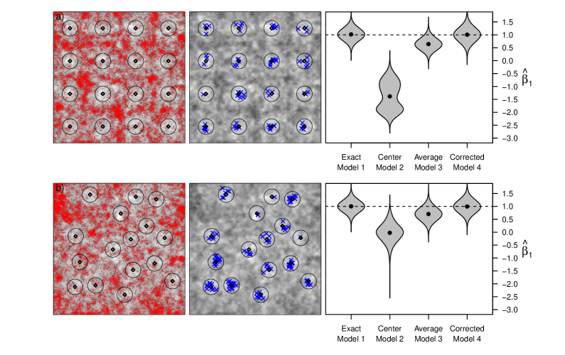
Figure 1:

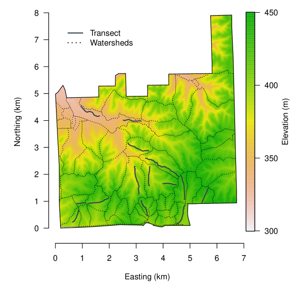
Figure 2:

Figure 3:

Table 1. Results of our simulation experiment that evaluated the influence of location uncertainty. For each scenario, we simulated 250 data sets and varied the sampling design by placing transect based on convenience or randomly (see Fig. 1 for illustration). We report the average number of detected individuals ($\bar{n}$) for each scenario. For each simulated data set, we fit four models which included: 1) Eq. 3 with the exact location of individuals known (model 1); 2) Eq. 3 using a surrogate predictor that was obtained from the center of the transect (model 2); 3) Eq. 3 with a surrogate predictor that was the transect average (model 3); and 4) Eq. 4 that does not require the exact location of the individuals to be known (model 4). We report the estimated coverage probability (CP) for the 95% confidence interval (CI) for the regression coefficient ($\beta_{1}$ in Eq. 1) estimated using each model. We calculated efficiency by dividing the average length of the 95% CI of $\hat{\beta}_{1}$ from the location uncertainty corrected model (model 4) by average length of the 95% CI of $\hat{\beta}_{1}$ estimated from Eq. 3 with the exact locations known (model 1).

Scenario	Transect	$\bar{n}$	CP (model 1)	CP (model 2)	CP (model 3)	CP (model 4)	Efficiency
1	Convenience	94	0.96	0.00	0.26	0.95	1.50
2	Random	124	0.93	0.00	0.38	0.98	1.49

Table 2. Parameter estimates and 95% confidence intervals (in parentheses) associated with the intercept ($\beta_{0}$) and regression coefficient $(\beta_{1})$ of the intensity function (Eq. 1) that determines the relationship between elevation and the abundance of Dickcissel (Fig. 3 a) at the Konza Prairie Biological Station. Also, reported is Akaike information criterion (AIC) values for four different models.

Model	Description	$\hat{\beta_{0}}$	$\hat{\beta_{1}}$	AIC
a	Eq. 3 (average elevation)	-9.13 (-9.44 -8.83)	0.033 (0.022, 0.044)	1405
b	Eq. 4 (exact distances)	-9.29 (-9.66, -8.93 )	0.042 (0.028, 0.056)	593
c	Eq. 7 (normal distance errors)	-9.29 (-9.66, -8.93)	0.042 (0.028, 0.056)	594
d	Eq. 7 (Laplace distance errors)	-9.29 (-9.66, -8.93)	0.042 (0.028, 0.056)	594

References

- Borchers et al. (2015) Borchers, D. L., Stevenson, B., Kidney, D., Thomas, L., and Marques, T. A. (2015). A unifying model for capture–recapture and distance sampling surveys of wildlife populations. Journal of the American Statistical Association, 110(509):195–204.
- Boyle (2018) Boyle, W. A. (2018). CBP01 Variable distance line-transect sampling of bird population numbers in different habitats on Konza Prairie. Environmental Data Initiative. https://doi.org/10.6073/pasta/053fe6a82e54394a70ff22b4794c0489. Accessed: 2019-1-25.
- Bradter et al. (2013) Bradter, U., Kunin, W. E., Altringham, J. D., Thom, T. J., and Benton, T. G. (2013). Identifying appropriate spatial scales of predictors in species distribution models with the random forest algorithm. Methods in Ecology and Evolution, 4(2):167–174.
- Briggs (2018) Briggs, J. M. (2018). GIS20 GIS coverages defining Konza elevations. http://lter.konza.ksu.edu/content/gis20-gis-coverages-defining-konza-elevations. Accessed: 2019-1-25.
- Brost et al. (2015) Brost, B. M., Hooten, M. B., Hanks, E. M., and Small, R. J. (2015). Animal movement constraints improve resource selection inference in the presence of telemetry error. Ecology, 96:2590–2597.
- Buckland et al. (2001) Buckland, S. T., Anderson, D., Burnham, K., Laake, J., Thomas, L., and Borchers, D. (2001). Introduction to Distance Sampling: Estimating Abundance of Biological Populations. Oxford University Press.
- Buckland et al. (2016) Buckland, S. T., Oedekoven, C. S., and Borchers, D. L. (2016). Model-based distance sampling. Journal of Agricultural, Biological, and Environmental Statistics, 21(1):58–75.
- Burnham et al. (1980) Burnham, K. P., Anderson, D. R., and Laake, J. L. (1980). Estimation of density from line transect sampling of biological populations. Wildlife Monographs, (72):3–202.
- Carroll et al. (2006) Carroll, R. J., Ruppert, D., Stefanski, L. A., and Crainiceanu, C. M. (2006). Measurement Error in Nonlinear Models: A Modern Perspective. CRC press.
- Chandler and Hepinstall-Cymerman (2016) Chandler, R. and Hepinstall-Cymerman, J. (2016). Estimating the spatial scales of landscape effects on abundance. Landscape Ecology, 31(6):1383–1394.
- Conn et al. (2018) Conn, P. B., Johnson, D. S., Williams, P. J., Melin, S. R., and Hooten, M. B. (2018). A guide to bayesian model checking for ecologists. Ecological Monographs, 88(4):526–542.
- Cressie (1993) Cressie, N. (1993). Statistics for Spatial Data. John Wiley & Sons.
- Cressie and Wikle (2011) Cressie, N. and Wikle, C. (2011). Statistics for Spatio-Temporal Data. Wiley.
- Elith and Leathwick (2009) Elith, J. and Leathwick, J. R. (2009). Species distribution models: ecological explanation and prediction across space and time. Annual Review of Ecology, Evolution, and Systematics, 40(1):677–697.
- Fletcher et al. (ress) Fletcher, R., Hefley, T., Robertson, E., Zuckerberg, B. McCleery, R., and Dorazio, R. (in press). A practical guide for combining data to model species distributions. Ecology.
- Foster et al. (2012) Foster, S. D., Shimadzu, H., and Darnell, R. (2012). Uncertainty in spatially predicted covariates: is it ignorable? Journal of the Royal Statistical Society: Series C (Applied Statistics), 61(4):637–652.
- Gelfand (2010) Gelfand, A. E. (2010). Misaligned spatial data: the change of support problem. In Handbook of Spatial Statistics, pages 514–536. CRC Press.
- Gelfand and Schliep (2018) Gelfand, A. E. and Schliep, E. M. (2018). Bayesian inference and computing for spatial point patterns. In NSF-CBMS Regional Conference Series in Probability and Statistics, volume 10, pages 1–125. Institute of Mathematical Statistics and American Statistical Association.
- Gerber et al. (2018) Gerber, B. D., Hooten, M. B., Peck, C. P., Rice, M. B., Gammonley, J. H., Apa, A. D., and Davis, A. J. (2018). Accounting for location uncertainty in azimuthal telemetry data improves ecological inference. Movement Ecology, 6(1):14.
- Gotway and Young (2002) Gotway, C. A. and Young, L. J. (2002). Combining incompatible spatial data. Journal of the American Statistical Association, 97(458):632–648.
- Harris (1989) Harris, I. R. (1989). Predictive fit for natural exponential families. Biometrika, 76(4):675–684.
- Heaton (2011) Heaton, M. (2011). Kernel Averaged Predictors for Space and Space-time Processes. PhD thesis, Duke University.
- Heaton and Gelfand (2011) Heaton, M. J. and Gelfand, A. E. (2011). Spatial regression using kernel averaged predictors. Journal of Agricultural, Biological, and Environmental Statistics, 16(2):233–252.
- Heaton and Gelfand (2012) Heaton, M. J. and Gelfand, A. E. (2012). Kernel averaged predictors for spatio-temporal regression models. Spatial Statistics, 2:15–32.
- Hedley and Buckland (2004) Hedley, S. L. and Buckland, S. T. (2004). Spatial models for line transect sampling. Journal of Agricultural, Biological, and Environmental Statistics, 9(2):181–191.
- Hefley et al. (2014) Hefley, T. J., Baasch, D. M., Tyre, A. J., and Blankenship, E. E. (2014). Correction of location errors for presence-only species distribution models. Methods in Ecology and Evolution, 5(3):207–214.
- Hefley et al. (2019) Hefley, T. J., Boyle, W. A., and Mohankumar, N. M. (2019). Data for: Accounting for location uncertainty in distance sampling data. .
- Hefley et al. (2017) Hefley, T. J., Brost, B. M., and Hooten, M. B. (2017). Bias correction of bounded location errors in presence-only data. Methods in Ecology and Evolution, 8(11):1566–1573.
- Hefley and Hooten (2016) Hefley, T. J. and Hooten, M. B. (2016). Hierarchical species distribution models. Current Landscape Ecology Reports, 1(2):87–97.
- Hijmans et al. (2005) Hijmans, R. J., Cameron, S. E., Parra, J. L., Jones, P. G., and Jarvis, A. (2005). Very high resolution interpolated climate surfaces for global land areas. International Journal of Climatology, 25(15):1965–1978.
- Högmander (1991) Högmander, H. (1991). A random field approach to transect counts of wildlife populations. Biometrical Journal, 33(8):1013–1023.
- Hooten and Hefley (2019) Hooten, M. B. and Hefley, T. J. (2019). Bringing Bayesian Models to Life. CRC Press.
- Johnson et al. (2010) Johnson, D. S., Laake, J. L., and Ver Hoef, J. M. (2010). A model-based approach for making ecological inference from distance sampling data. Biometrics, 66(1):310–318.
- Kéry and Royle (2016) Kéry, M. and Royle, J. A. (2016). Applied Hierarchical Modeling in Ecology: Analysis of Distribution, Abundance and Species Richness in R and BUGS, volume 1: Prelude and Static Models. Academic Press.
- Knapp et al. (1998) Knapp, A. K., Briggs, J. M., Hartnett, D. C., and Collins, S. L. (1998). Grassland Dynamics: Long-Term Ecological Research in Tallgrass Prairie. Oxford University Press.
- Lele et al. (2010) Lele, S. R., Nadeem, K., and Schmuland, B. (2010). Estimability and likelihood inference for generalized linear mixed models using data cloning. Journal of the American Statistical Association, 105(492):1617–1625.
- Miguet et al. (2017) Miguet, P., Fahrig, L., and Lavigne, C. (2017). How to quantify a distance-dependent landscape effect on a biological response. Methods in Ecology and Evolution, 8(12):1717–1724.
- Miller et al. (2019) Miller, D. A., Pacifici, K., Sanderlin, J., and Reich, B. (2019). The recent past and promising future of data integration methods to estimate species’ distributions. Methods in Ecology and Evolution, 10(1):22–37.
- Miller et al. (2013) Miller, D. L., Burt, M. L., Rexstad, E. A., and Thomas, L. (2013). Spatial models for distance sampling data: recent developments and future directions. Methods in Ecology and Evolution, 4(11):1001–1010.
- Mitchell et al. (2017) Mitchell, P. J., Monk, J., and Laurenson, L. (2017). Sensitivity of fine-scale species distribution models to locational uncertainty in occurrence data across multiple sample sizes. Methods in Ecology and Evolution, 8(1):12–21.
- Montgomery et al. (2011) Montgomery, R. A., Roloff, G. J., and Ver Hoef, J. M. (2011). Implications of ignoring telemetry error on inference in wildlife resource use models. The Journal of Wildlife Management, 75(3):702–708.
- Nelder and Mead (1965) Nelder, J. A. and Mead, R. (1965). A simplex method for function minimization. The Computer Journal, 7(4):308–313.
- Pacifici et al. (ress) Pacifici, K., Reich, B., Miller, D., and Pease, B. (in press). Resolving misaligned spatial data with integrated distribution models. Ecology.
- Pawitan (2001) Pawitan, Y. (2001). In All Likelihood: Statistical Modelling and Inference Using Likelihood. Oxford University Press.
- R Core Team (2019) R Core Team (2019). R: A Language and Environment for Statistical Computing. R Foundation for Statistical Computing, Vienna, Austria.
- Robinson (1950) Robinson, W. S. (1950). Ecological correlations and the behavior of individuals. American Sociological Review, 15(3):351–357.
- Stoklosa et al. (2015) Stoklosa, J., Daly, C., Foster, S. D., Ashcroft, M. B., and Warton, D. I. (2015). A climate of uncertainty: accounting for error in climate variables for species distribution models. Methods in Ecology and Evolution, 6(4):412–423.
- Stoyan (1982) Stoyan, D. (1982). A remark on the line transect method. Biometrical Journal, 24(2):191–195.
- Stuber et al. (2017) Stuber, E. F., Gruber, L. F., and Fontaine, J. J. (2017). A Bayesian method for assessing multi-scale species-habitat relationships. Landscape Ecology, 32(12):2365–2381.
- Temple (2002) Temple, S. A. (2002). Dickcissel. In The Birds of North America Online. Cornell Lab of Ornithology, Ithaca, NY.
- Walker (2018) Walker, N. B. (2018). Bias Correction of Bounded Location Errors in Binary Data. Masters Report, Kansas State University.
- Walker et al. (sion) Walker, N. B., Hefley, T. J., and Walsh, D. P. (under revision). Bias correction of bounded location errors in binary data. Biometrics.
- Williams et al. (2017) Williams, P. J., Hooten, M. B., Womble, J. N., Esslinger, G. G., Bower, M. R., and Hefley, T. J. (2017). An integrated data model to estimate spatiotemporal occupancy, abundance, and colonization dynamics. Ecology, 98(2):328–336.
- Zimmerman (1993) Zimmerman, J. L. (1993). The Birds of Konza: The Avian Ecology of the Tallgrass Prairie. University Press of Kansas.