Running Head: Tree shrinkage priors
Model selection for ecological community data using tree shrinkage priors
Trevor J. Hefley
Department of Statistics
Kansas State University
Haoyu Zhang
Department of Statistics
Kansas State University
Brian R. Gray
U.S. Geological Survey
Upper Midwest Environmental Sciences Center
La Crosse, Wisconsin
brgray@usgs.gov
Kristen L. Bouska
U.S. Geological Survey
Upper Midwest Environmental Sciences Center
La Crosse, Wisconsin
kbouska@usgs.gov
Contribution type: Article
Word count: 304 (abstract); 10,763 (total)
Number of references: 72
Number of figures: 5
Number of tables: 1
Corresponding author:
Trevor J. Hefley
Department of Statistics
205 Dickens Hall
1116 Mid-Campus Drive North
Manhattan, KS 66506
(785)-532-0703
thefley@ksu.edu
Statement of authorship: T.J.H, B.R.G and K.L.B conceived
the study. T.J.H and H.Z developed the statistical methods and conducted
the data analysis. T.J.H and H.Z wrote the manuscript. All authors
contributed substantially to revisions.
Data accessibility statement: The aquatic vegetation and fisheries data are publicly available from U.S. Geological Survey (2019), but the specific subsets used in this study will be archived in the Dryad Digital Repository. For the purpose of peer review, the data have been submitted as supporting material as a compressed file named Data.zip.
Reproducibility statement: Annotated computer code capable
of reproducing all results and figures associated with the aquatic
vegetation and fisheries data examples are provided in Appendix S1
and S2.
Abstract
Researchers and managers model ecological communities to infer the biotic and abiotic variables that shape species’ ranges, habitat use, and co-occurrence which, in turn, are used to support management decisions and test ecological theories. Recently, species distribution models were developed for and applied to data from ecological communities. Model development and selection for ecological community data is difficult because a high level of complexity is desired and achieved by including numerous parameters, which can degrade predictive accuracy and be challenging to interpret and communicate. Like other statistical models, multi-species distribution models can be overparameterized. Regularization is a model selection technique that optimizes predictive accuracy by shrinking or eliminating model parameters. For Bayesian models, the prior distribution automatically regularizes parameters. We propose a tree shrinkage prior for Bayesian multi-species distributions models that performs regularization and reduces the number of regression coefficients associated with predictor variables. Using this prior, the number of regression coefficients in multi-species distributions models is reduced by estimation of unique regression coefficients for a smaller number of guilds rather than a larger number of species. We demonstrated our tree shrinkage prior using examples of presence-absence data for six species of aquatic vegetation and relative abundance data for 15 species of fish. Our results show that the tree shrinkage prior can increase the predictive accuracy of multi-species distribution models and enable researchers to infer the number and species composition of guilds from ecological community data. The desire to incorporate more detail and parameters into models must be tempered by the limitations of the data and objectives of a study, which may include developing models that have good predictive accuracy and output that is easier to share with policymakers. Our tree shrinkage prior reduces model complexity while incorporating ecological theory, expanding inference, and can increase the predictive accuracy and interpretability of Bayesian multi-species distribution models.
Key-words: Bayesian statistics, community ecology, ecological guild, joint species distribution model, model averaging, model selection, multi-species distribution model, prior distribution, regularization
Introduction
Over the past 20 years species distribution models (SDMs) have become one of the most widely used quantitative methods in ecology (Elith and Leathwick 2009; Franklin 2010; Guisan et al. 2017). Species distribution models are routinely fit to presence-only, presence-absence, and abundance data to understand the biotic and abiotic variables that influence the habitat use and geographic distribution of a species (Aarts et al. 2012; McDonald et al. 2013; Hefley and Hooten 2016). The output of SDMs are used in scientific studies to test ecological theories and in application to delineate areas of high conservation value which informs management decisions (e.g., Wisz et al. 2013; Guisan et al. 2013; Hefley et al. 2015). Regardless of the type of data or method, the ultimate goal when using SDMs includes making reliable inference and accurate predictions.
In many applications, a SDM is fit to data from a single species. If the study objectives require the analysis of data from multiple species, then a SDM is fit to data from each species and the models are combined using stacking (Norberg et al. in press ; Zurell et al. in press). Although this species-by-species approach is common it presents several challenges that limit the ability of researchers and managers to make reliable inference and accurate predictions (Hui et al. 2013; Madon et al. 2013; Taylor-Rodriguez et al. 2017). For example, if the goal of a study is to produce accurate range maps then spatial predictions for a species that is rare will lack precision. Imprecise spatial predictions result from parameter estimates that have a high variance, which occurs because parameters are estimated using limited data from only a single rare species (e.g., Hefley and Hooten 2015). As another example, consider the case where the goal is to infer the influence of a predictor variable such as temperature. Fitting a SDM for each species requires estimating a unique temperature coefficients for each species. Even if there are only a few predictor variables it will be difficult to summarize the regression coefficients for a moderate number of species, which will hinder communication with policymakers.
Recently, SDMs for multiple species have been developed. So-called joint- or multi-species distribution models (MSDMs) enable a single model to be fit simultaneously to data from multiple species; the benefits include: 1) community-level inference and resulting prediction; 2) incorporation of biotic interactions; 3) more accurate predictions of single-species’ distributions due to “borrowing of strength” across data from co-occurring species; and 4) the potential for model simplification.
Many types of MSDMs have been developed using statistical or machine learning approaches (see synthesis in Norberg et al. in press and Wilkinson et al. 2019). Hierarchical Bayesian modeling is a statistical approach that is easily customizable and widely used to model the distribution of multiple species (e.g., Taylor-Rodriguez et al. 2017; Johnson and Sinclair 2017; Lany et al. 2018; Schliep et al. 2018; Ovaskainen et al. 2017; Wilkinson et al. 2019). Briefly, hierarchical Bayesian models are specified using conditional probability distributions that represent the data collection process (i.e., the “data model”), the latent ecological process (i.e., the “process model”), and prior knowledge about parameters (i.e., the “parameter model”; Wikle et al. 2019, pgs. 11–13; Hobbs and Hooten 2015, ch. 6).
For presence-absence data, Wilkinson et al. (2019) describes the quintessential hierarchical Bayesian MSDM. This includes the data model
| (1) |
where if the site () is occupied by the species () and if absent, “Bern” is a Bernoulli distribution, is an inverse link function (e.g., logistic, probit), and is the latent process on the link scale. For MSDMs, a widely used process model is
| (2) |
where is a random vector with elements , is expected value (mean), and is the variance-covariance matrix of a multivariate normal distribution. The vector, , has elements and is typically specified using
| (3) |
where, for the species, is the intercept and are the regression coefficients (i.e., ). The vector contains measured predictor variables at the site, which are the same for all species (i.e., ). In Eq. 2, the process model is specified jointly (i.e., using a multivariate distribution) to enable sharing of information across species.
In previous studies, the variance-covariance matrix, in Eq. 2, accounted for residual autocorrelation due to space, time, and/or biotic interactions. For example, within the literature on MSDMs, a main focus of methodological developments has been on parametrizing to account for biotic factors, such as species co-occurrence, that can not be explained by the measured predictor variables (e.g., Warton 2008; Warton et al. 2015; Ovaskainen et al. 2017; Niku et al. 2017; Wilkinson et al. 2019). By comparison, however, there are only a few studies that have focused on the parameterization of in Eq. 2 (e.g., Johnson and Sinclair 2017).
Regardless of the type of data, most MSDMs use a linear equation to model the influence of predictor variables. For example, all seven methods compared by Wilkinson et al. (2019) use Eq. 3 which, if there are species and predictor variables, will result in regression coefficients. For even a small number of predictor variables and species, the overabundance of regression coefficients will be challenging to summarize and interpret and may result in a MSDM that is overparameterized.
For many Bayesian MSDMs, the parameter model or prior is specified using simple distributions. For example, in six of the seven methods presented by Wilkinson et al. (2019) priors for the regression coefficients were specified using uniform distributions or independent normal distributions with known hyperparameters (e.g., ). Although using simple parameter models is common practice, more sophisticated parameter models are useful. For example, the seventh method in Wilkinson et al. (2019) uses a multivariate normal distribution with unknown hyperparameters as a parameter model which enables estimation and inference regarding the correlation among regression coefficients. For MSDMs, the notion of a model for the parameters is important because it can enable novel inference and perform regularization. Regularization is a model selection technique used to optimize predictive accuracy by controlling model complexity (Bickel et al. 2006; Hooten and Hobbs 2015).
Johnson and Sinclair (2017) develop a hierarchical Bayesian MSDMs, which includes a parameter model that leverages the concept of ecological guilds (Simberloff and Dayan 1991). For MSDMs, the ecological guild concept is useful because it provides a framework to incorporate ecological theory and reduce the number of regression coefficients associated with predictor variables. For example, the ecological guild concept suggests that some species may respond to predictor variables in a similar direction and magnitude as a result of similar resource use or ecological role. In other words, species within the same guild may be associated with similar values of the regression coefficients in Eq. 3. If the regression coefficients for two or more species are effectively the same, then the complexity of the MSDM can be reduced by estimating unique regression coefficients for a smaller number of guilds rather than a larger number of species.
If the guild membership is known, then incorporating the guild concept into MSDMs is trivial and involves using Eq. 3 with a guild by predictor variable interaction effect rather than a species by predictor variable (Johnson and Sinclair 2017). In nearly all applications, the number and species compositions of the guilds is unknown and must be estimated from data which can be accomplished using model-based techniques. For example, as a heuristic imagine that the species-specific regression coefficients for a single predictor variable in Eq. 3 were known. In this example, the number and species composition of guilds could be determined by classifying or clustering the regression coefficients into homogeneous groups. The classification model would be easier to interpret when compared to the larger number of species-specific regression coefficients because it provides a data-driven approach to determine which species can be modeled with a single guild-level regression coefficient. This ad-hoc approach is a useful heuristic because it gives insight into how a large number of regression coefficients can be summarized using a model for the parameters. Within a hierarchical Bayesian framework, formalizing this concept is straightforward by specifying an appropriate parameter model.
Simple independent parameter models that are commonly used for MSDMs, such as , do not leverage the information in the data shared among species. The independence assumption eliminates the possibility that information about parameters will be shared across species. Shared information among the species, however, can be accessed by incorporating the guild concept into the parameter model. For example, Johnson and Sinclair (2017) developed a hierarchical Bayesian MSDM using a Dirichlet process mixture for the parameter model, which enables regression coefficients to be estimated using data from all species within the same guild. Briefly, the Dirichlet process mixture is a distribution that can be used as a parameter model to cluster the species into guilds while simultaneously fitting a MSDM to community data.
Classification and regression trees (CART; Breiman et al. 1984) are a machine learning approach with widespread use in ecology (De’ath and Fabricius 2000; De’ath 2002; Elith et al. 2008). For ecological data, CART offer a semi-automated approach to build predictive models that are easy to interpret. Although Bayesian variants of CART have been available for some time (e.g., Chipman et al. 1998; Denison et al. 1998), they are rarely used by ecologists. This is perhaps because accessible versions of Bayesian CART software are not easily modified to accommodate ecological data. For example, current implementations of Bayesian CART do not include a “data model,” which is needed to account for imperfect measurements of ecological processes. Conceptually, CART can be embedded within hierarchical Bayesian models (at any level), which would enable ecologists to exploit the benefit of both approaches (Shaby and Fink 2012).
In our work, we show how a specific type of CART can be used as a parameter model for Bayesian MSDMs. Similar to Johnson and Sinclair (2017), our approach leverages the concept of ecological guilds but reduces model complexity via a novel tree shrinkage prior (TSP). We illustrate the TSP by fitting MSDMs to presence-absence and relative abundance data collected to inform management of freshwater aquatic vegetation and fish populations. These data are collected as part of a long-term environmental monitoring program intended to inform management of the Upper Mississippi River System. Managers are required to use these data to make and justify management recommendations. This requires understanding the predictor variables that influence the distribution of a large number of species using models that can be easily shared with policymakers but that are capable of making accurate predictions.
Materials and methods
INCORPORATING GUILDS INTO MULTI-SPECIES DISTRIBUTION MODELS
The mechanics of incorporating guilds into hierarchical Bayesian MSDMs was presented by Johnson and Sinclair (2017). For MSDMs, this involves a simple modification of Eq. 3
| (4) |
where, is a vector that specifies the expected value for the process model at the site for species, contains intercept parameters for each species, and contains predictor variables measured at the site. The matrix has dimensions where the row contains an indicator variable that links the predictor variables to the guild-specific regression coefficients contained within the vector . The mathematical symbol denotes a Kronecker product. For example, let there be species, guilds, and predictor variables, then for the site, one configuration of Eq. 4 is
| (5) |
where the first and second species are members of the first guild and the third and fourth species are members of the second guild. The guild-specific regression coefficients are where the subscripts, , indicate the guild and the predictor variable.
Modifications to the example given in Eq. 5, illustrates that incorporating the guild concept into MSDM results in a model that is flexible and includes two special cases. For example, if is a matrix with all elements equal to one (i.e., ), then all species would be in a single guild. Similarly if is a identity matrix (i.e., a matrix with diagonal elements equal to one and zero on the off diagonal elements), then each species would be assigned to a unique guild; this results in the commonly used MSDM with unique species-specific regression coefficients (i.e., Eq. 3) and demonstrates that incorporating the guild concept into MSDMs can only improve the predictive accuracy.
If the number and species composition of the guilds was known, then the matrix would also be known. In practice, however, the number and species composition of the guilds are unknown, which requires estimation of . In turn, regularizes the MSDM because shrinks and reduces the number of regression coefficients from to .
TREE SHRINKAGE PRIOR
A general introduction to tree-based methods is given in James et al. (2013; ch. 8) while Linero (2017) provides a technical review of Bayesian tree approaches. We use vocabulary found in both James et al. (2013; ch. 8) and Linero (2017). The idea of a TSP is not new but, to our knowledge, has been used in only one unrelated setting (Guhaniyogi and Sanso in press). For MSDMs, the idea is simple; the species within terminal nodes of the tree represent the guilds and determines the matrix in Eq. 4. Each terminal node is associated with guild-level regression coefficients for the predictor variables. For example, in what follows, we use presence-absence data for six species of aquatic vegetation and a single predictor variable (water depth). An example of a binary tree is given in Fig. 1 and shows which species share the same numerical value of the regression coefficients for the predictor variable water depth. In this example, the standard MSDM results in six regression coefficients (i.e., one for each species). For the predictor variable water depth, a MSDM specified using the tree shown in Fig. 1 results in only three regression coefficients. Recall that there are intercept parameters for each species, as a result the binary tree in Fig. 1 reduces the number of parameters in the MSDM from 12 to 9.
There are a variety of techniques to construct tree priors discussed within the statistics and machine learning literature (Linero 2017). Most techniques rely on a tree generating stochastic process (Linero 2017). Binary trees, like the example in Fig. 1, are a type of stochastic branching process (Dobrow 2016, ch. 4). Specification of a tree generating stochastic process involves specifying probability distributions that generate a tree structure as a random variable. For example, a simple stochastic binary tree generating process for the six species of aquatic vegetation in Fig. 1 involves specifying a distribution that determines the splitting of parent nodes and a second distribution that determines the allocation of species to the child nodes (e.g., in Fig. 1 super guild 1 is a parent node with guilds 1 and 2 as child nodes). For the aquatic vegetation example, one way to specify a binary tree generating stochastic process would involve using a “splitting distribution” that determines if a parent node should be split into two child nodes. If a draw from the splitting distribution results in a value of one, the parent node is split and draws from a “assignment distribution” allocates the species within the parent node to one of the two child nodes. In practice, the assignment distribution is whereas the splitting distribution is , where the hyperparameter controls the model complexity by inducing a prior on the guilds. For example, if then a binary tree is generated with six terminal nodes (guilds) that contain only a single species; when a tree with no splits is generated and all six species are in the same guild. Finally, the terminal nodes of the MSDM with a TSP has guild-level regression coefficients, , which require the specification of priors. For tree-based methods, simple models like are commonly used, (Linero 2017), however, more complex models have been developed (e.g., Gramacy and Lee 2008).
In sum, specifying a stochastic tree generating process results in an implied prior on the tree structure. For example, a so-called non-informative prior could be constructed by specifying a tree generating stochastic process that generates all possible combinations of guilds with equal probability (e.g., Atkinson and Sack 1992). For the aquatic vegetation example such a prior would result in 63 unique guilds. For this example, the MSDM with the TSP could be implemented using Bayesian model averaging (Oliver and Hand 1995). Model averaging is a well-known technique among ecologists (e.g., Hobbs and Hooten 2015; Dormann et al. 2018), however, this would require fitting 63 models (i.e., a model for each unique guild). Although we could fit a MSDM with the TSP to the aquatic vegetation data using Bayesian model averaging, this approach would not work for a larger number of species. For example, the fisheries data used to illustrate the TSP contains 15 species which results in 32,767 unique guilds. Despite advances in computational statistics, implementation of tree-based methods using Bayesian model averaging is challenging because of the potential for a large number trees (Chipman et al. 2001; Hooten and Hobbs 2015; Hooten and Hefley 2019, ch. 15). In the next section, we describe alternative strategies for model fitting that may be less familiar among ecologists.
MODEL FITTING
Hierarchical Bayesian MSDMs can be fit to presence-absence, abundance, and presence-only data using a variety of algorithms. Markov chain Monte Carlo (MCMC) algorithms are a type of stochastic sampling approach routinely used by ecologists and implemented in standard software such as WinBugs, JAGS, and Stan (Hooten and Hefley 2019). As such, we demonstrate the TSP using MCMC.
Compared with other commonly used ecological models, MCMC based implementation of Bayesian trees usually requires highly specialized algorithms. As a result, an inability to easily construct efficient algorithms has likely slowed the adoption of Bayesian regression trees (Linero 2017). For example, Bayesian model averaging, used to fit Bayesian trees to data, requires specialized algorithms (e.g., Oliver and Hand 1995; Hernández et al. 2018). As mentioned, however, this may be computationally challenging or infeasible for the TSP when there is a large number of guilds. To increase computational efficiency, search algorithms have been used to identify higher probability tree structures, however, as noted by Chipman et al. (1998), the “procedure is a sophisticated heuristic for finding good models rather than a fully Bayesian analysis, which presently seems to be computationally infeasible.” Significant progress continues in the development of computationally efficient implementations of Bayesian trees (Linero 2017), however, fitting tree-based models to data requires matching the model to computational algorithms which can be challenging for non-experts.
An appealing implementation for ecologists is presenting by Shaby and Fink (2012). The Shaby and Fink (2012) approach enables off-the-shelf software for tree-based methods, such as those available in R, to be embedded within hierarchical Bayesian models. This is appealing to ecologists because it makes the TSP accessible by eliminating the need to develop custom software to implement the TSP. Briefly, the technique of Shaby and Fink (2012) is an approximate Gibbs sampler that enables machine learning algorithms to be embedded within hierarchical Bayesian models. In what follows we use a model-based recursive partitioning approach that is available in the R package “partykit” and implemented within the lmtree(...) function (Hothorn et al. 2006; Zeileis et al. 2008; Zeileis and Hothorn 2019). Model-based recursive partitioning estimates a binary tree and consequently and in Eq. 4. The approximate Gibbs sampler of Shaby and Fink (2012) is similar to an empirical Bayesian step within a Gibbs sampler because priors for a portion of the unknown model parameters are replaced with estimates (Casella 2001). As a result, when using the Shaby and Fink (2012) approach, there are no distributions or hyperparameters associated with the TSP that must be specified.
In what follows, we use standard MCMC algorithms for MSDMs, but employ the Shaby and Fink (2012) approach. Constructing the approximate Gibbs sampler using the Shaby and Fink (2012) approach for the aquatic vegetation data example is incredibly simple and requires only six lines of R code and the ability to sample univariate normal and truncated normal distributions (e.g., using the R functions rnorm(...) and rtruncnorm(...); see section 2.3 in Appendix S1). To assist readers implementing similar MSDMs with the TSP, we provide tutorials with the computational details, annotated computer code, and the necessary code to reproduce all results and figures related to the analysis for the aquatic vegetation data and fisheries data examples (see Appendix S1 and S2).
STATISTICAL INFERENCE
A benefit of Bayesian inference is that uncertainty regarding the structure of the binary tree, and therefore the number and species composition of the guilds, is automatically accounted for. Under the Bayesian paradigm, samples from the posterior distribution of the trees are obtained during the model fitting process. The posterior distribution of the trees can be summarized to infer characteristics of the guilds. For example, the species composition of the guilds with the highest probability (given the data) can be obtained from the posterior distribution of the trees.
In addition, posterior distributions of the species-level and guild-level regression coefficients can be sampled and summarized. The species-level regression coefficients, akin to in Eq. 3, are a derived quantity calculated using
| (6) |
where the superscript is the current MCMC sample, is vector of regression coefficients for the species, is a matrix that contains indicator variables linking the guild-level coefficients to the species. In the presence of guild membership uncertainty, the species-level regression coefficients result in a posterior distribution that is a mixture of the guild-level regression coefficients.
When using the TSP, the posterior distribution of the regression coefficients for a species are akin to the model averaged posterior distribution obtained from fitting and averaging multiple MSDMs with differing species composition and numbers of guilds to the data. Similarly the guild-level regression coefficients are akin to the regression coefficients obtained from a single MSDM using a fixed guild structure. We recommend using the species-level regression coefficients to make inference because, with a finite amount of data, the species composition of the guilds will always be uncertain. Inference using the guild-level regression coefficients is conditional (i.e., valid for a fixed number and species composition of the guilds) and does not fully account for uncertainty.
LONG-TERM RESOURCE MONITORING DATA
The Mississippi River is the second longest river in North America and flows a distance of 3,734 km. The Upper Mississippi River System includes approximately 2,100 km of the Mississippi River channel and drains a basin covering 490,000 that contains 30 million people. The Upper Mississippi River Restoration Program was authorized under the Water Resources Development Act of 1986 (Public Law 99-662 ). The U.S. Army Corps of Engineers provides guidance, has overall Program responsibility, and established a long term resource monitoring (LTRM) element that includes collecting biological and geophysical data. The LTRM element is implemented by the U.S. Geological Survey, Upper Midwest Environment Sciences Center, in cooperation with the five Upper Mississippi River System states of Illinois, Iowa, Minnesota, Missouri, and Wisconsin (U.S. Geological Survey 2019). The expressed goal of the LTRM element is to “support decision makers with the information and understanding needed to maintain the Upper Mississippi River System as a viable multiple-use large river ecosystem.” The biological data collected by LTRM contains a large number of species and exemplifies the need for interpretable MSDMs with results that are easy to communicate to policymakers. For example, data from 154 species, some of which are rare or endangered, have been collected by the LTRM element since 1993; inferences from these data provide context for management recommendations for these or collections of these species.
As part of LTRM element, data on aquatic vegetation and fish are collected at multiple sites within six study reaches of the Upper Mississippi River. To illustrate our method, we use aquatic vegetation and fisheries data from navigation pool 8 collected in 2015. Complete details of data collection procedures for the aquatic vegetation data and fisheries data are given by Yin et al. (2000) and Gutreuter et al. (1995) respectively.
EXAMPLE 1: PRESENCE-ABSENCE OF AQUATIC VEGETATION
Our objective for the first example is to illustrate the TSP using a simple MSDM. As such, this example was designed to demonstrate the proposed methods rather than to provide scientifically valid inference. As such, we use only a single predictor variable (water depth) and presence-absence absence data of six species of aquatic vegetation. At 450 unique sites, the presence or absence of a species was recorded. For our example, we use data for broadleaf arrowhead (Sagittaria latifolia), Canadian waterweed (Elodea canadensis), coontail (Ceratophyllum demersum), stiff arrowhead (Sagittaria rigida), white water lily (Nymphaea odorata), and wild celery (Vallisneria americana). This resulted in a total of 2,700 observations. For our analysis, we randomly selected 225 sites and used data from these for model fitting. We used data from the remaining 225 sites to test the predictive accuracy of the models.
For the aquatic vegetation data, we use the data model
| (7) |
where is the presence or absence of the six species at the site (. The parameter vector is mapped to a probability by applying the inverse probit link function, , to each element. The parameter vector is specified using Eq. 4, but is simplified due to the single predictor variable in this example
| (8) |
where is a vector that contains intercept parameters for each species and is the recorded water depth at the site. As in Eq. 4, the matrix has dimensions where the row contains an indicator variable that links the predictor variables to the guild-specific regression coefficients contained within the vector . For the intercept, we use the prior because this results in a uniform distribution when is transformed using the function . That is, using the prior results in .
We used a computationally efficient MCMC algorithm to fit the MSDM to the aquatic vegetation data. This MCMC algorithm relies on an auxiliary variable formulation of the binary regression model and has been used to fit MSDMs to presence-absence data (Albert and Chib 1993; Wilkinson et al. 2019; Hooten and Hefley 2019, pgs. 246–253). For each model fit, we use one chain and obtain 100,000 draws from the posterior distribution, but retain every sample to decrease storage requirements. Each model fit takes approximately 30 minutes using a desktop computer (see Appendix S1). We inspect the trace plot for each parameter to ensure that the Markov chain is sampling from the stationary distribution (i.e., the posterior distribution). We discard the first 500 samples and use the remaining 9,500 samples for inference.
The model-based recursive partitioning approach available in the R function lmtree(...) and used to implement the TSP requires the specification of a tuning parameter (hereafter alpha; see Appendix S1). This tuning parameter, alpha, must be between zero and one and controls the splitting of parent nodes. Similar to the tree generating stochastic process (see Section TREE SHRINKAGE PRIOR), when alpha the tree has terminal nodes (guilds) that contain only a single species. When alpha the tree does not split and all six species are in the same guild. One way to estimate the tree tuning parameter, alpha, is to find the value that results in the most accurate predictions (Hobbs and Hooten 2015). For this example, we illustrate two approaches by estimating the predictive accuracy of our models with scores that use either in-sample or out-of-sample data. For the out-of-sample score, we use data from the 225 sites that were not used to fit the model to calculate the log posterior predictive density (LPPD). For the in-sample score, we calculate the Watanabe-Akaike information criteria (WAIC). For comparison between scoring approaches, we report as we would expect this and WAIC to result in similar numerical values (Gelman et al. 2014).
For Bayesian models, computing in-sample scores like WAIC require a measurement of a model’s complexity. In non-hierarchical non-Bayesian contexts, a model’s complexity is the number of parameters in the model. For example, using the MSDM applied to the aquatic vegetation data, the number of parameters ranges from 7 (i.e., six intercept parameters and one regression coefficient) to 12 (i.e., six intercept parameters and six regression coefficients). Measuring the complexity of our Bayesian MSDM with the TSP is more complicated than simply counting the number of parameters because of the shrinkage effect and because it is not obvious how many parameters are required to estimate the number and species composition of the guilds. Fortunately, when calculating Bayesian information criterion like WAIC, measure of model complexity such as the “effective number of parameters” are available without any additional effort. To understanding how the TSP controls the complexity of the MSDM, we report the effective number of parameters using Eq. 12 from Gelman et al. (2014) as alpha varies from zero to one.
EXAMPLE 2: FISH ABUNDANCE
Our objective for the second example is to demonstrate a different and complex data type that necessitates a more sophisticated use of the TSP and deeper ecological interpretation, similar to what ecologists may encounter in practice. Here we use relative abundance data from 15 species of fish that were sampled at 83 sites, which included several species that were present at only a small number of sites and are considered rare or species of concern (Table 1). For example, at 79 of the 83 sites (95%), a count of zero was recorded for river redhorse (Moxostoma carinatum; Table 1). At each site, numerous predictor variables were measured, but for our analysis we use water temperature, speed, and depth as these were most relevant to management of the Upper Mississippi River System.
The fisheries data were collected over three time periods which included period 1 (June 15 – July 31), period 2 (August 1 – September 14), and period 3 (September 15 – October 31). The time periods are hypothesized to correspond to changes in habitat use. For example, one hypothesis is that species composition of the guilds and the regression coefficient estimates associated with water temperature, speed, and depth may be different during each period. In what follows, we demonstrate how to incorporate such dynamics into MSDMs using the fisheries data.
For relative abundance data, Johnson and Sinclair (2017) discuss several commonly used MSDMs including a data model that has a marginal distribution of
| (9) |
where “ZIP” stands for zero-inflated Poisson, is the expected value of the Poisson mixture component, and is the mixture probability (Hooten and Hefley 2019; pg. 320). We specify the process model using Eq. 2 with and
| (10) |
where the guild composition and regression coefficients vary over the three sample periods as indicated by subscript such that and corresponds to period 1 (), period 2 (), or period 3 (). The vector are the three predictor variables (water temperature, speed and depth) measured at the site. In total, there are unique regression coefficients if the guilds contained only a single species for all three periods, which would also be the case if the standard MSDM (i.e., Eq. 3) with simple priors for the regression coefficients was used. For the mixture probability, process model variance, and intercepts we used the priors , , and respectively.
For each model fit, we use one chain and obtain 30,000 draws from the posterior distribution, but retain every sample to decrease storage requirements. We inspect the trace plot for each parameter to ensure the Markov chain is sampling from the stationary distribution. We discard the first 500 samples and use the remaining 2,500 samples for inference.
The computational cost to implement the TSP will increase as the number of species increase. In addition, allowing the number and species composition of the guilds to vary over the three periods increases the computational burden because the MSDM requires three TSPs instead of one. As a results, we do not select the value of the tree tuning parameter parameters that produces the best predictive model because fitting the MSDM once to the fisheries data takes about 23 hours using a desktop computer (see Appendix S2). Instead we choose a value of the tree tuning parameters that favors a small number of guilds, which we anticipate will make our results easier to share with policymakers. Similar to the aquatic vegetation example, the tree tuning parameters could be chosen to optimize the predictive ability of the model but this would make the annotated computer code provided in Appendix S2 difficult for many readers to use without access to high-performance computing resources.
Results
EXAMPLE 1: PRESENCE-ABSENCE OF AQUATIC VEGETATION
The value of the tree tuning parameter that produces the most accurate predictions was 0.6 when scored using LPPD and 0.025 when scored using WAIC. In what follows, we present results obtained from the MSDM with the TSP that used a value of the tree tuning parameter of 0.025 because this value was optimal based on WAIC, results in only a slight reduction in predictive accuracy when scored using LPPD, and yields a relatively large reduction in the number of parameters which simplifies statistical inference (Fig. 2). For the six species of aquatic vegetation, the posterior distributions for the species-level regression coefficient, obtained from Eq. 6, shows that the presence of wild celery has no statistical relationship with water depth while the remaining five species of vegetation exhibit a strong negative response to increases in water depth (Fig. 3a,b). In addition to the posterior distribution for the regression coefficients, derived quantities from the posterior distribution of the tree can provide insightful inference. For example, Fig 3c shows the posterior distribution of the number of terminal nodes (i.e., guilds) and Fig 3d shows the expected value of the posterior distribution of species co-occurrence within the same guild, both of which were derived from the posterior distribution of the trees. As another example, summaries of the posterior distribution of the tree may be of interest. For example, Fig. 3e shows the most likely tree, which is obtained from the mode of the posterior distribution of the trees and can be used to infer which guild structure is most likely. For the most likely tree, figure 3f shows the posterior distribution of the two guild-level regression coefficients. Again, caution must be taken when making inference from the guild-level regression coefficients because these are conditional on a single tree and do not account for guild uncertainty. For the aquatic vegetation data, however, the inference does not differ among the species-level and guild-level regression coefficients because the uncertainty in the number and species composition of the guilds is relatively low.
EXAMPLE 2: FISH ABUNDANCE
Similar to the aquatic vegetation example, we show the posterior distribution of the number of guilds (Fig. 4a,b,c), the expected value of species co-occurrence within the same guild (Fig. 4d,e,f), and the posterior distribution of the regression coefficients for each species (Figs. 5 and S1). During period 1, our results indicate that there are most likely two guilds (Fig 4a). The posterior distributions of the regression coefficients show that eight species (bluegill, bullhead minnow, emerald shiner, largemouth bass, mud darter, pugnose minnow, tadpole madtom, and weed shiner; hereafter “guild 1 during/in period 1”) have large decreases in relative abundance when water temperature and depth increases (Figs. 5 and S1). These results suggest guild 1 during period 1 is more abundant in shallower side channels and off-channel habitats compared to the main channel, where depth is maintained at a minimum of 2.75 m for navigation. Of the species in guild 1 during period 1 many are nest spawners (e.g., bluegill, bullhead minnow, largemouth bass, pugnose minnow, tadpole madtom) and our results correspond with habitat requirements for successful reproduction. During period 1, the remaining seven species (golden redhorse, longnose gar, river redhorse, river shiner, shorthead redhorse, smallmouth bass, spotfin shiner; hereafter “guild 2 during/in period 1”) have posterior distributions of the regression coefficients that indicate slight decrease in relative abundance when water temperature or depth increases, however, here is a non-negligible probability that these responses could be close to zero or even positive (Figs. 5 and S1). This suggest that during period 1 species in guild 2 are found over a broader range of conditions when compared to species in guild 1. Many of these species are classified as fluvial dependent or fluvial specialists, which are either generally found in lotic environments or require flowing water for some part of their life history (Galat and Zweimüller 2001; O’Hara et al. 2007).
During period 2, our results indicate that there is most likely a single guild that contains all 15 species of fish (Fig 4b). The posterior distributions of regression coefficients for all species generally have an expected value near zero, suggesting random associations with water depth, speed, and temperature (Fig. 5 and S1). The lack of a response to water depth, speed, and temperature during period 2 may be a result of active foraging in which species are moving in search of food.
During period 3, our results indicate that there are most likely two guilds (Fig 4c). The posterior distributions of the regression coefficients associated with depth indicate a negative response for five species (bluegill, largemouth bass, pugnose minnow, tadpole madtom, weed shiner; hereafter “guild 1 during/in period 3”), which suggests an avoidance of the main channel (Figs. 5 and S1). In addition, our results show a negative response to water speed for the species in guild 1 during period 3 which suggest associations with lentic habitats such as backwater lakes. As temperatures decrease during period 3 (September 15 – October 31), many of the species in guild 1 are known to move into slow-moving backwaters to minimize energy expenditures during winter conditions. During period 3, six species (bullhead minnow, emerald shiner, river redhorse, shorthead redhorse, smallmouth bass, spotfin shiner; “guild 2 during/in period 3”) had a slightly positive association with water speed and negative association with water temperature (Figs. 5 and S1). These results suggest that species in guild 2 during period 3 are more likely to inhabit the main channel and side channels during this period than off-channel habitats. During period 3, there are four species (golden redhorse, longnose gar, mud darter, and river shiner) whose posterior distributions of regression coefficients do not clearly delineate guild association. These results suggest either a high level of guild uncertainty, insufficient data, or weaker associations with the variables examined.
In summary, the number and composition of guilds changed over the three periods, suggesting shifts in habitat associations and species interactions through time. Whether these shifts were related to specific requirements for spawning, foraging, or overwintering would require additional field research designed to answer such questions, but our results are consistent with our understanding of fluvial dependence and general habitat guilds.
Discussion
A benefit of hierarchical Bayesian modeling is that statistical models can be easily customized to match the goals of a study. In what follows, we discuss modifications to the data and/or process models that have been commonly used to accommodate different types and quality of data. The modifications we discuss can be incorporated without making major changes to the basic framework we presented. We begin by discussing modifications to the data model. For our aquatic vegetation and fisheries data examples we used data models that were appropriate for presence-absence and relative abundance data, respectively. Other types of ecological data may require the specification of different distributions for the data. For example, a beta distribution is often used for plant cover data, which are usually reported as percentages (Wright et al. 2017; Damgaard and Irvine in press). Our approach, using the process model in Eq. 3 and TSP, could be used to develop a MSDM for plant cover data by specifying a beta distribution as the data model. Similarly, selecting a data model that matches key characteristics of the observed data (e.g., the support) is a common model building practice and applications using the TSP are straightforward (Hobbs and Hooten 2015; Hooten and Hefley 2019).
Many types of ecological data are measured with error. For example, presence-absence data may contain false-negatives (Tyre et al. 2003; Martin et al. 2005; Gray et al. 2013). For MSDMs, accounting for measurement error in the data is an important component of the model building process (Beissinger et al. 2016; Warton et al. 2016; Tobler et al. 2019). For example, multi-species occupancy models have been developed to account for false-negatives in presence-absence community data (Dorazio and Royle 2005). Model selection is challenging for multi-species occupancy models (Broms et al. 2016), however, using the approaches demonstrated in this paper, it is straightforward to implement the TSP for the multi-species occupancy model. This would involve adding a fourth level to the hierarchical MSDM in Eqs. 2–3 that accounts for the possibility of false-negatives in the presence-absence data (Hooten and Hefley 2019, ch. 23). Using the information provided in Appendix S1 in concert with Dorazio and Rodriguez (2012) or Hooten and Hefley (2019; ch. 23) would yield an efficient implementation that requires a minimal amount of additional programming.
As noted in the introduction, a main focus of methodological development within the literature on MSDMs has been on parametrizing the variance-covariance matrix, , for the process model in Eq. 2. In previous studies the variance-covariance matrix was specified to account for residual autocorrelation due to space, time, or biotic interactions. These modifications to the variance-covariance matrix can be incorporated into a MSDM that uses the TSP. For example, latent variables parameterizations have been used to induce dependence among species and estimate (Walker and Jackson 2011; Warton et al. 2015; Hui 2016). As another example, Johnson and Sinclair (2017) note that spatial or temporal autocorrelation can be accounted for by including basis functions to estimate (Hefley et al. 2017). In both the latent variables parameterization and basis function approach, the matrix is implicitly specified using a “random effects” or “first-order representation” (Hefley et al. 2017; Wikle et al. 2019, pgs. 156–157).
The TSP is easy to program using the approximate Gibbs sampling approach from Shaby and Fink (2012) and requires only a few additional lines of code when compared to Bayesian MSDMs that use simple priors. The computational burden to implement the TSP, however, is considerably larger which may increase the run-time required to fit MSDMs to data. For example, fitting independent models for single-species or MSDM with simple priors to data is faster because the number and species composition of the guilds does not have to be estimate and it may be easy to parallelize the computational procedure (Hooten and Hefley 2019, ch. 19; Hooten et al. in press). In general, the TSP will become more computationally challenging to implement as the number of species increases. For example, our implementation which uses a model-based recursive partitioning approach available in the R function lmtree(...) has a computational complexity that increase nonlinearly with the number of species. As a result fitting a MSDM to data for a small number of species is relatively fast as demonstrated by our example with six species of aquatic vegetation, however, model fitting requires much more time for a larger number of species as demonstrated by our example with 15 species of fish. The increase in computational time is caused by the increase in the number of possible guilds. Based on our experience and using the computational approaches presented in this paper, the TSP becomes infeasible to fit to data that contains more than roughly twenty species, however, feasibility will vary by data set and computer resources. Although this is a current limitation of the TSP, other Bayesian MSDMs that incorporate the guild concept face similar challenges (e.g., Johnson and Sinclair 2017) which demonstrates the need for more efficient algorithms for “big” ecological communities.
Currently we suggest two approaches to alleviate the computational burden when applying our approach to a large number of species. The first suggestion is to choose off-the-shelf tree methods that use multiple processors (or cores). For example, we used the R function lmtree(...)which allows users to choose the number of processor cores for tree related computations. In practice, implementation that exploits multiple processors should reduce the time required to fit a MSDM with the TSP to data, however, gains will vary by application. The second approach to reduce the computational burden involves using values of the tree hyperparameters that favor a small number of guilds. In studies with a large number of species, choosing a value of the tree hyperparameters that results in a small number of guilds may reduce the predictive accuracy of the model, however, model fitting will likely be quicker. In addition a small number of guilds may be desirable for studies that contain a large number of species because interpretation of the results for a larger number of guilds may be challenging. Both techniques, using multiple cores and reducing the number of guilds, were illustrated in our fisheries data example (see Appendix S2). As with most computationally demanding statistical methods, advances may soon obviate the current challenges.
Model development, implementation, and selection for data from ecological communities is difficult because a high level of complexity is desired which can be achieved by including numerous parameters. For example, commonly used MSDMs are specified so that each species has a unique regression coefficient for each predictor variable (e.g., Wilkinson et al. 2019). As a result it is common practice to overparameterize MSDMs, which can degrade predictive accuracy and produce results that are difficult to interpret and communicate. We illustrated how to reduce the number of parameters in commonly used Bayesian MSDMs by replacing simple prior distributions for regression coefficients with a TSP. The TSP reduces model complexity while incorporating ecological theory, expanding inference, and can increase the predictive accuracy and interpretability of Bayesian MSDMs.
Acknowledgements
The U.S. Army Corps of Engineers’ Upper Mississippi River Restoration Program LTRM element is implemented by the U.S. Geological Survey, Upper Midwest Environment Sciences Center, in cooperation with the five Upper Mississippi River System states of Illinois, Iowa, Minnesota, Missouri, and Wisconsin. The U.S. Army Corps of Engineers provides guidance and has overall Program responsibility. The authors acknowledge support for this research from USGS G17AC00289. Use of trade, product, or firm names does not imply endorsement by the U.S. Government.
Data accessibility
The aquatic vegetation and fisheries data are publicly available from U.S. Geological Survey (2019), but the specific subsets used in this study will be archived in the Dryad Digital Repository. For the purpose of peer review, the data have been submitted as supporting material as a compressed file labeled Data.zip.
References
- Aarts et al. (2012) Aarts, G., Fieberg, J., and Matthiopoulos, J. (2012). Comparative interpretation of count, presence–absence and point methods for species distribution models. Methods in Ecology and Evolution, 3(1):177–187.
- Albert and Chib (1993) Albert, J. H. and Chib, S. (1993). Bayesian analysis of binary and polychotomous response data. Journal of the American Statistical Association, 88(422):669–679.
- Atkinson and Sack (1992) Atkinson, M. D. and Sack, J.-R. (1992). Generating binary trees at random. Information Processing Letters, 41(1):21–23.
- Beissinger et al. (2016) Beissinger, S. R., Iknayan, K. J., Guillera-Arroita, G., and Zipkin, E. F. e. a. (2016). Incorporating imperfect detection into joint models of communities: A response to Warton et al. Trends in Ecology & Evolution, 31(10):736–737.
- Bickel et al. (2006) Bickel, P. J., Li, B., Tsybakov, A. B., van de Geer, S. A., Yu, B., Valdés, T., Rivero, C., Fan, J., and van der Vaart, A. (2006). Regularization in statistics. Test, 15(2):271–344.
- Breiman et al. (1984) Breiman, L., Friedman, J. H., Olshen, R. A., and Stone, C. J. (1984). Classification and Regression Trees. Wadsworth and Brooks.
- Broms et al. (2016) Broms, K. M., Hooten, M. B., and Fitzpatrick, R. M. (2016). Model selection and assessment for multi-species occupancy models. Ecology, 97(7):1759–1770.
- Casella (2001) Casella, G. (2001). Empirical Bayes Gibbs sampling. Biostatistics, 2(4):485–500.
- Chipman et al. (2001) Chipman, H., George, E. I., and McCulloch, R. E. (2001). The practical implementation of Bayesian model selection. IMS Lecture Notes - Monograph Series, pages 65–134.
- Chipman et al. (1998) Chipman, H. A., George, E. I., and McCulloch, R. E. (1998). Bayesian CART model search. Journal of the American Statistical Association, 93(443):935–948.
- Damgaard and Irvine (ress) Damgaard, C. F. and Irvine, K. M. (in press). Using the beta distribution to analyse plant cover data. Journal of Ecology.
- De’ath (2002) De’ath, G. (2002). Multivariate regression trees: a new technique for modeling species–environment relationships. Ecology, 83(4):1105–1117.
- De’ath and Fabricius (2000) De’ath, G. and Fabricius, K. E. (2000). Classification and regression trees: a powerful yet simple technique for ecological data analysis. Ecology, 81(11):3178–3192.
- Denison et al. (1998) Denison, D. G., Mallick, B. K., and Smith, A. F. (1998). A Bayesian CART algorithm. Biometrika, 85(2):363–377.
- Dobrow (2016) Dobrow, R. P. (2016). Introduction to Stochastic Processes with R. John Wiley & Sons.
- Dorazio and Rodriguez (2012) Dorazio, R. M. and Rodriguez, D. T. (2012). A Gibbs sampler for Bayesian analysis of site-occupancy data. Methods in Ecology and Evolution, 3(6):1093–1098.
- Dorazio and Royle (2005) Dorazio, R. M. and Royle, J. A. (2005). Estimating size and composition of biological communities by modeling the occurrence of species. Journal of the American Statistical Association, 100(470):389–398.
- Dormann, C., Calabrese, J., Guillera-Arroita, G. and Matechou, E. and Bahn, V., Bartoń, K., Beale, C. et al. (2018) Dormann, C., Calabrese, J., Guillera-Arroita, G. and Matechou, E. and Bahn, V., Bartoń, K., Beale, C. et al. (2018). Model averaging in ecology: a review of Bayesian, information-theoretic, and tactical approaches for predictive inference. Ecological Monographs, 88(4):485–504.
- Elith and Leathwick (2009) Elith, J. and Leathwick, J. R. (2009). Species distribution models: ecological explanation and prediction across space and time. Annual Review of Ecology, Evolution, and Systematics, 40(1):677–697.
- Elith et al. (2008) Elith, J., Leathwick, J. R., and Hastie, T. (2008). A working guide to boosted regression trees. Journal of Animal Ecology, 77(4):802–813.
- Franklin (2010) Franklin, J. (2010). Mapping Species Distributions: Spatial Inference and Prediction. Cambridge University Press.
- Galat and Zweimüller (2001) Galat, D. L. and Zweimüller, I. (2001). Conserving large-river fishes: is the highway analogy an appropriate paradigm? Journal of the North American Benthological Society, 20(2):266–279.
- Gelman et al. (2014) Gelman, A., Hwang, J., and Vehtari, A. (2014). Understanding predictive information criteria for bayesian models. Statistics and Computing, 24(6):997–1016.
- Gramacy and Lee (2008) Gramacy, R. B. and Lee, H. K. H. (2008). Bayesian treed Gaussian process models with an application to computer modeling. Journal of the American Statistical Association, 103(483):1119–1130.
- Gray et al. (2013) Gray, B. R., Holland, M. D., Yi, F., and Starcevich, L. A. H. (2013). Influences of availability on parameter estimates from site occupancy models with application to submersed aquatic vegetation. Natural Resource Modeling, 26(4):526–545.
- Guhaniyogi and Sanso (ress) Guhaniyogi, R. and Sanso, B. (in press). Large multi-scale spatial kriging using tree shrinkage priors. Statistica Sinica.
- Guisan et al. (2017) Guisan, A., Thuiller, W., and Zimmermann, N. E. (2017). Habitat Suitability and Distribution Models: With Applications in R. Cambridge University Press.
- Guisan et al. (2013) Guisan, A., Tingley, R., Baumgartner, J. B., Naujokaitis-Lewis, I., Sutcliffe, P. R., Tulloch, A. I., and et al. (2013). Predicting species distributions for conservation decisions. Ecology Letters, 16(12):1424–1435.
- Gutreuter et al. (1995) Gutreuter, S., Burkhardt, R., and Lubinski, K. (1995). Long Term Resource Monitoring Program Procedures: Fish Monitoring. https://umesc.usgs.gov/documents/reports/1995/95p00201.pdf. Accessed: 2019-6-20.
- Hefley et al. (2015) Hefley, T. J., Baasch, D. M., Tyre, A. J., and Blankenship, E. E. (2015). Use of opportunistic sightings and expert knowledge to predict and compare whooping crane stopover habitat. Conservation Biology, 29(5):1337–1346.
- Hefley et al. (2017) Hefley, T. J., Broms, K. M., Brost, B. M., Buderman, F. E., Kay, S. L., Scharf, H. R., Tipton, J. R., Williams, P. J., and Hooten, M. B. (2017). The basis function approach for modeling autocorrelation in ecological data. Ecology, 98(3):632–646.
- Hefley and Hooten (2015) Hefley, T. J. and Hooten, M. B. (2015). On the existence of maximum likelihood estimates for presence-only data. Methods in Ecology and Evolution, 6(6):648–655.
- Hefley and Hooten (2016) Hefley, T. J. and Hooten, M. B. (2016). Hierarchical species distribution models. Current Landscape Ecology Reports, 1(2):87–97.
- Hernández et al. (2018) Hernández, B., Raftery, A. E., Pennington, S. R., and Parnell, A. C. (2018). Bayesian additive regression trees using Bayesian model averaging. Statistics and Computing, 28(4):869–890.
- Hobbs and Hooten (2015) Hobbs, N. T. and Hooten, M. B. (2015). Bayesian Models: A Statistical Primer for Ecologists. Princeton University Press.
- Hooten and Hefley (2019) Hooten, M. B. and Hefley, T. J. (2019). Bringing Bayesian Models to Life. Chapman & Hall/CRC.
- Hooten and Hobbs (2015) Hooten, M. B. and Hobbs, N. T. (2015). A guide to Bayesian model selection for ecologists. Ecological Monographs, 85(1):3–28.
- Hooten et al. (ress) Hooten, M. B., Johnson, D. S., and Brost, B. M. (in press). Making recursive Bayesian inference accessible. The American Statistician.
- Hothorn et al. (2006) Hothorn, T., Hornik, K., and Zeileis, A. (2006). Unbiased recursive partitioning: a conditional inference framework. Journal of Computational and Graphical Statistics, 15(3):651–674.
- Hui (2016) Hui, F. K. (2016). boral–Bayesian ordination and regression analysis of multivariate abundance data in R. Methods in Ecology and Evolution, 7(6):744–750.
- Hui et al. (2013) Hui, F. K., Warton, D. I., Foster, S. D., and Dunstan, P. K. (2013). To mix or not to mix: comparing the predictive performance of mixture models vs. separate species distribution models. Ecology, 94(9):1913–1919.
- James et al. (2013) James, G., Witten, D., Hastie, T., and Tibshirani, R. (2013). An Introduction to Statistical Learning. Springer.
- Johnson and Sinclair (2017) Johnson, D. S. and Sinclair, E. H. (2017). Modeling joint abundance of multiple species using Dirichlet process mixtures. Environmetrics, 28(3):e2440.
- Lany et al. (2018) Lany, N. K., Zarnetske, P. L., Schliep, E. M., Schaeffer, R. N., Orians, C. M., Orwig, D. A., and Preisser, E. L. (2018). Asymmetric biotic interactions and abiotic niche differences revealed by a dynamic joint species distribution model. Ecology, 99(5):1018–1023.
- Linero (2017) Linero, A. R. (2017). A review of tree-based Bayesian methods. Communications for Statistical Applications and Methods, 24(6):543–559.
- Madon et al. (2013) Madon, B., Warton, D. I., and Araújo, M. B. (2013). Community-level vs species-specific approaches to model selection. Ecography, 36(12):1291–1298.
- Martin et al. (2005) Martin, T. G., Wintle, B. A., Rhodes, J. R., Kuhnert, P. M., Field, S. A., Low-Choy, S. J., Tyre, A. J., and Possingham, H. P. (2005). Zero tolerance ecology: improving ecological inference by modelling the source of zero observations. Ecology Letters, 8(11):1235–1246.
- McDonald et al. (2013) McDonald, L., Manly, B., Huettmann, F., and Thogmartin, W. (2013). Location-only and use-availability data: analysis methods converge. Journal of Animal Ecology, 82(6):1120–1124.
- Niku et al. (2017) Niku, J., Warton, D. I., Hui, F. K., and Taskinen, S. (2017). Generalized linear latent variable models for multivariate count and biomass data in ecology. Journal of Agricultural, Biological and Environmental Statistics, 22(4):498–522.
- Norberg, A., Abrego, N., Blanchet, F., Adler, F., Anderson, B. and Anttila, J., et al. (2019) Norberg, A., Abrego, N., Blanchet, F., Adler, F., Anderson, B. and Anttila, J., et al. (2019). A comprehensive evaluation of predictive performance of 33 species distribution models at species and community levels. Ecological Monographs, 89(3):e01370.
- O’Hara et al. (2007) O’Hara, M., Ickes, S., Gittinger, E., DeLain, S., Dukerschein, T., Pegg, M., and Kalas, J. (2007). Upper Mississippi River Restoration Program Long Term Resource Monitoring. U.S. Geological Survey, Upper Midwest Environmental Sciences Center, La Crosse, Wisconsin. LTRMP 2007-T001. https://umesc.usgs.gov/documents/reports/2007/2007-t001.pdf. Accessed: 2019-6-20.
- Oliver and Hand (1995) Oliver, J. J. and Hand, D. J. (1995). On pruning and averaging decision trees. In Machine Learning Proceedings 1995, pages 430–437. Elsevier.
- Ovaskainen et al. (2017) Ovaskainen, O., Tikhonov, G., Norberg, A., Guillaume Blanchet, F., Duan, L., Dunson, D., Roslin, T., and Abrego, N. (2017). How to make more out of community data? a conceptual framework and its implementation as models and software. Ecology Letters, 20(5):561–576.
- (54) Public Law 99-662. https://www.govinfo.gov/content/pkg/STATUTE-100/pdf/STATUTE-100-Pg4082.pdf. Accessed: 2019-6-30.
- Schliep et al. (2018) Schliep, E. M., Lany, N. K., Zarnetske, P. L., Schaeffer, R. N., Orians, C. M., Orwig, D. A., and Preisser, E. L. (2018). Joint species distribution modelling for spatio-temporal occurrence and ordinal abundance data. Global Ecology and Biogeography, 27(1):142–155.
- Shaby and Fink (2012) Shaby, B. A. and Fink, D. (2012). Embedding black-box regression techniques into hierarchical Bayesian models. Journal of Statistical Computation and Simulation, 82(12):1753–1766.
- Simberloff and Dayan (1991) Simberloff, D. and Dayan, T. (1991). The guild concept and the structure of ecological communities. Annual Review of Ecology and Systematics, 22(1):115–143.
- Taylor-Rodriguez et al. (2017) Taylor-Rodriguez, D., Kaufeld, K., Schliep, E. M., Clark, J. S., Gelfand, A. E., et al. (2017). Joint species distribution modeling: dimension reduction using Dirichlet processes. Bayesian Analysis, 12(4):939–967.
- Tobler et al. (2019) Tobler, M. W., Kéry, M., Hui, F. K., Guillera-Arroita, G., Knaus, P., and Sattler, T. (2019). Joint species distribution models with species correlations and imperfect detection. Ecology, 100(8):e02754.
- Tyre et al. (2003) Tyre, A. J., Tenhumberg, B., Field, S. A., Niejalke, D., Parris, K., and Possingham, H. P. (2003). Improving precision and reducing bias in biological surveys: estimating false-negative error rates. Ecological Applications, 13(6):1790–1801.
- U.S. Geological Survey (2019) U.S. Geological Survey (2019). Upper Mississippi River Restoration Program Long Term Resource Monitoring. https://umesc.usgs.gov/ltrm-home.html. Accessed: 2019-6-20.
- Walker and Jackson (2011) Walker, S. C. and Jackson, D. A. (2011). Random-effects ordination: describing and predicting multivariate correlations and co-occurrences. Ecological Monographs, 81(4):635–663.
- Warton (2008) Warton, D. I. (2008). Penalized normal likelihood and ridge regularization of correlation and covariance matrices. Journal of the American Statistical Association, 103(481):340–349.
- Warton et al. (2016) Warton, D. I., Blanchet, F. G., O’Hara, R., Ovaskainen, O., Taskinen, S., Walker, S. C., and Hui, F. K. (2016). Extending joint models in community ecology: A response to Beissinger et al. Trends in Ecology & Evolution, 31(10):737–738.
- Warton et al. (2015) Warton, D. I., Blanchet, F. G., O’Hara, R. B., Ovaskainen, O., Taskinen, S., Walker, S. C., and Hui, F. K. (2015). So many variables: joint modeling in community ecology. Trends in Ecology & Evolution, 30(12):766–779.
- Wikle et al. (2019) Wikle, C. K., Zammit-Mangion, A., and Cressie, N. (2019). Spatio-temporal Statistics with R. CRC Press.
- Wilkinson et al. (2019) Wilkinson, D. P., Golding, N., Guillera-Arroita, G., Tingley, R., and McCarthy, M. A. (2019). A comparison of joint species distribution models for presence–absence data. Methods in Ecology and Evolution, 10(2):198–211.
- Wisz, M., Pottier, J, Kissling, W., Pellissier, L., Lenoir, J., Damgaard, C. et al. (2013) Wisz, M., Pottier, J, Kissling, W., Pellissier, L., Lenoir, J., Damgaard, C. et al. (2013). The role of biotic interactions in shaping distributions and realised assemblages of species: implications for species distribution modelling. Biological Reviews, 88(1):15–30.
- Wright et al. (2017) Wright, W. J., Irvine, K. M., Warren, J. M., and Barnett, J. K. (2017). Statistical design and analysis for plant cover studies with multiple sources of observation errors. Methods in Ecology and Evolution, 8(12):1832–1841.
- Yin et al. (2000) Yin, Y., Langrehr, H., Shay, T., Cook, T., Cosgriff, R., Moore, M., and Petersen, J. (2000). Long Term Resource Monitoring Program Procedures: Aquatic Vegetation Monitoring. https://umesc.usgs.gov/documents/reports/ltrm_components/vegetation/95p00207.pdf. Accessed: 2019-6-20.
- Zeileis and Hothorn (2019) Zeileis, A. and Hothorn, T. (2019). Parties, models, mobsters: a new implementation of model-based recursive partitioning in R. https://cran.r-project.org/web/packages/partykit/vignettes/mob.pdf. Accessed: 2019-6-20.
- Zeileis et al. (2008) Zeileis, A., Hothorn, T., and Hornik, K. (2008). Model-based recursive partitioning. Journal of Computational and Graphical Statistics, 17(2):492–514.
- Zurell et al. (ress) Zurell, D., Zimmermann, N. E., Gross, H., Baltensweiler, A., Sattler, T., and Wüest, R. O. (in press). Testing species assemblage predictions from stacked and joint species distribution models. Journal of Biogeography.
Supporting Information
Additional Supporting Information may be found in the online version of this article.
Appendix S1
Tutorial with R code to reproduce the aquatic vegetation example and Figs. 2 and 3.
Appendix S2
Tutorial and R code to reproduce the fisheries example and Figs. 4, 5, and S1.
Appendix S3
Supporting Fig. S1.
Fig. 1. An example of a binary tree that is used to partition an ecological community that contains six species of aquatic vegetation into three guilds. The tree shrinkage prior uses a binary tree to determine which species share the same value of the regression coefficients, , for the predictor variable water depth. In this example, the standard priors for multi-species distribution model forces each species to have a unique regression coefficient. The binary tree identifies the species composition and number of guilds. For the species within a guild, a single regression coefficient is used to model the predictor variable water depth, which reduces the number of regression coefficients from six to three.
Fig. 2. Results from fitting multi-species distribution models to presence-absence data for six species of aquatic vegetation using the predictor variable water depth. Panel a shows how the predictive score, (where LPPD is the log posterior predictive density calculated from out-of-sample data), changes as the tree tuning parameter varies from zero to one. Panel b shows WAIC, which is similar to , but uses in-sample data. For both WAIC and , a lower score indicates more accurate predictions, which can be optimized by varying the tree tuning parameter from zero to one. Panel c shows the posterior mode of the number of guilds as the tree tuning parameter varies from zero to one while panel d shows the effective number of parameters. All models contain six species-specific intercept parameters, but the number of regression coefficients varies from one to six depending on the value of the tree tuning parameter. When the tree tuning parameter is set to one each species is assigned to a different guild, resulting in the standard species-specific MSDM (Eq. 3) with six regression coefficients for a total of 12 parameters. When the tree tuning parameter is set to zero the result is a single guild that contains all six species and one regression coefficient for a total of seven parameters. Panel e shows the expected value of the species-level regression coefficients associated with depth as the tree tuning parameter varies from zero to one. As the tree tuning parameter decreases to zero, the species-level regression coefficient estimates are shrunk towards , which is the regression coefficient estimate when all species are in the same guild.
Fig. 3. Posterior distributions and summaries obtained from fitting the multi-species distribution model to presence-absence data from 225 sites with a tree tuning parameter value of . Panel a shows the posterior distributions of the regression coefficient for all six species associated with the predictor variable water depth. Panel b shows the expected value of the probability of species presence as water depth varies from zero to three meters. Panel c shows the posterior distribution for the number of guilds. Panel d shows the expected value of the posterior distribution of species co-occurrence within the same guild. Panel e shows the mode of the posterior of the tree structure (i.e., the most probable guild structure). Panel f shows the posterior distributions of the regression coefficient for the two guilds from panel e. The color-coded tick marks on the horizontal axis of panels a and f are the expected value of the corresponding posterior distribution. The square-bracket notation is used to represent posterior density functions.
Fig. 4. Results obtained from fitting a multi-species distribution model to abundance data from 83 sites and 15 fish species. We specified the model to allow the number and species compositions of guilds to vary over three time periods. Panels a, b, and c show the posterior distribution for the number of guilds in time period 1 (June 15-July 31), period 2 (August 1- September 15), and period 3 (September 16 - October 31) respectively. Panels d, e, and f show the expected value of the posterior distribution of species co-occurrence within the same guild during periods 1, 2, and 3 respectively.
Fig. 5. Posterior distributions of regression coefficients obtained from fitting our multi-species distribution model to relative abundance data from 83 sites that included 15 species of fish (see Table 1 for species list). Panels a, b, and c show the posterior distributions of regression coefficients for the variables water temperature, speed, and depth for bluegill respectively, which was the most common species in our study. Panels d, e, and f show the posterior distributions of regression coefficients for the variables water temperature, speed, and depth for river redhorse respectively, which was the least common species in our study. The posterior distribution for river redhorse are bimodal due to uncertainty in the guild membership of the species. The color-coded tick marks on the horizontal axis shows the expected value of the corresponding posterior distribution. The square-bracket notation is used to represent posterior density functions. The predictor variables variables water temperature, speed, and depth were centered and standardized prior to fitting the model and had a standard deviation of 3.8, 0.16, and 0.44 respectively. Fig. S1 in Appendix S2 contains posterior distributions for all 15 species.
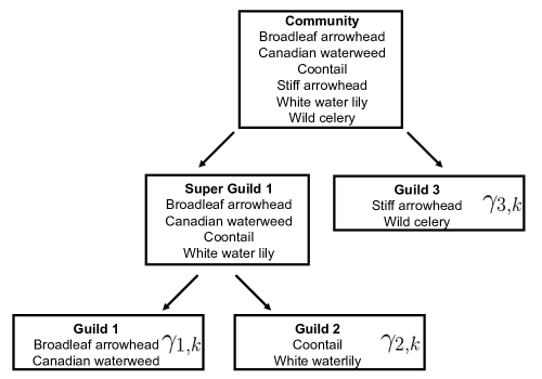
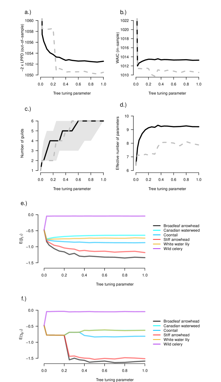
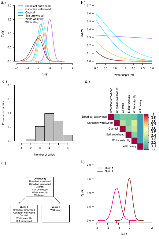
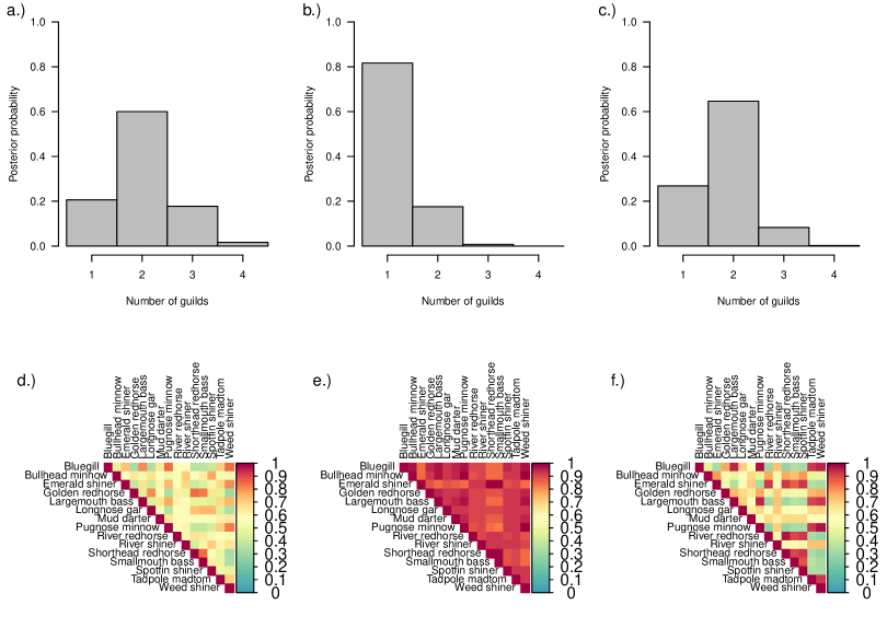
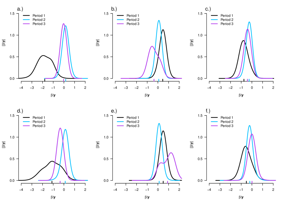
Table 1. Common name, species name, and percent of 83 sites with counts greater than zero for 15 species of fish used in our example.
| Common name | Species | Percent of sites with counts greater than zero |
|---|---|---|
| Bluegill | Lepomis macrochirus | 81% |
| Bullhead minnow | Pimephales vigilax | 45% |
| Emerald shiner | Notropis atherinoides | 48% |
| Golden redhorse | Moxostoma erythrurum | 53% |
| Largemouth bass | Micropterus salmoides | 84% |
| Longnose gar | Lepisosteus osseus | 22% |
| Mud darter | Etheostoma asprigene | 6% |
| Pugnose minnow | Opsopoeodus emiliae | 27% |
| River redhorse | Moxostoma carinatum | 5% |
| River shiner | Notropis blennius | 17% |
| Spotfin shiner | Cyprinella spiloptera | 71% |
| Shorthead redhorse | Moxostoma macrolepidotum | 62% |
| Smallmouth bass | Micropterus dolomieu | 49% |
| Tadpole madtom | Noturus gyrinus | 8% |
| Weed shiner | Notropis texanus | 54% |