Low-Cost Fiducial-based 6-Axis Force-Torque Sensor

Abstract

Commercial six-axis force-torque sensors suffer from being some combination of expensive, fragile, and hard-to-use. We propose a new fiducial-based design which addresses all three points. The sensor uses an inexpensive webcam and can be fabricated using a consumer-grade 3D printer. Open-source software is used to estimate the 3D pose of the fiducials on the sensor, which is then used to calculate the applied force-torque. A browser-based (installation free) interface demonstrates ease-of-use. The sensor is very light and can be dropped or thrown with little concern. We characterize our prototype in dynamic conditions under compound loading, finding a mean $R^{2}$ of over 0.99 for the $F_{x},F_{y},M_{x}$, and $M_{y}$ axes, and over 0.87 and 0.90 for the $F_{z}$ and $M_{z}$ axes respectively. The open source design files allow the sensor to be adapted for diverse applications ranging from robot fingers to human-computer interfaces, while the sdesign principle allows for quick changes with minimal technical expertise. This approach promises to bring six-axis force-torque sensing to new applications where the precision, cost, and fragility of traditional strain-gauge based sensors are not appropriate. The open-source sensor design can be viewed at http://sites.google.com/view/fiducialforcesensor.

I Introduction

I-A Motivation

Force-torque sensors are used extensively in both industry and research. We focus here on the use of these sensors in two examples: robotic grasping, where they are used to provide tactile feedback (e.g. detecting when contact is made), and in human computer interaction. However, commercial six-axis force-torque sensors can be both expensive and fragile. This combination makes them tricky to use for grasping, where controlled contact is desired, but a small coding error could easily smash and overload the sensor. One of the most common types of sensors, the ATI force/torque sensor, costs tens of thousands of dollars and relies on strain gauges that are fragile and have to be surrounded in a bulky package. For these reasons, we are motivated to consider new sensor designs that could promote the use of tactile data in the robotics community through being a combination of cheaper, easier to use, and more robust.

Figure 1: Consumer webcams and a printed fiducial markers can be used to create a six-axis force-torque sensor. We used four springs to build a platform free to move in all angular directions. We affixed two printed fiducials to the platform, and then aimed a consumer camera up at them. To the right, the camera view reveals the tag location. The tags are glued to the light shield, which is removable, allowing for easy design changes. Note that cardstock, which was removed for picture clarity, was used to diffuse the LED and avoid overexposing the camera. Green bottle cap is for scale.

I-B Related Work

Multiple designs have emerged recently taking advantage of the rich information available from consumer webcams. Even low-end webcams will output 640x480 RGB images at 15 frames-per-second (fps). The webcam-based sensors are particularly easy to manufacture and wire. Notable examples include the Gelsight [1], GelForce [2], TacTip [3], the Fingervision [4], and others. These sensors rely on cameras facing markers embedded in transparent or semi-transparent elastomer (often with supplemental LED lighting). These can be used to estimate shear, slip, and force, but tend not to do well in cases where the object hits the side of the finger instead of dead on. They also require casting elastomers.

Several MEMS multi-axis force-torque sensors have been developed, which use the same principle of creating a device free to deflect into multiple axes, but then measures them using capacitative [5] or piezoresistive [6] means. In [7] the deflection is measured using a camera as well, a CCD camera mounted to a microscope, however the device only measures two directions of force.

Prior work used MEMS barometers to create six-axis force-torque sensors with very low parts cost and good durability [8]. However, fabricating the sensor requires specialized lab equipment such as a degassing machine.

Other work explored estimating fingertip force via video, but only for human fingers [9, 10]. Commercial sensors like the Spacemouse and the OptoForce use similar ideas, but rely on custom circuitboards for a ranging sensor inside. In contrast, our work is straightforward to fabricate even for users unfamiliar with electronics.

I-C Contributions

In this paper, we investigate novel combinations of readily-accessible technologies to create six-axis force-torque sensors that are inexpensive, require minimal expertise to design and build, and are easily customized for diverse applications.

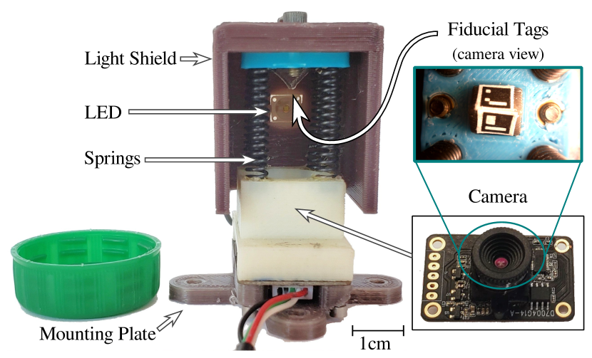
The proposed novel type of sensor makes six-axis force-torque measurements by tracking position and orientation displacement using the 3D pose estimate from fiducial tags, and uses a linear fit between displacement and applied force-torque. Fiducials are markers used to help locate objects or serve as points of reference. They can be found in robotics and augmented reality applications, where they usually take the form of printed paper markers glued onto various objects of interest. Sensors employing these fiducials operate by detecting the sharp gradients that are created between black and white pixels, such as one might find on a checkerboard. An example of two fiducials can be found in the top right of the labelled diagram of our sensor at Fig. 1. Using the known geometry of the tag (e.g. perpendicular sides of checkeboard), as well as known tag size and pre-determined camera calibration matrix, the 3D object pose (location and orientation) of the object can be estimated. This calculation is known as the solving the Perspective-n-Point (PnP) problem. We created prototypes utilizing two open-source tag protocols, AprilTags [11] and ArUco markers [12]; pictured in Fig. 1 are two ArUCo markers.

In the following sections, we begin with the design and fabrication process for our sensor. We follow with a theoretical analysis of how the sensor design parameters affect resolution, sensitivity, measurement range, and bandwidth. We also present an analysis of data collected from a prototype sensor. We conclude with a discussion of the advantages and limitations of this sensor.

II Design

II-A Sensor Design

Figure 2: The top row shows the viewpoint from the camera when different forces or torques are applied (the dotted grey line shows the center of the camera view). By tracking the movement of the fiducial(s), we can derive the force and torque exerted on the sensor.

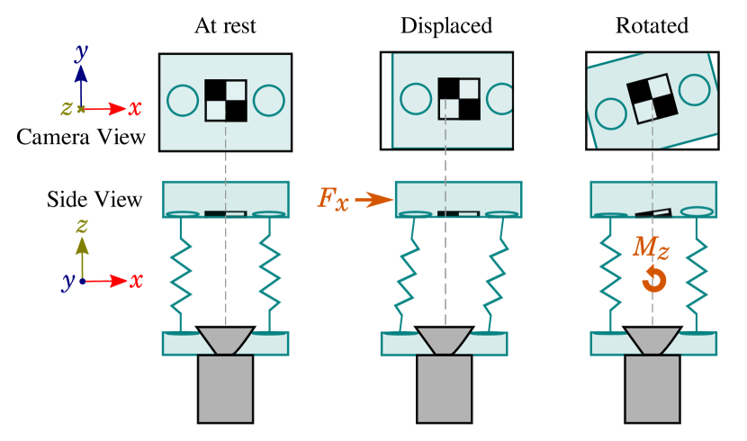
At a high level, the sensor consists of two main parts: a base and a platform above the base. The platform is connected to the base with 4 springs and can move in all directions with respect to the base. Two fiducial tags were glued to the underside of the platform. Then, a webcam pointed up at the tags was installed at the base. As force or torque is applied to the platform, the tags translate and rotate accordingly. The camera is used to track the 3D pose of the tags. Should there be a suitably linear relationship between the displacement and the force-torque applied, a short calibration procedure using known weights can be used to collect datapoints for regression. Given a known linear fit, the sensor can then output force and torque measurements. Fig. 2 shows the principle behind this fiducial-based force sensor.

II-B Design Goals

When designing the sensor prototype, a few considerations were made. First and foremost, the sensor needs to be sensitive to all six degrees of freedom (displacement in $x$, $y$, $z$ and rotation in yaw, pitch, roll). For illustrative purposes, the following analysis is performed in terms of specific specification values that are appropriate for a sample robot gripper. Alternate values for other use cases such as human-computer interfaces can be easily substituted. For grasping, between $\pm$ 40 N is realistic, and sensitivity of at least 1/10 N is desirable. Qualitatively, we want the sensor to be small (for grasping applications, the sensor should be roughly finger-sized), inexpensive, and robust. The sensor should allow for rapid prototyping and easy customization with minimal technical expertise. The sensor should be not only easy to fabricate, but also easy to use.

II-C Fabrication

Figure 3: Left, the four 3D printed parts are shown. Right, a diagram of the sensor as mounted to the commercial force sensor (in grey on the bottom) used in our experiments. The footprint of the sensor itself is the same as the camera circuitboard, 35.7 mm by 22.5 mm. The sensor height $h$ = 51 mm, while the camera lens is approximately $d_{tag}$ = 21 mm from the center of the tags. The light shield is offset on all three sides by $w_{gap}$ = 2.5 mm gap from the camera cover, and has width $w_{shield}$ = 31 mm. The fiducials are each $w_{tag}$ = 3.8 mm wide (or $4.5$ mm including the white border). The mounting plate attaches to mounting holes in the force sensor and has width $w_{bottom}$ = 45 mm.

II-C1 Physical Fabrication

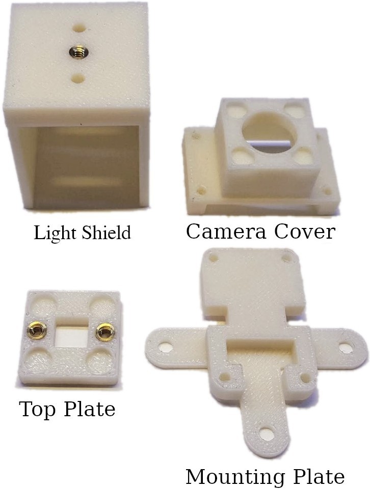
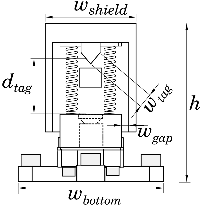
The four pieces in Fig. 3 (figure includes dimensions) are 3D-printed in two to three hours on an inexpensive consumer-grade device (Select Mini V2, Monoprice). Epoxy is used to glue the springs into the camera cover and top plate. The tags are printed on paper and glued in. A small piece of white cardstock is used to diffuse the LED (in the future, this would be built into the 3D design). Conveniently, the pose estimate is relative to the camera frame, and the sensor relies only on relative measurements, so the tag placement can be imprecise. The LED is mounted in and connected to a 3.3 V power source. The heat-set thread inserts (for bolting the light shield to the platform) are melted in with a soldering iron. The camera is placed between the mounting plate and camera cover and then everything is bolted together. The springs are steel compression springs available online as part of an assortment pack from Swordfish Tools. The spring dimensions are 2.54 cm long, 0.475 cm wide, and wire width of 0.071 cm, with a stiffness of approximately $0.7\text{\,}\mathrm{N}\mathrm{/}\mathrm{m}\mathrm{m}$. Fabrication can be completed in a day. The actual assembly, given a complete set of hardware and tools, can be completed in 30 minutes, depending on the epoxy setting time.

II-C2 Usage and Software

The only data cable used is the USB from the webcam to the computer. On the computer, the OpenCV Python library [13] (version 4.1.2) is used to detect the ArUco markers in the video feed. We used a commercial force-torque sensor to characterize our sensor, for which we used another freely available Python library (see [14]). The data from the commercial sensor (Model HEX-58-RE-400N, OptoForce, Budapest, Hungary) and the markers are read in parallel threads and timestamped, then recorded to CSV. Python is used for further analysis.

By using a consumer webcam, sensor reading is also possible without installing Python. To demonstrate this, we developed a simple interface using a Javascript ArUco tag detector library (see [15]). Fig. 4 shows a graphical user interface (GUI) that plots the $x$, $y$, and $z$-axes of the 3D pose estimate for a single tag.

Figure 4: Our prototype JavaScript-based interface (modified from the Js-aruco library example) [15]. In this way, sensor data can be read just by loading a webpage.

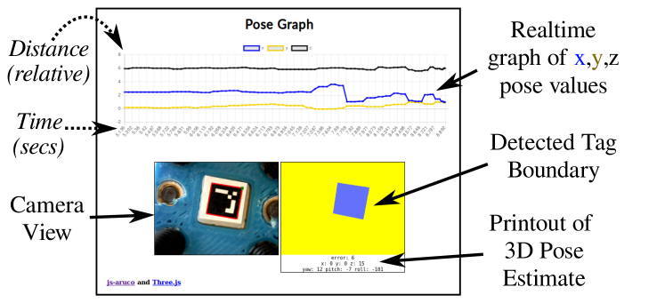
In theory, the sensor reading can be done on-the-go with a smartphone and a wireless or USB-C webcam (such as inexpensive endoscope inspection cameras found online).

II-C3 Calibration

Although we calibrated using a commercial force-torque sensor, the same can be achieved with a set of weights and careful clamping. The sensor can be clamped sideways to a sturdy surface to calibrate the $x$- and $y$-axes. A set of known weights is then attached to the center bolts on the light shield piece via a string. The same procedure can be applied to calibrate the $z$-axis, with the sensor clamping upside down to a tabletop. Finally, weights can be applied to the two side bolts to produce known torques while hanging upside down or sideways.

III Analysis

Considering the above design goals, there are a few primary concerns amenable to theoretical analysis: the sensor resolution, sensitivity, force range, and bandwidth. Here, sensor resolution is defined in bits (relative terms) and sensitivity in millimeters and degrees.

III-A Resolution

(a) A frame from the camera. $w_{frame}\times h_{frame}=640\times 480$ pixels, and $w_{img}\times h_{img}=150\times 240$ pixels.

(b) Side view. As per Fig. 3, $d_{tag}=21$ mm and $w_{tag}=4.5$ mm. Light orange indicates original tag position before displacement. Inset shows force applied.

Figure 5: Sensitivity calculation diagrams.

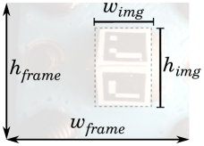
Let us conservatively estimate the discernible resolution of the tag system to be $d_{R}=1/4$ pixel, or $C=4$ counts per pixel. This factor exists because we have more than just binary information (1 bit) for every pixel. For instance, if a black/white intersection is halfway between two pixels, the pixels will be gray. (Tag algorithms also use the known grid geometry to achieve subpixel resolution – see the cornerSubPix function in the OpenCV library).

In that case, we can determine the resolution of the sensor itself geometrically, by looking at the number of pixels. The fact that the tags must stay on-screen limits the sensor resolution.

We can characterize an approximate $y$-axis resolution $r_{y}$ of the camera by taking the number of pixels available, multiplying by $C$, and converting our counts into bits.

$$r_{y} =\lfloor\log_{2}\left(C\cdot(h_{frame}-h_{img})\right)\rfloor+1$$ (1)

For instance, the calculations for our sensor prototype are as follows. In the $y$-axis,

$$r_{y} =\lfloor\log_{2}{\left(4\cdot(480-240)\right)}\rfloor$$ (2)

$$r_{y} =10~{}\text{bits}$$ (3)

In the $x$-axis, repeating the same calculations we have

$$r_{x} =\lfloor\log_{2}\left(C\cdot(w_{frame}-w_{img})\right)\rfloor+1$$ (4)

$$r_{x} =\lfloor\log_{2}{\left(4\cdot(640-150)\right)}\rfloor+1$$ (5)

$$r_{x} =11~{}\text{bits}$$ (6)

In the $z$-axis, our limitation is the same as the $y$-axis, so we have $r_{z}=11~{}\text{bits}$.

III-B Sensitivity

Let us now calculate the sensitivity of the sensor. We will start by looking at the minimum detectable travel in each of the $x$, $y$, and $z$-axes.

III-B1 Translational Sensitivity

In the $x$ and $y$ directions, we can measure the mm/px at rest (the sensor resolution varies a bit since the tag gets larger or smaller depending on the $z$ distance). Roughly, the tag measures $4.5\text{\,}\mathrm{m}\mathrm{m}$ and appears as $w_{tag}=150$ pixels in the image. Assuming as above that we can discern 4 counts per pixel, the theoretical sensitivity is

$$s_{y} =\frac{h_{frame}~{}$\text{\,}\mathrm{(}\mathrm{m}\mathrm{m}\mathrm{)}$}{h_{frame}~{}$\text{\,}\mathrm{(}\mathrm{p}\mathrm{x}\mathrm{)}$}d_{R}=\frac{4.5}{150}\cdot\frac{1}{4}=$0.0075\text{\,}\mathrm{m}\mathrm{m}$$$ (7)

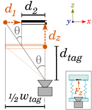
For the $z$-axis sensitivity, we consider that the tag will get smaller as it displaces in the $+z$ direction. Using a simple geometrical model (see Fig. 5(b)), given that the smallest detectable change in $xy$ plane is $1/4$ pixel, we can calculate what is the resulting change in $z$.

Using similar triangles, we see that

$$\frac{d_{1}}{d_{z}} =\frac{d_{2}}{d_{tag}}$$ (8)

$$d_{1}+d_{2} =w_{img}/2$$ (9)

$$d_{2} =(w_{img}/2)-d_{1}$$ (10)

We would like to work in $\text{\,}\mathrm{m}\mathrm{m}$, therefore we use the fact that the tag is 4.5 mm and appears as 150 px.

$$d_{1}=d_{R}=1/4\;\text{px}\cdot\frac{$4.5\text{\,}\mathrm{m}\mathrm{m}$}{$150\text{\,}\mathrm{p}\mathrm{x}$} =$0.0075\text{\,}\mathrm{m}\mathrm{m}$$$ (11)

$$d_{2}=\frac{4.5}{2}-0.0075 =$2.2425\text{\,}\mathrm{m}\mathrm{m}$$$ (12)

$$s_{z}=d_{z}=\frac{d_{1}}{d_{2}}d_{tag}=\frac{0.0075}{2.2425}\cdot 21 =$0.07\text{\,}\mathrm{m}\mathrm{m}$$$ (13)

III-B2 Rotational Sensitivity

(a) Camera view. The light orange shows original tag orientation before a $45\mathrm{°}$ turn around the $z$ axis.

(b) Top-down view. The light orange shows original tag orientation before a $45\mathrm{°}$ turn around the $y$-axis (or equivalently $x$-axis).

Figure 6: Sensitivity calculation diagrams. Insets show applied moment.

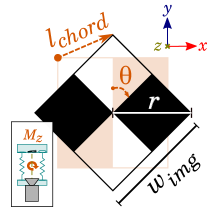
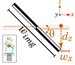
For rotation about the $z$ axis, we can calculate the chord length in pixels traveled when a tag is rotated 45 degrees (about its center), and use the same assumption of four counts per pixel to estimate our rotational sensitivity. Geometrically, we know that

$$l_{chord} =2~{}r\sin\frac{\theta}{2}$$ (14)

In our case, with $w_{img}=$150\text{\,}\mathrm{p}\mathrm{x}$$, we see that

$$\mathit{r} =\sqrt{2}\cdot w_{img}/2$$ (15)

$$l_{chord} =2\sqrt{2}\cdot 150/2\cdot\sin\frac{\pi/4}{2}=$81.18\text{\,}\mathrm{p}\mathrm{x}$$$ (16)

$$s_{\tau z} =\frac{\theta}{l_{chord}}\cdot d_{R}=\frac{81.18}{150}\cdot\frac{1}{4}=$$$$ (17)

For rotation about the $x$ and $y$-axes, the analysis becomes a matter of determining the $z$-axis change in mm, and using that to determine the pixels changed in the $x$-$y$ plane. Consider a 45 degree rotation around the $z$-axis of a tag that starts out flat (facing the camera), as shown in Fig. 6(b). Using $w_{img}=$150\text{\,}\mathrm{p}\mathrm{x}$$ as before, the $z$ sensitivity is as follows:

$$w_{img}/2 =\sqrt{2}\cdot d_{z}$$ (18)

$$d_{z}+w_{x} =w_{img}/2$$ (19)

$$w_{x} =0.5\;w_{img}-\frac{0.5\;w_{img}}{\sqrt{2}}=$21.97\text{\,}\mathrm{p}\mathrm{x}$$$ (20)

$$s_{\tau xy} =\frac{\theta}{w_{x}}d_{R}=\frac{$$}{21.97}\cdot\frac{1}{4}=$$$$ (21)

III-C Notes on z-axis measurements

Intuitively, we expect that the sensor is much less reliable in the $z$ displacement direction. For movement along the $x$ and $y$-axes axes, the camera sees the entire set of black/white intersections moving left or right.

For the same reason, in the single tag setup it would be easy to detect rotations about the $z$-axis, and difficult to detect rotations around the $x$ and $y$-axes. Data collected from this initial (single-tag) design exactly reflected the aforementioned issue. Consequently, the design was enhanced with two tags oriented at 45 degrees to the camera. This proved sufficient for recovering all six force/torque axes.

III-D Force Range Versus Sensitivity

There is a clear trade-off between sensitivity (minimum detectable change in force) and the maximum force range. As an example, for a desired force range $F_{range}=\pm$1\text{\,}\mathrm{N}$=$2\text{\,}\mathrm{N}$$ (close to the observed force range for our prototype), and a maximum displacement of $y_{range}=h_{frame}-h_{img}$, the $y$ sensitivity $s_{y}$ in Newtons is as follows.

$$s_{y} =\frac{F_{range}}{C\cdot y_{range}}=\frac{2}{4\cdot(480-240)}=$0.0021\text{\,}\mathrm{N}$$$ (22)

Our $s_{y}$ is thus 2.1 mN (given our assumption of $d_{R}=0.25$). Similarly, for the $x$-axis we find a sensitivity $s_{x}$ = $1.0\text{\,}\mathrm{m}\mathrm{N}$ at this force range. Now consider instead the grasping use case, with a desired force range of $\pm$ 40 N, and desired sensitivity of at least 0.1 N. If we scale the calculations in Eq. 22 by 40 to get a $\pm$ 40 N force range while keeping the other parameters the same, the sensor has 0.04 N and 0.08 N sensitivities in the $x$ and $y$ directions respectively.

IV Sensor Prototype Evaluation

IV-A Linearity

In order to evaluate the linearity (and therefore usefulness) of the sensor, we used a commercial force-torque sensor (Model HEX-58-RE-400N, OptoForce, Budapest, Hungary) to provide ground truth measurements. Although the OptoForce measures force and torque at a different origin than where the load is applied, the analysis of the linearity of the sensor holds. Data was collected with a Python script which used the OpenCV library to interface with the camera. The setup is shown in Fig. 7.

(a) Experimental setup.

(b) Calibration method.

Figure 7: Left, the data collection setup is shown (with the LED off – note that out-of-frame, there is an Arduino supplying $3.3\text{\,}\mathrm{V}$ to the LED. Later designs used a 3.3 V coin cell battery to make the sensor standalone). Right, a method to calibrate the sensor without using the commercial sensor is demonstrated. The sensor is mounted upside down and weights are hung by string from the sensor to apply force uniaxially to the +$z$ axis.

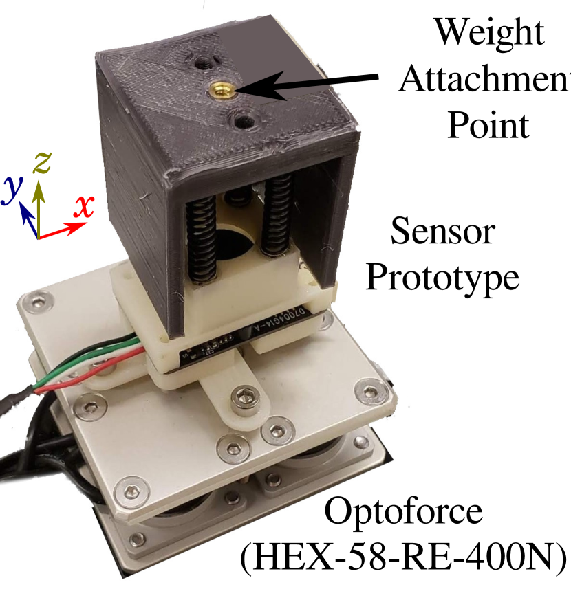
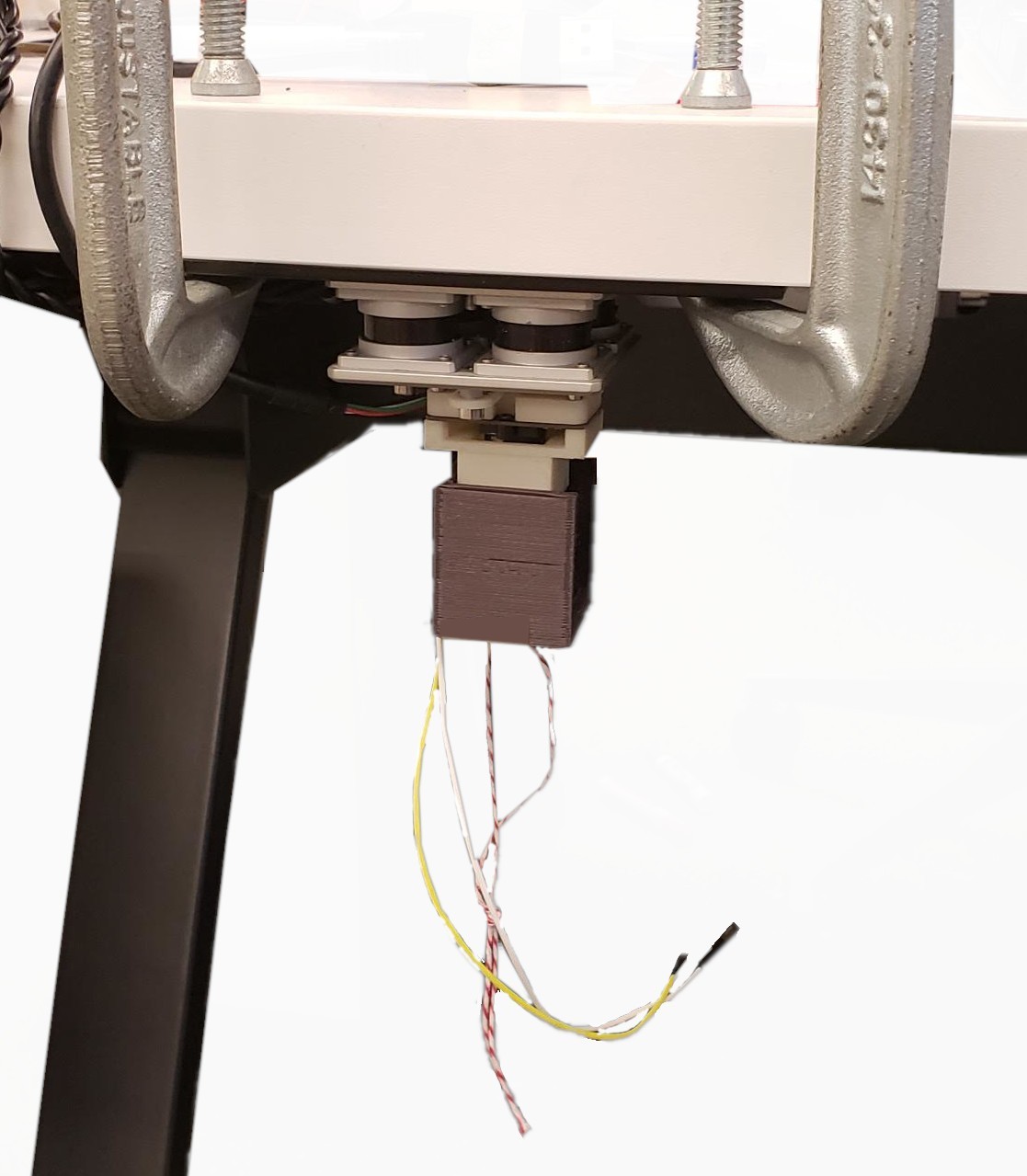
Autocorrelation was used to determine the lag between our sensor and the OptoForce. The sensor lag between the prototype sensor and the OptoForce was roughly 40 milliseconds. Next, linear interpolation was used to match our sensor data with the OptoForce data, which were output at roughly 25 Hz and 125 Hz respectively. The sensor data was smoothed with an exponential filter with weight of 0.2 to improve the autocorrelation results.

For calibration, we take a dataset of displacements $D$ and apply linear regression (with an affine term) against all six axes. $\theta$, $\phi$, and $\gamma$ refer to rotation around the $x$, $y$, and $z$ axes respectively. $K$ then forms a 6-by-6 matrix as shown below.

$$\begin{bmatrix}F_{x}\\ F_{y}\\ F_{z}\\ M_{x}\\ M_{y}\\ M_{z}\end{bmatrix}=\left[\begin{array}[]{cccccc}\cr\\ &&K_{6\times 6}&&&\\ \cr\\ \end{array}\right]\begin{bmatrix}D_{x}\\ D_{y}\\ D_{z}\\ D_{\theta}\\ D_{\phi}\\ D_{\gamma}\end{bmatrix}+\begin{bmatrix}\cr\\ B\\ \cr\\ \end{bmatrix}$$ (28)

IV-B Bandwidth

Sensor bandwidth is directly limited by the camera framerate. This must be physically measured since the Python script will output at unrealistically high framerate – the OpenCV library reads from a buffer of stale images and will return a result even if the camera has not physically delivered a new frame. The webcam is pointed at a display with high refresh rate. A script turns the screen black, and as soon as the camera detects the black color, the screen changes to white, and so forth, and the frames displayed is compared to system time to obtain the framerate of the webcam.

Note that this calculates our maximum sensor bandwidth; our actual sensor bandwidth is determined by the tag detection rate. If dynamic instead of quasi-static loading is assumed, then motion blur can lead to tag detection failure.

V Results

V-A Linearity

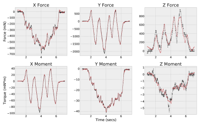
In multiaxial loading, the sensor was manually moved around in all directions. As shown in Fig. 8, the fits had a $R^{2}$ of 0.991, 0.996, 0.875, 0.997, 0.997, and 0.902 for the $F_{x},F_{y},F_{z},M_{x},M_{y}$, and $M_{z}$ axes respectively. The $F_{z}$ axis fit is notably worse than the $F_{x}$ and $F_{y}$ fits, which was expected as explained in Section III-C.

Figure 8: The black line represents a perfectly linear response between our sensor and the commercial sensor. The red dots show the actual sensor measurements using the ArUco tags.

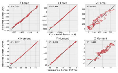
For qualitative comparison, Fig. 8 shows an example of a reconstructed dataset, where the linear fits are plotted against the original signal for qualitative comparison. This diagram shows the relatively large deviations in $F_{z}$ from the original signal, indicating noisiness in the tag measurements.

Figure 9: For qualitative inspection, a compound-loading dataset is shown here. The commercial sensor measurements are in black, and the interpolated and linearly fitted prototype sensor’s measurements are shown in red.

V-B Bandwidth

Our maximum sensor bandwidth is experimentally determined to be 25 Hz. Additionally, the camera we used was one of three cameras bought by selecting for low cost, quick availability, and lack of external camera case. We also measured the other two cameras which, despite advertising similar framerates, exhibited noticeable differences in framerate. Operating at 640x480, we measured 25 fps, 33 fps, and 15 fps for the three cameras, as listed in Table I.

TABLE I: Camera Specifications

Camera Module Name	Nominal Max Res.	Price	Year	FPS @ 640p
D7004G14-A (ours)	1280*720p@30fps	$20	N/A	25
OV 2710	1920*1080@30fps	$20	2017	33
ELP Super Mini	1280*720p@30fps	$30	2015	15

VI Discussion

Our prototype sensor showed mostly linear responses under dynamic loading. While the linearity is not precise, these results still validate the underlying hypothesis that with fiducials it is possible to collect data on all three axes of force and three axes of torque. Further design iterations could improve on these results, although this approach is unlikely to achieve the  0.1 sensors.

VI-A Design Goals

The sensor can now be evaluated against the goals specified previously in Section II-B. The sensor design is indeed responsive in all six axes (after our pivot from one tag to two tags, as well as using a much brighter LED). Additionally, for grasping applications, the calculations in Eq. 22 shows that if a much stiffer spring were chosen so that 40 N of load could be applied without exceeding the $y_{range}$, the sensor would still have better than 0.1 N of sensitivity.

The qualitative design goals were also met. The sensor is small, measuring only 3.6 cm by 3.1 cm by 5.1 cm in size. The sensor is inexpensive, with the majority of the cost being a $20 webcam. The sensor is robust and has survived multiple plane trips and the occasional throw or drop. The sensor is also easy to modify. The light shield can easily be unbolted to change the fiducials, or re-printed in an hour to accommodate different designs (e.g. a single-tag vs. dual-tag design). Fabrication is easy and non-toxic, requiring no degassing machine (as with elastomer-based sensors) nor electrical discharging machines (as with custom strain-gauge based designs). The sensor by design does not suffer from thermal considerations (as in [8]) or electrical noise (as with designs based on strain gauges).

VI-B Error Sources

An important consideration is the coordinate origin around which measurements are made. As load must be applied to the spring platform on which the tags are glued, the origin around which measurements are collected may be different than desired, although a linear offset matrix should suffice to correct for this. Our six-axis measurement reflects a combination of a camera pose estimation and mechanical coupling, each of which can introduce errors. In the following section on sensor improvement, we focus on camera sensor issues.

VI-C Sensor Improvements

VI-C1 Fiducial Changes

Unlike the standard use cases for ArUco markers, we do not care about distinguishing multiple objects and care more about the quality of the pose estimate for a tag guaranteed to be in-frame. A custom fiducial (perhaps solely a checkerboard) could improve the force-torque measurements.

VI-C2 Noise in z-axis

The sensor is noisy in force and torque measurements along the $z$-axis. To address this, one possibility is to use a mirror and two tags which are laid flat on the $xy$ plane and the $yz$ plane respectively. The “sideways” tag (on the $yz$ plane) has good sensitivity to $z$-axis displacements, and the flat $xy$ plane tag is addresses rotations around the $z$-axis. A 45-degree mirror then allows the camera to also observe the ”sideways” tag on the $yz$ plane. On the downside, the small mirror could make assembly difficult.

VI-C3 Sensor Size

Closer placement of the tag, to minimize the size of the sensor, may also be desired – this would necessitate a custom lens for the camera to allow for closer focus (e.g. a macro lens). Miniaturization could also be accomplished with a smaller camera, as in [3].

VI-C4 Replacing Springs

The use of springs means that the sensor may behave poorly in high frequency domains. Replacing the springs with another mechanism, such as a Stewart platform, could allow custom tuning of the response. Another possibility would be to fill the gap between the camera and the tag with optically clear material that would be resistant to high frequency inputs. [16] used a similar idea with a magnet and hall effect sensor, for a three-axis force sensor. However, such a design would complicate fabrication and potentially make camera calibration difficult due to image warping.

TABLE II: List of components and approximate costs.

Part	Details	Cost
Camera	Mini Camera module, AmazonSIN: B07CHVYTGD	$20
LED and 2 wires	Golden DRAGON Plus White, 6000K, 124 lumens	$2
4 springs	Assorted small springs set	$5
3D printed pieces	PLA filament	$5
Heat-set Threaded Inserts	Package of 50 from McMaster-Carr (use 2)	$1
Misc. Bolts	Hex socket head	$1
Epoxy	5 minute	$5

VII Conclusion

We present a novel type of six-axis force-torque sensor using fiducial tags and a webcam. The design is fast to fabricate and simple to use, and is also strong enough to survive drops and crashes common in contact-rich tasks such as robotic grasping. With only 3D-printed custom components, the design needs minimal technical expertise to adapt to applications ranging from manipulation to human-computer interaction research. The open-source design also allows for direct integration in designs for tasks such as grasping where sensor size is important. This fiducial-based sensor is less accurate than commercial force-torque sensors, but is also orders-of-magnitude less expensive – commercial sensors can cost thousands of dollars, while the parts cost of our sensor is under $50 (see Table II). These combined advantages of our prototype sensor validates the general design principle of using 3D pose estimates from printed fiducials to create a six-axis force-torque sensor. Future work on improving the $F_{z}$ and $M_{z}$ axes could allow for an inexpensive, user-friendly, and robust alternative to current commercial sensors, opening up a new range of use cases for six-axis force-torque sensors.

References

- [1] W. Yuan, R. Li, M. A. Srinivasan, and E. H. Adelson, “Measurement of shear and slip with a gelsight tactile sensor,” 2015 IEEE International Conference on Robotics and Automation (ICRA), pp. 304–311, 2015.
- [2] K. Sato, K. Kamiyama, N. Kawakami, and S. Tachi, “Finger-shaped gelforce: Sensor for measuring surface traction fields for robotic hand,” IEEE Transactions on Haptics, vol. 3, pp. 37–47, 2010.
- [3] B. Ward-Cherrier, N. Pestell, L. Cramphorn, B. Winstone, M. E. Giannaccini, J. Rossiter, and N. F. Lepora, “The tactip family: Soft optical tactile sensors with 3d-printed biomimetic morphologies,” in Soft robotics, 2018.
- [4] A. Yamaguchi and C. G. Atkeson, “Combining finger vision and optical tactile sensing: Reducing and handling errors while cutting vegetables,” 2016 IEEE-RAS 16th International Conference on Humanoid Robots (Humanoids), pp. 1045–1051, 2016.
- [5] F. Beyeler, S. Muntwyler, and B. J. Nelson, “A six-axis mems force–torque sensor with micro-newton and nano-newtonmeter resolution,” Journal of Microelectromechanical Systems, vol. 18, pp. 433–441, 2009.
- [6] P. Estevez, J. Bank, M. Porta, J. Wei, P. Sarro, M. Tichem, and U. Staufer, “6 dof force and torque sensor for micro-manipulation applications,” Sensors and Actuators A: Physical, vol. 186, pp. 86–93, 2012.
- [7] D. J. Cappelleri, G. Piazza, and R. V. Kumar, “Two-dimensional, vision-based n force sensor for microrobotics,” 2009 IEEE International Conference on Robotics and Automation, pp. 1016–1021, 2009.
- [8] J. Guggenheim, L. P. Jentoft, Y. Tenzer, and R. D. Howe, “Robust and inexpensive six-axis force–torque sensors using mems barometers,” IEEE/ASME Transactions on Mechatronics, vol. 22, pp. 838–844, 2017.
- [9] M. S. Sun Yu, Hollerbach John, “System, method and apparatus for detecting a force applied to a finger,” U.S. Patent 20 080 091 121, 2008.
- [10] A. Sartison, D. Mironov, K. Youcef-Toumi, and D. Tsetserukou, “Finger grip force estimation from video using two stream approach,” CoRR, vol. abs/1803.01630, 2018.
- [11] E. Olson, “Apriltag: A robust and flexible visual fiducial system,” 2011 IEEE International Conference on Robotics and Automation, pp. 3400–3407, 2011.
- [12] S. Garrido-Jurado, R. Muñoz-Salinas, F. J. Madrid-Cuevas, and M. J. Marín-Jiménez, “Automatic generation and detection of highly reliable fiducial markers under occlusion,” Pattern Recognition, vol. 47, pp. 2280–2292, 2014.
- [13] G. Bradski, “The OpenCV Library,” Dr. Dobb’s Journal of Software Tools, 2000.
- [14] (2018) Ros driver for the optoforce sensor. [Online]. Available: https://github.com/shadow-robot/optoforce
- [15] J. Mellado. (2018) js-aruco: Javascript library for augmented reality applications. [Online]. Available: https://github.com/jcmellado/js-aruco
- [16] R. Kõiva, T. Schwank, R. Haschke, and H. J. Ritter, “Fingernail with static and dynamic force sensing,” in Fingernail with static and dynamic force sensing, 2016.