Electric charge estimation using a SensL SiPM

Abstract

The silicon photo-multipliers (SiPMs) are commonly used in the construction of radiation detectors such as those used in high energy experiments and its applications, where an excellent time resolution is required for triggering. In most of this cases, the trigger systems electric charge information is discarded due to limitations in data acquisition. In this work we propose a method using a simple radiation detector based on an organic plastic scintillator $2\times 2\times 0.3$ cm³ size, to estimate the electric charge obtained from the acquisition of the fast output signal of a SensL SiPM model C-60035-4P-EVB. Our results suggest a linear relation between the reconstructed electric charge from the fast output of the SiPM used with respect to the one reconstructed with its standard signal output. Using our electric charge reconstruction method, we compared the sensitivity of two plastic scintillators, BC404 and BC422Q, under the presence of Sr90, Cs137, Co60, and Na22 radiation sources.

Keywords Scintillators  $\cdot$ Trigger detectors  $\cdot$ PET PET/CT

1 Introduction

Silicon Photomultipiers (SiPM) have been widely used during the past two decades in different areas like high energy physics [2, 1], and its medical applications. A clear example is the development of Positron Emission Tomography (PET)[3] where the typical photo multiplier tube (PMT) is being replaced by the SiPM technology with the aim to improve its time and spatial resolutions [6, 5, 4, 7]. Since 2013 SensL corporation has developed SiPMs with two signal outputs: Standard and fast [8]. For a $6\times 6$ mm³ of SensL C-series SiPM, the standard signal output is characterized by a raise time of 4 ns and a pulse width of 100 ns, while the raise time of the fast signal output is 1 ns with a pulse width of 3.2 ns [9].

Several works have reported the use of SiPMs [1, 3, 10, 11, 12], where the standard output is commonly used to reconstruct the deposited electric charge using the acquired photo current from the anode which is related with the deposited energy in the sensitive material of a radiation detector [5, 11, 13, 14]. In recent years, the fast signal output has been used to improve the pulse shape discrimination of gammas and fast neutrons [2, 15]. It has been also shown that exists an equivalent coincidence resolving time (CRT) between the fast and standard output signals of the SensL SiPM [16]. An application for this fast pulse, is on a detector development with high time resolution as described in [17]. In this work we use a simple radiation detector based in organic plastic scintillator to study the relation of the reconstructed electric charged using both SensL SiPM output signals.
This work is organized as follows. In Section 2 the methodology of this work is described. In Section 3 we present the analysis and discussions of the results. Finally, in Section 4 we present our conclusions.

2 Materials and method

2.1 Instrumentation

A MicroFC-60035 SiPM from SensL with a cell size of 35 $\mu$m, peak wavelength of 420 nm and package size of $6\times 6$ mm² was used. In order to acquire the two signals from this SiPM, we developed a homemade printed circuit board (PCB) of $3\times 4$ cm, specifically designed for the described SiPM model. The schematic diagram is shown in Figure 1, where $V_{s}$ and $V_{f}$ refers to the standard and the fast output signal, respectively. As described in [9], an overvoltage of $V_{br}$+5 V was used to maximize the photon detection efficiency (PDE) of the SiPM.

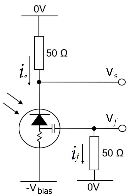
Figure 1: Basic front-end electronics for polarization and acquisition of standard and fast signals.

We choose BC404 [18] and BC422Q [19] plastic scintillator as radiation sensitive materials, with a volume of $20\times 20\times 3$ mm³. Some scintillation characteristics are shown in Table 1 [20]. The BC422Q material was selected with a weight percentage of benzophenone of $0.5\%$.

Table 1: Scintillator material properties. [20]

	BC404	BC422Q
Rise Time (ps)	700	110
Decay Time (ns)	1.8	0.7
Pulse Width, FWHM (ps)	2,200	360

The experimental setup is shown in Figure 2, where the SiPM was attached to the center of each plastic scintillator and a radioactive source was located in the opposite face. Four radioactive sources were used: ⁹⁰Sr, ²²Na, ¹³⁷Cs and ⁶⁰Co so, the description for these radioactive sources is shown in Table 2.

Figure 2: Experimental setup scheme, showing the fast and standard outputs.

Table 2: Radiation sources properties.

Source	Radiation	Gamma 1	Gamma 2	Beta
	[$\mu$Ci]	[keV]	[keV]	[keV]
60Co	1.00	1173	1332	-
137Cs	0.25	662	-	-
22Na	1.00	511	1275	-
90Sr	0.10	-	-	546

A Tektronix DPO7054 digital oscilloscope was used for signal acquisition, with a 50 $\Omega$ of coupling impedance and a sampling rate of 10 GS/s. For each radioactive source, $10^{4}$ events were recorded. Each event consists of $2\times 10^{4}$ samples to reconstruct the pulse. The reconstruction and the data analysis was made offline with CERN ROOT software [21].

2.2 Methods

2.2.1 Linear regression

We reconstruct the electric charge from the fast ($Q_{F}$) and standard ($Q_{S}$) output signals, using the integrals given in equations(1) and (1).

$$Q_{S} =\int_{t_{i}}^{t_{f}}i_{s}(t)dt=\frac{1}{50}\int_{t_{i}}^{t_{f}}V_{s}(t)dt$$ (1)

$$Q_{F} =\int_{t_{i}^{\prime}}^{t_{f}^{\prime}}i_{f}(t)dt=\frac{1}{50}\int_{t_{i}^{\prime}}^{t_{f}^{\prime}}V_{f}(t)dt$$ (2)

If a linear relation between fast and standard signal outputs is assumed, and supposing $g_{x}$ and $g_{y}$ random variables with Gaussian Probability Distribution Functions (PDF), we can introduce the Pearson’s correlation coefficient given by [23].

$$R_{xy}=\frac{Cov(g_{x},g_{y})}{\sigma_{x}\sigma_{y}}$$ (3)

where $Cov(g_{x},g_{y})$ is defined as the covariance between random variables $g_{x}$ and $g_{y}$, while $\sigma_{x}$ and $\sigma_{y}$ correspond to the standard deviation of $x$ and $y$ variables, respectively. After the described correlation test, a regression line can be adjusted to obtain a linear model based on statistical moments for each stochastic process, as described by the following equation

$$y-\bar{y}=\frac{Cov(g_{x},g_{y})}{\sigma_{x}^{2}}(x-\bar{x})$$ (4)

It can be rewritten in terms of the correlation coefficient as

$$y=\frac{\sigma_{y}}{\sigma_{x}}R_{xy}(x-\bar{x})+\bar{y},$$ (5)

which is a standard equation of a straight line

$$y=ax+b$$ (6)

with

$$a=\frac{\sigma_{y}}{\sigma_{x}}R_{xy}$$ (7)

$$b=\bar{y}-a\bar{x}$$ (8)

In this case, $x$ was defined as the charge $Q_{f}$ measured from the standard signal and $y$ as the charge $Q_{s}$ from fast output signal. Therefore, equations 6 and 7 can be rearranged in terms of charge,

$$Q_{s}=aQ_{f}+b,$$ (9)

$$a=\frac{\sigma_{s}}{\sigma_{f}}R_{fs},$$ (10)

$$b=\bar{Q_{s}}-a\bar{Q_{f}},$$ (11)

where $\sigma_{f}$ and $\sigma_{s}$ refer to standard deviation of fast and standard signal charges, respectively. While $R_{sf}$ is the correlation coefficient between $Q_{s}$ and $Q_{f}$.

As it was mentioned, the linear regression methodology can be applied if the random variables have a Gaussian (PDF) [24], giving the possibility to use the Pearson correlation coefficient. As the PDF acquired from the SensL SiPM are not Gaussian, a non-parametric approach can be used in order to estimate the statistical parameter. This approach makes use of the Spearman correlation index defined by equation 12 [24]

$$R_{rFast,rStd}=\frac{Cov(rFast,rStd)}{\sigma_{rFast}\sigma_{rStd}}$$ (12)

where $rFast$ and $rStd$ correspond to the ranked fast and standard signals, $\sigma_{rFast}$ and $\sigma_{rStd}$ are the standard deviation of ranked fast and standard signals, viewed as random variables [23]. As can be observed in 12, the correlation coefficient definition is the same as Pearson correlation, except that the random variables are ranked [23].

As described in [25], this approach does not depend on the used PDFs so, the mean and variance are calculated from a Gaussian distribution, as commonly used. A second approach to apply the linear regression by fitting a Gaussian PDF to the maximum peaks, observed in the charge deposition histograms from fast and standard signals, as it is shown in Fig 3; thus, mean and variance are calculated. Moreover, both approaches will be used to demonstrate that standard and fast SiPM signals are highly correlated.

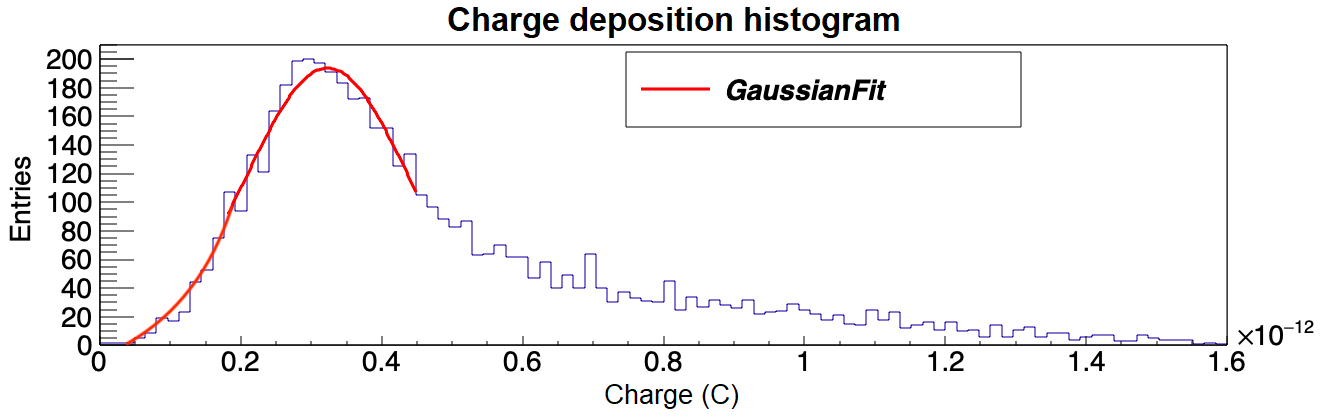
Figure 3: SiPM charge deposition histogram and Gaussian fit for estimation

In CERN root software, the integral was performed on windows of $2\times 10^{3}$ samples for fast signal and $1.6\times 10^{4}$ samples for standard signal, because of tail effect.

2.2.2 Two-samples Kolmogorov-Smirnov test

It is important to make a quantitative comparison among standard and estimated charge deposition. This can be done using the non parametric Two-Sample Kolmogorov-Smirnov (TSKS) test [26] which is useful to evaluate whether two underlying one-dimensional probability distributions differ from each other. The Cumulative Density Function (CDF) for each signal is calculated. In the other hand, the test hypothesis can be represented as follows: for a given CDF $F_{s}$, for charge deposition of the standard SiPM output, and a given empirical CDF $F_{est}$, for the estimated charge deposition, the test statistics divergence $D_{n,m}$ can be written as: [26]

$$D_{n,m}=Max_{x}|F_{s,n}(x)-F_{est,m}(x)|$$ (13)

where $n$ and $m$ correspond to the CDF size of the standard and estimated deposited charge. $Max_{x}$ represents the maximum of the distances set. Moreover, equation 13 compares the empirical CDF’s from the two charge deposition random variables under test, in order to find out whether both random variables come from same distribution or not. The Kolmogorov-Smirnov (KS) test statistic $\sqrt{n}D_{n,m}$ will help to reject the null hypothesis at level of significance $\alpha$ if $\sqrt{n}D_{n,m}>K_{\alpha}$ for $m,n\to\infty$, where $P(K<K_{\alpha})=1-\alpha$. Thus, the associated $p-value$ is calculated from tables or algorithms, in our case MATLAB was used to apply the KS-test to both CDF’s. The resulting $p-value$ is compared with the level of significance $\alpha$ so, the null hypothesis is related to equation 14

$$H_{0}:F_{s}=F_{est}:Failure~{}to~{}reject~{}the~{}null~{}hypothesis~{}at~{}the~{}\alpha-level$$ (14)

$$H_{1}:F_{s}\not=F_{est}:Rejection~{}of~{}the~{}null~{}hypothesis~{}at~{}the~{}\alpha-level$$ (15)

3 Analysis and results

To determine the relation between standard and fast charges, the correlation coefficient was calculated for each radiation source (Co60, Cs137, Na22 and Sr90) and each plastic scintillator (BC404 and BC422Q). As the probability distribution functions for deposited charge from a SiPM are non Gaussian, Pearson correlation index cannot be estimated; therefore, the described approaches from section 2 were used. From the first approach, Spearman correlation coefficient was estimated after data ranking for standard and fast charge estimations [22]. Then, a Gaussian fit was applied to each distribution for standard and fast charge estimations, resulting on mean and variance calculation and, thus, a Pearson correlation coefficient as reported in Table 3.

Table 3: Correlation $R_{sf}$ between $Q_{s}$ and $Q_{f}$

-	BC404		BC422Q
Source	Pearson	Spearman	Pearson	Spearman
Co60	0.9686	0.9489	0.9783	0.9611
Cs137	0.9484	0.9157	0.9367	0.9111
Na22	0.9549	0.9414	0.9767	0.9320
Sr90	0.9658	0.9522	0.9856	0.9660

Correlation coefficient was estimated, resulting on indexes close to one as observed on Table 3, which confirms the linear relation hypothesis for fast and standard reconstructed electric charge. Therefore, the described linear regression in Equation 4 can be applied to reconstruct the charge distribution for the standard output from the fast signal. This relation is depicted in Figure 4, where, the estimated charge correlation for each radioactive source was graphed. The BC422Q plastic scintillator produces a lower number of photons with respect to BC404. The BC404 has a 68% of athracene and the BC422Q has a 19% [18, 19]. Thus, the BC404 emits more photons than BC422Q. A detailed discussion about the properties of plastic scintillators can be found in [27].

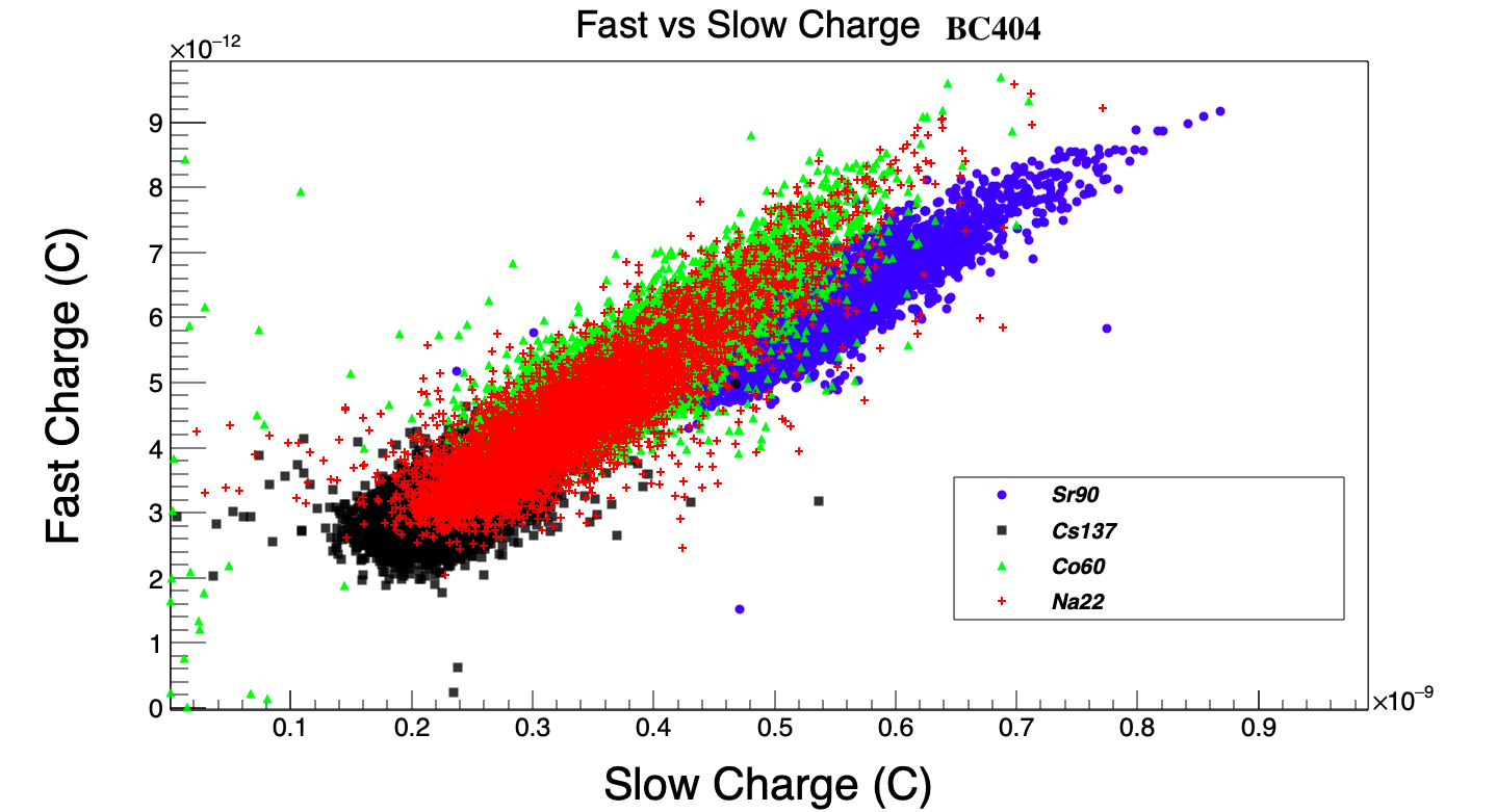
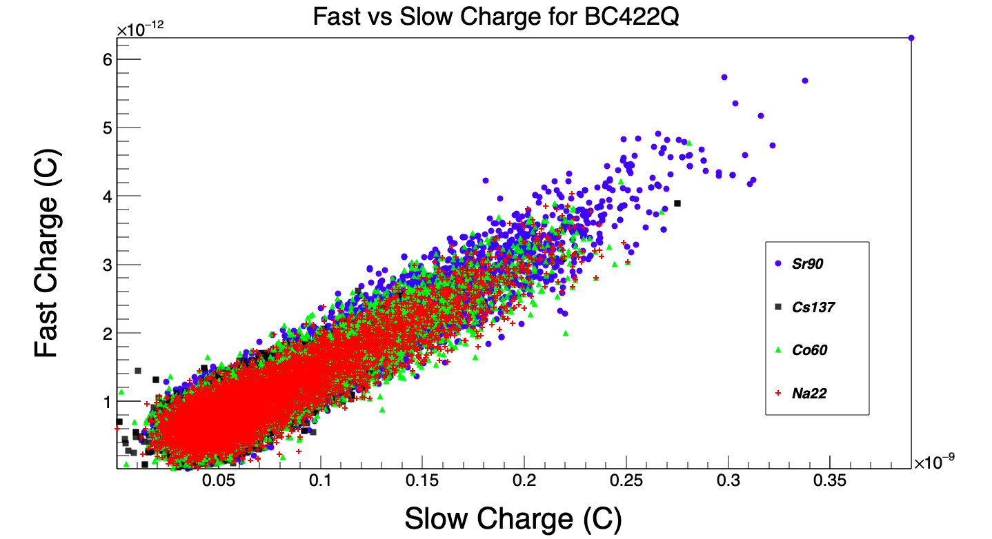
Figure 4: Scatter plot for integrated fast and standard output signals using (left) BC404 and (right) BC422Q scintillators.

Two orders of magnitude from fast and standard charge can be observed, which is related to the difference of charge deposition among the two variables of interest. Also, it is possible to qualitatively distinguish between the four sources for the case of BC404 scintillator, giving an opportunity for future development of classification algorithm implementation. In particular, ⁹⁰Sr and ¹³⁷Cs can be clearly separated from ²²Na and ⁶⁰Co. For the case of BC422Q scintillator, this source separation seems to be harder to accomplish.

The mean and standard deviation are the required statistical momenta for the linear regression model. As an example, in Figure 5 the charge distribution for the ²²Na radioactive source and both scintillator materials, BC404 and BC422Q, is shown . Doing a Gaussian fit on the the peaks, it is possible to get the required momentum. A particular case is observed for this source, two peaks can be appreciated in fast and standard charge for BC404 scintillator. One of these peaks can be associated to the original gamma from the source and the other can be associated to a gamma from the pair annihilation from positron emission. For BC422Q scintillator, a single peak is observed for this material. The rest of the sources for both materials have the same shape of one peak.

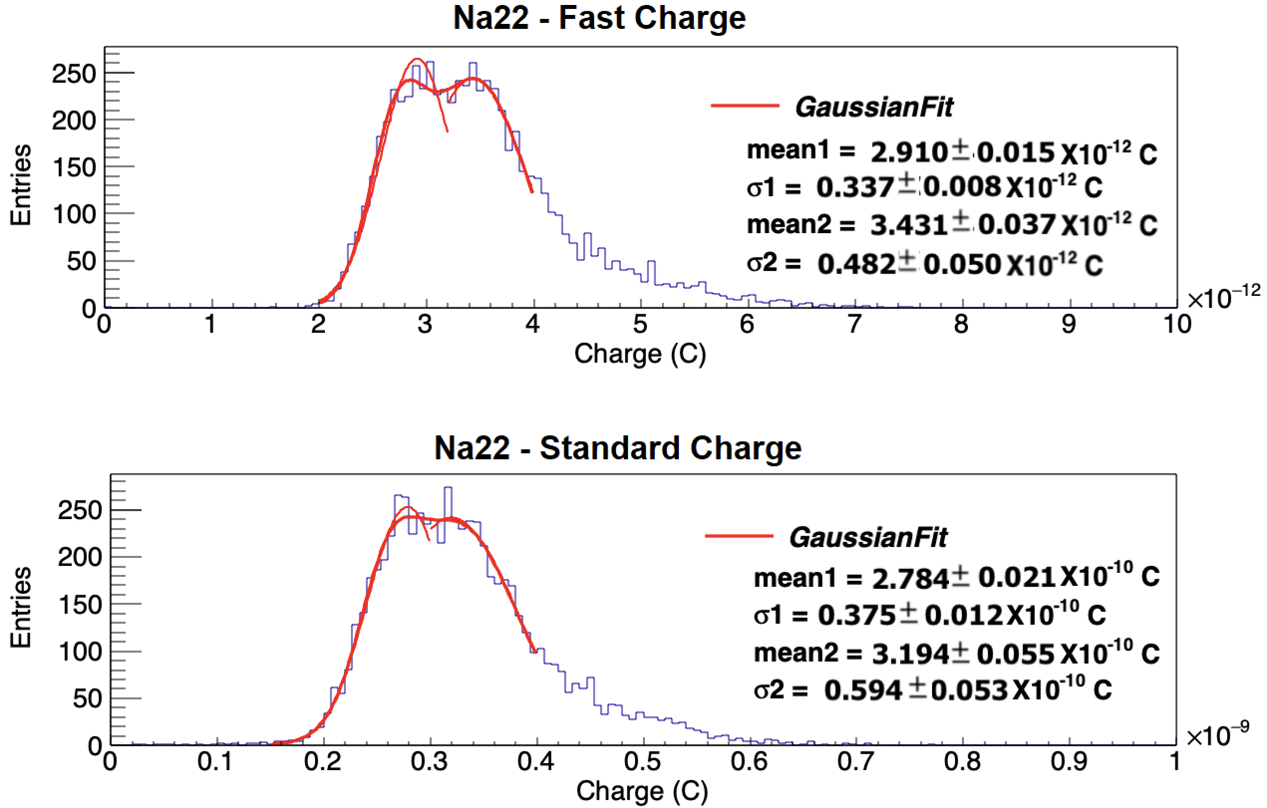
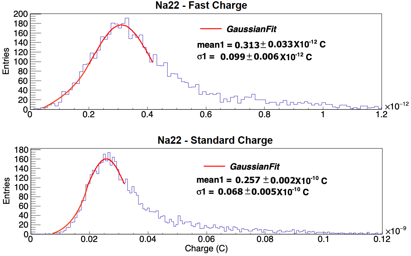
Figure 5: ²²Na charge deposition comparison and fit for fast and standard outputs for BC404 (left) and BC422Q (right) scintillators.

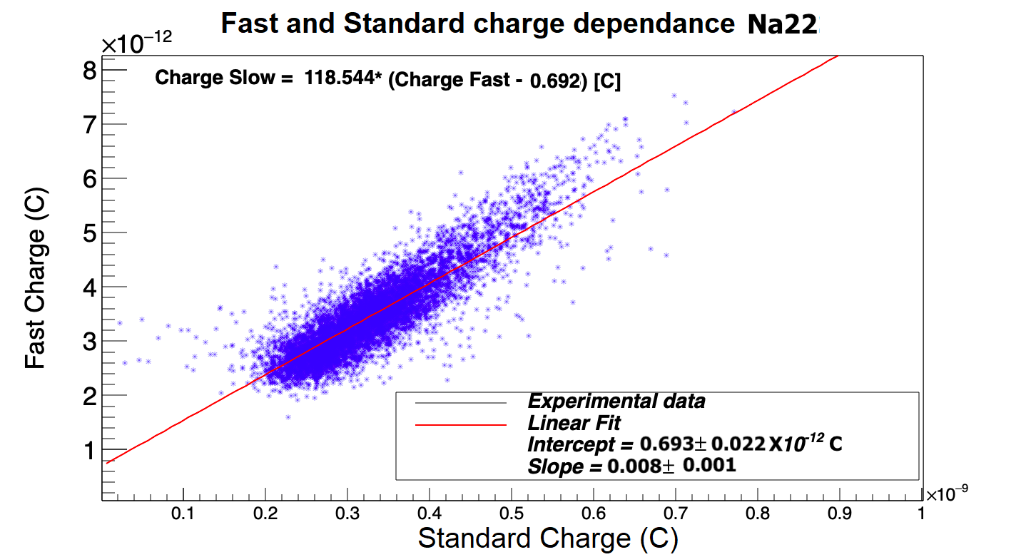
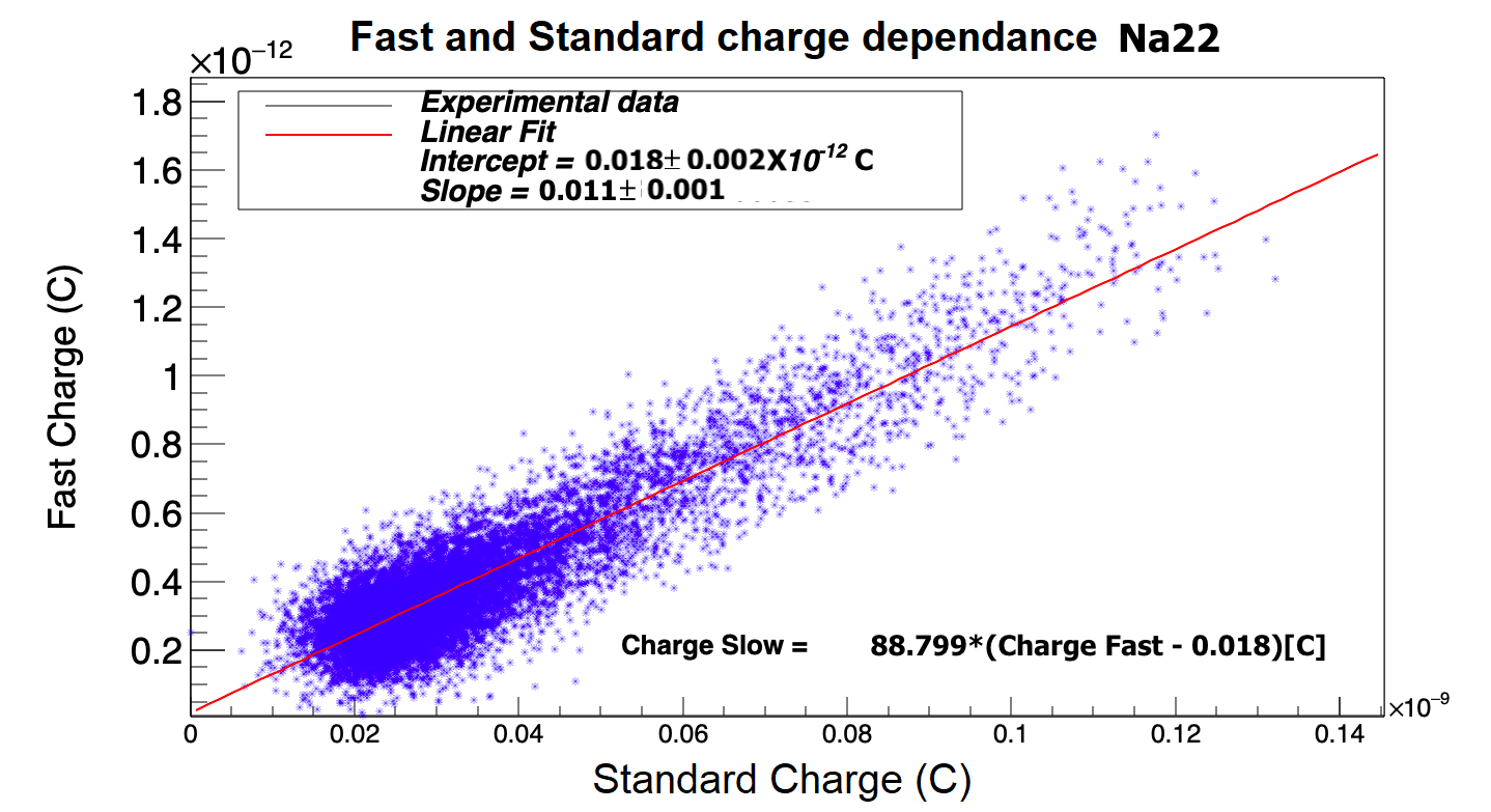
Figure 6: Relation between the fast and standard charge for BC404 and BC422Q.

Once the linear relation between fast and standard charge has been established, all parameters required in the model were calculated. For each random variable, the correlation index $R_{sf}$, the mean $\bar{Q_{s}}$ and $\bar{Q_{f}}$ and standard deviations $\sigma_{s}$ and $\sigma_{f}$ were estimated. To exemplify this relation, in Figure 6 is shown the linear dependence for ²²Na source from BC404 and BC422Q scintillator materials. For a complete reference about the the resulting parameters, the measurements are listed in Tables 4 and 5 for BC404 and BC422Q scintillators, respectively. Based on results from Tables 4 and 5, the linear regression parameters for each source and material are shown in Tables 6 and 7 for BC404 and BC422Q scintillator, respectively.

Table 4: BC404 scintillator material linear regression estimated parameters

Source	$\bar{Q_{f}}$	$\sigma_{f}$	$\bar{Q_{s}}$	$\sigma_{s}$
-	[$10^{-12}C$]	[$10^{-12}C$]	[$10^{-10}C$]	[$10^{-10}C$]
22Na${}_{peak_{1}}$	2.910	0.338	2.784	0.374
22Na${}_{peak_{2}}$	3.431	0.482	3.194	0.594
90Sr	5.492	0.314	5.127	0.373
137Cs	2.450	0.345	2.297	0.355
60Co	3.648	0.259	3.464	0.433

Table 5: BC422Q scintillator material linear regression estimated parameters

Source	$\bar{Q_{f}}$	$\sigma_{f}$	$\bar{Q_{s}}$	$\sigma_{s}$
-	[$10^{-12}C$]	[$10^{-12}C$]	[$10^{-10}C$]	[$10^{-10}C$]
22Na	0.311	0.099	0.258	0.068
90Sr	0.323	0.116	0.262	0.074
137Cs	0.333	0.131	0.269	0.082
60Co	0.323	0.120	0.263	0.080

Table 6: Linear regression(BC404).

Source	a	a (error)	b	b (error)
-	[$10^{-3}$]	[$10^{-5}$]	[$10^{-12}$C]	[$10^{-12}$C]
60Co	7.75	6.3	1.14	0.03
137Cs	6.18	9.9	1.06	0.22
22Na	8.43	9.3	0.69	0.02
90Sr	9.06	5.5	0.95	0.03

Table 7: Linear regression(BC422Q)

Source	a	a (error)	b	b (error)
-	[$10^{-2}$]	[$10^{-5}$]	[$10^{-12}$C]	[$10^{-15}$C]
60Co	1.16	5.3	0.014	2.30
137Cs	1.01	9.4	0.052	3.10
22Na	1.13	5.5	0.017	2.22
90Sr	1.17	4.3	0.004	2.11

Using the respective linear regression from Tables 6 and 7, it is possible to reconstruct the original charge distribution from the fast pulse. In Figure 7 the reconstructed charge distribution for ²²Na and both materials is shown (note that the two peaks for BC404 are reconstructed). We make a statistical analysis to compare the original and reconstructed charge. In Tables 8 and 9 the fit parameters for all sources and both materials are shown.
As an additional test, we computed the ratio between the integral value of both distributions, reconstructed and original. These values are shown in Table 10.

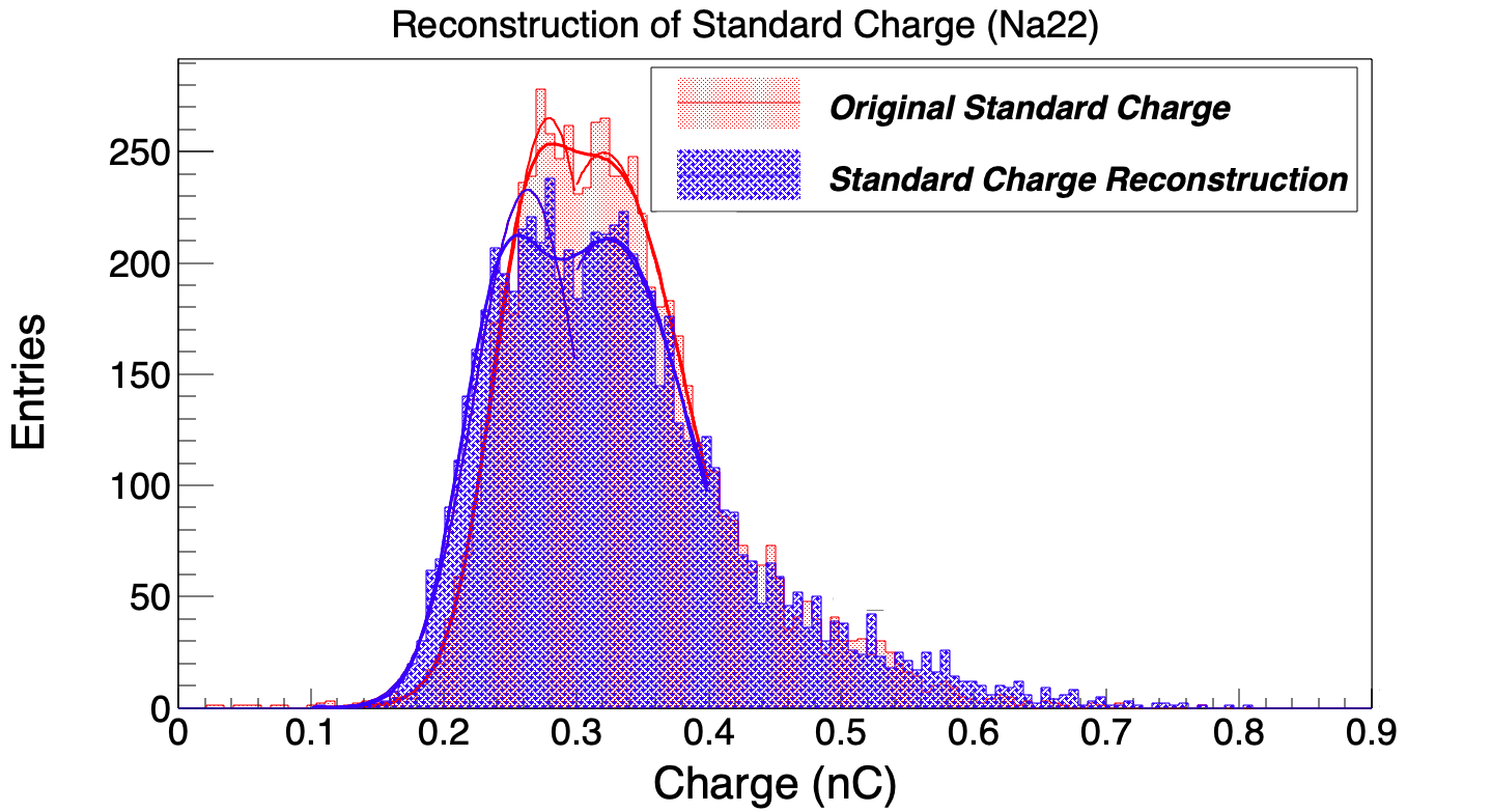
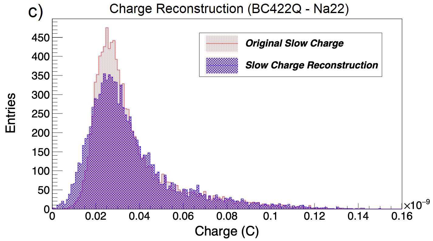
Figure 7: Original and reconstructed charge distributions for Bc404 (left) and BC422Q (right) for ²²Na

Table 8: Gaussian Fit parameters for Bc404. ^othe original charge. ^rthe reconstruction charge. ${}^{1,~{}2}$the fit parameters for the first and second Gaussian in ²²Na distribution, respectively.

Source	Mean (nC)	Error Mean (nC)	$\sigma$ (nC)	Error $\sigma$ (nC)
22Na	0.2795o,1	0.0023o,1	0.0380o,1	0.0012o,1
	0.3201o,2	0.0044o,2	0.0591o,2	0.0046o,2
	0.2633r,1	0.0016r,1	0.0400r,1	0.0009r,1
	0.3231r,2	0.0053r,2	0.0622r,2	0.0063r,2
90Sr	0.1276o	0.0002o	0.0092o	0.0001o
	0.1257r	0.0002r	0.0088r	0.0001r
137Cs	0.2320o	0.0004o	0.0324o	0.0003o
	0.2257r	0.0009r	0.0380r	0.0007r
60Co	0.3497o	0.0008o	0.0389o	0.0006o
	0.3271r	0.0009r	0.0393r	0.0006r

Table 9: Gaussian Fit parameters for Bc422Q. ^othe original charge. ^rthe reconstruction charge.

Source	Mean (nC)	Error Mean  (nC)	$\sigma$ (nC)	Error $\sigma$  (nC)
22Na	0.0269o	0.0001o	0.0066o	0.0001o
	0.0259o	0.0002o	0.0085o	0.0001o
90Sr	0.0273o	0.0001o	0.0087o	0.0001o
	0.0273r	0.0001r	0.0086r	0.0001r
137Cs	0.0281o	0.0001o	0.0069o	0.0001o
	0.0266r	0.0003r	0.0099r	0.0002r
60Co	0.0271o	0.0001o	0.0070o	0.0001o
	0.0262r	0.0002r	0.0086r	0.0001r

Table 10: Ratio between the area of the original and reconstructed charge distribution.

Source	Ratio area distribution for BC404	Ratio area distribution for BC422Q
${}^{60}Co$	1.0002$\pm$2.2$\times 10^{-5}$	1.0037 $\pm$2.2$\times 10^{-5}$
${}^{22}Na$	1.0001$\pm$1.8$\times 10^{-5}$	1.0019$\pm$1.1$\times 10^{-5}$
${}^{137}Cs$	1.0022$\pm$1.8$\times 10^{-5}$	1.0028$\pm$1.8$\times 10^{-5}$
${}^{90}Sr$	1.0001$\pm$0.1$\times 10^{-5}$	1.0001$\pm$0.1$\times 10^{-5}$

The reconstruction of the charge is performed event by event. Thus, it is possible to make the difference between the original and reconstructed charge value. As an example, in Figure 8, the plots of such differences for ²²Na for both plastic scintillators are shown. From the fit of these distributions, it is possible to obtain the reconstructed charge resolution, $\sigma$. The resolution values for all the used radiation sources for both materials are shown in Table 11. The best reconstructed charge resolution is obtained for BC422Q plastic scintillator in all the cases.

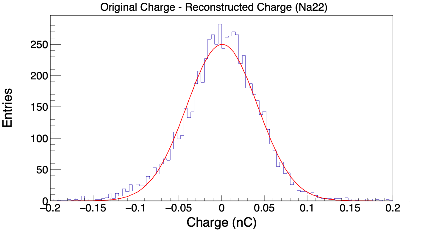
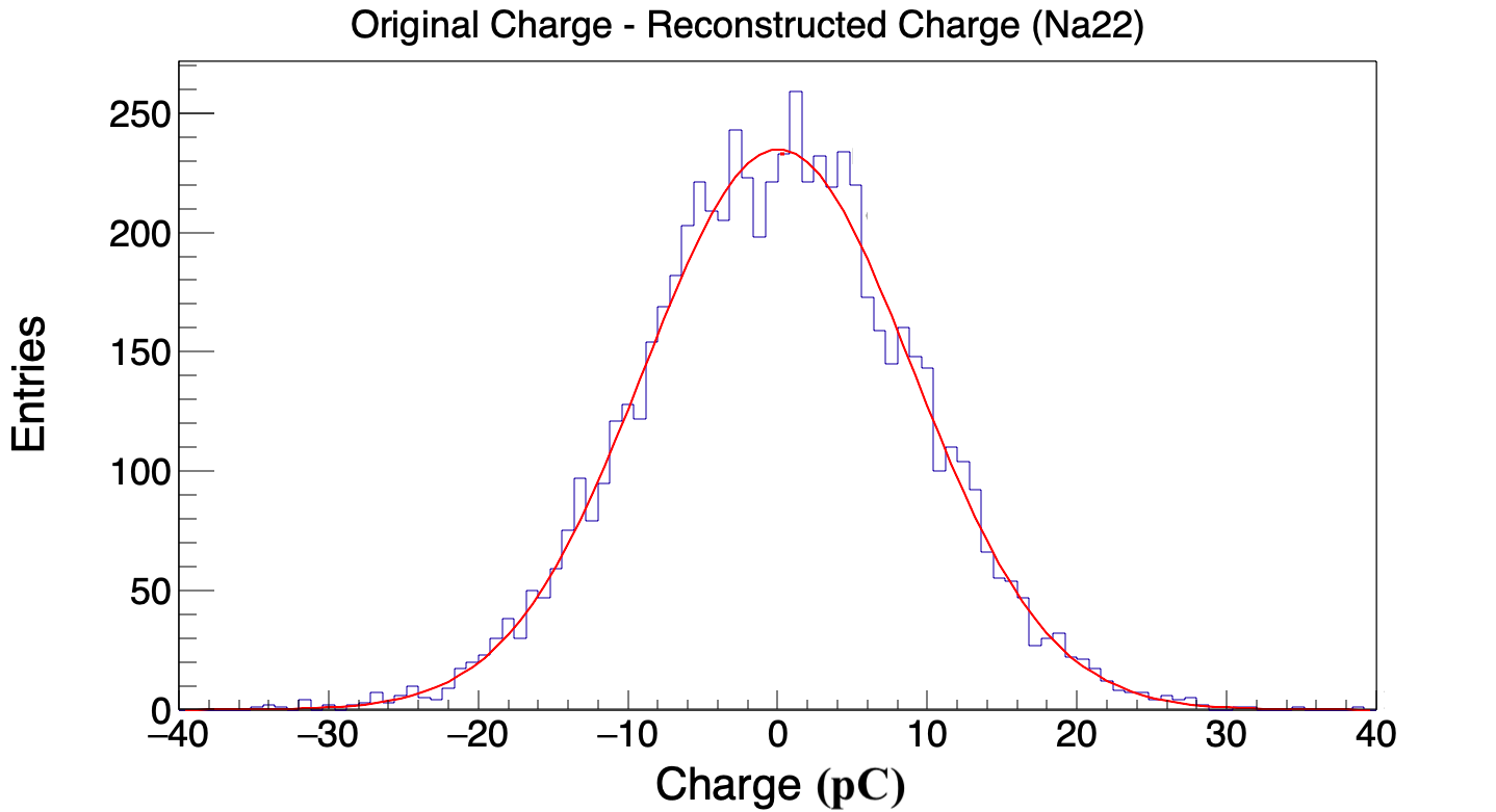
Figure 8: Difference distribution between the original charge and the reconstructed charge for ²²Na and BC404 (left) and BC422Q (right).

Table 11: Resolution reconstructed charge for both materials.

Source	BC404	BC422Q
	$\sigma$ (pC)	$\sigma$ (pC)
${}^{60}Co$	47.2$\pm$0.4	8.9 $\pm$0.1
${}^{22}Na$	41.4$\pm$0.4	8.9$\pm$0.1
${}^{137}Cs$	45.5$\pm$0.4	9.3$\pm$0.1
${}^{90}Sr$	8.0$\pm$0.1	8.9$\pm$0.1

We also applied another test to compare the Probability Density Function (PDF) for the standard and reconstructed charge. The TSKS-test (described in subsection 2.2.2) was applied to both distributions. The CDF’s for each radiating source and scintillator material are shown in Figures 9 and 10. The results of this test are listed in the Table 12. We noted that the corresponding CDF’s are equivalent for the standard and reconstructed charge.

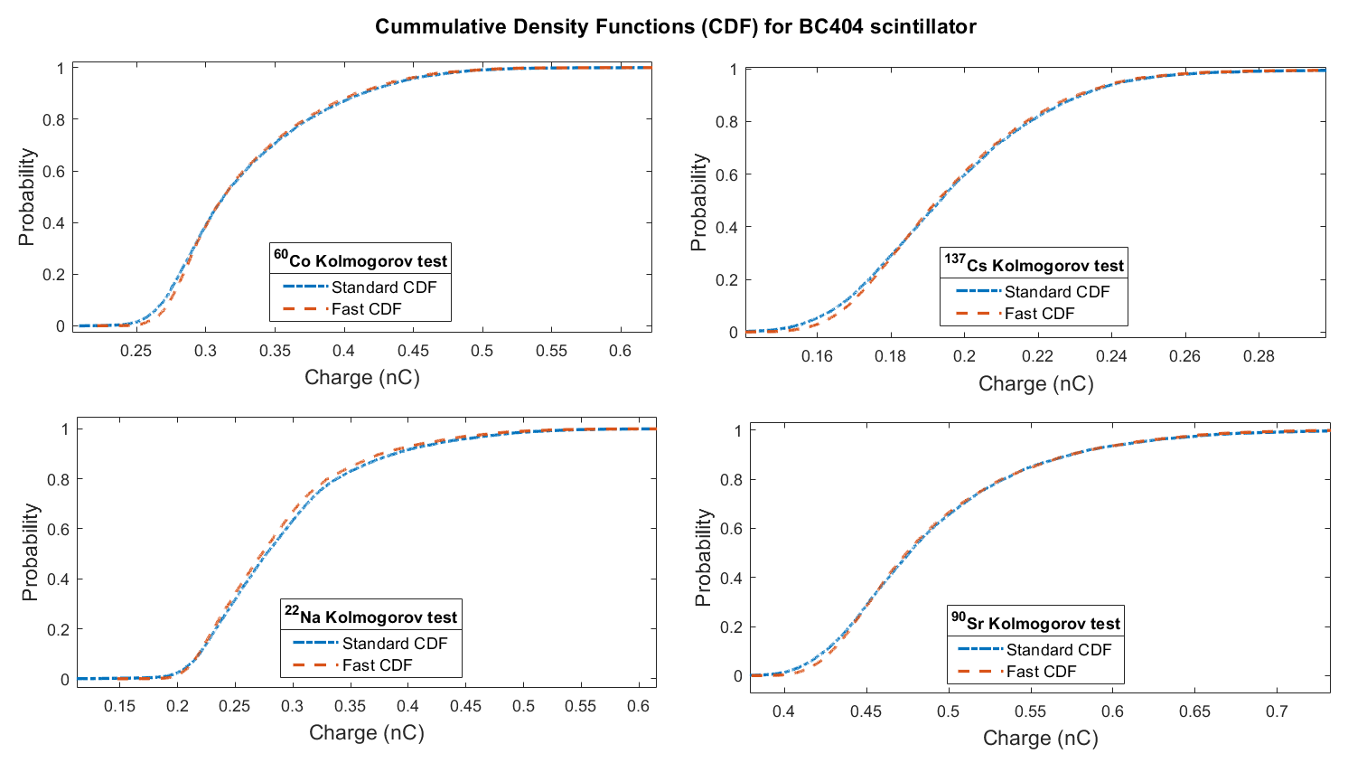
Figure 9: CDF comparative for BC404 scintillator.

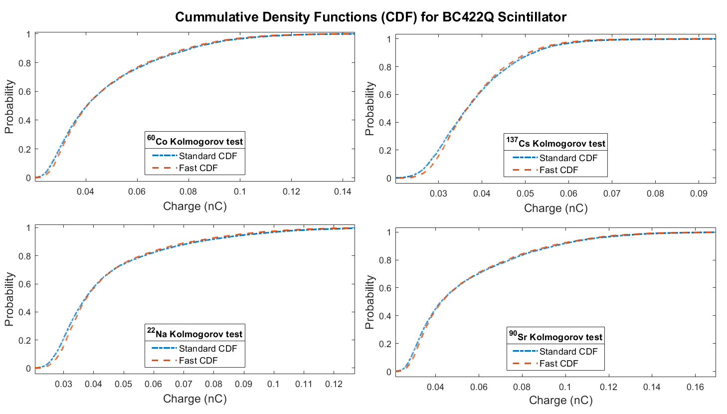
Figure 10: CDF comparative for BC422Q scintillator.

Table 12: Two-samples Kolmogorov test results for BC404 and BC422Q

-	BC404			BC422Q
Source	h	p	k	h	p	k
60Co	0	0.8172	0.0090	0	0.9609	0.0076
137Cs	0	0.9975	0.0057	0	0.9983	0.0060
22Na	0	1.0000	0.0044	0	0.9932	0.0066
90Sr	0	1.0000	0.0020	0	0.9901	0.0067

Additionally, the correlation between the mean and $\sigma$ values, obtained from our Gaussian fits for BC404 plastic scintillator material, can be used to distinguish among the different radiation sources used in this work. Accordingly with our results, this is not the case for BC422Q. (see Figure 11).

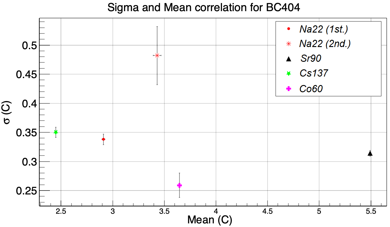
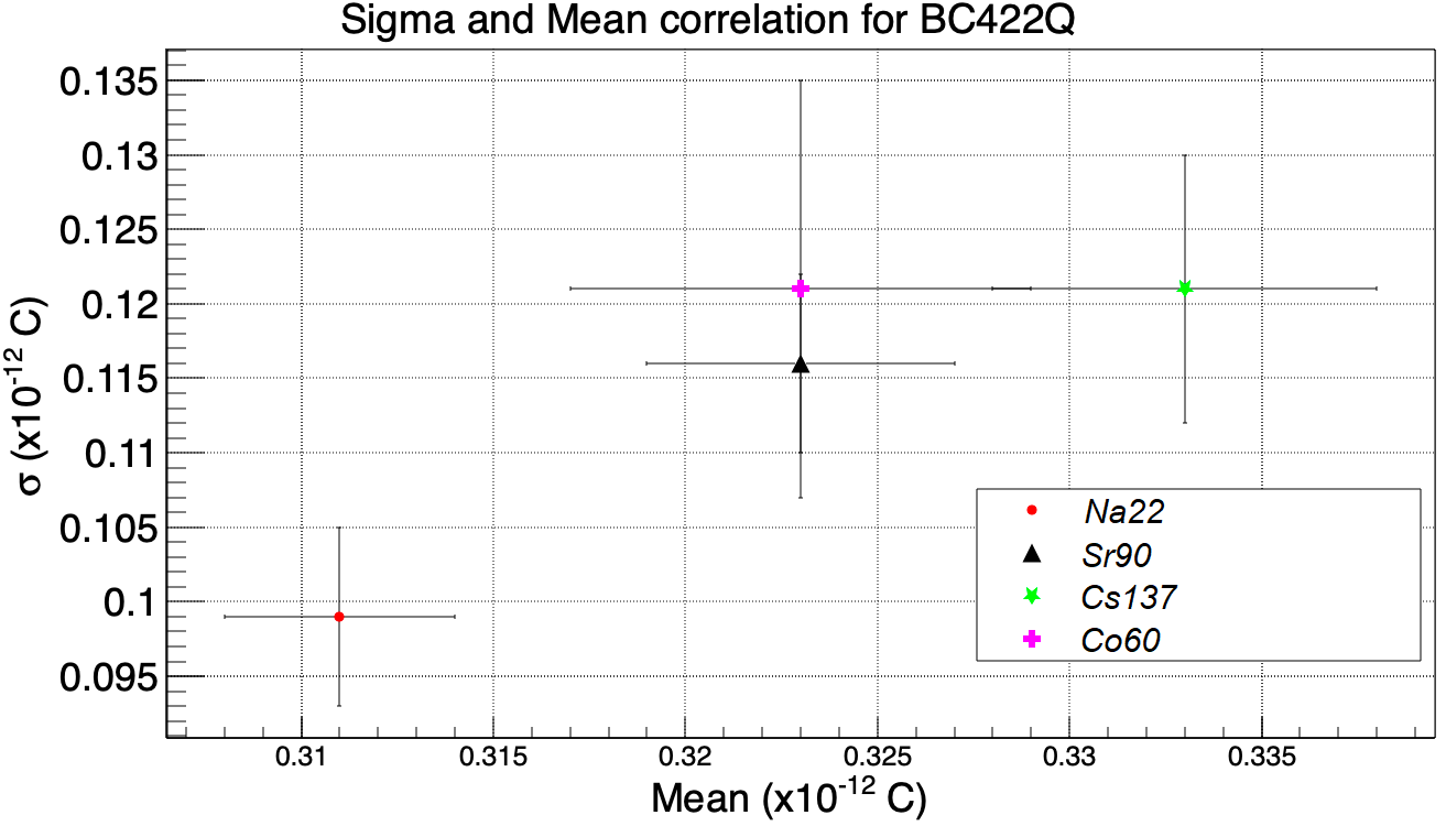
Figure 11: Mean-$\sigma$ relation from the Gaussian Fit for studied radiation sources with BC404 (up) and BC422Q (down) scintillators.

4 Conclusions

A relation between the fast and standard output signals of a SensL SiPM photo-sensor was found. For a given pulse, by using the fast output signal, we were able to reconstruct the deposited charge. This value is in good concordance with the estimated charge using the standard pulse. We also observed that the best agreement between the reconstructed charged from the fast output signal and the one from the standard output signal of a SensL SiPM photo-sensor is obtained for the BC422Q plastic scintillator. This results shows that it may be possible to develop a trigger system based on plastic scintillator material and a SensL SiPM photo-sensor with an excellent time resolution where also the information of electric charge can be reconstructed using the fast output signal of such photo-sensor.

In average, the conversion factor among fast and standard charge is $0.008\pm 0.001\times 10^{-12}$ for BC404 and $0.012\pm~{}0.001\times 10^{-12}$ for BC422Q. Whence, $Q_{S404}/Q_{F404}=128.205$ and $Q_{S422}/Q_{F422}=85.106$, which means that the charge deposition in the BC404 scintillator is 1.506 times the one for a BC422Q scintillator. Therefore (using these thin materials [11]), BC404 scintillator is 1.506 more sensitive than BC422Q scintillator for ⁹⁰Sr, ⁶⁰Co, ¹³⁷Cs and ²²Na radiation sources. This result gives the possibility to use the fast pulse from the detectors, where time resolution is an important restriction [17] and for fast triggering systems in Time of Flight (TOF) applications.
The continuity of this work is to estimate the time resolution of both detector configurations. Our plan is to develop a PET, commonly constructed with LYSO crystal, based on plastic scintillator materials with the best possible time resolution which is a key parameter during the data acquisition chain. For example, the life time of the isotopes used to acquire brain or heart images is around 2 minutes. Thus, a fast detector response is desired to improve the spatial and time resolution of PET scanners.

References

- [1] E. Garutti, Silicon photomultipliers for high energy physics detectors, J. Instrum. 6 (2011) 10 pg. C10003-C10003.
- [2] F. Simon, Silicon photomultipliers in particle and nuclear physics, NUCL INSTRUM METH A 926 (2019) pg. 85-100.
- [3] M. Pizzichemi et al., On light sharing TOF-PET modules with depth of interaction and 157 ps FWHM coincidence time resolution, Phys. Med. Biol 64 15 (2019) 15 pg. 155008.
- [4] E. Ebru and C. Celiktas, Effects of the positions of scintillation detectors with fast scintillators and photomultiplier tubes on TOF–PET performance, Pramana 94 (2020) 1.
- [5] W. Krzemien et al., A novel TOF-PET detector based on plastic scintillators, in 2015 IEEE Nuclear Science Symposium and Medical Imaging Conference (NSS/MIC), Octuber 2015.
- [6] L. Raczynski, Reconstruction of signal in plastic scintillator of PET using Tikhonov regularization, in 2015 37th Annual International Conference of the IEEE Engineering in Medicine and Biology Society (EMBC), August 2015.
- [7] A. Wieczorek et al., Novel scintillating material 2-(4-styrylphenyl)benzoxazole for the fully digital and MRI compatible J-PET tomograph based on plastic scintillators, PLoS One 12 (2017) 11 pg. e0186728.
- [8] K. O’Neil et al., SensL New Fast Timing SPM - High-Speed Silicon Photomultiplier Signal Output for High-Performance Timing Applications, doi: 10.22323/1.158.0022, May 2013 pg. 022.
- [9] SensL Technologies Ltd., Product Selection Guide, http://sensl.com/products 2013.
- [10] T. Cervi et al., Characterization of SiPM arrays in different series and parallel configurations, NUCL INSTRUM METH A 912 (2018) pg. 209-212.
- [11] E. Lamprou, Exploring TOF capabilities of PET detector blocks based on large monolithic crystals and analog SiPMs, PHYS MEDICA 70 (2020) pg. 10-18.
- [12] M. Nemallapudi , Single photon time resolution of state of the art SiPMs, J INSTRUM 11 (2016) 10.
- [13] K. Kuper, On reachable energy resolution of SiPM based scintillation counters for X-ray detection, J INSTRUM 12 (2017) 01 pg. P01001-P01001.
- [14] P. Lv, A low-energy sensitive compact gamma-ray detector based on LaBr <sub>3</sub> and SiPM for GECAM, J INSTRUM 13 (2018) 08 pg. P08014-P08014.
- [15] Y. Junhao, Pulse shape discrimination based on fast signals from silicon photomultipliers, NUCL INSTRUM METH A 894 (2018) pg. 129-137.
- [16] D. Sergei, Timing resolution performance comparison for fast and standard outputs of SensL SiPM, IEEE Nuclear Science Symposium Conference Record (2013).
- [17] M. Alvarado et al., A beam–beam monitoring detector for the MPD experiment at NICA, NUCL INSTRUM METH A 953 (2020) pg. 163150.
- [18] CRYSTALS SAINT-GOBAIN BC400 BC404 BC408 BC412 BC416 Data Sheet (2005–2018)
- [19] CRYSTALS SAINT-GOBAIN BC22Q Data Sheet (2005–2016)
- [20] AMCRYS, Plastic Scintillators for n and gamma discrimination, http://www.amcrys.com/details.html?cat_id=146&id=4302.
- [21] R. Brun, ROOT — An object oriented data analysis framework, NUCL INSTRUM METH A 389 (1997) 1-2 pg.81-86.
- [22] Ma. Rubao, Asymptotic Properties of Pearson’s Rank-Variate Correlation Coefficient under Contaminated Gaussian Model, PLoS One 9 (2014) 11 pg. 1-15.
- [23] A. Papoullis and S.U. Pillai. Probability, Random Variables and Stochastic Processes. McGraw-Hill, Series in electrical engineering: Communications and Signal Processsing. McGarw-Hill, 2002.
- [24] Motulsky, H. Christopoulos, A. Fitting models for biological data using linear and non linear regression: A practical guide to curve fitting. Oxford University Press, 2004.
- [25] Stephen W. Looney, Joseph L. Hagan. Statistical Methods for Assessing Biomarkers and Analyzing Biomarker Data. C.R. Rao, J.P. Miller, D.C. Rao, Essential Statistical Methods for Medical Statistics, North-Holland, 2011, Pages 27-65, ISBN 9780444537379,
- [26] Hassani, H.; Silva, E.S. A Kolmogorov-Smirnov Based Test for Comparing the Predictive Accuracy of Two Sets of Forecasts. Econometrics 2015, 3, 590-609.
- [27] Mukhopadhyay, S. Sun . "Plastic Gamma Sensors: An Application in Detection of Radioisotopes". United States. https://www.osti.gov/servlets/purl/811396