Equilibrium Validation in Models for Pattern Formation Based on Sobolev Embeddings

Abstract.

In the study of equilibrium solutions for partial differential equations there are so many equilibria that one cannot hope to find them all. Therefore one usually concentrates on finding individual branches of equilibrium solutions. On the one hand, a rigorous theoretical understanding of these branches is ideal but not generally tractable. On the other hand, numerical bifurcation searches are useful but not guaranteed to give an accurate structure, in that they could miss a portion of a branch or find a spurious branch where none exists. In a series of recent papers, we have aimed for a third option. Namely, we have developed a method of computer-assisted proofs to prove both existence and isolation of branches of equilibrium solutions. In the current paper, we extend these techniques to the Ohta-Kawasaki model for the dynamics of diblock copolymers in dimensions one, two, and three, by giving a detailed description of the analytical underpinnings of the method. Although the paper concentrates on applying the method to the Ohta-Kawasaki model, the functional analytic approach and techniques can be generalized to other parabolic partial differential equations.

1. Introduction

The goal of this paper is to present the theoretical underpinnings for computer-assisted branch validation using functional analytic techniques including the constructive implicit function theorem and Neumann series methods, such that pointwise estimates result in solution branch validation. While the individual proof techniques presented here are not novel, we present this approach in a modular way such that it is flexible, adaptable, and as computationally feasible as possible in more than one space dimension. In particular, we apply this methodology in the case of the Ohta–Kawasaki model for diblock copolymers [24]. Diblock copolymers are formed by the chemical reaction of two linear polymers (known as blocks) which contain different monomers. Whenever the blocks are thermodynamically incompatible, the blocks are forced to separate after the reaction, but since the blocks are covalently bonded they cannot separate on a macroscopic scale. The competition between these long-range and short-range forces causes microphase separation, resulting in pattern formation on a mesoscopic scale.

We study the Ohta-Kawasaki equation in the case of homogeneous Neumann boundary conditions on rectilinear domains $\Omega$ in dimensions one, two, and three, which is given by

$$w_{t} = -\Delta(\Delta w+\lambda f(w))-\lambda\sigma(w-\mu)\quad\mbox{ in }\Omega\;,$$

$$\frac{\partial w}{\partial\nu}=\frac{\partial(\Delta w)}{\partial\nu}=0\quad\mbox{ on }\partial\Omega\;.$$

The notation $\nu$ denotes the unit outward normal on the boundary of $\Omega$ — corresponding to homogeneous Neumann boundary conditions. The quantity $w(t,x)$ is the local average density of the two blocks. The parameter $\mu$ is the space average of $w$, meaning it is a measure of the relative total proportion of the two polymers, which we tersely refer to as the mass of the system. The equation obeys a mass conservation, implying that $\mu$ is time-invariant. A large value of parameter $\lambda$ corresponds to a large short-range repulsion, while a large value of the parameter $\sigma$ corresponds to large long-range elasticity forces. We refer the reader to [16] for a detailed description of how $\lambda$ and $\sigma$ are defined. The nonlinear function $f:{\mathbb{R}}\to{\mathbb{R}}$ is often assumed to be $f(u)=u-u^{3}$, but the results in this paper still apply as long as $f$ is a $C^{2}$-function. Finally, note that the second boundary condition is necessary since this is a fourth order equation. In this paper, we focus on equilibrium solutions $w=w(x)$.

For notational convenience, we reformulate our equation slightly. For a solution $w$ of the diblock copolymer equation, we define $u=w-\mu$. Since the space average of $w$ is $\mu$, the average of the shifted function $u$ is zero. Therefore the equilibrium equation becomes

$$-\Delta(\Delta u+\lambda f(u+\mu))-\lambda\sigma u = 0\quad\mbox{ in }\Omega\;,$$

(1) $$\frac{\partial u}{\partial\nu}=\frac{\partial(\Delta u)}{\partial\nu} = 0\quad\mbox{ on }\partial\Omega\;,$$

$$\int_{\Omega}u\;dx = 0\;.$$

We will use this version of the equation for the rest of the paper. We focus on solutions to this equation as we vary any of the three parameters: the degree of short-range repulsion $\lambda$, the mass $\mu$, and the degree of long-range elasticity $\sigma$. Our main goal is to establish bounds that make it possible to use a functional analytic approach to rigorous validation using the point of view of the constructive implicit function theorem which we have already developed in previous work [30, 35, 36, 37]. Our bounds are developed mostly using theoretical techniques, but in the case of Sobolev embeddings, the bounds themselves are developed using computer-assisted means. This method is designed for validated continuation of branches of solutions which depend on a parameter, in the spirit of the numerical method of pseudo-arclength continuation, such as seen in the software packages AUTO [13] and Matcont [12]. Successive application of this theorem allows us to validate branches of equilibrium solutions by giving precise bounds on both the branch approximation error and isolation. This is much more powerful than only validating individual solutions along a branch, since it allows us to guarantee that a set of solutions lie along the same connected branch component.

In order to establish what is new in this paper, we give a brief discussion of previous results. A number of papers have previously considered numerical computation of bifurcation diagrams for the Ohta-Kawasaki and Cahn-Hilliard equations, such as for example [5, 6, 7, 8, 11, 16, 19, 20]. There are also several decades of results on computer validation for dynamical systems and differential equations solutions which combine fixed point arguments and interval arithmetic; see for example [2, 10, 14, 25, 26, 27, 29, 35, 36]. A constructive implicit function theorem was formulated in the work of Chierchia [4]. Our approach follows most closely the work of Plum [23, 25, 26, 27], in which functional analytic approaches are given for establishing needed apriori bounds. Such methods have also been applied by Yamamoto [41, 42]. In our previous work on the constructive implicit function theorem, our goal has been to give a systematic procedure for adapting these works to the context of parameter continuation. There are several papers that have already considered rigorous validation of parameter-dependent solutions for the Ohta-Kawasaki model [3, 9, 18, 30, 32, 33, 34, 35, 36, 37]. Many of these papers also include methods of bounding the terms in a generalized Fourier series, and the estimates on the tail. However, it was necessary to make quite substantial ad hoc calculations in order to establish needed bounds before it is possible to proceed with numerical validation.

Our goal in the current paper is to establish a set of flexible bounds on the size of the inverse of the derivative, the required truncation dimension, Lipschitz bounds on the equations with respect to all parameters, as well as constructive Sobolev embedding constant bounds for comparison to the $L^{\infty}$-norm, meaning that equilibrium verifications along branch segments can be done without having to resort to ad hoc calculations which crucially depend on the specific nonlinearity. More precisely, we obtain the following:

• The approach of this paper derives general estimates that work in one, two, and three space dimensions, and under the natural homogeneous Neumann boundary conditions. This is in contrast to [3] and [36], which only considered the case of one-dimensional domains, or to [33, 34], which considered the three-dimensional case only under periodic boundary conditions and symmetry constraints.

• Our approach uses the natural functional analytic setting for the diblock copolymer evolution equation, which is based on the Sobolev space of twice weakly differentiable functions. This is in contrast to [33, 34], which seek the equilibria in spaces of analytic functions.

• As part of our approach, we obtain accurate upper bounds for the operator norm of the inverse of the diblock copolymer Fréchet derivative. For this estimate, we use the natural Sobolev norms of the underlying problem. In contrast to [17, 39, 40] our method is based on Neumann series.

Throughout this paper, we focus on the theoretical underpinnings which allow one to apply the constructive implicit function theorem [30]. Due to space constraints, we leave the practical application of these results to path-following with slanted boxes as in [30], as well as extensions to pseudo-arclength continuation, for future work. Nevertheless, while this paper is focussed only on the Ohta-Kawasaki model, the general approach can be used for other parabolic partial differential equations as well.

The remainder of this paper is organized as follows. In Section 2, we introduce the necessary functional analytic framework, while Section 3 is devoted to finding bounds on the operator norm of the inverse of the linearized operator. After that, Section 4 establishes Lipschitz bounds on the diblock copolymer operator for continuation with respect to any of the three parameters $\lambda$, $\sigma$, and $\mu$, before in Section 5 we give a brief numerical illustration of how this method rigorously establishes a variety of equilibrium branch pieces for the Ohta-Kawasaki model in multiple dimensions. Finally, in Section 6 we wrap up with conclusions and future plans.

2. Basic definitions and setup

In this section, we establish notation and crucial auxiliary bounds. In Section 2.1 we recall the constructive implicit function theorem, before in Section 2.2 we define the function spaces that will be used in our computer-assisted proofs. These spaces are particularly adapted for the use with Fourier series expansions to represent functions with Neumann boundary conditions and zero average. In Section 2.3, we collect a set of Sobolev embedding results giving precise rigorous bounds on the similarity constants for passing between equivalent norms on these function spaces. Finally, in Section 2.4 we introduce the necessary finite-dimensional spaces and associated projection operators that are used in our computer-assisted proofs.

2.1. The constructive implicit function theorem

In this section we state a constructive implicit function theorem that makes it possible to validate a branch of solutions changing with respect to a parameter. This theorem appears in [30], where we demonstrated the validation of solutions for the lattice Allen-Cahn equation. The theorem is based on previous work of Plum [27] and Wanner [36]. To put this in context, our overarching goal is to find a connected curve of values $(\alpha,x)$ in the zero set for a specific nonlinear operator ${\mathcal{G}}(\alpha,x)$. In this paper, the zero set consists of the equilibria of the Ohta-Kawasaki equation. Starting at a point for which the operator ${\mathcal{G}}$ is close to zero, we use the theorem as the iterative step in a validated continuation. That is, we iteratively validate small portions along the solution curve, each time using the constructive implicit function theorem which is stated below. We also validate that these portions combine to create a piece of a single connected solution curve, and show that it is isolated from any other branch of the solution curve. Rather than getting bogged down in the details of the iterative process, we first concentrate on the single iterative step and the estimates needed in order to perform it. Specifically, we consider solutions to the equation

(2) $${\mathcal{G}}(\alpha,x)=0\;,$$

where ${\mathcal{G}}:{\mathcal{P}}\times{\mathcal{X}}\to{\mathcal{Y}}$ is a Fréchet differentiable nonlinear operator between two Banach spaces ${\mathcal{X}}$ and ${\mathcal{Y}}$, and the parameter $\alpha$ is taken from a Banach space ${\mathcal{P}}$. The norms on these Banach spaces are denoted by $\|\cdot\|_{\mathcal{P}}$, $\|\cdot\|_{\mathcal{X}}$, and $\|\cdot\|_{\mathcal{Y}}$, respectively. One possible choice of ${\mathcal{G}}$ would be to directly use the nonlinear operator associated with (1), but this is not a numerically viable option for validation of a branch of solutions. Instead we will introduce an extended system which gives a validated version of pseudo-arclength continuation. The system contains not only the Ohta-Kawasaki model equilibrium equation, but is in a way designed to optimize the needed number of validation steps.

In order to present the constructive implicit function theorem in detail, we begin by making the following hypotheses. For the classical implicit function theorem, the existence of constants satisfying the hypotheses given below is sufficient. In contrast, since we wish to use a computer assisted proof to validate existence of equilibria with specified error bounds, we require explicit values for each of the constants in (H1)–(H4).

• Unlike the traditional implicit function theorem, we assume only an approximate solution to the equation. That is, assume that we are given a pair $(\alpha^{*},x^{*})\in{\mathcal{P}}\times{\mathcal{X}}$ which is an approximate solution of the nonlinear problem (2). More precisely, the residual of the nonlinear operator ${\mathcal{G}}$ at the pair $(\alpha^{*},x^{*})$ is small, i.e., there exists a constant $\varrho>0$ such that

  $$\left\|{\mathcal{G}}(\alpha^{*},x^{*})\right\|_{\mathcal{Y}}\leq\varrho\;.$$

• Assume that the operator $D_{x}{\mathcal{G}}(\alpha^{*},x^{*})$ is invertible and not very close to being singular. That is, the Fréchet derivative $D_{x}{\mathcal{G}}(\alpha^{*},x^{*})\in{\mathcal{L}}({\mathcal{X}},{\mathcal{Y}})$, where ${\mathcal{L}}({\mathcal{X}},{\mathcal{Y}})$ denotes the Banach space of all bounded linear operators from ${\mathcal{X}}$ into ${\mathcal{Y}}$, is one-to-one and onto, and its inverse $D_{x}{\mathcal{G}}(\alpha^{*},x^{*})^{-1}:{\mathcal{Y}}\to{\mathcal{X}}$ is bounded and satisfies

  $$\left\|D_{x}{\mathcal{G}}(\alpha^{*},x^{*})^{-1}\right\|_{{\mathcal{L}}({\mathcal{Y}},{\mathcal{X}})}\leq K\;,$$

  where $\|\cdot\|_{{\mathcal{L}}({\mathcal{Y}},{\mathcal{X}})}$ denotes the operator norm in ${\mathcal{L}}({\mathcal{Y}},{\mathcal{X}})$.

• For $(\alpha,x)$ close to $(\alpha^{*},x^{*})$, the Fréchet derivative $D_{x}{\mathcal{G}}(\alpha,x)$ is locally Lipschitz continuous in the following sense. There exist positive real constants $L_{1}$, $L_{2}$, $\ell_{x}$, and $\ell_{\alpha}\geq 0$ such that for all pairs $(\alpha,x)\in{\mathcal{P}}\times{\mathcal{X}}$ with $\|x-x^{*}\|_{\mathcal{X}}\leq\ell_{x}$ and $\|\alpha-\alpha^{*}\|_{\mathcal{P}}\leq\ell_{\alpha}$ we have

  $$\left\|D_{x}{\mathcal{G}}(\alpha,x)-D_{x}{\mathcal{G}}(\alpha^{*},x^{*})\right\|_{{\mathcal{L}}({\mathcal{X}},{\mathcal{Y}})}\leq L_{1}\left\|x-x^{*}\right\|_{\mathcal{X}}+L_{2}\left\|\alpha-\alpha^{*}\right\|_{\mathcal{P}}\;.$$

  To verify this condition, as well as the next one, we will give specific Lipschitz bounds on the Ohta-Kawasaki operator. We will then show the precise way to combine these bounds in order to get the constants $L_{k}$.

• For $\alpha$ close to $\alpha^{*}$, the Fréchet derivative $D_{\alpha}{\mathcal{G}}(\alpha,x^{*})$ satisfies a Lipschitz-type bound. More precisely, there exist positive real constants $L_{3}$ and $L_{4}$, such that for all $\alpha\in{\mathcal{P}}$ with $\|\alpha-\alpha^{*}\|_{\mathcal{P}}\leq\ell_{\alpha}$ one has

  $$\left\|D_{\alpha}{\mathcal{G}}(\alpha,x^{*})\right\|_{{\mathcal{L}}({\mathcal{P}},{\mathcal{Y}})}\leq L_{3}+L_{4}\left\|\alpha-\alpha^{*}\right\|_{\mathcal{P}}\;,$$

  where $\ell_{\alpha}$ is the constant that was chosen in (H3).

Keeping these hypotheses in mind, the constructive implicit function theorem can then be stated as follows.

Theorem 2.1 (Constructive Implicit Function Theorem).

Let ${\mathcal{P}}$, ${\mathcal{X}}$, and ${\mathcal{Y}}$ be Banach spaces, suppose that the nonlinear operator ${\mathcal{G}}:{\mathcal{P}}\times{\mathcal{X}}\to{\mathcal{Y}}$ is Fréchet differentiable, and assume that the pair $(\alpha^{*},x^{*})\in{\mathcal{P}}\times{\mathcal{X}}$ satisfies hypotheses (H1), (H2), (H3), and (H4). Finally, suppose that

(3) $$4K^{2}\varrho L_{1}<1\qquad\mbox{ and }\qquad 2K\varrho<\ell_{x}\;.$$

Then there exist pairs of constants $(\delta_{\alpha},\delta_{x})$ with $0\leq\delta_{\alpha}\leq\ell_{\alpha}$ and $0<\delta_{x}\leq\ell_{x}$, as well as

(4) $$2KL_{1}\delta_{x}+2KL_{2}\delta_{\alpha}\leq 1\qquad\mbox{ and }\qquad 2K\varrho+2KL_{3}\delta_{\alpha}+2KL_{4}\delta_{\alpha}^{2}\leq\delta_{x}\;,$$

and for each such pair the following holds. For every $\alpha\in{\mathcal{P}}$ with $\|\alpha-\alpha^{*}\|_{\mathcal{P}}\leq\delta_{\alpha}$ there exists a uniquely determined element $x(\alpha)\in{\mathcal{X}}$ with $\|x(\alpha)-x^{*}\|_{\mathcal{X}}\leq\delta_{x}$ such that ${\mathcal{G}}(\alpha,x(\alpha))=0$. In other words, if we define

$${\mathcal{B}}_{\delta}^{\mathcal{X}}=\left\{\xi\in{\mathcal{X}}\;:\;\left\|\xi-x^{*}\right\|_{\mathcal{X}}\leq\delta\right\}\quad\mbox{ and }\quad{\mathcal{B}}_{\delta}^{\mathcal{P}}=\left\{p\in{\mathcal{P}}\;:\;\left\|p-\alpha^{*}\right\|_{\mathcal{P}}\leq\delta\right\}\;,$$

then all solutions of the nonlinear problem ${\mathcal{G}}(\alpha,x)=0$ in the set ${\mathcal{B}}_{\delta_{\alpha}}^{\mathcal{P}}\times{\mathcal{B}}_{\delta_{x}}^{\mathcal{X}}$ lie on the graph of the function $\alpha\mapsto x(\alpha)$. In addition, the following two statements are satisfied.

• For all pairs $(\alpha,x)\in{\mathcal{B}}_{\delta_{\alpha}}^{\mathcal{P}}\times{\mathcal{B}}_{\delta_{x}}^{\mathcal{X}}$ the Fréchet derivative $D_{x}{\mathcal{G}}(\alpha,x)\in{\mathcal{L}}({\mathcal{X}},{\mathcal{Y}})$ is a bounded invertible linear operator, whose inverse is in ${\mathcal{L}}({\mathcal{Y}},{\mathcal{X}})$.

• If the mapping ${\mathcal{G}}:{\mathcal{P}}\times{\mathcal{X}}\to{\mathcal{Y}}$ is $k$-times continuously Fréchet differentiable, then so is the solution function $\alpha\mapsto x(\alpha)$.

Throughout the remainder of this paper, we concentrate on finding computationally accessible versions of hypotheses (H2), (H3), and (H4) for the Ohta-Kawasaki model.

2.2. Function spaces

Throughout this paper, we let $\Omega=(0,1)^{d}$ denote the unit cube in dimension $d=1,2,3$, and define the constants

$$c_{0}=1\quad\mbox{ and }\quad c_{\ell}=\sqrt{2}\quad\mbox{ for }\quad\ell\in{\mathbb{N}}\;.$$

If $k\in{\mathbb{N}}_{0}^{d}$ denotes an arbitrary multi-index of the form $k=(k_{1},\dots,k_{d})$, then let

$$c_{k}=c_{k_{1}}\cdot\ldots\cdot c_{k_{d}}\;.$$

If we then define

(5) $$\varphi_{k}(x)=c_{k}\prod_{i=1}^{d}\cos(k_{i}\pi x_{i})\quad\mbox{ for all }\quad x=(x_{1},\ldots,x_{d})\in\Omega\;,$$

then the function collection $\{\varphi_{k}\}_{k\in{\mathbb{N}}_{0}^{d}}$ forms a complete orthonormal basis for the space $L^{2}(\Omega)$. Any measurable and square-integrable function $u:\Omega\to{\mathbb{R}}$ can be written in terms of its Fourier cosine series

(6) $$u(x)=\sum_{k\in{\mathbb{N}}_{0}^{d}}\alpha_{k}\varphi_{k}(x)\;,$$

where $\alpha_{k}\in{\mathbb{R}}$ are the Fourier coefficients of $u$. Finally, we define

$$|k|=(k_{1}^{2}+\dots+k_{d}^{2})^{1/2}\quad\mbox{ and }\quad|k|_{\infty}=\max(k_{1},\dots,k_{d})\;.$$

Each function $\varphi_{k}(x)$ is an eigenfunction of the negative Laplacian. The corresponding eigenvalue is given by $\kappa_{k}$, defined via the equation

$$-\Delta\varphi_{k}(x)=\kappa_{k}\varphi_{k}(x)\qquad\mbox{ with }\qquad\kappa_{k}=\pi^{2}\left(k_{1}^{2}+k_{2}^{2}+\dots+k_{d}^{2}\right)=\pi^{2}|k|^{2}\;.$$

A straightforward direct computation shows that each $\varphi_{k}(x)$ satisfies the homogeneous Neumann boundary condition $\partial\varphi_{k}/\partial\nu=0$. In addition, as a result of being an eigenfunction of $-\Delta$, each function $\varphi_{k}(x)$ also satisfies the second boundary condition in (1), since the identity $\partial(\Delta\varphi_{k})/\partial\nu=-\kappa_{k}\partial\varphi_{k}/\partial\nu=0$ holds. Therefore any finite Fourier series as above automatically satisfies both boundary conditions of the diblock copolymer equation.

Based on our construction, the family $\{\varphi_{k}\}_{k\in{\mathbb{N}}_{0}^{d}}$ is a complete orthonormal basis for the space $L^{2}(\Omega)$. Thus, if $u$ is given as in (6) one can easily see that

$$\|u\|_{L^{2}}=\left(\sum_{k\in{\mathbb{N}}_{0}^{d}}\alpha_{k}^{2}\right)^{1/2}\;.$$

For our application to the diblock copolymer model, we need to work with suitable subspaces of the Sobolev spaces $H^{k}(\Omega)=W^{k,2}(\Omega)$, see for example [1]. These subspaces have to reflect the required homogeneous Neumann boundary conditions and they can be introduced as follows. For $\ell\in{\mathbb{N}}$ consider the space

$${\mathcal{H}}^{\ell}=\left\{u=\sum_{k\in{\mathbb{N}}_{0}^{d}}\alpha_{k}\varphi_{k}:\|u\|_{{\mathcal{H}}^{\ell}}<\infty\right\}\;,$$

where

$$\|u\|_{{\mathcal{H}}^{\ell}}=\left(\sum_{k\in{\mathbb{N}}_{0}^{d}}\left(1+\kappa_{k}^{\ell}\right)\alpha_{k}^{2}\right)^{1/2}\;.$$

One can easily verify that this is equivalent to the definition

$$\|u\|^{2}_{{\mathcal{H}}^{\ell}}=\|u\|_{L^{2}}^{2}+\left\|(-\Delta)^{\ell/2}u\right\|^{2}_{L^{2}}\;,$$

where $\|\cdot\|_{L^{2}}$ denotes the standard $L^{2}(\Omega)$-norm on the domain $\Omega$ as mentioned above, and the fractional Laplacian for odd $\ell$ is defined using the spectral definition. We note that we have incorporated the boundary conditions of (1) into our definition of the spaces ${\mathcal{H}}^{\ell}$. For example,

$${\mathcal{H}}^{1} = H^{1}(\Omega),$$

$${\mathcal{H}}^{2} = \left\{u\in H^{2}(\Omega):\frac{\partial u}{\partial\nu}=0\right\}\,\quad\mbox{, and }$$

$${\mathcal{H}}^{4} = \left\{u\in H^{4}(\Omega):\frac{\partial u}{\partial\nu}=\frac{\partial\Delta u}{\partial\nu}=0\right\}\,,$$

where the boundary conditions in the second and third equations are considered in the sense of the trace operator. The first identity follows as a special case from the results in [15, 22], the second identity has been established in [21, Lemma 3.2], and also the third identity can be verified as in [21, Lemma 3.2]. For the sake of simplicity we further define ${\mathcal{H}}^{0}=L^{2}(\Omega)$.

While the spaces ${\mathcal{H}}^{\ell}$ incorporate the boundary conditions of (1), recall that we have reformulated the diblock copolymer equation in such a way that solutions satisfy the integral constraint $\int_{\Omega}u\;dx=0$, since the case of nonzero average has been absorbed into the placement of the parameter $\mu$. In order to treat this additional constraint, we therefore need to restrict the spaces ${\mathcal{H}}^{\ell}$ further. Consider now an arbitrary integer $\ell\in{\mathbb{Z}}$ and define the space

(7) $$\overline{{\mathcal{H}}}^{\ell}=\left\{u=\sum_{k\in{\mathbb{N}}_{0}^{d},\;|k|>0}\alpha_{k}\varphi_{k}\;:\;\|u\|_{\overline{{\mathcal{H}}}^{\ell}}<\infty\right\}\;,$$

where we use the modified norm

(8) $$\|u\|_{\overline{{\mathcal{H}}}^{\ell}}=\left(\sum_{k\in{\mathbb{N}}_{0}^{d},\;|k|>0}\kappa_{k}^{\ell}\alpha_{k}^{2}\right)^{1/2}\;.$$

Notice that for $\ell=0$ this definition reduces to the subspace of $L^{2}(\Omega)$ of all functions with average zero equipped with its standard norm, since we removed the constant basis function from the Fourier series. For $\ell>0$ one can easily see that $\overline{{\mathcal{H}}}^{\ell}\subset{\mathcal{H}}^{\ell}$, and that the new norm is equivalent to our norm on ${\mathcal{H}}^{\ell}$. We still need to shed some light on the new definition (7) for negative integers $\ell<0$. In this case, the series in (6) is interpreted formally, i.e., the element $u\in\overline{{\mathcal{H}}}^{\ell}$ for $\ell<0$ is identified with the sequence of its Fourier coefficients. Moreover, one can easily see that in this case $u$ acts as a bounded linear functional on $\overline{{\mathcal{H}}}^{-\ell}$. In fact, for all $\ell<0$ the space $\overline{{\mathcal{H}}}^{\ell}$ can be considered as a subspace of the negative exponent Sobolev space $H^{\ell}(\Omega)=W^{\ell,2}(\Omega)$, see again [1]. Finally, for every $\ell\in{\mathbb{Z}}$ the space $\overline{{\mathcal{H}}}^{\ell}$ is a Hilbert space with inner product

$$(u,v)_{\overline{{\mathcal{H}}}^{\ell}}=\sum_{k\in{\mathbb{N}}_{0}^{d},\;|k|>0}\kappa_{k}^{\ell}\alpha_{k}\beta_{k}\;,$$

where

$$u=\sum_{k\in{\mathbb{N}}_{0}^{d},\;|k|>0}\alpha_{k}\varphi_{k}\in\overline{{\mathcal{H}}}^{\ell}\qquad\mbox{ and }\qquad v=\sum_{k\in{\mathbb{N}}_{0}^{d},\;|k|>0}\beta_{k}\varphi_{k}\in\overline{{\mathcal{H}}}^{\ell}\;.$$

The above spaces form the functional analytic backbone of this paper, and they allow us to reformulate the equilibrium problem for (1) as a zero finding problem. Note first, however, that the functions $\varphi_{k}$ can also be used to obtain an orthonormal basis in $\overline{{\mathcal{H}}}^{\ell}$. In fact, we only have to drop the constant function $\varphi_{0}$ and apply the following rescaling.

Lemma 2.2.

The set $\left\{\kappa_{k}^{-\ell/2}\varphi_{k}(x)\right\}_{k\in{\mathbb{N}}_{0}^{d},\;|k|>0}$ forms a complete orthonormal set for the Hilbert space $\overline{{\mathcal{H}}}^{\ell}$.

We close this section by briefly showing how the diblock copolymer equilibrium problem can be stated as a zero set problem in our functional analytic setting. For this, consider the operator

$$F:{\mathbb{R}}^{3}\times X\to Y\;,\qquad\mbox{ with }\qquad X=\overline{{\mathcal{H}}}^{2}\quad\mbox{ and }\quad Y=\overline{{\mathcal{H}}}^{-2}\;,$$

which is defined as

(9) $$F(\lambda,\sigma,\mu,u)=-\Delta\left(\Delta u+\lambda f(u+\mu)\right)-\lambda\sigma u\;.$$

The problem is now formulated weakly, and in particular, the second boundary condition $\partial(\Delta u)/\partial\nu=0$ is no longer explicitly stated in this weak formulation. Note, however, that the first boundary condition $\partial u/\partial\nu=0$ has been incorporated into the space $X=\overline{{\mathcal{H}}}^{2}$. The fact that $f$ is $C^{2}$ is sufficient to guarantee that the function $F$ maps $X$ to $Y$, since we only consider domains up to dimension three. Then for fixed parameters, an equilibrium solution $u$ to the diblock copolymer equation (1) is a function which satisfies the identity $F(\lambda,\sigma,\mu,u)=0$. Moreover, the Fréchet derivative of the operator $F$ with respect to $u$ at this equilibrium is given by

(10) $$D_{u}F(\lambda,\sigma,\mu,u)[v]=-\Delta\left(\Delta v+\lambda f^{\prime}(u+\mu)v\right)-\lambda\sigma v\;.$$

In our formulation, the boundary and integral conditions which are part of (1) have been incorporated into the choice of the domain $X=\overline{{\mathcal{H}}}^{2}$ of the nonlinear operator $F$.

2.3. Constructive Sobolev embedding and Banach algebra constants

For classical Sobolev embedding theorems, it is sufficient to write statements such as “the Sobolev space ${\mathcal{H}}^{2}$ can be continuously embedded into $L^{\infty}(\Omega)$,” without worrying about the specific constants needed to do so. However, for the purpose of computer-assisted proofs, such statements are insufficient. Instead we need specific numerical bounds to compare the norms of a function or product of functions when considered in different spaces. Parallel to the name constructive implicit function theorem, we refer to the bounds on the constants as constructive Sobolev embedding constants. In addition, we will need a constructive Banach algebra estimate on the relationship between $\|uv\|_{{\mathcal{H}}^{2}}$ and the product $\|u\|_{{\mathcal{H}}^{2}}\|v\|_{{\mathcal{H}}^{2}}$. In particular, we require the exact values of $C_{m}$, $\overline{C}_{m}$, and $C_{b}$ in one, two, and three dimensions given in the following equations:

$$\|u\|_{\infty} \leq C_{m}\;\|u\|_{{\mathcal{H}}^{2}}\;,\qquad\qquad\mbox{ for all }u\in{\mathcal{H}}^{2}\;,$$

(11) $$\|u\|_{\infty} \leq \overline{C}_{m}\;\|u\|_{\overline{{\mathcal{H}}}^{2}}\;,\qquad\qquad\mbox{ for all }u\in\overline{{\mathcal{H}}}^{2}\;,$$

$$\|uv\|_{{\mathcal{H}}^{2}} \leq C_{b}\;\|u\|_{{\mathcal{H}}^{2}}\|v\|_{{\mathcal{H}}^{2}}\;,\quad\;\;\;\mbox{ for all }u,v\in{\mathcal{H}}^{2}\;.$$

The values of $C_{m}$ and $C_{b}$ in dimensions $1$, $2$, and $3$ were established in [38] using rigorous computational techniques. The values of $\overline{C}_{m}$ can be obtained by adapting the approach in this paper, as outlined in the next lemma. Table 1 summarizes the values of all necessary constants.

Dimension $d$	$1$	$2$	$3$
Sobolev Embedding Constant $C_{m}$	$1.010947$	$1.030255$	$1.081202$
Sobolev Embedding Constant $\overline{C}_{m}$	$0.149072$	$0.248740$	$0.411972$
Banach Algebra Constant $C_{b}$	$1.471443$	$1.488231$	$1.554916$

Table 1. These values are rigorous upper bounds for the embedding constants in (11).

Lemma 2.3 (Sobolev embedding for the zero mass case).

For all functions $u\in\overline{{\mathcal{H}}}^{2}$ we have the estimate

(12) $$\|u\|_{\infty}\quad\leq\quad\|u\|_{\overline{{\mathcal{H}}}^{2}}\cdot\left(\sum_{k\in{\mathbb{N}}_{0}^{d},\;|k|>0}c_{k}^{2}\kappa_{k}^{-2}\right)^{1/2}\quad\leq\quad\overline{C}_{m}\|u\|_{\overline{{\mathcal{H}}}^{2}}\;,$$

where the value of the constant $\overline{C}_{m}$ is given in Table 1.

Proof.

Suppose that $u\in\overline{{\mathcal{H}}}^{2}$ is given by $u=\sum_{k\in{\mathbb{N}}_{0}^{d},\;|k|>0}\alpha_{k}\varphi_{k}$. According to the definition of the functions $\varphi_{k}$ we have $\|\varphi_{k}\|_{\infty}=c_{k}$, which immediately implies for all $x\in\Omega$ the estimate

$$|u(x)| \leq \sum_{k\in{\mathbb{N}}_{0}^{d},\;|k|>0}\left|\alpha_{k}\right|\,\left|\varphi_{k}(x)\right|\;\leq\;\sum_{k\in{\mathbb{N}}_{0}^{d},\;|k|>0}\left|\alpha_{k}\right|c_{k}\;=\;\sum_{k\in{\mathbb{N}}_{0}^{d},\;|k|>0}\left|\alpha_{k}\right|\kappa_{k}\cdot\frac{c_{k}}{\kappa_{k}}$$

$$\leq \left(\sum_{k\in{\mathbb{N}}_{0}^{d},\;|k|>0}\alpha_{k}^{2}\kappa_{k}^{2}\right)^{1/2}\cdot\left(\sum_{k\in{\mathbb{N}}_{0}^{d},\;|k|>0}c_{k}^{2}\kappa_{k}^{-2}\right)^{1/2}\;,$$

and together with (8) this immediately establishes the first estimate in (12).

In order to complete the proof one only has to find a rigorous upper bound on the second factor in the last line of the above estimate. For this, one can first use the proof of [38, Corollary 3.3] to establish the tail bound

$$\sum_{k\in{\mathbb{N}}_{0}^{d},\;|k|\geq N}c_{k}^{2}\kappa_{k}^{-2}\;\leq\;\frac{2^{d}}{\pi^{4}}\cdot\gamma_{d}(N)\;,$$

where $\gamma_{d}(N)$ is explicitly defined in [38, Equation (16)]. This in turn yields the estimate

$$\sum_{k\in{\mathbb{N}}_{0}^{d},\;|k|>0}c_{k}^{2}\kappa_{k}^{-2}\quad\leq\quad\sum_{k\in{\mathbb{N}}_{0}^{d},\;0<|k|<N}c_{k}^{2}\kappa_{k}^{-2}\;+\;\frac{2^{d}}{\pi^{4}}\cdot\gamma_{d}(N)\;.$$

Evaluating the finite sum and the tail bound using interval arithmetic and $N=1000$ then furnishes the constant in Table 1. ∎

The next lemma derives explicit bounds for the norm equivalence of the norms on the Hilbert spaces $\overline{{\mathcal{H}}}^{2}$ and on ${\mathcal{H}}^{2}$, which contain functions of zero and nonzero average, respectively.

Lemma 2.4 (Norm equivalence between zero and nonzero mass).

For all $u\in\overline{{\mathcal{H}}}^{2}$ we have

$$\|u\|_{\overline{{\mathcal{H}}}^{2}}\leq\|u\|_{{\mathcal{H}}^{2}}\leq\frac{\sqrt{1+\pi^{4}}}{\pi^{2}}\|u\|_{\overline{{\mathcal{H}}}^{2}}\;.$$

Proof.

The first inequality is clear from the definitions of the two norms in the last section, since $\kappa_{k}^{2}\leq 1+\kappa_{k}^{2}$. For the second inequality, note that for $|k|>0$ one has the inequality $\kappa_{k}=\pi^{2}|k|^{2}\geq\pi^{2}$, and therefore

$$1+\kappa_{k}^{2}=\kappa_{k}^{2}\left(1+\frac{1}{\kappa_{k}^{2}}\right)\leq\kappa_{k}^{2}\left(1+\frac{1}{\pi^{4}}\right)=\kappa_{k}^{2}\,\frac{1+\pi^{4}}{\pi^{4}}\;.$$

This in turn implies

$$\|u\|_{{\mathcal{H}}^{2}}^{2}=\sum_{k\in{\mathbb{N}}_{0}^{d},\;|k|>0}(1+\kappa_{k}^{2})\alpha_{k}^{2}\leq\frac{1+\pi^{4}}{\pi^{4}}\sum_{k\in{\mathbb{N}}_{0}^{d},\;|k|>0}\kappa_{k}^{2}\alpha_{k}^{2}=\frac{1+\pi^{4}}{\pi^{4}}\|u\|_{\overline{{\mathcal{H}}}^{2}}^{2}\;,$$

which completes the proof of the lemma. ∎

Note that from the above lemma one could conclude $\overline{C}_{m}\leq(\sqrt{1+\pi^{4}}/\pi^{2})C_{m}$, but the results given in Lemma 2.3 are around an order of magnitude better.

Our specific norm choice on the spaces $\overline{{\mathcal{H}}}^{\ell}$ has some convenient implications for its relation to the Laplacian operator $\Delta$. Clearly for any function $u\in\overline{{\mathcal{H}}}^{\ell}$ we have both $\Delta u\in\overline{{\mathcal{H}}}^{\ell-2}$ and $\Delta^{-1}u\in\overline{{\mathcal{H}}}^{\ell+2}$. Furthermore, if $u$ is of the form

$$u=\sum_{k\in{\mathbb{N}}_{0}^{d},\;|k|>0}\alpha_{k}\varphi_{k}\;,\qquad\mbox{ then }\qquad-\Delta u=\sum_{k\in{\mathbb{N}}_{0}^{d},\;|k|>0}\kappa_{k}\alpha_{k}\varphi_{k}\;,$$

and we obtain the representation for $-\Delta^{-1}u$ if we replace $\kappa_{k}$ in the last sum by $\kappa_{k}^{-1}$. This immediately yields

$$\|\Delta u\|_{\overline{{\mathcal{H}}}^{\ell-2}}^{2} = \sum_{k\in{\mathbb{N}}_{0}^{d},\;|k|>0}\kappa_{k}^{\ell-2}\kappa_{k}^{2}\alpha_{k}^{2}\;,$$

$$\|u\|_{\overline{{\mathcal{H}}}^{\ell}}^{2} = \sum_{k\in{\mathbb{N}}_{0}^{d},\;|k|>0}\kappa_{k}^{\ell}\alpha_{k}^{2}\;,$$

$$\|\Delta^{-1}u\|_{\overline{{\mathcal{H}}}^{\ell+2}}^{2} = \sum_{k\in{\mathbb{N}}_{0}^{d},\;|k|>0}\kappa_{k}^{\ell+2}\kappa_{k}^{-2}\alpha_{k}^{2}\;,$$

and altogether we have verified the following lemma.

Lemma 2.5 (The Laplacian is an isometry).

For every $\ell\in{\mathbb{Z}}$ the Laplacian operator $\Delta$ is an isometry from $\overline{{\mathcal{H}}}^{\ell}$ to $\overline{{\mathcal{H}}}^{\ell-2}$, i.e., we have

$$\|\Delta^{-1}u\|_{\overline{{\mathcal{H}}}^{\ell+2}}=\|u\|_{\overline{{\mathcal{H}}}^{\ell}}=\|\Delta u\|_{\overline{{\mathcal{H}}}^{\ell-2}}\;.$$

To close this section we present a final result which relates the standard norm in the Hilbert space $\overline{{\mathcal{H}}}^{\ell}$ to the norm in $\overline{{\mathcal{H}}}^{m}$ if $\ell\leq m$. This inequality will turn out to be useful later on.

Lemma 2.6 (Relating the norms in $\overline{{\mathcal{H}}}^{\ell}$ and $\overline{{\mathcal{H}}}^{m}$).

For all $u\in\overline{{\mathcal{H}}}^{m}$ and all $\ell\leq m$ we have the estimate

$$\|u\|_{\overline{{\mathcal{H}}}^{\ell}}\;\leq\;\frac{1}{\pi^{m-\ell}}\,\|u\|_{\overline{{\mathcal{H}}}^{m}}\;.$$

Furthermore, note that in the special case $\ell=0\leq m$ we have $\|u\|_{\overline{{\mathcal{H}}}^{0}}=\|u\|_{L^{2}}$.

Proof.

Suppose that $u\in\overline{{\mathcal{H}}}^{m}$ is given by $u=\sum_{k\in{\mathbb{N}}_{0}^{d},\;|k|>0}\alpha_{k}\varphi_{k}$. Then we have

$$\|u\|_{\overline{{\mathcal{H}}}^{\ell}}^{2}\;=\;\sum_{k\in{\mathbb{N}}_{0}^{d},\;|k|>0}\frac{\kappa_{k}^{m}\alpha_{k}^{2}}{\kappa_{k}^{m-\ell}}\;\leq\;\frac{1}{\pi^{2(m-\ell)}}\sum_{k\in{\mathbb{N}}_{0}^{d},\;|k|>0}\kappa_{k}^{m}\alpha_{k}^{2}\;=\;\frac{1}{\pi^{2(m-\ell)}}\|u\|_{\overline{{\mathcal{H}}}^{m}}^{2}\;,$$

since for all $|k|>0$ one has $\kappa_{k}\geq\pi^{2}$. ∎

2.4. Projection operators

In order to establish computer-assisted existence proofs for equilibrium solutions of (1) one needs to work with suitable finite-dimensional approximations. In our framework, we use truncated cosine series, and this is formalized in the current section through the introduction of suitable projection operators.

For this, let $N\in{\mathbb{N}}$ denote a positive integer, and consider $u\in{\mathcal{H}}^{\ell}$ for $\ell\in{\mathbb{N}}_{0}$, or alternatively $u\in\overline{{\mathcal{H}}}^{\ell}$ for $\ell\in{\mathbb{Z}}$, of the form $u=\sum_{k\in{\mathbb{N}}_{0}^{d}}\alpha_{k}\varphi_{k}$, where in the latter case $\alpha_{0}=0$. Then we define the projection

(13) $$P_{N}u=\sum_{k\in{\mathbb{N}}_{0}^{d},\;|k|_{\infty}<N}\alpha_{k}\varphi_{k}\;.$$

Note that in this definition we use the $\infty$-norm of the multi-index $k$, since this simplifies the implementation of our method. The so-defined operator $P_{N}$ is a bounded linear operator on ${\mathcal{H}}^{\ell}$ with induced operator norm $\|P_{N}\|=1$, and one can easily see that it leaves the space $\overline{{\mathcal{H}}}^{\ell}$ invariant if $\ell\in{\mathbb{Z}}$. Furthermore, it is straightforward to show that for any $N\in{\mathbb{N}}$ we have

$$\dim P_{N}{{\mathcal{H}}}^{\ell}=N^{d}\qquad\mbox{ and }\qquad\dim P_{N}\overline{{\mathcal{H}}}^{\ell}=N^{d}-1\;.$$

For all $\ell\in{\mathbb{N}}_{0}$ we would like to point out that $(I-P_{1}){{\mathcal{H}}}^{\ell}=\overline{{\mathcal{H}}}^{\ell}$. Since this is an especially useful operator, we introduce the abbreviation

(14) $$\overline{P}=I-P_{1}\;.$$

The operator $\overline{P}$ satisfies the following useful identity.

Lemma 2.7.

For arbitrary $u\in{\mathcal{H}}^{0}$ and $v\in\overline{{\mathcal{H}}}^{0}$ we have the equality

$$\left(\overline{P}u,v\right)_{L^{2}}=(u,v)_{L^{2}}\;.$$

Proof.

This result can be established via direct calculation. Note that

$$\left(\overline{P}u,v\right)_{L^{2}} = (u-\alpha_{0}\varphi_{0},v)_{L^{2}}=(u,v)_{L^{2}}-\alpha_{0}(\varphi_{0},v)_{L^{2}}$$

$$= (u,v)_{L^{2}}-\alpha_{0}\int_{\Omega}v(x)\;dx=(u,v)_{L^{2}}-0\;,$$

where for the last step we used the fact that $v\in\overline{{\mathcal{H}}}^{0}$. ∎

We close this section by deriving a norm bound for the infinite cosine series part that is discarded by the projection $P_{N}$ in terms of a higher-regularity norm. More precisely, we have the following.

Lemma 2.8 (Projection tail estimates).

Consider two integers $\ell\leq m$ and let the function $u\in\overline{{\mathcal{H}}}^{m}$ be arbitrary. Then the projection tail $(I-P_{N})u$ satisfies

$$\|(I-P_{N})u\|_{\overline{{\mathcal{H}}}^{\ell}}\;\leq\;\frac{1}{\pi^{m-\ell}N^{m-\ell}}\,\|(I-P_{N})u\|_{\overline{{\mathcal{H}}}^{m}}\;\leq\;\frac{1}{\pi^{m-\ell}N^{m-\ell}}\,\|u\|_{\overline{{\mathcal{H}}}^{m}}\;.$$

Proof.

Suppose that $u\in\overline{{\mathcal{H}}}^{m}$ is given by $u=\sum_{k\in{\mathbb{N}}_{0}^{d},\;|k|>0}\alpha_{k}\varphi_{k}$. Then we have

$$\|(I-P_{N})u\|_{\overline{{\mathcal{H}}}^{\ell}}^{2} = \sum_{k\in{\mathbb{N}}_{0}^{d},\;|k|_{\infty}\geq N}\kappa_{k}^{\ell}\alpha_{k}^{2}\;=\;\sum_{k\in{\mathbb{N}}_{0}^{d},\;|k|_{\infty}\geq N}\frac{\kappa_{k}^{m}\alpha_{k}^{2}}{\kappa_{k}^{m-\ell}}$$

$$\leq \sum_{k\in{\mathbb{N}}_{0}^{d},\;|k|_{\infty}\geq N}\frac{\kappa_{k}^{m}\alpha_{k}^{2}}{(\pi^{2}N^{2})^{m-\ell}}\;=\;\frac{1}{(\pi^{2}N^{2})^{m-\ell}}\;\|(I-P_{N})u\|_{\overline{{\mathcal{H}}}^{m}}^{2}\;,$$

since the estimate $|k|_{\infty}\geq N$ yields $|k|\geq N$. ∎

3. Derivative inverse estimate

This section is devoted to establishing derivative inverse bound in hypothesis (H2), which is required for Theorem 2.1, the constructive implicit function theorem. More precisely, our goal in the following is to derive a constant $K$ such that

$$\left\|(D_{u}F)^{-1}\right\|_{{\mathcal{L}}(Y,X)}\leq K\;,$$

i.e., we need to find a bound on the operator norm of the inverse of the Fréchet derivative of $F$ with respect to $u$. We divide the derivation of this estimate into four parts. In Section 3.1 we give an outline of our approach, introduce necessary definitions and auxiliary results, and present the main result of this section. This result will be verified in the following three sections. First, we discuss the finite-dimensional projection of $D_{u}F$ in Section 3.2. Using this finite-dimensional operator, we then construct an approximative inverse to the Fréchet derivative in Section 3.3, before everything is assembled to provide the desired estimate in the final Section 3.4.

3.1. General outline and auxiliary results

For convenience of notation in the subsequent discussion, for fixed parameters and $u$ we abbreviate the Fréchet derivative of $F$ by

(15) $$Lv=D_{u}F(\lambda,\sigma,\mu,u)[v]\;,\quad L\in{\mathcal{L}}(X,Y)\;,\quad\mbox{ with }\quad X=\overline{{\mathcal{H}}}^{2}\;,\quad Y=\overline{{\mathcal{H}}}^{-2}\;.$$

Standard results imply that $L$ is a bounded linear operator $L\in{\mathcal{L}}(\overline{{\mathcal{H}}}^{2},\overline{{\mathcal{H}}}^{-2})$, which explicitly is given by

(16) $$Lv=-\Delta(\Delta v+\lambda\,f^{\prime}(u+\mu)v)-\lambda\sigma v\;.$$

More precisely, note that since the nonlinearity $f$ is twice continuously differentiable, and in view of Sobolev’s imbedding recalled in (11), the function $f^{\prime}(u+\mu)$ is continuous on $\overline{\Omega}$, which makes the product $\lambda f^{\prime}(u+\mu)v$ an $L^{2}(\Omega)$-function, and therefore $-\Delta(\lambda f^{\prime}(u+\mu)v)\in\overline{{\mathcal{H}}}^{-2}$. We will also use the abbreviation

(17) $$q(x)=\lambda f^{\prime}(u(x)+\mu)\;.$$

As mentioned earlier, the constructive implicit function theorem crucially relies on being able to find a bound $K$ such that $\|L^{-1}\|\leq K$. Our goal is to do so by using a finite-dimensional approximation for $L$, since that can be analyzed via rigorous computational means. Our finite-dimensional approximation for $L$ is given as follows. For fixed $N\in{\mathbb{N}}$ define the finite-dimensional spaces

$$X_{N}=P_{N}X\qquad\mbox{ and }\qquad Y_{N}=P_{N}Y\;,$$

where the projection operator is given in (13). Define $L_{N}:X_{N}\to Y_{N}$ by

(18) $$L_{N}=\left.P_{N}L\right|_{X_{N}}\;.$$

Let $K_{N}$ be a bound on the inverse of the finite-dimensional operator $L_{N}$, i.e., suppose that

(19) $$\left\|L_{N}^{-1}\right\|_{{\mathcal{L}}(Y_{N},X_{N})}\leq K_{N}\;,$$

where the spaces $X_{N}$ and $Y_{N}$ are equipped with the norms of $X$ and $Y$, respectively. We will discuss further details on appropriate coordinate systems and the actual computation of both $L_{N}$ and $K_{N}$ in Section 3.2. Our main result for this section is as follows.

Theorem 3.1 (Derivative inverse estimate).

Assume there is a constant $\tau>0$ and an integer $N\in{\mathbb{N}}$ such that

$$\frac{1}{\pi^{2}N^{2}}\sqrt{K_{N}^{2}\,\|q\|_{\infty}^{2}+C_{b}^{2}\,\frac{1+\pi^{4}}{\pi^{4}}\,\|q\|_{{\mathcal{H}}^{2}}^{2}}\;\leq\;\tau\;<\;1\;,$$

where $K_{N}$ and $q$ are defined in (19) and (17), respectively. Then the derivative operator $L$ in (16) satisfies

$$\left\|L^{-1}\right\|_{{\mathcal{L}}(X,Y)}\leq\frac{\max(K_{N},1)}{1-\tau}\;.$$

Before we begin to prove this main theorem, we state a necessary result which is based on a Neumann series argument to derive bounds on the operator norm of an inverse of an operator. This is a standard functional-analytic technique, which we state here for the reader’s convenience. A proof can be found in [30, Lemma 4].

Proposition 1 (Neumann series inverse estimate).

Let ${\mathcal{A}}\in{\mathcal{L}}(X,Y)$ be an arbitrary bounded linear operator between two Banach spaces, and let ${\mathcal{B}}\in{\mathcal{L}}(Y,X)$ be one-to-one. Assume that there exist positive constants $\varrho_{1}$ and $\varrho_{2}$ such that

$$\|I-{\mathcal{B}}{\mathcal{A}}\|_{{\mathcal{L}}(X,X)}\leq\varrho_{1}<1\qquad\mbox{ and }\qquad\|{\mathcal{B}}\|_{{\mathcal{L}}(Y,X)}\leq\varrho_{2}\;.$$

Then ${\mathcal{A}}$ is one-to-one and onto, and

$$\|{\mathcal{A}}^{-1}\|_{{\mathcal{L}}(Y,X)}\leq\frac{\varrho_{2}}{1-\varrho_{1}}\;.$$

In subsequent discussions, we will refer to ${\mathcal{B}}$ as an approximate inverse.

We are now ready to proceed with the proof of the main result of the section, Theorem 3.1. For this, we fix all parameters, as well as $u\in\overline{{\mathcal{H}}}^{2}$. Our goal is to prove that $L$ is one-to-one, onto, and has an inverse whose operator norm is bounded by the value $K=\max(K_{N},1)/(1-\tau)$.

3.2. Finite-dimensional projections of the linearization

In this section, we consider $L_{N}$, the finite dimensional projection of the operator $L$. The linear map $L_{N}$ is tractable using rigorous computational methods, since calculating a finite-dimensional inverse is something that can be done using numerical linear algebra. To derive $L_{N}$ in more detail, we recall the definitions of the following projection spaces, all of which are Hilbert spaces:

$$\begin{array}[]{rclcrclcrcl}X&=&\overline{{\mathcal{H}}}^{2}\;,&&X_{N}&=&P_{N}X\;,&&X_{\infty}&=&(I-P_{N})X\;,\\[4.30554pt] Y&=&\overline{{\mathcal{H}}}^{-2}\;,&&Y_{N}&=&P_{N}Y\;,&&Y_{\infty}&=&(I-P_{N})Y\;.\end{array}$$

Recall that in (18) we defined $L_{N}:X_{N}\to Y_{N}$ via $L_{N}=\left.P_{N}L\right|_{X_{N}}$. In order to work with this operator in a straightforward computational manner, we need to find its matrix representation. Since both $X_{N}$ and $Y_{N}$ have the basis $\varphi_{k}$ for all $k\in{\mathbb{N}}_{0}^{d}$ with $0<|k|_{\infty}<N$, one obtains such a matrix $B=(b_{k,\ell})\in{\mathbb{R}}^{(N^{d}-1)\times(N^{d}-1)}$ via the definition

$$b_{k,\ell}=(L\varphi_{\ell},\varphi_{k})_{L^{2}}=(L_{N}\varphi_{\ell},\varphi_{k})_{L^{2}}\;,$$

where $k,\ell\in{\mathbb{N}}_{0}^{d}$ satisfy $0<|k|_{\infty}<N$ and $0<|\ell|_{\infty}<N$.

The above matrix representation characterizes $L_{N}$ on the algebraic level in the following sense. If we consider a function $v_{N}\in X_{N}$, introduce the representations

$$v_{N}=\sum_{k\in{\mathbb{N}}_{0}^{d},\,0<|k|_{\infty}<N}\alpha_{k}\varphi_{k}(x)\qquad\mbox{ and }\qquad L_{N}v_{N}=\sum_{k\in{\mathbb{N}}_{0}^{d},\,0<|k|_{\infty}<N}\beta_{k}\varphi_{k}(x)\;,$$

and if we collect the numbers $\alpha_{k}$ and $\beta_{k}$ in vectors $\alpha$ and $\beta$ in the straightforward way, then we have

$$\beta=B\alpha\;.$$

This natural algebraic representation has one drawback. We would like to use the regular Euclidean norm on real vector spaces, as well as the induced matrix norm, to study the ${\mathcal{L}}(X_{N},Y_{N})$-norm of $L_{N}$. To achieve this, we recall Lemma 2.2 which shows that the collection $\{\kappa_{k}^{-1}\varphi_{k}(x)\}$ with $k$ as above is an orthonormal basis in $X_{N}\subset X$, and $\{\kappa_{k}\varphi_{k}(x)\}$ is an orthonormal basis in $Y_{N}\subset Y$. Thus, we need to use the representations

$$v_{N}=\sum_{k\in{\mathbb{N}}_{0}^{d},\,0<|k|_{\infty}<N}\tilde{\alpha}_{k}\kappa_{k}^{-1}\varphi_{k}(x)\qquad\mbox{ and }\qquad L_{N}v_{N}=\sum_{k\in{\mathbb{N}}_{0}^{d},\,0<|k|_{\infty}<N}\tilde{\beta}_{k}\kappa_{k}\varphi_{k}(x)$$

instead of the ones given above. In order to pass back and forth between these two representations we define the diagonal matrix

$$D=\left(\begin{array}[]{cccc}\kappa_{1}&0&\cdots&0\\ 0&\kappa_{2}&\ddots&\vdots\\ \vdots&\ddots&\ddots&0\\ 0&\cdots&0&\kappa_{N-1}\end{array}\right)\;.$$

One can easily see that on the level of vectors we have

$$\alpha=D^{-1}\tilde{\alpha}\quad\mbox{ and }\quad\beta=D\tilde{\beta}\;,\quad\mbox{ and therefore }\quad\tilde{\beta}=D^{-1}BD^{-1}\tilde{\alpha}\;.$$

In view of Lemma 2.2 one then obtains

$$\left\|L_{N}\right\|_{{\mathcal{L}}(X_{N},Y_{N})}=\|\tilde{B}\|_{2}\qquad\mbox{ with }\qquad\tilde{B}=D^{-1}BD^{-1}\;,$$

where $\|\cdot\|_{2}$ denotes the regular induced $2$-norm of a matrix. Moreover, one can verify that we also have the identity

(20) $$\left\|L_{N}^{-1}\right\|_{{\mathcal{L}}(Y_{N},X_{N})}=\left\|\tilde{B}^{-1}\right\|_{L^{2}}\;.$$

In other words, using this formula, we can use interval arithmetic to establish a rigorous upper bound on the norm of this finite-dimensional inverse.

So far our considerations applied to any bounded linear operator between the spaces $X$ and $Y$. Specifically for the linearization of the diblock copolymer equation we can derive an explicit formula for the matrix entries $b_{k,\ell}$. Recall that $\varphi_{k}$ as defined in (5) is an eigenfunction for the negative Laplacian $-\Delta$ with eigenvalue $\kappa_{k}$. Therefore, for all multi-indices $k,\ell\in{\mathbb{N}}_{0}^{d}$ with $0<|k|_{\infty}<N$ and $0<|\ell|_{\infty}<N$ one obtains

(21) $$b_{k,\ell} = (L\varphi_{\ell},\varphi_{k})_{L^{2}}\;=\;(-\kappa_{k}^{2}-\lambda\sigma)(\varphi_{k},\varphi_{\ell})_{L^{2}}-(\Delta(\lambda f^{\prime}(u+\mu)\varphi_{\ell}),\varphi_{k})_{L^{2}}$$

$$= (-\kappa_{k}^{2}-\lambda\sigma)\delta_{k,\ell}-(\Delta(q\varphi_{\ell}),\varphi_{k})_{L^{2}}$$

$$= (-\kappa_{k}^{2}-\lambda\sigma)\delta_{k,\ell}-(q\varphi_{\ell},\Delta\varphi_{k})_{L^{2}}$$

$$= -\left(\kappa_{k}^{2}+\lambda\sigma\right)\delta_{k,\ell}+\kappa_{k}\left(q\varphi_{\ell},\varphi_{k}\right)_{L^{2}}\;.$$

The above formula explicitly gives the entries of the matrix $B$. For our computer-assisted proof, we are however interested in the scaled matrix $\tilde{B}=D^{-1}BD^{-1}$. One can immediately verify that its entries $\tilde{b}_{k,\ell}$ are given by

(22) $$\tilde{b}_{k,\ell}\;=\;-\left(1+\frac{\lambda\sigma}{\kappa_{k}^{2}}\right)\delta_{k,\ell}+\frac{1}{\kappa_{\ell}}(q\varphi_{\ell},\varphi_{k})_{L^{2}}\quad\mbox{ with }\quad q(x)=\lambda f^{\prime}(\mu+u(x))\;.$$

In view of (20), this formula will allow us to bound the operator norm of the inverse of the finite-dimensional projection $L_{N}$ using techniques from interval arithmetic.

3.3. Construction of an approximative inverse

The crucial part in the derivation of our norm bound for the inverse of $L$ is the application of Proposition 1. For this, we need to construct an approximative inverse of this operator. Since this construction has to be explicit, we will approach it in two steps. The first has already been accomplished in the last section, where we considered a finite-dimensional projection of $L$, which can easily be inverted numerically. In this section, we complement this finite-dimensional part with a consideration of the infinite-dimensional complementary space. For this, we refer the reader again to the definition of the matrix representation $B$ in (21). As $N\to\infty$, this representation leads to better and better approximations of the operator $L$. Note in particular that the entry $b_{k,\ell}$ is the sum of two terms. The first of these is a diagonal matrix, and its entries clearly dominate the second term in (21). We therefore use the inverse of the first term in order to complement the inverse of $L_{N}$.

To describe this procedure in more detail, suppose that the function $v\in Y$ is given by

$$v=\sum_{k\in{\mathbb{N}}_{0}^{d},\,|k|_{\infty}>0}\alpha_{k}\varphi_{k}(x)=v_{N}+v_{\infty}\in Y_{N}\oplus Y_{\infty}\;,$$

where we define

$$Y_{N}=P_{N}Y\qquad\mbox{ and }\qquad Y_{\infty}=\left(I-P_{N}\right)Y\;.$$

Using this representation the approximative inverse $S\in{\mathcal{L}}(Y,X)$ of $L\in{\mathcal{L}}(X,Y)$ is defined via the formula

$$Sv=L_{N}^{-1}v_{N}-\sum_{k\in{\mathbb{N}}_{0}^{d},\,|k|_{\infty}\geq N}\frac{\alpha_{k}}{\kappa_{k}^{2}+\lambda\sigma}\,\varphi_{k}\;.$$

In addition, consider the operator $T=S|_{Y_{\infty}}$, i.e., let

$$T\sum_{k\in{\mathbb{N}}_{0}^{d},\,|k|_{\infty}\geq N}\alpha_{k}\varphi_{k}=-\sum_{k\in{\mathbb{N}}_{0}^{d},\,|k|_{\infty}\geq N}\frac{\alpha_{k}}{\kappa_{k}^{2}+\lambda\sigma}\varphi_{k}\;.$$

One can easily see that $T:Y_{\infty}\to X_{\infty}=(I-P_{N})X$ is one-to-one and onto, and in fact we have the identity

$$T^{-1}\sum_{k\in{\mathbb{N}}_{0}^{d},\,|k|_{\infty}\geq N}\alpha_{k}\varphi_{k}=-\sum_{k\in{\mathbb{N}}_{0}^{d},\,|k|_{\infty}\geq N}\left(\kappa_{k}^{2}+\lambda\sigma\right)\alpha_{k}\varphi_{k}\;,$$

which can be rewritten in the form

(23) $$T^{-1}v_{\infty}=-\left(\Delta^{2}v_{\infty}+\lambda\sigma v_{\infty}\right)\;.$$

Also, from the definition of $S$ we get the alternative representation

(24) $$Sv=L_{N}^{-1}v_{N}+Tv_{\infty}\;.$$

To close this section, we now derive a bound on the operator norm of $S$, since this will be needed in the application of Proposition 1. As a first step, we show that $\|Tv_{\infty}\|_{X}\leq\|v_{\infty}\|_{Y}$ for all $y_{\infty}\in Y_{\infty}$, which follows readily from

$$\left\|T\sum_{k\in{\mathbb{N}}_{0}^{d},\,|k|_{\infty}\geq N}\alpha_{k}\varphi_{k}\right\|_{X}^{2} = \left\|\sum_{k\in{\mathbb{N}}_{0}^{d},\,|k|_{\infty}\geq N}\frac{\alpha_{k}}{\kappa_{k}^{2}+\lambda\sigma}\varphi_{k}\right\|_{\overline{{\mathcal{H}}}^{2}}^{2}$$

$$= \sum_{k\in{\mathbb{N}}_{0}^{d},\,|k|_{\infty}\geq N}\frac{\alpha_{k}^{2}\kappa_{k}^{2}}{(\kappa_{k}^{2}+\lambda\sigma)^{2}}$$

$$\leq \sum_{k\in{\mathbb{N}}_{0}^{d},\,|k|_{\infty}\geq N}\frac{\alpha_{k}^{2}\kappa_{k}^{2}}{(\kappa_{k}^{2})^{2}}\;=\;\sum_{k\in{\mathbb{N}}_{0}^{d},\,|k|_{\infty}\geq N}\kappa_{k}^{-2}\alpha_{k}^{2}$$

$$= \left\|\sum_{k\in{\mathbb{N}}_{0}^{d},\,|k|_{\infty}\geq N}\alpha_{k}\varphi_{k}\right\|_{\overline{{\mathcal{H}}}^{-2}}^{2}\;=\;\left\|\sum_{k\in{\mathbb{N}}_{0}^{d},\,|k|_{\infty}\geq N}\alpha_{k}\varphi_{k}\right\|_{Y}^{2}.$$

This estimate in turn implies for all $v=v_{N}+v_{\infty}\in Y_{N}\oplus Y_{\infty}$ the estimate

$$\|Sv\|_{X}^{2} = \|L_{N}^{-1}v_{N}\|_{X}^{2}+\|Tv_{\infty}\|_{X}^{2}$$

$$\leq \underbrace{\|L_{N}^{-1}\|_{{\mathcal{L}}(Y_{N},X_{N})}^{2}}_{\leq K_{N}^{2}}\|v_{N}\|_{Y}^{2}+\|v_{\infty}\|_{Y}^{2}\;\leq\;\max(K_{N},1)^{2}\|v\|_{Y}^{2}\;,$$

where we used the definition of $K_{N}$ from (19). Altogether, we have shown that

(25) $$\|S\|_{{\mathcal{L}}(Y,X)}\leq\max(K_{N},1)\;.$$

In other words, the operator norm of the approximate inverse $S$ given in (24) can be bounded in terms of the inverse bound for the finite-dimensional projection given in (19). Furthermore, it follows directly from the definition of $S$ that this operator is one-to-one.

3.4. Assembling the final inverse estimate

In the last section we addressed two crucial aspects of Proposition 1. On the one hand, we provided an explicit construction for the approximative inverse $S\in{\mathcal{L}}(Y,X)$ of the Fréchet derivative $L$ defined in (15). On the other hand, we derived an upper bound on the operator norm of $S$, which can be computed using the finite-dimensional projection $L_{N}$ of $L$. This in turn provides the constant $\varrho_{2}$ in Proposition 1. In this final subsection, we focus on the constant $\varrho_{1}$, i.e., we derive an upper bound on the norm $\|I-SL\|_{{\mathcal{L}}(X,X)}$, and show how this bound can be made smaller than one. Altogether, this will complete the proof of the estimate for the constant $K$ in the constructive implicit function theorem, which was given in Theorem 3.1.

Before we begin, recall the abbreviation $q(x)=\lambda f^{\prime}(u(x)+\mu)$. From our definitions of the operators $L\in{\mathcal{L}}(X,Y)$, $S\in{\mathcal{L}}(Y,X)$, $L_{N}\in{\mathcal{L}}(X_{N},Y_{N})$, and $T\in{\mathcal{L}}(Y_{\infty},X_{\infty})$, as well as the projection $P_{N}$, and using the additive representation $v=v_{N}+v_{\infty}\in Y_{N}\oplus Y_{\infty}$, we have the identity

(26) $$Lv=\left(L_{N}v_{N}-P_{N}\Delta(qv_{\infty})\right)+\left(T^{-1}v_{\infty}-\left(I-P_{N}\right)\Delta(qv)\right)\;,$$

which will be derived in detail in the following calculation. Notice that the first parentheses contain only terms in the finite-dimensional space $Y_{N}$, while the second parentheses contain terms in $Y_{\infty}$. With this in mind, we have

$$Lv = -\Delta\left(\Delta v+qv\right)-\lambda\sigma v$$

$$= -\Delta^{2}v_{N}-\Delta^{2}v_{\infty}-P_{N}\Delta(qv_{N})-(I-P_{N})\Delta(qv_{N})$$

$$\qquad-\Delta(qv_{\infty})-\lambda\sigma v_{N}-\lambda\sigma v_{\infty}$$

$$= \left(-\Delta^{2}v_{N}-P_{N}\Delta(qv_{N})-\lambda\sigma v_{N}\right)-\left(\Delta^{2}v_{\infty}+\lambda\sigma v_{\infty}\right)$$

$$\qquad-(I-P_{N})\Delta(qv_{N})-\Delta(qv_{\infty})$$

$$= L_{N}v_{N}+T^{-1}v_{\infty}-(I-P_{N})\Delta(qv_{N})-P_{N}\Delta(qv_{\infty})-(I-P_{N})\Delta(qv_{\infty})$$

$$= L_{N}v_{N}+T^{-1}v_{\infty}-P_{N}\Delta(qv_{\infty})-(I-P_{N})\Delta(qv)\;.$$

The first two lines follow just from the definitions, projections, and rearrangements of terms. The third line is a consequence of (26) and (23). Finally, the fourth and fifth lines involve only rearrangements using the projection operator.

Using the above representation (26) of the operator $L$ which is split along the subspaces $Y_{N}$ and $Y_{\infty}$, we can now derive an expression for $I-SL\in{\mathcal{L}}(X,X)$. More precisely, we have

(27) $$(I-SL)v=L_{N}^{-1}P_{N}\Delta(qv_{\infty})+T(I-P_{N})\Delta(qv)\;,$$

and this will be verified in detail below. Notice that in this representation, the first term of the right-hand side lies in the finite-dimensional space $X_{N}$, while the second term is contained in the complement $X_{\infty}$. The identity in (27) now follows from (24) and

$$SLv = L_{N}^{-1}\left(L_{N}v_{N}-P_{N}\Delta(qv_{\infty})\right)+T\left(T^{-1}v_{\infty}-(I-P_{N})\Delta(qv)\right)$$

$$= v_{N}-L_{N}^{-1}P_{N}\Delta(qv_{\infty})+v_{\infty}-T(I-P_{N})\Delta(qv)$$

$$= Iv-L_{N}^{-1}P_{N}\Delta(qv_{\infty})-T(I-P_{N})\Delta(qv)\;.$$

After these preparation, we can now show that the operator norm of $I-SL$ can be expected to be small for sufficiently large $N$. This will provide an estimate for the constant $\varrho_{1}$ in Proposition 1, and conclude the proof of Theorem 3.1. In order to show that $\|I-SL\|_{{\mathcal{L}}(X,X)}$ is indeed small, we separately bound the two terms in (27) as

$$\begin{array}[]{rclcrcl}\displaystyle\left\|L_{N}^{-1}P_{N}\Delta(qv_{\infty})\right\|_{X}&\leq&\displaystyle A\|v\|_{X}&\quad\mbox{ with }&\displaystyle A&:=&\displaystyle\frac{K_{N}\|q\|_{\infty}}{\pi^{2}N^{2}}\;,\\[12.91663pt] \displaystyle\left\|T(I-P_{N})\Delta(qv)\right\|_{X}&\leq&\displaystyle B\|v\|_{X}&\quad\mbox{ with }&\displaystyle B&:=&\displaystyle\frac{C_{b}\sqrt{1+\pi^{4}}\,\|q\|_{{\mathcal{H}}^{2}}}{\pi^{4}N^{2}}\;.\end{array}$$

The first of these inequalities is established in the following calculation, which makes liberal use of Sobolev embeddings and other established inequalities:

$$\left\|L_{N}^{-1}P_{N}\Delta(qv_{\infty})\right\|_{X} \leq \left\|L_{N}^{-1}\right\|_{{\mathcal{L}}(Y_{N},X_{N})}\|P_{N}\Delta(qv_{\infty})\|_{Y}$$

$$\leq K_{N}\left\|P_{N}\Delta(qv_{\infty})\right\|_{\overline{{\mathcal{H}}}^{-2}}\;\leq\;K_{N}\left\|\Delta(qv_{\infty})\right\|_{\overline{{\mathcal{H}}}^{-2}}$$

$$\leq K_{N}\|qv_{\infty}\|_{{{\mathcal{H}}}^{0}}\;\leq\;K_{N}\|q\|_{\infty}\left\|(I-P_{N})v\right\|_{\overline{{\mathcal{H}}}^{0}}$$

$$\leq K_{N}\|q\|_{\infty}\,\frac{\|v\|_{\overline{{\mathcal{H}}}^{2}}}{\pi^{2}N^{2}}\;=\;\frac{K_{N}\|q\|_{\infty}}{\pi^{2}N^{2}}\,\|v\|_{X}\;=\;A\|v\|_{X}\;,$$

where for the last inequality we used Lemma 2.8. The second estimate, the one involving the constant $B$, is verified as follows, again with help from our previously derived inequalities, in particular the fact that $\|T\|_{{\mathcal{L}}(Y_{\infty},X_{\infty})}\leq 1$ and Lemmas 2.4 and 2.8:

$$\left\|T(I-P_{N})\Delta(qv)\right\|_{X} \leq \left\|(I-P_{N})\Delta(qv)\right\|_{\overline{{\mathcal{H}}}^{-2}}\;\leq\;\frac{\|\Delta(qv)\|_{\overline{{\mathcal{H}}}^{0}}}{\pi^{2}N^{2}}$$

$$= \frac{\left\|\overline{P}(qv)\right\|_{\overline{{\mathcal{H}}}^{2}}}{\pi^{2}N^{2}}\;\leq\;\frac{\|qv\|_{{\mathcal{H}}^{2}}}{\pi^{2}N^{2}}\;\leq\;\frac{C_{b}\|q\|_{{\mathcal{H}}^{2}}\|v\|_{{\mathcal{H}}^{2}}}{\pi^{2}N^{2}}$$

$$\leq \frac{C_{b}\|q\|_{{\mathcal{H}}^{2}}}{\pi^{2}N^{2}}\cdot\frac{\sqrt{1+\pi^{4}}}{\pi^{2}}\cdot\|v\|_{\overline{{\mathcal{H}}}^{2}}\;=\;B\|v\|_{X}\;.$$

Now that we have established these two inequalities, the proof of Theorem 3.1 can easily be completed using an application of Proposition 1. Specifically, the inequalities which involve the constants $A$ ands $B$ combined with (27) imply that

$$\|I-SL\|_{{\mathcal{L}}(X,X)}\;\leq\;\sqrt{A^{2}+B^{2}}\;=\;\frac{1}{\pi^{2}N^{2}}\,\sqrt{K_{N}^{2}\|q\|_{\infty}^{2}+C_{b}^{2}\,\frac{1+\pi^{4}}{\pi^{4}}\,\|q\|_{{\mathcal{H}}^{2}}^{2}}\;.$$

We also know from (25) that $\|S\|_{X}\leq\max(K_{N},1)$. Therefore, we can directly apply Proposition 1 with the constants $\varrho_{1}=\sqrt{A^{2}+B^{2}}\leq\tau<1$ and $\varrho_{2}=\max(K_{N},1)$, and this immediately implies that the operator $L\in{\mathcal{L}}(X,Y)$ is one-to-one, onto, and the norm of its inverse operator is bounded via

$$\left\|L^{-1}\right\|_{{\mathcal{L}}(Y,X)}\;\leq\;\frac{\varrho_{2}}{1-\varrho_{1}}\;=\;\frac{\max(K_{N},1)}{1-\tau}\;.$$

This completes the proof of Theorem 3.1.

4. Lipschitz estimates

In this section, our goal is to establish the Lipschitz constants needed in hypotheses (H3) and (H4) required for Theorem 2.1, the constructive implicit function theorem. Namely, we need to establish Lipschitz bounds for the derivatives of $F$ with respect to both $u$ and with respect to the continuation parameter. We are considering single-parameter continuation, meaning that we have three separate situations to discuss, corresponding to the three different parameters $\lambda$, $\sigma$, and $\mu$. Specifically, for $p$ being one of these three parameters, for a fixed parameter-function pair $(p^{*},u^{*})\in{\mathbb{R}}\times X$, and for fixed values of $d_{p}$ and $d_{u}$, we assume that $|p-p^{*}|\leq d_{p}$, and $\|u-u^{*}\|_{X}\leq d_{u}$. Furthermore, by a slight abuse of notation we drop the parameters different from $p$ from the argument list of $F$ in (9). Our goal in the current section is to obtain tight and easily computable bounds on the constants $M_{1}$ through $M_{4}$ in the following two formulas:

(28) $$\begin{array}[]{rcl}\displaystyle\|D_{u}F(p,u)-D_{u}F(p,u)\|_{{\mathcal{L}}(X,Y)}&\leq&\displaystyle M_{1}\;\|u-u^{*}\|_{X}+M_{2}\;|p-p^{*}|\;,\\[4.30554pt] \displaystyle\|D_{p}F(p,u)-D_{p}F(p,u)\|_{{\mathcal{L}}({\mathbb{R}},Y)}&\leq&\displaystyle M_{3}\;\|u-u^{*}\|_{X}+M_{4}\;|p-p^{*}|\;.\end{array}$$

These bounds will be determined using standard Sobolev embedding theorems and the constants from the previous section, for each of the three parameters $\lambda$, $\sigma$, and $\mu$. Notice that throughout this section, we always assume $\lambda>0$ and $\sigma\geq 0$, while the mass $\mu$ could be a real number of either sign.

4.1. Variation of the short-range repulsion

We now state the Lipschitz estimates for the constructive implicit function theorem in the case where $\lambda$, the short-range repulsion term, varies and the remaining parameters $\mu$ and $\sigma$ are held fixed.

Lemma 4.1 (Lipschitz constants for variation of $\lambda$).

Let $\lambda^{*}\in{\mathbb{R}}$ and $u^{*}\in\overline{{\mathcal{H}}}^{2}$ be arbitrary, and consider fixed positive constants $d_{\lambda}$ and $d_{u}$. Finally let $\lambda$ and $u$ be such that

$$|\lambda-\lambda^{*}|\leq d_{\lambda}\quad\mbox{ and }\quad\|u-u^{*}\|_{\overline{{\mathcal{H}}}^{2}}\leq d_{u}\;.$$

Then the Lipschitz constants in (28) can be chosen as

$$\begin{array}[]{rclcrcl}\displaystyle M_{1}&=&\displaystyle\frac{\overline{C}_{m}f_{\max}^{(2)}(\lambda^{*}+d_{\lambda})}{\pi^{2}}\;,&&\displaystyle M_{2}&=&\displaystyle\frac{\|f^{\prime}(u^{*}+\mu)\|_{\infty}}{\pi^{2}}+\frac{\sigma}{\pi^{4}}\;,\\[8.61108pt] \displaystyle M_{3}&=&\displaystyle\frac{f^{(1)}_{\max}}{\pi^{2}}+\frac{\sigma}{\pi^{4}}\;,&&\displaystyle M_{4}&=&0\;,\end{array}$$

where $f_{\max}^{(1)}$ and $f_{\max}^{(2)}$ are defined as

(29) $$f^{(p)}_{\max}=\max_{|\varrho|\leq\|u^{*}\|_{\infty}+\overline{C}_{m}d_{u}}|f^{(p)}(\varrho+\mu)|\;.$$

These are well-defined since $f$ is a $C^{2}$-function.

Proof.

For our choice of constants $d_{\lambda}$, $d_{u}$, reference parameter $\lambda^{*}\in{\mathbb{R}}$ and function $u^{*}\in\overline{{\mathcal{H}}}^{2}$, and for arbitrary $v\in\overline{{\mathcal{H}}}^{2}$, assume that $|\lambda-\lambda^{*}|\leq d_{\lambda}$ and $\|u-u^{*}\|_{\overline{{\mathcal{H}}}^{2}}\leq d_{u}$. We start by deriving expressions for both $M_{1}$ and $M_{2}$. Notice that we have

$$\|D_{u}F(\lambda,u)[v]-D_{u}F(\lambda^{*},u^{*})[v]\|_{\overline{{\mathcal{H}}}^{-2}}$$

$$\leq \|\Delta(\lambda f^{\prime}(u+\mu)v-\lambda^{*}f^{\prime}(u^{*}+\mu)v)\|_{\overline{{\mathcal{H}}}^{-2}}+\sigma\,|\lambda-\lambda^{*}|\|v\|_{\overline{{\mathcal{H}}}^{-2}}$$

$$\leq \|\overline{P}(\lambda f^{\prime}(u+\mu)v-\lambda^{*}f^{\prime}(u^{*}+\mu)v)\|_{\overline{{\mathcal{H}}}^{0}}+\sigma\,|\lambda-\lambda^{*}|\,\frac{1}{\pi^{4}}\,\|v\|_{\overline{{\mathcal{H}}}^{2}}$$

$$\leq \|\lambda f^{\prime}(u+\mu)v-\lambda^{*}f^{\prime}(u^{*}+\mu)v\|_{L^{2}}+\frac{\sigma}{\pi^{4}}\,|\lambda-\lambda^{*}|\,\|v\|_{\overline{{\mathcal{H}}}^{2}}$$

$$\leq \|\lambda f^{\prime}(u+\mu)-\lambda^{*}f^{\prime}(u^{*}+\mu)\|_{\infty}\,\|v\|_{L^{2}}+\frac{\sigma}{\pi^{4}}\,|\lambda-\lambda^{*}|\,\|v\|_{\overline{{\mathcal{H}}}^{2}}$$

$$\leq \left(\frac{1}{\pi^{2}}\|\lambda f^{\prime}(u+\mu)-\lambda^{*}f^{\prime}(u^{*}+\mu)\|_{\infty}+|\lambda-\lambda^{*}|\,\frac{\sigma}{\pi^{4}}\right)\|v\|_{\overline{{\mathcal{H}}}^{2}}\;.$$

The first estimate follows straightforwardly from the definition of the Fréchet derivative (10), while the second one uses the fact that the Laplacian is an isometry (cf. Lemma 2.5) and the Banach scale estimate between $\overline{{\mathcal{H}}}^{-2}$ and $\overline{{\mathcal{H}}}^{2}$ (cf. Lemma 2.6). The third estimate follows from $\|\overline{P}\|=1$, as well as the fact that $\overline{{\mathcal{H}}}^{0}$ and $L^{2}(\Omega)$ are equipped with the same norm. Finally, the fourth estimate is straightforward, and the factor $1/\pi^{2}$ in the fifth estimate follows from $v\in\overline{{\mathcal{H}}}^{2}\subset\overline{{\mathcal{H}}}^{0}$ and the estimate in Lemma 2.6.

The above estimate shows that the operator norm of the difference of the two Fréchet derivatives is bounded by the expression in parentheses. The first of these two terms will now be estimated further. For this, note first that

$$\|\lambda f^{\prime}(u+\mu)-\lambda^{*}f^{\prime}(u^{*}+\mu)\|_{\infty}$$

$$\qquad\qquad\leq\;|\lambda|\,\|f^{\prime}(u+\mu)-f^{\prime}(u^{*}+\mu)\|_{\infty}+|\lambda-\lambda^{*}|\,\|f^{\prime}(u^{*}+\mu)\|_{\infty}\;.$$

For fixed $x\in\Omega$, we know from the mean value theorem that there exists a number $\xi(x)$ between $u(x)$ and $u^{*}(x)$ such that

$$|f^{\prime}(u(x)+\mu)-f^{\prime}(u^{*}(x)+\mu)|\leq|f^{\prime\prime}(\xi(x)+\mu)|\;|u(x)-u^{*}(x)|\;.$$

Since $\xi(x)$ is contained between $u(x)$ and $u^{*}(x)$ for all $x\in\Omega$, the function $\xi$ is bounded. Combining this fact with the definition of $\overline{C}_{m}$ in (11) we get

$$\|\xi\|_{\infty}\leq\|u^{*}\|_{\infty}+\|u-u^{*}\|_{\infty}\leq\|u^{*}\|_{\infty}+\overline{C}_{m}\|u-u^{*}\|_{\overline{{\mathcal{H}}}^{2}}\leq\|u^{*}\|_{\infty}+\overline{C}_{m}d_{u}\;,$$

and therefore

$$\|\lambda f^{\prime}(u+\mu)-\lambda^{*}f^{\prime}(u^{*}+\mu)\|_{\infty}$$

$$\leq |\lambda|\,f^{(2)}_{\max}\,\|u-u^{*}\|_{\infty}+|\lambda-\lambda^{*}|\,\|f^{\prime}(u^{*}+\mu)\|_{\infty}$$

$$\leq |\lambda|\,f^{(2)}_{\max}\,\overline{C}_{m}\,\|u-u^{*}\|_{\overline{{\mathcal{H}}}^{2}}+|\lambda-\lambda^{*}|\,\|f^{\prime}(u^{*}+\mu)\|_{\infty}\;,$$

where $f^{(2)}_{\max}$ is defined in (29). Incorporating this into the previous estimate, we see that

$$\|D_{u}F(\lambda,u)-D_{u}F(\lambda^{*},u^{*})\|_{{\mathcal{L}}(\overline{{\mathcal{H}}}^{2},\overline{{\mathcal{H}}}^{-2})}$$

$$\leq \left(\frac{\overline{C}_{m}\,f^{(2)}_{\max}\,(\lambda^{*}+d_{\lambda})}{\pi^{2}}\right)\|u-u^{*}\|_{\overline{{\mathcal{H}}}^{2}}+\left(\frac{\|f^{\prime}(u^{*}+\mu)\|_{\infty}}{\pi^{2}}+\frac{\sigma}{\pi^{4}}\right)|\lambda-\lambda^{*}|\;.$$

This equation directly gives the values of the Lipschitz constants $M_{1}$ and $M_{2}$ given in the statement of the lemma.

We now turn our attention to the remaining constants $M_{3}$ and $M_{4}$. The Fréchet derivative of $F$ with respect to $\lambda$ is given by

$$D_{\lambda}F(\lambda,u)=-\Delta f(u+\mu)-\sigma u\;.$$

Using almost identical steps as the calculation of $M_{1}$ and $M_{2}$, we get

$$\|D_{\lambda}F(\lambda,u)-D_{\lambda}F(\lambda^{*},u^{*})\|_{\overline{{\mathcal{H}}}^{-2}}$$

$$\leq \|\Delta(f(u+\mu)-f(u^{*}+\mu))\|_{\overline{{\mathcal{H}}}^{-2}}+|\sigma|\,\|u-u^{*}\|_{\overline{{\mathcal{H}}}^{-2}}$$

$$\leq \|f(u+\mu)-f(u^{*}+\mu)\|_{L^{2}}+\frac{\sigma}{\pi^{4}}\,\|u-u^{*}\|_{\overline{{\mathcal{H}}}^{2}}$$

$$\leq f^{(1)}_{\max}\,\|u-u^{*}\|_{L^{2}}+\frac{\sigma}{\pi^{4}}\,\|u-u^{*}\|_{\overline{{\mathcal{H}}}^{2}}$$

$$\leq \left(\frac{f^{(1)}_{\max}}{\pi^{2}}+\frac{\sigma}{\pi^{4}}\right)\|u-u^{*}\|_{\overline{{\mathcal{H}}}^{2}}\;.$$

Notice that in estimating the norm of this difference of Fréchet derivatives we use the standard identification of ${\mathcal{L}}({\mathbb{R}},\overline{{\mathcal{H}}}^{-2})$ with $\overline{{\mathcal{H}}}^{-2}$. Furthermore, in the above inequalities, we have made liberal use of the constructive Sobolev embedding results from the previous section. This gives the constants $M_{3}$ and $M_{4}$ given in the statement of the lemma. ∎

4.2. Variation of the long-range elasticity

We now establish Lipschitz constants for the case when the parameter $\sigma$ varies and both $\lambda$ and $\mu$ are held fixed.

Lemma 4.2 (Lipschitz constants for variation of $\sigma$).

Let $\sigma^{*}\in{\mathbb{R}}$ and $u^{*}\in\overline{{\mathcal{H}}}^{2}$ be arbitrary, and consider fixed positive constants $d_{\sigma}$ and $d_{u}$. Finally let $\sigma$ and $u$ be such that

$$|\sigma-\sigma^{*}|\leq d_{\sigma}\quad\mbox{ and }\quad\|u-u^{*}\|_{\overline{{\mathcal{H}}}^{2}}\leq d_{u}\;.$$

Then the Lipschitz constants in (28) can be chosen as

$$M_{1}\;=\;\frac{\lambda\,f^{(2)}_{\max}\,\overline{C}_{m}}{\pi^{2}}\;,\qquad M_{2}\;=\;M_{3}\;=\;\frac{\lambda}{\pi^{4}}\;,\qquad M_{4}\;=\;0\;,$$

where the value of $f^{(2)}_{\max}$ is defined in (29).

Proof.

We start by computing the constants $M_{1}$ and $M_{2}$. Holding $\mu$ and $\lambda>0$ fixed in the equation for $D_{u}F$, we are able to follow very similar arguments as in the $\lambda$-varying case, including the use of the Sobolev embedding formulas and the mean value theorem. The resulting estimate is given by

$$\|D_{u}F(\sigma,u)[v]-D_{u}F(\sigma^{*},u^{*})[v]\|_{\overline{{\mathcal{H}}}^{-2}}$$

$$\leq \|\Delta(\lambda(f^{\prime}(u+\mu)-f^{\prime}(u^{*}+\mu))v)\|_{\overline{{\mathcal{H}}}^{-2}}+\lambda\,|\sigma-\sigma^{*}|\,\|v\|_{\overline{{\mathcal{H}}}^{-2}}$$

$$\leq \lambda\,\|f^{\prime}(u+\mu)-f^{\prime}(u^{*}+\mu)\|_{\infty}\,\|v\|_{L^{2}}+\lambda\,|\sigma-\sigma^{*}|\,\|v\|_{\overline{{\mathcal{H}}}^{-2}}$$

$$\leq \left(\frac{\lambda\,f^{(2)}_{\max}\,\overline{C}_{m}}{\pi^{2}}\right)\|u-u^{*}\|_{\overline{{\mathcal{H}}}^{2}}\,\|v\|_{\overline{{\mathcal{H}}}^{2}}+\left(\frac{\lambda}{\pi^{4}}\right)\,|\sigma-\sigma^{*}|\,\|v\|_{\overline{{\mathcal{H}}}^{2}}\;.$$

This establishes constants $M_{1}$ and $M_{2}$ given in the lemma. We now turn our attention to the constants $M_{3}$ and $M_{4}$. The derivative of $F$ with respect to $\sigma$ is given by

$$D_{\sigma}F(\sigma,u)=-\lambda u\;.$$

Therefore, once again Lemma 2.6, we get

$$\|D_{\sigma}F(\sigma,u)-D_{\sigma}F(\sigma^{*},u^{*})\|_{\overline{{\mathcal{H}}}^{-2}}\;\leq\;\lambda\,\|u-u^{*}\|_{\overline{{\mathcal{H}}}^{-2}}\;\leq\;\frac{\lambda}{\pi^{4}}\,\|u-u^{*}\|_{\overline{{\mathcal{H}}}^{2}}\;,$$

which gives the constants $M_{3}$ and $M_{4}$ stated in the lemma. ∎

4.3. Varying the relative proportion of the two polymers

In this final subsection we now consider the third parameter variation, namely that of $\mu$.

Lemma 4.3 (Lipschitz constants for variation of $\mu$).

Let $\mu^{*}\in{\mathbb{R}}$ and $u^{*}\in\overline{{\mathcal{H}}}^{2}$ be arbitrary, and consider fixed positive constants $d_{\mu}$ and $d_{u}$. Finally let $\mu$ and $u$ be such that

$$|\mu-\mu^{*}|\leq d_{\mu}\quad\mbox{ and }\quad\|u-u^{*}\|_{\overline{{\mathcal{H}}}^{2}}\leq d_{u}\;.$$

Then the Lipschitz constants in (28) can be chosen as

$$M_{1}\;=\;\frac{\lambda\,f^{(2)}_{\max,\mu}\,\overline{C}_{m}}{\pi^{2}}\;,\qquad M_{2}\;=\;M_{3}\;=\;\frac{\lambda\,f^{(2)}_{\max,\mu}}{\pi^{2}}\;,\qquad M_{4}\;=\;\lambda\;f^{(2)}_{\max,\mu}\;,$$

where the constant $f^{(2)}_{\max,\mu}$ is defined as

(30) $$f^{(2)}_{\max,\mu}=\max_{|\varrho|\leq\|u^{*}+\mu^{*}\|_{\infty}+\overline{C}_{m}d_{u}+d_{\mu}}|f^{\prime\prime}(\varrho)|\;.$$

Proof.

Using a similar format to the last two proofs, we consider $\lambda>0$ and $\sigma\geq 0$ to be fixed constants and only allow $\mu$ to vary. The we have

$$\|D_{u}F(\mu,u)[v]-D_{u}F(\mu^{*},u^{*})[v]\|_{\overline{{\mathcal{H}}}^{-2}}$$

$$\leq \|\Delta(\lambda(f^{\prime}(u+\mu)-f^{\prime}(u^{*}+\mu^{*}))v)\|_{\overline{{\mathcal{H}}}^{-2}}$$

$$\leq \lambda\|f^{\prime}(u+\mu)-f^{\prime}(u^{*}+\mu^{*})\|_{\infty}\,\|v\|_{L^{2}}$$

$$\leq \frac{\lambda}{\pi^{2}}\|f^{\prime}(u+\mu)-f^{\prime}(u^{*}+\mu^{*})\|_{\infty}\,\|v\|_{\overline{{\mathcal{H}}}^{2}}\;.$$

As in the previous calculations, we use the mean value theorem to bound the value of the maximum norm $\|f^{\prime}(u+\mu)-f^{\prime}(u^{*}+\mu^{*})\|_{\infty}$. To do so, note that if a real value $\varrho$ is between the two numbers $u^{*}(x)+\mu$ and $u(x)+\mu^{*}$ for some $x\in\Omega$, then one has

$$|\varrho| \leq \|u+\mu^{*}\|_{\infty}+|\mu-\mu^{*}|$$

$$\leq \|u^{*}+\mu^{*}\|_{\infty}+\|u-u^{*}\|_{\infty}+|\mu-\mu^{*}|$$

$$\leq \|u^{*}+\mu^{*}\|_{\infty}+\overline{C}_{m}\|u-u^{*}\|_{\overline{{\mathcal{H}}}^{2}}+|\mu-\mu^{*}|\leq\|u^{*}+\mu^{*}\|_{\infty}+\overline{C}_{m}d_{u}+d_{\mu}\;.$$

Thus, by the mean value theorem, followed by the use of our Sobolev embedding results, one further obtains

$$\|f^{\prime}(u+\mu)-f^{\prime}(u^{*}+\mu^{*})\|_{\infty} \leq f^{(2)}_{\max,\mu}\,\|(u+\mu)-(u^{*}+\mu^{*})\|_{\infty}$$

$$\leq f^{(2)}_{\max,\mu}\,\left(\overline{C}_{m}\|u-u^{*}\|_{\overline{{\mathcal{H}}}^{2}}+|\mu-\mu^{*}|\right)\;,$$

and combining this with our previous estimate we finally deduce

$$\|D_{u}F(\mu,u)-D_{u}F(\mu^{*},u^{*})\|_{{\mathcal{L}}(\overline{{\mathcal{H}}}^{-2},\overline{{\mathcal{H}}}^{2})}\;\leq\;\frac{\lambda\;f^{(2)}_{\max,\mu}}{\pi^{2}}\left(\overline{C}_{m}\|u-u^{*}\|_{\overline{{\mathcal{H}}}^{2}}+|\mu-\mu^{*}|\right)\;.$$

This gives the constants $M_{1}$ and $M_{2}$. We now look at the bounds for $M_{3}$ and $M_{4}$. The derivative of $F$ with respect to $\mu$ is given by

$$D_{\mu}F(\mu,u)=-\Delta(\lambda f^{\prime}(u+\mu))\;.$$

By similar reasoning as before, we then get

$$\|D_{\mu}F(\mu,u)-D_{\mu}F(\mu^{*},u^{*})\|_{\overline{{\mathcal{H}}}^{-2}} = \lambda\,\|\Delta(f^{\prime}(u+\mu)-f^{\prime}(u^{*}+\mu^{*}))\|_{\overline{{\mathcal{H}}}^{-2}}$$

$$\leq \lambda\,\|f^{\prime}(u+\mu)-f^{\prime}(u^{*}+\mu^{*})\|_{L^{2}}$$

$$\leq \lambda\,f_{\max,\mu}^{(2)}\;\|(u+\mu)-(u^{*}+\mu^{*})\|_{L^{2}}$$

$$\leq \lambda\,f_{\max,\mu}^{(2)}\,\left(\frac{1}{\pi^{2}}\|u-u^{*}\|_{\overline{{\mathcal{H}}}^{2}}+|\mu-\mu^{*}|\right)\;.$$

This gives the constants $M_{3}$ and $M_{4}$ and completes the proof of the lemma. ∎

With the above lemma we have completed the discussion of all of the Lipschitz constant bounds for all three equation parameters.

5. Illustrative examples

In this section, we present some examples of validated equilibrium solutions in order to illustrate the power of our theoretical validation method. In particular, the theoretical methods developed above can be used to produce a validated region in parameter cross phase space. We emphasize that this section is only intended to present proof of concept. We have not made any attempt to optimize our results or to add computational methods to speed up the code. For example, the interval arithmetic package INTLAB [28] that we have used is not written in parallel, and we have not attempted to parallelize any of our algorithms. As another example, in the past we have found that careful preconditioning can speed up the computation time significantly. Rather than add any of these techniques at this stage, we have chosen to reserve numerical considerations for a future paper, in which we will also address additional questions such as how to use these methods iteratively to validate branches of solutions.

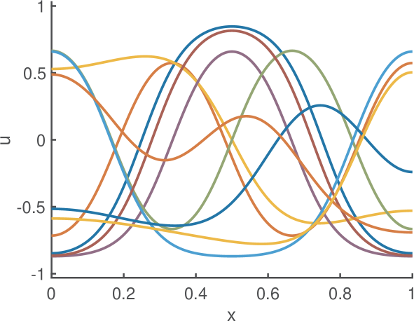
Figure 1. Ten sample validated one-dimensional equilibrium solutions. For all solutions we choose $\lambda=150$ and $\sigma=6$. Three of the solutions have total mass $\mu=0$, three are for mass $\mu=0.1$, three for $\mu=0.3$, and finally one for $\mu=0.5$.

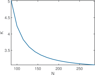
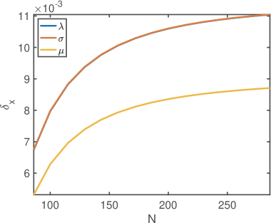
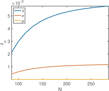
Figure 2. There is a tradeoff between high-dimensional calculations and optimal results. The top left figure shows how the bound of $K$ varies with the dimension of the truncated approximation matrix used to calculate $K_{N}$. These calculations are for dimension one, but a similar effect occurs in higher dimensions as well. The top right figure shows the corresponding estimate for $\delta_{x}$, and the bottom panel shows the estimate for $\delta_{\alpha}$, where $\alpha$ is each of the three parameters. The size of the validated interval grows larger as the truncation dimension grows, but with diminishing returns on the computational investment.

$\mu$	$K$	$N$	$P$	$\delta_{\alpha}$	$\delta_{x}$
$0$	6.2575	89	$\lambda$	0.0016	0.0056
			$\sigma$	2.9259e-04	0.0056
			$\mu$	2.8705e-06	0.0044
$0.1$	6.4590	104	$\lambda$	0.0011	0.0050
			$\sigma$	2.5369e-04	0.0050
			$\mu$	2.5579e-06	0.0041
$0.5$	3.1030	74	$\lambda$	0.0052	0.0107
			$\sigma$	0.0011	0.0106
			$\mu$	1.2871e-05	0.0092

Table 2. A sample of the one-dimensional solution validation parameters for three typical solutions. In each case, we use $\sigma=6$ and $\lambda=150$. If we had chosen a larger value of $N$, we could significantly improve the results.

Under the hypotheses of Theorem 2.1, the constructive implicit function theorem, for each $\delta_{\alpha}$ and $\delta_{x}$ satisfying both parts of (4), we are guaranteed that the solution is uniquely contained in the corresponding $(\delta_{\alpha},\delta_{x})$-box, where $\alpha$ is the chosen of the three parameters. In fact, if we fix $\delta_{\alpha}$ small enough, then there are a range of values of $\delta_{x}$ bounded below by the quadratic second equation and above by the linear first equation. We can view the region bounded by the lower limit of $\delta_{x}$ as an accuracy region, within which the equilibrium is guaranteed to lie; and the region bounded by the upper limit of $\delta_{x}$ is a uniqueness region, which contains the accuracy region, within which the solution is guaranteed to be unique. If $\delta_{\alpha}$ is chosen to be the point for which the line and curve in (4) intersect, then this is the largest possible value of $\delta_{\alpha}$ for which the theorem holds, and the accuracy and uniqueness regions coincide. In our calculations we have validated using this maximal interval in parameter space, and we have done the calculation of the interval size for each of the three parameters.

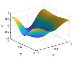
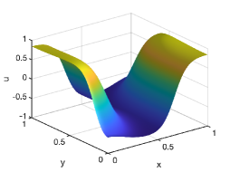
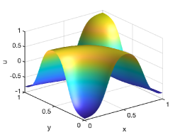
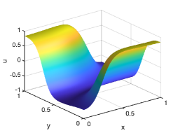
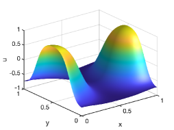
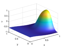
Figure 3. Six of the seventeen validated two-dimensional equilibrium solutions. For all seventeen solutions we use $\sigma=6$. Five of these solutions are for $\lambda=75$ and $\mu=0$ (top left). The rest of them use $\lambda=150$ and $\mu=0$ (top middle and top right), $\mu=0.1$ (bottom left), $\mu=0.3$ (bottom middle), and $\mu=0.5$ (bottom right).

$(\lambda,\mu)$	$K$	$N$	$P$	$\delta_{\alpha}$	$\delta_{x}$
$(75,0)$	21.1303	28	$\lambda$	1.6124e-04	0.0020
			$\sigma$	6.1338e-05	0.0020
			$\mu$	5.9914e-07	0.0016
$(150,0.1)$	30.1656	72	$\lambda$	1.1833e-05	4.7710e-04
			$\sigma$	5.1514e-06	4.7858e-04
			$\mu$	4.4558e-08	4.2316e-04

Table 3. A sample of the two-dimensional validation parameters for a couple of typical solutions. In all cases, we use $\sigma=6$. Again as in the previous table, we could improve results by choosing a larger value of $N$, but in this case since $N$ is only the linear dimension, the dimension of the calculation varies with $N^{2}$.

We have validated ten different equilibrium solutions in one dimension, shown in Figure 1. Some examples of the associated validation parameters are presented in Table 2. Ideally, we are able to validate the largest possible $(\delta_{\alpha},\delta_{x})$-box in which we can guarantee that the solution exists. However, there is a tradeoff between computational cost and optimal bounds. The most computationally costly part of our estimates is the calculation of $K_{N}$, the bound on the inverse of the linearization of the truncated system. As depicted in Figure 2, the bounds on $K$, and correspondingly on $\delta_{x}$ and $\delta_{\alpha}$, depend significantly on the value of $N$ that is chosen for the truncation dimension. Since our goal is to use these validations iteratively for path following, we will not be able to refine our calculations each time. Therefore as a rule of thumb for a starting point, we used the equation in Theorem 3.1 to guess that we would have a successful validation for $N\approx C\|q\|^{1/2}_{H^{2}}$, where $C$ is a fixed order one constant. In our calculations for the ten solutions, this results in a dimension that varies. For these calculations we chose $N$ values ranging between 50 and 200. The values of $M_{i}$ become progressively larger as you go from $\lambda$ to $\sigma$ to $\mu$. This means that the corresponding values of $\delta_{\alpha}$ are worse (i.e., smaller), respectively, often by one or two orders of magnitude. However, the values of $\delta_{x}$ for the three cases are of the same order. While we could increase $N$ to improve the estimates, Figure 2 shows that there are diminishing returns on computational investment, and eventually at some $N$, we could not have done much better even with a significantly larger value of $N$.

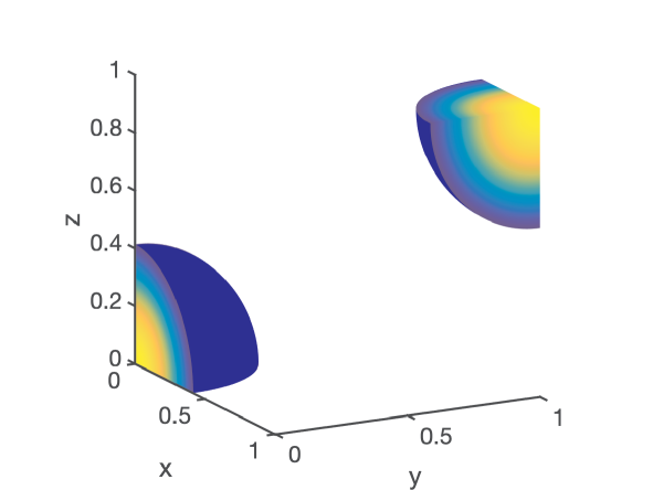
Figure 4. A three-dimensional validated solution for the parameter values $\lambda=75$, $\sigma=6$, and $\mu=0$.

$(\lambda,\sigma,\mu)$	$K$	$N$	$P$	$\delta_{\alpha}$	$\delta_{x}$
$(75,6,0)$	22.6527	22	$\lambda$	0.1143e-04	0.5917e-03
			$\sigma$	0.1707e-04	0.5955e-03
			$\mu$	0.0010e-04	0.4901e-03

Table 4. Validation parameters for a three-dimensional sample solution.

In two dimensions, we have validated seventeen different solutions for varying parameter values. A representative sample are given in Figure 3, with some sample validation parameters presented in Table 3. Again here, there is a tradeoff between computational speed and optimal results, but with all of the computations being significantly longer due to the increased dimension; if the function $u$ is encoded by a Fourier coefficient array of size $N\times N$, then the derivative matrix is of size $(N^{2}-1)^{2}$, where the $-1$ is due to the fact that we have removed the constant term. As in one dimension, the resulting $\delta_{\alpha}$ values vary significantly, but the $\delta_{x}$ values do not. Figure 4 and Table 4 show the details of a solution which is validated in three dimensions, with much the same observed behavior. Three-dimensional result validation requires a much larger computational effort, since if the function $u$ is given by a Fourier coefficient array of size $N\times N\times N$, then the derivative matrices with inverse being approximated are of size $(N^{3}-1)^{2}$.

6. Conclusions

As outlined in more detail in the introduction, in this paper we presented the theoretical foundations for validating branch segments of equilibrium solutions for the diblock copolymer model. Our approach is based on using the natural Sobolev norms which are used in the study of the underlying evolution equation, and they have been derived in all three relevant physical dimensions. As a side result, we obtained a method based on Neumann series to determine rigorous upper bounds on the inverse Fréchet derivative of the diblock copolymer operator which are of interest in their own right, as they are connected to the pseudo-spectrum of this non-self-adjoint operator, see [31]. Moreover, we have demonstrated briefly in the last section how these results can be used to obtain computer-assisted proofs for selected diblock copolymer equilibrium solutions.

While the present paper is a first step towards a complete path-following framework for the diblock copolymer model in dimensions up to three, there are still a number of issues that have to be addressed. On the theoretical side, one has to develop a pseudo-arclength continuation method with associated linking conditions which operates in an automatic fashion. This can be done by using the constructive implicit function theorem as a tool, similar to the applications to slanted box continuation and limit point resolution which were presented in [30, Sections 2.2 and 2.3]. In addition, the bottleneck in the current validation step is the estimation of the norm bound for the inverse. Especially in two, and even more so in three dimensions, one has to implement path-following in such a way that the estimate does not have to be validated at every step. This can be accomplished via perturbation arguments, and further speedups are possible by using the sparseness of the involved matrices. However, all of these issues are nontrivial and lie beyond the scope of the current paper — they will therefore be presented elsewhere.

References

- [1] R. A. Adams and J. J. F. Fournier. Sobolev Spaces. Elsevier/Academic Press, Amsterdam, second edition, 2003.
- [2] G. Arioli and H. Koch. Computer-assisted methods for the study of stationary solutions in dissipative systems, applied to the Kuramoto-Sivashinski equation. Archive for Rational Mechanics and Analysis, 197(3):1033–1051, 2010.
- [3] S. Cai and Y. Watanabe. A computer-assisted method for the diblock copolymer model. Zeitschrift für Angewandte Mathematik und Mechanik, 99(7):e201800125, 14, 2019.
- [4] L. Chierchia. KAM lectures. In Dynamical systems. Part I, pages 1–55. Scuola Normale Superiore, Pisa, Italy, 2003.
- [5] R. Choksi, M. Maras, and J. F. Williams. 2D phase diagram for minimizers of a Cahn-Hilliard functional with long-range interactions. SIAM Journal on Applied Dynamical Systems, 10(4):1344–1362, 2011.
- [6] R. Choksi, M. A. Peletier, and J. F. Williams. On the phase diagram for microphase separation of diblock copolymers: An approach via a nonlocal Cahn-Hilliard functional. SIAM Journal on Applied Mathematics, 69(6):1712–1738, 2009.
- [7] R. Choksi and X. Ren. On the derivation of a density functional theory for microphase separation of diblock copolymers. Journal of Statistical Physics, 113:151–76, 2003.
- [8] R. Choksi and X. Ren. Diblock copolymer/homopolymer blends: derivation of a density functional theory. Physica D, 203(1-2):100–119, 2005.
- [9] J. Cyranka and T. Wanner. Computer-assisted proof of heteroclinic connections in the one-dimensional Ohta-Kawasaki model. SIAM Journal on Applied Dynamical Systems, 17(1):694–731, 2018.
- [10] S. Day, J.-P. Lessard, and K. Mischaikow. Validated continuation for equilibria of PDEs. SIAM Journal on Numerical Analysis, 45(4):1398–1424, 2007.
- [11] J. P. Desi, H. Edrees, J. Price, E. Sander, and T. Wanner. The dynamics of nucleation in stochastic Cahn-Morral systems. SIAM Journal on Applied Dynamical Systems, 10(2):707–743, 2011.
- [12] A. Dhooge, W. Govaerts, and Y. A. Kuznetsov. MATCONT: a MATLAB package for numerical bifurcation analysis of ODEs. Association for Computing Machinery. Transactions on Mathematical Software, 29(2):141–164, 2003.
- [13] E. Doedel. AUTO: a program for the automatic bifurcation analysis of autonomous systems. In Proceedings of the Tenth Manitoba Conference on Numerical Mathematics and Computing, Vol. I (Winnipeg, Man., 1980), volume 30, pages 265–284, 1981.
- [14] M. Gameiro, J.-P. Lessard, and K. Mischaikow. Validated continuation over large parameter ranges for equilibria of PDEs. Mathematics and Computers in Simulation, 79(4):1368–1382, 2008.
- [15] Z. G. Huseynov and A. M. Shykhammedov. On bases of sines and cosines in Sobolev spaces. Applied Mathematics Letters, 25(3):275–278, 2012.
- [16] I. Johnson, E. Sander, and T. Wanner. Branch interactions and long-term dynamics for the diblock copolymer model in one dimension. Discrete and Continuous Dynamical Systems. Series A, 33(8):3671–3705, 2013.
- [17] T. Kinoshita, Y. Watanabe, and M. T. Nakao. An alternative approach to norm bound computation for inverses of linear operators in Hilbert spaces. Journal of Differential Equations, 266(9):5431–5447, 2019.
- [18] J.-P. Lessard, E. Sander, and T. Wanner. Rigorous continuation of bifurcation points in the diblock copolymer equation. Journal of Computational Dynamics, 4(1–2):71–118, 2017.
- [19] S. Maier-Paape, U. Miller, K. Mischaikow, and T. Wanner. Rigorous numerics for the Cahn-Hilliard equation on the unit square. Revista Matematica Complutense, 21(2):351–426, 2008.
- [20] S. Maier-Paape, K. Mischaikow, and T. Wanner. Structure of the attractor of the Cahn-Hilliard equation on a square. International Journal of Bifurcation and Chaos, 17(4):1221–1263, 2007.
- [21] S. Maier-Paape and T. Wanner. Spinodal decomposition for the Cahn-Hilliard equation in higher dimensions: Nonlinear dynamics. Archive for Rational Mechanics and Analysis, 151(3):187–219, 2000.
- [22] T. R. Muradov and V. F. Salmanov. On the basis property of trigonometric systems with linear phase in a weighted Sobolev space. Rossiĭskaya Akademiya Nauk. Doklady Akademii Nauk, 458(5):523–525, 2014.
- [23] M. T. Nakao, M. Plum, and Y. Watanabe. Numerical Verification Methods and Computer-Assisted Proofs for Partial Differential Equations. Springer-Verlag, Berlin, 2019.
- [24] T. Ohta and K. Kawasaki. Equilibrium morphology of block copolymer melts. Macromolecules, 19:2621–2632, 1986.
- [25] M. Plum. Existence and enclosure results for continua of solutions of parameter-dependent nonlinear boundary value problems. Journal of Computational and Applied Mathematics, 60(1-2):187–200, 1995.
- [26] M. Plum. Enclosures for two-point boundary value problems near bifurcation points. In Scientific computing and validated numerics (Wuppertal, 1995), volume 90 of Mathematical Research, pages 265–279. Akademie Verlag, Berlin, 1996.
- [27] M. Plum. Computer-assisted proofs for semilinear elliptic boundary value problems. Japan Journal of Industrial and Applied Mathematics, 26(2-3):419–442, 2009.
- [28] S. M. Rump. INTLAB - INTerval LABoratory. In T. Csendes, editor, Developments in Reliable Computing, pages 77–104. Kluwer Academic Publishers, Dordrecht, 1999. http://www.ti3.tuhh.de/rump/.
- [29] S. M. Rump. Verification methods: rigorous results using floating-point arithmetic. Acta Numerica, 19:287–449, 2010.
- [30] E. Sander and T. Wanner. Validated saddle-node bifurcations and applications to lattice dynamical systems. SIAM Journal on Applied Dynamical Systems, 15(3):1690–1733, 2016.
- [31] L. N. Trefethen and M. Embree. Spectra and Pseudospectra. Princeton University Press, Princeton, NJ, 2005.
- [32] J. B. van den Berg and J. F. Williams. Validation of the bifurcation diagram in the 2D Ohta-Kawasaki problem. Nonlinearity, 30(4):1584–1638, 2017.
- [33] J. B. van den Berg and J. F. Williams. Optimal periodic structures with general space group symmetries in the Ohta-Kawasaki problem. arXiv:1912.00059, 2019.
- [34] J. B. van den Berg and J. F. Williams. Rigorously computing symmetric stationary states of the Ohta-Kawasaki problem in three dimensions. SIAM Journal on Mathematical Analysis, 51(1):131–158, 2019.
- [35] T. Wanner. Topological analysis of the diblock copolymer equation. In Y. Nishiura and M. Kotani, editors, Mathematical Challenges in a New Phase of Materials Science, volume 166 of Springer Proceedings in Mathematics & Statistics, pages 27–51. Springer-Verlag, 2016.
- [36] T. Wanner. Computer-assisted equilibrium validation for the diblock copolymer model. Discrete and Continuous Dynamical Systems, Series A, 37(2):1075–1107, 2017.
- [37] T. Wanner. Computer-assisted bifurcation diagram validation and applications in materials science. Proceedings of Symposia in Applied Mathematics, 74:123–174, 2018.
- [38] T. Wanner. Validated bounds on embedding constants for Sobolev space Banach algebras. Mathematical Methods in the Applied Sciences, 41(18):9361–9376, 2018.
- [39] Y. Watanabe, T. Kinoshita, and M. T. Nakao. An improved method for verifying the existence and bounds of the inverse of second-order linear elliptic operators mapping to dual space. Japan Journal of Industrial and Applied Mathematics, 36(2):407–420, 2019.
- [40] Y. Watanabe, K. Nagatou, M. Plum, and M. T. Nakao. Norm bound computation for inverses of linear operators in Hilbert spaces. Journal of Differential Equations, 260(7):6363–6374, 2016.
- [41] N. Yamamoto. A numerical verification method for solutions of boundary value problems with local uniqueness by Banach’s fixed-point theorem. SIAM Journal on Numerical Analysis, 35(5):2004–2013, 1998.
- [42] N. Yamamoto, M. T. Nakao, and Y. Watanabe. A theorem for numerical verification on local uniqueness of solutions to fixed-point equations. Numerical Functional Analysis and Optimization, 32(11):1190–1204, 2011.