Error analysis of Nitsche’s and discontinuous Galerkin methods of a reduced Landau-de Gennes problem

Abstract

We study a system of semi-linear elliptic partial differential equations with a lower order cubic nonlinear term, and inhomogeneous Dirichlet boundary conditions, relevant for two-dimensional bistable liquid crystal devices, within a reduced Landau-de Gennes framework. The main results are (i) a priori error estimates for the energy norm, within the Nitsche’s and discontinuous Galerkin frameworks under milder regularity assumptions on the exact solution and (ii) a reliable and efficient a posteriori analysis for a sufficiently large penalization parameter and a sufficiently fine triangulation in both cases. Numerical examples that validate the theoretical results, are presented separately.

Keywords: non-linear elliptic pde, non-homogeneous Dirichlet boundary data, lower regularity, Nitsche’s method, dG method, a priori and a posteriori error estimates, adaptive finite element methods

1 Introduction

This paper focuses on the numerical analysis of a system of two second order semi-linear elliptic partial differential equations, with a lower order cubic non-linearity, defined on bounded two-dimensional domains with Lipschitz boundaries and inhomogeneous boundary conditions. Such systems arise naturally in different contexts for two-dimensional systems, our primary motivation being two-dimensional liquid crystal systems [11]. Liquid crystals are intermediate phases of matter between the conventional solid and liquid states of matter with versatile properties of both phases. Nematic liquid crystals are amongst the most commonly used liquid crystals, for which the constituent rod-like molecules translate freely but exhibit locally preferred directions of orientational ordering, and these locally distinguished directions are referred to as nematic directors [11]. Consequently, nematics are directional or anisotropic materials with direction-dependent physical properties. The Landau-de Gennes (LdG) theory is perhaps the most celebrated continuum theory for nematic liquid crystals, that describes the nematic state by the LdG order parameter - Q-tensor order parameter: a symmetric traceless $3\times 3$ matrix that contains information about the nematic directors and the degree of orientational ordering, within the matrix eigenvectors and eigenvalues, respectively [26]. Reduced two-dimensional LdG approaches have been rigorously derived for two-dimensional domains [13, 35], for certain model situations. In the reduced case, the order parameter is a symmetric, traceless $2\times 2$ matrix, with simply two independent components, $u$ and $v$. More precisely, if $\mathbf{n}=\left(\cos\theta,\sin\theta\right)$ is the nematic director in the plane, where $\theta\in\left[0,2\pi\right)$ and $s$ is a scalar order parameter that measures the degree of orientational order, then $u=s\cos 2\theta$ and v =$s\sin 2\theta$. Define the two-dimensional vector, $\Psi:=\left(u,v\right)$ on an open, bounded domain, $\Omega\subset\mathbb{R}^{2}$, with a polygonal boundary, $\partial\Omega$. Then for Dirichlet boundary conditions and in the absence of external fields, the dimensionless reduced LdG free energy [22] is

$$\mathcal{E}(\Psi_{\epsilon})=\int_{\Omega}(|\nabla\Psi_{\epsilon}|^{2}+\epsilon^{-2}(|\Psi_{\epsilon}|^{2}-1)^{2})\,{\rm dx},$$ (1.1)

where $\Psi_{\epsilon}=\mathbf{g}$ on $\partial\Omega$, and $\epsilon$ is a material-dependent parameter that depends on the elastic constant, domain size and temperature. Informally speaking, the limit $\epsilon\to 0$ corresponds to macroscopic domains with size much greater than material-dependent characteristic nematic correlation lengths [25]. The experimentally observable and physically relevant states are local or global minimizers of the reduced energy, which are weak solutions, $\Psi_{\epsilon}\in\mathbf{H}^{1}(\Omega):=H^{1}(\Omega)\times H^{1}(\Omega)$, of the corresponding Euler-Lagrange equations:

$$-\Delta\Psi_{\epsilon}=2\epsilon^{-2}(1-|\Psi_{\epsilon}|^{2})\Psi_{\epsilon}\text{ in }\Omega\,\,\text{ and }\,\,\Psi_{\epsilon}=\mathbf{g}\text{ on }\partial\Omega.$$ (1.2)

In what follows, we work with fixed but small values of $\epsilon$, which describe large domains [16]. The non-linear system (1.2) is a Poisson-type equation for a two-dimensional vector with a non-linear (cubic) lower order term. In fact, these equations are the celebrated Ginzburg-Landau partial differential equations with a rescaled $\epsilon$, which have been extensively studied in [3, 28]. In this paper, we apply Nitsche’s finite-element approximation method to this system (1.2) and our main contribution is to relax regularity assumptions on $\Psi_{\epsilon}$, as will be explained below. The Nitsche’s method is well-studied in the literature; see [15], [17], [23], [27] for applications of Nitsche’s method to Poisson’s equation with different boundary conditions, a priori and a posteriori error analysis for such problems and applications of medius analysis. Further results for the a posteriori analysis of the Poisson problem are also given in [5] with a saturation assumption, that can be stated as the approximate solution of the problem in a finer mesh constitutes a better approximation to the exact solution than the approximate solution on a coarser mesh, in the energy norm. In [2] and [20], the authors derive a posteriori error bounds for the finite-element analysis of the Poisson’s equation with $C^{0}$- Dirichlet boundary conditions, without the saturation assumption. Further, a priori and a posteriori error analysis of dGFEM (Discontinuous Galerkin Finite Element Methods) for the von Kármán equations are studied in [8]. The references are not exhaustive and the techniques in these papers are adapted to deal with the novel aspects of our problem, as will be outlined below.

The specific model (1.2) has been applied with success to the planar bistable nematic device reported in [33], where the authors study nematic liquid crystals-filled shallow square wells, with experimentally imposed tangent boundary conditions. They report the existence of six distinct stable solutions: two diagonal and four rotated solutions. The nematic director is aligned along the square diagonals in the diagonal solutions, and rotates by $\pi$ radians for the rotated solutions. In [22], the authors study the numerical convergence of the diagonal and rotated solutions, in a conforming finite-element set-up, as a function of $\epsilon$. In [24], the authors carry out a rigorous a priori error analysis for the dGFEM approximation of $\mathbf{H}^{2}$-regular solutions of (1.2) in convex polygonal domains. Optimal linear (resp. quadratic) order of convergence in energy (resp. $\mathbf{L}^{2}$) norm for solutions, $\Psi_{\epsilon}\in\mathbf{H}^{2}(\Omega)$, accompanied by an analysis of the $h-\epsilon$ dependency, where $h$ is the mesh size or the discretization parameter, along with some numerical experiments are discussed. However, there are no a posteriori error estimates in [24]. This paper builds on the results in [24] with several non-trivial generalisations and extensions. Define the admissible space $\boldsymbol{\mathcal{{X}}}=\left\{\mathbf{w}\in\mathbf{H}^{1}(\Omega):\mathbf{w}=\mathbf{g}\,\,\text{on}\,\,\partial\Omega\right\}$ and we restrict attention to solutions $\Psi_{\epsilon}\!\in\!\boldsymbol{\mathcal{{X}}}\cap\mathbf{H}^{1+\alpha}(\Omega)$ for $0<\alpha\leq 1$, where $\alpha$ is the index of elliptic regularity in this manuscript. The main contributions of this article are summarised below:

• an a priori finite element error analysis for (1.2), using the Nitsche’s method to incorporate the non-homogeneous boundary conditions, along with a proof of $h^{\alpha}$ (resp. $h^{2\alpha}$)-convergence of the energy (resp. $\mathbf{L}^{2}$) norm where $h$ is the discretization parameter;

• a reliable and efficient residual type a posteriori error estimate for (1.2) with the assumption that the boundary function, $\mathbf{g}\in\mathbf{H}^{\frac{1}{2}}(\partial\Omega)$ belongs to $\mathbf{C}^{0}(\overline{\partial\Omega})$;

• a priori and a posteriori error estimates for dGFEM under the mild regularity assumption, $\Psi_{\epsilon}\in\boldsymbol{\mathcal{{X}}}\cap\mathbf{H}^{1+\alpha}(\Omega)$ for $0<\alpha\leq 1$;

• numerical experiments for uniform as well as adaptive refinement that validate the theoretical estimates above.

There are new technical challenges in this manuscript, compared to [24]. The analysis in [24] is restricted to solutions in $\mathbf{H}^{2}(\Omega)$, or equivalently $\alpha=1$. The first challenge with a less regular solution, $\Psi_{\epsilon}$ as above, is to handle the normal derivatives $\nabla\Psi_{\epsilon}\nu\notin\mathbf{L}^{2}(E)$ across the element boundaries. In this paper, the medius analysis [15] that combines ideas of both a posteriori and a priori analysis is employed to overcome this. New local efficiency results are proved to establish the stability of a perturbed bilinear form. For the a posteriori analysis, a lifting operator $\Psi_{\mathbf{g}}$ is used such that $\Psi_{\mathbf{g}}=\mathbf{g}$ on $\partial\Omega$, and this technique requires the additional continuity constraints on $\mathbf{g}$. These continuity constraints might be relaxed by using saturation techniques, and will be pursued in future work. The generalisations to dGFEM with $\alpha<1$, involve additional jump and average terms, due to the lack of inter-element continuity in the dGFEM discrete space. For $\alpha=1$, there are $\epsilon$-independent estimates for the $H^{2}$-norm of solutions, $\Psi_{\epsilon}$ (see[4]) which allows for a $h-\epsilon$ dependency study in [24]; this is not easily possible for $\alpha<1$ and hence, the value of $\epsilon$ is fixed in this manuscript, unlike the study in [24].

The reduced regularity assumption for the exact solution is relevant for non-convex polygons, domains with re-entrant corners or slit edges, with $\alpha<1$ [14]. Further, a posteriori error estimators provide a systematic way of controlling errors for adaptive mesh refinements [1, 34], as is illustrated by means of several numerical experiments in Section 6. The numerical estimates confirm the a priori and a posteriori estimates and establishes the advantages of adaptive mesh refinements in terms of computational cost and rates of convergence, captured by informative convergence plots for the estimators in Section 6.

The standard notation for Sobolev spaces $H^{s}(\Omega)$ $(\text{resp.}\,W^{s,p}(\Omega))$ with $s,p$ positive real numbers, equipped with the usual norm ${|\kern-1.07639pt|\cdot|\kern-1.07639pt|}_{s}$ $(\text{resp. }{|\kern-1.07639pt|\cdot|\kern-1.07639pt|}_{s,p})$ is used throughout the paper and the space $\mathbf{H}^{s}(\Omega)$ (resp. $\mathbf{L}^{p}(\Omega)$) is defined to be the product space $H^{s}(\Omega)\times H^{s}(\Omega)$ $(\text{resp. }L^{p}(\Omega)\times L^{p}(\Omega))$ equipped with the corresponding norm ${|\kern-1.07639pt|\kern-1.07639pt|\cdot|\kern-1.07639pt|\kern-1.07639pt|}_{s}$ ($\text{resp. }{|\kern-1.07639pt|\kern-1.07639pt|\cdot|\kern-1.07639pt|\kern-1.07639pt|}_{s,p}$) defined by ${|\kern-1.07639pt|\kern-1.07639pt|\Phi|\kern-1.07639pt|\kern-1.07639pt|}_{s}\!=({|\kern-1.07639pt|\varphi_{1}|\kern-1.07639pt|}_{s}^{2}+{|\kern-1.07639pt|\varphi_{2}|\kern-1.07639pt|}_{s}^{2})^{\frac{1}{2}}$ for all $\Phi\!=\!(\varphi_{1},\varphi_{2})\in\!\mathbf{H}^{s}(\Omega)$ $(\text{resp. }{|\kern-1.07639pt|\kern-1.07639pt|\Phi|\kern-1.07639pt|\kern-1.07639pt|}_{s,p}\!\!=({|\kern-1.07639pt|\varphi_{1}|\kern-1.07639pt|}_{s,p}^{2}+{|\kern-1.07639pt|\varphi_{2}|\kern-1.07639pt|}_{s,p}^{2})^{\frac{1}{2}}$ for all $\Phi\!=\!(\varphi_{1},\varphi_{2})\!\in\!\mathbf{W}^{s,p}(\Omega)).$ The norm on $\mathbf{L}^{2}(\Omega)$ space is simply ${|\kern-1.07639pt|\kern-1.07639pt|\Phi|\kern-1.07639pt|\kern-1.07639pt|}_{0}\!=({|\kern-1.07639pt|\varphi_{1}|\kern-1.07639pt|}_{0}^{2}+{|\kern-1.07639pt|\varphi_{2}|\kern-1.07639pt|}_{0}^{2})^{\frac{1}{2}}$ for all $\Phi\!=\!(\varphi_{1},\varphi_{2})\in\!\mathbf{L}^{2}(\Omega).$ Set $V:=H_{0}^{1}(\Omega)=\big{\{}\varphi\in L^{2}(\Omega):\frac{\partial\varphi}{\partial x},\frac{\partial\varphi}{\partial y}\in L^{2}(\Omega),$ $\varphi|_{\partial{\Omega}}=0\big{\}}$ and $\mathbf{V}\!=\,\!\mathbf{H}_{0}^{1}(\Omega)=H_{0}^{1}(\Omega)\times H_{0}^{1}(\Omega)$. Throughout the manuscript, $C_{s}$ denotes a generic constant.

The paper is organized as follows. In the next section, the weak formulation and the Nitsche’s method are introduced. Section 2.3 is devoted to the main results for both a priori and a posteriori error analysis for Nitsche’s method. Section 3 contains some auxiliary results followed by the rigorous a priori error estimates for Nitsche’s method. In Section 4, a reliable and efficient a posteriori error analysis for Nitsche’s method is presented. Section 5 focuses on the the generalisations to dGFEM and is followed by numerical experiments that confirm the theoretical findings in Section 6. Section 7 concludes with some brief perspectives. The proofs of the local efficiency results are given in the Appendix.

2 Preliminaries and main results

The weak formulation of the non-linear system (1.2), the Nitsche’s method and the main results in the Nitsche framework are given in this section.

2.1 Weak formulation

The weak formulation of (1.2) seeks $\Psi_{\epsilon}\in\boldsymbol{\mathcal{{X}}}$ such that for all $\Phi\in\mathbf{V}$,

$$N(\Psi_{\epsilon};\Phi):=A(\Psi_{\epsilon},\Phi)+B(\Psi_{\epsilon},\Psi_{\epsilon},\Psi_{\epsilon},\Phi)+C(\Psi_{\epsilon},\Phi)=0.\,\,\,\,$$ (2.1)

Here for all $\Xi=(\xi_{1},\xi_{2}),\boldsymbol{\eta}=(\eta_{1},\eta_{2}),\Theta=(\theta_{1},\theta_{2}),\Phi=(\varphi_{1},\varphi_{2})\in\mathbf{X}:=\mathbf{H}^{1}(\Omega),$

$$A(\Theta,\Phi):=a(\theta_{1},\varphi_{1})+a(\theta_{2},\varphi_{2}),\,\,C(\Theta,\varphi):=c(\theta_{1},\varphi_{1})+c(\theta_{2},\varphi_{2}),$$

$$B(\Xi,\boldsymbol{\eta},\Theta,\Phi):=\frac{2}{3\epsilon^{2}}\int_{\Omega}\left((\Xi\cdot\boldsymbol{\eta})(\Theta\cdot\Phi)+2(\Xi\cdot\Theta)(\boldsymbol{\eta}\cdot\Phi)\right)\,{\rm dx}=\frac{1}{3}(3b(\xi_{1},\eta_{1},\theta_{1},\varphi_{1})+3b(\xi_{2},\eta_{2},\theta_{2},\varphi_{2})$$

$$\qquad\qquad\qquad\qquad+2b(\xi_{2},\eta_{1},\theta_{2},\varphi_{1})+2b(\xi_{1},\eta_{2},\theta_{1},\varphi_{2})+b(\xi_{2},\eta_{2},\theta_{1},\varphi_{1})+b(\xi_{1},\eta_{1},\theta_{2},\varphi_{2})),$$

$$\text{and for }\xi,\eta,\theta,\varphi\in H^{1}(\Omega),\>a(\theta,\varphi):=\int_{\Omega}\nabla\theta\cdot\nabla\varphi\,{\rm dx},\>b(\xi,\eta,\theta,\varphi):=2\epsilon^{-2}\int_{\Omega}\xi\eta\theta\varphi\,{\rm dx}$$

$$\text{ and }c(\theta,\varphi):=-2\epsilon^{-2}\int_{\Omega}\theta\varphi\,{\rm dx}.$$

See [22, 24] for a proof of existence of minimizers of the Landau-de Gennes energy functional (1.1) that are solutions to (2.1). The analysis of this article is applicable to the cases where the exact solution $\Psi_{\epsilon}$ of (2.1) belongs to $\boldsymbol{\mathcal{{X}}}\cap\mathbf{H}^{1+\alpha}(\Omega),0<\alpha<1,$ for example in non-convex polygons. When $\Omega$ is a convex polygon, $\alpha=1$; that is, the solution of (2.1) belongs to $\boldsymbol{\mathcal{{X}}}\cap\mathbf{H}^{2}(\Omega)$. The regular solutions (also referred to as non-singular solutions in literature; see [8] and the references therein) $\Psi_{\epsilon}$ of (1.2) for a fixed $\epsilon$ are approximated. This implies that the linearized operator $\langle DN(\Psi_{\epsilon})\cdot,\cdot\rangle$ is invertible in the Banach space and the following inf-sup conditions [12] hold:

$$0<\beta:=\inf_{\begin{subarray}{c}\Theta\in\mathbf{V}\\ {|\kern-0.75346pt|\kern-0.75346pt|\Theta|\kern-0.75346pt|\kern-0.75346pt|}_{1}=1\end{subarray}}\sup_{\begin{subarray}{c}\Phi\in\mathbf{V}\\ {|\kern-0.75346pt|\kern-0.75346pt|\Phi|\kern-0.75346pt|\kern-0.75346pt|}_{1}=1\end{subarray}}\langle DN(\Psi_{\epsilon})\Theta,\Phi\rangle,\text{ and }0<\beta=\inf_{\begin{subarray}{c}\Phi\in\mathbf{V}\\ {|\kern-0.75346pt|\kern-0.75346pt|\Phi|\kern-0.75346pt|\kern-0.75346pt|}_{1}=1\end{subarray}}\sup_{\begin{subarray}{c}\Theta\in\mathbf{V}\\ {|\kern-0.75346pt|\kern-0.75346pt|\Theta|\kern-0.75346pt|\kern-0.75346pt|}_{1}=1\end{subarray}}\langle DN(\Psi_{\epsilon})\Theta,\Phi\rangle,$$ (2.2)

where $\langle DN(\Psi_{\epsilon})\Theta,\Phi\rangle:=A(\Theta,\Phi)+3B(\Psi_{\epsilon},\Psi_{\epsilon},\Theta,\Phi)+C(\Theta,\Phi)$ and the inf-sup constant $\beta$ depends on $\epsilon$. Here and throughout the paper, $\langle\cdot,\cdot\rangle$ denotes the duality pairing between $\mathbf{V}^{*}$ and $\mathbf{V}$. The parameter $\epsilon$ in $\Psi_{\epsilon}$ is suppressed for notational brevity and is chosen fixed in the sequel.

2.2 Nitsche’s method

Consider a shape-regular triangulation $\mathcal{T}$ of $\Omega$ into triangles [10]. Define the mesh discretization parameter $h=\max_{T\in\mathcal{T}}h_{T},$ where $h_{T}=diam(T)$. Denote $\mathcal{E}_{h}^{i}$( resp. $\mathcal{E}_{h}^{\partial}$) to be the interior (resp. boundary) edges of $\mathcal{T}$ and let $\mathcal{E}:=\mathcal{E}_{h}^{i}\cup\mathcal{E}_{h}^{\partial}$. The length of an edge $E$ is denoted by $h_{E}.$ Define the finite element subspace of $\mathbf{X}$ by $\mathbf{X}_{h}:=X_{h}\times X_{h}$ with $X_{h}:=\{v\in H^{1}(\Omega)|\,\,v|_{T}\in P_{1}(T)\text{ for all }T\in\mathcal{T}\}$ and let the discrete norm be defined by $\displaystyle{|\kern-1.07639pt|v|\kern-1.07639pt|}^{2}_{h}:=\int_{\Omega}|\nabla v|^{2}\,{\rm dx}+\sum_{E\in\mathcal{E}_{h}^{\partial}}\frac{\sigma}{h_{E}}\int_{E}v^{2}\,{\rm ds}\text{ for all }v\in X_{h}.$ Here $\sigma>0$ is the penalty parameter and $P_{1}(T)$ denotes affine polynomials defined on $T$. The space $\mathbf{X}_{h}$ is equipped with the product norm ${|\kern-1.07639pt|\kern-1.07639pt|\Phi_{h}|\kern-1.07639pt|\kern-1.07639pt|}_{h}:=\left({|\kern-1.07639pt|\varphi_{1}|\kern-1.07639pt|}_{h}^{2}+{|\kern-1.07639pt|\varphi_{2}|\kern-1.07639pt|}_{h}^{2}\right)^{1/2}$ for all $\Phi_{h}=(\varphi_{1},\varphi_{2})\in\mathbf{X}_{h}$. Define ${|\kern-1.07639pt|\kern-1.07639pt|\Phi_{h}|\kern-1.07639pt|\kern-1.07639pt|}_{0,E}^{2}:={|\kern-1.07639pt|\varphi_{1}|\kern-1.07639pt|}_{0,E}^{2}+{|\kern-1.07639pt|\varphi_{2}|\kern-1.07639pt|}_{0,E}^{2}$ and ${|\kern-1.07639pt|\kern-1.07639pt|\Phi_{h}|\kern-1.07639pt|\kern-1.07639pt|}_{0,T}^{2}:={|\kern-1.07639pt|\varphi_{1}|\kern-1.07639pt|}_{0,T}^{2}+{|\kern-1.07639pt|\varphi_{2}|\kern-1.07639pt|}_{0,T}^{2}$ for $\Phi_{h}\in\mathbf{X}_{h}$ such that for $v\in X_{h},$ ${|\kern-1.07639pt|v|\kern-1.07639pt|}_{0,E}^{2}:=\int_{E}v^{2}\,{\rm ds}$ and ${|\kern-1.07639pt|v|\kern-1.07639pt|}_{0,T}^{2}:=\int_{T}v^{2}\,{\rm dx}$, respectively. Define $H^{1}(\mathcal{T}):=\{v\in L^{2}(\Omega)|\,v\in H^{1}(T)\text{ for all }T\in\mathcal{T}\}$ and $\mathbf{H}^{1}(\mathcal{T}):=H^{1}(\mathcal{T})\times H^{1}(\mathcal{T}).$ For an interior edge $E$ shared by the triangles $T^{+}$ and $T^{-}$, define the jump and average of $\varphi\in H^{1}(\mathcal{T})$ across $E$ as $[\varphi]_{E}:=\varphi|_{T^{+}}-\varphi|_{T^{-}}$ and $\{\varphi\}_{E}:=\frac{1}{2}(\varphi|_{T^{+}}+\varphi|_{T^{-}})$, respectively, and for an boundary edge $E$ of the triangle $T$, $[\varphi]_{E}:=\varphi|_{T}$ and $\{\varphi\}_{E}:=\varphi|_{T}$, respectively. For a vector function, jump and average are defined component-wise. For $\theta,\varphi\in H^{1}(\Omega)$, $\mathbf{g}=(g_{1},g_{2})$ and the penalty parameter $\sigma>0$, let

$$a_{h}(\theta,\varphi):=\int_{\Omega}\nabla\theta\cdot\nabla\varphi\,{\rm dx}-\langle\frac{\partial\theta}{\partial\nu},\varphi\rangle_{\partial\Omega}-\langle\theta,\frac{\partial\varphi}{\partial\nu}\rangle_{\partial\Omega}+\sum_{E\in\mathcal{E}_{h}^{\partial}}\frac{\sigma}{h_{E}}\langle\theta,\varphi\rangle_{E},$$

$$\text{ and }\,\,l^{i}_{h}(\varphi):=-\langle g_{i},\frac{\partial\varphi}{\partial\nu}\rangle_{\partial\Omega}+\sum_{E\in\mathcal{E}_{h}^{\partial}}\frac{\sigma}{h_{E}}\langle g_{i},\varphi\rangle_{E}\text{ for }1\leq i\leq 2,$$

where $\langle\cdot,\cdot\rangle_{\partial\Omega}$ denotes the duality pairing between ${H}^{-\frac{1}{2}}(\partial\Omega)$ and ${H}^{\frac{1}{2}}(\partial\Omega)$ and $\nu$ denotes the outward unit normal associated to $\partial\Omega$. In the sequel, $\langle\cdot,\cdot\rangle_{E}$ is the duality pairing between ${H}^{-\frac{1}{2}}(E)$ and ${H}^{\frac{1}{2}}(E)$ for $E\in\mathcal{E}.$ For $\Theta=(\theta_{1},\theta_{2}),\,\Phi=(\varphi_{1},\varphi_{2})\in\mathbf{X}$, let $A_{h}(\Theta,\Phi):=a_{h}(\theta_{1},\varphi_{1})+a_{h}(\theta_{2},\varphi_{2}),$ and $L_{h}(\Phi_{h})=l^{1}_{h}(\varphi_{1})+l^{2}_{h}(\varphi_{2})$.

The Nitsche’s method corresponding to (1.2) seeks $\Psi_{h}\!\in\!\mathbf{X}_{h}$, such that for all $\Phi_{h}\in\mathbf{X}_{h},$

$$N_{h}(\Psi_{h};\Phi_{h}):=A_{h}(\Psi_{h},\Phi_{h})+B(\Psi_{h},\Psi_{h},\Psi_{h},\Phi_{h})+C(\Psi_{h},\Phi_{h})-L_{h}(\Phi_{h})=0.$$ (2.3)

Remark 2.1.

The restrictions of the bilinear and quadrilinear forms $C(\cdot,\cdot),$ $B(\cdot,\cdot,\cdot,\cdot)$ to $T\in\mathcal{T}$ are denoted as $C_{T}(\cdot,\cdot),$ $B_{T}(\cdot,\cdot,\cdot,\cdot)$, respectively. Define the bilinear form $A_{T}(\Theta,\Phi):=\int_{T}\nabla\Theta\cdot\nabla\Phi\,{\rm dx}$ for all $\Theta,\Phi\in\mathbf{X}$. For $\Phi_{h}=(\varphi_{1},\varphi_{2})\in\mathbf{X}_{h}$, let $\nabla\Phi_{h}\nu_{E}:=(\frac{\partial\varphi_{1}}{\partial\nu_{E}},\frac{\partial\varphi_{2}}{\partial\nu_{E}})$ on an edge $E$ with outward unit normal $\nu_{E}$ to $E$.

2.3 Main results

The main results in this manuscript for Nitsche’s method are stated in this sub-section. Theorems 2.2 and 2.3 establish a priori error estimates in energy and $\mathbf{L}^{2}(\Omega)$ norms, and a posteriori error estimates for Nitsche’s method, respectively, when the exact solution $\Psi$ of (2.1) has the regularity $\boldsymbol{\mathcal{{X}}}\cap\mathbf{H}^{1+\alpha}(\Omega),\;0<\alpha\leq 1$. Throughout the sequel, $0<\alpha\leq 1$ denotes the index of elliptic regularity. The results are extended for dGFEM and are presented in Section 5.

Theorem 2.2.

(A priori error estimate) Let $\Psi$ be a regular solution of (2.1). For a sufficiently large penalty parameter $\sigma>0$, and a sufficiently small discretization parameter $h$, there exists a unique solution $\Psi_{h}$ to the discrete problem (2.3) that approximates $\Psi$ such that

$$(i)\,\,\,{|\kern-1.07639pt|\kern-1.07639pt|\Psi-\Psi_{h}|\kern-1.07639pt|\kern-1.07639pt|}_{h}\lesssim h^{\alpha},\quad(ii)\,\,\,{|\kern-1.07639pt|\kern-1.07639pt|\Psi-\Psi_{h}|\kern-1.07639pt|\kern-1.07639pt|}_{0}\lesssim h^{2\alpha},$$

where $0<\alpha\leq 1$ denotes the index of elliptic regularity. As per standard convention $a\lesssim b$ $\iff$ $a\leq Cb$ where the constant $C$ is independent of the discretization parameter $h$.

A reliable and efficient a posteriori error estimate for (2.3) is the second main result of the paper. For each element $T\!\in\!\mathcal{T}$ and edge $E\!\in\!\mathcal{E}$, define the volume and edge contributions to the estimators by

$$\vartheta_{T}^{2}:=h_{T}^{2}{|\kern-1.07639pt|\kern-1.07639pt|2\epsilon^{-2}(|\Psi_{h}|^{2}-1)\Psi_{h}|\kern-1.07639pt|\kern-1.07639pt|}^{2}_{0,T},\,\,\,(\vartheta_{E}^{i})^{2}:=h_{E}{|\kern-1.07639pt|\kern-1.07639pt|[\nabla\Psi_{h}\nu_{E}]_{E}|\kern-1.07639pt|\kern-1.07639pt|}_{0,E}^{2}\text{ for all }E\in\mathcal{E}_{h}^{i},$$ (2.4)

$$\text{and }(\vartheta_{E}^{\partial})^{2}:=\frac{1}{h_{E}}{|\kern-1.07639pt|\kern-1.07639pt|\Psi_{h}-\mathbf{g}|\kern-1.07639pt|\kern-1.07639pt|}_{0,E}^{2}\text{ for all }E\in\mathcal{E}_{h}^{\partial}.$$ (2.5)

Define the estimator $\displaystyle\vartheta^{2}:=\sum_{T\in\mathcal{T}}\vartheta_{T}^{2}+\sum_{E\in\mathcal{E}_{h}^{i}}(\vartheta_{E}^{i})^{2}+\sum_{E\in\mathcal{E}_{h}^{\partial}}(\vartheta_{E}^{\partial})^{2}.$

Theorem 2.3.

(A posteriori error estimate) Let $\Psi$ be a regular solution of (2.1) and $\Psi_{h}$ solve (2.3). For a sufficiently large penalty parameter $\sigma>0$, and a sufficiently small discretization parameter $h$, there exist $h$-independent positive constants $C_{\text{rel}}$ and $C_{\text{eff}}$ such that

$$C_{\text{eff}}\vartheta\leq{|\kern-1.07639pt|\kern-1.07639pt|\Psi-\Psi_{h}|\kern-1.07639pt|\kern-1.07639pt|}_{h}\leq C_{\text{rel}}\big{(}\vartheta+h.o.t\big{)},$$

where $h.o.t$ expresses one or several terms of higher order (as will be explained in Section 4).

3 A priori error estimate

This section is devoted to the proof of Theorem 2.2. Some auxiliary results are presented first. This is followed by a discrete inf-sup condition and the construction of a non-linear map for the application of Brouwer’s fixed point theorem. The energy and $\mathbf{L}^{2}$- norm estimates follow as a consequence of the fixed point and duality arguments.

3.1 Auxiliary results

Lemma 3.1.

(Poincaré type inequalities)[21] Let $\Omega$ be a bounded open subset of $\mathbb{R}^{2}$ with Lipschitz continuous boundary $\partial\Omega$.

1. For $\varphi\in H^{1}_{0}(\Omega)$, there exists a positive constant $\alpha_{0}=\alpha_{0}(\Omega)$ such that $\alpha_{0}{|\kern-1.07639pt|\varphi|\kern-1.07639pt|}_{0}\leq{|\kern-1.07639pt|\nabla\varphi|\kern-1.07639pt|}_{0}.$

2. For $\varphi\in H^{1}(\mathcal{T})$, there exists a constant $C_{P}>0$ independent of $h$ and $\varphi$ such that for $1\leq r<\infty$, ${|\kern-1.07639pt|\varphi|\kern-1.07639pt|}_{L^{r}(\Omega)}\leq C_{P}{|\kern-1.07639pt|\varphi|\kern-1.07639pt|}_{h}.$

Lemma 3.2 (Trace inequalities).

[12] $\displaystyle(i)\;\text{For }{\rm v}\!\in\!H^{1}(T),T\!\in\!\mathcal{T},{|\kern-1.07639pt|{\rm v}|\kern-1.07639pt|}_{0,\partial T}^{2}\lesssim(h_{T}^{-1}{|\kern-1.07639pt|{\rm v}|\kern-1.07639pt|}_{0,T}^{2}+{|\kern-1.07639pt|{\rm v}|\kern-1.07639pt|}_{0,T}{|\kern-1.07639pt|\nabla{\rm v}|\kern-1.07639pt|}_{0,T}).$ $\displaystyle(ii)\;\text{For all }\Phi_{h}\!\in\!\mathbf{X}_{h},\sum_{E\in\mathcal{E}_{h}^{\partial}}h_{E}{|\kern-1.07639pt|\kern-1.07639pt|\nabla\Phi_{h}\nu_{E}|\kern-1.07639pt|\kern-1.07639pt|}_{0,E}^{2}\lesssim{|\kern-1.07639pt|\kern-1.07639pt|\nabla\Phi_{h}|\kern-1.07639pt|\kern-1.07639pt|}_{0}^{2}.$

Lemma 3.3.

(Interpolation estimate)[10] For ${\rm v}\!\in\!H^{1+\alpha}(\Omega)\text{ with }\alpha\!\in\!(0,1]$, there exists ${\rm{I}}_{h}{\rm v}\!\in\!X_{h}$ such that

$${|\kern-1.07639pt|{\rm v}-{\rm{I}}_{h}{\rm v}|\kern-1.07639pt|}_{0}+h{|\kern-1.07639pt|{\rm v}-{\rm{I}}_{h}{\rm v}|\kern-1.07639pt|}_{1}\leq C_{I}h^{1+\alpha}|{\rm v}|_{H^{1+\alpha}(\Omega)},$$

where $C_{I}$ is a positive constant independent of $h$.

Remark 3.4.

Trace inequality stated in Lemma 3.2$(i)$ yields ${|\kern-1.07639pt|{\rm v}-{\rm{I}}_{h}{\rm v}|\kern-1.07639pt|}_{h}\leq C_{I}h^{\alpha}|{\rm v}|_{H^{1+\alpha}(\Omega)}$ for a positive constant $C_{I}$ independent of $h$.

Lemma 3.5.

(Extension operator) [6, 18, 23] Define the operator $\Pi_{h}:X_{h}\rightarrow V_{h}:=X_{h}\cap H^{1}_{0}(\Omega)$ using nodal values of freedom: $\displaystyle\Pi_{h}{\rm v}(n)=\begin{cases}0\quad\quad\text{ for a node }n\text{ on }\partial\Omega\\ {\rm v}(n)\quad\quad\text{ for a node }n\text{ on }\Omega\setminus\partial\Omega\end{cases}$. For all ${\rm v}\in X_{h}$, it holds that

$$\big{(}\sum_{T\in\mathcal{T}}h_{T}^{-2}{|\kern-1.07639pt|{\rm v}-\Pi_{h}{\rm v}|\kern-1.07639pt|}^{2}_{0,T}+\sum_{E\in\mathcal{E}_{h}^{i}}h_{E}^{-1}{|\kern-1.07639pt|{\rm v}-\Pi_{h}{\rm v}|\kern-1.07639pt|}^{2}_{0,E}\big{)}^{\frac{1}{2}}\leq C_{e_{1}}{|\kern-1.07639pt|{\rm v}|\kern-1.07639pt|}_{h},$$ (3.1)

$${|\kern-1.07639pt|{\rm v}-\Pi_{h}{\rm v}|\kern-1.07639pt|}_{h}\leq C_{e_{2}}(\sum_{E\in\mathcal{E}^{\partial}_{h}}h_{E}^{-1}\int_{E}{\rm v}^{2}{\rm ds})^{\frac{1}{2}}\leq C_{e_{2}}{|\kern-1.07639pt|{\rm v}|\kern-1.07639pt|}_{h},\quad{|\kern-1.07639pt|\Pi_{h}{\rm v}|\kern-1.07639pt|}_{h}\leq C_{e_{3}}{|\kern-1.07639pt|{\rm v}|\kern-1.07639pt|}_{h},$$ (3.2)

where the constants $C_{e_{1}}$, $C_{e_{2}}$ and $C_{e_{3}}$ are independent of $h$.

The next lemma states boundedness and coercivity results for $A(\cdot,\cdot)$ (resp. $A_{h}(\cdot,\cdot)$), boundedness results for $B(\cdot,\cdot,\cdot,\cdot)$ and $C(\cdot,\cdot)$. These results are a consequence of Hölder’s inequality, Lemma 3.1, and the Sobolev embedding results [10] $H^{1}(\Omega)\hookrightarrow L^{4}(\Omega)$ and $H^{1+\alpha}(\Omega)\hookrightarrow L^{\infty}(\Omega)$ for $\Omega\subset\mathbb{R}^{2}$ and $\alpha>0$. For detailed proofs, see [24].

Lemma 3.6.

(Properties of bilinear and quadrilinear forms)[24] The following properties hold.

1. For all $\Theta$, $\Phi\!\in\!\mathbf{V}$, $\displaystyle A(\Theta,\Phi)\leq{|\kern-1.07639pt|\kern-1.07639pt|\Theta|\kern-1.07639pt|\kern-1.07639pt|}_{1}{|\kern-1.07639pt|\kern-1.07639pt|\Phi|\kern-1.07639pt|\kern-1.07639pt|}_{1},\text{ and }A(\Theta,\Theta)\gtrsim{|\kern-1.07639pt|\kern-1.07639pt|\Theta|\kern-1.07639pt|\kern-1.07639pt|}_{1}^{2}.$

2. For the choice of a sufficiently large parameter $\sigma$, there exists a positive constant $C_{\rm ell}>0$ such that $\text{ for all }\Theta_{h},\Phi_{h}\in\mathbf{X}_{h}$, $\displaystyle A_{h}(\Theta_{h},\Phi_{h})\lesssim{|\kern-1.07639pt|\kern-1.07639pt|\Theta_{h}|\kern-1.07639pt|\kern-1.07639pt|}_{h}{|\kern-1.07639pt|\kern-1.07639pt|\Phi_{h}|\kern-1.07639pt|\kern-1.07639pt|}_{h},\text{ and }A_{h}(\Phi_{h},\Phi_{h})\geq C_{\rm ell}\;{|\kern-1.07639pt|\kern-1.07639pt|\Phi_{h}|\kern-1.07639pt|\kern-1.07639pt|}_{h}^{2}.$

3. For all $\Theta$, $\Phi\!\in\!\mathbf{X}$, $C(\Theta,\Phi)\lesssim\epsilon^{-2}{|\kern-1.07639pt|\kern-1.07639pt|\Theta|\kern-1.07639pt|\kern-1.07639pt|}_{0}{|\kern-1.07639pt|\kern-1.07639pt|\Phi|\kern-1.07639pt|\kern-1.07639pt|}_{0}$ and $C(\Theta,\Phi)\lesssim\epsilon^{-2}{|\kern-1.07639pt|\kern-1.07639pt|\Theta|\kern-1.07639pt|\kern-1.07639pt|}_{h}{|\kern-1.07639pt|\kern-1.07639pt|\Phi|\kern-1.07639pt|\kern-1.07639pt|}_{h}.$

4. For $\Xi,\boldsymbol{\eta},\Theta,\Phi\!\in\!\mathbf{X}$, (resp. $\Xi,\boldsymbol{\eta}\!\in\!\mathbf{H}^{1+\alpha}(\Omega)$ with $0<\alpha\leq 1$, $\Theta$, $\Phi\!\in\!\mathbf{X}$),

   $$\int_{\Omega}(\Xi\cdot\boldsymbol{\eta})(\Theta\cdot\Phi){\,{\rm dx}}\lesssim{|\kern-1.07639pt|\kern-1.07639pt|\Xi|\kern-1.07639pt|\kern-1.07639pt|}_{1}{|\kern-1.07639pt|\kern-1.07639pt|\boldsymbol{\eta}|\kern-1.07639pt|\kern-1.07639pt|}_{1}{|\kern-1.07639pt|\kern-1.07639pt|\Theta|\kern-1.07639pt|\kern-1.07639pt|}_{1}{|\kern-1.07639pt|\kern-1.07639pt|\Phi|\kern-1.07639pt|\kern-1.07639pt|}_{1}\text{ and }\int_{\Omega}(\Xi\cdot\boldsymbol{\eta})(\Theta\cdot\Phi)\,{\rm dx}\lesssim{|\kern-1.07639pt|\kern-1.07639pt|\Xi|\kern-1.07639pt|\kern-1.07639pt|}_{h}{|\kern-1.07639pt|\kern-1.07639pt|\boldsymbol{\eta}|\kern-1.07639pt|\kern-1.07639pt|}_{h}{|\kern-1.07639pt|\kern-1.07639pt|\Theta|\kern-1.07639pt|\kern-1.07639pt|}_{h}{|\kern-1.07639pt|\kern-1.07639pt|\Phi|\kern-1.07639pt|\kern-1.07639pt|}_{h},$$

   $$B(\Xi,\boldsymbol{\eta},\Theta,\Phi)\lesssim\epsilon^{-2}{|\kern-1.07639pt|\kern-1.07639pt|\Xi|\kern-1.07639pt|\kern-1.07639pt|}_{1}{|\kern-1.07639pt|\kern-1.07639pt|\boldsymbol{\eta}|\kern-1.07639pt|\kern-1.07639pt|}_{1}{|\kern-1.07639pt|\kern-1.07639pt|\Theta|\kern-1.07639pt|\kern-1.07639pt|}_{1}{|\kern-1.07639pt|\kern-1.07639pt|\Phi|\kern-1.07639pt|\kern-1.07639pt|}_{1}\text{ and }B(\Xi,\boldsymbol{\eta},\Theta,\Phi)\lesssim\epsilon^{-2}{|\kern-1.07639pt|\kern-1.07639pt|\Xi|\kern-1.07639pt|\kern-1.07639pt|}_{h}{|\kern-1.07639pt|\kern-1.07639pt|\boldsymbol{\eta}|\kern-1.07639pt|\kern-1.07639pt|}_{h}{|\kern-1.07639pt|\kern-1.07639pt|\Theta|\kern-1.07639pt|\kern-1.07639pt|}_{h}{|\kern-1.07639pt|\kern-1.07639pt|\Phi|\kern-1.07639pt|\kern-1.07639pt|}_{h}.$$

   $$(\text{resp. }B(\Xi,\boldsymbol{\eta},\Theta,\Phi)\lesssim\epsilon^{-2}{|\kern-1.07639pt|\kern-1.07639pt|\Xi|\kern-1.07639pt|\kern-1.07639pt|}_{1+\alpha}{|\kern-1.07639pt|\kern-1.07639pt|\boldsymbol{\eta}|\kern-1.07639pt|\kern-1.07639pt|}_{1+\alpha}{|\kern-1.07639pt|\kern-1.07639pt|\Theta|\kern-1.07639pt|\kern-1.07639pt|}_{0}{|\kern-1.07639pt|\kern-1.07639pt|\Phi|\kern-1.07639pt|\kern-1.07639pt|}_{0}).$$

5. For $\boldsymbol{\eta}\!\in\!\mathbf{X}$ and for all $\boldsymbol{\eta}_{h},\Phi_{h}\!\in\!\mathbf{X}_{h}$ (resp. ${\boldsymbol{\eta}}\!\in\!\mathbf{H}^{1+\alpha}(\Omega)\text{ with }0<\alpha\leq 1$),

   $$B(\boldsymbol{\eta}_{h},\boldsymbol{\eta}_{h},\boldsymbol{\eta}_{h},\Phi_{h})-B(\boldsymbol{\eta},\boldsymbol{\eta},\boldsymbol{\eta},\Phi_{h})\lesssim\epsilon^{-2}({|\kern-1.07639pt|\kern-1.07639pt|\boldsymbol{\eta}_{h}-\boldsymbol{\eta}|\kern-1.07639pt|\kern-1.07639pt|}^{2}_{h}({|\kern-1.07639pt|\kern-1.07639pt|\boldsymbol{\eta}_{h}|\kern-1.07639pt|\kern-1.07639pt|}_{h}+{|\kern-1.07639pt|\kern-1.07639pt|\boldsymbol{\eta}|\kern-1.07639pt|\kern-1.07639pt|}_{1})+{|\kern-1.07639pt|\kern-1.07639pt|\boldsymbol{\eta}_{h}-\boldsymbol{\eta}|\kern-1.07639pt|\kern-1.07639pt|}_{h}{|\kern-1.07639pt|\kern-1.07639pt|\boldsymbol{\eta}|\kern-1.07639pt|\kern-1.07639pt|}_{1}^{2}){|\kern-1.07639pt|\kern-1.07639pt|\Phi_{h}|\kern-1.07639pt|\kern-1.07639pt|}_{h}$$

   $$(\text{resp. }B({\rm I}_{h}\boldsymbol{\eta},{\rm I}_{h}\boldsymbol{\eta},{\rm I}_{h}\boldsymbol{\eta},\Phi_{h})-B(\boldsymbol{\eta},\boldsymbol{\eta},\boldsymbol{\eta},\Phi_{h})\lesssim\epsilon^{-2}h^{2\alpha}{|\kern-1.07639pt|\kern-1.07639pt|\boldsymbol{\eta}|\kern-1.07639pt|\kern-1.07639pt|}_{1+\alpha}^{3}{|\kern-1.07639pt|\kern-1.07639pt|\Phi_{h}|\kern-1.07639pt|\kern-1.07639pt|}_{h},$$

   $$B(\boldsymbol{\eta},\boldsymbol{\eta},\Theta_{h},\Phi_{h})-B({\rm I}_{h}\boldsymbol{\eta},{\rm I}_{h}\boldsymbol{\eta},\Theta_{h},\Phi_{h})\lesssim\epsilon^{-2}h^{\alpha}{|\kern-1.07639pt|\kern-1.07639pt|\boldsymbol{\eta}|\kern-1.07639pt|\kern-1.07639pt|}_{1+\alpha}^{2}{|\kern-1.07639pt|\kern-1.07639pt|\Theta_{h}|\kern-1.07639pt|\kern-1.07639pt|}_{h}{|\kern-1.07639pt|\kern-1.07639pt|\Phi_{h}|\kern-1.07639pt|\kern-1.07639pt|}_{h}),$$

where the hidden constant in $"\lesssim"$ depends on the constants from $C_{P},C_{S}$ and $\alpha_{0}$, and are independent of $h.$

We now state the well-posedness and regularity of solutions of a second-order linear system of equations (3.3) and a perturbation result (3.4) that is important to prove the discrete inf-sup condition in the next section. The proof follows analogous to the proof in Theorem 4.7 of [24] and is skipped.

Lemma 3.7.

(Linearized systems) Let $\Psi$ be a regular solution of (2.1). For a given $\Theta_{h}\!\in\!\mathbf{X}_{h}$ with ${|\kern-1.07639pt|\kern-1.07639pt|\Theta_{h}|\kern-1.07639pt|\kern-1.07639pt|}_{h}=1$, there exist $\boldsymbol{\xi}$ and $\boldsymbol{\eta}\!\in\!\mathbf{H}^{1+\alpha}(\Omega)\cap\mathbf{V}$ that solve the linear systems

$$A(\boldsymbol{\xi},\Phi)=3B(\Psi,\Psi,\Theta_{h},\Phi)+C(\Theta_{h},\Phi)\,\,\text{ for all }\Phi\in\mathbf{V}\,\,\,\text{and}$$ (3.3)

$$A(\boldsymbol{\eta},\Phi)=3B(\Psi,\Psi,\Pi_{h}\Theta_{h},\Phi)+C(\Pi_{h}\Theta_{h},\Phi)\,\,\text{ for all }\Phi\in\mathbf{V}\,\,\,\,\,\,\,\,$$ (3.4)

such that

$${|\kern-1.07639pt|\kern-1.07639pt|\boldsymbol{\xi}|\kern-1.07639pt|\kern-1.07639pt|}_{1+\alpha}\lesssim\epsilon^{-2}(1+{|\kern-1.07639pt|\kern-1.07639pt|\Psi|\kern-1.07639pt|\kern-1.07639pt|}_{1+\alpha}^{2})\quad\text{ and }\quad{|\kern-1.07639pt|\kern-1.07639pt|\nabla(\boldsymbol{\eta}-\boldsymbol{\xi})|\kern-1.07639pt|\kern-1.07639pt|}_{0}\lesssim\epsilon^{-2}h(1+{|\kern-1.07639pt|\kern-1.07639pt|\Psi|\kern-1.07639pt|\kern-1.07639pt|}_{1+\alpha}^{2}),$$ (3.5)

where the constant hidden in $"\lesssim"$ depends on $C_{S}$, $\alpha_{0}$ and $C_{e_{1}}$.

The next three lemmas concern local efficiency type estimates that yield lower bounds for the errors, and are necessary for the medius analysis. The proofs follow from standard bubble function techniques extended to the non-linear system considered in this paper and is sketched in the Appendix.

Lemma 3.8.

(Local efficiency I) Let $\Psi\!\in\!\boldsymbol{\mathcal{{X}}}$ be a regular solution of (2.1). For $\Phi_{h}\!\in\!\mathbf{X}_{h}$, define $\boldsymbol{\eta}_{T}:=(2\epsilon^{-2}(|\Phi_{h}|^{2}-1)\Phi_{h})|_{T}$, where $T\!\in\!\mathcal{T}$ and $\boldsymbol{\eta}_{E}:=[\nabla\Phi_{h}\nu_{E}]_{E}$, where $E$ is an edge of $T$. Then the following estimates hold.

$$(i)\sum_{T\in\mathcal{T}}h_{T}^{2}{|\kern-1.07639pt|\kern-1.07639pt|\boldsymbol{\eta}_{T}|\kern-1.07639pt|\kern-1.07639pt|}_{0,T}^{2}+\sum_{E\in\mathcal{E}_{h}^{i}}h_{E}{|\kern-1.07639pt|\kern-1.07639pt|\boldsymbol{\eta}_{E}|\kern-1.07639pt|\kern-1.07639pt|}_{0,E}^{2}\lesssim{|\kern-1.07639pt|\kern-1.07639pt|\Psi-\Phi_{h}|\kern-1.07639pt|\kern-1.07639pt|}^{2}_{h}(1+\epsilon^{-2}({|\kern-1.07639pt|\kern-1.07639pt|\Psi-\Phi_{h}|\kern-1.07639pt|\kern-1.07639pt|}_{h}({|\kern-1.07639pt|\kern-1.07639pt|\Phi_{h}|\kern-1.07639pt|\kern-1.07639pt|}_{1}+{|\kern-1.07639pt|\kern-1.07639pt|\Psi|\kern-1.07639pt|\kern-1.07639pt|}_{1})+{|\kern-1.07639pt|\kern-1.07639pt|\Psi|\kern-1.07639pt|\kern-1.07639pt|}_{1}^{2}+1))^{2}.$$

$(ii)$ For $\Psi\!\in\!\boldsymbol{\mathcal{{X}}}\cap\mathbf{H}^{1+\alpha}(\Omega)$, $0<\alpha\leq 1$, $\Phi_{h}:={\rm I}_{h}\Psi$ in the definitions of $\boldsymbol{\eta}_{T}$ and $\boldsymbol{\eta}_{E}$,

$$\sum_{T\in\mathcal{T}}h_{T}^{2}{|\kern-1.07639pt|\kern-1.07639pt|\boldsymbol{\eta}_{T}|\kern-1.07639pt|\kern-1.07639pt|}_{0,T}^{2}+\sum_{E\in\mathcal{E}_{h}^{i}}h_{E}{|\kern-1.07639pt|\kern-1.07639pt|\boldsymbol{\eta}_{E}|\kern-1.07639pt|\kern-1.07639pt|}_{0,E}^{2}\lesssim h^{2\alpha}(1+\epsilon^{-2}h^{\alpha}(1+{|\kern-1.07639pt|\kern-1.07639pt|\Psi|\kern-1.07639pt|\kern-1.07639pt|}_{1+\alpha}^{2}))^{2}{|\kern-1.07639pt|\kern-1.07639pt|\Psi|\kern-1.07639pt|\kern-1.07639pt|}_{1+\alpha}^{2}.$$

The next lemma is a local efficiency type result for (3.3) that helps to prove the discrete inf-sup condition for a linear problem in the next section.

Lemma 3.9.

(Local efficiency II) Let $\boldsymbol{\xi}$ be the solution of (3.3) with interpolant ${\rm{I}}_{h}\boldsymbol{\xi}\!\in\!\mathbf{V}_{h}:=\mathbf{X}_{h}\cap\mathbf{H}^{1}_{0}(\Omega)$. If the exact solution $\Psi\!\in\!\boldsymbol{\mathcal{{X}}}\cap\mathbf{H}^{1+\alpha}(\Omega)$, $0<\alpha\leq 1$, then

$$\sum_{T\in\mathcal{T}}h_{T}^{2}{|\kern-1.07639pt|\kern-1.07639pt|\boldsymbol{\eta}_{T}|\kern-1.07639pt|\kern-1.07639pt|}_{0,T}^{2}+\sum_{E\in\mathcal{E}_{h}^{i}}h_{E}{|\kern-1.07639pt|\kern-1.07639pt|\boldsymbol{\eta}_{E}|\kern-1.07639pt|\kern-1.07639pt|}_{0,E}^{2}\lesssim\epsilon^{-4}h^{2\alpha}(1+{|\kern-1.07639pt|\kern-1.07639pt|\Psi|\kern-1.07639pt|\kern-1.07639pt|}_{1+\alpha}^{2})^{2},$$

where $\boldsymbol{\eta}_{T}:=(2\epsilon^{-2}(|{\rm{I}}_{h}\Psi|^{2}\Theta_{h}+2({\rm{I}}_{h}\Psi\cdot\Theta_{h}){\rm{I}}_{h}\Psi-\Theta_{h}))|_{T}$ is defined on a triangle $T\!\in\!\mathcal{T}$, ${\rm{I}}_{h}\Psi\!\in\!\mathbf{X}_{h}$ is the interpolant of $\Psi$ and $\boldsymbol{\eta}_{E}=[\nabla({\rm{I}}_{h}\boldsymbol{\xi})\nu_{E}]_{E}$ on the edge $E$ of $T$ and $\Theta_{h}\in\mathbf{X}_{h}$.

For $G\!\in\!\mathbf{L}^{2}(\Omega)$, the well-posed dual problem admits a unique $\boldsymbol{\chi}\!\in\!\mathbf{V}$ [24] such that

$$\langle DN(\Psi)\Phi,\boldsymbol{\chi}\rangle=(G,\Phi)\,\,\quad\text{for all }\Phi\in\mathbf{V},$$ (3.6)

that satisfies

$$\quad{|\kern-1.07639pt|\kern-1.07639pt|\boldsymbol{\chi}|\kern-1.07639pt|\kern-1.07639pt|}_{1+\alpha}\lesssim(1+\epsilon^{-2}(1+{|\kern-1.07639pt|\kern-1.07639pt|\Psi|\kern-1.07639pt|\kern-1.07639pt|}_{1+\alpha}^{2})){|\kern-1.07639pt|\kern-1.07639pt|G|\kern-1.07639pt|\kern-1.07639pt|}_{0},$$ (3.7)

where $0<\alpha\leq 1$ denotes the index of elliptic regularity.

A local efficiency type result for (3.6) is needed to establish $\mathbf{L}^{2}$- norm error estimates and is stated below.

Lemma 3.10.

(Local efficiency III) Let $\Psi$ be a regular solution of (2.1) and ${\rm I}_{h}\Psi\!\in\!\mathbf{X}_{h}$ be its interpolant. For a given $G\!\in\!\mathbf{L}^{2}(\Omega)$, let $\boldsymbol{\chi}$ solve (3.6) and let its interpolant be ${\rm{I}}_{h}\boldsymbol{\chi}\!\in\!\mathbf{V}_{h}$. Then, the following result holds.

$$\sum_{T\in\mathcal{T}}h_{T}^{2}{|\kern-1.07639pt|\kern-1.07639pt|\boldsymbol{\eta}_{T}|\kern-1.07639pt|\kern-1.07639pt|}_{0,T}^{2}+\sum_{E\in\mathcal{E}_{h}^{i}}h_{E}{|\kern-1.07639pt|\kern-1.07639pt|\boldsymbol{\eta}_{E}|\kern-1.07639pt|\kern-1.07639pt|}_{0,E}^{2}\lesssim h^{2\alpha}(1+\epsilon^{-2}(1+{|\kern-1.07639pt|\kern-1.07639pt|\Psi|\kern-1.07639pt|\kern-1.07639pt|}^{2}_{1+\alpha}))^{4}{|\kern-1.07639pt|\kern-1.07639pt|G|\kern-1.07639pt|\kern-1.07639pt|}_{0}^{2}+(Osc(G))^{2},$$

where $\boldsymbol{\eta}_{T}:=(G-2\epsilon^{-2}(|{\rm{I}}_{h}\Psi|^{2}{\rm{I}}_{h}\boldsymbol{\chi}+2({\rm I}_{h}\Psi\cdot{\rm I}_{h}{\boldsymbol{\chi}}){\rm{I}}_{h}\Psi-{\rm{I}}_{h}\boldsymbol{\chi}))|_{T}$ is defined on a triangle $T\in\mathcal{T}$, $\boldsymbol{\boldsymbol{\eta}}_{E}:=[\nabla({\rm{I}}_{h}\boldsymbol{\chi})\nu_{E}]_{E}$ on edge $E$ of $T$ and $\displaystyle Osc(G)=\big{(}\sum_{T\in\mathcal{T}}h_{T}^{2}(\inf_{G_{h}\in P_{1}(T)}{|\kern-1.07639pt|\kern-1.07639pt|G-G_{h}|\kern-1.07639pt|\kern-1.07639pt|}_{0,T}^{2})\big{)}^{\frac{1}{2}}.$

Remark 3.11.

In this article, we consider the case when exact solution belongs to $\boldsymbol{\mathcal{{X}}}\cap\mathbf{H}^{1+\alpha}(\Omega),\;0<\alpha\leq 1.$ Hence globally continuous piece-wise affine polynomials in $X_{h}$ lead to optimal order estimates. However, if the solution belongs to $\mathbf{H}^{s}(\Omega)$ for $\frac{3}{2}<s\leq p+1,$ $p\in\mathbb{N},$ then choose $X_{h}=\{v_{h}\in{C}^{0}(\overline{\Omega}),v_{h}|_{T}\in P_{p}(T),\text{ for all }T\in\mathcal{T}\}$ [17]. In this case, the local efficiency terms $\boldsymbol{\eta}_{T}:=-\Delta\Phi_{h}+(2\epsilon^{-2}(|\Phi_{h}|^{2}-1)\Phi_{h})|_{T}$ in Lemma 3.8 and $\boldsymbol{\eta}_{T}$ will include $\Delta(\textrm{I}_{h}\boldsymbol{\xi})$ (resp. $\Delta(\textrm{I}_{h}\boldsymbol{\chi})$) in Lemma 3.9 (resp. Lemma 3.10).

3.2 Proof of a priori estimates

This subsection focuses on the proof of a priori error estimates in Theorem 2.2. The key idea is to establish a discrete inf-sup condition that corresponds to a perturbed bilinear form defined for all $\Theta_{h},\Phi_{h}\!\in\!\mathbf{X}_{h}$ as

$$\langle DN_{h}(\textrm{I}_{h}\Psi)\Theta_{h},\Phi_{h}\rangle:=A_{h}(\Theta_{h},\Phi_{h})+3B(\textrm{I}_{h}\Psi,\textrm{I}_{h}\Psi,\Theta_{h},\Phi_{h})+C(\Theta_{h},\Phi_{h}).$$ (3.8)

in Theorem 3.13 when the exact solution $\Psi$ of (2.1) belongs to $\boldsymbol{\mathcal{{X}}}\cap\mathbf{H}^{1+\alpha}(\Omega)$ with $0<\alpha\leq 1$. The proofs in [24, Theorem 4.7, Lemma 4.8] assume that the exact solution belongs to $\boldsymbol{\mathcal{{X}}}\cap\mathbf{H}^{2}(\Omega)$. The non-trivial modification of the proof techniques appeal to a clever re-grouping of the terms that involve the boundary terms and an application of Lemma 3.9. Moreover, in [24, Lemma 4.8], the stability of the perturbed bilinear form $\langle DN_{h}({{\rm I}_{h}\Psi})\cdot,\cdot\rangle$ is established by first proving the stability of $\langle DN_{h}({\Psi})\cdot,\cdot\rangle$ (see [24, Theorem 4.8]). In this article, we provide an alternate simplified proof that directly establishes the stability of the perturbed bilinear form using Lemma 3.12.

Lemma 3.12.

Let $\Psi$ be a regular solution of (2.1) and ${\rm I}_{h}\Psi$ be its interpolant. For $\Theta_{h}\!\in\!\mathbf{X}_{h}$ with ${|\kern-1.07639pt|\kern-1.07639pt|\Theta_{h}|\kern-1.07639pt|\kern-1.07639pt|}_{h}=1$, and the interpolant ${\rm{I}}_{h}\boldsymbol{\xi}\in\mathbf{V}_{h}$ of the solution $\boldsymbol{\xi}$ of (3.3), it holds that

$${|\kern-1.07639pt|\kern-1.07639pt|\Theta_{h}+{\rm{I}}_{h}\boldsymbol{\xi}|\kern-1.07639pt|\kern-1.07639pt|}_{h}\lesssim\langle DN_{h}({\rm I}_{h}\Psi)\Theta_{h},\Phi_{h}\rangle+\epsilon^{-2}h^{\alpha}(1+{|\kern-1.07639pt|\kern-1.07639pt|\Psi|\kern-1.07639pt|\kern-1.07639pt|}^{2}_{1+\alpha}).$$

Proof.

Since $\Theta_{h}+\textrm{I}_{h}\boldsymbol{\xi}\!\in\!\mathbf{X}_{h},$ the discrete coercivity condition in Lemma 3.6$(ii)$ implies that there exists $\Phi_{h}\!\in\!\mathbf{X}_{h}$ with ${|\kern-1.07639pt|\kern-1.07639pt|\Phi_{h}|\kern-1.07639pt|\kern-1.07639pt|}_{h}=1$ such that $\displaystyle{|\kern-1.07639pt|\kern-1.07639pt|\Theta_{h}+\textrm{I}_{h}\boldsymbol{\xi}|\kern-1.07639pt|\kern-1.07639pt|}_{h}\lesssim A_{h}(\Theta_{h}+\textrm{I}_{h}\boldsymbol{\xi},\Phi_{h}).$ This inequality with (3.3), (3.8) and a regrouping of terms yields

$${|\kern-1.07639pt|\kern-1.07639pt|\Theta_{h}+\textrm{I}_{h}\boldsymbol{\xi}|\kern-1.07639pt|\kern-1.07639pt|}_{h} \lesssim\langle DN_{h}({\rm I}_{h}\Psi)\Theta_{h},\Phi_{h}\rangle+(A_{h}(\textrm{I}_{h}\boldsymbol{\xi},\Phi_{h})-A(\boldsymbol{\xi},\Pi_{h}\Phi_{h}))+(3B({\rm I}_{h}\Psi,{\rm I}_{h}\Psi,\Theta_{h},\Pi_{h}\Phi_{h}-\Phi_{h})$$

$$\quad+C(\Theta_{h},\Pi_{h}\Phi_{h}-\Phi_{h}))+3(B(\Psi,\Psi,\Theta_{h},\Pi_{h}\Phi_{h})-B({\rm I}_{h}\Psi,{\rm I}_{h}\Psi,\Theta_{h},\Pi_{h}\Phi_{h})).$$ (3.9)

The definition of $A_{h}(\cdot,\cdot)$ and $\textrm{I}_{h}\boldsymbol{\xi}=0$ on $\partial\Omega$ lead to

$$A_{h}(\textrm{I}_{h}\boldsymbol{\xi},\Phi_{h})-A(\boldsymbol{\xi},\Pi_{h}\Phi_{h}) =(A(\textrm{I}_{h}\boldsymbol{\xi},\Phi_{h}-\Pi_{h}\Phi_{h})-\langle\nabla(\textrm{I}_{h}\boldsymbol{\xi})\nu,\Phi_{h}\rangle_{\partial\Omega})+A(\textrm{I}_{h}\boldsymbol{\xi}-\boldsymbol{\xi},\Pi_{h}\Phi_{h}).$$ (3.10)

An integration by parts element-wise, and $\Delta(\textrm{I}_{h}\boldsymbol{\xi})=0$ in $T$, $\Pi_{h}\Phi_{h}=0$ on $\partial\Omega$, and $[\Phi_{h}-\Pi_{h}\Phi_{h}]_{E}=0$ for all $E\in\mathcal{E}^{i}_{h}$ lead to an estimate for the first term in the right-hand side of (3.10) as

$$A(\textrm{I}_{h}\boldsymbol{\xi},\Phi_{h}-\Pi_{h}\Phi_{h})-\langle\nabla(\textrm{I}_{h}\boldsymbol{\xi})\nu,\Phi_{h}-\Pi_{h}\Phi_{h}\rangle_{\partial\Omega}=\sum_{E\in\mathcal{E}_{h}^{i}}\langle[\nabla(\textrm{I}_{h}\boldsymbol{\xi})\nu_{E}]_{E},\Phi_{h}-\Pi_{h}\Phi_{h}\rangle_{E}.$$

Note that the above term can be combined with the third term on the right-hand side of (3.2) to rewrite the expression with the help of local term $\boldsymbol{\eta}_{T}=(2\epsilon^{-2}(|{\rm{I}}_{h}\Psi|^{2}\Theta_{h}+2({\rm{I}}_{h}\Psi\cdot\Theta_{h}){\rm{I}}_{h}\Psi-\Theta_{h}))|_{T}$ on a triangle $T$ and $\boldsymbol{\eta}_{E}=[\nabla({\rm{I}}_{h}\boldsymbol{\xi})\nu_{E}]_{E}$ on the edge $E$ can be rewritten as

$$A(\textrm{I}_{h}\boldsymbol{\xi},\Phi_{h}-\Pi_{h}\Phi_{h})-\langle\nabla(\textrm{I}_{h}\boldsymbol{\xi})\nu,\Phi_{h}-\Pi_{h}\Phi_{h}\rangle_{\partial\Omega}+(3B({\rm I}_{h}\Psi,{\rm I}_{h}\Psi,\Theta_{h},\Pi_{h}\Phi_{h}-\Phi_{h})+C(\Theta_{h},\Pi_{h}\Phi_{h}-\Phi_{h}))$$

$$=-\sum_{T\in\mathcal{T}}\int_{T}\boldsymbol{\eta}_{T}\cdot(\Phi_{h}-\Pi_{h}\Phi_{h})\,{\rm dx}+\sum_{E\in\mathcal{E}^{i}_{h}}\langle\boldsymbol{\eta}_{E},\Phi_{h}-\Pi_{h}\Phi_{h}\rangle_{E}.$$

A Cauchy-Schwarz inequality, Lemma 3.9 and the inequality (3.1) applied to the right-hand side of the last equality yield

$$\sum_{T\in\mathcal{T}}\int_{T}\boldsymbol{\eta}_{T}\cdot(\Pi_{h}\Phi_{h}-\Phi_{h})\,{\rm dx}+\sum_{E\in\mathcal{E}^{i}_{h}}\langle\boldsymbol{\eta}_{E},\Phi_{h}-\Pi_{h}\Phi_{h}\rangle_{E} \lesssim{|\kern-1.07639pt|\kern-1.07639pt|\Phi_{h}|\kern-1.07639pt|\kern-1.07639pt|}_{h}(\sum_{T\in\mathcal{T}}h_{T}^{2}{|\kern-1.07639pt|\kern-1.07639pt|\boldsymbol{\eta}_{T}|\kern-1.07639pt|\kern-1.07639pt|}_{0,T}^{2}+\sum_{E\in\mathcal{E}^{i}_{h}}h_{E}{|\kern-1.07639pt|\kern-1.07639pt|\boldsymbol{\eta}_{E}|\kern-1.07639pt|\kern-1.07639pt|}_{0,E}^{2})^{\frac{1}{2}}$$

$$\lesssim\epsilon^{-2}h^{\alpha}(1+{|\kern-1.07639pt|\kern-1.07639pt|\Psi|\kern-1.07639pt|\kern-1.07639pt|}^{2}_{1+\alpha}).$$ (3.11)

Next we proceed to estimate the terms that remain on the right-hand side of (3.10) and (3.2). Lemma 3.6$(i)$, Lemma 3.3, (3.2), ${|\kern-1.07639pt|\kern-1.07639pt|\Phi_{h}|\kern-1.07639pt|\kern-1.07639pt|}_{h}=1$ and (3.5) lead to

$$A(\textrm{I}_{h}\boldsymbol{\xi}-\boldsymbol{\xi},\Pi_{h}\Phi_{h})\lesssim{|\kern-1.07639pt|\kern-1.07639pt|\nabla(\textrm{I}_{h}\boldsymbol{\xi}-\boldsymbol{\xi})|\kern-1.07639pt|\kern-1.07639pt|}_{0}{|\kern-1.07639pt|\kern-1.07639pt|\Phi_{h}|\kern-1.07639pt|\kern-1.07639pt|}_{h}\lesssim h^{\alpha}{|\kern-1.07639pt|\kern-1.07639pt|\boldsymbol{\xi}|\kern-1.07639pt|\kern-1.07639pt|}_{1+\alpha}{|\kern-1.07639pt|\kern-1.07639pt|\Phi_{h}|\kern-1.07639pt|\kern-1.07639pt|}_{h}\lesssim\epsilon^{-2}h^{\alpha}(1+{|\kern-1.07639pt|\kern-1.07639pt|\Psi|\kern-1.07639pt|\kern-1.07639pt|}^{2}_{1+\alpha}).$$ (3.12)

Lemma 3.6$(v)$, (3.2), ${|\kern-1.07639pt|\kern-1.07639pt|\Theta_{h}|\kern-1.07639pt|\kern-1.07639pt|}_{h}=1$ and ${|\kern-1.07639pt|\kern-1.07639pt|\Phi_{h}|\kern-1.07639pt|\kern-1.07639pt|}_{h}=1$ lead to

$$3(B(\Psi,\Psi,\Theta_{h},\Pi_{h}\Phi_{h})-B({\rm I}_{h}\Psi,{\rm I}_{h}\Psi,\Theta_{h},\Pi_{h}\Phi_{h}))\lesssim\epsilon^{-2}h^{\alpha}{|\kern-1.07639pt|\kern-1.07639pt|\Psi|\kern-1.07639pt|\kern-1.07639pt|}^{2}_{1+\alpha}.$$ (3.13)

A substitution of (3.2)- (3.13) in (3.2) concludes the proof of Lemma 3.12. ∎

Theorem 3.13.

(Stability of perturbed bilinear form). Let $\Psi$ be a regular solution of (2.1) and ${{\rm I}_{h}}\Psi$ be its interpolant. For a sufficiently large $\sigma$, and a sufficiently small discretization parameter $h$, there exists a constant $\beta_{0}$ such that the perturbed bilinear form in (3.8) satisfies the following discrete inf-sup condition:

$$0<\beta_{0}\leq\inf_{\begin{subarray}{c}\Theta_{h}\in\mathbf{X}_{h}\\ {|\kern-0.75346pt|\kern-0.75346pt|\Theta_{h}|\kern-0.75346pt|\kern-0.75346pt|}_{h}=1\end{subarray}}\sup_{\begin{subarray}{c}\Phi_{h}\in\mathbf{X}_{h}\\ {|\kern-0.75346pt|\kern-0.75346pt|\Phi_{h}|\kern-0.75346pt|\kern-0.75346pt|}_{h}=1\end{subarray}}\langle DN_{h}({{\rm I}_{h}\Psi})\Theta_{h},\Phi_{h}\rangle.$$

Proof.

The inf-sup condition in (2.2), (3.4) and Lemma 3.6$(i)$ imply that there exists $\Phi\!\in\!\mathbf{V}$ with ${|\kern-1.07639pt|\kern-1.07639pt|\Phi|\kern-1.07639pt|\kern-1.07639pt|}_{1}=1$ such that

$$\beta{|\kern-1.07639pt|\kern-1.07639pt|\Pi_{h}\Theta_{h}|\kern-1.07639pt|\kern-1.07639pt|}_{1}\leq\langle DN(\Psi)\Pi_{h}\Theta_{h},\Phi\rangle=A(\Pi_{h}\Theta_{h}+\boldsymbol{\eta},\Phi)\leq{|\kern-1.07639pt|\kern-1.07639pt|\Pi_{h}\Theta_{h}+\boldsymbol{\eta}|\kern-1.07639pt|\kern-1.07639pt|}_{h}.$$

Recall that $\boldsymbol{\xi}$ is the solution of (3.3) and ${\rm{I}}_{h}\boldsymbol{\xi}$ is its interpolant. A triangle inequality followed by an application of the last displayed inequality yields

$$1={|\kern-1.07639pt|\kern-1.07639pt|\Theta_{h}|\kern-1.07639pt|\kern-1.07639pt|}_{h} \leq{|\kern-1.07639pt|\kern-1.07639pt|\Theta_{h}-\Pi_{h}\Theta_{h}|\kern-1.07639pt|\kern-1.07639pt|}_{h}+{|\kern-1.07639pt|\kern-1.07639pt|\Pi_{h}\Theta_{h}|\kern-1.07639pt|\kern-1.07639pt|}_{1}\lesssim{|\kern-1.07639pt|\kern-1.07639pt|\Theta_{h}-\Pi_{h}\Theta_{h}|\kern-1.07639pt|\kern-1.07639pt|}_{h}+{|\kern-1.07639pt|\kern-1.07639pt|\Pi_{h}\Theta_{h}+\boldsymbol{\eta}|\kern-1.07639pt|\kern-1.07639pt|}_{h}$$

$$\lesssim{|\kern-1.07639pt|\kern-1.07639pt|\Theta_{h}-\Pi_{h}\Theta_{h}|\kern-1.07639pt|\kern-1.07639pt|}_{h}+{|\kern-1.07639pt|\kern-1.07639pt|\Theta_{h}+\textrm{I}_{h}\boldsymbol{\xi}|\kern-1.07639pt|\kern-1.07639pt|}_{h}+{|\kern-1.07639pt|\kern-1.07639pt|\textrm{I}_{h}\boldsymbol{\xi}-\boldsymbol{\xi}|\kern-1.07639pt|\kern-1.07639pt|}_{h}+{|\kern-1.07639pt|\kern-1.07639pt|\nabla({\boldsymbol{\xi}}-{\boldsymbol{\eta}})|\kern-1.07639pt|\kern-1.07639pt|}_{0},$$ (3.14)

where ${\boldsymbol{\xi}}-{\boldsymbol{\eta}}=0$ on $\mathcal{E}^{\partial}_{h}$ is used in the last term. Since $\boldsymbol{\xi}=0$ on $\mathcal{E}^{\partial}_{h}$, (3.2) and a triangle inequality yield

$${|\kern-1.07639pt|\kern-1.07639pt|\Theta_{h}-\Pi_{h}\Theta_{h}|\kern-1.07639pt|\kern-1.07639pt|}_{h}\leq C_{e_{2}}(\sum_{E\in\mathcal{E}^{\partial}_{h}}h_{E}^{-1}{|\kern-1.07639pt|\kern-1.07639pt|\Theta_{h}+\boldsymbol{\xi}|\kern-1.07639pt|\kern-1.07639pt|}^{2}_{0,E})^{\frac{1}{2}}\leq C_{e_{2}}{|\kern-1.07639pt|\kern-1.07639pt|\Theta_{h}+\boldsymbol{\xi}|\kern-1.07639pt|\kern-1.07639pt|}_{h}\leq C_{e_{2}}({|\kern-1.07639pt|\kern-1.07639pt|\Theta_{h}+\textrm{I}_{h}\boldsymbol{\xi}|\kern-1.07639pt|\kern-1.07639pt|}_{h}+{|\kern-1.07639pt|\kern-1.07639pt|\boldsymbol{\xi}-\textrm{I}_{h}\boldsymbol{\xi}|\kern-1.07639pt|\kern-1.07639pt|}_{h}).$$

Use this in (3.2) and apply Lemmas 3.3, 3.12 and (3.5) to obtain $\displaystyle 1\leq C_{1}(\langle DN_{h}({\rm I}_{h}\Psi)\Theta_{h},\Phi_{h}\rangle+\epsilon^{-2}h^{\alpha}(1+{|\kern-1.07639pt|\kern-1.07639pt|\Psi|\kern-1.07639pt|\kern-1.07639pt|}^{2}_{1+\alpha})),$ where the constant $C_{1}$ depends on $\alpha_{0},C_{S},C_{I},C_{e_{1}}$, $C_{e_{2}},$ $C_{e_{3}}$ and is independent of $h$. Therefore, for a given $\epsilon$, the discrete inf-sup condition holds with $\beta_{0}=\frac{1}{C_{1}}$ for $h<h_{0}:=\left(\frac{\epsilon^{2}}{2C_{1}(1+{|\kern-0.75346pt|\kern-0.75346pt|\Psi|\kern-0.75346pt|\kern-0.75346pt|}^{2}_{1+\alpha})}\right)^{\frac{1}{\alpha}}$. ∎

Remark 3.14.

In [24], under the assumption that exact solution has $\mathbf{H}^{2}$ regularity, the discrete inf-sup condition is established for a choice of $h=O(\epsilon^{2})$. Though $h-\epsilon$ dependency is not the focus of this paper, for the case $\alpha=1$, where it is well-known[3] that ${|\kern-1.07639pt|\kern-1.07639pt|\Psi|\kern-1.07639pt|\kern-1.07639pt|}_{2}$ is bounded independent of $\epsilon,$ $h-\epsilon$ dependency results can be derived analogous to [24].

The proof of the energy norm error estimate in Theorem 2.2 utilizes the methodology of [24]. However, Lemma 3.15 establishes the estimate that requires non-trivial modifications of the techniques used in [24] to prove energy norm error estimates.

Lemma 3.15.

(An intermediate estimate) Let $\Psi$ be a regular solution of (2.1) and ${\rm I}_{h}\Psi\in\mathbf{X}_{h}$ be it’s interpolant. Then, for any $\Phi_{h}\in\mathbf{X}_{h}$ with ${|\kern-1.07639pt|\kern-1.07639pt|\Phi_{h}|\kern-1.07639pt|\kern-1.07639pt|}_{h}=1,$ it holds that

$$A_{h}({\rm{I}}_{h}\Psi,\Phi_{h})+B({\rm{I}}_{h}\Psi,{\rm{I}}_{h}\Psi,{\rm{I}}_{h}\Psi,\Phi_{h})+C({\rm{I}}_{h}\Psi,\Phi_{h})-L_{h}(\Phi_{h})\lesssim h^{\alpha}(1+\epsilon^{-2}h^{\alpha}(1+{|\kern-1.07639pt|\kern-1.07639pt|\Psi|\kern-1.07639pt|\kern-1.07639pt|}_{1+\alpha}^{2})){|\kern-1.07639pt|\kern-1.07639pt|\Psi|\kern-1.07639pt|\kern-1.07639pt|}_{1+\alpha}.$$

Proof.

Add and subtract $(A_{h}(\textrm{I}_{h}\Psi,\Pi_{h}\Phi_{h})-L_{h}(\Pi_{h}\Phi_{h}))$ to rewrite the left-hand side of the above displayed inequality as

$$A_{h}(\textrm{I}_{h}\Psi,\Phi_{h})+B (\textrm{I}_{h}\Psi,\textrm{I}_{h}\Psi,\textrm{I}_{h}\Psi,\Phi_{h})+C(\textrm{I}_{h}\Psi,\Phi_{h})-L_{h}(\Phi_{h})=(A_{h}(\textrm{I}_{h}\Psi,\Phi_{h}-\Pi_{h}\Phi_{h})-L_{h}(\Phi_{h}-\Pi_{h}\Phi_{h}))$$

$$+(C(\textrm{I}_{h}\Psi,\Phi_{h})+B(\textrm{I}_{h}\Psi,\textrm{I}_{h}\Psi,\textrm{I}_{h}\Psi,\Phi_{h}))+(A_{h}(\textrm{I}_{h}\Psi,\Pi_{h}\Phi_{h})-L_{h}(\Pi_{h}\Phi_{h})).$$ (3.15)

The definition of $A_{h}(\cdot,\cdot)$ and $L_{h}(\cdot)$, followed by an integration by parts element-wise for the term $A(\cdot,\cdot)$, $\Delta(\textrm{I}_{h}\Psi)=0$ and $[\Phi_{h}-\Pi_{h}\Phi_{h}]_{E}=0$ for $E\in\mathcal{E}^{i}_{h}$ show that

$$A_{h}(\textrm{I}_{h}\Psi,\Phi_{h}-\Pi_{h}\Phi_{h})-L_{h}(\Phi_{h}-\Pi_{h}\Phi_{h})=\sum_{E\in\mathcal{E}_{h}^{i}}\langle[\nabla(\textrm{I}_{h}\Psi)\nu_{E}]_{E},\Phi_{h}-\Pi_{h}\Phi_{h}\rangle_{E}$$

$$\qquad+\sum_{E\in\mathcal{E}_{h}^{\partial}}\frac{\sigma}{h_{E}}\langle\textrm{I}_{h}\Psi-\mathbf{g},\Phi_{h}-\Pi_{h}\Phi_{h}\rangle_{E}+\langle\mathbf{g}-\textrm{I}_{h}\Psi,\nabla(\Phi_{h}-\Pi_{h}\Phi_{h})\nu\rangle_{\partial\Omega}.$$ (3.16)

Set $\boldsymbol{\eta}_{T}=(2\epsilon^{-2}(|\textrm{I}_{h}\Psi|^{2}-1)\textrm{I}_{h}\Psi)|_{T}\text{ on a triangle }T\text{ and }\boldsymbol{\eta}_{E}=[\nabla(\textrm{I}_{h}\Psi)\nu_{E}]_{E}\text{ on the edge }E$ and observe that

$$\sum_{E\in\mathcal{E}_{h}^{i}}\langle[\nabla(\textrm{I}_{h}\Psi)\nu_{E}]_{E},\Phi_{h} -\Pi_{h}\Phi_{h}\rangle_{E}+C(\textrm{I}_{h}\Psi,\Phi_{h})+B(\textrm{I}_{h}\Psi,\textrm{I}_{h}\Psi,\textrm{I}_{h}\Psi,\Phi_{h})=(\sum_{T\in\mathcal{T}}\int_{T}\boldsymbol{\eta}_{T}\cdot(\Phi_{h}-\Pi_{h}\Phi_{h})\,{\rm dx}$$

$$+\sum_{E\in\mathcal{E}_{h}^{i}}\langle\boldsymbol{\eta}_{E},\Phi_{h}-\Pi_{h}\Phi_{h}\rangle_{E})+(B(\textrm{I}_{h}\Psi,\textrm{I}_{h}\Psi,\textrm{I}_{h}\Psi,\Pi_{h}\Phi_{h})+C({\rm I}_{h}\Psi,\Pi_{h}\Phi_{h})).$$ (3.17)

The definition of $A_{h}(\cdot,\cdot)$, the consistency of the exact solution $\Psi$ given by $N_{h}(\Psi,\Pi_{h}\Phi_{h})=L_{h}(\Pi_{h}\Phi_{h})$ and $\Pi_{h}\Phi_{h}=0$ on ${\partial\Omega}$ yield,

$$A_{h}(\textrm{I}_{h}\Psi,\Pi_{h}\Phi_{h})-L_{h}(\Pi_{h}\Phi_{h}) =A(\textrm{I}_{h}\Psi-\Psi,\Pi_{h}\Phi_{h})+\langle\mathbf{g}-\textrm{I}_{h}\Psi,\nabla(\Pi_{h}\Phi_{h})\nu\rangle_{\partial\Omega}$$

$$\quad-(B(\Psi,\Psi,\Psi,\Pi_{h}\Phi_{h})+C(\Psi,\Pi_{h}\Phi_{h})).$$ (3.18)

An application of (3.2)-(3.2) in (3.2), a cancellation of a boundary term and a suitable re-arrangement of terms leads to

$$A_{h}({\rm{I}}_{h}\Psi,\Phi_{h})+B({\rm{I}}_{h}\Psi,{\rm{I}}_{h}\Psi,{\rm{I}}_{h}\Psi,\Phi_{h})+C({\rm{I}}_{h}\Psi,\Phi_{h})-L_{h}(\Phi_{h})=\sum_{T\in\mathcal{T}}\int_{T}\boldsymbol{\eta}_{T}\cdot(\Phi_{h}-\Pi_{h}\Phi_{h})\,{\rm dx}$$

$$+\sum_{E\in\mathcal{E}_{h}^{i}}\langle\boldsymbol{\eta}_{E},\Phi_{h}-\Pi_{h}\Phi_{h}\rangle_{E}+(A(\textrm{I}_{h}\Psi-\Psi,\Pi_{h}\Phi_{h})+C({\rm I}_{h}\Psi-\Psi,\Pi_{h}\Phi_{h}))+\langle\mathbf{g}-\textrm{I}_{h}\Psi,\nabla\Phi_{h}\nu\rangle_{\partial\Omega}$$

$$+\sum_{E\in\mathcal{E}_{h}^{\partial}}\frac{\sigma}{h_{E}}\langle\textrm{I}_{h}\Psi-\mathbf{g},\Phi_{h}-\Pi_{h}\Phi_{h}\rangle_{E}+(B(\textrm{I}_{h}\Psi,\textrm{I}_{h}\Psi,\textrm{I}_{h}\Psi,\Pi_{h}\Phi_{h})-B(\Psi,\Psi,\Psi,\Pi_{h}\Phi_{h})).$$ (3.19)

Now we estimate the terms on the right-hand side of (3.2). A Cauchy-Schwarz inequality, Lemma 3.8$(ii)$ and (3.1) with ${|\kern-1.07639pt|\kern-1.07639pt|\Phi_{h}|\kern-1.07639pt|\kern-1.07639pt|}_{h}=1$ leads to

$$\sum_{T\in\mathcal{T}}\int_{T}\boldsymbol{\eta}_{T}\cdot(\Phi_{h}-\Pi_{h}\Phi_{h})\,{\rm dx}+\sum_{E\in\mathcal{E}_{h}^{i}}\langle\boldsymbol{\eta}_{E},(\Phi_{h}-\Pi_{h}\Phi_{h})\rangle_{E}\lesssim h^{\alpha}(1+\epsilon^{-2}h^{\alpha}(1+{|\kern-1.07639pt|\kern-1.07639pt|\Psi|\kern-1.07639pt|\kern-1.07639pt|}_{1+\alpha}^{2})){|\kern-1.07639pt|\kern-1.07639pt|\Psi|\kern-1.07639pt|\kern-1.07639pt|}_{1+\alpha}.$$ (3.20)

A use of Lemma 3.3, (3.6)$(ii)$ (resp. $(iii)$), Remark 3.4 and (3.2) yields

$$A(\textrm{I}_{h}\Psi-\Psi,\Pi_{h}\Phi_{h})+C({\rm I}_{h}\Psi-\Psi,\Pi_{h}\Phi_{h}) \lesssim({|\kern-1.07639pt|\kern-1.07639pt|\textrm{I}_{h}\Psi-\Psi|\kern-1.07639pt|\kern-1.07639pt|}_{h}+\epsilon^{-2}{|\kern-1.07639pt|\kern-1.07639pt|\textrm{I}_{h}\Psi-\Psi|\kern-1.07639pt|\kern-1.07639pt|}_{0}){|\kern-1.07639pt|\kern-1.07639pt|\Phi_{h}|\kern-1.07639pt|\kern-1.07639pt|}_{h}$$

$$\lesssim h^{\alpha}(1+\epsilon^{-2}h^{\alpha}){|\kern-1.07639pt|\kern-1.07639pt|\Psi|\kern-1.07639pt|\kern-1.07639pt|}_{1+\alpha}.$$ (3.21)

The next two estimates are obtained using Cauchy-Schwarz inequality, the definition of $\|.\|_{h}$, Remark 3.4, (3.2) and Lemma 3.2$(ii)$.

$$\langle\mathbf{g}-\textrm{I}_{h}\Psi,\nabla\Phi_{h}\nu\rangle_{\partial\Omega}\leq\big{(}\sum_{E\in\mathcal{E}_{h}^{\partial}}\frac{\sigma}{h_{E}}{|\kern-1.07639pt|\kern-1.07639pt|\textrm{I}_{h}\Psi-\Psi|\kern-1.07639pt|\kern-1.07639pt|}_{0,E}^{2}\big{)}^{\frac{1}{2}}\big{(}\sum_{E\in\mathcal{E}_{h}^{\partial}}\frac{h_{E}}{\sigma}{|\kern-1.07639pt|\kern-1.07639pt|\nabla\Phi_{h}\nu_{E}|\kern-1.07639pt|\kern-1.07639pt|}_{0,E}^{2}\big{)}^{\frac{1}{2}}\lesssim h^{\alpha}{|\kern-1.07639pt|\kern-1.07639pt|\Psi|\kern-1.07639pt|\kern-1.07639pt|}_{1+\alpha},$$ (3.22)

$$\sum_{E\in\mathcal{E}_{h}^{\partial}}\frac{\sigma}{h_{E}}\langle\textrm{I}_{h}\Psi-\mathbf{g},\Phi_{h}-\Pi_{h}\Phi_{h}\rangle_{E}\leq{|\kern-1.07639pt|\kern-1.07639pt|\textrm{I}_{h}\Psi-\Psi|\kern-1.07639pt|\kern-1.07639pt|}_{h}{|\kern-1.07639pt|\kern-1.07639pt|\Phi_{h}-\Pi_{h}\Phi_{h}|\kern-1.07639pt|\kern-1.07639pt|}_{h}\lesssim h^{\alpha}{|\kern-1.07639pt|\kern-1.07639pt|\Psi|\kern-1.07639pt|\kern-1.07639pt|}_{1+\alpha}.$$ (3.23)

Lemma 3.6$(v)$, (3.2) and ${|\kern-1.07639pt|\kern-1.07639pt|\Phi_{h}|\kern-1.07639pt|\kern-1.07639pt|}_{h}=1$ yield

$$B(\textrm{I}_{h}\Psi,\textrm{I}_{h}\Psi,\textrm{I}_{h}\Psi,\Pi_{h}\Phi_{h})-B(\Psi,\Psi,\Psi,\Pi_{h}\Phi_{h})\lesssim\epsilon^{-2}h^{2\alpha}{|\kern-1.07639pt|\kern-1.07639pt|\Psi|\kern-1.07639pt|\kern-1.07639pt|}_{1+\alpha}^{3}.$$ (3.24)

A combination of the estimates in (3.20)- (3.24) completes the proof of Lemma 3.15. ∎

A use of Lemma 3.15 and the methodology of [24] leads to the proof of Theorem 2.2. An outline is sketched for completeness.

Proof of energy norm estimate in Theorem 2.2.

For $\Phi_{h}\!\in\!\mathbf{X}_{h}$, let the non-linear map $\mu_{h}:\mathbf{X}_{h}\rightarrow\mathbf{X}_{h}$ be defined by

$$\langle DN_{h}({{\rm I}_{h}\Psi})\mu_{h}(\Theta_{h}),\Phi_{h}\rangle=3B(\textrm{I}_{h}\Psi,\textrm{I}_{h}\Psi,\Theta_{h},\Phi_{h})-B(\Theta_{h},\Theta_{h},\Theta_{h},\Phi_{h})+L_{h}(\Phi_{h}),$$ (3.25)

and let $\mathbb{B}_{R}(\textrm{I}_{h}\Psi):=\{\Phi_{h}\!\in\!\mathbf{X}_{h}:{|\kern-1.07639pt|\kern-1.07639pt|\textrm{I}_{h}\Psi-\Phi_{h}|\kern-1.07639pt|\kern-1.07639pt|}_{h}\leq R\}.$ Theorem 3.13 helps to establish that $\mu_{h}$ is well-defined and any fixed point of $\mu_{h}$ is a solution of the discrete non-linear problem (2.3). Moreover, for a sufficiently large choice of the penalization parameter $\sigma$, and a sufficiently small choice of discretization parameter $h$, there exists a positive constant $R(h)$ such that $\mu_{h}$ maps the closed convex ball $\mathbb{B}_{R(h)}({\rm I}_{h}\Psi)$ to itself; that is,

$${|\kern-1.07639pt|\kern-1.07639pt|\Theta_{h}-{\rm I}_{h}\Psi|\kern-1.07639pt|\kern-1.07639pt|}_{h}\leq R(h)\implies{|\kern-1.07639pt|\kern-1.07639pt|\mu_{h}(\Theta_{h})-{\rm I}_{h}\Psi|\kern-1.07639pt|\kern-1.07639pt|}_{h}\leq R(h)\text{ for all }\Theta_{h}\in\mathbf{X}_{h}.$$

The definition of $\langle DN_{h}({\rm I}_{h}\Psi)\cdot,\cdot\rangle$ from (3.8), (3.25), followed by simple algebra and a re-arrangement of terms leads to

$$\langle DN_{h}({\rm I}_{h}\Psi)({\rm I}_{h}\Psi-\mu_{h}(\Theta_{h})),\Phi_{h}\rangle=(A_{h}(\textrm{I}_{h}\Psi,\Phi_{h})+B(\textrm{I}_{h}\Psi,\textrm{I}_{h}\Psi,\textrm{I}_{h}\Psi,\Phi_{h})+C(\textrm{I}_{h}\Psi,\Phi_{h})-L_{h}(\Phi_{h}))$$

$$\quad\quad+(2B(\textrm{I}_{h}\Psi,\textrm{I}_{h}\Psi,\textrm{I}_{h}\Psi,\Phi_{h})-3B(\textrm{I}_{h}\Psi,\textrm{I}_{h}\Psi,\Theta_{h},\Phi_{h})+B(\Theta_{h},\Theta_{h},\Theta_{h},\Phi_{h}))=:T^{\prime}_{1}+T^{\prime}_{2}.$$ (3.26)

The term $T^{\prime}_{1}$ is estimated using Lemma 3.15. Set $\mathbf{\tilde{e}}:=\Theta_{h}-\textrm{I}_{h}\Psi$. The definition of $B(\cdot,\cdot,\cdot,\cdot)$, the Cauchy-Schwarz inequality and some straight forward algebraic manipulations lead to

$$T^{\prime}_{2}\lesssim 2\epsilon^{-2}{|\kern-1.07639pt|\kern-1.07639pt|\mathbf{\tilde{e}}|\kern-1.07639pt|\kern-1.07639pt|}_{h}^{2}({|\kern-1.07639pt|\kern-1.07639pt|\mathbf{\tilde{e}}|\kern-1.07639pt|\kern-1.07639pt|}_{h}+{|\kern-1.07639pt|\kern-1.07639pt|\Psi|\kern-1.07639pt|\kern-1.07639pt|}_{1+\alpha}){|\kern-1.07639pt|\kern-1.07639pt|\Phi_{h}|\kern-1.07639pt|\kern-1.07639pt|}_{h}.$$ (3.27)

Discrete inf-sup condition in Lemma 3.13 yields that there exists a $\Phi_{h}\!\in\!\mathbf{X}_{h}$ with ${|\kern-1.07639pt|\kern-1.07639pt|\Phi_{h}|\kern-1.07639pt|\kern-1.07639pt|}_{h}=1$ such that

$$\beta_{0}{|\kern-1.07639pt|\kern-1.07639pt|{\rm I}_{h}\Psi-\mu_{h}(\Theta_{h})|\kern-1.07639pt|\kern-1.07639pt|}_{h}\leq\langle DN_{h}({\rm I}_{h}\Psi)({\rm I}_{h}\Psi-\mu_{h}(\Theta_{h})),\Phi_{h}\rangle.$$ (3.28)

Since $\Theta_{h}\!\in\!\mathbb{B}_{R}(\textrm{I}_{h}\Psi),$ ${|\kern-1.07639pt|\kern-1.07639pt|\tilde{\mathbf{e}}|\kern-1.07639pt|\kern-1.07639pt|}_{h}={|\kern-1.07639pt|\kern-1.07639pt|\Theta_{h}-\textrm{I}_{h}\Psi|\kern-1.07639pt|\kern-1.07639pt|}_{h}\leq R(h)$. For a fixed value of $\epsilon$, a use of Lemma 3.15 and (3.27) in (3.2), and (3.28) with ${|\kern-1.07639pt|\kern-1.07639pt|\Phi_{h}|\kern-1.07639pt|\kern-1.07639pt|}_{h}=1$ leads to

$${|\kern-1.07639pt|\kern-1.07639pt|{\rm I}_{h}\Psi-\mu_{h}(\Theta_{h})|\kern-1.07639pt|\kern-1.07639pt|}_{h}\leq C_{2}(h^{\alpha}(1+h^{\alpha})+R(h)^{2}(R(h)+1)),$$

where $C_{2}$ is a constant independent of $h.$ For a choice of $R(h):=2C_{2}h^{\alpha}$ and $h<h_{2}:=\min(h_{0},h_{1})$ with $h_{1}^{\alpha}<\frac{1}{1+4C_{2}^{2}(2C_{2}h_{0}^{\alpha}+1)}$, a simple algebraic calculation leads to ${|\kern-1.07639pt|\kern-1.07639pt|{\rm I}_{h}\Psi-\mu_{h}(\Theta_{h})|\kern-1.07639pt|\kern-1.07639pt|}_{h}\leq 2C_{2}h^{\alpha}=R(h).$ Analogous ideas as [24, Lemma 5.3] establishes that $\text{ for all }\Theta_{1},\Theta_{2}\!\in\!\mathbb{B}_{R(h)}({\rm I}_{h}\Psi)$,

$${|\kern-1.07639pt|\kern-1.07639pt|\mu_{h}(\Theta_{1})-\mu_{h}(\Theta_{2})|\kern-1.07639pt|\kern-1.07639pt|}_{h}\lesssim h^{\alpha}(h^{\alpha}+1){|\kern-1.07639pt|\kern-1.07639pt|\Theta_{1}-\Theta_{2}|\kern-1.07639pt|\kern-1.07639pt|}_{h}.$$

Thus the map $\mu_{h}$ is well-defined, continuous and maps a closed convex subset $\mathbb{B}_{R}(\textrm{I}_{h}\Psi)$ of a Hilbert space $\mathbf{X}_{h}$ to itself. Therefore, Brouwer’s fixed point theorem and contraction result stated above establishes the existence and uniqueness of the fixed point, say $\Psi_{h}$ in the ball $\mathbb{B}_{R}(\textrm{I}_{h}\Psi)$. A triangle inequality, ${|\kern-1.07639pt|\kern-1.07639pt|\textrm{I}_{h}\Psi-\Psi_{h}|\kern-1.07639pt|\kern-1.07639pt|}_{h}\lesssim h^{\alpha}$ and Remark 3.4 yield the a priori error estimate in energy norm. ∎

Remark 3.16.

The proof of the energy norm estimate relies on the techniques of medius analysis [15] to deal with the milder regularity of the exact solution. This involves a different strategy for the proof using the local efficiency results when compared to [24, Theorem 5.1], where $\mathbf{H}^{2}(\Omega)$ regularity is assumed for the exact solution.

Remark 3.17.

For $\alpha=1$, that is, $\Psi\!\in\!\mathbf{H}^{2}(\Omega),$ it is well-known [3] that ${|\kern-1.07639pt|\kern-1.07639pt|\Psi|\kern-1.07639pt|\kern-1.07639pt|}_{2}$ is bounded independent of $\epsilon$. In this case, $\displaystyle{|\kern-1.07639pt|\kern-1.07639pt|{\rm I}_{h}\Psi-\mu_{h}(\Theta_{h})|\kern-1.07639pt|\kern-1.07639pt|}_{h}\leq C_{3}(h(1+\epsilon^{-2}h)+\epsilon^{-2}{|\kern-1.07639pt|\kern-1.07639pt|\mathbf{\tilde{e}}|\kern-1.07639pt|\kern-1.07639pt|}_{h}^{2}({|\kern-1.07639pt|\kern-1.07639pt|\mathbf{\tilde{e}}|\kern-1.07639pt|\kern-1.07639pt|}_{h}+1)),$ where the constant $C_{3}$ is independent of $h$ and $\epsilon$. For a sufficiently small choice of the discretization parameter chosen as $h=O(\epsilon^{2+\tau}),\tau>0$ and $R(h)=2C_{3}h$, $\mu_{h}$ maps the ball $\mathbb{B}_{R}({\rm I}_{h}\Psi)$ to itself, and it is a contraction map on $\mathbb{B}_{R}({\rm I}_{h}\Psi)$. The modification of the proof in above theorem follows analogous to Theorem $5.1$ in [24] and yields $h$-$\epsilon$ dependent estimates for this case.

Next, the $L^{2}$ norm error estimate is derived using the Aubin-Nitsche [10] duality technique. The proof relies on energy norm error bounds that has been established for a fixed $\epsilon$. However, when $\Psi\in\mathbf{H}^{2}(\Omega)$, the proof can be modified as in Theorem $3.5$ in [24] to obtain $h-\epsilon$ dependent estimates.

Proof of ${\bf L}^{2}$ estimate in Theorem 2.2.

Set ${\boldsymbol{\varphi}}_{h}=\textrm{I}_{h}\Psi-\Psi_{h}$ and choose $G={\boldsymbol{\varphi}}_{h}$, $\Phi=\Pi_{h}{\boldsymbol{\varphi}}_{h}$ in the continuous dual linear problem (3.6) to deduce

$${|\kern-1.07639pt|\kern-1.07639pt|{\boldsymbol{\varphi}}_{h}|\kern-1.07639pt|\kern-1.07639pt|}_{0}^{2}=({\boldsymbol{\varphi}}_{h},{\boldsymbol{\varphi}}_{h})=({\boldsymbol{\varphi}}_{h},{\boldsymbol{\varphi}}_{h}-\Pi_{h}{\boldsymbol{\varphi}}_{h})+\langle DN(\Psi)\Pi_{h}{\boldsymbol{\varphi}}_{h},\boldsymbol{\chi}\rangle.$$ (3.29)

Let $\textrm{I}_{h}\boldsymbol{\chi}\!\in\!\mathbf{V}_{h}\subset\mathbf{H}^{1}_{0}(\Omega)$ denotes the interpolant of $\boldsymbol{\chi}$. A use of $\textrm{I}_{h}\boldsymbol{\chi}=0$ on $\partial\Omega$ implies

$$\langle DN(\Psi){\boldsymbol{\varphi}}_{h},\textrm{I}_{h}\boldsymbol{\chi}\rangle=\langle DN_{h}(\Psi){\boldsymbol{\varphi}}_{h},\textrm{I}_{h}\boldsymbol{\chi}\rangle+\langle{\boldsymbol{\varphi}}_{h},\nabla(\textrm{I}_{h}\boldsymbol{\chi})\nu\rangle_{\partial\Omega}.$$

Add and subtract $\langle DN(\Psi)({\boldsymbol{\varphi}}_{h}-\Pi_{h}{\boldsymbol{\varphi}}_{h}),\textrm{I}_{h}\boldsymbol{\chi}\rangle$ in the right-hand side of (3.29), use the definition of $\langle DN(\Psi)\cdot,\cdot\rangle$ and the last displayed identity with $\Pi_{h}{\boldsymbol{\varphi}}_{h}=0$ on $\partial\Omega$, and re-arrange the terms to obtain

$${|\kern-1.07639pt|\kern-1.07639pt|{\boldsymbol{\varphi}}_{h}|\kern-1.07639pt|\kern-1.07639pt|}_{0}^{2} =({\boldsymbol{\varphi}}_{h},{\boldsymbol{\varphi}}_{h}-\Pi_{h}{\boldsymbol{\varphi}}_{h})+(-A(\textrm{I}_{h}\boldsymbol{\chi},{\boldsymbol{\varphi}}_{h}-\Pi_{h}{\boldsymbol{\varphi}}_{h})+\langle\nabla(\textrm{I}_{h}\boldsymbol{\chi})\nu,{\boldsymbol{\varphi}}_{h}-\Pi_{h}{\boldsymbol{\varphi}}_{h}\rangle_{\partial\Omega})+(C(\textrm{I}_{h}\boldsymbol{\chi},\Pi_{h}{\boldsymbol{\varphi}}_{h}-{\boldsymbol{\varphi}}_{h})$$

$$\quad+3B(\Psi,\Psi,\textrm{I}_{h}\boldsymbol{\chi},\Pi_{h}{\boldsymbol{\varphi}}_{h}-{\boldsymbol{\varphi}}_{h}))+\langle DN(\Psi)\Pi_{h}{\boldsymbol{\varphi}}_{h},\boldsymbol{\chi}-\textrm{I}_{h}\boldsymbol{\chi}\rangle+\langle DN_{h}(\Psi){\boldsymbol{\varphi}}_{h},\textrm{I}_{h}\boldsymbol{\chi}\rangle$$

$$=:\mathrm{T}_{1}+\mathrm{T}_{2}+\mathrm{T}_{3}+\mathrm{T}_{4}+\mathrm{T}_{5}.$$ (3.30)

A use of Hölder’s inequality, (3.1) and the estimate ${|\kern-1.07639pt|\kern-1.07639pt|{\boldsymbol{\varphi}}_{h}|\kern-1.07639pt|\kern-1.07639pt|}_{h}={|\kern-1.07639pt|\kern-1.07639pt|\textrm{I}_{h}\Psi-\Psi_{h}|\kern-1.07639pt|\kern-1.07639pt|}_{h}\lesssim h^{\alpha}$ from the proof of Theorem 2.2 leads to $\displaystyle\mathrm{T}_{1}=({\boldsymbol{\varphi}}_{h},{\boldsymbol{\varphi}}_{h}-\Pi_{h}{\boldsymbol{\varphi}}_{h})\leq{|\kern-1.07639pt|\kern-1.07639pt|{\boldsymbol{\varphi}}_{h}-\Pi_{h}{\boldsymbol{\varphi}}_{h}|\kern-1.07639pt|\kern-1.07639pt|}_{0}{|\kern-1.07639pt|\kern-1.07639pt|{\boldsymbol{\varphi}}_{h}|\kern-1.07639pt|\kern-1.07639pt|}_{0}\lesssim h^{2\alpha}{|\kern-1.07639pt|\kern-1.07639pt|{\boldsymbol{\varphi}}_{h}|\kern-1.07639pt|\kern-1.07639pt|}_{0}.$ Apply integration by parts element-wise for the term $A({\boldsymbol{\varphi}}_{h}-\Pi_{h}{\boldsymbol{\varphi}}_{h},\textrm{I}_{h}{\boldsymbol{\chi}})$ in the expression of ${\mathrm{T}}_{2}$, use $\Delta(\textrm{I}_{h}\boldsymbol{\chi})=0$ and recall the definitions of the local term $\boldsymbol{\eta}_{E}=[\nabla(\textrm{I}_{h}\boldsymbol{\chi})\nu_{E}]_{E}$ on $E$ from Lemma 3.10 with $G={\boldsymbol{\varphi}}_{h}$ and $Osc({\boldsymbol{\varphi}}_{h})=0$. This with a Cauchy-Schwarz inequality, Lemma 3.10, (3.1) and the estimate ${|\kern-1.07639pt|\kern-1.07639pt|{\boldsymbol{\varphi}}_{h}|\kern-1.07639pt|\kern-1.07639pt|}_{h}\lesssim h^{\alpha}$ leads to

$${\mathrm{T}}_{2}=-A(\textrm{I}_{h}\boldsymbol{\chi},{\boldsymbol{\varphi}}_{h}-\Pi_{h}{\boldsymbol{\varphi}}_{h})+\langle\nabla(\textrm{I}_{h}\boldsymbol{\chi})\nu,{\boldsymbol{\varphi}}_{h}-\Pi_{h}{\boldsymbol{\varphi}}_{h}\rangle_{\partial\Omega}=\sum_{E\in\mathcal{E}_{h}^{i}}\langle\boldsymbol{\eta}_{E},\Pi_{h}{\boldsymbol{\varphi}}_{h}-{\boldsymbol{\varphi}}_{h}\rangle_{E}\lesssim h^{2\alpha}{|\kern-1.07639pt|\kern-1.07639pt|{\boldsymbol{\varphi}}_{h}|\kern-1.07639pt|\kern-1.07639pt|}_{0}.$$

Lemma 3.6, (3.7), (3.2) and ${|\kern-1.07639pt|\kern-1.07639pt|{\boldsymbol{\varphi}}_{h}|\kern-1.07639pt|\kern-1.07639pt|}_{h}\lesssim h^{\alpha}$ yield

$${\mathrm{T}}_{3}=3B(\Psi,\Psi,\textrm{I}_{h}\boldsymbol{\chi},\Pi_{h}{\boldsymbol{\varphi}}_{h}-{\boldsymbol{\varphi}}_{h})+C(\textrm{I}_{h}\boldsymbol{\chi},\Pi_{h}{\boldsymbol{\varphi}}_{h}-{\boldsymbol{\varphi}}_{h})\lesssim{|\kern-1.07639pt|\kern-1.07639pt|\textrm{I}_{h}\boldsymbol{\chi}|\kern-1.07639pt|\kern-1.07639pt|}_{h}{|\kern-1.07639pt|\kern-1.07639pt|\Pi_{h}{\boldsymbol{\varphi}}_{h}-{\boldsymbol{\varphi}}_{h}|\kern-1.07639pt|\kern-1.07639pt|}_{0}\lesssim h^{2\alpha}{|\kern-1.07639pt|\kern-1.07639pt|{\boldsymbol{\varphi}}_{h}|\kern-1.07639pt|\kern-1.07639pt|}_{0}.$$

The boundedness and interpolation estimates in Lemmas 3.6, 3.3 , (3.2) and ${|\kern-1.07639pt|\kern-1.07639pt|{\boldsymbol{\varphi}}_{h}|\kern-1.07639pt|\kern-1.07639pt|}_{h}\lesssim h^{\alpha},$ and (3.7), leads to a bound for the fourth term of (3.2) as

$${\mathrm{T}}_{4} =A(\Pi_{h}{\boldsymbol{\varphi}}_{h},\boldsymbol{\chi}-\textrm{I}_{h}\boldsymbol{\chi})+3B(\Psi,\Psi,\Pi_{h}{\boldsymbol{\varphi}}_{h},\boldsymbol{\chi}-\textrm{I}_{h}\boldsymbol{\chi})+C(\Pi_{h}{\boldsymbol{\varphi}}_{h},\boldsymbol{\chi}-\textrm{I}_{h}\boldsymbol{\chi})\lesssim h^{2\alpha}{|\kern-1.07639pt|\kern-1.07639pt|\boldsymbol{\chi}|\kern-1.07639pt|\kern-1.07639pt|}_{1+\alpha}\lesssim h^{2\alpha}{|\kern-1.07639pt|\kern-1.07639pt|{\boldsymbol{\varphi}}_{h}|\kern-1.07639pt|\kern-1.07639pt|}_{0}.$$

The discrete nonlinear problem (2.3) plus the consistency of the exact solution $\Psi$ yield $\displaystyle N_{h}(\Psi,\textrm{I}_{h}\boldsymbol{\chi})=L_{h}(\textrm{I}_{h}\boldsymbol{\chi})=N_{h}(\Psi_{h},\textrm{I}_{h}\boldsymbol{\chi}).$ Recall that ${\boldsymbol{\varphi}}_{h}=\textrm{I}_{h}\Psi-\Psi_{h}$ and re-write the last term in (3.2) using the above displayed identity, and the definitions of $DN_{h}$ and $N_{h}$ as

$${\mathrm{T}}_{5}= \langle DN_{h}(\Psi){\boldsymbol{\varphi}}_{h},\textrm{I}_{h}\boldsymbol{\chi}\rangle+N_{h}(\Psi_{h},\textrm{I}_{h}\boldsymbol{\chi})-N_{h}(\Psi,\textrm{I}_{h}\boldsymbol{\chi})=A_{h}(\textrm{I}_{h}\Psi-\Psi,\textrm{I}_{h}\boldsymbol{\chi})+(C(\textrm{I}_{h}\Psi-\Psi,\textrm{I}_{h}\boldsymbol{\chi})$$

$$+3B(\Psi,\Psi,\textrm{I}_{h}\Psi-\Psi,\textrm{I}_{h}\boldsymbol{\chi}))+(2B(\Psi,\Psi,\Psi,\textrm{I}_{h}\boldsymbol{\chi})-3B(\Psi,\Psi,\Psi_{h},\textrm{I}_{h}\boldsymbol{\chi})+B(\Psi_{h},\Psi_{h},\Psi_{h},\textrm{I}_{h}\boldsymbol{\chi})).$$

An integration by parts element-wise for the term $A(\Psi-\textrm{I}_{h}\Psi,\textrm{I}_{h}\boldsymbol{\chi})$, $\Delta\textrm{I}_{h}\boldsymbol{\chi}=0,$ a Cauchy-Schwarz inequality, Lemma 3.10 with $G={\boldsymbol{\varphi}}_{h}$, $Osc({\boldsymbol{\varphi}}_{h})=0$ and Lemma 3.3 lead to an estimate for the first term on the right-hand side of ${\mathrm{T}}_{5}$ above as

$$\sum_{E\in\mathcal{E}_{h}^{i}}\langle\boldsymbol{\eta}_{E},\textrm{I}_{h}\Psi-\Psi\rangle_{E}\lesssim h^{2\alpha}{|\kern-1.07639pt|\kern-1.07639pt|{\boldsymbol{\varphi}}_{h}|\kern-1.07639pt|\kern-1.07639pt|}_{0}.$$ (3.31)

Here, $\boldsymbol{\eta}_{E}$ is the local term as defined in the above estimates. Lemma 3.6, Remark 3.4 and (3.7) leads to an estimate for the second term in the expression on the right-hand side for ${\mathrm{T}}_{5}$ above as

$$C(\textrm{I}_{h}\Psi-\Psi,\textrm{I}_{h}\boldsymbol{\chi})+3B(\Psi,\Psi,\Psi-\textrm{I}_{h}\Psi,\textrm{I}_{h}\boldsymbol{\chi})\lesssim h^{2\alpha}{|\kern-1.07639pt|\kern-1.07639pt|\boldsymbol{\chi}|\kern-1.07639pt|\kern-1.07639pt|}_{1+\alpha}\lesssim h^{2\alpha}{|\kern-1.07639pt|\kern-1.07639pt|{\boldsymbol{\varphi}}_{h}|\kern-1.07639pt|\kern-1.07639pt|}_{0}.$$ (3.32)

Proceed as in the estimate for $T_{2}^{\prime}$ (also see [24, Theorem $3.5$, $T_{8}$]), and use Remark 3.4 and (3.7) to estimate the third term in the expression on the right-hand side for ${\mathrm{T}}_{5}$ as

$$2B(\Psi,\Psi,\Psi,\textrm{I}_{h}\boldsymbol{\chi})-3B(\Psi,\Psi,\Psi_{h},\textrm{I}_{h}\boldsymbol{\chi})+B(\Psi_{h},\Psi_{h},\Psi_{h},\textrm{I}_{h}\boldsymbol{\chi})$$

$$\lesssim{|\kern-1.07639pt|\kern-1.07639pt|\Psi-\Psi_{h}|\kern-1.07639pt|\kern-1.07639pt|}_{h}^{2}({|\kern-1.07639pt|\kern-1.07639pt|\Psi-\Psi_{h}|\kern-1.07639pt|\kern-1.07639pt|}_{h}+{|\kern-1.07639pt|\kern-1.07639pt|\Psi|\kern-1.07639pt|\kern-1.07639pt|}_{1}){|\kern-1.07639pt|\kern-1.07639pt|\textrm{I}_{h}\boldsymbol{\chi}|\kern-1.07639pt|\kern-1.07639pt|}_{h}\lesssim h^{2\alpha}{|\kern-1.07639pt|\kern-1.07639pt|\boldsymbol{\chi}|\kern-1.07639pt|\kern-1.07639pt|}_{1+\alpha}\lesssim h^{2\alpha}{|\kern-1.07639pt|\kern-1.07639pt|{\boldsymbol{\varphi}}_{h}|\kern-1.07639pt|\kern-1.07639pt|}_{0}.$$ (3.33)

A combination of the estimates in (3.31)- (3.2) yields ${\mathrm{T}}_{5}\lesssim h^{2\alpha}{|\kern-1.07639pt|\kern-1.07639pt|{\boldsymbol{\varphi}}_{h}|\kern-1.07639pt|\kern-1.07639pt|}_{0}.$ Substitute the estimates derived for ${\mathrm{T}}_{1}$ to ${\mathrm{T}}_{5}$ in (3.2) and cancel the term ${|\kern-1.07639pt|\kern-1.07639pt|{\boldsymbol{\varphi}}_{h}|\kern-1.07639pt|\kern-1.07639pt|}_{0}$ to obtain ${|\kern-1.07639pt|\kern-1.07639pt|\textrm{I}_{h}\Psi-\Psi_{h}|\kern-1.07639pt|\kern-1.07639pt|}_{0}\lesssim h^{2\alpha}.$ This estimate, a triangle inequality and Lemma 3.3 yield ${|\kern-1.07639pt|\kern-1.07639pt|\Psi-\Psi_{h}|\kern-1.07639pt|\kern-1.07639pt|}_{0}\leq{|\kern-1.07639pt|\kern-1.07639pt|\Psi-\textrm{I}_{h}\Psi|\kern-1.07639pt|\kern-1.07639pt|}_{0}+{|\kern-1.07639pt|\kern-1.07639pt|\textrm{I}_{h}\Psi-\Psi_{h}|\kern-1.07639pt|\kern-1.07639pt|}_{0}\lesssim h^{2\alpha}$ and this concludes the proof. ∎

4 A posteriori error estimate

In this section, we present some auxiliary results followed by the a posteriori error analysis for the Nitsche’s method. Note that, to derive the a posteriori estimates, it is assumed that $\mathbf{g}$ (the inhomogeneous Dirichlet boundary condition) belongs to $\mathbf{H}^{\frac{1}{2}}(\partial\Omega)\cap\mathbf{C}^{0}(\overline{\partial\Omega}).$

The approximation properties of the Scott-Zhang interpolation operator [31] are introduced first.

Lemma 4.1.

(Scott-Zhang interpolation )[31] For $l,m\in\mathbb{N}$ with $1\leq l<\infty$, there exists an interpolation operator ${\rm I}^{SZ}_{h}:H^{l}_{0}(\Omega)\rightarrow V_{h}:=X_{h}\cap H^{1}_{0}(\Omega)$ that satisfies the stability and aproximation properties given by: (a) for all $0\leq m\leq\min(1,l)$, ${|\kern-1.07639pt|{\rm I}^{SZ}_{h}v|\kern-1.07639pt|}_{m,\Omega}\leq C_{SZ}{|\kern-1.07639pt|v|\kern-1.07639pt|}_{l,\Omega}\,\text{ for all }v\in H^{l}_{0}(\Omega),$ (b) provided $l\leq 2$, for all $0\leq m\leq l$, ${|\kern-1.07639pt|v-{\rm I}^{SZ}_{h}v|\kern-1.07639pt|}_{m,T}\leq C_{SZ}h_{T}^{l-m}|v|_{l,\omega_{T}}\text{ for all }v\in H_{0}^{l}(\omega_{T})\text{ and }T\in\mathcal{T},$ where the constant $C_{SZ}>0$ is independent of $h$, and $\omega_{T}$ is the set of all triangles in $\mathcal{T}$ that share at least one vertex with $T$.

Lemma 4.2.

[19, Page 48] Let $\Psi_{\mathbf{g}}\in\boldsymbol{\mathcal{{X}}}$ solve $\displaystyle\int_{\Omega}\nabla\Psi_{\mathbf{g}}\cdot\nabla\Phi\,{\rm dx}=\sum_{T\in\mathcal{T}}\int_{T}\nabla\Psi_{h}\cdot\nabla\Phi\,{\rm dx}\text{ for all }\Phi\in\mathbf{V},$ where $\Psi_{h}$ is the solution of (2.3). Then there exists a constant $C>0$, depending only on the minimum angle of $\mathcal{T}$ such that $\displaystyle\sum_{T\in\mathcal{T}}{|\kern-1.07639pt|\kern-1.07639pt|\nabla(\Psi_{\mathbf{g}}-\Psi_{h})|\kern-1.07639pt|\kern-1.07639pt|}_{0,T}^{2}\leq C(\vartheta_{hot}^{\partial})^{2},$ where $\displaystyle(\vartheta_{hot}^{\partial})^{2}:=\sum_{E\in\mathcal{E}_{h}^{\partial}}h_{E}^{-1}{|\kern-1.07639pt|\kern-1.07639pt|\mathbf{g}-\mathbf{g}_{h}|\kern-1.07639pt|\kern-1.07639pt|}_{0,E}^{2}+h_{E}{|\kern-1.07639pt|\kern-1.07639pt|\nabla(\mathbf{g}-\mathbf{g}_{h})|\kern-1.07639pt|\kern-1.07639pt|}_{0,E}^{2}$, $\mathbf{g}_{h}$ being the standard Lagrange interpolant [10] of $\mathbf{g}$ from $\mathbf{P}_{2}(\mathcal{E}^{\partial}_{h})\cap\mathbf{C}^{0}(\overline{\partial\Omega}).$

Remark 4.3.

Note that the benchmark liquid crystal example: Example 6.3 in [22] has Lipschitz continuous boundary conditions. Hence the a posteriori error analysis of this paper is applicable to this example and the results are illustrated in Section 6.

The proof of Theorem 2.3, stated in Subsection 2.3, is presented in this section. An abstract estimate for the case of non-homogeneous boundary conditions and quartic nonlinearity is derived modifying the methodology in [9, 34] first and this result is crucial to prove Theorem 2.3.

Theorem 4.4.

(An abstract estimate) Let $\Psi$ be a regular solution to (2.1) and $\Psi_{\mathbf{g}}\in\boldsymbol{\mathcal{{X}}}$. Then, $DN$ is locally Lipschitz continuous at $\Psi$, that is given $R_{0}>0$, $DN$ restricted to $B(\Psi,R_{0})$ is Lipschitz continuous. Moreover, (a) $\displaystyle\gamma:=\sup_{\boldsymbol{\eta}\in B(\Psi,R_{0})}\dfrac{{|\kern-1.07639pt|\kern-1.07639pt|DN(\boldsymbol{\eta})-DN(\Psi)|\kern-1.07639pt|\kern-1.07639pt|}_{\mathcal{L}(\mathbf{X},\mathbf{V}^{*})}}{{|\kern-1.07639pt|\kern-1.07639pt|\boldsymbol{\eta}-\Psi|\kern-1.07639pt|\kern-1.07639pt|}_{h}}<\infty,$ and (b) there exists a constant $R>0$ such that for all ${\boldsymbol{\eta}}_{h}\in B(\Psi,R)$,

$${|\kern-1.07639pt|\kern-1.07639pt|\Psi-{\boldsymbol{\eta}}_{h}|\kern-1.07639pt|\kern-1.07639pt|}_{h}\lesssim{|\kern-1.07639pt|\kern-1.07639pt|N({\boldsymbol{\eta}}_{h})|\kern-1.07639pt|\kern-1.07639pt|}_{\mathbf{V}^{*}}+(1+{|\kern-1.07639pt|\kern-1.07639pt|DN({\boldsymbol{\eta}}_{h})|\kern-1.07639pt|\kern-1.07639pt|}_{\mathcal{L}(\mathbf{X},\mathbf{V}^{*})}){|\kern-1.07639pt|\kern-1.07639pt|\Psi_{\mathbf{g}}-{\boldsymbol{\eta}}_{h}|\kern-1.07639pt|\kern-1.07639pt|}_{h},$$ (4.1)

where the constant in $"\lesssim"$ depends on $\gamma$, continuous inf-sup constant $\beta$ and Poincaré constant $C_{P}$, and the nonlinear (resp. linearized) operator $N(\cdot)$ (resp. $DN(\cdot)$) is defined in (2.1) (resp. (2.2)).

Proof.

In the first step, it is established that $DN$ is locally Lipschitz continuous at $\Psi$ and $\gamma<\infty$. Let $R_{0}>0$ be given and $\boldsymbol{\eta}\!\in\!B(\Psi,R_{0}).$ For $\Theta\!\in\!\mathbf{X}$ and $\Phi\!\in\!\mathbf{V},$ the definition of $DN(\cdot)$, $B(\cdot,\cdot,\cdot,\cdot)$, a re-grouping of terms and Lemma 3.6$(iv)$ leads to

$$\langle DN(\boldsymbol{\eta})\Theta,\Phi\rangle-\langle DN(\Psi)\Theta,\Phi\rangle=3B(\boldsymbol{\eta},\boldsymbol{\eta},\Theta,\Phi)-3B(\Psi,\Psi,\Theta,\Phi)$$

$$=2\epsilon^{-2}\int_{\Omega}((\boldsymbol{\eta}-\Psi)\cdot(\boldsymbol{\eta}+\Psi)(\Theta\cdot\Phi)+2(\boldsymbol{\eta}-\Psi)\cdot\Theta(\boldsymbol{\eta}\cdot\Phi)+2(\Psi\cdot\Theta)(\boldsymbol{\eta}-\Psi)\cdot\Phi)\,{\rm dx}$$

$$\lesssim\epsilon^{-2}{|\kern-1.07639pt|\kern-1.07639pt|\boldsymbol{\eta}-\Psi|\kern-1.07639pt|\kern-1.07639pt|}_{1}(R_{0}+{|\kern-1.07639pt|\kern-1.07639pt|\Psi|\kern-1.07639pt|\kern-1.07639pt|}_{1}){|\kern-1.07639pt|\kern-1.07639pt|\Theta|\kern-1.07639pt|\kern-1.07639pt|}_{1}{|\kern-1.07639pt|\kern-1.07639pt|\Phi|\kern-1.07639pt|\kern-1.07639pt|}_{1}.$$ (4.2)

The above displayed inequality with definition of ${|\kern-1.07639pt|\kern-1.07639pt|DN(\boldsymbol{\eta})-DN(\Psi)|\kern-1.07639pt|\kern-1.07639pt|}_{\mathcal{L}(\mathbf{X},\mathbf{V}^{*})}$ leads to the Lipschitz continuity. This and Lemma 3.1 concludes the proof of the first step.

Step two establishes (4.1). The continuous formulation (2.1) and a Taylor expansion lead to

$$0=N(\Psi;\Phi)=N({\boldsymbol{\eta}}_{h};\Phi)+\bigg{\langle}\int_{0}^{1}DN(\Psi+t({\boldsymbol{\eta}}_{h}-\Psi))(\Psi-{\boldsymbol{\eta}}_{h})\,{\rm dt},\Phi\bigg{\rangle}.$$

Introduce $\pm\langle DN(\Psi)(\Psi-{\boldsymbol{\eta}}_{h}),\Phi\rangle$ in the above displayed expression and rearrange the terms to obtain

$$\langle DN(\Psi)(\Psi-{\boldsymbol{\eta}}_{h}),\Phi\rangle=-N({\boldsymbol{\eta}}_{h};\Phi)-\bigg{\langle}\int_{0}^{1}(DN(\Psi+t({\boldsymbol{\eta}}_{h}-\Psi))-DN(\Psi))(\Psi-{\boldsymbol{\eta}}_{h})\,{\rm dt},\Phi\bigg{\rangle}.$$ (4.3)

Rewrite $\Psi-{\boldsymbol{\eta}}_{h}$ as $(\Psi-\Psi_{\mathbf{g}})+(\Psi_{\mathbf{g}}-{\boldsymbol{\eta}}_{h})$ in the left-hand side of the above term, use linearity of $\langle DN(\Psi)\cdot,\cdot\rangle$, introduce $\pm\langle DN({\boldsymbol{\eta}}_{h})(\Psi_{\mathbf{g}}-{\boldsymbol{\eta}}_{h}),\Phi\rangle$ in the first step; and bound in the second step below to obtain

$$\langle DN(\Psi)(\Psi-\Psi_{\mathbf{g}}),\Phi\rangle=-N({\boldsymbol{\eta}}_{h};\Phi)+\langle(DN({\boldsymbol{\eta}}_{h})-DN(\Psi))(\Psi_{\mathbf{g}}-{\boldsymbol{\eta}}_{h}),\Phi\rangle-\langle DN({\boldsymbol{\eta}}_{h})(\Psi_{\mathbf{g}}-{\boldsymbol{\eta}}_{h}),\Phi\rangle$$

$$\quad-\bigg{\langle}\int_{0}^{1}(DN(\Psi+t({\boldsymbol{\eta}}_{h}-\Psi))-DN(\Psi))(\Psi-{\boldsymbol{\eta}}_{h})\,{\rm dt},\Phi\bigg{\rangle}$$

$$\lesssim\big{(}{|\kern-1.07639pt|\kern-1.07639pt|N({\boldsymbol{\eta}}_{h})|\kern-1.07639pt|\kern-1.07639pt|}_{\mathbf{V}^{*}}+{|\kern-1.07639pt|\kern-1.07639pt|DN({\boldsymbol{\eta}}_{h})-DN(\Psi)|\kern-1.07639pt|\kern-1.07639pt|}_{\mathcal{L}(\mathbf{X},\mathbf{V}^{*})}{|\kern-1.07639pt|\kern-1.07639pt|\Psi_{\mathbf{g}}-{\boldsymbol{\eta}}_{h}|\kern-1.07639pt|\kern-1.07639pt|}_{1}+{|\kern-1.07639pt|\kern-1.07639pt|DN({\boldsymbol{\eta}}_{h})|\kern-1.07639pt|\kern-1.07639pt|}_{\mathcal{L}(\mathbf{X},\mathbf{V}^{*})}{|\kern-1.07639pt|\kern-1.07639pt|\Psi_{\mathbf{g}}-{\boldsymbol{\eta}}_{h}|\kern-1.07639pt|\kern-1.07639pt|}_{1}$$

$$\quad+\int_{0}^{1}{|\kern-1.07639pt|\kern-1.07639pt|(DN(\Psi+t({\boldsymbol{\eta}}_{h}-\Psi))-DN(\Psi))|\kern-1.07639pt|\kern-1.07639pt|}_{\mathcal{L}(\mathbf{X},\mathbf{V}^{*})}{|\kern-1.07639pt|\kern-1.07639pt|\Psi-{\boldsymbol{\eta}}_{h}|\kern-1.07639pt|\kern-1.07639pt|}_{1}\,{\rm dt}\big{)}{|\kern-1.07639pt|\kern-1.07639pt|\Phi|\kern-1.07639pt|\kern-1.07639pt|}_{1}.$$ (4.4)

Since $\Psi_{\mathbf{g}}\!\in\!\boldsymbol{\mathcal{{X}}}$, $\Psi-\Psi_{\mathbf{g}}\!\in\!\mathbf{V}.$ For $\delta>0$ small enough, the continuous inf-sup condition (2.2) implies that there exists $\Phi\!\in\!\mathbf{V}$ with ${|\kern-1.07639pt|\kern-1.07639pt|\Phi|\kern-1.07639pt|\kern-1.07639pt|}_{1}=1$ such that $\displaystyle(\beta-\delta){|\kern-1.07639pt|\kern-1.07639pt|\Psi-\Psi_{\mathbf{g}}|\kern-1.07639pt|\kern-1.07639pt|}_{1}\leq\langle DN(\Psi)(\Psi-\Psi_{\mathbf{g}}),\Phi\rangle.$ A triangle inequality, $\Psi-\Psi_{\mathbf{g}}=0$ on $\partial\Omega$ and the last displayed inequality yield

$$(\beta-\delta){|\kern-1.07639pt|\kern-1.07639pt|\Psi-{\boldsymbol{\eta}}_{h}|\kern-1.07639pt|\kern-1.07639pt|}_{h}\leq(\beta-\delta)({|\kern-1.07639pt|\kern-1.07639pt|\Psi-\Psi_{\mathbf{g}}|\kern-1.07639pt|\kern-1.07639pt|}_{1}+{|\kern-1.07639pt|\kern-1.07639pt|\Psi_{\mathbf{g}}-{\boldsymbol{\eta}}_{h}|\kern-1.07639pt|\kern-1.07639pt|}_{h})\lesssim\langle DN(\Psi)(\Psi-\Psi_{\mathbf{g}}),\Phi\rangle+(\beta-\delta){|\kern-1.07639pt|\kern-1.07639pt|\Psi_{\mathbf{g}}-{\boldsymbol{\eta}}_{h}|\kern-1.07639pt|\kern-1.07639pt|}_{h}.$$

Take $\delta\rightarrow 0$ to obtain $\displaystyle\beta{|\kern-1.07639pt|\kern-1.07639pt|\Psi-{\boldsymbol{\eta}}_{h}|\kern-1.07639pt|\kern-1.07639pt|}_{h}\lesssim\langle DN(\Psi)(\Psi-\Psi_{\mathbf{g}}),\Phi\rangle+\beta{|\kern-1.07639pt|\kern-1.07639pt|\Psi_{\mathbf{g}}-{\boldsymbol{\eta}}_{h}|\kern-1.07639pt|\kern-1.07639pt|}_{h}.$ A combination of (4), the last displayed inequality and the definition of $\gamma$ plus Lemma 3.1 for ${|\kern-1.07639pt|\kern-1.07639pt|\Phi|\kern-1.07639pt|\kern-1.07639pt|}_{1}=1$ leads to

$$C_{4}{|\kern-1.07639pt|\kern-1.07639pt|\Psi-{\boldsymbol{\eta}}_{h}|\kern-1.07639pt|\kern-1.07639pt|}_{h}\leq{|\kern-1.07639pt|\kern-1.07639pt|N({\boldsymbol{\eta}}_{h})|\kern-1.07639pt|\kern-1.07639pt|}_{\mathbf{V}^{*}}+(1+{|\kern-1.07639pt|\kern-1.07639pt|\Psi-{\boldsymbol{\eta}}_{h}|\kern-1.07639pt|\kern-1.07639pt|}_{h}+{|\kern-1.07639pt|\kern-1.07639pt|DN({\boldsymbol{\eta}}_{h})|\kern-1.07639pt|\kern-1.07639pt|}_{\mathcal{L}(\mathbf{X},\mathbf{V}^{*})}){|\kern-1.07639pt|\kern-1.07639pt|\Psi_{\mathbf{g}}-{\boldsymbol{\eta}}_{h}|\kern-1.07639pt|\kern-1.07639pt|}_{h}+{|\kern-1.07639pt|\kern-1.07639pt|\Psi-{\boldsymbol{\eta}}_{h}|\kern-1.07639pt|\kern-1.07639pt|}^{2}_{h},$$

where the constant $C_{4}$ depends on $\beta$, $\gamma$ and $C_{P}.$ For a choice of $R:=\min\{{R_{0},C_{4}/2}\}$, use ${|\kern-1.07639pt|\kern-1.07639pt|\Psi-{\boldsymbol{\eta}}_{h}|\kern-1.07639pt|\kern-1.07639pt|}_{h}<C_{4}/2$ and ${|\kern-1.07639pt|\kern-1.07639pt|\Psi-{\boldsymbol{\eta}}_{h}|\kern-1.07639pt|\kern-1.07639pt|}^{2}_{h}<C_{4}/2{|\kern-1.07639pt|\kern-1.07639pt|\Psi-{\boldsymbol{\eta}}_{h}|\kern-1.07639pt|\kern-1.07639pt|}_{h}$ in the second and third terms, respectively, in the right-hand side of the above inequality to obtain $\displaystyle C_{4}/2{|\kern-1.07639pt|\kern-1.07639pt|\Psi-{\boldsymbol{\eta}}_{h}|\kern-1.07639pt|\kern-1.07639pt|}_{h}\leq{|\kern-1.07639pt|\kern-1.07639pt|N({\boldsymbol{\eta}}_{h})|\kern-1.07639pt|\kern-1.07639pt|}_{\mathbf{V}^{*}}+(1+C_{4}/2+{|\kern-1.07639pt|\kern-1.07639pt|DN({\boldsymbol{\eta}}_{h})|\kern-1.07639pt|\kern-1.07639pt|}_{\mathcal{L}(\mathbf{X},\mathbf{V}^{*})}){|\kern-1.07639pt|\kern-1.07639pt|\Psi_{\mathbf{g}}-{\boldsymbol{\eta}}_{h}|\kern-1.07639pt|\kern-1.07639pt|}_{h},$ and this leads to the desired conclusion. ∎

Next, the main result of this section is proved in the following text.

Proof of Theorem 2.3.

Theorem 2.2 guarantees the existence of $R>0$ such that (4.1) holds for a choice of $\boldsymbol{\eta}_{h}=\Psi_{h}.$ Choose $\Psi_{\mathbf{g}}$ as in Lemma 4.2. A posteriori reliability (resp. efficiency) estimate provides an upper bound (resp. lower bound) on the discretization error, up to a constant.

To establish the reliability, Theorem 4.4 is utilized and the term ${|\kern-1.07639pt|\kern-1.07639pt|N(\Psi_{h})|\kern-1.07639pt|\kern-1.07639pt|}_{\mathbf{V}^{*}}$ is estimated first. Since $\mathbf{V}$ is a Hilbert space, there exists a $\Phi\!\in\!\mathbf{V}$ with ${|\kern-1.07639pt|\kern-1.07639pt|\Phi|\kern-1.07639pt|\kern-1.07639pt|}_{1}=1$ such that

$${|\kern-1.07639pt|\kern-1.07639pt|N(\Psi_{h})|\kern-1.07639pt|\kern-1.07639pt|}_{\mathbf{V}^{*}}=N(\Psi_{h};\Phi)=N(\Psi_{h};\Phi-{\textrm{I}^{SZ}_{h}}\Phi)+N(\Psi_{h};\textrm{I}^{SZ}_{h}\Phi),$$ (4.5)

where $\textrm{I}^{SZ}_{h}:\mathbf{V}\rightarrow\mathbf{V}_{h}$ is the Scott-Zhang interpolation in Lemma 4.1. The second term in (4.5) can be rewritten using (2.3) with test function $\textrm{I}^{SZ}_{h}\Phi$ (that vanishes on $\partial\Omega$) as

$$N(\Psi_{h};\textrm{I}^{SZ}_{h}\Phi)=\langle\Psi_{h}-\mathbf{g},\nabla(\textrm{I}^{SZ}_{h}\Phi)\nu\rangle_{\partial\Omega} \lesssim\big{(}\sum_{E\in\mathcal{E}_{h}^{\partial}}\frac{\sigma}{h_{E}}{|\kern-1.07639pt|\kern-1.07639pt|\Psi_{h}-\mathbf{g}|\kern-1.07639pt|\kern-1.07639pt|}_{0,E}^{2}\big{)}^{\frac{1}{2}}\big{(}\sum_{E\in\mathcal{E}_{h}^{\partial}}\frac{h_{E}}{\sigma}{|\kern-1.07639pt|\kern-1.07639pt|\nabla(\textrm{I}^{SZ}_{h}\Phi)\nu_{E}|\kern-1.07639pt|\kern-1.07639pt|}_{0,E}^{2}\big{)}^{\frac{1}{2}}$$

$$\lesssim\big{(}\sum_{E\in\mathcal{E}_{h}^{\partial}}\frac{\sigma}{h_{E}}{|\kern-1.07639pt|\kern-1.07639pt|\Psi_{h}-\mathbf{g}|\kern-1.07639pt|\kern-1.07639pt|}_{0,E}^{2}\big{)}^{\frac{1}{2}}{|\kern-1.07639pt|\kern-1.07639pt|\Phi|\kern-1.07639pt|\kern-1.07639pt|}_{1}=(\sum_{E\in\mathcal{E}_{h}^{\partial}}(\vartheta_{E}^{\partial})^{2})^{{1}/{2}},$$ (4.6)

where for ${|\kern-1.07639pt|\kern-1.07639pt|\Phi|\kern-1.07639pt|\kern-1.07639pt|}_{1}=1$, a Cauchy-Schwarz inequality, Lemmas 3.2($ii$) and 4.1 are utilized in the second and third steps.

Apply integration by parts element-wise for $A(\Psi_{h},\Phi-\textrm{I}^{SZ}_{h}\Phi)$ in the expression of $N(\Psi_{h};\Phi-\textrm{I}^{SZ}_{h}\Phi)$, use $[\Phi-\textrm{I}^{SZ}_{h}\Phi]_{E}=0$ on $E\!\in\!\mathcal{E}_{h}^{i}$, $\Phi-\textrm{I}^{SZ}_{h}\Phi=0$ on $\partial\Omega$, $\Delta\Psi_{h}=0$ and recall the definition of the local terms $\boldsymbol{\eta}_{T}:=(2\epsilon^{-2}(|\Psi_{h}|^{2}-1)\Psi_{h})|_{T}$ defined on a triangle $T\!\in\!\mathcal{T}$ and $\boldsymbol{\eta}_{E}:=[\nabla\Psi_{h}\nu_{E}]_{E}$ on the edge $E$ of $T$. For ${|\kern-1.07639pt|\kern-1.07639pt|\Phi|\kern-1.07639pt|\kern-1.07639pt|}_{1}=1$, the above arguments, Cauchy-Schwarz inequality and Lemma 4.1 lead to

$$N(\Psi_{h};\Phi-\textrm{I}^{SZ}_{h}\Phi)=A(\Psi_{h},\Phi-\textrm{I}^{SZ}_{h}\Phi)+B(\Psi_{h},\Psi_{h},\Psi_{h},\Phi-\textrm{I}^{SZ}_{h}\Phi)+C(\Psi_{h},\Phi-\textrm{I}^{SZ}_{h}\Phi)$$

$$=\sum_{T\in\mathcal{T}}\int_{T}\boldsymbol{\eta}_{T}\cdot(\Phi-\textrm{I}^{SZ}_{h}\Phi)\,{\rm dx}+\sum_{E\in\mathcal{E}_{h}^{i}}\langle\boldsymbol{\eta}_{E},\Phi-\textrm{I}^{SZ}_{h}\Phi\rangle_{E}\lesssim\big{(}\sum_{T\in\mathcal{T}}\vartheta_{T}^{2}+\sum_{E\in\mathcal{E}_{h}^{i}}(\vartheta_{E}^{i})^{2}\big{)}^{\frac{1}{2}}$$

$$\quad\times\big{(}\sum_{T\in\mathcal{T}}h_{T}^{-2}{|\kern-1.07639pt|\kern-1.07639pt|\Phi-\textrm{I}^{SZ}_{h}\Phi|\kern-1.07639pt|\kern-1.07639pt|}^{2}_{0,T}+\sum_{E\in\mathcal{E}_{h}^{i}}h_{E}^{-1}{|\kern-1.07639pt|\kern-1.07639pt|\Phi-\textrm{I}^{SZ}_{h}\Phi|\kern-1.07639pt|\kern-1.07639pt|}_{0,E}^{2}\big{)}^{\frac{1}{2}}\lesssim\big{(}\sum_{T\in\mathcal{T}}\vartheta_{T}^{2}+\sum_{E\in\mathcal{E}_{h}^{i}}(\vartheta_{E}^{i})^{2}\big{)}^{\frac{1}{2}},$$ (4.7)

where $\vartheta_{T}^{2}=h_{T}^{2}{|\kern-1.07639pt|\kern-1.07639pt|2\epsilon^{-2}(|\Psi_{h}|^{2}-1)\Psi_{h}|\kern-1.07639pt|\kern-1.07639pt|}^{2}_{0,T},$ and $(\vartheta_{E}^{i})^{2}=h_{E}{|\kern-1.07639pt|\kern-1.07639pt|[\nabla\Psi_{h}\nu_{E}]_{E}|\kern-1.07639pt|\kern-1.07639pt|}_{0,E}^{2}\text{ for all }E\in\mathcal{E}_{h}^{i}$. A use of (4), (4) in (4.5) leads to the estimate of ${|\kern-1.07639pt|\kern-1.07639pt|N(\Psi_{h})|\kern-1.07639pt|\kern-1.07639pt|}_{\mathbf{V}^{*}}.$

The definition of ${|\kern-1.07639pt|\kern-1.07639pt|\cdot|\kern-1.07639pt|\kern-1.07639pt|}_{h}$ and Lemma 4.2 yield

$${|\kern-1.07639pt|\kern-1.07639pt|\Psi_{\mathbf{g}}-\Psi_{h}|\kern-1.07639pt|\kern-1.07639pt|}^{2}_{h}=\sum_{T\in\mathcal{T}}{|\kern-1.07639pt|\kern-1.07639pt|\nabla(\Psi_{\mathbf{g}}-\Psi_{h})|\kern-1.07639pt|\kern-1.07639pt|}_{0,T}^{2}+\sum_{E\in\mathcal{E}_{h}^{\partial}}\frac{\sigma}{h_{E}}{|\kern-1.07639pt|\kern-1.07639pt|\Psi_{h}-\mathbf{g}|\kern-1.07639pt|\kern-1.07639pt|}^{2}_{0,E}\\ \lesssim(\vartheta_{hot}^{\partial})^{2}+\sum_{E\in\mathcal{E}_{h}^{\partial}}(\vartheta_{E}^{\partial})^{2},$$

where $(\vartheta_{hot}^{\partial})^{2}:=\sum_{E\in\mathcal{E}_{h}^{\partial}}h_{E}^{-1}{|\kern-1.07639pt|\kern-1.07639pt|\mathbf{g}-\mathbf{g}_{h}|\kern-1.07639pt|\kern-1.07639pt|}_{0,E}^{2}+h_{E}{|\kern-1.07639pt|\kern-1.07639pt|\nabla(\mathbf{g}-\mathbf{g}_{h})|\kern-1.07639pt|\kern-1.07639pt|}_{0,E}^{2}$ (see Lemma 4.2). This leads to the bound for the second term in (4.1) by higher order terms (h.o.t.) [7] that consist of (i) the errors arising due to the polynomial approximation of the boundary data $\mathbf{g}$ that depends on the given data smoothness and (ii) the terms ${|\kern-1.07639pt|\kern-1.07639pt|DN(\Psi_{h})|\kern-1.07639pt|\kern-1.07639pt|}_{\mathcal{L}(\mathbf{X},\mathbf{V}^{*})}{|\kern-1.07639pt|\kern-1.07639pt|\Psi_{\mathbf{g}}-\Psi_{h}|\kern-1.07639pt|\kern-1.07639pt|}_{h}$.

To establish the efficiency estimate, set $\Phi_{h}=\Psi_{h}$ and $\boldsymbol{\eta}_{T}=(2\epsilon^{-2}(|\Psi_{h}|^{2}-1)\Psi_{h})|_{T}$ on a triangle $T$ and $\boldsymbol{\eta}_{E}=[\nabla\Psi_{h}\nu_{E}]_{E}$ on a edge $E$ in Lemma 3.8. A use of the local efficiency estimates in Lemma 3.8(i) and $\displaystyle\sum_{E\in\mathcal{E}^{\partial}_{h}}(\vartheta_{E}^{\partial})^{2}=\sum_{E\in\mathcal{E}^{\partial}_{h}}\frac{1}{h_{E}}{|\kern-1.07639pt|\kern-1.07639pt|\Psi_{h}-\mathbf{g}|\kern-1.07639pt|\kern-1.07639pt|}_{0,E}^{2}\leq{|\kern-1.07639pt|\kern-1.07639pt|\Psi-\Psi_{h}|\kern-1.07639pt|\kern-1.07639pt|}_{h}^{2}$ establishes the lower bound in Theorem 2.3. ∎

Remark 4.5.

For $X_{h}=\{v_{h}\in{C}^{0}(\overline{\Omega}),v_{h}|_{T}\in P_{p}(T),\text{ for all }T\in\mathcal{T}\}$, that is, if we use higher order polynomials for the approximation, then $\vartheta_{T}^{2}=h_{T}^{2}{|\kern-1.07639pt|\kern-1.07639pt|-\Delta\Psi_{h}+2\epsilon^{-2}(|\Psi_{h}|^{2}-1)\Psi_{h}|\kern-1.07639pt|\kern-1.07639pt|}^{2}_{0,T}$ in (2.4).

5 Extension to discontinuous Galerkin FEM

In this section, we extend the results in Section 2.3 to dGFEM.

The discrete space for dGFEM consists of piecewise linear polynomials defined by

$$X_{{\rm dG}}:=\{v\in L^{2}(\Omega):v|_{T}\in P_{1}(T)\text{ for all }T\in\mathcal{T}\},$$

and the mesh dependent norm $\displaystyle{|\kern-1.07639pt|v|\kern-1.07639pt|}^{2}_{{\rm dG}}:=\sum_{T\in\mathcal{T}}\int_{T}|\nabla v|^{2}\,{\rm dx}+\sum_{E\in\mathcal{E}}\frac{\sigma_{\rm dG}}{h_{E}}\int_{E}[v]_{E}^{2}\,{\rm ds},$ where $\sigma_{\rm dG}>0$ is the penalty parameter. Let $\mathbf{X}_{{\rm dG}}\!:=X_{{\rm dG}}\times X_{{\rm dG}}$ be equipped with the product norm defined by ${|\kern-1.07639pt|\kern-1.07639pt|\Phi_{\rm dG}|\kern-1.07639pt|\kern-1.07639pt|}_{{\rm dG}}^{2}={|\kern-1.07639pt|\varphi_{1}|\kern-1.07639pt|}^{2}_{\rm dG}+{|\kern-1.07639pt|\varphi_{2}|\kern-1.07639pt|}^{2}_{\rm dG}$ for all $\Phi_{\rm dG}=(\varphi_{1},\varphi_{2})\in\mathbf{X}_{{\rm dG}}$. The dGFEM formulation corresponding to (2.1) seeks $\Psi_{{\rm dG}}\!\in\!\mathbf{X}_{{\rm dG}}$ such that for all $\Phi_{{\rm dG}}\!\in\!\mathbf{X}_{{\rm dG}},$

$$N_{{\rm dG}}(\Psi_{\rm dG};\Phi_{\rm dG}):=A_{{\rm dG}}(\Psi_{{\rm dG}},\Phi_{{\rm dG}})+B(\Psi_{{\rm dG}},\Psi_{{\rm dG}},\Psi_{{\rm dG}},\Phi_{{\rm dG}})+C(\Psi_{{\rm dG}},\Phi_{{\rm dG}})-L_{\rm dG}(\Phi_{{\rm dG}})=0,$$ (5.1)

where for $\Theta=(\theta_{1},\theta_{2}),\,\Phi=(\varphi_{1},\varphi_{2})\in\mathbf{H}^{1}(\mathcal{T})$, $A_{{\rm dG}}(\Theta,\Phi):=a_{{\rm dG}}(\theta_{1},\varphi_{1})+a_{{\rm dG}}(\theta_{2},\varphi_{2}),$ $L_{\rm dG}(\Phi_{{\rm dG}})=l^{1}_{\rm dG}(\varphi_{1})+l^{2}_{\rm dG}(\varphi_{2})$, and for $\theta,\varphi\in H^{1}(\mathcal{T})$, and for $-1\leq\lambda\leq 1,$

$$a_{{\rm dG}}(\theta,\varphi):=\sum_{T\in\mathcal{T}}\int_{T}\nabla\theta\cdot\nabla\varphi\,{\rm dx}-\sum_{E\in\mathcal{E}}\langle\{\frac{\partial\theta}{\partial\nu_{E}}\}_{E},[\varphi]_{E}\rangle_{E}-\lambda\sum_{E\in\mathcal{E}}\langle\{\frac{\partial\varphi}{\partial\nu_{E}}\}_{E},[\theta]_{E}\rangle_{E}+\sum_{E\in\mathcal{E}}\frac{\sigma_{\rm dG}}{h_{E}}\langle[\theta]_{E},[\varphi]_{E}\rangle_{E}$$

$$\text{ and }\,\,l^{i}_{\rm dG}(\varphi):=-\sum_{E\in\mathcal{E}_{h}^{\partial}}\langle g_{i},\frac{\partial\varphi}{\partial\nu_{E}}\rangle_{E}+\sum_{E\in\mathcal{E}_{h}^{\partial}}\frac{\sigma_{\rm dG}}{h_{E}}\langle g_{i},\varphi\rangle_{E}\text{ for }1\leq i\leq 2.$$

The operators $B(\cdot,\cdot,\cdot,\cdot)$ and $C(\cdot,\cdot)$ are as defined in Section 2.1.

The proofs of results in this section follow on similar lines to the results established in Sections 3 and 4 for the Nitsche’s method. Hence the main resuts and the auxiliary results needed to establish them are stated and parts of proofs where ideas differ are highlighted.

Lemma 5.1.

(Boundedness and coercivity of $A_{\rm dG}$)[29] For the choice of a sufficiently large parameter $\sigma_{\rm dG}$, there exists a positive constant $\alpha_{2}>0$ such that for $\Theta_{{\rm dG}},\Phi_{{\rm dG}}\!\in\!\mathbf{X}_{\rm dG}$,

$$A_{{\rm dG}}(\Theta_{{\rm dG}},\Phi_{{\rm dG}})\lesssim{|\kern-1.07639pt|\kern-1.07639pt|\Theta_{{\rm dG}}|\kern-1.07639pt|\kern-1.07639pt|}_{{\rm dG}}{|\kern-1.07639pt|\kern-1.07639pt|\Phi_{{\rm dG}}|\kern-1.07639pt|\kern-1.07639pt|}_{{\rm dG}},\text{ and }A_{{\rm dG}}(\Phi_{{\rm dG}},\Phi_{{\rm dG}})\geq\alpha_{2}{|\kern-1.07639pt|\kern-1.07639pt|\Phi_{{\rm dG}}|\kern-1.07639pt|\kern-1.07639pt|}_{{\rm dG}}^{2},$$

where the hidden constant in $"\lesssim"$ is independent of $h.$

Lemma 5.2.

(Interpolation estimate)[30] For ${\rm v}\in H^{s}(\Omega)\text{ with }s\geq 1$, there exists ${\rm{I}_{\rm dG}v}\in X_{\rm dG}$ such that for any $T\in\mathcal{T},$ $\displaystyle{|\kern-1.07639pt|\rm v-\rm{I}_{\rm dG}v|\kern-1.07639pt|}_{H^{l}(T)}\leq C_{I}h_{T}^{s-l}{|\kern-1.07639pt|\rm v|\kern-1.07639pt|}_{H^{s}(T)}$ for $l=0,1$ where $C_{I}$ denotes a generic interpolation constant independent of $h$..

Lemma 5.3.

(Enrichment operator). [6, 18] There exists an enrichment operator ${\rm E}_{h}:X_{\rm dG}\rightarrow V_{h}\subset H_{0}^{1}(\Omega)$, where $V_{h}$ is the Lagrange $P_{1}$ conforming finite element space associated with the triangulation $\mathcal{T}$ that satisfies the following properties. For any $\varphi_{\rm dG}\in X_{\rm dG}$, $\displaystyle(a)\sum_{T\in\mathcal{T}}h_{T}^{-2}{|\kern-1.07639pt|{\rm E}_{h}\varphi_{\rm dG}-\varphi_{\rm dG}|\kern-1.07639pt|}_{0,T}^{2}+{|\kern-1.07639pt|{\rm E}_{h}\varphi_{\rm dG}|\kern-1.07639pt|}_{1}^{2}\leq C_{en_{1}}{|\kern-1.07639pt|\varphi_{\rm dG}|\kern-1.07639pt|}_{\rm dG}^{2},$ and $\displaystyle(b)\,{|\kern-1.07639pt|{\rm E}_{h}\varphi_{\rm dG}-\varphi_{\rm dG}|\kern-1.07639pt|}_{\rm dG}^{2}\leq C_{en_{2}}(\sum_{E\in\mathcal{E}}\int_{E}\frac{1}{h_{E}}[\varphi_{\rm dG}]_{E}^{2}{\rm ds}),$ where $C_{en_{1}}$ and $C_{en_{2}}$ are positive constants independent of $h$.

Remark 5.4.

(Modified local efficiency results) Similar local efficiency results in Lemmas 3.8 -3.10 hold for dGFEM with ${|\kern-1.07639pt|\kern-1.07639pt|\cdot|\kern-1.07639pt|\kern-1.07639pt|}_{h}$ is replaced by ${|\kern-1.07639pt|\kern-1.07639pt|\cdot|\kern-1.07639pt|\kern-1.07639pt|}_{{\rm dG}}$ and the interpolation operator ${\rm I}_{h}$ replaced by ${\rm I}_{\rm dG}.$

The discrete inf-sup condition corresponding to the perturbed bilinear form

$$\langle DN_{{\rm dG}}(\textrm{I}_{{\rm dG}}\Psi)\Theta_{{\rm dG}},\Phi_{{\rm dG}}\rangle:=A_{{\rm dG}}(\Theta_{{\rm dG}},\Phi_{{\rm dG}})+3B(\textrm{I}_{{\rm dG}}\Psi,\textrm{I}_{{\rm dG}}\Psi,\Theta_{{\rm dG}},\Phi_{{\rm dG}})+C(\Theta_{{\rm dG}},\Phi_{{\rm dG}})$$

is stated first. This is crucial in establishing the error estimates.

Lemma 5.5.

(Stability of perturbed bilinear form). Let $\Psi\!\in\!\boldsymbol{\mathcal{{X}}}\cap\mathbf{H}^{1+\alpha}(\Omega),\,0<\alpha\leq 1,$ be a regular solution of (2.1) and ${{\rm I}_{\rm dG}}\Psi$ be its interpolant. For a sufficiently large $\sigma_{\rm dG}$ and a sufficiently small discretization parameter $h$, there exists a constant $\beta_{1}$ such that $\displaystyle 0<\beta_{1}\leq\inf_{\begin{subarray}{c}\Theta_{{\rm dG}}\in\mathbf{X}_{{\rm dG}}\\ {|\kern-0.75346pt|\kern-0.75346pt|\Theta_{{\rm dG}}|\kern-0.75346pt|\kern-0.75346pt|}_{{\rm dG}}=1\end{subarray}}\sup_{\begin{subarray}{c}\Phi_{{\rm dG}}\in\mathbf{X}_{{\rm dG}}\\ {|\kern-0.75346pt|\kern-0.75346pt|\Phi_{{\rm dG}}|\kern-0.75346pt|\kern-0.75346pt|}_{{\rm dG}}=1\end{subarray}}\langle DN_{{\rm dG}}({{\rm I}_{{\rm dG}}\Psi})\Theta_{{\rm dG}},\Phi_{{\rm dG}}\rangle.$

Proof.

The proof follows along similar lines as the proofs of Lemma 3.12 and Theorem 3.13, except for the additional terms

$$\sum_{E\in\mathcal{E}^{i}_{h}}\langle\{\nabla(\textrm{I}_{{\rm dG}}\boldsymbol{\xi})\nu_{E}\}_{E},[\Phi_{{\rm dG}}]_{E}\rangle_{E},\;\displaystyle\sum_{E\in\mathcal{E}}\langle\{\nabla\Phi_{{\rm dG}}\nu_{E}\}_{E},[\textrm{I}_{{\rm dG}}\boldsymbol{\xi}]_{E}\rangle_{E},\;\sum_{E\in\mathcal{E}}\frac{\sigma_{\rm dG}}{h_{E}}\langle[\textrm{I}_{{\rm dG}}\boldsymbol{\xi}]_{E},\;[\Phi_{{\rm dG}}]_{E}\rangle_{E}$$

that appear in $A_{{\rm dG}}(\textrm{I}_{{\rm dG}}\boldsymbol{\xi},\Phi_{{\rm dG}})-A(\boldsymbol{\xi},\textrm{E}_{h}\Phi_{{\rm dG}})$ (see (3.2)). Since $[{\rm E}_{h}\Phi_{{\rm dG}}]_{E}=0$ and $[\boldsymbol{\xi}]_{E}=0$ for all $E\in\mathcal{E}_{h}^{i}$, the above displayed terms are equal to $\displaystyle\sum_{E\in\mathcal{E}^{i}_{h}}\langle\{\nabla(\textrm{I}_{{\rm dG}}\boldsymbol{\xi})\nu_{E}\}_{E},[\Phi_{{\rm dG}}-\textrm{E}_{h}\Phi_{{\rm dG}}]_{E}\rangle_{E},\sum_{E\in\mathcal{E}}\langle\{\nabla\Phi_{{\rm dG}}\nu_{E}\}_{E},[\textrm{I}_{{\rm dG}}\boldsymbol{\xi}-\boldsymbol{\xi}]_{E}\rangle_{E},\sum_{E\in\mathcal{E}}\frac{\sigma_{\rm dG}}{h_{E}}\langle[\textrm{I}_{{\rm dG}}\boldsymbol{\xi}-\boldsymbol{\xi}]_{E},[\Phi_{{\rm dG}}-\textrm{E}_{h}\Phi_{{\rm dG}}]_{E}\rangle_{E},$ respectively. A Cauchy-Schwarz inequality and Lemmas 5.2, 5.3 yield estimate for the above terms. The rest of the details are skipped for brevity. ∎

Lemma 5.6.

Let $\Psi$ be a regular solution of (2.1) and ${\rm I}_{\rm dG}\Psi\in\mathbf{X}_{{\rm dG}}$ be its interpolant. Then, for any $\Phi_{\rm dG}\in\mathbf{X}_{\rm dG}$ with ${|\kern-1.07639pt|\kern-1.07639pt|\Phi_{{\rm dG}}|\kern-1.07639pt|\kern-1.07639pt|}_{{\rm dG}}=1,$ it holds that

$$A_{{\rm dG}}({\rm{I}}_{{\rm dG}}\Psi,\Phi_{{\rm dG}})+B({\rm{I}}_{{\rm dG}}\Psi,{\rm{I}}_{{\rm dG}}\Psi,{\rm{I}}_{{\rm dG}}\Psi,\Phi_{{\rm dG}})+C({\rm{I}}_{{\rm dG}}\Psi,\Phi_{{\rm dG}})-L_{{\rm dG}}(\Phi_{{\rm dG}})$$

$$\qquad\lesssim h^{\alpha}(1+\epsilon^{-2}h^{\alpha}(1+{|\kern-1.07639pt|\kern-1.07639pt|\Psi|\kern-1.07639pt|\kern-1.07639pt|}_{1+\alpha}^{2})){|\kern-1.07639pt|\kern-1.07639pt|\Psi|\kern-1.07639pt|\kern-1.07639pt|}_{1+\alpha}.$$

Proof.

The proof of Lemma 3.15 is modified and the steps that are different are detailed. The definitions of $A_{\rm dG}(\cdot,\cdot)$ (with an integration by parts) and $L_{\rm dG}(\cdot)$ will lead to the inter-element jump and average terms in the identities corresponding to (3.2) and (3.2). Utilize $[\Psi]_{E}=0$ for all $E\in\mathcal{E}^{i}$ to rewrite these identities as follows.

$$A_{{\rm dG}}(\textrm{I}_{{\rm dG}} \Psi,\Phi_{{\rm dG}}-\textrm{E}_{h}\Phi_{{\rm dG}})-L_{{\rm dG}}(\Phi_{{\rm dG}}-{\rm E}_{h}\Phi_{{\rm dG}})=\sum_{E\in\mathcal{E}_{h}^{i}}\langle[\nabla(\textrm{I}_{{\rm dG}}\Psi)\nu_{E}]_{E},\{\Phi_{{\rm dG}}-\textrm{E}_{h}\Phi_{{\rm dG}}\}_{E}\rangle_{E}$$

$$+\lambda\sum_{E\in\mathcal{E}}\langle[\Psi-\textrm{I}_{{\rm dG}}\Psi]_{E},\{\nabla(\Phi_{{\rm dG}}-\textrm{E}_{h}\Phi_{{\rm dG}})\nu_{E}\}_{E}\rangle_{E}+\sum_{E\in\mathcal{E}}\frac{\sigma_{\rm dG}}{h_{E}}\langle[\textrm{I}_{{\rm dG}}\Psi-\Psi]_{E},[\Phi_{{\rm dG}}-\textrm{E}_{h}\Phi_{{\rm dG}}]_{E}\rangle_{E},$$

$$A_{{\rm dG}}(\textrm{I}_{{\rm dG}}\Psi,\textrm{E}_{h}\Phi_{{\rm dG}})-L_{{\rm dG}}(\textrm{E}_{h}\Phi_{{\rm dG}})=A(\textrm{I}_{{\rm dG}}\Psi-\Psi,\textrm{E}_{h}\Phi_{{\rm dG}})+\lambda\sum_{E\in\mathcal{E}}\langle[{\Psi}-\textrm{I}_{{\rm dG}}\Psi]_{E},\{\nabla(\textrm{E}_{h}\Phi_{{\rm dG}})\nu_{E}\}_{E}\rangle_{E}$$

$$\quad\quad\quad\hskip 85.35826pt-(B(\Psi,\Psi,\Psi,\textrm{E}_{h}\Phi_{{\rm dG}})+C(\Psi,\textrm{E}_{h}\Phi_{{\rm dG}})).$$

The inclusion of jump and average terms in the above displayed identities will modify (3.2) as

$$A_{{\rm dG}}({\rm{I}}_{{\rm dG}}\Psi,\Phi_{{\rm dG}})+B({\rm{I}}_{{\rm dG}}\Psi,{\rm{I}}_{{\rm dG}}\Psi,{\rm{I}}_{{\rm dG}}\Psi,\Phi_{{\rm dG}})+C({\rm{I}}_{{\rm dG}}\Psi,\Phi_{{\rm dG}})-L_{{\rm dG}}(\Phi_{{\rm dG}})=\sum_{T\in\mathcal{T}}\int_{T}\boldsymbol{\eta}_{T}\cdot(\Phi_{{\rm dG}}-\textrm{E}_{h}\Phi_{{\rm dG}})\,{\rm dx}$$

$$\quad+\sum_{E\in\mathcal{E}_{h}^{i}}\langle\boldsymbol{\eta}_{E},\{\Phi_{{\rm dG}}-\textrm{E}_{h}\Phi_{{\rm dG}}\}_{E}\rangle_{E}+(A(\textrm{I}_{{\rm dG}}\Psi-\Psi,\textrm{E}_{h}\Phi_{{\rm dG}})+C({\rm I}_{{\rm dG}}\Psi-\Psi,\textrm{E}_{h}\Phi_{{\rm dG}}))$$

$$\quad+(B(\textrm{I}_{{\rm dG}}\Psi,\textrm{I}_{{\rm dG}}\Psi,\textrm{I}_{{\rm dG}}\Psi,\textrm{E}_{h}\Phi_{{\rm dG}})-B(\Psi,\Psi,\Psi,\textrm{E}_{h}\Phi_{{\rm dG}}))+\lambda\sum_{E\in\mathcal{E}}\langle[{\Psi}-\textrm{I}_{{\rm dG}}\Psi]_{E},\{\nabla\Phi_{{\rm dG}}\nu_{E}\}_{E}\rangle_{E}$$

$$\quad+\sum_{E\in\mathcal{E}}\frac{\sigma_{\rm dG}}{h_{E}}\langle[\textrm{I}_{{\rm dG}}\Psi-\Psi]_{E},[\Phi_{{\rm dG}}-\textrm{E}_{h}\Phi_{{\rm dG}}]_{E}\rangle_{E}:=T_{1}+\cdots+T_{6},$$ (5.2)

where $\boldsymbol{\eta}_{T}:=(2\epsilon^{-2}(|\textrm{I}_{{\rm dG}}\Psi|^{2}-1)\textrm{I}_{{\rm dG}}\Psi)|_{T}\text{ on }T\text{ and }\boldsymbol{\eta}_{E}:=[\nabla(\textrm{I}_{{\rm dG}}\Psi)\nu_{E}]_{E}\text{ on }E.$ The terms $T_{1}$ to $T_{4}$ are estimated in similar lines to the corresponding terms in Lemma 3.15. Apply Cauchy-Schwarz inequality, Lemma 3.2, Lemmas 5.2, 5.3 and ${|\kern-1.07639pt|\kern-1.07639pt|\Phi_{{\rm dG}}|\kern-1.07639pt|\kern-1.07639pt|}_{{\rm dG}}=1$ to $T_{5}$ and $T_{6}$.

$$T_{5}:=\sum_{E\in\mathcal{E}}\langle[\Psi-\textrm{I}_{{\rm dG}}\Psi]_{E},\{\nabla\Phi_{{\rm dG}}\nu_{E}\}_{E}\rangle_{E}\leq{|\kern-1.07639pt|\kern-1.07639pt|\textrm{I}_{{\rm dG}}\Psi-\Psi|\kern-1.07639pt|\kern-1.07639pt|}_{{\rm dG}}{|\kern-1.07639pt|\kern-1.07639pt|\Phi_{{\rm dG}}|\kern-1.07639pt|\kern-1.07639pt|}_{{\rm dG}}\lesssim h^{\alpha}{|\kern-1.07639pt|\kern-1.07639pt|\Psi|\kern-1.07639pt|\kern-1.07639pt|}_{1+\alpha},$$

$$T_{6}:=\sum_{E\in\mathcal{E}}\frac{\sigma_{\rm dG}}{h_{E}}\langle[\textrm{I}_{{\rm dG}}\Psi-\Psi]_{E},[\Phi_{{\rm dG}}-\textrm{E}_{h}\Phi_{{\rm dG}}]_{E}\rangle_{E}\leq{|\kern-1.07639pt|\kern-1.07639pt|\textrm{I}_{{\rm dG}}\Psi-\Psi|\kern-1.07639pt|\kern-1.07639pt|}_{{\rm dG}}{|\kern-1.07639pt|\kern-1.07639pt|\Phi_{{\rm dG}}-\textrm{E}_{h}\Phi_{{\rm dG}}|\kern-1.07639pt|\kern-1.07639pt|}_{{\rm dG}}\lesssim h^{\alpha}{|\kern-1.07639pt|\kern-1.07639pt|\Psi|\kern-1.07639pt|\kern-1.07639pt|}_{1+\alpha}.$$

A combination of the estimates lead to the desired result. ∎

The next abstract estimate is analogous to Theorem 4.4 in Section 4 and is useful to establish a reliable and efficient a posteriori error estimate for dGFEM.

Lemma 5.7.

Let $\Psi$ be a regular solution to (2.1) and $\Psi_{\mathbf{g}}\!\in\!\boldsymbol{\mathcal{{X}}}$. Then, $DN$ is locally Lipschitz continuous at $\Psi$, that is given $R_{0}>0$, $DN$ restricted to $B(\Psi,R_{0})$ is Lipschitz continuous. Moreover, (a) $\displaystyle\gamma:=\sup_{\boldsymbol{\eta}\in B(\Psi,R_{0})}\dfrac{{|\kern-1.07639pt|\kern-1.07639pt|DN(\boldsymbol{\eta})-DN(\Psi)|\kern-1.07639pt|\kern-1.07639pt|}_{\mathcal{L}(\mathbf{X},\mathbf{V}^{*})}}{{|\kern-1.07639pt|\kern-1.07639pt|\boldsymbol{\eta}-\Psi|\kern-1.07639pt|\kern-1.07639pt|}_{\rm dG}}<\infty,$ and (b) there exists a constant $R>0$ such that for all ${\boldsymbol{\eta}}_{\rm dG}\in B(\Psi,R)$, $\displaystyle{|\kern-1.07639pt|\kern-1.07639pt|\Psi-{\boldsymbol{\eta}}_{\rm dG}|\kern-1.07639pt|\kern-1.07639pt|}_{\rm dG}\lesssim{|\kern-1.07639pt|\kern-1.07639pt|N({\boldsymbol{\eta}}_{\rm dG})|\kern-1.07639pt|\kern-1.07639pt|}_{\mathbf{V}^{*}}+(1+{|\kern-1.07639pt|\kern-1.07639pt|DN({\boldsymbol{\eta}}_{\rm dG})|\kern-1.07639pt|\kern-1.07639pt|}_{\mathcal{L}(\mathbf{X},\mathbf{V}^{*})}){|\kern-1.07639pt|\kern-1.07639pt|\Psi_{\mathbf{g}}-{\boldsymbol{\eta}}_{\rm dG}|\kern-1.07639pt|\kern-1.07639pt|}_{\rm dG},$ where the constant in $"\lesssim"$ depends on $\gamma$, continuous inf-sup constant $\beta$ and Poincaré constant, and the nonlinear (resp. linearized) operator $N(\cdot)$ (resp. $DN(\cdot)$) is defined in (2.1) (resp. (2.2)).

For each element $T$ and edge $E$, the volume and edge contributions to the estimators for dGFEM are

$$\vartheta_{T}^{2}:=h_{T}^{2}{|\kern-1.07639pt|\kern-1.07639pt|-\Delta\Psi_{\rm dG}+2\epsilon^{-2}(|\Psi_{\rm dG}|^{2}-1)\Psi_{\rm dG}|\kern-1.07639pt|\kern-1.07639pt|}^{2}_{0,T},\,\,\,(\vartheta_{E}^{\partial})^{2}:=\frac{1}{h_{E}}{|\kern-1.07639pt|\kern-1.07639pt|\Psi_{\rm dG}-\mathbf{g}|\kern-1.07639pt|\kern-1.07639pt|}_{0,E}^{2}\text{ for all }E\in\mathcal{E}_{h}^{\partial},$$ (5.3)

$$\text{and }(\vartheta_{E}^{i})^{2}:=h_{E}{|\kern-1.07639pt|\kern-1.07639pt|[\nabla\Psi_{\rm dG}\nu_{E}]_{E}|\kern-1.07639pt|\kern-1.07639pt|}_{0,E}^{2}+\frac{1}{h_{E}}{|\kern-1.07639pt|\kern-1.07639pt|[\Psi_{\rm dG}]_{E}|\kern-1.07639pt|\kern-1.07639pt|}_{0,E}^{2}\text{ for all }E\in\mathcal{E}_{h}^{i}.$$ (5.4)

Define the estimator $\displaystyle\vartheta^{2}:=\sum_{T\in\mathcal{T}}\vartheta_{T}^{2}+\sum_{E\in\mathcal{E}_{h}^{i}}(\vartheta_{E}^{i})^{2}+\sum_{E\in\mathcal{E}_{h}^{\partial}}(\vartheta_{E}^{\partial})^{2}.$

The main result of this section is presented now.

Theorem 5.8.

(A priori and a posteriori error estimates) Let $\Psi$ be a regular solution of (2.1). For a sufficiently large penalty parameter $\sigma_{\rm dG}>0$ and a sufficiently small discretization parameter $h$, there exists a unique solution $\Psi_{\rm dG}$ to the discrete problem (5.1) that approximates $\Psi$ such that

1. (Energy norm estimate) ${|\kern-1.07639pt|\kern-1.07639pt|\Psi-\Psi_{\rm dG}|\kern-1.07639pt|\kern-1.07639pt|}_{\rm dG}\lesssim h^{\alpha}$, where $\Psi\!\in\!\boldsymbol{\mathcal{{X}}}\cap\mathbf{H}^{1+\alpha}(\Omega),$ $0<\alpha\leq 1$ is the index of elliptic regularity,

2. (A posteriori estimates) There exist $h$-independent positive constants ${\rm C}_{\text{rel}}$ and ${\rm C}_{\text{eff}}$ such that

   $${\rm C}_{\text{eff}}\vartheta\leq{|\kern-1.07639pt|\kern-1.07639pt|\Psi-\Psi_{\rm dG}|\kern-1.07639pt|\kern-1.07639pt|}_{\rm dG}\leq{\rm C}_{\text{rel}}\big{(}\vartheta+h.o.t\big{)},$$

   where $h.o.t$ expresses terms of higher order.

Proof.

The basic ideas of proofs of both a priori and a posteriori error estimates follow from Theorems 2.2 and 2.3. The modifications for the case of dGFEM are sketched for the sake of clarity.

1. (Energy norm estimate): The energy norm error estimate in a priori error analysis is proved using Brouwer’s fixed point theorem. The non-linear map [24] $\mu_{\rm dG}:\mathbf{X}_{{\rm dG}}\rightarrow\mathbf{X}_{{\rm dG}}$ is defined in this case as

$$\langle DN_{\rm dG}({{\rm I}_{\rm dG}\Psi})\mu_{{\rm dG}}(\Theta_{\rm dG}),\Phi_{\rm dG}\rangle=3B(\textrm{I}_{\rm dG}\Psi,\textrm{I}_{\rm dG}\Psi,\Theta_{\rm dG},\Phi_{\rm dG})-B(\Theta_{\rm dG},\Theta_{\rm dG},\Theta_{\rm dG},\Phi_{\rm dG})+L_{h}(\Phi_{\rm dG}).$$

The proof now follows analogous to Theorem 2.2, using Lemmas 5.5 and 5.6.

2. (A posteriori estimate): Lemma 5.7 and techniques used in proof of Theorem 2.3 lead to a posteriori estimates. The jump and average terms of $A_{\rm dG}(\cdot,\cdot)$ in the expansion of $N_{\rm dG}(\Psi_{\rm dG};\textrm{I}^{SZ}_{h}\Phi)$ in (5.1) will modify (4) to

$$N(\Psi_{\rm dG};\textrm{I}^{SZ}_{h}\Phi)=\lambda\sum_{E\in\mathcal{E}_{h}^{i}}\langle[\Psi_{\rm dG}]_{E},\{\nabla(\textrm{I}^{SZ}_{h}\Phi)\nu_{E}\}_{E}\rangle_{E}+\lambda\sum_{E\in\mathcal{E}_{h}^{\partial}}\langle\Psi_{\rm dG}-\mathbf{g},\nabla(\textrm{I}^{SZ}_{h}\Phi)\nu_{E}\rangle_{E}.$$

The Cauchy-Schwarz inequality, Lemmas 3.2($ii$) and 4.1 plus ${|\kern-1.07639pt|\kern-1.07639pt|\Phi|\kern-1.07639pt|\kern-1.07639pt|}_{1}=1$ yield

$$N(\Psi_{\rm dG};\textrm{I}^{SZ}_{h}\Phi)\lesssim\big{(}\sum_{E\in\mathcal{E}_{h}^{i}}\frac{\sigma_{\rm dG}}{h_{E}}{|\kern-1.07639pt|\kern-1.07639pt|[\Psi_{\rm dG}]_{E}|\kern-1.07639pt|\kern-1.07639pt|}_{0,E}^{2}+\sum_{E\in\mathcal{E}_{h}^{\partial}}\frac{\sigma_{\rm dG}}{h_{E}}{|\kern-1.07639pt|\kern-1.07639pt|\Psi_{\rm dG}-\mathbf{g}|\kern-1.07639pt|\kern-1.07639pt|}_{0}^{2}\big{)}^{\frac{1}{2}}$$

and leads to interior edge estimator term $\sum_{E\in\mathcal{E}_{h}^{\partial}}\frac{1}{h_{E}}{|\kern-1.07639pt|\kern-1.07639pt|[\Psi_{\rm dG}]_{E}|\kern-1.07639pt|\kern-1.07639pt|}_{0,E}^{2}$. Moreover, a use of $[\Psi]_{E}=0$ for all $E\in\mathcal{E}_{h}^{i}$ shows $\sum_{E\in\mathcal{E}_{h}^{i}}\frac{1}{h_{E}}{|\kern-1.07639pt|\kern-1.07639pt|[\Psi_{\rm dG}]_{E}|\kern-1.07639pt|\kern-1.07639pt|}_{0,E}^{2}\leq{|\kern-1.07639pt|\kern-1.07639pt|\Psi_{\rm dG}-\Psi|\kern-1.07639pt|\kern-1.07639pt|}_{{\rm dG}}$ and establishes the efficiency bound. The remaining part of the proof uses ideas similar to the proof of Theorem 2.3. ∎

6 Numerical results

In this section, we present some numerical experiments that confirm the theoretical results obtained in Sections 3-5, and illustrate the practical performances of the error indicators in adaptive mesh refinement for both Nitsche’s method and dGFEM.

6.1 Preliminaries

• The uniform refinement process divides each triangle in the triangulation of $\bar{\Omega}$ into four similar triangles for subsequent mesh refinements using red refinement.

• Let $e(n)$ and $h(n)$ (resp. $e({n-1})$ and $h({n-1})$) denote the error and the discretization parameter at the $n$-th (resp. $n-1$-th) level of uniform refinements, respectively. The convergence rate at $n$-th level is defined by $\displaystyle\alpha_{n}:=log(e(n)/e({n-1}))/log(h(n)/h({n-1}))$.

• The penalty parameters $\sigma=\sigma_{\rm dG}=10$ is chosen for the numerical experiments.

• Numerical experiments are performed for different values of $\epsilon$ to illustrate the efficacy of the methods.

• Newton’s method is employed to compute the approximated solutions of the discrete nonlinear problem (2.3). The Newton’s iterates for Nitsche’s method (see [24] for Newton’s iterates in dGFEM) are given by $\Psi^{n}_{h},\,\,n=1,2,\ldots$

  $$A_{h}(\Psi^{n}_{h},\Phi_{h})+3B(\Psi^{n-1}_{h},\Psi^{n-1}_{h},\Psi^{n}_{h},\Phi_{h})+C(\Psi^{n}_{h},\Phi_{h})=2B(\Psi^{n-1}_{h},\Psi^{n-1}_{h},\Psi^{n-1}_{h},\Phi_{h})+L_{h}(\Phi_{h}).$$ (6.1)

  The tolerance in the Newton’s method is chosen as $10^{-8}$ in the numerical experiments unless mentioned otherwise.

Remark 6.1.

It can be established that the Newton iterates in (6.1) converge quadratically to the discrete solution [24, Theorem $3.6$].

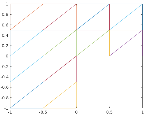
(a)

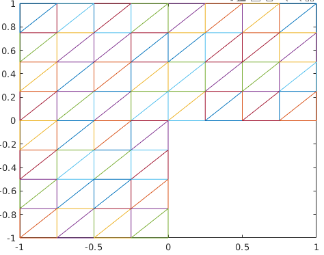
(b)

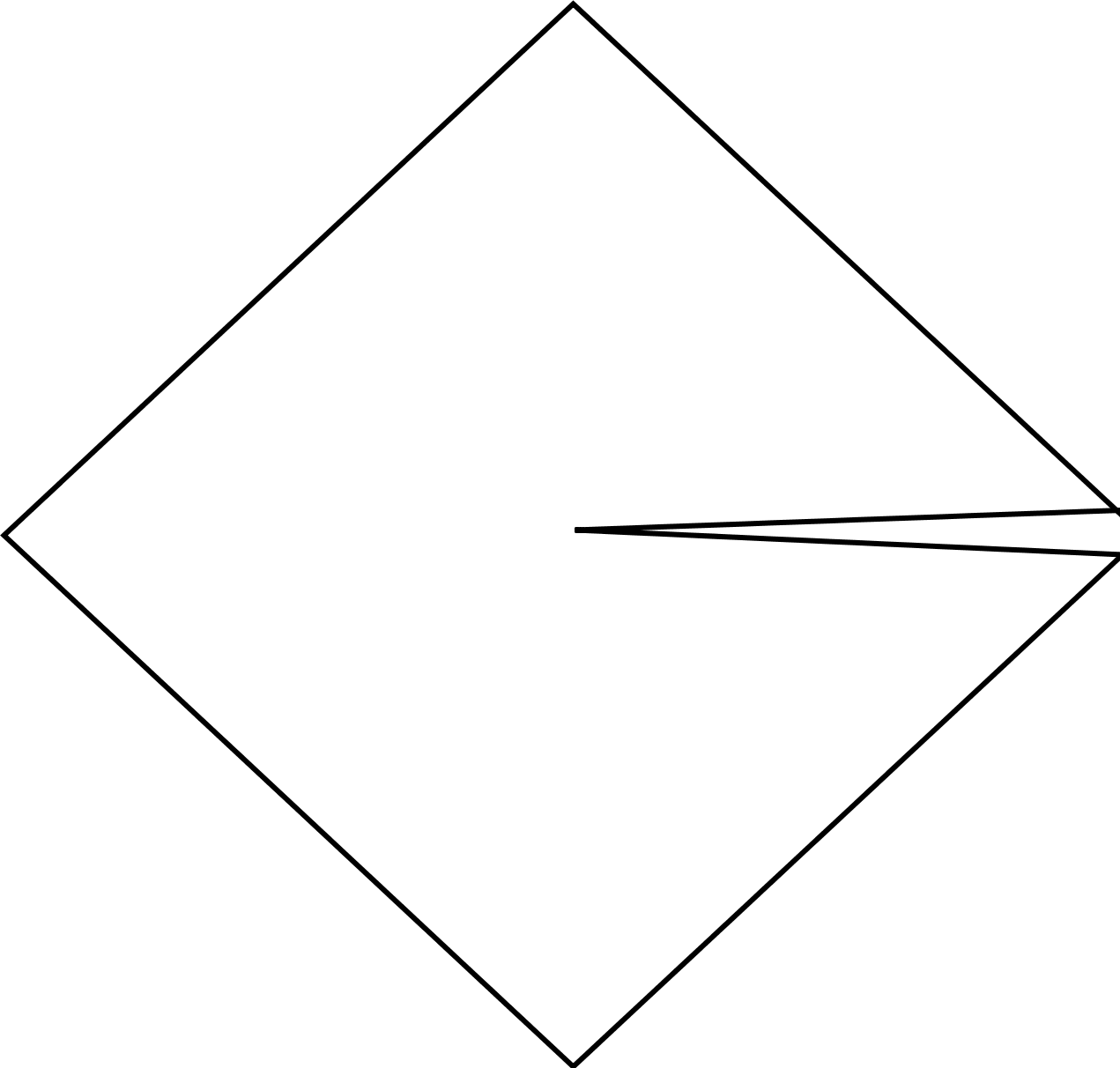
(c)

Figure 1: LABEL:sub@triangulation2Initial triangulation $\mathcal{T}_{0}$ of L-shape domain in Example 6.2 and LABEL:sub@triangulation3 its uniform refinement. LABEL:sub@Slit_domain Slit domain in Example 6.4

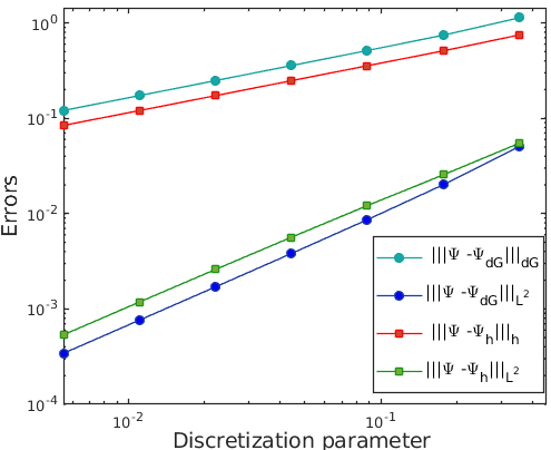
(a)

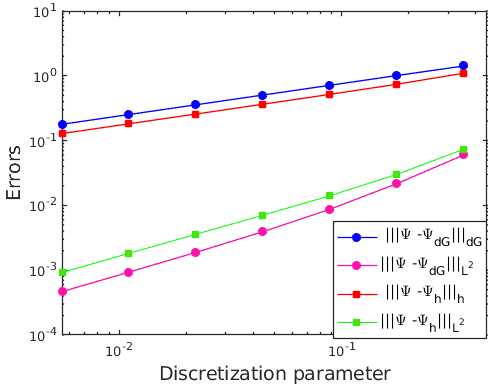
(b)

Figure 2: Convergence history (a priori estimates) for Nitsche’s method and dGFEM for LABEL:sub@Apriori_result_Lslape_domain Example 6.2, with $\epsilon=0.4$, and LABEL:sub@Apriori_result_Slit_domain Example 6.4, with $\epsilon=0.6$.

6.2 Example on a $L$-shaped domain

Consider (1.2) on a non-convex L-shape domain $\Omega=(-1,1)\times(-1,1)\setminus[0,1]\times[-1,0]$. For the manufactured solution $u=r^{{2}/{3}}\sin({2\theta}/{3}),$ $v=r^{1/2}\sin(\theta/2)$, where $(r,\theta)$ denote the system of polar coordinates, compute the corresponding right-hand side $\mathbf{f}$ and the non-homogeneous Dirichlet boundary condition $\mathbf{g}$. In this case, the exact solutions $\Psi\in\mathbf{H}^{1+1/2-\kappa}(\kappa\!>\!0)$ [14], and the theoretically expected rate of error reduction is $O(h^{1/2})$ and $O(h)$ in the energy norm and $\mathbf{L}^{2}$ norm (see Theorems 2.2 and 5.8). Figure 1a and 1b display the initial triangulation and its uniform refinement. The initial guess for the Nitsche’s method (resp. dGFEM) is chosen as $\Psi_{h}^{0}\in\mathbf{X}_{h}$ (resp. $\Psi_{\rm dG}^{0}\in\mathbf{X}_{{\rm dG}}$), where $\Psi_{h}^{0}$ solves $A_{h}(\Psi_{h}^{0},\Phi_{h})=L_{h}(\Phi_{h})\text{ for all }\Phi_{h}\in\mathbf{X}_{h}$ (resp. $A_{\rm dG}(\Psi_{\rm dG}^{0},\Phi_{\rm dG})=L_{\rm dG}(\Phi_{\rm dG})\text{ for all }\Phi_{\rm dG}\in\mathbf{X}_{{\rm dG}}$), and the linear form $L_{h}(\cdot)$ (resp. $L_{\rm dG}(\cdot)$) is modified to incorporate the information on $\mathbf{f}$. The approximations to the discrete solution to (2.3) are obtained using the Newton’s method defined in (6.1). Figure 2a presents the convergence rates in energy norm and $\mathbf{L}^{2}$ norm, with $\epsilon=0.4$, for both Nitsche’s method and dGFEM.

6.3 Benchmark example on unit square domain

Consider (2.1) on a convex domain $\Omega=(0,1)\times(0,1)$ with the Dirichlet boundary condition [22] given by $\displaystyle\mathbf{g}=\begin{cases}(\textit{T}_{d}(x),0)&\text{on}\,\,\,\,y=0\,\,\,\,\text{and}\,\,\,\,y=1\\ (-\textit{T}_{d}(y),0)&\text{on}\,\,\,\,x=0\,\,\,\,\text{and}\,\,\,\,x=1\end{cases}$, where the parameter $d=3\epsilon$ with $\epsilon=0.02$ and the trapezoidal shape function $\textit{T}_{d}:[0,1]\rightarrow{\mathbb{R}}$ is defined by $\displaystyle\textit{T}_{d}(t)=\begin{cases}t/d,&0\leq t\leq d\\ 1,&d\leq t\leq 1-d\\ (1-t)/d,&1-d\leq t\leq 1\end{cases}$. See [22, 24] for details of construction of a suitable initial guess of Newton’s iterates in this example.

$h$	Energy	${|\kern-1.07639pt|\kern-1.07639pt|\Psi_{h}^{n}-\Psi_{h}^{n-1}|\kern-1.07639pt|\kern-1.07639pt|}_{h}$	Order	${|\kern-1.07639pt|\kern-1.07639pt|\Psi_{h}^{n}-\Psi_{h}^{n-1}|\kern-1.07639pt|\kern-1.07639pt|}_{\mathbf{L}^{2}}$	Order
0.0220	79.2401782	1.84603412	-	0.92144678E-2	-
0.0110	78.2908458	0.93391985	0.98305855	0.29215012E-2	1.65719096
0.0055	78.0391327	0.46906124	0.99352244	0.85867723E-3	1.76652203
0.0027	77.9747996	0.23603408	0.99078112	0.22993326E-3	1.90090075
0.0220	87.9041386	1.86143892	-	0.95840689E-2	-
0.0110	86.9334857	0.94131381	0.98367059	0.29869842E-2	1.68194864
0.0055	86.6764846	0.47271729	0.99369812	0.87222395E-3	1.77591911
0.0027	86.6108341	0.23784715	0.99094285	0.23307142E-3	1.90392648

Table 1: Numerical energy, errors and convergence rates for D1 and R1 solutions, respectively in energy and $\mathbf{L}^{2}$ norms for $\epsilon=0.02$.

Table 1 presents the computed energy, error in energy and $\mathbf{L}^{2}$ norms for numerical approximation of the diagonal D1 and rotated R1 solutions, respectively obtained using the Nitsche’s method in (2.3). The orders of convergence agrees with the theoretical orders of convergence obtained in [22, 24, 33]. For the corresponding results for dGFEM, see [24, Tables 5, 6].

6.4 Example on a slit domain

Let $\Omega$ be the slit domain $\{(x,y)\in\mathbb{R}^{2}:|x|+|y|<1\}\setminus([0,1]\times\{0\})$ (see Figure 1c). Select the non-homogeneous Dirichlet boundary data $\mathbf{g}$ and the right-hand side $\mathbf{f}$ so that the manufactured solution is given by $u(r,\theta)=v(r,\theta)=r^{1/2}\sin(\theta/2)-(1/2)(r\sin(\theta))^{2}$. Figure 2b presents the convergence history in energy norm, $\mathbf{L}^{2}$ norm, with the parameter value $\epsilon=0.6$, for Nitsche’s method and dGFEM. The rates are approximately $0.5004$ (resp. $0.9846$) in energy norm ($\mathbf{L}^{2}$ norm).

6.5 Adaptive mesh-refinement

• For the adaptive refinement, the order of convergence of error and estimators are related to total number of unknowns ($\text{Ndof}(l)$). Let $e(l)$ and $\text{Ndof}(l)$ be the error and total number of unknowns at the $l-$th level refinement, respectively. The convergence rates are calculated as

  $$\text{Order}_{e}(l):=\frac{\log(e(l-1)/e(l))}{\log(\text{Ndof}(l)/\text{Ndof}(l-1))}\qquad\text{and}\qquad\text{Order}_{\vartheta}(l):=\frac{\log(\vartheta(l-1)/\vartheta(l))}{\log(\text{Ndof}(l)/\text{Ndof}(l-1))}.$$

• Given an initial triangulation $\mathcal{T}_{0},$ run the steps SOLVE, ESTIMATE, MARK and REFINE successively for different levels $l=0,1,2,\ldots$

  SOLVE Compute the solution $\Psi_{l}:=\Psi_{h}$ (resp. $\Psi_{l}:=\Psi_{\rm dG}$) of the discrete problem (2.3) (resp. 5.1) for the triangulation $\mathcal{T}_{l}$.

  ESTIMATE Calculate the error indicator $\displaystyle\varXi_{T,l}:=\big{(}\vartheta_{T}^{2}+\sum_{E\in\partial T\cap\mathcal{E}_{h}^{i}}(\vartheta^{i}_{E})^{2}+\sum_{E\in\partial T\cap\mathcal{E}_{h}^{\partial}}(\vartheta_{E}^{\partial})^{2}\big{)}^{\frac{1}{2}}$ for each element $T\in\mathcal{T}_{l}.$ Recall the volume and edge estimators for Nitsche’s method (resp. dGFEM) given by (2.4)-(2.5) (resp. (5.3)-(5.4)).

  MARK For next refinement, choose the elements $T\in\mathcal{T}_{l}$ using Dörfler marking such that $0.3\sum_{T\in{\mathcal{T}_{l}}}\varXi_{T,l}^{2}\\ \leq\sum_{T\in\tilde{\mathcal{T}}}\varXi_{T,l}^{2}$ and collect those elements to construct a subset $\tilde{\mathcal{T}}\subset\mathcal{T}_{l}$.

  REFINE Compute the closure of $\tilde{\mathcal{T}}$ and use newest vertex bisection [32] refinement strategy to construct the new triangulation $\mathcal{T}_{l+1}$.

Consider (1.2) in L-shaped domain (Figure 1a) with the manufactured solution presented in Example 6.2 and apply the adaptive refinement algorithm. The estimator is modified as $\vartheta_{T}^{2}:=h_{T}^{2}{|\kern-1.07639pt|\kern-1.07639pt|\mathbf{f}-2\epsilon^{-2}(|\Psi_{h}|^{2}-1)\Psi_{h}|\kern-1.07639pt|\kern-1.07639pt|}_{0,T}^{2}$ (resp. $\vartheta_{T}^{2}:=h_{T}^{2}{|\kern-1.07639pt|\kern-1.07639pt|\mathbf{f}-2\epsilon^{-2}(|\Psi_{\rm dG}|^{2}-1)\Psi_{\rm dG}|\kern-1.07639pt|\kern-1.07639pt|}_{0,T}^{2}$) for Nitsche’s method (resp. dGFEM) and this takes into account the effect of the non-zero right-hand side $\mathbf{f}$ calculated using the manufactured solution. Figures 3a and 3b (resp. Figures 3c and 3d) plot the discrete solutions, $u_{h}$ and $v_{h}$ of the Nitsche’s method (resp. dGFEM), respectively, with the parameter $\epsilon=0.4$, and display the adaptive refinement near the vicinity of the re-entrant corner of the L-shaped domain. Table 2 displays the computational error, estimator and convergence rates for uniform and adaptive mesh refinement for $\epsilon=0.4$. It is observed from Table 2 that we have a suboptimal empirical convergence rate (calculated with respect to Ndof) of $0.25$ for uniform mesh refinement and an improved optimal empirical convergence rate of $0.5$ for adaptive mesh-refinement. Further, in the adaptive refinement process, the number of mesh points required to achieve convergence is significantly reduced compared to uniform meshes and the convergence is faster than the uniform refinement process. Figure 4 displays the convergence behavior of the error and estimator along with the efficiency constant $C_{eff}$ plot, as a function of the total number of degrees of freedoms for $\epsilon=0.2,0.8$. Here, $C_{eff}$ is the ratio between computed estimators and errors, which remains constant after the first few refinement levels.

Figure 5 displays the discrete solutions (diagonal D1 and rotated R1) and the adaptive mesh refinements in the square domain $\Omega=(0,1)\times(0,1)$, for Example 6.3. Here, we observe adaptive mesh refinements near the defect points [22] of the domain (four corner points). Note that the estimator tends to zero as the number of degrees of freedom (Ndof) increases. Figure 6a (resp. Figure 6b) is the estimator vs Ndof plot for various values of $\epsilon$ for the diagonal, D1 solution obtained using Nitsche’s method (resp. dGFEM). The tolerance used for Newton’s method convergence is $10^{-6}$ and it is observed that for a fixed value of the discretization parameter $h$, the number of Newton iterations required for the convergence increases as the value of $\epsilon$ decreases. Observe that the rate of decay of the estimators is slower for smaller values of $\epsilon$ .

Remark 6.2.

The $h$-$\epsilon$ dependency, discussed in [24] has been reflected for adaptive refinement in this article, in terms of Ndof-$\epsilon$ dependency. It is observed in [24] that errors are sensitive to the choice of discretization parameter as $\epsilon$ decreases.

Figure 7a (resp. Figure 7b) display the discrete solution corresponding to the Example 6.4 and adaptive mesh-refinements, near the singularity at the origin for the parameter value $\epsilon=0.6$ (resp. $\epsilon=1$), for Nitsche’s method (resp. dGFEM). Figure 8a (resp. Figure 8b) shows the convergence history of errors in energy norm and estimators, for both uniform and adaptive refinements, for Nitsche’s method (resp. dGFEM). A sub-optimal empirical convergence rate $1/3$ for uniform refinement, and an improved empirical convergence rate $0.5$, for adaptive mesh refinement, are obtained as a function of degrees of freedom for both Nitsche’s method and dGFEM.

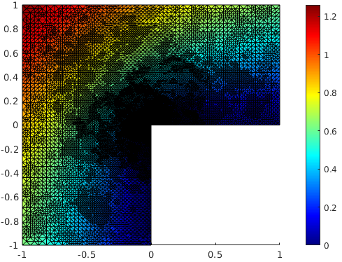
(a)

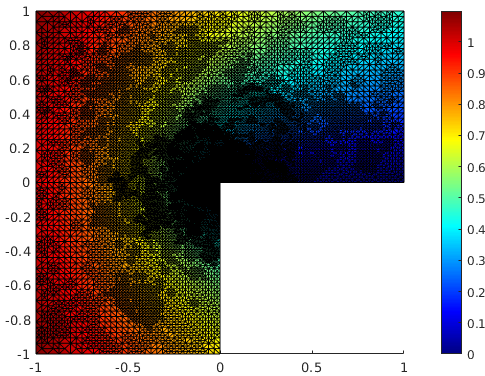
(b)

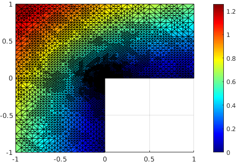
(c)

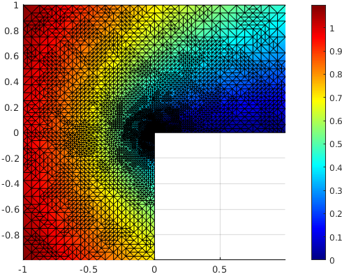
(d)

Figure 3: Adaptive mesh refinements: LABEL:sub@Exact_solution_uh $u_{h}$, LABEL:sub@Exact_solution_vh $v_{h}$ for Nitsche’s method and, LABEL:sub@Exact_solution_uh_dG $u_{h}$, LABEL:sub@Exact_solution_vh_dG $v_{h}$ for dGFEM for Example 6.2 with $\epsilon=0.4$.

Uniform refinement             Adaptive refinement
Ndof	Error	Ordere	$\vartheta$	Orderϑ		Ndof	Error	Ordere	$\vartheta$	Orderϑ
42	0.74880	-	2.14850	-		42	0.74880	-	2.14850	-
130	0.50988	0.3401	1.42668	0.3623		284	0.20381	0.6808	0.74811	0.5519
450	0.35592	0.2894	0.98209	0.3007		1298	0.07579	0.6509	0.34115	0.5167
1666	0.24796	0.2761	0.68290	0.2775		2958	0.04662	0.5899	0.22668	0.4962
6402	0.17274	0.2685	0.47546	0.2689		6732	0.02982	0.5434	0.15020	0.5004
25090	0.12053	0.2634	0.33121	0.2647		14792	0.01956	0.5356	0.10090	0.5053
99330	0.08426	0.2601	0.23099	0.2618		21936	0.01597	0.5146	0.08303	0.4945
395266	0.05902	0.2577	0.16138	0.2596		47326	0.01071	0.5194	0.05621	0.5074

Table 2: Numerical errors, estimators and experimental convergence rates for uniform and adaptive mesh refinement for $\epsilon=0.4.$

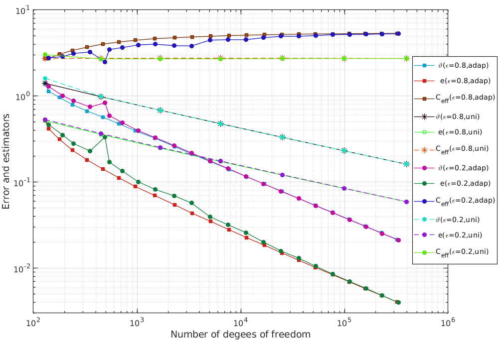
Figure 4: Ndof versus $e$, $\vartheta$ and $C_{eff}$ for L-shape domain in Example 6.2.

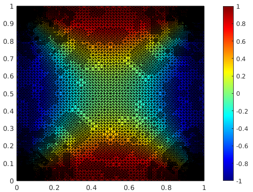
(a)

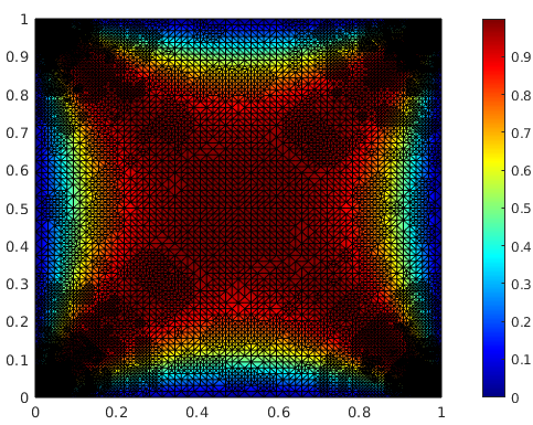
(b)

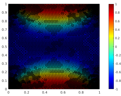
(c)

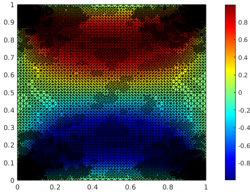
(d)

Figure 5: Adaptive mesh refinements: LABEL:sub@uD1 $u_{h}$, LABEL:sub@vD1 $v_{h}$ for D1 solution. Adaptive mesh refinements: LABEL:sub@uR1 $u_{h}$, LABEL:sub@vR1 $v_{h}$ for R1 solution of Example 6.3.

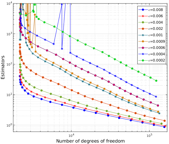
(a)

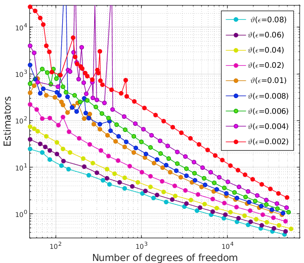
(b)

Figure 6: Ndof vs estimators plot for various values of $\epsilon$ in square domain Example 6.3 for LABEL:sub@Estimators Nitsche’s method and LABEL:sub@Estimators_dG dGFEM.

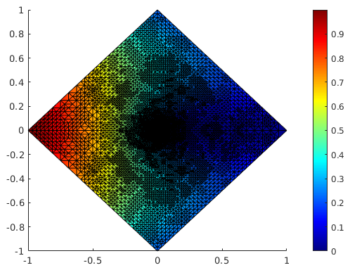
(a)

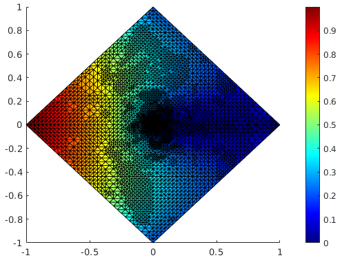
(b)

Figure 7: Adaptive mesh refinements: LABEL:sub@Slit_domain_triangulation_Nitsche $u_{h}$ for Nitsche’s method with $\epsilon=0.6$ . LABEL:sub@Slit_domain_triangulation_dG $u_{h}$ for dGFEM with $\epsilon$=$1.$

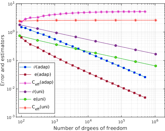
(a)

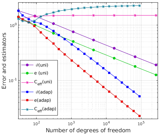
(b)

Figure 8: Ndof versus $e,$ $\vartheta$ and $C_{eff}$ for LABEL:sub@Slit_domain_Error_estimator_NitscheNitsche’s method with $\epsilon=0.6$ and LABEL:sub@Slit_domain_Error_estimator dGFEM with $\epsilon=1$.

7 Conclusions

This manuscript focuses on a priori and a posteriori error analysis for solutions with milder regularity than $\mathbf{H}^{2}$, and such solutions of lesser regularity are relevant, for example, in polygonal domains or domains with re-entrant corners that have boundary conditions of lesser regularity. We use Nitsche’s method for our analysis; the a priori error analysis relies on medius analysis and these techniques are extended to dGFEM. In [24], $h$-$\epsilon$ dependent error estimates for $\mathbf{H}^{2}(\Omega)$ regular solutions are obtained, and this follows from an $\epsilon$ independent bound for the exact solution ${|\kern-1.07639pt|\kern-1.07639pt|\Psi|\kern-1.07639pt|\kern-1.07639pt|}_{2}$, as established in [3]. It is not clear if such estimates are feasible for exact solutions with milder regularity, $\mathbf{H}^{1+\alpha}(\Omega),$ $0<\alpha\leq 1$, since we do not have $\epsilon$-independent bounds for ${|\kern-1.07639pt|\kern-1.07639pt|\Psi|\kern-1.07639pt|\kern-1.07639pt|}_{1+\alpha}$ at hand. It may be possible to obtain such bounds for certain model problems, which would allow $h-\epsilon$ dependent estimates. The methods in this paper will extend to modelling problems with weak anchoring or surface energies, which would translate to a Robin-type boundary condition; some dynamical models e.g. Allen-Cahn type evolution equations, stochastic versions of the Ginzburg-Landau system (1.2); modelling problems for composite material, such as ferronematics, which have both nematic and polar order etc. The overarching aim is to propose optimal estimates for the discretization parameter and number of degrees of freedom, for systems of second-order elliptic partial differential equations with lower order polynomial non-linearities, as a function of the model parameters e.g. $\epsilon$, and use these estimates for powerful new computational algorithms.

Appendix A Appendix

This section discusses the proofs of the local efficiency results in Lemmas 3.8-3.10. The local cut off functions play an important role to establish the local efficiency results. Consider the interior bubble function [1, 34] $\widehat{b}_{T}=27\widehat{\lambda}_{1}\widehat{\lambda}_{2}\widehat{\lambda}_{3}$ supported on a reference triangle $\widehat{T}$ with the barycentric coordinate functions $\widehat{\lambda}_{1},\widehat{\lambda}_{2},\widehat{\lambda}_{3}$. For $T\in\mathcal{T},$ let $\mathcal{F}_{T}:\widehat{T}\rightarrow T$ be a continuous, affine and invertible transformation. Define the bubble function on the element $T$ by $b_{T}=\widehat{b}_{T}\circ\mathcal{F}_{T}^{-1}$. Three edge bubble functions on the reference triangle $\widehat{T}$ are given by $\widehat{b}_{1}=4\widehat{\lambda}_{2}\widehat{\lambda}_{3}$, $\widehat{b}_{2}=4\widehat{\lambda}_{1}\widehat{\lambda}_{3}$ and $\widehat{b}_{3}=4\widehat{\lambda}_{1}\widehat{\lambda}_{2}$. On the edge $E$ of any triangle $T\in\mathcal{T}$, define the edge bubble function to be $b_{E}:=\widehat{b}_{E}\circ\mathcal{F}_{T}^{-1}$, where $\widehat{b}_{E}$ is the corresponding edge bubble function on $\widehat{T}$. Here, $b_{E}$ is supported on the pair of triangles sharing the edge $E.$

Lemma A.1.

[1, 34] Let $\widehat{P}\subset H^{1}(\widehat{T})$ be a finite dimensional subspace on the reference triangle $\widehat{T}$ and consider $P=\{\widehat{v}\circ\mathcal{F}_{T}^{-1}:\widehat{v}\in\widehat{P}\}$ to be the finite dimensional space of functions defined on $T$. Then the following inverse estimates hold for all $v\in P$,

$${|\kern-1.07639pt|v|\kern-1.07639pt|}^{2}_{L^{2}(T)}\lesssim\int_{T}b_{T}v^{2}\,{\rm dx}\lesssim{|\kern-1.07639pt|v|\kern-1.07639pt|}^{2}_{L^{2}(T)},\quad{|\kern-1.07639pt|v|\kern-1.07639pt|}_{L^{2}(T)}\lesssim{|\kern-1.07639pt|b_{T}v|\kern-1.07639pt|}_{L^{2}(T)}+h_{T}{|\kern-1.07639pt|\nabla(b_{T}v)|\kern-1.07639pt|}_{L^{2}(T)}\lesssim{|\kern-1.07639pt|v|\kern-1.07639pt|}_{L^{2}(T)}.$$ (A.1)

Let $E\subset\partial T$ be an edge and $b_{E}$ be the corresponding edge bubble function supported on the patch of triangles $\omega_{E}$ sharing the edge $E$. Let $P(E)$ be the finite dimensional space of functions defined on $E$ obtained by mapping $\widehat{P}(\widehat{E})\subset H^{1}(\widehat{E}).$ Then for all $v\in P(E)$,

$${|\kern-1.07639pt|v|\kern-1.07639pt|}^{2}_{L^{2}(E)}\lesssim\int_{E}b_{E}v^{2}\,{\rm dx}\lesssim{|\kern-1.07639pt|v|\kern-1.07639pt|}^{2}_{L^{2}(E)},\quad\,\,\,h_{E}^{-\frac{1}{2}}{|\kern-1.07639pt|b_{E}v|\kern-1.07639pt|}_{L^{2}(\omega_{E})}+h_{E}^{\frac{1}{2}}{|\kern-1.07639pt|\nabla(b_{E}v)|\kern-1.07639pt|}_{L^{2}(\omega_{E})}\lesssim{|\kern-1.07639pt|v|\kern-1.07639pt|}_{L^{2}(E)},$$ (A.2)

where the hidden constants in $"\lesssim"$ are independent of $h_{T}$ and $h_{E}$.

Proof of Lemma 3.8.

$(i)$ Let $T\in\mathcal{T}$ be arbitrary and $b_{T}$ be the interior bubble function supported on the triangle $T$. Choose $\displaystyle\boldsymbol{\rho}_{T}:=\left\{\begin{array}[]{l}\big{(}-\Delta\Phi_{h}+2\epsilon^{-2}(|\Phi_{h}|^{2}-1)\Phi_{h}\big{)}b_{T}\quad\text{in }T\\ 0\quad\text{in }\Omega\setminus T\end{array}\right.$, utilize (A.1), (2.1) with $\Phi:=\boldsymbol{\rho}_{T}$ and apply an integration by parts for the first term (which is a zero term) on the right-hand side below to obtain

$${|\kern-1.07639pt|\kern-1.07639pt|\boldsymbol{\eta}_{T}|\kern-1.07639pt|\kern-1.07639pt|}_{0,T}^{2}\lesssim\int_{T}\big{(}-\Delta\Phi_{h}+2\epsilon^{-2}(|\Phi_{h}|^{2}-1)\Phi_{h}\big{)}\cdot\boldsymbol{\rho}_{T}\,{\rm dx}$$

$$=A_{T}(\Phi_{h}-\Psi,\boldsymbol{\rho}_{T})+(B_{T}(\Phi_{h},\Phi_{h},\Phi_{h},\boldsymbol{\rho}_{T})-B_{T}(\Psi,\Psi,\Psi,\boldsymbol{\rho}_{T}))+C_{T}(\Phi_{h}-\Psi,\boldsymbol{\rho}_{T}).$$ (A.3)

Together with Hölder’s inequality, Lemma 3.6 and (A.1), the terms on the right-hand side of (A) are estimated as

$$A_{T}(\Phi_{h}-\Psi,\boldsymbol{\rho}_{T})\lesssim{|\kern-1.07639pt|\kern-1.07639pt|\nabla(\Phi_{h}-\Psi)|\kern-1.07639pt|\kern-1.07639pt|}_{0,T}{|\kern-1.07639pt|\kern-1.07639pt|\nabla\boldsymbol{\rho}_{T}|\kern-1.07639pt|\kern-1.07639pt|}_{0,T}\lesssim{|\kern-1.07639pt|\kern-1.07639pt|\Psi-\Phi_{h}|\kern-1.07639pt|\kern-1.07639pt|}_{1,T}h_{T}^{-1}{|\kern-1.07639pt|\kern-1.07639pt|\boldsymbol{\eta}_{T}|\kern-1.07639pt|\kern-1.07639pt|}_{0,T}.$$ (A.4)

$$C_{T}(\Phi_{h}-\Psi,\boldsymbol{\rho}_{T})\lesssim\epsilon^{-2}{|\kern-1.07639pt|\kern-1.07639pt|\Phi_{h}-\Psi|\kern-1.07639pt|\kern-1.07639pt|}_{0,T}{|\kern-1.07639pt|\kern-1.07639pt|\boldsymbol{\rho}_{T}|\kern-1.07639pt|\kern-1.07639pt|}_{0,T}\lesssim\epsilon^{-2}{|\kern-1.07639pt|\kern-1.07639pt|\Psi-\Phi_{h}|\kern-1.07639pt|\kern-1.07639pt|}_{0,T}{|\kern-1.07639pt|\kern-1.07639pt|\boldsymbol{\eta}_{T}|\kern-1.07639pt|\kern-1.07639pt|}_{0,T},$$ (A.5)

$$B_{T}(\Phi_{h},\Phi_{h},\Phi_{h},\boldsymbol{\rho}_{T})-B_{T}(\Psi,\Psi,\Psi,\boldsymbol{\rho}_{T})\lesssim \epsilon^{-2}{|\kern-1.07639pt|\kern-1.07639pt|\Psi-\Phi_{h}|\kern-1.07639pt|\kern-1.07639pt|}_{1,T}({|\kern-1.07639pt|\kern-1.07639pt|\Psi-\Phi_{h}|\kern-1.07639pt|\kern-1.07639pt|}_{1,T}({|\kern-1.07639pt|\kern-1.07639pt|\Phi_{h}|\kern-1.07639pt|\kern-1.07639pt|}_{1,T}+{|\kern-1.07639pt|\kern-1.07639pt|\Psi|\kern-1.07639pt|\kern-1.07639pt|}_{1,T})$$

$$+{|\kern-1.07639pt|\kern-1.07639pt|\Psi|\kern-1.07639pt|\kern-1.07639pt|}_{1,T}^{2})h_{T}^{-1}{|\kern-1.07639pt|\kern-1.07639pt|\boldsymbol{\eta}_{T}|\kern-1.07639pt|\kern-1.07639pt|}_{0,T}.$$ (A.6)

A combination of the above three displayed estimates in (A) plus Lemma A.1 establishes

$$h_{T}{|\kern-1.07639pt|\kern-1.07639pt|\boldsymbol{\eta}_{T}|\kern-1.07639pt|\kern-1.07639pt|}_{0,T}\lesssim{|\kern-1.07639pt|\kern-1.07639pt|\Psi-\Phi_{h}|\kern-1.07639pt|\kern-1.07639pt|}_{h,T}(1+\epsilon^{-2}(1+{|\kern-1.07639pt|\kern-1.07639pt|\Psi|\kern-1.07639pt|\kern-1.07639pt|}_{1,T}^{2}+{|\kern-1.07639pt|\kern-1.07639pt|\Psi-\Phi_{h}|\kern-1.07639pt|\kern-1.07639pt|}_{h,T}({|\kern-1.07639pt|\kern-1.07639pt|\Phi_{h}|\kern-1.07639pt|\kern-1.07639pt|}_{1,T}+{|\kern-1.07639pt|\kern-1.07639pt|\Psi|\kern-1.07639pt|\kern-1.07639pt|}_{1,T}))).$$ (A.7)

To find the estimate corresponding to $\boldsymbol{\eta}_{E}$, consider the edge bubble function $b_{E}$ supported on the patch of triangles $\omega_{E}$ sharing the edge $E$. Define $\displaystyle\boldsymbol{\rho}_{E}:=\left\{\begin{array}[]{l}[\nabla\Phi_{h}\nu]b_{E}\quad\text{in }\omega_{E}\\ 0\quad\text{in }\Omega\setminus\omega_{E}\end{array}\right.$ and use (A.2), $[\boldsymbol{\rho}_{E}]=0$ for $E\in\mathcal{E}_{h}^{i}$ and an integration by parts to obtain

$${|\kern-1.07639pt|\kern-1.07639pt|\boldsymbol{\eta}_{E}|\kern-1.07639pt|\kern-1.07639pt|}_{0,E}^{2} \lesssim\int_{E}[\nabla\Phi_{h}\nu]\cdot\boldsymbol{\rho}_{E}\,{\rm ds}=\int_{E}[\nabla\Phi_{h}\nu]\cdot\{\ \boldsymbol{\rho}_{E}\}\,{\rm ds}+\int_{E}\{\nabla\Phi_{h}\nu\}\cdot[\boldsymbol{\rho}_{E}]\,{\rm ds}$$

$$=\sum_{T\in\omega_{E}}\int_{T}(\Delta\Phi_{h}\cdot\boldsymbol{\rho}_{E}+\nabla\Phi_{h}\cdot\nabla\boldsymbol{\rho}_{E})\,{\rm dx}.$$ (A.8)

Add and subtract $\sum_{T\in\omega_{E}}\int_{T}2\epsilon^{-2}(|\Phi_{h}|^{2}-1)\Phi_{h}\cdot\boldsymbol{\rho}_{E}\,{\rm dx}$ in the right-hand side of (A) to rewrite the expression with the help of $\boldsymbol{\eta}_{T}=\Delta\Phi_{h}-2\epsilon^{-2}(|\Phi_{h}|^{2}-1)\Phi_{h}$ (with a $-\Delta\Phi_{h}=0$ added). The expression (2.1) with $\Phi=\boldsymbol{\rho}_{E}$, a re-grouping of terms and Hölder’s inequality lead to

$${|\kern-1.07639pt|\kern-1.07639pt|\boldsymbol{\eta}_{E}|\kern-1.07639pt|\kern-1.07639pt|}_{0,E}^{2} \lesssim(\sum_{T\in\omega_{E}}{|\kern-1.07639pt|\kern-1.07639pt|\boldsymbol{\eta}_{T}|\kern-1.07639pt|\kern-1.07639pt|}_{0,T}^{2})^{\frac{1}{2}}(\sum_{T\in\omega_{E}}{|\kern-1.07639pt|\kern-1.07639pt|\boldsymbol{\rho}_{E}|\kern-1.07639pt|\kern-1.07639pt|}_{0,T}^{2})^{\frac{1}{2}}+\sum_{T\in\omega_{E}}(A_{T}(\Phi_{h}-\Psi,\boldsymbol{\rho}_{E})+C_{T}(\Phi_{h}-\Psi,\boldsymbol{\rho}_{E})$$

$$\quad+(B_{T}(\Phi_{h},\Phi_{h},\Phi_{h},\boldsymbol{\rho}_{E})-B_{T}(\Psi,\Psi,\Psi,\boldsymbol{\rho}_{E}))).$$ (A.9)

A combination of Hölder’s inequality, Lemma 3.6 and (A.2) yields

$$\sum_{T\in\omega_{E}}A_{T}(\Phi_{h}-\Psi,\boldsymbol{\rho}_{E})\lesssim\sum_{T\in\omega_{E}}{|\kern-1.07639pt|\kern-1.07639pt|\nabla(\Psi-\Phi_{h})|\kern-1.07639pt|\kern-1.07639pt|}_{0,T}{|\kern-1.07639pt|\kern-1.07639pt|\nabla\boldsymbol{\rho}_{E}|\kern-1.07639pt|\kern-1.07639pt|}_{0,T}\lesssim h_{E}^{-\frac{1}{2}}{|\kern-1.07639pt|\kern-1.07639pt|\boldsymbol{\eta}_{E}|\kern-1.07639pt|\kern-1.07639pt|}_{0,E}{|\kern-1.07639pt|\kern-1.07639pt|\nabla(\Psi-\Phi_{h})|\kern-1.07639pt|\kern-1.07639pt|}_{0,\omega_{E}},$$ (A.10)

$$\sum_{T\in\omega_{E}}C_{T}(\Phi_{h}-\Psi,\boldsymbol{\rho}_{E})\lesssim\epsilon^{-2}\sum_{T\in\omega_{E}}{|\kern-1.07639pt|\kern-1.07639pt|\Psi-\Phi_{h}|\kern-1.07639pt|\kern-1.07639pt|}_{0,T}{|\kern-1.07639pt|\kern-1.07639pt|\boldsymbol{\rho}_{E}|\kern-1.07639pt|\kern-1.07639pt|}_{0,T}\lesssim\epsilon^{-2}h_{E}^{\frac{1}{2}}{|\kern-1.07639pt|\kern-1.07639pt|\boldsymbol{\eta}_{E}|\kern-1.07639pt|\kern-1.07639pt|}_{0,E}{|\kern-1.07639pt|\kern-1.07639pt|\Psi-\Phi_{h}|\kern-1.07639pt|\kern-1.07639pt|}_{0,\omega_{E}},$$ (A.11)

$$\sum_{T\in\omega_{E}}(B_{T}(\Phi_{h},\Phi_{h},\Phi_{h},\boldsymbol{\rho}_{E})-B_{T}(\Psi,\Psi,\Psi,\boldsymbol{\rho}_{E}))\lesssim \epsilon^{-2}h_{E}^{-\frac{1}{2}}{|\kern-1.07639pt|\kern-1.07639pt|\boldsymbol{\eta}_{E}|\kern-1.07639pt|\kern-1.07639pt|}_{0,E}\sum_{T\in\omega_{E}}{|\kern-1.07639pt|\kern-1.07639pt|\Psi-\Phi_{h}|\kern-1.07639pt|\kern-1.07639pt|}_{1,T}({|\kern-1.07639pt|\kern-1.07639pt|\Psi-\Phi_{h}|\kern-1.07639pt|\kern-1.07639pt|}_{1,T}({|\kern-1.07639pt|\kern-1.07639pt|\Phi_{h}|\kern-1.07639pt|\kern-1.07639pt|}_{1,T}$$

$$+{|\kern-1.07639pt|\kern-1.07639pt|\Psi|\kern-1.07639pt|\kern-1.07639pt|}_{1,T})+{|\kern-1.07639pt|\kern-1.07639pt|\Psi|\kern-1.07639pt|\kern-1.07639pt|}_{1,T}^{2}).$$ (A.12)

The estimate of ${|\kern-1.07639pt|\kern-1.07639pt|\boldsymbol{\eta}_{T}|\kern-1.07639pt|\kern-1.07639pt|}_{0,T}$ in (A.7) and (A.2) together with the above three displayed estimates in (A) lead to

$$h_{E}^{\frac{1}{2}}{|\kern-1.07639pt|\kern-1.07639pt|\boldsymbol{\eta}_{E}|\kern-1.07639pt|\kern-1.07639pt|}_{0,E}\lesssim\sum_{T\in\omega_{E}}{|\kern-1.07639pt|\kern-1.07639pt|\Psi-\Phi_{h}|\kern-1.07639pt|\kern-1.07639pt|}_{h,T}(1+\epsilon^{-2}(1+{|\kern-1.07639pt|\kern-1.07639pt|\Psi|\kern-1.07639pt|\kern-1.07639pt|}_{1,T}^{2}+{|\kern-1.07639pt|\kern-1.07639pt|\Psi-\Phi_{h}|\kern-1.07639pt|\kern-1.07639pt|}_{h,T}({|\kern-1.07639pt|\kern-1.07639pt|\Phi_{h}|\kern-1.07639pt|\kern-1.07639pt|}_{1}+{|\kern-1.07639pt|\kern-1.07639pt|\Psi|\kern-1.07639pt|\kern-1.07639pt|}_{1,T}))).$$ (A.13)

A combination of (A.7) and A.13 completes the proof of $(i)$ in Lemma 3.8.

$(ii)$ For $\Phi_{h}={\rm I}_{h}\Psi$ in (A.6), Lemma 3.6$(v)$ and (A.1) yield

$$B_{T}({\rm I}_{h}\Psi,{\rm I}_{h}\Psi,{\rm I}_{h}\Psi,\boldsymbol{\rho}_{T})-B_{T}(\Psi,\Psi,\Psi,\boldsymbol{\rho}_{T}) \lesssim\epsilon^{-2}{|\kern-1.07639pt|\kern-1.07639pt|\Psi|\kern-1.07639pt|\kern-1.07639pt|}_{1+\alpha,T}^{3}(h_{T}^{2\alpha}{|\kern-1.07639pt|\kern-1.07639pt|\nabla\boldsymbol{\rho}_{T}|\kern-1.07639pt|\kern-1.07639pt|}_{0,T}+h_{T}^{1+\alpha}{|\kern-1.07639pt|\kern-1.07639pt|\boldsymbol{\rho}_{T}|\kern-1.07639pt|\kern-1.07639pt|}_{0,T})$$

$$\lesssim\epsilon^{-2}{|\kern-1.07639pt|\kern-1.07639pt|\Psi|\kern-1.07639pt|\kern-1.07639pt|}_{1+\alpha,T}^{3}(h_{T}^{2\alpha}+h_{T}^{2+\alpha})h_{T}^{-1}{|\kern-1.07639pt|\kern-1.07639pt|\boldsymbol{\eta}_{T}|\kern-1.07639pt|\kern-1.07639pt|}_{0,T}.$$ (A.14)

Substitute (A.4), (A.5), (A) in (A) and utilize Lemma 3.3 to arrive at

$$h_{T}{|\kern-1.07639pt|\kern-1.07639pt|\boldsymbol{\eta}_{T}|\kern-1.07639pt|\kern-1.07639pt|}_{0,T} \lesssim{|\kern-1.07639pt|\kern-1.07639pt|\nabla({\rm I}_{h}\Psi-\Psi)|\kern-1.07639pt|\kern-1.07639pt|}_{0,T}+\epsilon^{-2}{|\kern-1.07639pt|\kern-1.07639pt|{\rm I}_{h}\Psi-\Psi|\kern-1.07639pt|\kern-1.07639pt|}_{0,T}+\epsilon^{-2}h_{T}^{2\alpha}{|\kern-1.07639pt|\kern-1.07639pt|\Psi|\kern-1.07639pt|\kern-1.07639pt|}_{1+\alpha}^{3}$$

$$\lesssim h_{T}^{\alpha}(1+\epsilon^{-2}h_{T}^{\alpha}(1+{|\kern-1.07639pt|\kern-1.07639pt|\Psi|\kern-1.07639pt|\kern-1.07639pt|}_{1+\alpha}^{2})){|\kern-1.07639pt|\kern-1.07639pt|\Psi|\kern-1.07639pt|\kern-1.07639pt|}_{1+\alpha}.$$ (A.15)

A choice of $\Phi_{h}={\rm I}_{h}\Psi$ in (A), Lemma 3.6$(v)$ and (A.2) yield

$$\sum_{T\in\omega_{E}}(B_{T}({\rm I}_{h}\Psi,{\rm I}_{h}\Psi,{\rm I}_{h}\Psi,\boldsymbol{\rho}_{E})-B_{T}(\Psi,\Psi,\Psi,\boldsymbol{\rho}_{E}))\lesssim\epsilon^{-2}\sum_{T\in\omega_{E}}{|\kern-1.07639pt|\kern-1.07639pt|\Psi|\kern-1.07639pt|\kern-1.07639pt|}_{1+\alpha,T}^{3}(h_{T}^{2\alpha}{|\kern-1.07639pt|\kern-1.07639pt|\nabla\boldsymbol{\rho}_{E}|\kern-1.07639pt|\kern-1.07639pt|}_{0,T}+h_{T}^{1+\alpha}{|\kern-1.07639pt|\kern-1.07639pt|\boldsymbol{\rho}_{E}|\kern-1.07639pt|\kern-1.07639pt|}_{0,T})$$

$$\qquad\lesssim\epsilon^{-2}h_{E}^{-\frac{1}{2}}{|\kern-1.07639pt|\kern-1.07639pt|\boldsymbol{\eta}_{E}|\kern-1.07639pt|\kern-1.07639pt|}_{0,E}\sum_{T\in\omega_{E}}{|\kern-1.07639pt|\kern-1.07639pt|\Psi|\kern-1.07639pt|\kern-1.07639pt|}_{1+\alpha,T}^{3}(h_{T}^{2\alpha}+h_{E}h_{T}^{2+\alpha}).$$ (A.16)

Substitute (A.10), (A.11), (A) in (A) and employ Lemma 3.3 to obtain

$$h_{E}^{\frac{1}{2}}{|\kern-1.07639pt|\kern-1.07639pt|\boldsymbol{\eta}_{E}|\kern-1.07639pt|\kern-1.07639pt|}_{0,E}\lesssim\sum_{T\in\omega_{E}}h_{T}^{\alpha}(1+\epsilon^{-2}h_{T}^{\alpha}(1+{|\kern-1.07639pt|\kern-1.07639pt|\Psi|\kern-1.07639pt|\kern-1.07639pt|}_{1+\alpha}^{2})){|\kern-1.07639pt|\kern-1.07639pt|\Psi|\kern-1.07639pt|\kern-1.07639pt|}_{1+\alpha}.$$ (A.17)

A combination of (A) and (A.17) concludes the proof of $(ii)$ in Lemma 3.8. ∎

The proof of Lemma 3.9 (resp. 3.10) follows analgous to the proof of Lemma 3.8 with the choice of

$$\boldsymbol{\rho}_{T}:=\left\{\begin{array}[]{ll@{:}}(\Delta(\textrm{I}_{h}\boldsymbol{\xi})+2\epsilon^{-2}(|\textrm{I}_{h}\Psi|^{2}\Theta_{h}+2(\textrm{I}_{h}\Psi\cdot\Theta_{h})\textrm{I}_{h}\Psi-\Theta_{h}))b_{T}\text{ in }T\\ 0\quad\text{in }\Omega\setminus T\end{array}\right.\text{ and }\boldsymbol{\rho}_{E}:=\left\{\begin{array}[]{l}[\nabla(\textrm{I}_{h}\boldsymbol{\xi})\nu]b_{E}\text{ in }\omega_{E}\\ 0\quad\text{in }\Omega\setminus\omega_{E}\end{array}\right..$$

$$\bigg{(}\text{resp. }\boldsymbol{\rho}_{T}:=\left\{\begin{array}[]{l}\big{(}G_{h}+\Delta(\textrm{I}_{h}\boldsymbol{\chi})-2\epsilon^{-2}(|\textrm{I}_{h}\Psi|^{2}\textrm{I}_{h}\boldsymbol{\chi}+2(\textrm{I}_{h}\Psi\cdot\textrm{I}_{h}\boldsymbol{\chi})\textrm{I}_{h}\Psi-\textrm{I}_{h}\boldsymbol{\chi})\big{)}b_{T}\quad\text{in }T\\ 0\quad\text{in }\Omega\setminus T\end{array}\right.$$

$$\text{ and }\boldsymbol{\rho}_{E}:=\left\{\begin{array}[]{l}[\nabla(\textrm{I}_{h}\boldsymbol{\chi})\nu]b_{E}\quad\text{in }\omega_{E}\\ 0\quad\text{in }\Omega\setminus\omega_{E}\end{array}\right.\bigg{)}.$$

References

- [1] M. Ainsworth and J. T. Oden, A posteriori error estimation in finite element analysis, Pure and Applied Mathematics (New York), Wiley-Interscience [John Wiley & Sons], New York, 2000.
- [2] S. Bartels, C. Carstensen, and G. Dolzmann, Inhomogeneous Dirichlet conditions in a priori and a posteriori finite element error analysis, Numerische Mathematik 99 (2004), no. 1, 1–24.
- [3] F. Bethuel, H. Brezis, and F. Hélein, Asymptotics for the minimization of a Ginzburg-Landau functional, Calculus of Variations and Partial Differential Equations 1 (1993), no. 2, 123–148.
- [4] , Ginzburg-Landau vortices, Progress in Nonlinear Differential Equations and their Applications, vol. 13, Birkhäuser Boston, Inc., Boston, MA, 1994.
- [5] D. Braess and R. Verfürth, A posteriori error estimators for the Raviart-Thomas element, SIAM Journal on Numerical Analysis 33 (1996), no. 6, 2431–2444.
- [6] S. C. Brenner, Poincaré-Friedrichs inequalities for piecewise functions, SIAM Journal on Numerical Analysis 41 (2003), no. 1, 306–324.
- [7] C. Carstensen, R. Lazarov, and S. Tomov, Explicit and averaging a posteriori error estimates for adaptive finite volume methods, SIAM Journal on Numerical Analysis 42 (2005), no. 6, 2496–2521.
- [8] C. Carstensen, G. Mallik, and N. Nataraj, A priori and a posteriori error control of discontinuous Galerkin finite element methods for the von Kármán equations, IMA J. Numer. Anal. 39 (2019), no. 1, 167–200.
- [9] , Nonconforming finite element discretisation for semilinear problems with trilinear nonlinearity, (2019).
- [10] P. G. Ciarlet, The finite element method for elliptic problems, Classics in Applied Mathematics, vol. 40, Society for Industrial and Applied Mathematics (SIAM), Philadelphia, PA, 2002.
- [11] P.G. de Gennes and J. Prost, The physics of liquid crystals, International Series of Monogr, Clarendon Press, 1993.
- [12] D. A. Di Pietro and A. Ern, Mathematical aspects of discontinuous Galerkin methods, Mathématiques & Applications (Berlin) [Mathematics & Applications], vol. 69, Springer, Heidelberg, 2012.
- [13] D. Golovaty, J. A. Montero, and P. Sternberg, Dimension reduction for the Landau-de Gennes model in planar nematic thin films, Journal of Nonlinear Science 25 (2015), no. 6, 1431–1451.
- [14] P. Grisvard, Singularities in boundary value problems, Recherches en Mathématiques Appliquées [Research in Applied Mathematics], vol. 22, Masson, Paris; Springer-Verlag, Berlin, 1992.
- [15] T. Gudi, A new error analysis for discontinuous finite element methods for linear elliptic problems, Mathematics of Computation 79 (2010), no. 272, 2169–2189.
- [16] D. Henao, A. Majumdar, and A. Pisante, Uniaxial versus biaxial character of nematic equilibria in three dimensions, Calculus of Variations and Partial Differential Equations 56 (2017), no. 2, Art. 55, 22.
- [17] M. Juntunen and R. Stenberg, Nitsche’s method for general boundary conditions, Mathematics of Computation 78 (2009), no. 267, 1353–1374.
- [18] O. A. Karakashian and F. Pascal, A posteriori error estimates for a discontinuous Galerkin approximation of second-order elliptic problems, SIAM Journal on Numerical Analysis 41 (2003), no. 6, 2374–2399.
- [19] K. Y. Kim, A posteriori error analysis for locally conservative mixed methods, Mathematics of Computation 76 (2007), no. 257, 43–66.
- [20] , A posteriori error estimators for locally conservative methods of nonlinear elliptic problems, Applied Numerical Mathematics. An IMACS Journal 57 (2007), no. 9, 1065–1080.
- [21] A. Lasis and E. Süli, Poincaré-type inequalities for broken obolev spaces, Technical Report 03/10, Oxford University Computing Laboratory, Oxford, England (2003).
- [22] C. Luo, A. Majumdar, and R. Erban, Multistability in planar liquid crystal wells, Physics Review E 85 (2012), 061702.
- [23] N. Lüthen, M. Juntunen, and R. Stenberg, An improved a priori error analysis of Nitsche’s method for Robin boundary conditions, Numer. Math. 138 (2018), no. 4, 1011–1026.
- [24] R. R. Maity, A. Majumdar, and N. Nataraj, Discontinuous Galerkin finite element methods for the Landau-de Gennes minimization problem of liquid crystals, IMA Journal of Numerical Analysis (2020).
- [25] A. Majumdar, Equilibrium order parameters of nematic liquid crystals in the Landau-de Gennes theory, European Journal of Applied Mathematics 21 (2010), no. 2, 181–203.
- [26] A. Majumdar and A. Zarnescu, Landau-de Gennes theory of nematic liquid crystals: the Oseen-Frank limit and beyond, Archive for Rational Mechanics and Analysis 196 (2010), no. 1, 227–280.
- [27] J. Nitsche, Über ein variationsprinzip zur lösung von dirichlet-problemen bei verwendung von teilräumen, die keinen randbedingungen unterworfen sind, Abhandlungen aus dem Mathematischen Seminar der Universität Hamburg 36 (1971), no. 1, 9–15.
- [28] F. Pacard and T. Rivière, Linear and nonlinear aspects of vortices: The Ginzburg-Landau model, Progress in Nonlinear Differential Equations and Their Applications, Birkhäuser, 2000.
- [29] S. Prudhomme, F. Pascal, J. T. Oden, and A. Romkes, A priori error estimate for the Baumann-Oden version of the discontinuous Galerkin method, Comptes Rendus de l’Académie des Sciences. Série I. Mathématique 332 (2001), no. 9, 851–856.
- [30] F. Pascal S. Prudhomme and J.T. Oden, Review of error estimation for discontinuous galerkin method, TICAM-report 00-27, The university of Texas at Austin (2000).
- [31] L. R. Scott and S. Zhang, Finite element interpolation of nonsmooth functions satisfying boundary conditions, Mathematics of Computation 54 (1990), no. 190, 483–493.
- [32] R. Stevenson, The completion of locally refined simplicial partitions created by bisection, Math. Comp. 77 (2008), no. 261, 227–241.
- [33] C. Tsakonas, A. J. Davidson, C. V. Brown, and N. J. Mottram, Multistable alignment states in nematic liquid crystal filled wells, Applied Physics Letters 90 (2007), Article 111913.
- [34] R. Verfürth, A posteriori error estimation techniques for finite element methods, Numerical Mathematics and Scientific Computation, Oxford University Press, Oxford, 2013.
- [35] Y. Wang, G. Canevari, and A. Majumdar, Order reconstruction for nematics on squares with isotropic inclusions: a Landau–de Gennes study, SIAM J. Appl. Math. 79 (2019), no. 4, 1314–1340.