Maximal extension of the Schwarzschild metric: From Painlevé-Gullstrand to Kruskal-Szekeres

Abstract

We find a specific coordinate system that goes from the Painlevé-Gullstrand partial extension to the Kruskal-Szekeres maximal extension and thus exhibit the maximal extension of the Schwarzschild metric in a unified picture. We do this by adopting two time coordinates, one being the proper time of a congruence of outgoing timelike geodesics, the other being the proper time of a congruence of ingoing timelike geodesics, both parameterized by the same energy per unit mass $E$. $E$ is in the range $1\leq E<\infty$ with the limit $E=\infty$ yielding the Kruskal-Szekeres maximal extension. So, through such an integrated description one sees that the Kruskal-Szekeres solution belongs to this family of extensions parameterized by $E$. Our family of extensions is different from the Novikov-Lemaître family parameterized also by the energy $E$ of timelike geodesics, with the Novikov extension holding for $0<E<1$ and being maximal, and the Lemaître extension holding for $1\leq E<\infty$ and being partial, not maximal, and moreover its $E=\infty$ limit evanescing in a Minkowski spacetime rather than ending in the Kruskal-Szekeres spacetime.

I Introduction

The maximal analytical extension of the Schwarzschild solution was a remarkable achievement in general relativity and in the theory of black holes. For the first time the complex causal structure with a convoluted spacetime topology, stemming from the seemingly trivial generalization into general relativity of a point particle attractor in Newtonian gravitation, was unfolded.

It all started with the spherically symmetric vacuum solution of general relativity found by Schwarzschild schwarzschild , that was put in different terms and in a somewhat different coordinate system by Droste droste and Hilbert hilbert , and shown to be unique by Birkhoff birkhoff . Leaving aside Schwarzschild’s interpretation of Schwarzschild’s solution, it is the solution that later gave rise to black holes. To finalize its full meaning it was necessary to understand the sphere $r=2M$ that naturally appears in the solution and accomplish its maximal extension, i.e., finding the corresponding spacetime in which every geodesic originating from an arbitrary point in it has infinite length in both directions or ends at a singularity that cannot be removed by a coordinate transformation. These were two problems that proved difficult.

An early attempt to eliminate the $r=2M$ sphere obstacle and its inside was provided by Einstein and Rosen er that tried to join smoothly at $r=2M$ two distinct spacetime sheets in order to get some kind of fundamental particle, in what is known as an Einstein-Rosen bridge. Misner and Wheeler misnerwheeler generalized the bridge into a wormhole with a throat at its maximum opening. Wormholes became a focus of study within general relativity after Morris and Thorne thornemorris showed that with some suitable form of matter, albeit exotic, they could be traversable, see also, e.g., the work of Lemos, Lobo and Oliveira lemoslq . The Einstein-Rosen bridge in terms of the understanding of the $r=2M$ sphere was a dead end, but as a nontraversable wormhole it reincarnated in the maximal extensions of the Schwarzschild metric, and as a traversable wormhole it can be put in firm ground once one properly defines it in order to have an admissible matter support, as disclosed by Guendelman, Nissimov, Pacheva, and Stoilov guendelman .

A promising way of seeing the Schwarzschild solution, whatever the motivation, came with Painlevé painleve that changed the Schwarzschild time coordinate into the proper time of a congruence of ingoing timelike geodesics, or equivalently of ingoing test particles planted over them, with energy per unit mass $E$ equal to one, that admitted to put the line element in a new form that was not singular at $r=2M$. This procedure was also discovered by Gullstrand gullstrand , and the resulting line element, which works as for outgoing as for ingoing timelike geodesics, is called the Painlevé-Gullstrand line element of the Schwarzschild solution, or simply referred as Painlevé-Gullstrand solution, and in both forms it is an analytical extension, although partial, of the original Schwarzschild solution. The generalization of this line element to accommodate a congruence of timelike geodesics with any $E$, less or greater than one, was given by Gautreau and Hoffmann gautreauhoffmann . The Painlevé-Gullstrand line element, not being singular at $r=2M$, is useful in many understandings of black hole physics. For instance, it has been used by Parikh and Wilczek to understand how Hawking radiation proceeds parikhwilczek , or as a guide for a better understanding of the $r=2M$ sphere by Martel and Poisson martelpoisson , or to understand in new ways the Kerr metric by Natário natario , or as a generalized slicing of the Schwarzschild spacetime by Finch finch and MacLaurin maclaurin2019 .

An extension of the Painlevé-Gullstrand line element was given by Lemaître lemaitre that transformed the time and radial coordinates of the Schwarzschild solution to the proper time of ingoing timelike geodesics with $E=1$ and to a suitable new comoving radial coordinate, and showed in a stroke that $r=2M$ was a fine sphere, with nothing singular about it, performing thus an analytical extension, although partial, of the Schwarzschild solution. Novikov novikov understood that for timelike geodesics with $0<E<1$ it was possible to perform a maximal analytical extension and display the Schwarzschild solution in its fullness. The Lemaître extension, as an exterior spacetime, was implicitly used in the gravitational contraction of a cloud of dust by Oppenheimer and Snyder to discover black holes and their formation for the first time with the natural appearance of an exterior event horizon at $r=2M$ oppsny . Presentations of the Novikov-Lemaitre extensions can be seen in several places. The Novikov maximal extension is worked through in Zel’dovich and Novikov’s book zeldovichnovikov and in Gautreau gautreau1980 , and the Lemaître extension is featured, e.g., in the detailed book by Krasiński krasinski and in the very useful book of Blau blau2014 .

Remarkably, there is a parallel development that uses lightlike, or null, geodesics rather than timelike ones. Indeed, Eddington eddington used ingoing null geodesics to transform the Schwarzschild time into a new time that straightened out those very ingoing null geodesics and to put the line element in a new form that was not singular at $r=2M$. This was recovered by Finkelstein finkelstein , and then Penrose penrose understood that it was more natural to use the corresponding advanced null coordinate to represent the metric and the line element. This form works as for outgoing as for ingoing null geodesics, and the solution is correspondingly called the Schwarzschild solution in retarded or in advanced null Eddington-Finkelstein coordinates, respectively. Both forms are analytical extensions, although partial, of the original Schwarzschild solution. The Eddington-Finkelstein line element, not being singular at $r=2M$ is also useful in many understandings of black hole physics. For instance, it has been used by Alcubierre and Bruegmann in black hole excision in 3+1 numerical relativity alcubierre , or as a guide for a better understanding of the $r=2M$ sphere by Adler, Bjorken, Chen, and Liu adler , or to understand perturbatively the accretion of matter onto a black hole bde , or to understand the stress-energy tensor of quantum fields involved in the evaporation of a black hole abpagetzou , or even to treat quantum gravitational problems related to coordinate transformations goodunruh .

An extension to the Eddington-Finkelstein line element was given by Kruskal kruskal and Szekeres szekeres . By using both outgoing and ingoing null geodesics to transform the Schwarzschild time and the Schwarzschild radius coordinates into new analytical extended time and spatial coordinates, both the outgoing and the ingoing null geodesics were straightened out and in addition one could pass with ease the sphere $r=2M$ in all directions. In this way the maximal analytical extension of the Schwarzschild solution was unfolded, in a single coordinate system, into its full form. Fuller and Wheeler fullerwheeler revealed its dynamic structure with a nontraversable Einstein-Rosen bridge, i.e., a nontraversable wormhole, lurking in-between two distinct asymptotically flat spacetime regions and driving, out of spacetime spacelike singularities at $r=0$, the creation of a white hole into the formation of a black hole. Prior maximal extensions had also been given in Synge synge and Fronsdal fronsdal using several coordinate systems or embeddings, rather than the unique coordinate system of the Kruskal-Szekeres extension. Modern presentations of the Kruskal-Szekeres solution can be seen in the books on general relativity and gravitation by Hawking and Ellis hawking , Misner, Thorne, and Wheeler mtw , Wald wald , d’Inverno dinverno , Bronnikov and Rubin bronn , and Chruściel crusciel , and in many other places, where double null coordinates are usually employed. The Kruskal-Szekeres line element, with its maximal properties, is certainly useful in a great very many understandings of black hole physics, notably, it surely is a prototype of gravitational collapse. To name two further examples of its applicability, Zaslavskii zaslavskii has used its properties to suitably define high energy collisions in the vicinity of the event horizon, and Hodgkinson, Louko, and Ottewill louko have examined the response of particle detectors to fields in diverse quantum vacuum states working with Kruskal-Szekeres spacetime and coordinates.

Now, the Painlevé-Gullstrand line element uses as coordinate the proper time of a congruence of outgoing or ingoing timelike geodesics and the Eddington-Finkelstein line element uses as coordinate the retarded or advanced null parameter of a congruence of outgoing or ingoing null geodesics, respectively. There is a connection between the two coordinate systems as worked out by Lemos jpsl , who showed that by taking the $E=\infty$ limit of the Painlevé-Gullstrand line element, and more generally its Lemaître-Tolman-Bondi generalization to include dust matter, one obtains the Eddington-Finkelstein line element, and more generally its Vaidya generalization to include incoherent radiation. Indeed, since $E$ is the energy per unit mass of the timelike geodesic, or of the particle placed over it, when the mass goes to zero, $E$ goes to infinity, and the proper time along the timelike geodesic turns into a well defined affine parameter along the null geodesic, or along the lightlike particle trajectory placed over it.

But now we have a conundrum. The Novikov-Lemaitre family of solutions parameterized by $E$ comes out of the corresponding Painlevé-Gullstrand family with the addition of an appropriate radial coordinate. On the one hand, the Novikov solution is maximal, on the other hand, the Lemaître solution is not. Moreover, although Painlevé-Gullstrand goes into Eddington-Finkelstein in the $E=\infty$ limit, Lemaître does not go into Kruskal-Szekeres in the $E=\infty$ limit, instead it dies in a Minkowski spacetime. But Eddington-Finkelstein goes into Kruskal-Szekeres. In brief, Painlevé-Gullstrand goes into Novikov-Lemaître that does not go into Kruskal-Szekeres, and Painlevé-Gullstrand goes into Eddington-Finkelstein that goes into Kruskal-Szekeres. So, there is a missing link. What is the maximal extension that starts from Painlevé-Gullstrand and in the $E=\infty$ limit goes into the Kruskal-Szekeres maximal extension?

Here, we find the maximal analytic extension of the Schwarzschild spacetime that goes from Painlevé-Gullstrand to Kruskal-Szekeres yielding a unified picture of extensions. By using two analytically extended Painlevé-Gullstrand time coordinates, we find another way of obtaining the maximal analytic extension of the Schwarzschild spacetime. It is parameterized by the energy $E$ of the outgoing and ingoing timelike geodesics. The extension is valid for $1\leq E<\infty$, with the case $E=\infty$ giving the Kruskal-Szekeres extension. So the Kruskal-Szekeres extension is a member of this family. It is a different family from the Novikov-Lemaître family, which does not have as its member the Kruskal-Szekeres extension, and moreover the $E\geq 1$ Lemaître extension is not maximal. It is certainly opportune to incorporate into a family of maximal $E$ extensions of the Schwarzschild metric, the maximal extension of Kruskal and Szekeres in the year we celebrate its 60 years.

The paper is organized as follows. In Sec. II, we give the Schwarzschild metric in double Painlevé-Gullstrand coordinates for $E>1$. In Sec. III, we extend the Schwarzschild metric for $E>1$ past the $r=2M$ coordinate singularity using analytical extended coordinates, and produce its maximal analytical extension. In Sec. IV, we give the $E=1$ maximal analytical extension as the limit from $E>1$. In Sec. V, we give the $E=\infty$ maximal analytical extension as the limit from $E>1$ and show that it is the Kruskal-Szekeres maximal extension. In Sec. VI, we present the causal structure of the maximal extended spacetime for several $E$, from $E=1$ to $E=\infty$. In Sec. VII, we conclude. In the Appendix, we show in detail the limits $E=1$ and $E=\infty$ directly from the $E>1$ generic case.

II The Schwarzschild solution in double Painlevé-Gullstrand form

The vacuum Einstein equation $G_{ab}=0$, where $G_{ab}$ is the Einstein tensor and $a,b$ are spacetime indices, give for a line element $ds^{2}=g_{ab}(x^{a})\hskip 0.28436ptdx^{a}dx^{b}$, where $g_{ab}(x^{a})$ is the metric and $x^{a}$ are the coordinates, in the classical standard spherical symmetric coordinates $(t,r,\theta,\phi)$ the Schwarzschild solution, namely,

$$\mathrm{d}s^{2}=-\left(1-\frac{2M}{r}\right)\mathrm{d}t^{2}+\dfrac{dr^{2}}{1-\frac{2M}{r}}+r^{2}(\mathrm{d}\theta^{2}+\sin^{2}{\theta}\,\mathrm{d}\phi^{2})\,,$$ (1)

where $M$ is the spacetime mass. We assume $M\geq 0$ and $r\geq 0$. In this form the line element, and so the metric, is singular at the, Schwarzschild, gravitational, or event horizon radius $r=2M$, and at $r=0$. For $r>2M$, the Schwarzschild coordinate $t$ is timelike and the coordinate $r$ is spacelike, a radial coordinate. For $r<2M$, these coordinates swap roles, the Schwarzschild coordinate $t$ is spacelike and the coordinate $r$ is timelike.

We now apply a first coordinate transformation such that the Schwarzschild time $t$ in Eq. (1) goes into a new time ${\mathcal{t}}={\mathcal{t}}(t,r)$ given in differential form by

$$\mathrm{d}{\mathcal{t}}=E\mathrm{d}t-\dfrac{\left(E^{2}-1+\frac{2M}{r}\right)^{1/2}}{1-\frac{2M}{r}}\mathrm{d}r\,,$$ (2)

with $E\geq 1$, $E$ being a parameter. This is a Painlevé-Gullstrand coordinate transformation for the congruence of outgoing radial timelike geodesics with energy $E$. We can also perform a different coordinate transformation, such that the Schwarzschild time $t$ in Eq. (1) goes into a new time $\tau=\tau(t,r)$ given in differential form by

$$\mathrm{d}\tau={E}\mathrm{d}t+\dfrac{\left(E^{2}-1+\frac{2M}{r}\right)^{1/2}}{1-\frac{2M}{r}}\mathrm{d}r\,.$$ (3)

with $E\geq 1$, $E$ being the same parameter as above. This is a Painlevé-Gullstrand coordinate transformation for the congruence of ingoing radial timelike geodesics with energy $E$. The two transformations together, ${\mathcal{t}}={\mathcal{t}}(t,r)$ and $\tau=\tau(t,r)$, Eqs. (2) and (3), respectively, can then be seen as a transformation from the Schwarzschild time and radius $(t,r)$ to the two new coordinates $({\mathcal{t}},\tau)$. The inverse transformations, from $({\mathcal{t}},\tau)$ to $(t,r)$, in differential form are

$$E\mathrm{d}t=\frac{1}{2}\left(\;\mathrm{d}{\mathcal{t}}+\mathrm{d}\tau\right)\,,$$ (4)

$$\frac{\left(E^{2}-1+\frac{2M}{r}\right)^{1/2}}{\left(1-\frac{2M}{r}\right)}\mathrm{d}r=\frac{1}{2}\left(-\mathrm{d}{\mathcal{t}}+\mathrm{d}\tau\right)\,.$$ (5)

Applying the coordinate transformation given in Eq. (2) to the Schwarzschild line element, Eq. (1), gives the line element in Painlevé-Gullstrand outgoing coordinates with energy parameter $E\geq 1$, namely, $\mathrm{d}s^{2}=-\frac{1}{E^{2}}\left(1-\frac{2M}{r}\right)\mathrm{d}{\mathcal{t}}^{2}-\allowbreak-2\frac{1}{E^{2}}\sqrt{E^{2}-1+\frac{2M}{r}}\mathrm{d}{\mathcal{t}}\,\mathrm{d}r+\frac{1}{E^{2}}\mathrm{d}r^{2}+r^{2}(\mathrm{d}\theta^{2}+\sin^{2}{\theta}\,\mathrm{d}\phi^{2})$. This form of the metric is not singular anymore at $r=2M$, but there is still the singularity at $r=0$ which cannot be removed. Note that inside $r=2M$ this Painlevé-Gullstrand form has the feature of having two time coordinates, ${\mathcal{t}}$ and $r$. Applying the coordinate transformation given in Eq. (3) to the Schwarzschild metric, Eq. (1), gives the metric in Painlevé-Gullstrand ingoing coordinates with energy parameter $E\geq 1$, namely, $\mathrm{d}s^{2}=-\frac{1}{E^{2}}\left(1-\frac{2M}{r}\right)\mathrm{d}\tau^{2}+2\frac{1}{E^{2}}\sqrt{E^{2}-1+\frac{2M}{r}}\mathrm{d}\tau\,\mathrm{d}r+\frac{1}{E^{2}}\mathrm{d}r^{2}+r^{2}(\mathrm{d}\theta^{2}+\sin^{2}{\theta}\,\mathrm{d}\phi^{2})$. This form of the metric is also not singular anymore at $r=2M$, but there is still the singularity at $r=0$ which cannot be removed. Note that inside $r=2M$ this Painlevé-Gullstrand form has the feature of having two time coordinates, $\tau$ and $r$. All of this is well known.

We now apply a simultaneous coordinate transformation, given through Eqs. (2)-(3), or if one prefers Eqs. (4)-(5), to the Schwarzschild metric, Eq. (1), to get

$$\begin{split}\mathrm{d}s^{2}&=-\frac{1}{4E^{2}}\frac{1-\frac{2M}{r}}{E^{2}-1+\frac{2M}{r}}\left[-\left(1-\frac{2M}{r}\right)(\mathrm{d}{\mathcal{t}}^{2}+\mathrm{d}\tau^{2})+2\left(2E^{2}-1+\frac{2M}{r}\right)\mathrm{d}{\mathcal{t}}\,\mathrm{d}\tau\right]+\\ &+r^{2}({\mathcal{t}},\tau)(\mathrm{d}\theta^{2}+\sin^{2}{\theta}\,\mathrm{d}\phi^{2})\,,\end{split}$$ (6)

with $r({\mathcal{t}},\tau)$ obtained via Eq. (5) and depends on whether $E=1$ or $E>1$. This is the Schwarzschild metric in double Painlevé-Gullstrand coordinates.

The line element of Eq. (6) is still degenerate for $r=2M$. So, if we want to extend it past this sphere we have to perform another set of coordinate transformations. This set is given by $\frac{{\mathcal{t}}^{\prime}}{M}=-\exp{\left(-\frac{{\mathcal{t}}}{4ME}\right)}$ and $\frac{\tau^{\prime}}{M}=\exp{\left(\;\frac{\tau}{4ME}\right)}$. When applied to Eq. (9), it gives, $\mathrm{d}s^{2}=4M^{2}\frac{1-\frac{2M}{r}}{E^{2}-1+\frac{2M}{r}}\left[\left(1-\frac{2M}{r}\right)\left(\frac{\mathrm{d}{\mathcal{t}}^{\prime 2}}{{\mathcal{t}}^{\prime 2}}+\frac{\mathrm{d}\tau^{\prime 2}}{\tau^{\prime 2}}\right)+2\left(2E^{2}-1+\frac{2M}{r}\right)\frac{\mathrm{d}{\mathcal{t}}^{\prime}}{{\mathcal{t}}^{\prime}}\,\frac{\mathrm{d}\tau^{\prime}}{\tau^{\prime}}\right]+\allowbreak+r^{2}({\mathcal{t}^{\prime}},\tau^{\prime})(\mathrm{d}\theta^{2}+\sin^{2}{\theta}\,\mathrm{d}\phi^{2})$, with $r({\mathcal{t}^{\prime}},\tau^{\prime})$ a function that is given implicitly. The form of this metric will depend on the value of $E$ through the solution to the differential coordinate relations, Eqs. (2) and (3), or equivalently, Eqs. (4)-(5). Clearly, the case $E<1$ cannot be treated from the formulas above and we have dismissed it from the start. Therefore we restrict the analysis to $1\leq E<\infty$. The $E=1$ and $E=\infty$ can be seen as limiting cases of the generic $E>1$ case. Let us do the $E>1$ case in detail and then treat $E=1$ and $E=\infty$ as the inferior and superior limiting cases, respectively, of $E>1$.

III Maximal analytic extension for $E>1$ as generic case

To start building the maximal analytic extension for $E>1$, we find the solutions to the new coordinates ${\mathcal{t}}$ and $\tau$ from Eqs. (2) and (3). When $E>1$ they are

$$\begin{split}{\mathcal{t}}&=Et-r\sqrt{E^{2}-1+\frac{2M}{r}}-2ME\ln{\left|\frac{2M}{r}\left(\frac{\frac{r}{2M}-1}{2E^{2}-1+\frac{2M}{r}+2E\sqrt{E^{2}-1+\frac{2M}{r}}}\right)\right|}-\\ &-M\frac{2E^{2}-1}{\sqrt{E^{2}-1}}\ln\left[\frac{r}{M}\left(\sqrt{E^{2}-1}\sqrt{E^{2}-1+\frac{2M}{r}}+E^{2}-1+\frac{M}{r}\right)\right]\,,\end{split}$$ (7)

$$\begin{split}\tau&=Et+r\sqrt{E^{2}-1+\frac{2M}{r}}+2ME\ln{\left|\frac{2M}{r}\left(\frac{\frac{r}{2M}-1}{2E^{2}-1+\frac{2M}{r}+2E\sqrt{E^{2}-1+\frac{2M}{r}}}\right)\right|}+\\ &+M\frac{2E^{2}-1}{\sqrt{E^{2}-1}}\ln\left[\frac{r}{M}\left(\sqrt{E^{2}-1}\sqrt{E^{2}-1+\frac{2M}{r}}+E^{2}-1+\frac{M}{r}\right)\right]\,.\end{split}$$ (8)

The line element to start with is

$$\begin{split}\mathrm{d}s^{2}&=-\frac{1}{4E^{2}}\frac{1-\frac{2M}{r}}{E^{2}-1+\frac{2M}{r}}\left[-\left(1-\frac{2M}{r}\right)(\mathrm{d}{\mathcal{t}}^{2}+\mathrm{d}\tau^{2})+2\left(2E^{2}-1+\frac{2M}{r}\right)\mathrm{d}{\mathcal{t}}\,\mathrm{d}\tau\right]+\\ &+r^{2}(\mathrm{d}\theta^{2}+\sin^{2}{\theta}\,\mathrm{d}\phi^{2})\,,\end{split}$$ (9)

which is taken from Eq. (6), now bearing in mind that $E>1$ implicitly here, and with $r=r({\mathcal{t}},\tau)$ being obtained via Eqs. (7) and (8), i.e.,

$$r\sqrt{E^{2}-1+\frac{2M}{r}}+2ME\ln{\left|\frac{2M}{r}\left(\frac{\frac{r}{2M}-1}{2E^{2}-1+\frac{2M}{r}+2E\sqrt{E^{2}-1+\frac{2M}{r}}}\right)\right|}+$$

$$M\frac{2E^{2}-1}{\sqrt{E^{2}-1}}\ln\left[\frac{r}{M}\left(\sqrt{E^{2}-1}\sqrt{E^{2}-1+\frac{2M}{r}}+E^{2}-1+\frac{M}{r}\right)\right]= \frac{1}{2}\left(-{\mathcal{t}}+\tau\right)\,.$$ (10)

The line element Eq. (9) is still degenerate at $r=2M$. So, if we want to extend past it we have to do something. To remove this behavior, we proceed with two new coordinate transformations given by $\frac{{\mathcal{t}}^{\prime}}{M}=-\exp{\left(-\frac{{\mathcal{t}}}{4ME}\right)}$ and $\frac{\tau^{\prime}}{M}=\quad\exp{\left(\;\frac{\tau}{4ME}\right)}$, for $r>2M$. Then, using Eqs. (7) and (8) the maximal extended coordinates ${\mathcal{t}}^{\prime}$ and $\tau^{\prime}$ are

$$\begin{split}\frac{{\mathcal{t}}^{\prime}}{M}&=-\exp{\left(-\frac{{\mathcal{t}}}{4ME}\right)}\,,\quad{\rm i.e.,}\quad\\ \frac{{\mathcal{t}}^{\prime}}{M}&=-\sqrt{\frac{2M}{r}}\frac{\sqrt{\frac{r}{2M}-1}}{\sqrt{2E^{2}-1+\frac{2M}{r}+2E\sqrt{E^{2}-1+\frac{2M}{r}}}}\exp{\left(-\frac{t}{4M}+\frac{r}{4ME}\sqrt{E^{2}-1+\frac{2M}{r}}\right)}\times\\ &\times\left[\frac{r}{M}\left(\sqrt{E^{2}-1}\sqrt{E^{2}-1+\frac{2M}{r}}+E^{2}-1+\frac{M}{r}\right)\right]^{\frac{2E^{2}-1}{4E\sqrt{E^{2}-1}}}\,,\end{split}$$ (11)

$$\begin{split}\frac{{\tau}^{\prime}}{M}&=\exp{\left(\frac{\tau}{4ME}\right)}\,,\quad{\rm i.e.,}\quad\\ \frac{\tau^{\prime}}{M}&=\sqrt{\frac{2M}{r}}\frac{\sqrt{\frac{r}{2M}-1}}{\sqrt{2E^{2}-1+\frac{2M}{r}+2E\sqrt{E^{2}-1+\frac{2M}{r}}}}\exp{\left(\frac{t}{4M}+\frac{r}{4ME}\sqrt{E^{2}-1+\frac{2M}{r}}\right)}\times\\ &\times\left[\frac{r}{M}\left(\sqrt{E^{2}-1}\sqrt{E^{2}-1+\frac{2M}{r}}+E^{2}-1+\frac{M}{r}\right)\right]^{\frac{2E^{2}-1}{4E\sqrt{E^{2}-1}}}\,,\end{split}$$ (12)

respectively. Putting ${\mathcal{t}}^{\prime}$ and $\tau^{\prime}$ given in Eqs. (11) and (12), respectively, into the line element Eq. (9), one finds the new line element in coordinates $({\mathcal{t}}^{\prime},\tau^{\prime},\theta,\phi)$ given by

$$\begin{split}\mathrm{d}s^{2}&=-4\left(\frac{2E^{2}-1+\frac{2M}{r}+2E\sqrt{E^{2}-1+\frac{2M}{r}}}{E^{2}-1+\frac{2M}{r}}\right)\exp{\left(-\frac{r}{2ME}\sqrt{E^{2}-1+\frac{2M}{r}}\right)}\times\\ &\times\left(\frac{M}{r}\,\frac{1}{E^{2}-1+\frac{M}{r}+\sqrt{E^{2}-1}\sqrt{E^{2}-1+\frac{2M}{r}}}\right)^{\frac{2E^{2}-1}{2E\sqrt{E^{2}-1}}}\times\\ &\times\Bigg{[}-\frac{1}{M^{2}}\left(2E^{2}-1+\frac{2M}{r}+2E\sqrt{E^{2}-1+\frac{2M}{r}}\right)\exp{\left(-\frac{r}{2ME}\sqrt{E^{2}-1+\frac{2M}{r}}\right)}\times\\ &\times\left(\frac{M}{r}\frac{1}{E^{2}-1+\frac{M}{r}+\sqrt{E^{2}-1}\sqrt{E^{2}-1+\frac{2M}{r}}}\right)^{\frac{2E^{2}-1}{2E\sqrt{E^{2}-1}}}(\tau^{\prime 2}\mathrm{d}{\mathcal{t}}^{\prime 2}+{\mathcal{t}}^{\prime 2}\mathrm{d}\tau^{\prime 2})+\\ &+2\left(2E^{2}-1+\frac{2M}{r}\right)\mathrm{d}{\mathcal{t}}^{\prime}\mathrm{d}\tau^{\prime}\,\Bigg{]}+r^{2}(\mathrm{d}\theta^{2}+\sin^{2}{\theta}\,\mathrm{d}\phi^{2})\,,\end{split}$$ (13)

where $r=r({\mathcal{t}}^{\prime},\tau^{\prime})$ is defined implicitly as a function of ${\mathcal{t}}^{\prime}$ and $\tau^{\prime}$ through

$$\begin{split}&\left(\frac{\frac{r}{2M}-1}{2E^{2}-1+\frac{2M}{r}+2E\sqrt{E^{2}-1+\frac{2M}{r}}}\right)\frac{2M}{r}\,\exp{\left(\frac{r}{2ME}\sqrt{E^{2}-1+\frac{2M}{r}}\right)}\times\\ &\times\left[\frac{r}{M}\left(E^{2}-1+\frac{M}{r}+\sqrt{E^{2}-1}\sqrt{E^{2}-1+\frac{2M}{r}}\right)\right]^{\frac{2E^{2}-1}{2E\sqrt{E^{2}-1}}}=-\frac{{\mathcal{t}}^{\prime}}{M}\frac{\tau^{\prime}}{M}\,.\end{split}$$ (14)

All of this is done so that ${\mathcal{t}}^{\prime}$ and $\tau^{\prime}$ have ranges $-\infty<{\mathcal{t}}^{\prime}<\infty$ and $-\infty<\tau^{\prime}<\infty$, which Eqs. (13) and (14) permit. Several properties are now worth mentioning.

In terms of the coordinates $({\mathcal{t}},\tau)$, or $(t,r)$, the coordinate transformations that yield the maximal extended coordinates $({\mathcal{t}}^{\prime},\tau^{\prime})$ with infinite ranges have to be broadened, resulting in the existence of four regions, regions I, II, III, and IV. Region I is the region where the transformations Eqs. (11) and (12) hold, i.e., it is a region with ${\mathcal{t}}^{\prime}\leq 0$ and $\tau^{\prime}\geq 0$. It is a region with $r\geq 2M$ and $-\infty<t<\infty$. Of course, in this region Eqs. (13) and (14) hold. Region II, a region for which $r\leq 2M$, gets a different set of coordinate transformations. In this $r\leq 2M$ region, due to the moduli appearing in Eqs. (7) and (8) and the change of sign in Eq. (9), one defines instead ${\mathcal{t}}^{\prime}$ as $\frac{{\mathcal{t}}^{\prime}}{M}=+\exp{\left(-\frac{{\mathcal{t}}}{4ME}\right)}=\allowbreak=\sqrt{\frac{2M}{r}}\frac{\sqrt{1-\frac{r}{2M}}}{\sqrt{2E^{2}-1+\frac{2M}{r}+2E\sqrt{E^{2}-1+\frac{2M}{r}}}}\exp{\left(-\frac{t}{4M}+\frac{r}{4ME}\sqrt{E^{2}-1+\frac{2M}{r}}\right)}\left[\frac{r}{M}\left(\sqrt{E^{2}-1}\sqrt{E^{2}-1+\frac{2M}{r}}+E^{2}-1+\right.\right.\\ \left.\left.+\frac{M}{r}\right)\right]^{\frac{2E^{2}-1}{4E\sqrt{E^{2}-1}}}$ and $\tau^{\prime}$ as $\frac{\tau^{\prime}}{M}=\exp{\left(\frac{\tau}{4ME}\right)}=\sqrt{\frac{2M}{r}}\frac{\sqrt{1-\frac{r}{2M}}}{\sqrt{2E^{2}-1+\frac{2M}{r}+2E\sqrt{E^{2}-1+\frac{2M}{r}}}}\exp{\left(\frac{t}{4M}+\frac{r}{4ME}\sqrt{E^{2}-1+\frac{2M}{r}}\right)}\times\allowbreak\times\left[\frac{r}{M}\left(\sqrt{E^{2}-1}\sqrt{E^{2}-1+\frac{2M}{r}}+E^{2}-1+\frac{M}{r}\right)\right]^{\frac{2E^{2}-1}{4E\sqrt{E^{2}-1}}}$. These transformations are valid for ${\mathcal{t}}^{\prime}\geq 0$ and $\tau^{\prime}\geq 0$. It is a region with $r\leq 2M$ and $-\infty<t<\infty$. Note that the coordinate transformations in this region give $\left(\frac{1-\frac{r}{2M}}{2E^{2}-1+\frac{2M}{r}+2E\sqrt{E^{2}-1+\frac{2M}{r}}}\right)\frac{2M}{r}\,\exp{\left(\frac{r}{2ME}\sqrt{E^{2}-1+\frac{2M}{r}}\right)}\left[\frac{r}{M}\left(E^{2}-1+\frac{M}{r}+\sqrt{E^{2}-1}\sqrt{E^{2}-1+\frac{2M}{r}}\right)\right]^{\frac{2E^{2}-1}{2E\sqrt{E^{2}-1}}}=\\ =\frac{{\mathcal{t}}^{\prime}}{M}\frac{\tau^{\prime}}{M}$. But all this has been automatically incorporated into Eqs. (13) and (14) so there is no further concern on that. Region III is another $r\geq 2M$ region. Now one defines ${\mathcal{t}}^{\prime}$ as $\frac{{\mathcal{t}}^{\prime}}{M}=\exp{\left(-\frac{{\mathcal{t}}}{4ME}\right)}=\sqrt{\frac{2M}{r}}\frac{\sqrt{\frac{r}{2M}-1}}{\sqrt{2E^{2}-1+\frac{2M}{r}+2E\sqrt{E^{2}-1+\frac{2M}{r}}}}\times\\ \times\exp{\left(-\frac{t}{4M}+\frac{r}{4ME}\sqrt{E^{2}-1+\frac{2M}{r}}\right)}\left[\frac{r}{M}\left(\sqrt{E^{2}-1}\sqrt{E^{2}-1+\frac{2M}{r}}+E^{2}-1+\frac{M}{r}\right)\right]^{\frac{2E^{2}-1}{4E\sqrt{E^{2}-1}}}$ and $\tau^{\prime}$ as $\frac{\tau^{\prime}}{M}=\\ =-\exp{\left(\frac{\tau}{4ME}\right)}=-\sqrt{\frac{2M}{r}}\frac{\sqrt{\frac{r}{2M}-1}}{\sqrt{2E^{2}-1+\frac{2M}{r}+2E\sqrt{E^{2}-1+\frac{2M}{r}}}}\exp{\left(\frac{t}{4M}+\frac{r}{4ME}\sqrt{E^{2}-1+\frac{2M}{r}}\right)}\left[\frac{r}{M}\left(\sqrt{E^{2}-1}\sqrt{E^{2}-1+\frac{2M}{r}}+\right.\right.\\ \left.\left.+E^{2}-1+\frac{M}{r}\right)\right]^{\frac{2E^{2}-1}{4E\sqrt{E^{2}-1}}}$. These transformations are valid for the region with ${\mathcal{t}}^{\prime}\geq 0$ and $\tau^{\prime}\leq 0$. It is a region with $r\geq\\ \geq 2M$ and $-\infty<t<\infty$. Note that the coordinate transformations in this region give $\left(\frac{\frac{r}{2M}-1}{2E^{2}-1+\frac{2M}{r}+2E\sqrt{E^{2}-1+\frac{2M}{r}}}\right)\frac{2M}{r}\times\\ \times\exp{\left(\frac{r}{2ME}\sqrt{E^{2}-1+\frac{2M}{r}}\right)}\left[\frac{r}{M}\left(E^{2}-1+\frac{M}{r}+\sqrt{E^{2}-1}\sqrt{E^{2}-1+\frac{2M}{r}}\right)\right]^{\frac{2E^{2}-1}{2E\sqrt{E^{2}-1}}}=-\frac{{\mathcal{t}}^{\prime}}{M}\frac{\tau^{\prime}}{M}$. But all this has been automatically incorporated into Eqs. (13) and (14) so again there is no further concern on that. Region IV is another region with $r\leq 2M$. Now, one defines ${\mathcal{t}}^{\prime}$ as $\frac{{\mathcal{t}}^{\prime}}{M}=-\exp{\left(-\frac{{\mathcal{t}}}{4ME}\right)}=-\sqrt{\frac{2M}{r}}\frac{\sqrt{1-\frac{r}{2M}}}{\sqrt{2E^{2}-1+\frac{2M}{r}+2E\sqrt{E^{2}-1+\frac{2M}{r}}}}\exp{\left(-\frac{t}{4M}+\right.}\allowbreak{\left.+\frac{r}{4ME}\sqrt{E^{2}-1+\frac{2M}{r}}\right)}\left[\frac{r}{M}\left(\sqrt{E^{2}-1}\sqrt{E^{2}-1+\frac{2M}{r}}+E^{2}-1+\frac{M}{r}\right)\right]^{\frac{2E^{2}-1}{4E\sqrt{E^{2}-1}}}$ and $\tau^{\prime}$ as $\frac{\tau^{\prime}}{M}=-\exp{\left(\frac{\tau}{4ME}\right)}=\allowbreak=-\sqrt{\frac{2M}{r}}\frac{\sqrt{1-\frac{r}{2M}}}{\sqrt{2E^{2}-1+\frac{2M}{r}+2E\sqrt{E^{2}-1+\frac{2M}{r}}}}\exp{\left(\frac{t}{4M}+\frac{r}{4ME}\sqrt{E^{2}-1+\frac{2M}{r}}\right)}\left[\frac{r}{M}\left(\sqrt{E^{2}-1}\sqrt{E^{2}-1+\frac{2M}{r}}+E^{2}-1+\right.\right.\\ \left.\left.+\frac{M}{r}\right)\right]^{\frac{2E^{2}-1}{4E\sqrt{E^{2}-1}}}$. These transformations are valid for the region with ${\mathcal{t}}^{\prime}\leq 0$ and $\tau^{\prime}\leq 0$. It is a region with $r\leq 2M$ and $-\infty<t<\infty$. Note that the coordinate transformations in this region give $\left(\frac{1-\frac{r}{2M}}{2E^{2}-1+\frac{2M}{r}+2E\sqrt{E^{2}-1+\frac{2M}{r}}}\right)\frac{2M}{r}\,\times\allowbreak\times\exp{\left(\frac{r}{2ME}\sqrt{E^{2}-1+\frac{2M}{r}}\right)}\left[\frac{r}{M}\left(E^{2}-1+\frac{M}{r}+\sqrt{E^{2}-1}\sqrt{E^{2}-1+\frac{2M}{r}}\right)\right]^{\frac{2E^{2}-1}{2E\sqrt{E^{2}-1}}}=\frac{{\mathcal{t}}^{\prime}}{M}\frac{\tau^{\prime}}{M}$. But all this has been automatically incorporated into Eqs. (13) and (14) so once again there is no further concern on that.

Furthermore, from Eq. (14) we see that the event horizon at $r=2M$ has two solutions, ${\mathcal{t}}^{\prime}=0$ and $\tau^{\prime}=0$ which are null surfaces represented by straight lines. The true curvature singularity at $r=0$ has two solutions $\frac{{\mathcal{t}}^{\prime}}{M}\frac{\tau^{\prime}}{M}=1$, i.e., two spacelike hyperbolae. Implicit in the construction, there is a wormhole, or Einstein-Rosen bridge, topology, with its throat expanding and contracting. The dynamic wormhole is non traversable, but it spatially connects region I to region III through regions II and IV. Regions I and III are two asympotically flat regions causally separated, region II is the black hole region, and region IV is the white hole region of the spacetime.

Eqs. (13) and (14) together with the corresponding interpretation give the maximal extension of the Schwarzschild metric for $E>1$, in the coordinates $({\mathcal{t}}^{\prime},\tau^{\prime},\theta,\phi)$. Since $1<E<\infty$ this is a family of extensions, characterized by one parameter, the parameter $E$. It is a one-parameter family of extensions. The two-dimensional part $({\mathcal{t}}^{\prime},\tau^{\prime})$ of the coordinate system $({\mathcal{t}}^{\prime},\tau^{\prime},\theta,\phi)$ is shown in Figure 1, both for lines of constant ${\mathcal{t}}^{\prime}$ and constant $\tau^{\prime}$ in part (a) of the figure, and for lines of constant $t$ and constant $r$ in part (b) of the figure, conjointly with the labeling of regions I, II, III, IV, needed to cover it.

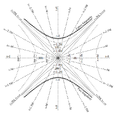
Figure 1: The maximal analytical extension of the Schwarzschild metric for the parameter $E$ generic obeying $E>1$ in the plane $({\mathcal{t}}^{\prime},\tau^{\prime})$ is shown in a diagram with two different descriptions, (a) and (b). In (a) typical values for lines of constant ${\mathcal{t}}^{\prime}$ and constant $\tau^{\prime}$ are displayed. In (b) typical values for lines of constant $t$ and constant $r$ are displayed. The diagram, both in (a) and in (b), represents a a spacetime with a wormhole, not shown, that forms out of a singularity in the white hole region, i.e., region IV, and finishes at the black hole region and its singularity, i.e., region II, connecting the two separated asymptotically flat spacetimes, regions I and III.

It is also worth discussing the normals to the ${\mathcal{t}}^{\prime}={\rm constant}$ and $\tau^{\prime}={\rm constant}$ hypersurfaces. From Eq. (13) one finds that the covariant metric has components $g_{{\mathcal{t}^{\prime}}{\mathcal{t}^{\prime}}}=\frac{4}{M^{2}}\left(\frac{\left(2E^{2}-1+\frac{2M}{r}+2E\sqrt{E^{2}-1+\frac{2M}{r}}\right)^{2}}{E^{2}-1+\frac{2M}{r}}\right)\exp{\left(-\frac{r}{ME}\sqrt{E^{2}-1+\frac{2M}{r}}\right)}\times\allowbreak\times\left(\frac{\frac{M}{r}}{E^{2}-1+\frac{M}{r}+\sqrt{E^{2}-1}\sqrt{E^{2}-1+\frac{2M}{r}}}\right)^{\frac{2E^{2}-1}{E\sqrt{E^{2}-1}}}\tau^{\prime 2}$, $g_{\tau^{\prime}\tau^{\prime}}=\frac{4}{M^{2}}\left(\frac{\left(2E^{2}-1+\frac{2M}{r}+2E\sqrt{E^{2}-1+\frac{2M}{r}}\right)^{2}}{E^{2}-1+\frac{2M}{r}}\right)\exp{\left(-\frac{r}{ME}\sqrt{E^{2}-1+\frac{2M}{r}}\right)}\times\allowbreak\times\left(\frac{\frac{M}{r}}{E^{2}-1+\frac{M}{r}+\sqrt{E^{2}-1}\sqrt{E^{2}-1+\frac{2M}{r}}}\right)^{\frac{2E^{2}-1}{E\sqrt{E^{2}-1}}}{\mathcal{t}}^{\prime 2}$, $g_{{\mathcal{t}^{\prime}}\tau^{\prime}}=g_{\tau^{\prime}{\mathcal{t}^{\prime}}}=-4\left(\frac{2E^{2}-1+\frac{2M}{r}+2E\sqrt{E^{2}-1+\frac{2M}{r}}}{E^{2}-1+\frac{2M}{r}}\right)\left(2E^{2}-1+\frac{2M}{r}\right)\times\allowbreak\times\exp{\left(-\frac{r}{2ME}\sqrt{E^{2}-1+\frac{2M}{r}}\right)}\left(\frac{\frac{M}{r}}{E^{2}-1+\frac{M}{r}+\sqrt{E^{2}-1}\sqrt{E^{2}-1+\frac{2M}{r}}}\right)^{\frac{2E^{2}-1}{2E\sqrt{E^{2}-1}}}$, $g_{\theta\theta}=r^{2}$, $g_{\phi\phi}=r^{2}\sin^{2}{\theta}$. The contravariant components of the metric can be calculated to be $g^{{\mathcal{t}}^{\prime}{\mathcal{t}}^{\prime}}=-\frac{{\mathcal{t}}^{\prime 2}}{16M^{2}E^{2}}$, $g^{{\tau}^{\prime}{\tau}^{\prime}}=-\frac{\tau^{\prime 2}}{16M^{2}E^{2}}$, $g^{{\mathcal{t}}^{\prime}\tau^{\prime}}=g^{\tau^{\prime}{\mathcal{t}}^{\prime}}=\allowbreak=-\frac{1}{16E^{2}}\frac{1}{2E^{2}-1+\frac{2M}{r}+2E\sqrt{E^{2}-1+\frac{2M}{r}}}\left(2E^{2}-1+\frac{2M}{r}\right)\left[\frac{r}{M}\left(E^{2}-1+\frac{M}{r}+\sqrt{E^{2}-1}\sqrt{E^{2}-1+\frac{2M}{r}}\right)\right]^{\frac{2E^{2}-1}{2E\sqrt{E^{2}-1}}}\times\\ \times\exp{\left(\frac{r}{2ME}\sqrt{E^{2}-1+\frac{2M}{r}}\right)}$, $g^{\theta\theta}=\frac{1}{r^{2}}$, $g^{\phi\phi}=\frac{1}{r^{2}\sin^{2}{\theta}}$. The normals $n_{a}$ to the ${\mathcal{t}}^{\prime}={\rm constant}$ and $\tau^{\prime}={\rm constant}$ hypersurfaces are ${n^{\mathcal{t}^{\prime}}}_{a}=(1,0,0,0)$ and ${n^{\tau^{\prime}}}_{a}=(0,1,0,0)$, respectively, where the superscripts ${\mathcal{t}^{\prime}}$ and $\tau^{\prime}$ in this context are not indices, they simply label the respective normal. Their contravariant components are, respectively, $n^{{\mathcal{t}^{\prime}}\hskip 0.1424pta}=(g^{{\mathcal{t}}^{\prime}{\mathcal{t}}^{\prime}},g^{{\mathcal{t}}^{\prime}\tau^{\prime}},0,0)$ and $n^{\tau^{\prime}\hskip 0.1424pta}=(g^{\tau^{\prime}{\mathcal{t}}^{\prime}},g^{\tau^{\prime}\tau^{\prime}},0,0)$, awkward writing them explicitly due to the long expression for $g^{{\mathcal{t}}^{\prime}\tau^{\prime}}$. The norms are then ${n^{\mathcal{t}^{\prime}}}_{a}n^{{\mathcal{t}^{\prime}}\hskip 0.1424pta}=-\frac{{\mathcal{t}}^{\prime 2}}{16M^{2}E^{2}}$ and ${n^{\tau^{\prime}}}_{a}n^{{\tau^{\prime}}\hskip 0.1424pta}=-\frac{\tau^{\prime 2}}{16M^{2}E^{2}}$, respectively. Thus, clearly, the normals to the ${\mathcal{t}^{\prime}}={\rm constant}$ and $\tau^{\prime}={\rm constant}$ hypersurfaces are timelike, and so ${\mathcal{t}}^{\prime}$ and $\tau^{\prime}$ are timelike coordinates, and the corresponding hypersurfaces are spacelike, only in a measure zero are they null, when ${\mathcal{t}}^{\prime}=0$ and $\tau^{\prime}=0$, respectively.

IV Maximal analytic extension for $E=1$ as the lower limit of $E>1$

To build the maximal analytic extension for $E=1$, we take the $E\to 1$ limit from the $E>1$ case. Using $\ln\Big{[}\left(2\sqrt{E^{2}-1}\sqrt{\frac{r}{2M}}\right)+1\Big{]}=2\sqrt{E^{2}-1}\sqrt{\frac{r}{2M}}$ in this limit, we find that the coordinates ${\mathcal{t}}$ and $\tau$ of Eqs. (7) and (8) become

$${\mathcal{t}} =t-4M\sqrt{\frac{r}{2M}}+2M\ln{\left|\frac{\sqrt{\frac{r}{2M}}+1}{\sqrt{\frac{r}{2M}}-1}\right|}\,,$$ (15)

$$\tau =t+4M\sqrt{\frac{r}{2M}}-2M\ln{\left|\frac{\sqrt{\frac{r}{2M}}+1}{\sqrt{\frac{r}{2M}}-1}\right|}\,.$$ (16)

The line element given in Eq. (9) is then in this $E=1$ limit given by

$$\mathrm{d}s^{2}=-\frac{1}{4}\frac{\left(1-\frac{2M}{r}\right)}{\frac{2M}{r}}\left[-\left(1-\frac{2M}{r}\right)(\mathrm{d}{\mathcal{t}}^{2}+\mathrm{d}\tau^{2})+2\left(1+\frac{2M}{r}\right)\mathrm{d}{\mathcal{t}}\,\mathrm{d}\tau\right]+r^{2}(\mathrm{d}\theta^{2}+\sin^{2}{\theta}\,\mathrm{d}\phi^{2})\,,$$ (17)

with $r=r({\mathcal{t}},\tau)$ being obtained via Eq. (III) in the $E=1$ limit, or through Eqs. (15) and (16), i.e.,

$$4M\sqrt{\dfrac{r}{2M}}-2M\ln{\left|\frac{\sqrt{\frac{r}{2M}}+1}{\sqrt{\frac{r}{2M}}-1}\right|}=\frac{1}{2}\left(-{\mathcal{t}}+\tau\right)\,.$$ (18)

Again, as in Eq. (9), the line element given in Eq. (17) is still degenerate at $r=2M$. So, to extend it past $r=2M$ we again make use of maximal extended coordinates, ${\mathcal{t}}^{\prime}$ and $\tau^{\prime}$, defined as $\frac{{\mathcal{t}}^{\prime}}{M}=-\exp{\left(-\frac{{\mathcal{t}}}{4M}\right)}$ and $\frac{\tau^{\prime}}{M}=\exp{\left(\frac{\tau}{4M}\right)}$, which by either taking directly the limit $E=1$ in Eqs. (11) and (12), respectively, or using Eqs. (15) and (16), yields for $r>2M$,

$$\frac{{\mathcal{t}}^{\prime}}{M} =-\exp{\left(-\frac{{\mathcal{t}}}{4M}\right)}\,,\quad{\rm i.e.,}\quad\frac{{\mathcal{t}}^{\prime}}{M}=-\sqrt{\frac{\sqrt{\frac{r}{2M}}-1}{\sqrt{\frac{r}{2M}}+1}}\exp{\left(-\frac{t}{4M}+\sqrt{\frac{r}{2M}}\right)}\,,$$ (19)

$$\frac{\tau^{\prime}}{M} =\quad\exp{\left(\;\frac{\tau}{4M}\right)}\,,\;\;\,\quad{\rm i.e.,}\quad\frac{\tau^{\prime}}{M}=\quad\sqrt{\frac{\sqrt{\frac{r}{2M}}-1}{\sqrt{\frac{r}{2M}}+1}}\exp{\left(\;\frac{t}{4M}+\sqrt{\frac{r}{2M}}\right)}\,,$$ (20)

respectively. Through the $E=1$ limit of Eq. (13), or putting ${\mathcal{t}}^{\prime}$ and $\tau^{\prime}$ given in Eqs. (19) and (20), respectively, into the line element Eq. (17), one finds that the new $E=1$ line element in coordinates $({\mathcal{t}}^{\prime},\tau^{\prime},\theta,\phi)$ is given by

$$\begin{split}\mathrm{d}s^{2}=&-4\frac{\left(1+\sqrt{\frac{2M}{r}}\right)^{2}}{\frac{2M}{r}}\exp{\left(-2\sqrt{\frac{r}{2M}}\right)}\left[-\frac{1}{M^{2}}\left(1+\sqrt{\frac{2M}{r}}\right)^{2}\exp{\left(-2\sqrt{\frac{r}{2M}}\right)}(\tau^{\prime 2}\,\mathrm{d}{\mathcal{t}}^{\prime 2}+{\mathcal{t}}^{\prime 2}\,\mathrm{d}\tau^{\prime 2})+\right.\\ &\left.+2\left(1+\frac{2M}{r}\right)\mathrm{d}{\mathcal{t}}^{\prime}\,\mathrm{d}\tau^{\prime}\right]+r^{2}(\mathrm{d}\theta^{2}+\sin^{2}{\theta}\,\mathrm{d}\phi^{2})\,,\end{split}$$ (21)

with $r=r({\mathcal{t}}^{\prime},\tau^{\prime})$ given implicitly, see Eq. (14) in the $E=1$ limit, or directly through Eqs. (19) and (20), by

$$\frac{\sqrt{\frac{r}{2M}}-1}{\sqrt{\frac{r}{2M}}+1}\exp{\left(2\sqrt{\frac{r}{2M}}\right)}=-\frac{{\mathcal{t}}^{\prime}}{M}\frac{\tau^{\prime}}{M}\,.$$ (22)

All of this is done so that ${\mathcal{t}}^{\prime}$ and $\tau^{\prime}$ have ranges $-\infty<{\mathcal{t}}^{\prime}<\infty$ and $-\infty<\tau^{\prime}<\infty$, which Eqs. (21) and (22) permit. To obtain Eqs. (21) and (22) directly from the $E\to 1$ limit of Eqs. (13) and (14), respectively, see the Appendix. Several properties are again worth mentioning.

In terms of the coordinates $({\mathcal{t}},\tau)$, or $(t,r)$, the coordinate transformations that yield the maximal extended coordinates $({\mathcal{t}}^{\prime},\tau^{\prime})$ with infinite ranges have to be broadened, resulting in the existence of four regions, regions I, II, III, and IV. Region I is the region where the transformations Eqs. (19) and (20) hold, i.e., it is a region with ${\mathcal{t}}^{\prime}\leq 0$ and $\tau^{\prime}\geq 0$. It is a region with $r\geq 2M$ and $-\infty<t<\infty$. Of course, in this region Eqs. (21) and (22) hold. Region II, a region for which $r\leq 2M$, gets a different set of coordinate transformations. In this $r\leq 2M$ region, due to the moduli appearing in Eqs. (19) and (20) and the change of sign in Eq. (17), one defines instead ${\mathcal{t}}^{\prime}$ as $\frac{{\mathcal{t}}^{\prime}}{M}=+\exp{\left(-\frac{{\mathcal{t}}}{4M}\right)}=\\ =+\sqrt{\frac{1-\sqrt{\frac{r}{2M}}}{1+\sqrt{\frac{r}{2M}}}}\exp{\left(-\frac{t}{4M}+\sqrt{\frac{r}{2M}}\right)}$ and $\tau^{\prime}$ as $\frac{\tau^{\prime}}{M}=\exp{\left(\frac{\tau}{4M}\right)}=\sqrt{\frac{1-\sqrt{\frac{r}{2M}}}{1+\sqrt{\frac{r}{2M}}}}\exp{\left(\;\frac{t}{4M}+\sqrt{\frac{r}{2M}}\right)}$. These transformations are valid for ${\mathcal{t}}^{\prime}\geq 0$ and $\tau^{\prime}\geq 0$. It is a region with $r\leq 2M$ and $-\infty<t<\infty$. Note that the coordinate transformations in this region give $\frac{1-\sqrt{\frac{r}{2M}}}{1+\sqrt{\frac{r}{2M}}}\exp{\left(2\sqrt{\frac{r}{2M}}\right)}=\frac{{\mathcal{t}}^{\prime}}{M}\frac{\tau^{\prime}}{M}$ But all this has been automatically incorporated into Eqs. (21) and (22) so there is no further concern on that. Region III is another $r\geq 2M$ region. Now one defines ${\mathcal{t}}^{\prime}$ as $\frac{{\mathcal{t}}^{\prime}}{M}=\exp{\left(-\frac{{\mathcal{t}}}{4M}\right)}=\sqrt{\frac{\sqrt{\frac{r}{2M}}-1}{\sqrt{\frac{r}{2M}}+1}}\exp{\left(-\frac{t}{4M}+\sqrt{\frac{r}{2M}}\right)}$ and $\tau^{\prime}$ as $\frac{\tau^{\prime}}{M}=-\exp{\left(\frac{\tau}{4M}\right)}=-\sqrt{\frac{\sqrt{\frac{r}{2M}}-1}{\sqrt{\frac{r}{2M}}-1}}\exp{\left(\;\frac{t}{4M}+\sqrt{\frac{r}{2M}}\right)}$. These transformations are valid for the region with ${\mathcal{t}}^{\prime}\geq 0$ and $\tau^{\prime}\leq 0$. It is a region with $r\geq 2M$ and $-\infty<t<\infty$. Note that the coordinate transformations in this region give $\frac{\sqrt{\frac{r}{2M}}-1}{\sqrt{\frac{r}{2M}}+1}\exp{\left(2\sqrt{\frac{r}{2M}}\right)}=-\frac{{\mathcal{t}}^{\prime}}{M}\frac{\tau^{\prime}}{M}$ But all this has been automatically incorporated into Eqs. (21) and (22) so again there is no further concern on that. Region IV is another region with $r\leq 2M$. Now, one defines ${\mathcal{t}}^{\prime}$ as $\frac{{\mathcal{t}}^{\prime}}{M}=-\exp{\left(-\frac{{\mathcal{t}}}{4M}\right)}=-\sqrt{\frac{1-\sqrt{\frac{r}{2M}}}{1+\sqrt{\frac{r}{2M}}}}\exp{\left(-\frac{t}{4M}+\sqrt{\frac{r}{2M}}\right)}$ and $\tau^{\prime}$ as $\frac{\tau^{\prime}}{M}=-\exp{\left(\frac{\tau}{4M}\right)}=-\sqrt{\frac{1-\sqrt{\frac{r}{2M}}}{1+\sqrt{\frac{r}{2M}}}}\exp{\left(\;\frac{t}{4M}+\sqrt{\frac{r}{2M}}\right)}$. These transformations are valid for the region with ${\mathcal{t}}^{\prime}\leq 0$ and $\tau^{\prime}\leq 0$. It is a region with $r\leq 2M$ and $-\infty<t<\infty$. Note that the coordinate transformations in this region give $\frac{1-\sqrt{\frac{r}{2M}}}{1+\sqrt{\frac{r}{2M}}}\exp{\left(2\sqrt{\frac{r}{2M}}\right)}=\frac{{\mathcal{t}}^{\prime}}{M}\frac{\tau^{\prime}}{M}$. But all this has been automatically incorporated into Eqs. (21) and (22) so once again there is no further concern on that.

Furthermore, from Eq. (22) we see that the event horizon at $r=2M$ has two solutions, ${\mathcal{t}}^{\prime}=0$ and $\tau^{\prime}=0$ which are null surfaces represented by straight lines. The true curvature singularity at $r=0$ has two solutions $\frac{{\mathcal{t}}^{\prime}}{M}\frac{\tau^{\prime}}{M}=1$, i.e., two spacelike hyperbolae. Implicit in the construction, there is a wormhole, or Einstein-Rosen bridge, topology, with its throat expanding and contracting. The dynamic wormhole is non traversable, but it spatially connects region I to region III through regions II and IV. Regions I and III are two asympotically flat regions causally separated, region II is the black hole region, and region IV is the white hole region of the spacetime.

Eqs. (21) and (22) together with the corresponding interpretation give the maximal extension of the Schwarzschild metric for $E=1$, in the coordinates $({\mathcal{t}}^{\prime},\tau^{\prime},\theta,\phi)$. The two-dimensional part $({\mathcal{t}}^{\prime},\tau^{\prime})$ of the coordinate system $({\mathcal{t}}^{\prime},\tau^{\prime},\theta,\phi)$ is shown in Figure 2, both for lines of constant ${\mathcal{t}}^{\prime}$ and constant $\tau^{\prime}$ in part (a) of the figure, and for lines of constant $t$ and constant $r$ in part (b) of the figure, conjointly with the labeling of regions I, II, III, IV, needed to cover it.

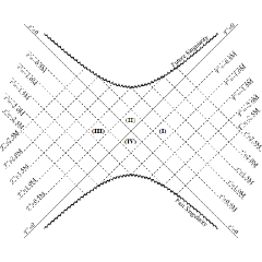
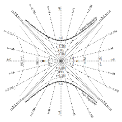
Figure 2: The maximal analytical extension of the Schwarzschild metric for the parameter $E=1$ in the plane $({\mathcal{t}}^{\prime},\tau^{\prime})$ is shown in a diagram with two different descriptions, (a) and (b). In (a) typical values for lines of constant ${\mathcal{t}}^{\prime}$ and constant $\tau^{\prime}$ are displayed. In (b) typical values for lines of constant $t$ and constant $r$ are displayed. The diagram, both in (a) and in (b), represents a a spacetime with a wormhole, not shown, that forms out of a singularity in the white hole region, i.e., region IV, and finishes at the black hole region and its singularity, i.e., region II, connecting the two separated asymptotically flat spacetimes, regions I and III. The $E=1$ diagram is very similar to the $E>1$ generic case diagram, see Figure 1, as it is expected for a maximal extension of the Schwarzschild spacetime, in particular for those extensions within the same family.

It is also worth discussing the normals to the ${\mathcal{t}}^{\prime}={\rm constant}$ and $\tau^{\prime}={\rm constant}$ hypersurfaces. From Eq. (21) one finds that the metric has covariant components $g_{{\mathcal{t}^{\prime}}{\mathcal{t}^{\prime}}}=\frac{4}{M^{2}}\frac{\left(1+\sqrt{\frac{2M}{r}}\right)^{4}}{\frac{2M}{r}}\exp{\left(-4\sqrt{\frac{r}{2M}}\right)}\tau^{\prime 2}$, $g_{\tau^{\prime}\tau^{\prime}}=\frac{4}{M^{2}}\frac{\left(1+\sqrt{\frac{2M}{r}}\right)^{4}}{\frac{2M}{r}}\times\\ \times\exp{\left(-4\sqrt{\frac{r}{2M}}\right)}{\mathcal{t}}^{\prime 2}$, $g_{{\mathcal{t}^{\prime}}\tau^{\prime}}=g_{\tau^{\prime}{\mathcal{t}^{\prime}}}=-4\frac{\left(1+\sqrt{\frac{2M}{r}}\right)^{2}}{\frac{2M}{r}}\left(1+\frac{2M}{r}\right)\exp{\left(-2\sqrt{\frac{r}{2M}}\right)}$, $g_{\theta\theta}=r^{2}$, $g_{\phi\phi}=r^{2}\sin^{2}{\theta}$. The contravariant components of the metric can be calculated to be $g^{{\mathcal{t}}^{\prime}{\mathcal{t}}^{\prime}}=-\frac{{\mathcal{t}}^{\prime 2}}{16M^{2}}$, $g^{{\tau}^{\prime}{\tau}^{\prime}}=-\frac{\tau^{\prime 2}}{16M^{2}}$, $g^{{\mathcal{t}}^{\prime}\tau^{\prime}}=g^{\tau^{\prime}{\mathcal{t}}^{\prime}}=-\frac{1}{16}\frac{1+\frac{2M}{r}}{\left(1+\sqrt{\frac{2M}{r}}\right)^{2}}\times\\ \times\exp{\left(2\sqrt{\frac{r}{2M}}\right)}$, $g^{\theta\theta}=\frac{1}{r^{2}}$, $g^{\phi\phi}=\frac{1}{r^{2}\sin^{2}{\theta}}$. The normals $n_{a}$ to the ${\mathcal{t}}^{\prime}={\rm constant}$ and $\tau^{\prime}={\rm constant}$ hypersurfaces are ${n^{\mathcal{t}^{\prime}}}_{a}=(1,0,0,0)$ and ${n^{\tau^{\prime}}}_{a}=(0,1,0,0)$, respectively, where the superscripts ${\mathcal{t}^{\prime}}$ and $\tau^{\prime}$ in this context are not indices, they simply label the respective normal. Their contravariant components are $n^{{\mathcal{t}^{\prime}}\hskip 0.1424pta}=(g^{{\mathcal{t}}^{\prime}{\mathcal{t}}^{\prime}},g^{{\mathcal{t}}^{\prime}\tau^{\prime}},0,0)=\allowbreak{=(-\frac{{\mathcal{t}}^{\prime 2}}{16M^{2}},-\frac{1}{16}\frac{1+\frac{2M}{r}}{\left(1+\sqrt{\frac{2M}{r}}\right)^{2}}\exp{\left(2\sqrt{\frac{r}{2M}}\right)}},0,0)$ and $n^{\tau^{\prime}\hskip 0.1424pta}=(g^{\tau^{\prime}{\mathcal{t}}^{\prime}},g^{\tau^{\prime}\tau^{\prime}},0,0)=(-\frac{1}{16}\frac{1+\frac{2M}{r}}{\left(1+\sqrt{\frac{2M}{r}}\right)^{2}}\exp{\left(2\sqrt{\frac{r}{2M}}\right)},-\frac{\tau^{\prime 2}}{16M^{2}},0,0)$, respectively. The norms are then ${n^{\mathcal{t}^{\prime}}}_{a}n^{{\mathcal{t}^{\prime}}\hskip 0.1424pta}=-\frac{{\mathcal{t}}^{\prime 2}}{16M^{2}}$ and ${n^{\tau^{\prime}}}_{a}n^{{\tau^{\prime}}\hskip 0.1424pta}=-\frac{\tau^{\prime 2}}{16M^{2}}$, respectively. Thus, clearly, the normals to the ${\mathcal{t}^{\prime}}={\rm constant}$ and $\tau^{\prime}={\rm constant}$ hypersurfaces are timelike, and so ${\mathcal{t}}^{\prime}$ and $\tau^{\prime}$ are timelike coordinates, and the corresponding hypersurfaces are spacelike, only in a measure zero are they null, when ${\mathcal{t}}^{\prime}=0$ and $\tau^{\prime}=0$, respectively. The metric components and the normals can also be found from the $E>1$ case in the $E=1$ limit.

V Maximal analytic extension for $E=\infty$ as the upper limit of $E>1$: The Kruskal-Szekeres maximal extension of the Schwarzschild metric

To build the maximal analytic extension for $E=\infty$, we take the $E\to\infty$ limit from the $E>1$ generic case. We will see that this limit is the Kruskal-Szekeres maximal analytic extension. Taking a redefinition of the coordinates $\tau$ and ${\mathcal{t}}$ of Eqs. (7) and (8) to coordinates $u$ and $v$, respectively, we find that these become

$$u \equiv\lim_{E\to\infty}\frac{{\mathcal{t}}}{E}\,,\quad{\rm i.e.,}\quad\quad u=t-r-2M\ln{\left|\frac{r}{2M}-1\right|}\,,$$ (23)

$$v \equiv\lim_{E\to\infty}\frac{\tau}{E}\,,\quad{\rm i.e.,}\quad\quad v=t+r+2M\ln{\left|\frac{r}{2M}-1\right|}\,.$$ (24)

The line element given in Eq. (9) is then in this limit

$$\mathrm{d}s^{2}=-\left(1-\frac{2M}{r}\right)dudv+r^{2}(\mathrm{d}\theta^{2}+\sin^{2}{\theta}\,\mathrm{d}\phi^{2})\,.$$ (25)

with $r=r(u,v)$ being obtained directly via Eq. (III) in the $E\to\infty$ limit, or through Eqs. (23) and (24), i.e.,

$$r+2M\ln{\left|\frac{r}{2M}-1\right|}=\frac{1}{2}\left(-u+v\right)\,.$$ (26)

Again, the line element given in Eq. (25) is still degenerate at $r=2M$. So, to extend it past $r=2M$, we make use of the maximal extended timelike coordinates ${\mathcal{t}}^{\prime}$ and $\tau^{\prime}$ defined through $\frac{{\mathcal{t}}^{\prime}}{M}=-\exp{\left(-\frac{{\mathcal{t}}}{4ME}\right)}$ and $\frac{\tau^{\prime}}{M}=\exp{\left(\;\frac{\tau}{4ME}\right)}$, which in this limit $E\to\infty$ are redefined to maximal extended coordinates, $u^{\prime}$ and $v^{\prime}$, respectively, obtained directly via Eqs. (11) and (12) in the $E\to\infty$ limit, or using Eqs. (23) and (24), to find

$$u^{\prime} =\lim_{E\to\infty}{\mathcal{t}^{\prime}}\,,\quad{\rm i.e.,}\quad\quad\frac{u^{\prime}}{M}=-\exp{\left(-\frac{u}{4M}\right)}\,,\quad\quad{\rm i.e.,}\quad\quad\frac{u^{\prime}}{M}=-\sqrt{\frac{r}{2M}-1}\,\exp{\left(-\frac{t}{4M}+\frac{r}{4M}\right)}\,,$$ (27)

$$v^{\prime} =\lim_{E\to\infty}\tau^{\prime}\,,\quad{\rm i.e.,}\quad\quad\frac{v^{\prime}}{M}=\quad\exp{\left(\frac{v}{4M}\right)}\,,\quad\quad\;\;\;{\rm i.e.,}\quad\quad\frac{v^{\prime}}{M}=\quad\sqrt{\frac{r}{2M}-1}\,\exp{\left(\frac{t}{4M}+\frac{r}{4M}\right)}\,.$$ (28)

Then, the line element of (13) in the $E\to\infty$ limit, or through Eq. (25) together with Eqs. (27) and (28), yields the new line element

$$\mathrm{d}s^{2}=-\frac{32M}{r}\exp{\left(-\frac{r}{2M}\right)}\mathrm{d}u^{\prime}\,\mathrm{d}v^{\prime}+r^{2}(\mathrm{d}\theta^{2}+\sin^{2}{\theta}\,\mathrm{d}\phi^{2})\,,$$ (29)

with $r=r(u^{\prime},v^{\prime})$ given implicitly, see Eq. (14) in the $E\to\infty$ limit, or directly through Eqs. (27) and (28), by

$$\left(\frac{r}{2M}-1\right)\exp{\left(\frac{r}{2M}\right)}=-\frac{u^{\prime}}{M}\frac{v^{\prime}}{M}\,.$$ (30)

All of this is done so that $u^{\prime}$ and $v^{\prime}$ have ranges $-\infty<u^{\prime}<\infty$ and $-\infty<v^{\prime}<\infty$, which Eqs. (29) and (30) permit. To obtain Eqs. (29) and (30) directly from the $E\to\infty$ limit of Eqs. (13) and (14), respectively, see the Appendix. Several properties are worth mentioning.

In terms of the coordinates $(u,v)$, or $(t,r)$, the coordinate transformations that yield the maximal extended null coordinates $(u^{\prime},v^{\prime})$ with infinite ranges have to be broadened, resulting in the existence of four regions, regions I, II, III, and IV. Region I is the region where the transformations Eqs. (27) and (28) hold, i.e., it is a region with $u^{\prime}\leq 0$ and $v^{\prime}\geq 0$, or a region with $r\geq 2M$ and $-\infty<t<\infty$. Region II, a region for which $r\leq 2M$, gets a different set of coordinate transformations. In this region $r\leq 2M$, due to the moduli appearing in Eqs. (23) and (24) and the change of sign in Eq. (25), one defines instead $u^{\prime}$ as $\frac{u^{\prime}}{M}=+\exp{\left(-\frac{u}{4M}\right)}=\sqrt{1-\frac{r}{2M}}\,\exp{\left(-\frac{t}{4M}+\frac{r}{4M}\right)}$ and $v^{\prime}$ as $\frac{v^{\prime}}{M}=\exp{\left(\frac{v}{4M}\right)}=\sqrt{1-\frac{r}{2M}}\,\exp{\left(\frac{t}{4M}+\frac{r}{4M}\right)}$. These transformations are valid for the region with $u^{\prime}\geq 0$ and $v^{\prime}\geq 0$, or the region with $r\leq 2M$ and $-\infty<t<\infty$. Note that the coordinate transformations in this region give $\left(1-\frac{r}{2M}\right)\exp{\left(\frac{r}{2M}\right)}=\frac{u^{\prime}}{M}\frac{v^{\prime}}{M}$. But this is automatically incorporated into Eq. (30), so there is no further concern on that. Region III is another $r\geq 2M$ region. Now one defines $\frac{u^{\prime}}{M}=\exp{\left(-\frac{u}{4M}\right)}=\sqrt{\frac{r}{2M}-1}\,\exp{\left(-\frac{t}{4M}+\frac{r}{4M}\right)}$ and $v^{\prime}$ as $\frac{v^{\prime}}{M}=-\exp{\left(\frac{v}{4M}\right)}=-\sqrt{\frac{r}{2M}-1}\,\exp{\left(\frac{t}{4M}+\frac{r}{4M}\right)}$. These transformations are valid for the region with $u^{\prime}\geq 0$ and $v^{\prime}\leq 0$, or the region with $r\geq 2M$ and $-\infty<t<\infty$. Note that the coordinate transformations in this region give $\left(\frac{r}{2M}-1\right)\exp{\left(\frac{r}{2M}\right)}=-\frac{u^{\prime}}{M}\frac{v^{\prime}}{M}$. But this is automatically incorporated into Eq. (30), so again there is no further concern on that. Region IV is another region with $r\leq 2M$. Now, one defines $u^{\prime}$ as $\frac{u^{\prime}}{M}=-\exp{\left(-\frac{u}{4M}\right)}=\allowbreak=-\sqrt{1-\frac{r}{2M}}\,\exp{\left(-\frac{t}{4M}+\frac{r}{4M}\right)}$ and $v^{\prime}$ as $\frac{v^{\prime}}{M}=-\exp{\left(\frac{v}{4M}\right)}=-\sqrt{1-\frac{r}{2M}}\,\exp{\left(\frac{t}{4M}+\frac{r}{4M}\right)}$. These transformations are valid for the region with $u^{\prime}\leq 0$ and $v^{\prime}\leq 0$, or the region with $r\leq 2M$ and $-\infty<t<\infty$. The coordinate transformations in this region give as well $\left(1-\frac{r}{2M}\right)\exp{\left(\frac{r}{2M}\right)}=\frac{u^{\prime}}{M}\frac{v^{\prime}}{M}$. But this is automatically incorporated into Eq. (30), so once again there is no further concern on that.

Furthermore, from Eq. (30) we see that the event horizon at $r=2M$ has two solutions, $u^{\prime}=0$ and $v^{\prime}=0$ which are null surfaces represented by straight lines. The true curvature singularity at $r=0$ has two solutions $\frac{u^{\prime}}{M}\frac{v^{\prime}}{M}=1$, i.e., two spacelike hyperbolae. Implicit in the construction, there is a wormhole, or Einstein-Rosen bridge, topology, with its throat expanding and contracting. The dynamic wormhole is non traversable, but it spatially connects region I to region III through regions II and IV. Regions I and III are two asympotically flat regions causally separated, region II is the black hole region, and region IV is the white hole region of the spacetime.

Eqs. (29) and (30) together with the corresponding interpretation give the maximal extension of the Schwarzschild metric for $E=\infty$, taken as the limit of $E>1$, in the coordinates $(u^{\prime},v^{\prime},\theta,\phi)$. Of course, this the Kruskal-Szekeres maximal analytical extension, now seen as the $E=\infty$ member of the family of extensions of $E>1$. Recalling that $u^{\prime}={\mathcal{t}}^{\prime}|_{E=\infty}$ and $v^{\prime}=\tau^{\prime}|_{E=\infty}$, we see that the two timelike congruences that specify the two analytically extended time coordinates $\mathcal{t}^{\prime}$ and $\tau^{\prime}$ that yield the maximal extension for $E>1$ turned into the two analytically extended null retarded and advanced congruences $u^{\prime}$ and $v^{\prime}$ of the Kruskal-Szekeres maximal extension. The two-dimensional part $(u^{\prime},v^{\prime})$ of the coordinate system $(u^{\prime},v^{\prime},\theta,\phi)$ is shown in Figure 3 , both for lines of constant $u^{\prime}$ and constant $v^{\prime}$ in part (a) of the figure, and for lines of constant $t$ and constant $r$ in part (b) of the figure, conjointly with the labeling of regions I, II, III, IV, needed to cover it.

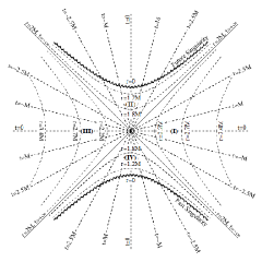
Figure 3: The maximal analytical extension of the Schwarzschild metric for the parameter $E=\infty$, i.e., the Kruskal-Szekeres maximal extension, in the plane $(u^{\prime},v^{\prime})$ is shown in a diagram with two different descriptions, (a) and (b). In (a) typical values for lines of constant $u^{\prime}$ and constant $v^{\prime}$ are displayed. In (b) typical values for lines of constant $t$ and constant $r$ are displayed. The diagram, both in (a) and in (b), represents a spacetime with a wormhole, not shown, that forms out of a singularity in the white hole region, i.e., region IV, and finishes at the black hole region and its singularity, i.e., region II, connecting the two separated asymptotically flat spacetimes, regions I and III. The $E=\infty$ diagram, i.e., the Kruskal-Szekeres diagram, is very similar to the $E>1$ generic case diagram, see Figure 1, as it is expected for a maximal extension of the Schwarzschild spacetime, in particular for those extensions within the same family.

It is also worth discussing the normals to the $u^{\prime}={\rm constant}$ and $v^{\prime}={\rm constant}$ hypersurfaces. For that, we see that from Eq. (13) in the limit $E\to\infty$, or directly from Eq. (29), one finds that the metric has covariant components $g_{u^{\prime}u^{\prime}}=0$, $g_{v^{\prime}v^{\prime}}=0$, $g_{u^{\prime}v^{\prime}}=g_{v^{\prime}u^{\prime}}=-\frac{16M}{r}\exp{\left(-{\frac{r}{2M}}\right)}$, $g_{\theta\theta}=r^{2}$, $g_{\phi\phi}=r^{2}\sin^{2}{\theta}$. The contravariant components of the metric can be calculated to be $g^{u^{\prime}u^{\prime}}=0$, $g^{v^{\prime}v^{\prime}}=0$, $g^{u^{\prime}v^{\prime}}=g^{v^{\prime}u^{\prime}}=-\frac{r}{16M}\exp{\left(\frac{r}{2M}\right)}$, $g^{\theta\theta}=\frac{1}{r^{2}}$, $g^{\phi\phi}=\frac{1}{r^{2}\sin^{2}{\theta}}$. The normals $n_{a}$ to the $u^{\prime}={\rm constant}$ and $v^{\prime}={\rm constant}$ hypersurfaces are ${n^{u^{\prime}}}_{a}=(1,0,0,0)$ and ${n^{v^{\prime}}}_{a}=(0,1,0,0)$, respectively, where the superscripts $u^{\prime}$ and $v^{\prime}$ in this context are not indices, they simply label the respective normal. Their contravariant components are $n^{{u^{\prime}}\hskip 0.1424pta}=(g^{u^{\prime}u^{\prime}},g^{u^{\prime}v^{\prime}},0,0)=(0,-\frac{r}{16M}\exp{\left(\frac{r}{2M}\right)},0,0)$ and $n^{{v^{\prime}}\hskip 0.1424pta}=(g^{v^{\prime}u^{\prime}},g^{v^{\prime}v^{\prime}},0,0)=(-\frac{r}{16M}\exp{\left(\frac{r}{2M}\right)},0,0,0)$. The norms are then ${n^{u^{\prime}}}_{a}n^{{u^{\prime}}\hskip 0.1424pta}=0$ and ${n^{v^{\prime}}}_{a}n^{{v^{\prime}}\hskip 0.1424pta}=0$, respectively. Thus, clearly, the normals to the $u^{\prime}={\rm constant}$ and $v^{\prime}={\rm constant}$ hypersurfaces are null, and so $u^{\prime}$ and $v^{\prime}$ are null coordinates, and the corresponding hypersurfaces are null as well.

VI Causal diagrams from $E=1$ to $E=\infty$

In this unified account that carries maximal extensions of the Schwarzschild metric along the parameter $E$, it is of interest to trace the radial null geodesics for several values of the parameter $E$ itself, $1\leq E\leq\infty$, in the plane characterized by the $({\mathcal{t}}^{\prime},\tau^{\prime})$ coordinates. Null geodesics have $ds^{2}=0$ along them, and if they are radial then also $d\theta=0$ and $d\phi=0$. Using the line element given in Eq. (13) together with Eq. (14), we can then trace the radial null geodesics, and with it the causal structure for each $E$, in the corresponding maximally analytic extended diagram. Figures 4, 5, 6, and 7 are the maximal extended causal diagrams for $E=1.0$, $E=1.1$, $E=1.5$, and $E=\infty$, respectively. In the $E=1$ case one can take the null geodesics directly from Eqs. (21)-(22), and in the $E=\infty$ case, i.e., the Kruskal-Szekeres extension, directly from Eqs. (29)-(30).

The features shown in the four figures are: (i) The past and future spacelike singularities at $r=0$. (ii) The regions I, II, III, and IV, described earlier. (iii) The lines of ${\mathcal{t}}^{\prime}={\rm constant}$ and $\tau^{\prime}={\rm constant}$, in the $E=\infty$ case these are the lines of $u^{\prime}={\rm constant}$ and $v^{\prime}={\rm constant}$. (iv) The outgoing null geodesics represented by red lines and the ingoing null geodesics represented by blue lines. (v) The contravariant normals to the ${\mathcal{t}}^{\prime}={\rm constant}$ and $\tau^{\prime}={\rm constant}$, i.e., $n^{{\mathcal{t}^{\prime}}\hskip 0.1424pta}$ and $n^{\tau^{\prime}\hskip 0.1424pta}$, respectively, as given in detail previously.

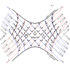
Figure 4: Causal diagram for the maximal analytical extension in the $E=1$ case. The two singularities and the two event horizons are shown together with lines of outgoing and ingoing null geodesics, drawn in red and blue, respectively, and with lines of constant ${\mathcal{t}}^{\prime}$ and $\tau^{\prime}$. The contravariant normals to the ${\mathcal{t}}^{\prime}={\rm constant}$ and $\tau^{\prime}={\rm constant}$ hypersurfaces, i.e., $n^{{\mathcal{t}^{\prime}}\hskip 0.1424pta}$ and $n^{\tau^{\prime}\hskip 0.1424pta}$, respectively, are also shown, with their timelike character clearly exhibited. See text for more details.

Figure 5: Causal diagram for the maximal analytical extension in the $E=1.1$ case. The two singularities and the two event horizons are shown together with lines of outgoing and ingoing null geodesics, drawn in red and blue, respectively, and with lines of constant ${\mathcal{t}}^{\prime}$ and $\tau^{\prime}$. The contravariant normals to the ${\mathcal{t}}^{\prime}={\rm constant}$ and $\tau^{\prime}={\rm constant}$ hypersurfaces, i.e., $n^{{\mathcal{t}^{\prime}}\hskip 0.1424pta}$ and $n^{\tau^{\prime}\hskip 0.1424pta}$, respectively, are also shown, with their timelike character clearly exhibited. See text for more details.

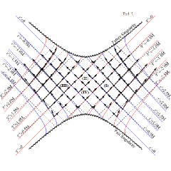
Figure 6: Causal diagram for the maximal analytical extension in the $E=1.5$ case. The two singularities and the two event horizons are shown together with lines of outgoing and ingoing null geodesics, drawn in red and blue, respectively, and with lines of constant ${\mathcal{t}}^{\prime}$ and $\tau^{\prime}$. The contravariant normals to the ${\mathcal{t}}^{\prime}={\rm constant}$ and $\tau^{\prime}={\rm constant}$ hypersurfaces, i.e., $n^{{\mathcal{t}^{\prime}}\hskip 0.1424pta}$ and $n^{\tau^{\prime}\hskip 0.1424pta}$, respectively, are also shown, with their timelike character clearly exhibited. See text for more details.

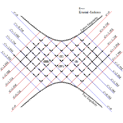
Figure 7: Causal diagram for the maximal analytical extension in the $E=\infty$ case, i.e., the Kruskal-Szekeres maximal extension. The two singularities and the two event horizons are shown together with lines of outgoing and ingoing null geodesics, drawn in red and blue, respectively, and with lines of constant $u^{\prime}\equiv\lim_{E\to\infty}{\mathcal{t}^{\prime}}$ and $v^{\prime}\equiv\lim_{E\to\infty}{\tau^{\prime}}$. In this $E=\infty$ case these two sets of lines coincide. The contravariant normals to the $u^{\prime}={\rm constant}$ and $v^{\prime}={\rm constant}$ hypersurfaces, i.e., $n^{u^{\prime}\hskip 0.1424pta}$ and $n^{v^{\prime}\hskip 0.1424pta}$, respectively, are also shown, with their null character clearly exhibited. See text for more details.

As it had to be, the lines of ${\mathcal{t}}^{\prime}={\rm constant}$ and $\tau^{\prime}={\rm constant}$ are tachyonic, i.e., spacelike hypersurfaces, a feature clearly seen by comparison of these lines with the ingoing and outgoing null geodesic lines, except for ${\mathcal{t}}^{\prime}=0$ and $\tau^{\prime}=0$ which are null lines representing the $r=2M$ event horizons of the solution that separate regions I, II, III, and IV. In the $E=\infty$ case, i.e., Kruskal-Szekeres, the spacelike lines turn into the null lines $u^{\prime}={\rm constant}$ and $v^{\prime}={\rm constant}$, with $u^{\prime}=0$ and $v^{\prime}=0$ being the event horizons separating regions I, II, III, and IV. One also sees that the contravariant normals $n^{{\mathcal{t}^{\prime}}\hskip 0.1424pta}$ and $n^{\tau^{\prime}\hskip 0.1424pta}$, are always inside the local light cone, and so the coordinates ${\mathcal{t}^{\prime}}$ and $\tau^{\prime}$ are timelike, except at the horizons where they are null. In the $E=\infty$ case, i.e., Kruskal-Szekeres, the contravariant normals $n^{u^{\prime}\hskip 0.1424pta}$ and $n^{v^{\prime}\hskip 0.1424pta}$ are null vectors always, and so the coordinates $u^{\prime}$ and $v^{\prime}$ are null, i.e., the ${\mathcal{t}^{\prime}}$ and $\tau^{\prime}$ timelike coordinates turned into the $u^{\prime}$ and $v^{\prime}$ null coordinates.

VII Conclusions

The scenario for maximally extend the Schwarzschild metric is now complete. Schwarzschild is the starting point. In the usual standard coordinates, also called Schwarzschild coordinates, its extension past the sphere $r=2M$ is cryptic, in any case is not maximal, and to exhibit it fully one needs two coordinate patches, altogether making it very difficult to obtain a complete interpretation. Departing from it, there is one branch alone, namely, the Painlevé-Gullstrand branch that works either with outgoing or with ingoing timelike congruences, or equivalently with outgoing or ingoing test particles placed over them, parameterized by their energy per unit mass $E$, and that in the $E\to\infty$ limit ends in the Eddington-Finkelstein retarded or advanced null coordinates, respectively. The Painlevé-Gullstrand branch, including its Eddington-Finkelstein $E=\infty$ endpoint, partially extends the Schwarzschild metric past $r=2M$, but it is not maximal, to have the full solution one needs two coordinate patches, which again inhibits the full interpretation of the solution. Then, from Painlevé-Gullstrand there are two bifucartion branches. One branch is the Novikov-Lemaître that uses the Painlevé-Gullstrand time coordinate and an appropriate radial comoving coordinate. This branch extends the Schwarzschild metric past $r=2M$, is maximal in the Novikov range $0<E<1$ and partial only in the Lemaître range $1\leq E<\infty$, ending, in the $E\to\infty$ limit, in Minkowski. The other branch is the one we found here, with the two analytically extended Painlevé-Gullstrand time coordinates, one related to outgoing, the other to ingoing timelike congruences. This branch extends the Schwarzschild metric past $r=2M$, is maximal and valid for $1\leq E<\infty$, and ends, for $E=\infty$, directly, or if wished, via the two analytically extended Eddington-Finkelstein retarded and advanced null coordinates, in the Kruskal-Szekeres maximal extension. The maximally extended solutions of the Schwarzschild metric allow for an easy and full interpretation of its complex spacetime structure.

Indeed, whereas the partial extensions of the Schwarzschild metric are of great interest to analyze gravitational collapse of matter and physical phenomena involving black holes where a future event horizon makes its appearance, and in certain instances to analyze time reversal white hole phenomena, the maximal extensions deliver the full solution, showing a model dynamic universe with two separate spacetime sheets, containing a past spacelike singularity, with a white hole region delimited by a past event horizon, that join at a dynamic nontraversable Einstein-Rosen bridge, or wormhole whose throat expands up to $r=2M$, to collapse into the inside of a future event horizon containing a black hole region with a future spacelike singularity separating again the two separate spacetime sheets of this model universe. Here, a family of maximal extensions of the Schwarzschild spacetime parameterized by the energy per unit mass $E$ of congruences of outgoing and ingoing timelike geodesics has been obtained. In this unified description, the Kruskal-Szekeres maximal extension of sixty years ago is seen here as the important, but now particular, instance of this $E$ family, namely, the one with $E=\infty$. This maximal description provides the link between Gullstrand-Painlevé and Kruskal-Szekeres.

Appendix: Details for the $E\to 1$ limit and the $E\to\infty$ Kruskal-Szekeres limit from the $E>1$ generic case

In order to see the continuity of the maximal extension parameterized by $E$, we take the generic $E>1$ case, and from it obtain directly the limit to the case $E=1$, and the limit to the case $E=\infty$, i.e., the Kruskal-Szekeres extension.

$E=1$ limit from $E>1$: Here we take the $E\to 1$ limit of Eqs. (13) and (14). We will do it term by term in each equation. For Eq. (13) we have: $\lim_{E\to 1}-4\left(\frac{2E^{2}-1+\frac{2M}{r}+2E\sqrt{E^{2}-1+\frac{2M}{r}}}{E^{2}-1+\frac{2M}{r}}\right)=-4\frac{(1+\sqrt{\frac{2M}{r}})^{2}}{\frac{2M}{r}}$; $\lim_{E\to 1}\exp{\left(-\frac{r}{2ME}\sqrt{E^{2}-1+\frac{2M}{r}}\right)}=\exp{\left(-\sqrt{\frac{r}{2M}}\right)}$; $\lim_{E\to 1}\left(\frac{\frac{M}{r}}{E^{2}-1+\frac{M}{r}+\sqrt{E^{2}-1}\sqrt{E^{2}-1+\frac{2M}{r}}}\right)^{\frac{2E^{2}-1}{2E\sqrt{E^{2}-1}}}=\left(1+2\sqrt{E^{2}-1}\sqrt{\frac{r}{2M}}\right)^{-\frac{1}{2\sqrt{E^{2}-1}}}=\exp\left[-\frac{1}{2\sqrt{E^{2}-1}}\ln\left(1+2\sqrt{E^{2}-1}\right.\right.\times\\ \left.\left.\times\sqrt{\frac{r}{2M}}\right)\right]=\exp{\left(-\sqrt{\frac{r}{2M}}\right)}$; $\lim_{E\to 1}-\frac{1}{M^{2}}\left(2E^{2}-1+\frac{2M}{r}+2E\sqrt{E^{2}-1+\frac{2M}{r}}\right)=-\frac{1}{M^{2}}\left(1+\sqrt{\frac{2M}{r}}\right)^{2}$;
$\lim_{E\to 1}\exp\left(-\frac{r}{2ME}\sqrt{E^{2}-1+\frac{2M}{r}}\right)=\exp{\left(-\sqrt{\frac{r}{2M}}\right)}$; $\lim_{E\to 1}\left(\frac{\frac{M}{r}}{E^{2}-1+\frac{M}{r}+\sqrt{E^{2}-1}\sqrt{E^{2}-1+\frac{2M}{r}}}\right)^{\frac{2E^{2}-1}{2E\sqrt{E^{2}-1}}}=\exp{\left(-\sqrt{\frac{r}{2M}}\right)}$; $\lim_{E\to 1}2\left(2E^{2}-1+\frac{2M}{r}\right)=2\left(1+\frac{2M}{r}\right)$. Thus, Eq. (13) is now $\mathrm{d}s^{2}=-4\frac{(1+\sqrt{\frac{2M}{r}})^{2}}{\frac{2M}{r}}\exp{\left(-2\sqrt{\frac{r}{2M}}\right)}\Big{[}-\frac{1}{M^{2}}\left(1+\sqrt{\frac{2M}{r}}\right)^{2}\times\\ \times\exp{\left(-2\sqrt{\frac{r}{2M}}\right)}(\tau^{\prime 2}\mathrm{d}{\mathcal{t}}^{\prime 2}+{\mathcal{t}}^{\prime 2}\mathrm{d}\tau^{\prime 2})+2\left(1+\frac{2M}{r}\right)\mathrm{d}{\mathcal{t}}^{\prime}\,\mathrm{d}\tau^{\prime 2}\Big{]}+r^{2}(\mathrm{d}\theta^{2}+\sin^{2}{\theta}\,\mathrm{d}\phi^{2})$. This is the line element found for the $E=1$ case, see Eq. (21). For Eq. (14) we have: $\lim_{E\to 1}\left(\frac{\frac{r}{2M}-1}{2E^{2}-1+\frac{2M}{r}+2E\sqrt{E^{2}-1+\frac{2M}{r}}}\right)\frac{2M}{r}=\frac{\sqrt{\frac{r}{2M}}-1}{\sqrt{\frac{r}{2M}}+1}$; $\lim_{E\to 1}\exp{\left(\frac{r}{2ME}\sqrt{E^{2}-1+\frac{2M}{r}}\right)}=\exp{\left(\sqrt{\frac{r}{2M}}\right)}$; $\lim_{E\to 1}\left[\frac{r}{M}\left(E^{2}-1+\frac{M}{r}+\sqrt{E^{2}-1}\sqrt{E^{2}-1+\frac{2M}{r}}\right)\right]^{\frac{2E^{2}-1}{2E\sqrt{E^{2}-1}}}=\allowbreak=\left(1+2\sqrt{E^{2}-1}\sqrt{\frac{r}{2M}}\right)^{\frac{1}{2\sqrt{E^{2}-1}}}=\exp\left[\frac{1}{2\sqrt{E^{2}-1}}\ln\left(1+2\sqrt{E^{2}-1}\sqrt{\frac{r}{2M}}\right)\right]=\exp{\left(\sqrt{\frac{r}{2M}}\right)}$. Thus, Eq (14) in the $E\to 1$ limit turns into $\frac{\sqrt{\frac{r}{2M}}-1}{\sqrt{\frac{r}{2M}}+1}\exp{\left(2\sqrt{\frac{r}{2M}}\right)}=-\frac{{\mathcal{t}}^{\prime}}{M}\frac{\tau^{\prime}}{M}$. This is indeed Eq. (22).

$E\to\infty$ limit from $E>1$, the Kruskal-Szekeres line element: Here we take the $E\to\infty$ limit of Eqs. (13) and (14). We will do it term by term in each equation. For Eq. (13) we have: $\lim_{E\to\infty}-4\left(\frac{2E^{2}-1+\frac{2M}{r}+2E\sqrt{E^{2}-1+\frac{2M}{r}}}{E^{2}-1+\frac{2M}{r}}\right)=-16$; $\lim_{E\to\infty}\exp{\left(-\frac{r}{2ME}\sqrt{E^{2}-1+\frac{2M}{r}}\right)}=\exp{\left(-\frac{r}{2M}\right)}$; $\lim_{E\to\infty}\left(\frac{M}{r}\,\frac{1}{E^{2}-1+\frac{M}{r}+\sqrt{E^{2}-1}\sqrt{E^{2}-1+\frac{2M}{r}}}\right)^{\frac{2E^{2}-1}{2E\sqrt{E^{2}-1}}}=\frac{M}{r}\frac{1}{2E^{2}}$; $\lim_{E\to\infty}-\frac{1}{M^{2}}\left(2E^{2}-1+\frac{2M}{r}+2E\sqrt{E^{2}-1+\frac{2M}{r}}\right)=\allowbreak=-\frac{4E^{2}}{M^{2}}$; $\lim_{E\to\infty}\exp{\left(-\frac{r}{2ME}\sqrt{E^{2}-1+\frac{2M}{r}}\right)}=\exp{\left(-\frac{r}{2M}\right)}$; $\lim_{E\to\infty}\left(\frac{\frac{M}{r}}{E^{2}-1+\frac{M}{r}+\sqrt{E^{2}-1}\sqrt{E^{2}-1+\frac{2M}{r}}}\right)^{\frac{2E^{2}-1}{2E\sqrt{E^{2}-1}}}=\allowbreak=\frac{M}{r}\frac{1}{2E^{2}}$; $\lim_{E\to\infty}2\left(2E^{2}-1+\frac{2M}{r}\right)=4E^{2}$. Thus, Eq (13) is now $\mathrm{d}s^{2}=-16\exp{\left(-\frac{r}{2M}\right)}\frac{M}{r}\frac{1}{2E^{2}}\Big{[}-\frac{4E^{2}}{M^{2}}\exp{\left(-\frac{r}{2M}\right)}\frac{M}{r}\times\\ \times\frac{1}{2E^{2}}(v^{\prime 2}\mathrm{d}u^{\prime 2}+u^{\prime 2}\mathrm{d}v^{\prime 2})+4E^{2}\mathrm{d}u^{\prime}\mathrm{d}v^{\prime}\,\Big{]}+r^{2}(\mathrm{d}\theta^{2}+\sin^{2}{\theta}\,\mathrm{d}\phi^{2})$, where for convenience of notation we have redefined the coordinates, $u^{\prime}\equiv{\mathcal{t}}^{\prime}$ and $v^{\prime}\equiv\tau^{\prime}$. Implementing definitely the $E\to\infty$ limit, the term in $(v^{\prime 2}\mathrm{d}u^{\prime 2}+u^{\prime 2}\mathrm{d}v^{\prime 2})$ vanishes and one gets, $\mathrm{d}s^{2}=-\frac{32M}{r}\exp{\left(-\frac{r}{2M}\right)}\mathrm{d}u^{\prime}\mathrm{d}v^{\prime}+r^{2}(\mathrm{d}\theta^{2}+\sin^{2}{\theta}\,\mathrm{d}\phi^{2})$. This is Eq.(29), i.e., the Kruskal-Szekeres line element. For Eq. (14) we have: $\lim_{E\to\infty}\left(\frac{\frac{r}{2M}-1}{2E^{2}-1+\frac{2M}{r}+2E\sqrt{E^{2}-1+\frac{2M}{r}}}\right)\frac{2M}{r}=\frac{\frac{r}{2M}-1}{4E^{2}}\frac{2M}{r}$; $\lim_{E\to\infty}\exp{\left(\frac{r}{2ME}\sqrt{E^{2}-1+\frac{2M}{r}}\right)}=\allowbreak=\exp{\left(\frac{r}{2M}\right)}$; $\lim_{E\to\infty}\left[\frac{r}{M}\left(E^{2}-1+\frac{M}{r}+\sqrt{E^{2}-1}\sqrt{E^{2}-1+\frac{2M}{r}}\right)\right]^{\frac{2E^{2}-1}{2E\sqrt{E^{2}-1}}}=\dfrac{r}{M}\,2E^{2}$. Thus, redefining for convenience of notation the coordinates ${\mathcal{t}}^{\prime}$ and $\tau^{\prime}$ as $u^{\prime}\equiv{\mathcal{t}}^{\prime}$ and $v^{\prime}\equiv\tau^{\prime}$, Eq (14) in the $E\to\infty$ limit turns into $\left(\frac{r}{2M}-1\right)\exp{\left(\frac{r}{2M}\right)}=-\frac{u^{\prime}}{M}\frac{v^{\prime}}{M}$. This is Eq. (30), i.e., the Kruskal-Szekeres implicit definition of $r$ in terms of $u^{\prime}$ and $v^{\prime}$. Seen through this direct limiting procedure, the Kruskal-Szekeres solution is indeed a particular case of the $E$ family of maximal extensions. In no place there was explicit need to resort to Eddington-Finkelstein null coordinates and their analytical extended versions.

References

(1)
K. Schwarzschild, “Über das Gravitationsfeld eines Massenpunktes nach der
Einsteinschen Theorie”, Sitzungsberichte der Königlich
Preussischen Akademie Wissenschaften 1916,
189 (1916).
(2)
J. Droste, “The field of a single centre in Einstein’s theory of
gravitation and the motion of a particle in that field”, Koninklijke
Nederlandsche Akademie van Wetenschappen Proceedings 19, 197
(1917).
(3)
D. Hilbert, “Die Grundlagen der Physik (Zweite Mitteilung)”,
Nachrichten von der Gesellschaft der Wissenschaften zu Göttingen,
Mathematisch-Physikalische Klasse 1917, 53 (1917).
(4)
G. D. Birkhoff,
Relativity and Modern Physics
(Harvard University Press, Cambridge Massachusetts 1923).
(5)
A. Einstein and N. Rosen, “The particle problem in the
general theory of relativity”, Phys. Rev. 48, 73
(1935).
(6)
C. W. Misner and J. A. Wheeler, “Classical physics as geometry:
Gravitation, electromagnetism, unquantized charge, and mass as
properties of curved empty space”, Annals of Physics 2,
525 (1957).
(7)
M. S. Morris and K. S. Thorne, “Wormholes in spacetime and their use
for interstellar travel: A tool for teaching general relativity”,
Am. J. Phys. 56, 395 (1988).
(8)
J. P. S. Lemos, F. S. N. Lobo, and S. Q. de Oliveira, “Morris-Thorne
wormholes with a cosmological constant”,
Phys. Rev. D 68, 064004 (2003); arXiv:gr-qc/0302049.
(9)
E. Guendelman, E. Nissimov, S. Pacheva, and M. Stoilov.
“Einstein-Rosen bridge revisited and lightlike thin-shell wormholes”,
Bulgarian Journal of Physics 44, 85 (2017);
arXiv:1611.04336 [gr-qc].
(10)
P. Painlevé, “La mécanique classique et la théorie de la
relativité”, Comptes Rendus de l’Académie des Sciences 173,
677 (1921).
(11)
A. Gullstrand, “Allgemeine Lösung des statischen Einkörperproblems
in der Einsteinschen Gravitationstheorie”,
Arkiv för Matematik, Astronomi och Fysik 16, 1 (1922).
(12)
R. Gautreau and B. Hoffmann,
“The Schwarzschild radial coordinate as a measure of proper distance”,
Phys. Rev. D 17, 2552 (1978).
(13)
M. K. Parikh and F. Wilczek,
“Hawking radiation as tunneling”,
Phys. Rev. Lett. 85 5042 (2000);
arXiv:hep-th/9907001.
(14)
K. Martel and E. Poisson,
“Regular coordinate systems for Schwarzschild and other spherical
spacetimes”,
Am. J. Phys. 69, 476 (2001); arXiv:gr-qc/0001069.
(15)
J. Natário,
“Painlevé-Gullstrand coordinates for the Kerr solution”,
Gen. Relativ. Gravit. 41, 2579 (2009);
arXiv:0805.0206 [gr-qc].
(16)
T. K. Finch,
“Coordinate families for the Schwarzschild geometry
based on radial timelike geodesics”,
Gen. Relativ. Gravit. 47, 56 (2015); arXiv:1211.4337 [gr-qc].
(17)
C. MacLaurin, “Schwarzschild spacetime under generalised
Gullstrand-Painlevé slicing”, in Einstein equations: Physical
and Mathematical Aspects of General Relativity, edited by
S. Cacciatori, B. Güneysu, and S. Pigola (Birkhäuser, Cham,
Switzerland 2019), p. 267; arXiv:1911.05988 [gr-qc].
(18)
G. Lemaître, “L’Univers en expansion”,
Annales de la Société Scientifique
de Bruxelles 53A, 51 (1933).
(19)
I. D. Novikov, Early Stages of the Evolution of the Universe
(Doctoral Dissertation, Sternberg
Astro-Astronomical Institute, Moscow 1963).
(20)
J. R. Oppenheimer and H. Snyder,
“On continued gravitational contraction”,
Phys. Rev. 56, 455 (1939).
(21)
Ya. B. Zel’dovich and I. D. Novikov,
Relativistic Astrophysics Volume 1:
Stars and Relativity
(University of Chicago Press, Chicago 1971).
(22)
R. Gautreau,
“On Kruskal-Novikov co-ordinate systems”,
Il Nuovo Cimento B 56, 49 (1980).
(23)
A. Krasiński, Inhomogeneous Cosmological Models
(Cambridge University Press, Cambridge 1997).
(24)
M. Blau,
Lecture Notes on General Relativity
(Author edition, Geneva 2014).
(25)
A. S. Eddington, “A comparison of Whitehead’s and Einstein’s
formula”, Nature 113, 192 (1924).
(26)
D. Finkelstein, “Past-future asymmetry of the gravitational field of
a point particle”, Phys. Rev. 110, 965 (1958).
(27)
R. Penrose, “Structure of space-time”, in Battelle Rencontres
1967, edited by C. M. DeWitt and J. A. Wheeler (Benjamin, New York
1968), p. 121.
(28)
M. Alcubierre and B. Brügmann, “Simple excision of a black hole in
3+1 numerical relativity”, Phys. Rev. D 63, 104006 (2001);
arXiv:gr-qc/0008067.
(29)
R. J. Adler, J. D. Bjorken, P. Chen, and J. S. Liu,
“Simple analytic models of gravitational collapse”,
Am. J. Phys. 73, 1148 (2005); arXiv:gr-qc/0502040.
(30)
E. Babichev, V. Dokuchaev, and Yu. Eroshenko,
“Backreaction of accreting matter onto a black hole
in the Eddington-Finkelstein coordinates”,
Class. Quantum Grav. 29, 115002 (2012);
arXiv:1202.2836 [gr-qc].
(31)
S. Abdolrahimi, D. N. Page, and C. Tzounis,
“Ingoing Eddington-Finkelstein metric of an evaporating black hole”,
Phys. Rev. D 100, 124038 (2019);
arXiv:1607.05280 [hep-th].
(32)
C. Gooding and W. G. Unruh, “Inflying perspectives of reduced phase
space”, Phys. Rev. D 100, 026010 (2019) arXiv:1902.04211
[gr-qc].
(33)
M. Kruskal, “Maximal extension of Schwarzschild metric”, Phys. Rev.
119, 1743 (1959).
(34)
G. Szekeres, “On the singularities of a Riemannian manifold”,
Publicationes Mathematicae Debrecen 7, 285 (1959).
(35)
R. W. Fuller and J. A. Wheeler,
“Causality and multiply connected space-time”,
Phys. Rev. 128, 919 (1962).
(36)
J. Synge, “The gravitational field of a particle”, Proceedings of
the Royal Irish Academy, Section A: Mathematical and Physical Sciences
53,
83 (1950).
(37)
C. Fronsdal,
“Completion and embedding of the Schwarzschild solution”,
Phys. Rev. 116, 778 (1959).
(38) S. W. Hawking and G. F. R. Ellis,
The Large Scale Structure
of Space-Time (Cambridge University Press, Cambridge
1973).
(39)
C. W. Misner, K. S. Thorne, and J. A. Wheeler,
Gravitation (W. H. Freeman, San Francisco 1973).
(40)
R. M. Wald,
General Relativity
(Chicago University Press, Chicago 1984).
(41)
R. D’Inverno,
Introducing Einstein’s Relativity
(Oxford University Press, Oxford 1992).
(42)
K. A. Bronnikov and S. G. Rubin,
Black Holes, Cosmology, and Extra Dimensions
(World Scientific, Singapore 2013).
(43)
P. T. Chruściel, Elements of General Relativity (Birkhäuser,
Cham, Switzerland 2020).
(44)
O. B. Zaslavskii,
“Acceleration of particles by acceleration horizons”,
Phys. Rev. D 88, 104016 (2013); arXiv:1301.2801 [gr-qc].
(45)
L. Hodgkinson, J. Louko, and A. C. Ottewill,
“Static detectors and circular-geodesic detectors
on the Schwarzschild black hole”,
Phys. Rev. D 89, 104002 (2014); arXiv:1401.2667 [gr-qc].
(46)
J. P. S. Lemos, “Naked singularities:
Gravitationally collapsing configurations of dust or radiation in
spherical symmetry - a unified treatment”, Phys. Rev. Lett.
68, 1447 (1992).