The ASAS-SN Catalog of Variable Stars VIII:
“Dipper” Stars in the Lupus Star-Forming Region

Abstract

Some young stellar objects such as T Tauri-like “dipper" stars vary due to transient partial occultation by circumstellar dust, and observations of this phenomenon inform us of conditions in the planet-forming zones close to these stars. Although many dipper stars have been identified with space missions such as Kepler/K2, ground-based telescopes offer longer term and multi-wavelength perspectives. We identified 11 dipper stars in the Lupus star forming region in data from the All-Sky Automated Survey for SuperNovae (ASAS-SN), and further characterized these using observations by the Las Cumbres Global Observatory Telescope (LCOGT) and the Transiting Exoplanet Survey Satellite (TESS), as well as archival data from other missions. Dipper stars were identified from a catalog of nearby young stars and selected based on the statistical significance, asymmetry, and quasi-periodicity or aperiodicity of variability in their ASAS-SN light curves. All 11 stars lie above or red-ward of the zero-age main sequence and have infrared excesses indicating the presence of full circumstellar disks. We obtain reddening-extinction relations for the variability of 7 stars using our combined ASAS-SN-TESS and LCOGT photometry. In all cases the slopes are below the ISM value, suggesting larger grains, and we find a tentative relation between the slope (grain size) and the $\text{K}_{\text{s}}-[22\>\mu\text{m}]$ infrared color regarded as a proxy for disk evolutionary state.

1 Introduction

Exoplanet science has seen much progress in recent years from both space- and ground-based observations alike (see the reviews by Petigura et al., 2013, Winn & Fabrycky, 2015, and Perryman, 2018). Discoveries by these surveys challenge us to reconcile the layout of the Solar System with what we observe in other planetary systems (e.g., Mordasini et al., 2015; Raymond et al., 2018). One of the biggest obstacles to progress is our limited knowledge of protoplanetary disk structure and the interactions between the disk and the central Young Stellar Object (YSO) (e.g., Morbidelli & Raymond, 2016). While Kepler found many planets within $\lesssim 1$ AU of stars, protoplanetary disks are generally not resolved at this scale by current telescopes, including the Atacama Large Millimeter Array ($\sim$5-10 au). Observations of YSO variability offer us a complementary view of phenomena around these stars at separations corresponding to the equivalent Keplerian orbital periods (Cody & Hillenbrand, 2018; Hedges et al., 2018; Ansdell et al., 2019).

YSO variability is divided into three classes (I–III; Herbst et al., 1994). Each class provides different insight into conditions on or around young stars: Type I, sinusoidal patterns are caused by the rotation of star spots; Type II, episodic “bursting" events are caused by increases in accretion onto the star; and Type III, dimming events are caused by occulting circumstellar matter. In this paper we focus on Type III variables. UX Orionis stars (UXORs), Herbig Ae/Be stars with occulting circumstellar dust, are a well-known example of this phenomenon (e.g., Co Ori, Davies et al., 2018). Lower mass ($M\lesssim 1$ M_⊙) T Tauri stars also exhibit dimming due to occulting dust. These were first found in ground-based observations, (e.g., AA Tau, Bouvier et al., 1999) but surveys by space telescopes such as Kepler/K2 have led to the discovery of many more such variables, which have become colloquially known as “dipper" stars (e.g., Cody & Hillenbrand, 2010; Morales-Calderón et al., 2011; Cody et al., 2014; Stauffer et al., 2015; Ansdell et al., 2016a, 2018a; Cody & Hillenbrand, 2018; Hedges et al., 2018). Unlike UXORs, dipper stars are T Tauri stars which exhibit dimming events ranging from quasi-periodic to completely episodic. The observable difference between UXORs and dippers are the dip timescale, occurrence, and depth, which for dippers are shorter, more frequent, and shallower, respectively, possibly because the inner edge of the dust disk is closer to lower-luminosity dippers (Kennedy et al., 2017). Dippers typically fade from tens of percent to multiple mag for about one day. Dipper variability is believed to be caused by transiting dust, probably associated with the inner regions of a nearly edge-on disk (Stauffer et al., 2015; Bodman et al., 2017). Alternative explanations such as exocomets (Boyajian et al., 2016) or dusty disk winds (Tambovtseva & Grinin, 2008; Bans & Königl, 2012) have also been proposed. Additional studies of dipper stars are needed to distinguish between the differing models.

While space telescopes such as Kepler provided high precision and cadence, their temporal baselines are limited to weeks (Spitzer and TESS) or months (K2), and survey only a small fraction of the sky at a time. CoRoT, Spitzer, and TESS conducted individual pointed observations, and the K2 mission was restricted to the ecliptic plane, and the Taurus and Upper Scorpius star-forming regions. Ground-based observatories such as the Kilodegree Extremely Little Telescope (KELT; Pepper et al., 2007) or the Palomar Transient Factory (PTF; Law et al., 2010) have been used to survey YSOs, e.g. Rodriguez et al. (2013); Rodriguez et al. (2016, 2017); Osborn et al. (2017); Ansdell et al. (2018a) and van Eyken et al. (2011); Findeisen et al. (2013), respectively. KELT had the advantage of all-sky coverage, but was limited to bright stars (8<V<12 mag). PTF had a deeper limiting magnitude ($\sim 20$ mag), but surveyed only the North American Nebula complex and the 25 Ori region. The successor to PTF, the Zwicky Transient Factory (Graham et al., 2019; Bellm et al., 2019), has expanded coverage to the entire night sky visible by Palomar.

Here we perform a search for variable YSOs in the Lupus region using the All-Sky Automated Survey for SuperNovae (ASAS-SN; Shappee et al., 2014; Kochanek et al., 2017) as part of a larger survey of transient objects. While ASAS-SN has discovered variable YSOs in the past (e.g., Holoien et al., 2014; Sicilia-Aguilar et al., 2017), the standard pipeline intentionally does not trigger on known objects or low amplitude variability. ASAS-SN offers photometric data of the entire sky from late 2012 to mid 2018 in the V band, and from late 2017 to present in the g band. The combination of a long baseline and all-sky coverage allows for large surveys of many different types of variability. While the ASAS-SN cadence is slower than K2 or KELT (typically once per day), ASAS-SN data provides a far wider sky coverage than K2, and has a deeper limiting magnitude than KELT. Additionally, ASAS-SN’s large longitude coverage allows for observations of the same source by multiple telescopes. As an example, ASAS-SN data has already been successfully used to identify variable stars (Jayasinghe et al., 2018, 2019d, 2019c; Pawlak et al., 2019; Jayasinghe et al., 2019e), derive period–luminosity relationships for $\delta$ Scuti stars (Jayasinghe et al., 2019a), identify M-dwarf flares (Rodríguez Martínez et al., 2019), study contact binaries (Jayasinghe et al., 2019b), and to examine the long-term variability of Boyajian’s Star (Simon et al., 2018) and compare it with the dipper phenomenon (Schmidt, 2019). Finally, ASAS-SN has recently identified a potential new “Boyajian’s Star" analog exhibiting rapid dimming events, nicknamed Zachy’s Star (Way et al., 2019).

The constellation Lupus comprises multiple $1$–$3$ Myr-old regions of low-mass star formation near the Scorpius Centaurus OB association (see the review by Comerón, 2008). At a distance of $189\pm 13$ pc, it is one of the closest star-forming regions (Zucker et al., 2019). The Lupus III cloud in particular is home to many well-studied T Tauri stars such as RU Lup and EX Lup. Lupus was not surveyed by K2, KELT, or PTF. While there have been several recent studies on disk structure (e.g., Ansdell et al., 2016b, 2018b) and accretion (e.g., Nisini et al., 2018) in Lupus YSOs, no dippers have been identified.

Here we use ASAS-SN observations to identify and classify Lupus variable stars in section 2. We discuss follow-up observations of dipper sources in section 3, and investigate their infrared excesses and dust properties using multi-band photometry in section 4.

2 Identifying Dipper Candidates

As the starting point of this investigation, we compiled a catalog of all known candidate members of young associations, open clusters and moving groups within 150 pc based on the member lists of Torres et al. (2008), Malo et al. (2013), Riedel et al. (2017), and Gagné et al. (2018a), complemented by Zuckerman (2019), Fürnkranz et al. (2019), Oh et al. (2017), Faherty et al. (2018), Meingast & Alves (2019), Tang et al. (2019), Gagné & Faherty (2018), and Gagné et al. (2018b). Of these sources, 307 are members of the Lupus Star-Forming Region.

2.1 ASAS-SN Observations

The ASAS-SN network consists of 20 telescopes mounted on 5 fully-robotic mounts located at the Haleakalā Observatory, the Cerro Tololo International Observatory, McDonald Observatory, and the South African Astrophysical Observatory. Observations span from late 2012 to mid-2018 in the V band, and from late 2017 in the g band, providing $\sim 800$ epochs per source on average. Each science image consists of three dithered 90 s exposures taken using 14-cm aperture Nikon telephoto lenses and thinned back-illuminated CCDs with $8.\!\!^{\prime\prime}0$ pixels.

Images from ASAS-SN are processed by the fully-automated ASAS-SN pipeline using the ISIS image subtraction package (Alard & Lupton, 1998; Alard, 2000). The IRAF apphot package is used with a 2-pixel ($\approx 16.\!\!^{\prime\prime}0$) aperture to perform aperture photometry on the subtracted images to generate a differential light curve. The same aperture is used to perform photometry in the reference images, and the resulting fluxes are added back to the differential light curve. The photometry is then calibrated using stars in the AAVSO Photometric All-Sky Survey (Henden et al., 2015). The greatest proper motion measured by Gaia for the Lupus YSOs is only $53.68\pm 0.05$ mas/yr, so there was no need to take the proper motions into account given our temporal baseline.

There are known systematic offsets between ASAS-SN telescopes (Jayasinghe et al., 2018). To combine data from different telescopes for a given filter, we use the SciPy interp1d package (Jones et al., 2001) to interpolate the most sampled curve. We then calculate the median difference between this interpolated light curve and the dataset with the highest number of contemporaneous points. We add this difference to the second dataset, combine the light curves, and repeat the process until the data from all telescopes are aligned. This results in each source having a g-band and V-band light curve.

To decrease the likelihood of false positives in our variability search, the light curve of each star is processed as follows. First, we remove data points corresponding to images where the FHWM of the point spread function is greater than the 90th percentile value of each telescope. Next, non-detections are omitted from statistical calculations. Lastly, we remove the top and bottom 1% of detections to clip potential outliers.

Stars brighter than $10.5$ mag in $V$ and $11$ mag in $g$ are at risk of saturation in ASAS-SN. Approximately 40% of the stars in our target list are saturated. We removed these brighter sources from our sample. Inconsistent reference fluxes between telescopes yield discrepant magnitude ranges during variable events. This most often took the form of one telescope reporting a large range of magnitudes while simultaneous observations from another appear to “flatline" by comparison. Any sources that noticeably demonstrated this pattern were omitted. Applying these cuts reduces our sample size from 307 to 177. The V-band curves of all remaining sources are processed and analyzed as outlined in section 2.2. Our selection process is summarized in Table 1.

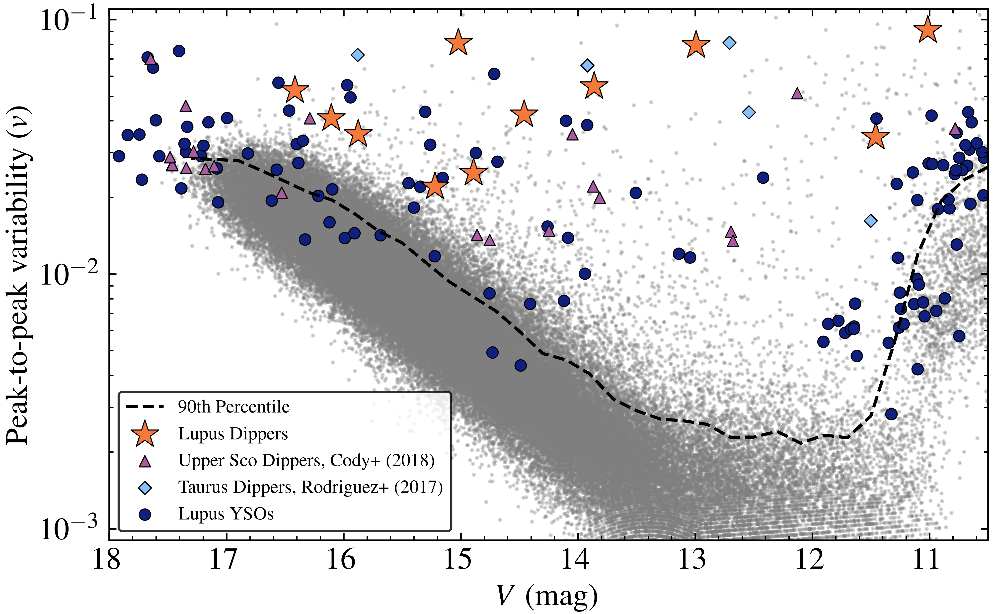
Figure 1: Peak-to-peak variability $v$ as a function of ASAS-SN V for our sample of YSOs. Stars flagged as dippers in Upper Scorpius (Table 2 of Cody & Hillenbrand, 2018) and Taurus (Table 3 of Rodriguez et al., 2017) that were present in our catalog are also shown. The dashed line corresponds to the 90th percentile of $v$ at a given magnitude based on the ASAS-SN V-band light curves of about 115,000 randomly selected field stars. Notice how saturation increases the average $v$ at magnitudes brighter than $\sim 11.5$. YSOs above the dashed line are considered variable. Out of the $177$ Lupus YSOs analyzed, $91$ pass this criterion for variability. The eleven Lupus dippers described in section 2.3 are marked by orange stars.

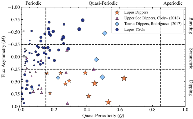
Figure 2: Flux Asymmetry vs Quasi-Periodicity for our sample of variable YSOs. The Flux Asymmetry $M$ is a measure of variability that is predominantly brightening ($M<0$), dimming ($M>0$), or symmetric ($M=0$). The Quasi-Periodicity $Q$ measures whether the variability is more periodic ($Q=0$) or stochastic ($Q>0$). The $Q-M$ space is divided into nine distinct regions to classify variability (Cody & Hillenbrand, 2018). Stars in Lupus that are in the Quasi-Periodic Dipper region are shown with orange stars. The area of each point is proportional to the peak-to-peak variability metric $v$. Stars flagged as dippers in Table 2 of Cody & Hillenbrand (2018) and Table 3 of Rodriguez et al. (2017) that were present in our sample are also shown.

2.2 Searching for Variability

In order to quantify variability, we use the peak-to-peak variability metric

$$v=\frac{(m_{i}-\sigma_{i})_{\text{max}}-(m_{i}+\sigma_{i})_{\text{min}}}{(m_{i}-\sigma_{i})_{\text{max}}+(m_{i}+\sigma_{i})_{\text{min}}},$$ (1)

from Sokolovsky et al. (2017), where $m_{i}$ is a measured magnitude and $\sigma_{i}$ is its associated uncertainty. For a comparison sample, we measured $v$ for the ASAS-SN V-band light curves of approximately $115,000$ randomly selected field stars. We calculate the 90th percentile of $v$ as a function of magnitude and selected the $91$ out of $177$ Lupus YSOs above this threshold as variable stars and retained them for further scrutiny. Figure 1 illustrates our selection of these sources based on $v$.

Table 1: Summary of cuts applied to Lupus YSO sample.

Criteria	Remaining Sample Size
Lupus members in YSO Catalog	307
Removal of Saturated Stars	177
$v>90$th Percentile	91
$Q>0.15$ and $M>0.25$	11

2.3 Classifications

Now that we have a selection of variable YSOs, we next classify their variability using the Quasi-Periodicity and Flux Asymmetry statistics defined in Cody et al. (2014). The Quasi-Periodicity

$$Q=\frac{(\sigma^{2}_{\text{resid}}-\sigma_{\text{phot}}^{2})}{(\sigma^{2}_{m}-\sigma_{\text{phot}}^{2})},$$ (2)

quantifies the degree to which variability is periodic or stochastic. Here $\sigma_{\text{phot}}$ is the estimated photometric uncertainty, $\sigma^{2}_{m}$ is the variance of the original light curve, and $\sigma^{2}_{\text{resid}}$ is the variance of the residual light curve after subtracting the dominant periodic signal. For a perfectly periodic signal, the variance of the residual is equivalent to photometric noise, yielding $Q\approx 0$.

To produce the residual curve, we create a window function (Dirac Comb) out of the original light curve, i.e. values of 1 when an observation takes place and values of 0 elsewhere. We utilize Astropy LombScargle (VanderPlas et al., 2012; VanderPlas & Ivezić, 2015) to find the periodograms of both the original curve and the Dirac Comb window function. We find all frequencies in the window function with a power greater than two standard deviations above the mean and ignore any peaks in the periodogram of the light curve within 0.03 Hz of the peaks in the window function. The curve is then phased using the remaining period with the highest power. We boxcar smooth this folded light curve with a window size of $25\%$ of the period and subtract the smoothed model from the folded curve. We define $\sigma_{\text{resid}}$ as the standard deviation of this residual curve.

The second metric to classify variability is Flux Asymmetry

$$M=\frac{\left<m_{10\%}\right>-m_{\text{med}}}{\sigma_{m}},$$ (3)

where $\left<m_{10\%}\right>$ is the mean of the top and bottom $10\%$ of magnitude measurements, $m_{\text{med}}$ is the median of all measurements, and $\sigma_{m}$ is the standard deviation of the light curve. $M$ determines whether the variability is predominantly brightening ($M$ < 0) or predominantly dimming ($M$ > 0).

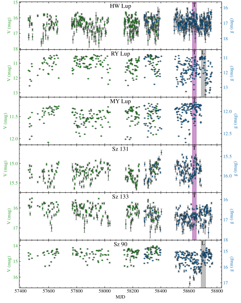
Figure 3: ASAS-SN light curves for the first six dippers in Lupus, in order of ascending RA. Measurements in the $V$-band are in green, while measurements in the $g$-band are in blue. The purple and gray shaded regions show the TESS (T) and LCOGT (L) observing periods, respectively, if applicable to the system. The vertical offset between the filters was found by interpolating the V-band data in the overlapping region. The correction is purely for presentation purposes.

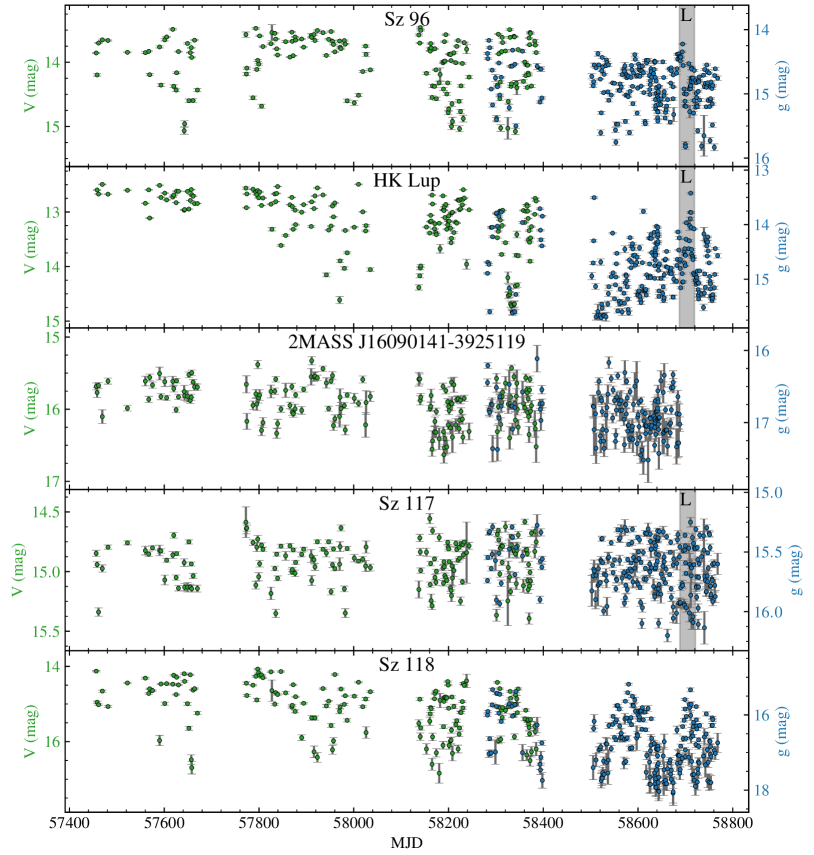
Figure 4: continued

ASAS-SN light curves for last five dippers in Lupus, in order of ascending RA. Style is the same as in Figure 3.

We calculate $Q$ and $M$ for the V-band data to separate the YSOs by variability type. The results are shown in Figure 2. The $Q-M$ space is divided into nine regions following Cody & Hillenbrand (2018). All eleven stars in the Quasi-periodic Dipping region ($0.15<Q<0.85$, $-0.25<M<0.25$) of Figure 2 were examined in detail, and their light curves are shown in Figure 3. The designations of all 91 variable Lupus YSOs are included in Table 2.

We also performed the same analysis for the ASAS-SN light curves of the dippers identified in Cody & Hillenbrand (2018) and Rodriguez et al. (2017) that were present in our catalog. These stars are also included in Figures 1, 2, and 8. The values of $Q$ and $M$ appear to be inconsistent between ASAS-SN and K2, in that there are Upper Scorpius stars identified in Cody & Hillenbrand (2018) as having dipper-like $Q$ and $M$ values based on K2 data that have non-dipper values based on ASAS-SN data. We suspect that the discrepant $Q$ and $M$ values are the result of differences in instrumental error and cadence. Ground telescopes such as ASAS-SN sample at timescales comparable to that of individual dipping episodes ($\sim$1 day), whereas K2 provides a much higher cadence (30 min) and greater precision. A more detailed comparison of $Q$ and $M$ in ASAS-SN as compared to K2 is left for future work. The ASAS-SN light curves of the flagged dippers (Figure 3) contain multiple episodic dimming events of up to 2-3 magnitudes, consistent with this variable type.

Table 2: Average ASAS-SN $V$ magnitudes, peak-to-peak variability, quasi-periodicity, flux asymmetry, and variability classification for all Lupus YSO members present in our catalog, as well as additional information for quasi-periodic dippers. Names of sources other than quasi-periodic dippers are given as ASAS-SN IDs, generated by their coordinates from the source catalogs (see section 2). The classifications are P, QP, and AP for periodic, quasi-periodic, and aperiodic respectively, and D, S, and B for dipper, symmetric, and burster, respectively. A complete list is available electronically.

Name	RA	Dec	SpT	V	$v$	Q	M	Designation	$A_{g}/A_{T}$	$A_{g}/A_{i}$
	deg	deg		mag
HW Lup	236.323	$-$34.308	M1${}^{\text{a}}$	16.416	0.053	0.390	0.321	QPD	$4.791\pm 0.018$	—
RY Lup	239.868	$-$40.364	G8${}^{\text{b}}$	11.015	0.091	0.448	0.536	QPD	$1.331\pm 0.001$	$1.405\pm 0.020$
MY Lup	240.186	$-$41.925	K0${}^{\text{c}}$	11.460	0.035	0.175	0.734	QPD	$1.840\pm 0.009$	—
Sz 131	240.206	$-$41.501	M2${}^{\text{a}}$	15.222	0.022	0.150	0.331	QPD	$2.998\pm 0.010$	—
Sz 133	240.873	$-$41.667	K2${}^{\text{a}}$	16.106	0.041	0.292	0.482	QPD	$1.784\pm 0.048$	—
Sz 90	241.792	$-$39.184	K7-M0${}^{\text{a}}$	14.460	0.042	0.269	0.542	QPD	—	$1.489\pm 0.054$
Sz 96	242.053	$-$39.143	—	13.863	0.055	0.411	0.792	QPD	—	$1.368\pm 0.063$
HK Lup	242.094	$-$39.079	M0.4${}^{\text{d}}$	12.993	0.079	0.531	0.914	QPD	—	$1.797\pm 0.051$
2MASS J1609	242.256	$-$39.420	M4${}^{\text{e}}$	15.877	0.035	0.240	0.326	QPD	—	—
Sz 117	242.435	$-$39.225	M2${}^{\text{a}}$	14.891	0.025	0.159	0.332	QPD	—	$1.084\pm 0.035$
Sz 118	242.453	$-$39.188	K6${}^{\text{a}}$	15.021	0.081	0.627	0.433	QPD	—	—
J140220.69$-$414451.1	210.586	$-$41.7475	—	10.679	0.027	$-$0.043	0.567	PD	—	—
J140600.39$-$411225.2	211.502	$-$41.207	—	11.452	0.041	0.120	$-$0.392	PB	—	—
J142048.90$-$474844.6	215.204	$-$47.8124	—	11.622	0.005	0.017	0.004	PS	—	—

${}^{\text{a}}$ Hughes et al. (1994);         ${}^{\text{b}}$ Gahm et al. (1989);         ${}^{\text{c}}$ Alcalá et al. (2017);         ${}^{\text{d}}$ Herczeg & Hillenbrand (2014);         ${}^{\text{e}}$ Romero et al. (2012)

3 Other Observations

Obscuration by dust produces reddening as well as extinction, and the relation between these depends on the grain size distribution and composition. Simultaneous multi-band observations of dipping events allow this to be investigated and compared between dipper stars and with the ISM. For example, monitoring in both Sloan $g$ and $i$ (or equivalently TESS $T$) bands allow the relation between the reddening $\Delta(g-i)$ with dimming $\Delta g$ to be measured, with

$$\frac{\Delta(g-i)}{\Delta g}=1-\frac{A_{i}}{A_{g}}$$ (4)

where $A_{g}$ and $A_{i}$ (or $A_{T}$) are the inferred extinction coefficients for the dust in the Sloan $g$ and $i$ (or TESS) bands (see section 4.3). To perform a higher-precision examination of individual dimming events and compare with contemporaneous ASAS-SN measurements, we utilize the observations made by TESS during Sector 12 and the Las Cumbres Observatory Global Telescope (LCOGT; Brown et al., 2013) 0.4 m telescopes in the $g$ and $i$ bands.

3.1 TESS

We extracted TESS light curves for five of the dipper candidates: HW Lup, RY Lup, MY Lup, Sz 131, and Sz 133. These observations were obtained during Sector 12, near the end of TESS’s initial survey of the Southern Hemisphere. The other dipper candidates were not observed by TESS.

We produce light curves from the TESS observations using an image subtraction pipeline optimized for use with the full-frame images (FFIs). This pipeline is very similar to that used to process ASAS-SN images and is also based on the ISIS package (Alard & Lupton, 1998; Alard, 2000). This method has become a standard technique for using TESS to study extragalactic transients like supernovae (Vallely et al., 2019; Fausnaugh et al., 2019) and the exceptional tidal disruption event ASASSN-19bt (Holoien et al., 2019). It has also been previously applied to the study of the EXor variable ESO-H$\alpha$ 99 by Hodapp et al. (2019).

For each source, we construct a reference image using 750-pixel-wide postage stamps cut from the first 100 Sector 12 FFIs of good quality. When building the reference images, we exclude FFIs with PSF widths or sky background levels above average for the sector as well as any FFIs associated with non-zero data quality flags. Using these reference images, we produce raw differential light curves for the five sources. However, Both TESS and ASAS-SN lightcurves these light curves only provide the change in flux relative to the value in the reference image. Equation 4 evaluated at two epochs $m$ and $n$ can be written as:

$$\frac{A_{T}}{A_{g}}=-\log_{10}\left(\frac{\Delta f_{T,m}+f_{T,0}}{\Delta f_{T,n}+f_{T,0}}\right)\left[\log_{10}\left(\frac{\Delta f_{g,m}+f_{g,0}}{\Delta f_{g,n}+f_{g,0}}\right)\right]^{-1}$$ (5)

This shows that the reddening-extinction slope depends not only on the TESS and ASAS-SN differential fluxes $df_{T,m}$ and $f_{g,m}$ but also on the corresponding reference fluxes $f_{T,0}$ and $f_{g,0}$. However, TESS’s PSF is about 16 times larger in area than ASAS-SN’s, so crowding affects TESS reference fluxes more often.

Crowding is not a problem for RY Lup and MY Lup, which are sufficiently bright ($T\sim 10$ mag) and well-isolated that we were able to obtain good measurements of the reference fluxes using aperture photometry. However, HW Lup, Sz 131, and Sz 133 are fainter and have nearby stars of comparable brightness. For these sources we estimated the reference flux using the ticgen software package (Jaffe & Barclay, 2017; Stassun et al., 2018). This method yields TESS magnitude estimates for HW Lup, Sz 131, and Sz 133 of 12.26, 11.56, and 13.86 mag, respectively. These magnitude estimates were converted into fluxes using a standard instrumental zero point of 20.44 electrons per second (Vanderspek et al., 2018). We then added flux to the raw differential light curves such that the median of the HW Lup, Sz 131, and Sz 133 observations matched this estimated reference value. This method has been used previously by Jayasinghe et al. (2019a) when studying $\delta$ Scuti stars with TESS. However, we caution that for non-periodic, inherently variable sources such as dippers, estimating the reference flux from ticgen should be made with higher-resolution contemporaneous observations with the TESS reference image. Because no such observations were made, the values of $1-A_{T}/A_{g}$ for HW Lup, Sz 131, and Sz 133 are influenced by the difference between the ticgen reported flux and the actual flux of the reference image. Future investigations can resolve this problem with a single epoch of higher resolution, multi-band, ground-based observations during a TESS campaign to calibrate the differential flux light curve.

The resultant TESS photometry is shown in Figure 5, along with the simultaneous ASAS-SN g-band observations. We note that the two short-duration features visible in the TESS light curve of HW Lup around MJD 58627 and MJD 58641 (marked with grey vertical bands) are almost certainly artifacts produced by scattered Earthshine. Excess background light due to scattered Earth and Moon light is a well-known nuisance characteristic of TESS observations, and the two spikes in the HW Lup light curve coincide with epochs of documented high background flux (see the Sector 12 TESS Data Release Notes for more details). Aside from these artifacts, the ASAS-SN and TESS data sets show generally excellent agreement.

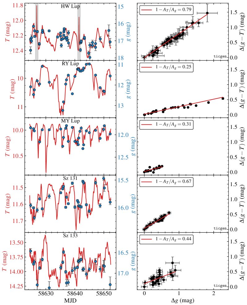
Figure 5: Left Panels: Simultaneous TESS (red) and ASAS-SN $g$ (blue) observations of five of the dipper candidates. The data from ASAS-SN has been vertically scaled to demonstrate the agreement with TESS on variability structure, with the right axis reporting the actual measured ASAS-SN magnitudes. The vertical gray regions indicate epochs when scattered Earthshine artifacts are dominant. TESS data from these epochs is excluded from the subsequent analysis. Right Panels: Reddening vs Dimming between ASAS-SN and TESS. The slope of the fitted line is equivalent to $1-A_{T}/A_{g}$. The value for interstellar dust is $1-A_{T}/A_{g}=0.38$. Sources marked with ticgen were located in crowded fields and could not have their reference flux measured directly. Consequently the slopes of these sources should be met with skepticism.

3.2 LCOGT

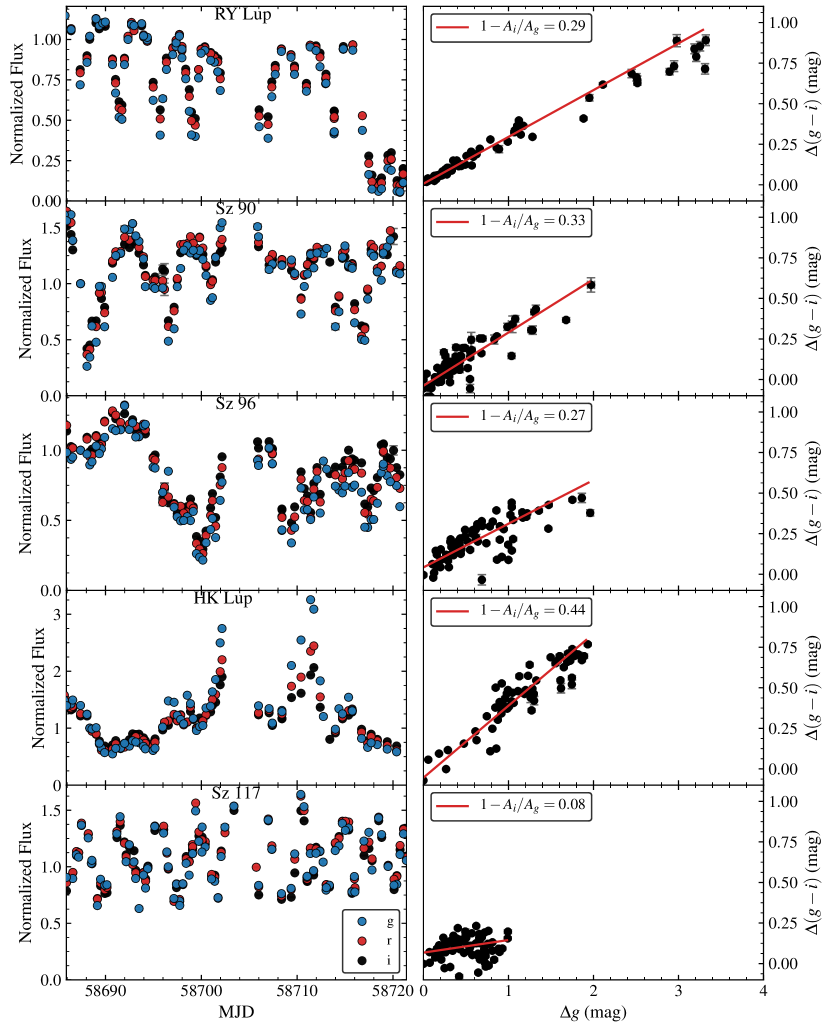
Figure 6: LCOGT SDSS $gri$ photometry of 5 of the dipper stars identified using ASAS-SN. Left Panels: Normalized light curves. Right Panels: Reddening vs. Dimming trends. Red lines are least-squares linear fits.

We also obtained $g$, $r$, and $i$ band observations of five Lupus dippers with the LCOGT 0.4-m telescope network, specifically the nodes at Suderland South Africa, CTIO, and Siding Spring, from 21 July, 2019 to 28 August, 2019. Images were acquired with the SBIG detector. Bias removal, image trimming, flat fielding, and photometry were performed with the BANZAI pipeline (McCully et al., 2018). Further analysis of the photometry was performed with custom differential scripts, choosing a set of reference stars with similar magnitudes in each case. RY Lup and Sz 117 were observed for 77 and 80 epochs, respectively, and Sz 90, Sz 96, and HK Lup were observed for 85 epochs (Figure 6).

4 ANALYSIS

4.1 Dippers in the Color-Magnitude Diagram

At the age of the Lupus molecular cloud, low-mass T Tauri stars such as these dippers have not reached the zero-age main sequence and should appear above the Zero-Age Main Sequence (ZAMS) in a color-magnitude diagram. We computed absolute magnitudes in the 2MASS $K_{s}$ band (Skrutskie et al., 2006) using parallaxes from Gaia DR2 (Gaia Collaboration et al., 2018) and show these with Gaia $B_{P}-R_{p}$ colors as orange stars in Figure 7. Note that Sz 133 lacks a DR2 parallax and does not appear. We compare these with predictions from Isochrones and Stellar Tracks (MIST; Dotter, 2016; Choi et al., 2016; Paxton et al., 2011; Paxton et al., 2013, 2015, 2018). Extinction by interstellar dust is comparatively low in the $K_{s}$ band relative to Gaia $B_{P}$ or $R_{p}$ and interstellar reddening will cause a star to move nearly horizontally to the right in this diagram, and so appear further above the ZAMS, giving the impression that they are both younger and less massive. Without spectroscopic follow-up, we cannot robustly estimate the $T_{\rm eff}$ and hence intrinsic $B_{p}-R_{p}$ color of these stars to reliably place them in this diagram to constrain their ages and masses. Moreover, the time-averaged visible-wavelength $B_{P}-R_{P}$ color reported by DR2 will be affected both by the mean level of circumstellar dust as well as spots on these young, active stars, which are not accounted for by the MIST models (Somers & Pinsonneault, 2015; Somers et al., 2020). However, we can obtain an approximate estimate of the stellar masses if we assume a minimum co-eval age. By adopting 2.2 Myr as the minimum co-eval age of the dipper stars, as well as a reddening relation for the ISM ($A_{\text{K}_{\text{s}}}=0.194\,\,\text{E}(B_{p}-R_{p})$; Yuan et al., 2013) we can project (dashed black lines and red dots in Figure 7) these stars onto the isochrone (dashed blue line) and estimate the minimum reddening and minimum masses of the stars. Most of the dippers have $M\lesssim 1\,\text{M}_{\odot}$ with the notable exception of RY Lup, where we obtain $M\sim 2.3\,\text{M}_{\odot}$ using this method. This is consistent with the picture of dipper stars as low mass T Tauri stars, to be distinguished from their higher mass UXOR Ae/Be-type cousins.

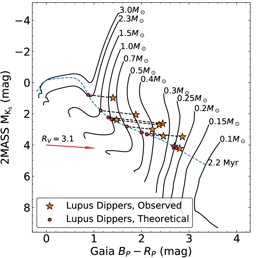
Figure 7: Gaia $B_{P}-R_{P}$ color vs. absolute $\text{M}_{\text{K}_{\text{s}}}$ color-mag diagram for ten of the dippers. Absolute magnitudes are obtained using distances from Bailer-Jones et al. (2018). The isochrone models are from MIST. By assuming an age of 2.2 Myr for the dippers and iteratively applying a reddening correction, we obtain rough estimates for stellar masses.

4.2 Infrared Excess and Disks

For young stars, excess emission in the infrared is indicative of the presence of a disk. By comparing a star’s absolute flux in the 2MASS $\text{K}_{\text{s}}$ band, which will be dominated by the photosphere, with their 12 ($W3$) and 22 ($W4$) $\mu$m fluxes from the Wide-field Infrared Survey Explorer (WISE; Wright et al., 2010; Mainzer et al., 2011), we can ascertain the presence of a disk and investigate its evolutionary state (Luhman & Mamajek, 2012). Figure 8 shows the $\text{K}_{\text{s}}-[12\>\mu\text{m}]$ vs. $\text{K}_{\text{s}}-[22\>\mu\text{m}]$ colors of the Lupus YSOs along with other reported dippers in Upper Scorpius and Taurus. The boundaries for disk types defined by Luhman & Mamajek (2012) are included. Young stars with “full" or classical T Tauri disks occupy the upper right hand portion of the figure. As the disk evolves, the star will lose its infrared excess. The relative rates at which $\text{K}_{\text{s}}-[22\>\mu\text{m}]$ and $\text{K}_{\text{s}}-[12\>\mu\text{m}]$ decrease are indicative of how and where the disk is evolving. All eleven dipper candidates show infrared excesses consistent with that of full disk-bearing YSOs, along with all but one of the previously reported dippers in our sample. This further supports a connection between the presence of a disk and the dipper phenomenon.

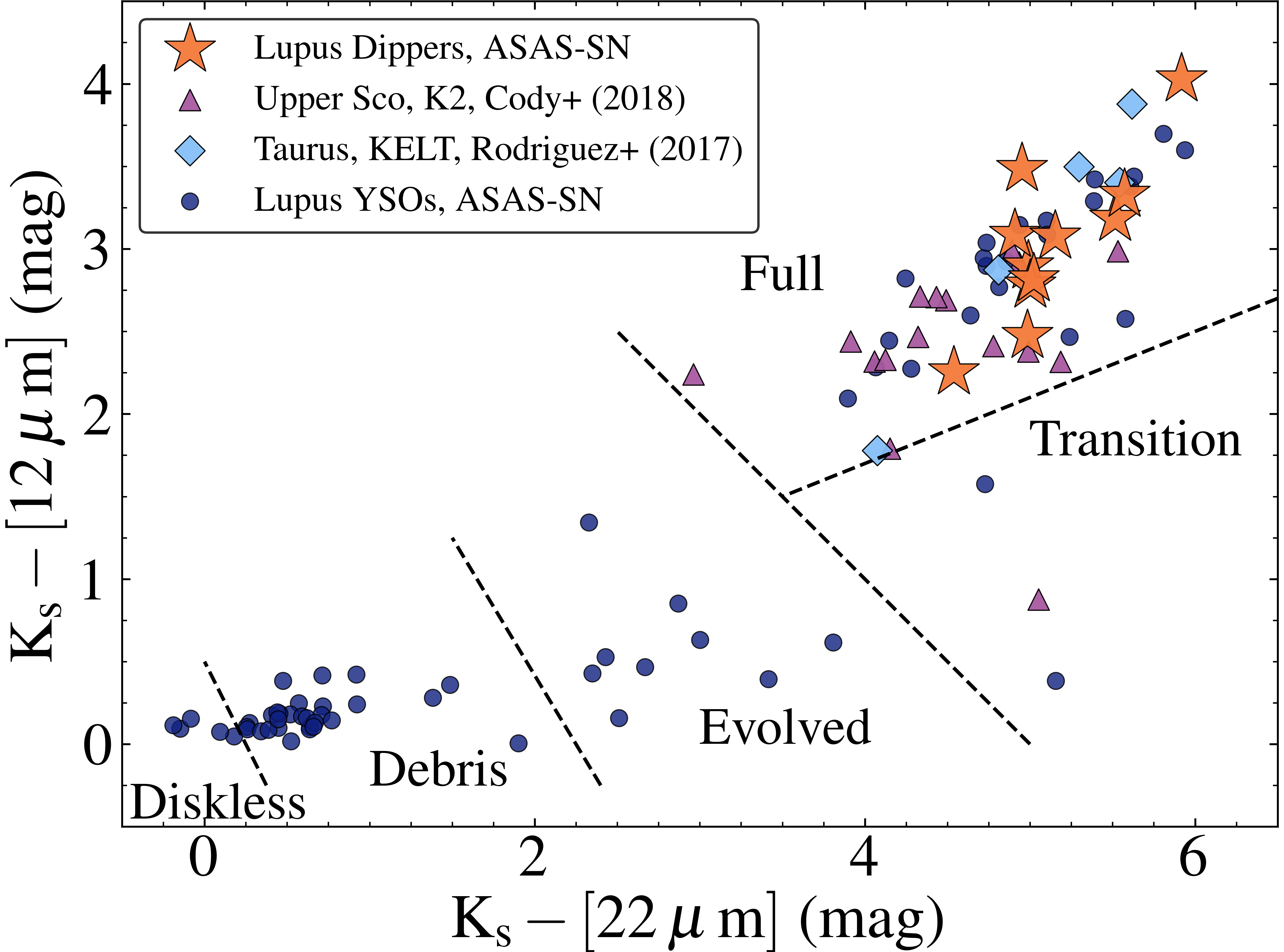
Figure 8: 2MASS–WISE color–color diagram. Zones characteristic of the different evolutionary stages of disks as defined by Luhman & Mamajek (2012) are demarcated by the dashed lines. The Lupus dippers are labelled alongside other known dippers. Other Lupus stars in our YSO catalog are shown in blue. The infrared excess of the dippers is consistent with dipping being related to the presence of a disk.

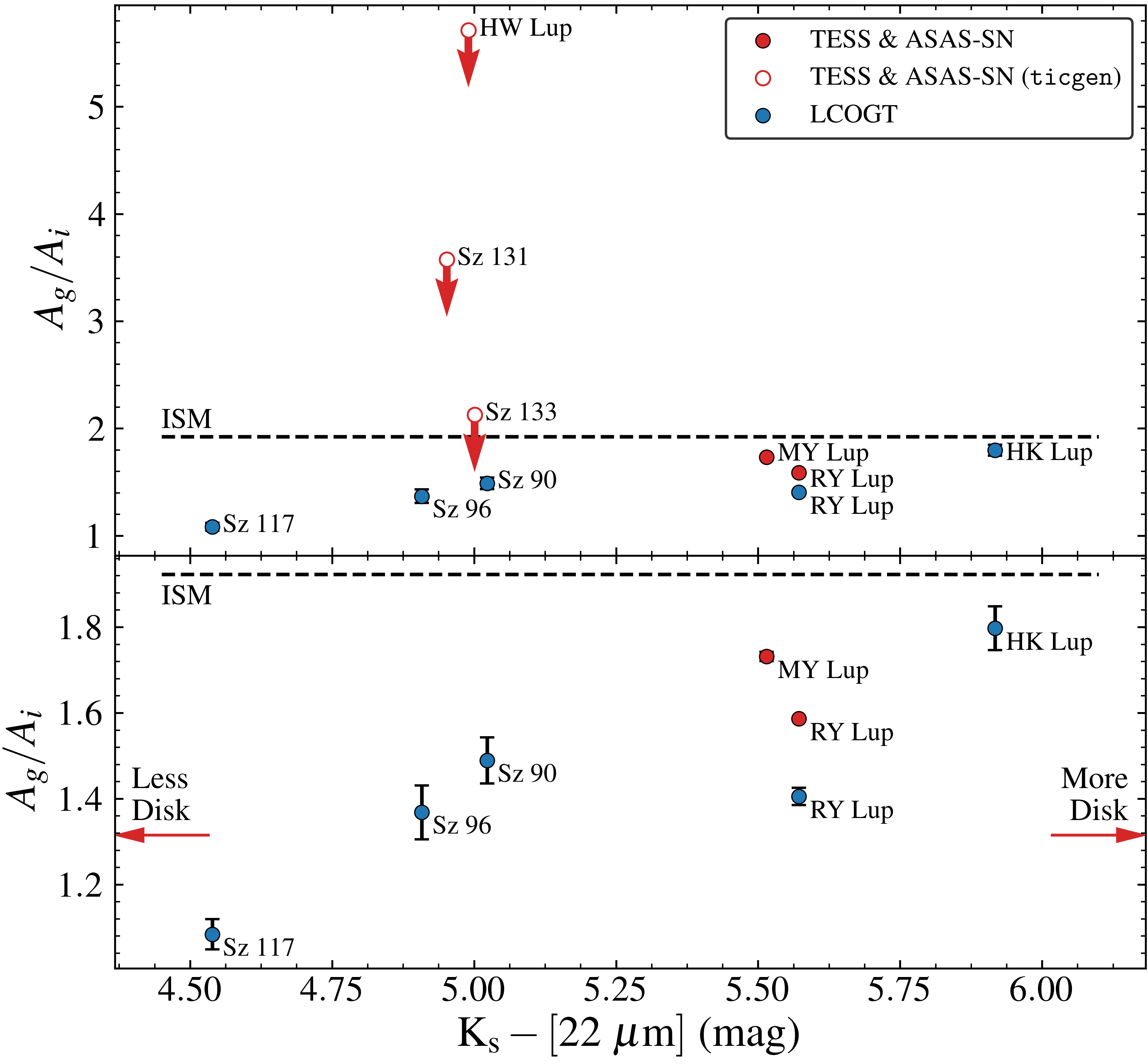
Figure 9: Top Panel: The dependence of the $A_{g}/A_{i}$ extinction ratio on the source’s IR excess. IR Excess is an indicator of excess emission due to a hot inner disk. We see a potential relation between the two, though additional data is needed. Slopes for HW Lup, Sz 131, and Sz 133 are shown as open points to reflect the possible unreliability of the values (see text). Bottom Panel: A zoomed view of the dippers with directly measured references fluxes.

4.3 Multi-Band Variability and Dust Properties

Simultaneous observations of young stellar variability in two or more band-passes provides a means of differentiating between different phenomena (e.g., flares, accretion, circumstellar dust). In the case of obscuration and reddening by circumstellar dust, it serves as an indicator of the grain size distribution (e.g., Herbst et al., 1994; Bouvier et al., 1999; Huang et al., 2019). The relative change (slope) in color (reddening) and magnitude (dimming) (Equation 4) depends on the characteristic grain size $d$ and composition. Dust dominated by small grains will produce steeper slopes (more reddening for a given amount of dimming) compared to dust dominated by larger grains, which in the limit of $d\gg\lambda$ will produce no reddening at all. The grain size distribution is affected by grain growth in the disks, and the slope of the trend in a color–magnitude plot is indicative of that history (e.g., Guo et al., 2018). UX Orionis stars exhibit reddening up to a point where the direct line of sight to the star is almost entirely obscured, causing scattered light that is comparatively blue to dominate, switching the sign of the slope (Bibo & The, 1990; Grinin et al., 1994). In contrast, the lack of reddening (and in fact slight bluing) by the repetitive dipper AA Tau has been explained by grains $>1\mu$m (Bouvier et al., 1999). Note that these plots are insensitive to zero-point offsets in magnitudes, since all values are differential.

Five Lupus dippers (HW Lup, RY Lup, MY Lup, Sz 131, Sz 133) were monitored simultaneously by the TESS mission and ASAS-SN. The TESS band-pass $T$ spans 600–1000 nm and is centered on the Cousins $I$-band (Ricker et al., 2014). Figure 5 shows the $g$-band ASAS-SN and TESS data, and the change in the $g-T$ color with $g$. Linear least-$\chi^{2}$ fits are shown as red lines. Based on the reddening $R$ values in Yuan et al. (2013) and Stassun et al. (2019), the expected slope of reddening due to interstellar dust is 0.38.

Light curves and $g-i$ versus $i$ reddening diagrams for the five stars (RY Lup, Sz 90, Sz 96, HK Lup, and Sz 117) observed with LCOGT are shown in Figure 6. In this case, the expected slope from interstellar dust is 0.48. In all cases the slope is less than, and sometimes significantly less than, the expected interstellar dust value. Only one star, RY Lup, was observed by all three telescope networks, but not all simultaneously. The TESS and LCOGT observations are not contemporaneous, with the former ending about 33 days before the beginning of the latter. The LCOGT slope (0.29) and TESS–ASAS-SN slope (0.25) are roughy consistent, with the smaller TESS–ASAS-SN slope (larger $A_{T}$ compared to $A_{i}$) consistent with the extension of the TESS bandpass to shorter wavelengths than the SDSS $i$ band filter. Values of $A_{g}/A_{i}$ and $A_{g}/A_{T}$, derived from these slops, are included in Table 2.

We can find no obvious correlation between the slope of the color–magnitude variation from our TESS–ASAS-SN or LCOGT observations and other properties of our disks such as the relative luminosity, the minimum wavelength of the infrared excess (Merín et al., 2008), the disk inclination or physical extent of dust and gas (if resolved) or the estimated dust/gas masses (Ansdell et al., 2016b, 2018b). However, we do see a possible correlation between the reddening slope and the infrared excess of the disk (WISE $22$ $\mu$m emission) relative to the photosphere (2MASS $\text{K}_{\text{s}}$ emission). HK Lup, MY Lup, and RY Lup have highest values of $A_{g}/A_{i}$ and ostensibly the smallest grains and also the largest infrared excess (Figure 9). The system with the lowest $22$ $\mu$m excess, Sz 117, also has little or no reddening, with $A_{i}/A_{g}$ near unity. We have included our TESS measurements of $A_{g}/A_{i}$ for HW Lup, Sz 131, and Sz 133, but we use open symbols and arrows for them in Figure 9 since the reference flux estimated using ticgen may not be reliable. Excluding these objects, the Spearman correlation coefficient of the data indicates a 97% probability that the two parameters, $A_{g}/A_{i}$ and $\text{K}_{\text{s}}-[22\>\mu\text{m}]$, are correlated.

A correlation between extinction coefficients and infrared excess could be explained if either (a) coalescence of a fixed mass of dust into larger grains produced both a flatter slope and less emitting area (and hence less emission), or (b) the growth of grains also proceeded contemporaneously with clearing of the disk. The two scenarios are mutually exclusive. With our small sample size (11 systems) and limited spectrophotometric data set we are unable to choose between these two possible explanations; more observations of a larger sample are clearly needed.

5 Summary

We have identified 11 dipper stars in the Lupus molecular cloud using ASAS-SN observations and a series of quantitative selection criteria that identified YSO members of Lupus, variable Lupus YSOs, and Lupus YSOs that varied in a manner consistent with dippers identified in other star-forming regions (Cody et al., 2014). All eleven stars are pre-main sequence, lying above the theoretical zero-age main sequence in a color-magnitude diagram. Their positions in the diagram are consistent with expectations for Lupus-age ($\sim$2 Myr) low-mass ($\lesssim$1 $M_{\odot}$) stars, but we are unable to estimate individual ages or masses due both to the lack of spectra and uncertainties in the effect of spots on theoretical models. All 11 dippers have infrared excesses consistent with a “full" T Tauri disk, as has been observed for other dipper stars (e.g., Ansdell et al., 2016a). Our findings expand the scope of the dipping phenomenon to yet another star-forming environment and epoch.

We used multi-wavelength time-series photometry of these dipper stars, combining ASAS-SN, TESS, and LCOGT observations, to measure the reddening by the occulting dust and thus infer something about the grain size. In all cases the amount of reddening was less, and thus the grain sizes larger, than that expected from ISM-like dust. Moreover, we find a tentative trend of decreasing reddening, and hence increasing grain size, with decreasing infrared excess, or equivalently more advanced evolutionary stages of the disk. This is consistent with a picture of grain growth with time in protoplanetary disks (Testi et al., 2014). These results need to be confirmed with larger and more in-depth studies, but highlight the synergy of ground- and space-based observations in the effort to better understand the structure and evolution of circumstellar disks and the planetary systems they spawn.

References

- Alard (2000) Alard C., 2000, A&AS, 144, 363
- Alard & Lupton (1998) Alard C., Lupton R. H., 1998, ApJ, 503, 325
- Alcalá et al. (2017) Alcalá J. M., et al., 2017, A&A, 600, A20
- Ansdell et al. (2016a) Ansdell M., et al., 2016a, ApJ, 816, 69
- Ansdell et al. (2016b) Ansdell M., et al., 2016b, ApJ, 828, 46
- Ansdell et al. (2018a) Ansdell M., et al., 2018a, MNRAS, 473, 1231
- Ansdell et al. (2018b) Ansdell M., et al., 2018b, ApJ, 859, 21
- Ansdell et al. (2019) Ansdell M., et al., 2019, Monthly Notices of the Royal Astronomical Society, 492, 572
- Bailer-Jones et al. (2018) Bailer-Jones C. A. L., Rybizki J., Fouesneau M., Mantelet G., Andrae R., 2018, AJ, 156, 58
- Bans & Königl (2012) Bans A., Königl A., 2012, ApJ, 758, 100
- Bellm et al. (2019) Bellm E. C., et al., 2019, PASP, 131, 018002
- Bibo & The (1990) Bibo E. A., The P. S., 1990, A&A, 236, 155
- Bodman et al. (2017) Bodman E. H. L., et al., 2017, MNRAS, 470, 202
- Bouvier et al. (1999) Bouvier J., et al., 1999, A&A, 349, 619
- Boyajian et al. (2016) Boyajian T. S., et al., 2016, MNRAS, 457, 3988
- Brown et al. (2013) Brown T. M., et al., 2013, PASP, 125, 1031
- Choi et al. (2016) Choi J., Dotter A., Conroy C., Cantiello M., Paxton B., Johnson B. D., 2016, ApJ, 823, 102
- Cody & Hillenbrand (2010) Cody A. M., Hillenbrand L. A., 2010, ApJS, 191, 389
- Cody & Hillenbrand (2018) Cody A. M., Hillenbrand L. A., 2018, AJ, 156, 71
- Cody et al. (2014) Cody A. M., et al., 2014, AJ, 147, 82
- Comerón (2008) Comerón F., 2008, in Reipurth B., ed., , Vol. 5, Handbook of Star Forming Regions, Volume II: The Southern Sky. Astronomical Society of the Pacific, Chapt. The Lupus Clouds, pp 295–350
- Davies et al. (2018) Davies C. L., Kreplin A., Kluska J., Hone E., Kraus S., 2018, MNRAS, 474, 5406
- Dotter (2016) Dotter A., 2016, ApJS, 222, 8
- Faherty et al. (2018) Faherty J. K., Bochanski J. J., Gagné J., Nelson O., Coker K., Smithka I., Desir D., Vasquez C., 2018, ApJ, 863, 91
- Fausnaugh et al. (2019) Fausnaugh M. M., et al., 2019, arXiv e-prints, p. arXiv:1904.02171
- Findeisen et al. (2013) Findeisen K., Hillenbrand L., Ofek E., Levitan D., Sesar B., Laher R., Surace J., 2013, ApJ, 768, 93
- Fürnkranz et al. (2019) Fürnkranz V., Meingast S., Alves J., 2019, A&A, 624, L11
- Gagné & Faherty (2018) Gagné J., Faherty J. K., 2018, ApJ, 862, 138
- Gagné et al. (2018a) Gagné J., et al., 2018a, ApJ, 856, 23
- Gagné et al. (2018b) Gagné J., Faherty J. K., Mamajek E. E., 2018b, ApJ, 865, 136
- Gahm et al. (1989) Gahm G. F., Fischerstrom C., Liseau R., Lindroos K. P., 1989, A&A, 211, 115
- Gaia Collaboration et al. (2018) Gaia Collaboration et al., 2018, A&A, 616, A1
- Graham et al. (2019) Graham M. J., et al., 2019, PASP, 131, 078001
- Grinin et al. (1994) Grinin V. P., The P. S., de Winter D., Giampapa M., Rostopchina A. N., Tambovtseva L. V., van den Ancker M. E., 1994, A&A, 292, 165
- Guo et al. (2018) Guo Z., et al., 2018, ApJ, 852, 56
- Hedges et al. (2018) Hedges C., Hodgkin S., Kennedy G., 2018, MNRAS, 476, 2968
- Henden et al. (2015) Henden A. A., Levine S., Terrell D., Welch D. L., 2015, in American Astronomical Society Meeting Abstracts #225. p. 33616
- Herbst et al. (1994) Herbst W., Herbst D. K., Grossman E. J., Weinstein D., 1994, AJ, 108, 1906
- Herczeg & Hillenbrand (2014) Herczeg G. J., Hillenbrand L. A., 2014, ApJ, 786, 97
- Hodapp et al. (2019) Hodapp K. W., et al., 2019, AJ, 158, 241
- Holoien et al. (2014) Holoien T. W.-S., et al., 2014, ApJ, 785, L35
- Holoien et al. (2019) Holoien T. W. S., et al., 2019, ApJ, 883, 111
- Huang et al. (2019) Huang P. C., et al., 2019, ApJ, 871, 183
- Hughes et al. (1994) Hughes J., Hartigan P., Krautter J., Kelemen J., 1994, AJ, 108, 1071
- Jaffe & Barclay (2017) Jaffe T. J., Barclay T., 2017, ticgen: A tool for calculating a TESS magnitude, and an expected noise level for stars to be observed by TESS., doi:10.5281/zenodo.888217, https://doi.org/10.5281/zenodo.888217
- Jayasinghe et al. (2018) Jayasinghe T., et al., 2018, MNRAS, 477, 3145
- Jayasinghe et al. (2019a) Jayasinghe T., et al., 2019a, arXiv e-prints, p. arXiv:1910.14187
- Jayasinghe et al. (2019b) Jayasinghe T., et al., 2019b, arXiv e-prints, p. arXiv:1911.09685
- Jayasinghe et al. (2019c) Jayasinghe T., et al., 2019c, MNRAS, 485, 961
- Jayasinghe et al. (2019d) Jayasinghe T., et al., 2019d, MNRAS, 486, 1907
- Jayasinghe et al. (2019e) Jayasinghe T., et al., 2019e, Monthly Notices of the Royal Astronomical Society, 491, 13
- Jones et al. (2001) Jones E., Oliphant T., Peterson P., et al., 2001, SciPy: Open source scientific tools for Python, http://www.scipy.org/
- Kennedy et al. (2017) Kennedy G. M., Kenworthy M. A., Pepper J., Rodriguez J. E., Siverd R. J., Stassun K. G., Wyatt M. C., 2017, Royal Society Open Science, 4, 160652
- Kochanek et al. (2017) Kochanek C. S., et al., 2017, PASP, 129, 104502
- Law et al. (2010) Law N. M., et al., 2010, in McLean I. S., Ramsay S. K., Takami H., eds, foo Vol. 7735, Ground-based and Airborne Instrumentation for Astronomy III. SPIE, pp 1411–1418, doi:10.1117/12.857400, https://doi.org/10.1117/12.857400
- Luhman & Mamajek (2012) Luhman K. L., Mamajek E. E., 2012, ApJ, 758, 31
- Mainzer et al. (2011) Mainzer A., et al., 2011, ApJ, 731, 53
- Malo et al. (2013) Malo L., Doyon R., Lafrenière D., Artigau É., Gagné J., Baron F., Riedel A., 2013, ApJ, 762, 88
- McCully et al. (2018) McCully C., et al., 2018, LCOGT/banzai: Initial Release, doi:10.5281/zenodo.1257560
- Meingast & Alves (2019) Meingast S., Alves J., 2019, A&A, 621, L3
- Merín et al. (2008) Merín B., et al., 2008, ApJS, 177, 551
- Morales-Calderón et al. (2011) Morales-Calderón M., et al., 2011, The Astrophysical Journal, 733, 50
- Morbidelli & Raymond (2016) Morbidelli A., Raymond S. N., 2016, Journal of Geophysical Research (Planets), 121, 1962
- Mordasini et al. (2015) Mordasini C., Mollière P., Dittkrist K. M., Jin S., Alibert Y., 2015, International Journal of Astrobiology, 14, 201
- Nisini et al. (2018) Nisini B., Antoniucci S., Alcalá J. M., Giannini T., Manara C. F., Natta A., Fedele D., Biazzo K., 2018, A&A, 609, A87
- Oh et al. (2017) Oh S., Price-Whelan A. M., Hogg D. W., Morton T. D., Spergel D. N., 2017, AJ, 153, 257
- Osborn et al. (2017) Osborn H. P., et al., 2017, MNRAS, 471, 740
- Pawlak et al. (2019) Pawlak M., et al., 2019, MNRAS, 487, 5932
- Paxton et al. (2011) Paxton B., Bildsten L., Dotter A., Herwig F., Lesaffre P., Timmes F., 2011, ApJS, 192, 3
- Paxton et al. (2013) Paxton B., et al., 2013, ApJS, 208, 4
- Paxton et al. (2015) Paxton B., et al., 2015, ApJS, 220, 15
- Paxton et al. (2018) Paxton B., et al., 2018, ApJS, 234, 34
- Pepper et al. (2007) Pepper J., et al., 2007, PASP, 119, 923
- Perryman (2018) Perryman M., 2018, The Exoplanet Handbook, 2 edn. Cambridge University Press
- Petigura et al. (2013) Petigura E. A., Howard A. W., Marcy G. W., 2013, Proceedings of the National Academy of Science, 110, 19273
- Raymond et al. (2018) Raymond S. N., Izidoro A., Morbidelli A., 2018, arXiv e-prints, p. arXiv:1812.01033
- Ricker et al. (2014) Ricker G. R., et al., 2014, Journal of Astronomical Telescopes, Instruments, and Systems, 1, 1
- Riedel et al. (2017) Riedel A. R., Blunt S. C., Lambrides E. L., Rice E. L., Cruz K. L., Faherty J. K., 2017, AJ, 153, 95
- Rodríguez Martínez et al. (2019) Rodríguez Martínez R., Lopez L. A., Shappee B. J., Schmidt S. J., Jayasinghe T., Kochanek C. S., Auchettl K., Holoien T. W. S., 2019, arXiv e-prints, p. arXiv:1912.05549
- Rodriguez et al. (2013) Rodriguez J. E., Pepper J., Stassun K. G., Siverd R. J., Cargile P., Beatty T. G., Gaudi B. S., 2013, AJ, 146, 112
- Rodriguez et al. (2016) Rodriguez J. E., et al., 2016, ApJ, 831, 74
- Rodriguez et al. (2017) Rodriguez J. E., et al., 2017, ApJ, 848, 97
- Romero et al. (2012) Romero G. A., Schreiber M. R., Cieza L. A., Rebassa-Mansergas A., Merín B., Smith Castelli A. V., Allen L. E., Morrell N., 2012, ApJ, 749, 79
- Schmidt (2019) Schmidt E. G., 2019, ApJ, 880, L7
- Shappee et al. (2014) Shappee B. J., et al., 2014, ApJ, 788, 48
- Sicilia-Aguilar et al. (2017) Sicilia-Aguilar A., et al., 2017, A&A, 607, A127
- Simon et al. (2018) Simon J. D., Shappee B. J., Pojmański G., Montet B. T., Kochanek C. S., van Saders J., Holoien T. W. S., Henden A. A., 2018, ApJ, 853, 77
- Skrutskie et al. (2006) Skrutskie M. F., et al., 2006, AJ, 131, 1163
- Sokolovsky et al. (2017) Sokolovsky K. V., et al., 2017, MNRAS, 464, 274
- Somers & Pinsonneault (2015) Somers G., Pinsonneault M. H., 2015, ApJ, 807, 174
- Somers et al. (2020) Somers G., Cao L., Pinsonneault M. H., 2020, The Astrophysical Journal, 891, 29
- Stassun et al. (2018) Stassun K. G., et al., 2018, AJ, 156, 102
- Stassun et al. (2019) Stassun K. G., et al., 2019, AJ, 158, 138
- Stauffer et al. (2015) Stauffer J., et al., 2015, AJ, 149, 130
- Tambovtseva & Grinin (2008) Tambovtseva L. V., Grinin V. P., 2008, Astronomy Letters, 34, 231
- Tang et al. (2019) Tang S.-Y., et al., 2019, ApJ, 877, 12
- Testi et al. (2014) Testi L., et al., 2014, in Beuther H., Klessen R. S., Dullemond C. P., Henning T., eds, Protostars and Planets VI. p. 339 (arXiv:1402.1354), doi:10.2458/azu_uapress_9780816531240-ch015
- Torres et al. (2008) Torres C. A. O., Quast G. R., Melo C. H. F., Sterzik M. F., 2008, Young Nearby Loose Associations. ASP Monograph Publications, p. 757
- Vallely et al. (2019) Vallely P. J., et al., 2019, MNRAS, 487, 2372
- VanderPlas & Ivezić (2015) VanderPlas J. T., Ivezić Ž., 2015, ApJ, 812, 18
- VanderPlas et al. (2012) VanderPlas J., Connolly A. J., Ivezic Z., Gray A., 2012, in Proceedings of Conference on Intelligent Data Understanding (CIDU). pp 47–54 (arXiv:1411.5039)
- Vanderspek et al. (2018) Vanderspek R., Doty J., Fausnaugh M., Villaseñor J., Jenkins J., Berta-Thompson Z., Burke C., Dreyer S. Ricker G., 2018, Technical report, TESS Instrument Handbook. Kavli Institute for Astrophysics and Space Science, Massachusetts Institute of Technology
- Way et al. (2019) Way Z., et al., 2019, The Astronomer’s Telegram, 13346, 1
- Winn & Fabrycky (2015) Winn J. N., Fabrycky D. C., 2015, ARA&A, 53, 409
- Wright et al. (2010) Wright E. L., et al., 2010, AJ, 140, 1868
- Yuan et al. (2013) Yuan H. B., Liu X. W., Xiang M. S., 2013, MNRAS, 430, 2188
- Zucker et al. (2019) Zucker C., Speagle J. S., Schlafly E. F., Green G. M., Finkbeiner D. P., Goodman A. A., Alves J., 2019, ApJ, 879, 125
- Zuckerman (2019) Zuckerman B., 2019, ApJ, 870, 27
- van Eyken et al. (2011) van Eyken J. C., et al., 2011, AJ, 142, 60