On time-domain NRBC for Maxwell’s equations and its application in accurate simulation of electromagnetic invisibility cloaks

Abstract

In this paper, we present analytic formulas of the temporal convolution kernel functions involved in the time-domain non-reflecting boundary condition (NRBC) for the electromagnetic scattering problems. Such exact formulas themselves lead to accurate and efficient algorithms for computing the NRBC for domain reduction of the time-domain Maxwell’s system in $\mathbb{R}^{3}$. A second purpose of this paper is to derive a new time-domain model for the electromagnetic invisibility cloak. Different from the existing models, it contains only one unknown field and the seemingly complicated convolutions can be computed as efficiently as the temporal convolutions in the NRBC. The governing equation in the cloaking layer is valid for general geometry, e.g., a spherical or polygonal layer. Here, we aim at simulating the spherical invisibility cloak. We take the advantage of radially stratified dispersive media and special geometry, and develop an efficient vector spherical harmonic (VSH)-spectral-element method for its accurate simulation. Compared with limited results on FDTD simulation, the proposed method is optimal in both accuracy and computational cost. Indeed, the saving in computational time is significant.

1 Introduction

Numerical simulation of electromagnetic wave propagations in anisotropic and dispersive medium is of fundamental importance in many scientific applications and engineering designs. The model problem of interest is the time-dependent three-dimensional Maxwell’s system:

$${\!\!\!}\partial_{t}\bm{D}(\bm{r},t)-\nabla\times\bm{H}(\bm{r},t)=\bm{J}(\bm{r},t)\quad\;{\rm in}\;\;\;{\mathbb{R}}^{3},\quad t>0,$$ (1.1a)

$${\!\!\!}{\partial_{t}\bm{B}}(\bm{r},t)+\nabla\times\bm{E}(\bm{r},t)=\bm{0}\qquad\quad\;\;\;{\rm in}\;\;\;{\mathbb{R}}^{3},\quad t>0,$$ (1.1b)

with the constitutive relations

$$\bm{D}=\varepsilon_{0}\bm{\varepsilon}\bm{E},\quad\bm{B}=\mu_{0}\bm{\mu}\bm{H},$$ (1.2)

where $\bm{r}=(x,y,z)\in{\mathbb{R}}^{3}$, $\bm{E},\bm{H}$ are respectively the electric and magnetic fields, $\bm{D},\bm{B}$ are the corresponding electric displacement and magnetic induction fields, and ${\bm{J}}$ is the electric current density. In (1.2), $\varepsilon_{0},\mu_{0}$ are the electric permittivity and magnetic permeability in vacuum and $\bm{\varepsilon},\bm{\mu}$ are the relative permittivity and permeability tensors of the material. Throughout the paper, we denote $c=1/{\sqrt{\varepsilon_{0}\mu_{0}}}$ and $\eta=\sqrt{\mu_{0}/\varepsilon_{0}}.$ Without loss of generality, we assume that the inhomogeneity or dispersity of the medium is confined in a bounded domain $\Omega$ and ${\bm{J}}$ is compactly supported. As illustrated in Figure 1.1, both $\Omega$ and ${\rm supp}(f)$ are contained in a ball $\Omega_{b}$ of radius $b$. The Maxwell’s system (1.1) is supplemented with the initial conditions:

$$\bm{E}(\bm{r},0)=\bm{E}_{0}(\bm{r}),\quad\bm{H}(\bm{r},0)=\bm{H}_{0}(\bm{r})\quad{\rm in}\;\;\;{\mathbb{R}}^{3},$$ (1.3)

where $\bm{E}_{0}$ and $\bm{H}_{0}$ are also assumed to be compactly supported in the ball $\Omega_{b}.$ As usual, we impose the far-field Silver-Müller radiation boundary condition on the scattering fields: ${\bm{E}}^{\rm sc}=\bm{E}-\bm{E}^{\rm in}$ and ${\bm{H}}^{\rm sc}=\bm{H}-\bm{H}^{\rm in}$ as follows

$$\partial_{t}{\bm{E}}^{\rm sc}_{T}-\eta\,\partial_{t}{\bm{H}}^{\rm sc}\times\hat{\bm{r}}=o(|\bm{r}|^{-1})\quad{\rm as}\;\;|\bm{r}|\to\infty,\;\;t>0,\;\;$$ (1.4)

where $\hat{\bm{r}}=\bm{r}/|\bm{r}|,$ and $\bm{E}_{T}^{\rm sc}:=\hat{\bm{r}}\times\bm{E}^{\rm sc}\times\hat{\bm{r}}$ is the tangential component of $\bm{E}^{\rm sc}.$ Here, $\bm{E}^{\rm in},\bm{H}^{\rm in}$ are the incident fields.

Despite its seemly simplicity, the system (1.1)-(1.4) is notoriously difficult to solve numerically. Some of the major numerical issues are (i) unboundedness of the computational domain; (ii) the incompressibility implicitly implied by (1.1) (i.e., ${\rm div}(\bm{D})={\rm div}(\bm{B})=0$); and (iii) the coefficients $\bm{\varepsilon}$ and $\bm{\mu}$ might be singular or frequency-dependent (see (3.1) and (3.3)). In this paper, we shall address all these three aspects.

In regards to the first issue, the method of choice typically includes the perfectly matched layer (PML) technique [5] or the artificial boundary condition [8, 11, 12]. In particular, the latter is known as the absorbing boundary condition (ABC), if it leads to a well-posed initial-boundary value problem (IBVP) and the reflection near the boundary is controllable. Ideally, if the solution of the reduced problem coincides with that of the original problem, then the underlying artificial boundary condition is called a transparent (or nonreflecting) boundary condition (TBC) (or NRBC).

In this paper, we resort to the NRBC to reduce the problem (1.1)-(1.4) to an IBVP inside a spherical bounded domain $\Omega_{b}:=\{\bm{r}:|\bm{r}|<b\}$:

$$\partial_{t}\bm{D}-\nabla\times\bm{H}=\bm{J};\quad{\partial_{t}\bm{B}}+\nabla\times\bm{E}=\bm{0}\quad{\rm in}\;\;\;\Omega_{b},\quad t>0,$$ (1.5a)

$${\bm{E}}={\bm{E}}_{0},\quad{\bm{H}}={\bm{H}}_{0}\quad\text{in}\;\;\;\Omega_{b},\quad t=0,$$ (1.5b)

$$\partial_{t}{\bm{E}}_{T}-\eta\partial_{t}\bm{H}\times\hat{\bm{r}}-\mathscr{T}_{b}[{\bm{E}}]=\partial_{t}{\bm{E}}_{T}^{\rm in}-\eta\partial_{t}\bm{H}^{\rm in}\times\hat{\bm{r}}-\mathscr{T}_{b}[{\bm{E}}^{\rm in}]:=\bm{h}\quad{\rm at}\;\;\;r=b,$$ (1.5c)

where the NRBC (1.5c) involves the capacity operator ${\mathscr{T}}_{b}$ to be specified in Theorem 2.1. It is important to point out that the NRBC is formulated upon the scattering fields ${\bm{E}}^{\rm sc},{\bm{H}}^{\rm sc}$, so $\bm{h}$ inevitably contains $\mathscr{T}_{b}[{\bm{E}}^{\rm in}].$ As such, it is rather complicated to implement and computationally time-consuming due to the involvement of the vector spherical harmonics (VSH) expressions of $\bm{E}^{\rm in}$ and history dependence in time induced by the temporal convolution (see (2.7) and Remark 2.2). To avoid the serious problem of high costs of computing $\bm{h}$, we instead solve the total fields in the subdomain $\Omega_{b_{0}}:=\{\bm{r}:r<b_{0}\}$ $\subseteq$ $\Omega_{b}$ (see Figure 1.1), and compute the outgoing scattering fields in a narrow spherical shell $\Omega_{b}\setminus\Omega_{b_{0}}.$ More precisely, we reformulate (1.5) as

$$\partial_{t}\bm{D}-\nabla\times\bm{H}=\bm{J},\quad{\partial_{t}\bm{B}}+\nabla\times\bm{E}=\bm{0},\quad r<b_{0},\quad t>0,$$ (1.6a)

$$\partial_{t}\bm{D}^{\rm sc}-\nabla\times\bm{H}^{\rm sc}=\bm{J},\quad{\partial_{t}\bm{B}}^{\rm sc}+\nabla\times\bm{E}^{\rm sc}=\bm{0},\quad b_{0}<r<b,\quad t>0,$$ (1.6b)

$$(\bm{E}-\bm{E}^{\rm sc})\times\hat{\bm{r}}=\bm{E}^{\rm in}\times\hat{\bm{r}};\quad(\bm{H}-\bm{H}^{\rm sc})\times\hat{\bm{r}}=\bm{H}^{\rm in}\times\hat{\bm{r}},\quad\text{at}\;\;\;r=b_{0},\quad t>0,$$ (1.6c)

$$\partial_{t}\bm{E}_{T}^{\rm sc}-\eta\partial_{t}\bm{H}^{\rm sc}\times\hat{\bm{r}}-\mathscr{T}_{b}[{\bm{E}}^{\rm sc}]=\bm{0},\quad\text{at}\;\;\;r=b,\quad t>0,$$ (1.6d)

$${\bm{E}}={\bm{E}}_{0},\;\;{\bm{H}}={\bm{H}}_{0},\quad 0<r<b_{0},\;{\bm{E}}^{\rm sc}={\bm{E}}_{0}^{\rm sc},\;\;{\bm{H}}={\bm{H}}_{0}^{\rm sc},\quad b_{0}<r<b,\;t=0.$$ (1.6e)

As a consequence, the NRBC (1.6d) depends solely on the scattering fields, which leads to more efficient algorithm. Note that (1.6c) is obtained from the classic transmission conditions (see, e.g., [31, Sec. 1.5] and [26]), that is, the continuity of the tangential components of the total fields $\bm{E}$ and $\bm{H}$ at the artificial interface $r=b_{0}$.

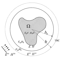
Figure 1.1: An illustration of the geometry

One of the main purposes of this paper is devoted to deriving new formulas of the NRBC by using the compact VSH expansion of the scattering field. For the convolution kernel in the NRBC, an explicit expression in time domain is obtained based on a direct inversion of the Laplace transform (see Theorem 2.2 below). As shown in [3, 40], the explicit expressions of NRBKs allow for a rapid and accurate evaluation of the convolution in NRBC.

The second main purpose of this paper is to propose an accurate and efficient numerical method for the simulation of the electromagnetic invisibility cloaks by using the new NRBC formula and the compact VSH expansion. Transformation optics originated from the seminal works [33, 18] offers an effective approach to design novel and unusual optical devices such as the invisibility cloaks (see, e.g., [33, 9]), superlens (see, e.g., [42, 39]) and beam splitters (see, e.g., [34]), etc. Numerical simulation plays a crucial role in modelling of the electromagnetic wave interaction with these devices since it serves as a reliable tool to the justification of expensive physical experiments and validation of theoretical predictions. Over the recent years, intensive simulations and analysis have been devoted to the frequency domain (see, e.g., [7, 35, 46, 47, 25, 17, 44, 45]). Due to the fact that metamaterials used for manufacturing such kind of devices are unavoidably dispersive (cf. [32]), i.e., $\bm{\varepsilon}$ and $\bm{\mu}$ are frequency-dependent, time-domain mathematical models and simulations of anisotropic and dispersive electromagnetic devices are of fundamental importance. However, only limited works are available for the time-domain simulations including the FDTD [48, 49, 29] and the FETD [19, 21, 22, 43, 24]. Because of the computational complexity, so far the numerical simulation of spherical cloaking structures has only been examined by [49] with a parallel implementation of FDTD method. In this paper, we propose a new formulation of the spherical cloak model in the time domain using the Drude dispersion model (cf. [31]). This new formulation allows us to use the symmetry of the problem together with the compact VSH expansions to provide an efficient VSH-spectral-element method for the simulation. Compared with the classic FDTD based algorithm, the VSH-spectral-element method can produce accurate numerical results in much less computational cost.

The rest of the paper is organised as follows. In section 2, we present some new formulas of the NRBC and derive an explicit expression for the underlying convolution kernel. In section 3, we first derive a new time-domain model for the spherical dispersive cloaks by using Drude model. Then, an VSH-spectral-element method with Newmark’s time integration scheme is proposed for efficient simulation of spherical cloaks. Ample interesting simulations for the spherical dispersive cloaks are presented in section 4 to show the accuracy and efficiency of the proposed numerical scheme.

2 Computation of time-domain NRBC

In this section, we present the formulations of the capacity operator ${\mathscr{T}}_{b}$ involved in the time-domain NRBC, and then derive some analytically perspicuous formulas for the associated temporal convolution kernels (dubbed as NRBKs), which are crucial for efficient and accurate computation of the NRBC, and in return for its seamless integration with the interior solvers.

2.1 Formulation of time-domain NRBC

Let $L^{2}(\Omega)$ be the usual space of square integrable functions on $\Omega,$ and denote $\bm{L}^{2}(\Omega)=(L^{2}(\Omega))^{3}.$ We introduce the spaces

$$\begin{split}{\mathbb{H}}({\rm div};\Omega)=\big{\{}\bm{v}\in{\bm{L}}^{2}(\Omega):{\rm div}\bm{v}\in L^{2}(\Omega)\big{\}};\;\;{\mathbb{H}}({\bf curl};\Omega)=\big{\{}\bm{v}\in(L^{2}(\Omega))^{3}:\nabla\times{\bm{v}}\in{\bm{L}}^{2}(\Omega)\big{\}},\end{split}$$

which are equipped with the graph norms as defined in [26, p. 52]. We further define

$${\mathbb{H}}_{0}({\rm div};\Omega)=\big{\{}\bm{v}\in{\mathbb{H}}({\rm div};\Omega):{\rm div}\bm{v}=0\big{\}}.\;$$

For $0\not=\bm{x}\in\mathbb{R}^{3},$ let ${\bm{e}}_{r}=\bm{x}/|\bm{x}|.$ Recall that the VSH

$$\big{\{}\bm{Y}_{l}^{m},\bm{\Psi}_{l}^{m},\bm{\Phi}_{l}^{m}\big{\}}:=\big{\{}Y_{l}^{m}{\bm{e}}_{r},\nabla_{S}Y_{l}^{m},\nabla_{S}Y_{l}^{m}\times{\bm{e}}_{r}\big{\}}$$ (2.1)

used in the Spherepack [37] forms a complete orthogonal basis of ${\bm{L}}^{2}(S):=(L^{2}(S))^{3},$ where $\{Y_{l}^{m}\}$ are the spherical harmonic basis defined on the unit sphere $S$ as in [28]. Nevertheless, the following compact form of the VSH expansion of a solenoidal or divergence-free field in (2.2) can simplify the derivation of NRBC. Moreover, it will lead to more efficient spectral-element algorithm for the 3D spherical cloaking simulation in Section 3.

Proposition 2.1.

For $\bm{u}\in{\mathbb{H}}_{0}({\rm div};\Omega)$, we can write

$${\bm{u}}=u_{00}\,\bm{Y}_{0}^{0}+\sum_{l=1}^{\infty}\sum_{|m|=0}^{l}\Big{\{}u_{lm}\,{\bm{\Phi}}_{l}^{m}+\nabla\times\big{(}\tilde{u}_{lm}\,{\bm{\Phi}}_{l}^{m}\big{)}\Big{\}},$$ (2.2)

where $u_{00}$ satisfies

$$\Big{(}\frac{d}{dr}+\frac{2}{r}\Big{)}u_{00}=0\;\;\;{\rm or}\;\;\;u_{00}=\frac{C}{r^{2}},$$ (2.3)

for a constant $C$ depends on the average value of the $\bm{e}_{r}$ component of $\bm{u}$ on $S$. The expansion (2.2) can be reformulated in terms of the VSH (2.1) as follows

$${\bm{u}}=u_{00}\,\bm{Y}_{0}^{0}+\sum_{l=1}^{\infty}\sum_{|m|=0}^{l}\Big{\{}\frac{\beta_{l}}{r}\tilde{u}_{lm}\,\bm{Y}_{l}^{m}+\hat{\partial}_{r}\tilde{u}_{lm}\,\bm{\Psi}_{l}^{m}+u_{lm}\,{\bm{\Phi}}_{l}^{m}\Big{\}},$$ (2.4)

where $\beta_{l}:=l(l+1)$ and

$$\begin{split}&u_{lm}(r)={\beta_{l}^{-1}}\big{\langle}\bm{u},{\bm{\Phi}}_{l}^{m}\big{\rangle}_{S},\quad r^{-1}\tilde{u}_{lm}(r)=\beta_{l}^{-1}\big{\langle}\bm{u},\bm{Y}_{l}^{m}\big{\rangle}_{S}.\end{split}$$ (2.5)

Proof.

We first show that if (2.3) holds, then the expansion (2.2) automatically satisfies ${\rm div}\,\bm{u}=0.$ Note that ${\rm div}(u_{lm}\,{\bm{\Phi}}_{l}^{m})=0$ (cf. (A.9)). Performing the divergence operator on (2.2), and using (A.11), we have ${\rm div}\,\bm{u}=0,$ if $u_{00}$ satisfies the equation in (2.3) which has explicit solution: $u_{00}=C/r^{2}$. Thanks to (A.10), the expansion (2.4) follows immediately from (2.2). Then (2.5) is a direct consequence of the orthogonality of VSH. ∎

Remark 2.1.

For any constant $C,$ the field $C\,{\bm{e}}_{r}/r^{2},r>0$ (note: $Y_{0}^{0}=1/{(2\sqrt{\pi})}$) is solenoidal. Given a vector field, the VSH expansion coefficients in (2.5) can be evaluated accurately and efficiently by using discrete VSH-transforms in SpherePack [37]. ∎

The time-domain NRBC to be formulated below involves the modified spherical Bessel function (cf. [41]) defined by

$$k_{l}(z)=\sqrt{\frac{\pi}{2z}}K_{l+1/2}(z),$$ (2.6)

with $K_{l+1/2}(\cdot)$ being the modified Bessel function of the second kind of order $l+1/2$, together with the temporal convolution and inverse Laplace transform:

$$(f\ast g)(t)=\int_{0}^{t}f(\tau)g(t-\tau)d\tau,\quad{\mathscr{L}}^{-1}[F](t)=\frac{1}{2\pi{\rm i}}\int_{\gamma-\infty{\rm i}}^{\gamma+\infty{\rm i}}F(s)e^{st}ds,$$

where $F(s)$ is the Laplace transform of $f(t),$ and the integration is done along the vertical line $\Re(s)=\gamma$ in the complex plane such that $\gamma$ is greater than the real part of all singularities of $F(s)$.

The formulation of the capacity operator can be found in e.g., [6, 28, 26], but the notation and normalisation are very different. Here, we feel compelled to sketch its derivation.

Theorem 2.1.

The time-domain capacity operator $\mathscr{T}_{b}$ takes the form

$${\mathscr{T}}_{b}[\bm{E}^{\rm sc}]:=\frac{c}{b}\sum_{l=1}^{\infty}\sum_{m=-l}^{l}\Big{\{}\big{(}\rho_{l}\ast{\psi}^{(1)}_{lm}\big{)}\,{\bm{\Psi}}_{l}^{m}+\big{(}\sigma_{l}\ast{\psi}^{(2)}_{lm}\big{)}\,{\bm{\Phi}}_{l}^{m}\Big{\}},$$ (2.7)

where the convolution kernels are given by the inverse Laplace transforms:

$$\begin{split}\rho_{l}(t)&={\mathscr{L}}^{-1}\bigg{[}z\,\bigg{(}\frac{z\,k_{l}(z)}{k_{l}(z)+z\,k_{l}^{\prime}(z)}+1\bigg{)}\bigg{]}(t),\quad\sigma_{l}(t)={\mathscr{L}}^{-1}\bigg{[}1+z+z\frac{k_{l}^{\prime}(z)}{k_{l}(z)}\bigg{]}(t),\end{split}$$ (2.8)

with $z=\frac{sb}{c}$, and where $\{{\psi}^{r}_{lm},{\psi}^{(1)}_{lm},{\psi}^{(2)}_{lm}\}$ are the VSH expansion coefficients of $\bm{E}^{\rm sc}$ at the spherical surface $r=b$, i.e.,

$$\bm{E}^{\rm sc}=\psi_{00}\,\bm{Y}_{0}^{0}+\sum_{l=1}^{\infty}\sum_{|m|=0}^{l}\Big{\{}{\psi}^{r}_{lm}\,\bm{Y}_{l}^{m}\,+{\psi}_{lm}^{(1)}\bm{\Psi}_{l}^{m}+{\psi}_{lm}^{(2)}\,{\bm{\Phi}}_{l}^{m}\Big{\}}.$$ (2.9)

Proof.

Consider the Maxwell’s equations exterior to the artificial ball $B:=\{\bm{r}:|\bm{r}|<b\}:$

$$\varepsilon_{0}\partial_{t}\bm{E}^{\rm e}-\nabla\times\bm{H}^{\rm e}=\bm{0},\quad\mu_{0}{\partial_{t}\bm{H}}^{\rm e}+\nabla\times\bm{E}^{\rm e}=\bm{0},\;\;{\rm in}\;\;{\mathbb{R}}^{3}\setminus\bar{B},\;\;t>0,$$ (2.10a)

$${\bm{E}}^{\rm e}\times\hat{\bm{r}}=\bm{\lambda},\quad r=b,\;\;\;t>0$$ (2.10b)

$${\partial_{t}\bm{E}_{T}^{\rm e}}-\eta\,{\partial_{t}\bm{H}^{\rm e}}\times\hat{\bm{r}}=o(r^{-1}),\quad|\bm{r}|\to\infty,\;\;t>0,$$ (2.10c)

$$\bm{E}^{\rm e}=\bm{H}^{\rm e}=\bm{0},\quad{\rm in}\;\;{\mathbb{R}}^{3}\setminus\bar{B},\;\;\;t=0,$$ (2.10d)

where $\bm{\lambda}$ is a given field. It is known that this system can be solved analytically by using Laplace transform in time and separation of variables in space. For this purpose, we denote by $\breve{\bm{E}}^{\rm e},\breve{\bm{H}}^{\rm e}$ and $\breve{\bm{\lambda}}$ the Laplace transforms of $\bm{E}^{\rm e},\bm{H}^{\rm e}$ and ${\bm{\lambda}}$ with respect to $t$, respectively. As $\breve{\bm{E}}^{\rm e}$ is a divergence-free vector field, we have from Proposition 2.1 that

$$\breve{\bm{E}}^{\rm e}=\breve{u}_{00}\bm{Y}_{0}^{0}+\sum_{l=1}^{\infty}\sum_{|m|=1}^{l}\big{\{}\breve{u}_{lm}\bm{\Phi}_{l}^{m}+\nabla\times\big{(}\breve{v}_{lm}\bm{\Phi}_{l}^{m}\big{)}\big{\}}.$$ (2.11)

According to [28, Chap. ​​5], the Laplace transformed system of (2.10) in $s$-domain

$$\varepsilon_{0}s\breve{\bm{E}}^{\rm e}-\nabla\times\breve{\bm{H}}^{\rm e}=\bm{0},\quad\mu_{0}s\breve{\bm{H}}^{\rm e}+\nabla\times\breve{\bm{E}}^{\rm e}=\bm{0};\quad\breve{\bm{E}}^{\rm e}\times\hat{\bm{r}}=\breve{\bm{\lambda}}\;\;{\rm at}\;\;r=b,$$ (2.12)

has the exact solution (2.11) with $\breve{u}_{00}=0$ and

$$\breve{u}_{lm}(r)=-\frac{k_{l}(sr/c)}{k_{l}(sb/c)}\breve{\lambda}_{lm}^{(1)},\quad\breve{v}_{lm}=\frac{k_{l}(sr/c)}{\hat{\partial}_{r}k_{l}(sb/c)}\breve{\lambda}_{lm}^{(2)},\quad l\geq 1,$$ (2.13)

where $\hat{\partial}_{r}=\frac{d}{dr}+\frac{1}{r}$, $\{\breve{\lambda}_{lm}^{(1)},\breve{\lambda}_{lm}^{(2)}\}$ are the VSH expansion coefficients of $\breve{\bm{\lambda}}$ (involving only the tangential components). Moreover, we can derive the electric-to-magnetic Calderon (EtMC) operator that maps the data $\breve{\bm{\lambda}}$ to $\breve{\bm{H}}^{\rm e}\times\hat{\bm{r}}$ (cf. [6, 26]) as follows

$$\breve{\bm{H}}^{\rm e}\times\hat{\bm{r}}=-\frac{1}{s\mu_{0}}\sum_{l=1}^{\infty}\sum_{m=-l}^{l}\bigg{\{}\frac{s^{2}k_{l}(sr/c)}{c^{2}\hat{\partial}_{r}k_{l}(sb/c)}\breve{\lambda}_{lm}^{(2)}\bm{\Psi}_{l}^{m}-\frac{\hat{\partial}_{r}k_{l}(sr/c)}{k_{l}(sb/c)}\breve{\lambda}_{lm}^{(1)}\bm{\Phi}_{l}^{m}\bigg{\}},$$ (2.14)

which can be derived from the second equation in (2.11) and the properties of VSH in Appendix A. By requiring the scattering fields $\{\breve{\bm{E}}^{\rm sc},\breve{\bm{H}}^{\rm sc}\}$ to be identical to the exterior fields $\{\breve{\bm{E}}^{\rm e},\breve{\bm{H}}^{\rm e}\}$ across the artificial boundary $r=b,$ and setting $\breve{\bm{E}}^{sc}\times\hat{\bm{r}}|_{r=b}=\breve{\bm{\lambda}},$ we obtain

$$\begin{split}\mu_{0}s\breve{\bm{H}}^{\rm sc}\times\hat{\bm{r}}\big{|}_{r=b}&=-\sum_{l=1}^{\infty}\sum_{m=-l}^{l}\Big{\{}\frac{s^{2}k_{l}(sb/c)}{c^{2}\hat{\partial}_{r}k_{l}(sb/c)}\breve{\psi}^{(1)}_{lm}\bm{\Psi}_{l}^{m}+\frac{\hat{\partial}_{r}k_{l}(sb/c)}{k_{l}(sb/c)}\breve{\psi}^{(2)}_{lm}\bm{\Phi}_{l}^{m}\Big{\}}\\ &=-\sum_{l=1}^{\infty}\sum_{m=-l}^{l}\Big{\{}\Big{(}\frac{1}{b}\mathscr{L}[\rho_{l}]-\frac{s}{c}\Big{)}\breve{\psi}^{(1)}_{lm}\bm{\Psi}_{l}^{m}+\Big{(}\frac{1}{b}\mathscr{L}[\sigma_{l}]-\frac{s}{c}\Big{)}\breve{\psi}^{(2)}_{lm}\bm{\Phi}_{l}^{m}\Big{\}}\\ &=-\frac{1}{b}\sum_{l=1}^{\infty}\sum_{m=-l}^{l}\Big{\{}\mathscr{L}[\rho_{l}]\breve{\psi}^{(1)}_{lm}\bm{\Psi}_{l}^{m}+\mathscr{L}[\sigma_{l}]\breve{\psi}^{(2)}_{lm}\bm{\Phi}_{l}^{m}\Big{\}}+\frac{s}{c}\breve{\bm{E}}_{T}^{\rm sc},\end{split}$$ (2.15)

where $\sigma_{l}(t)$ and $\rho_{l}(t)$ are defined in (2.8). Transforming the relation (2.15) back to $t$-domain leads to the time-domain NRBC

$$\partial_{t}{\bm{E}}^{\rm sc}_{T}-\eta\partial_{t}\bm{H}^{\rm sc}\times\hat{\bm{r}}-\mathscr{T}_{b}[{\bm{E}}^{\rm sc}]=\bm{0}\quad{\rm at}\;\;\;r=b,$$ (2.16)

and the capacity operator ${\mathscr{T}}_{b}[\bm{E}^{\rm sc}]$ given by (2.7). ∎

Remark 2.2.

Note that the exact NRBC in [13] expressed as a system of $\bm{E}^{\rm sc}$ and $\bm{H}^{\rm sc}$, is actually equivalent to the formulation (1.6d) by using the VSH $\big{\{}\bm{Y}_{l}^{m},\bm{\Psi}_{l}^{m},\bm{\Phi}_{l}^{m}\big{\}}$. From the NRBC (1.6d) on scattering fields, the NRBC (1.5c) on total field $\{\bm{E},\bm{H}\}$ can be derived straightforwardly as follows

$$\partial_{t}{\bm{E}}_{T}-\eta\partial_{t}\bm{H}\times\hat{\bm{r}}-\mathscr{T}_{b}[{\bm{E}}]=\partial_{t}{\bm{E}}_{T}^{\rm in}-\eta\partial_{t}\bm{H}^{\rm in}\times\hat{\bm{r}}-\mathscr{T}_{b}[{\bm{E}}^{\rm in}]:=\bm{h},\quad{\rm at}\;\;\;r=b.$$ (2.17)

We shall see from (2.7) and (2.17) that the source term $\bm{h}$ needs to be precomputed from $\{\bm{E}^{\rm in},\bm{H}^{\rm in}\}$ if the model (1.5) is used for solving the total field $\{\bm{E},\bm{H}\}$ in the whole computational domain $B$. However, the involved term $\mathscr{T}_{b}[{\bm{E}}^{\rm in}]$ is computationally costly due to: (i) The VSH expansion coefficients of the incident wave are necessary for the computation; (ii) in the time direction, two convolutions need to be calculated numerically for each group of VSH expansion coefficients; (iii) the numerical scheme for the convolution needs to be more accurate than the time discretization scheme for the model problem due to sensitivity of the operator $\mathscr{T}_{b}$ on the error. Thus, a great number of time consuming VSH expansion need to be performed. ∎

It is seen from (2.7) that to compute ${\mathscr{T}}_{b}[\bm{E}^{\rm sc}]$ at $t>0,$ it requires

• accurate evaluation of the convolution kernel functions: $\rho_{l}(t)$ and $\sigma_{l}(t)$ defined in (2.8);

• fast computation of the temporal convolutions: $\rho_{l}\ast{\psi}^{(1)}_{lm}$ and $\sigma_{l}\ast{\psi}^{(2)}_{lm}.$

With these, we can compute ${\mathscr{T}}_{b}[\bm{E}^{\rm sc}]$ on the sphere $r=b$ by using the VSH transform in the Spherepack [37].

We now deal with the first issue. Interestingly, the kernel function $\sigma_{l}(t)$ coincides with the NRBC kernel of the transient wave equation, which admits the following explicit formula (cf. [36, 13, 40]).

Proposition 2.2.

Let $\sigma_{l}(t)$ be the kernel function defined in (2.8). Then we have

$$\sigma_{l}(t)=\frac{c}{b}\sum_{j=1}^{l}z_{j}^{l}e^{\frac{c}{b}z_{j}^{l}t},\quad l\geq 1,\;\;t\geq 0,$$ (2.18)

where $\{z_{j}^{l}\}_{j=1}^{l}$ are the zeros of $K_{l+1/2}(z)$ with $l\geq 1$.

We remark that according to [41, p. 511], $K_{l+1/2}(z)$ has exactly $l$ zeros in conjugate pairs which are simple and lie in the second and third quadrants. The interested readers might refer to [40, Lemma 2.1] for more details.

Remarkably, we can derive a very similar analytical formula for the kernel function $\rho_{l}(t).$ Our starting point is to rewrite the ratio of the modified Bessel functions in (2.8) by using (2.6) as follows

$$\begin{split}&z\bigg{(}\frac{zk_{l}(z)}{k_{l}(z)+zk^{\prime}_{l}(z)}+1\bigg{)}=z\bigg{(}\frac{zK_{l+1/2}(z)}{\frac{1}{2}K_{l+1/2}(z)+zK^{\prime}_{l+1/2}(z)}+1\bigg{)}.\end{split}$$ (2.19)

We are interested in the poles of the ratio, i.e., zeros of $\frac{1}{2}K_{l+1/2}(z)+zK^{\prime}_{l+1/2}(z)$. It is indeed very fortunate to find the following results in [38, Lemmas 1-2] (for more general combination of this form).

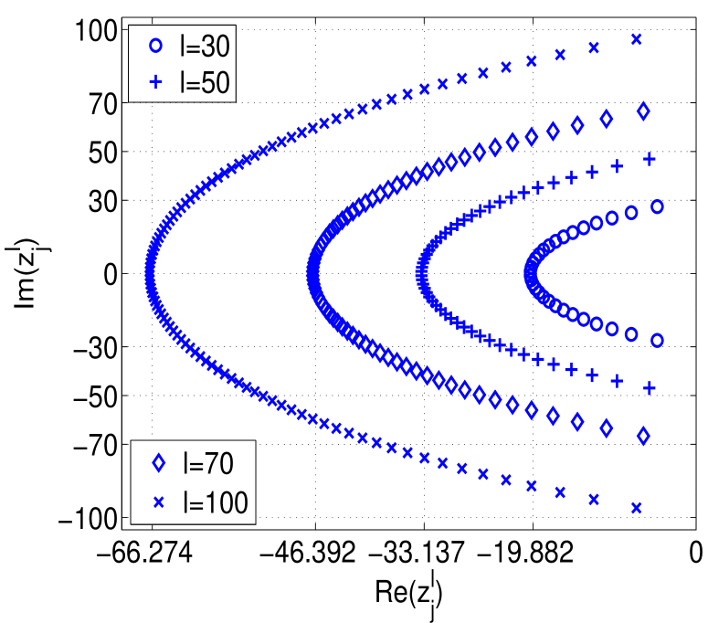
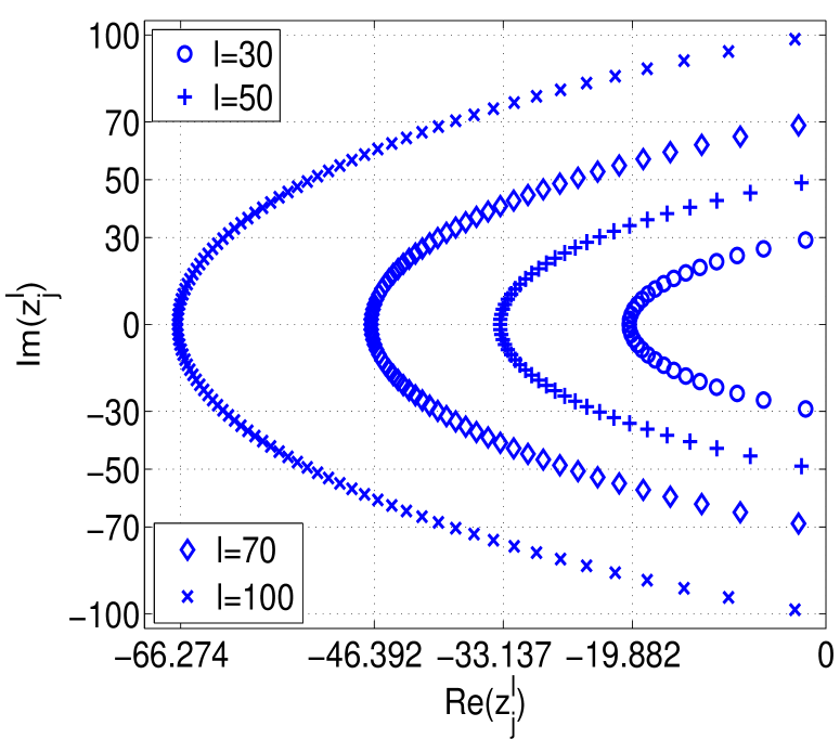
Figure 2.1: Distributions of the zeros of $K_{l+1/2}(z)$ (left) and $\frac{1}{2}K_{l+1/2}(z)+zK^{\prime}_{l+1/2}(z)$ (right).

Lemma 2.1.

Let $l$ be a nonnegative integer. Then we have the following properties.

• $\frac{1}{2}K_{l+1/2}(z)+zK^{\prime}_{l+1/2}(z)$ has exactly $l+1$ zeros.

• If $z_{*}$ is a zero of $\frac{1}{2}K_{l+1/2}(z)+zK^{\prime}_{l+1/2}(z)$, then its complex conjugate $\bar{z}_{*}$ is also a zero.

• All zeros of $\frac{1}{2}K_{l+1/2}(z)+zK^{\prime}_{l+1/2}(z)$ are simple and have negative real parts, so they lie in the left half of the complex plane.

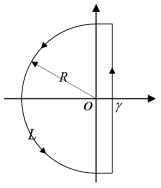
Figure 2.2: Contour $L$ for the inverse Laplace transform.

We illustrate in Figure 2.1 the distribution of zeros of $K_{l+1/2}(z)$ (left) and $\frac{1}{2}K_{l+1/2}(z)+zK^{\prime}_{l+1/2}(z)$ (right) for various $l.$ We observe that for a given $l$, the zeros of $\frac{1}{2}K_{l+1/2}(z)+zK^{\prime}_{l+1/2}(z)$ have a distribution very similar to those of $K_{l+1/2}(z)$, that is, sitting on the left half boundary of an eye-shaped domain that intersects the imaginary axis approximately at $\pm l{\rm i},$ and the negative real axis at $-la$ with $a\approx 0.66274$ (see the vertical dashed coordinate grids). Such a behaviour is very similar to that of $K_{l+1/2}(z)$ (cf. [40]).

With the above understanding, we now ready to present the analytical formula for the convolution kernel function $\rho_{l}(t)$.

Theorem 2.2.

Let $\{\tilde{z}_{j}^{l}\}_{j=1}^{l+1}$ be the zeros of $\frac{1}{2}K_{l+1/2}(z)+zK^{\prime}_{l+1/2}(z)$ with integer $l\geq 0$. Then we can compute $\rho_{l}(t)$ in (2.8) via

$$\begin{split}\rho_{l}(t)&=\frac{c}{b}\sum_{j=1}^{l+1}\frac{(\tilde{z}_{j}^{l})^{3}}{l(l+1)+(\tilde{z}_{j}^{l})^{2}}\,e^{ct\tilde{z}_{j}^{l}/b}+\delta(t)\sum_{j=1}^{l+1}\frac{(\tilde{z}_{j}^{l})^{2}}{l(l+1)+(\tilde{z}_{j}^{l})^{2}},\end{split}$$ (2.20)

where $\delta(t)$ is the Dirac delta function.

Proof.

Using the property

$$\mathscr{L}^{-1}[sf(s)](t)=f^{\prime}(t)+f(0)\delta(t),$$ (2.21)

we obtain from (2.8) and (2.19) that

$$\rho_{l}(t)=\mathscr{L}^{-1}\bigg{[}z\,\bigg{(}\frac{z\,k_{l}(z)}{k_{l}(z)+z\,k_{l}^{\prime}(z)}+1\bigg{)}\bigg{]}(t)=\frac{b}{c}\big{(}\tilde{\rho}^{\prime}_{l}(t)+\tilde{\rho}_{l}(0)\delta(t)\big{)},$$ (2.22)

where $z={sb}/{c},$ and with a change of variable $s=cz/b,$ we have

$$\begin{split}\tilde{\rho}_{l}(t)&=\frac{1}{2\pi{\rm i}}\frac{c}{b}\int_{\gamma-\infty{\rm i}}^{\gamma+\infty{\rm i}}\bigg{[}\frac{zk_{l}(z)}{k_{l}(z)+zk^{\prime}_{l}(z)}+1\bigg{]}e^{czt/b}dz:=\frac{1}{2\pi{\rm i}}\frac{c}{b}\int_{\gamma-\infty{\rm i}}^{\gamma+\infty{\rm i}}F_{l}(z)e^{czt/b}dz.\end{split}$$ (2.23)

In view of the formula (see [30, 10.49.12]):

$$k_{l}(z)=\frac{\pi}{2}\sum\limits_{k=0}^{l}\frac{(l+k)!e^{-z}}{2^{k}k!(l-k)!z^{k+1}},\quad l\geq 0,$$ (2.24)

and Lemma 2.1, we conclude that $F_{l}(z)$ is a meromorphic function. We introduce the closed contour $L$ as depicted in Figure 2.2. Using the residue theorem and Jordan’s Lemma, we have

$$2\pi{\rm i}\sum\limits_{j=1}^{l+1}{\rm Res}\,\big{[}F_{l}(z)e^{czt/b};\tilde{z}_{j}^{l}\big{]}=\lim_{R\to+\infty}\oint_{L}F_{l}(z)e^{czt/b}dz=\int_{\gamma-\infty{\rm i}}^{\gamma+\infty{\rm i}}F_{l}(z)e^{czt/b}dz.$$

From (2.6), we calculate that

$$\begin{split}\frac{b}{c}\tilde{\rho}_{l}(t)&=\sum\limits_{j=1}^{l+1}{\rm Res}\,\big{[}F_{l}(z)e^{czt/b};\tilde{z}_{j}^{l}\big{]}\\ &=\sum\limits_{j=1}^{l+1}\lim_{z\rightarrow\tilde{z}_{j}^{l}}\bigg{\{}\big{(}z-\tilde{z}_{j}^{l}\big{)}e^{ctz/b}\bigg{[}\frac{zK_{l+1/2}(z)}{\frac{1}{2}K_{l+1/2}(z)+zK^{\prime}_{l+1/2}(z)}+1\bigg{]}\bigg{\}}\\ &=\sum\limits_{j=1}^{l+1}\frac{e^{ct\tilde{z}_{j}^{l}/b}\tilde{z}_{j}^{l}K_{l+1/2}(\tilde{z}_{j}^{l})}{\frac{3}{2}K^{\prime}_{l+1/2}(\tilde{z}_{j}^{l})+\tilde{z}_{j}^{l}K^{\prime\prime}_{l+1/2}(\tilde{z}_{j}^{l})}.\end{split}$$ (2.25)

Since $K_{l+1/2}(z)$ satisfies the equation (cf. [41])

$$z^{2}\frac{d^{2}w}{dz^{2}}+z\frac{dw}{dz}-\Big{(}z^{2}+(l+1/2)^{2}\Big{)}w=0,$$

we have

$$\begin{split}z^{2}K^{\prime\prime}_{l+1/2}(z)+\frac{3}{2}zK^{\prime}_{l+1/2}(z)&=\big{(}z^{2}+(l+1/2)^{2}\big{)}K_{l+1/2}(z)-zK^{\prime}_{l+1/2}(z)+\frac{3}{2}zK^{\prime}_{l+1/2}(z)\\ &=\big{(}z^{2}+l(l+1)\big{)}K_{l+1/2}(z)+\frac{1}{2}\bigg{(}\frac{1}{2}K_{l+1/2}(z)+zK^{\prime}_{l+1/2}(z)\bigg{)}.\end{split}$$

A combination of (2.25) and the fact that $\{\tilde{z}_{j}^{l}\}_{j=1}^{l+1}$ are zeros of $\frac{1}{2}K_{l+1/2}(z)+zK^{\prime}_{l+1/2}(z)$ yields

$$\begin{split}\tilde{\rho}_{l}(t)&=\frac{c}{b}\sum\limits_{j=1}^{l+1}\frac{e^{ct\tilde{z}_{j}^{l}/b}\big{(}\tilde{z}_{j}^{l}\big{)}^{2}K_{l+1/2}(\tilde{z}_{j}^{l})}{\big{[}\big{(}\tilde{z}_{j}^{l}\big{)}^{2}+l(l+1)\big{]}K_{l+1/2}(\tilde{z}_{j}^{l})}=\frac{c}{b}\sum\limits_{j=1}^{l+1}\frac{e^{ct\tilde{z}_{j}^{l}/b}\big{(}\tilde{z}_{j}^{l}\big{)}^{2}}{\big{(}\tilde{z}_{j}^{l}\big{)}^{2}+l(l+1)}.\end{split}$$ (2.26)

Inserting (2.26) into (2.22) leads to the expression of $\rho_{l}(t)$ in (2.20). ∎

Having addressed the first issue on how to compute the convolution kernel functions, we now introduce an efficient technique to alleviate the historical burden of temporal convolutions involved in the capacity operator (2.7). Observe from (2.18) and (2.20) that the time variable $t$ only presents in the complex exponentials. As a result, the temporal convolutions can be evaluated recursively as shown in e.g., [3, 40]. More precisely, given a continuous function $g(t)$, we define

$$f(t;z):=e^{ctz/b}\ast g(t)=\int_{0}^{t}e^{c(t-\tau)z/b}g(\tau)d\tau.$$ (2.27)

Then by (2.18) and (2.20),

$$(\sigma_{l}\ast g)(t) =\frac{c}{b}\sum_{j=1}^{l}z_{j}^{l}f(t;z_{j}^{l});$$ (2.28a)

$$(\rho_{l}\ast g)(t) =\frac{c}{b}\sum_{j=1}^{l+1}\frac{\big{(}\tilde{z}_{j}^{l}\big{)}^{3}f(t;\tilde{z}_{j}^{l})}{\big{(}\tilde{z}_{j}^{l}\big{)}^{2}+l(l+1)}+g(t)\sum_{j=1}^{l+1}\frac{\big{(}\tilde{z}_{j}^{l}\big{)}^{2}}{\big{(}\tilde{z}_{j}^{l}\big{)}^{2}+l(l+1)}.$$ (2.28b)

One verifies readily that

$$f(t+\Delta t;z)=e^{c\Delta t\,z/b}f(t;z)+\int_{t}^{t+\Delta t}e^{c(t+\Delta t-\tau)z/b}g(\tau)\,d\tau,$$ (2.29)

so $f(t;z)$ can march in $t$ with step size $\Delta t$ recursively. As a result, the temporal convolution in the NRBC can be computed efficiently with the explicit expressions (2.18) and (2.20), and with the above fast recursive algorithm.

Next, we provide some numerical results to demonstrate the high accuracy in computing $\rho_{l}(t)$ and the related convolution in (2.20). Let $\phi(t),t\geq 0$ be a given differentiable function such that $\phi(0)=0.$ As shown in [40], $(\sigma_{l}\ast\phi)(t)$ can be computed very accurately (i.e., using Proposition 2.2 and (2.28a)). Let $\psi_{l}(t)$ be a function associated with $\phi(t)$ through

$$\mathscr{L}[\psi_{l}](s)=\frac{k_{l}(z)+zk^{\prime}_{l}(z)}{k_{l}(z)}\mathscr{L}[\phi](s)=\left(\!1+z+z\frac{k^{\prime}_{l}(z)}{k_{l}(z)}\right)\!\mathscr{L}[\phi](s)-z\mathscr{L}[\phi](s),$$ (2.30)

where $z=sb/c.$ Applying the inverse Laplace transform and using the definition of $\sigma_{l}(t)$ in (2.8), we obtain from (2.21), $\phi(0)=0$ and Proposition 2.2 that

$$\psi_{l}(t)=(\sigma_{l}\ast\phi)(t)-\frac{b}{c}\phi^{\prime}(t)=\frac{c}{b}\sum_{j=1}^{l}(z_{j}^{l})^{2}e^{ctz_{j}^{l}/b}\ast\phi(t)+\phi(t)\sum_{j=1}^{l}z_{j}^{l}.$$ (2.31)

We next present two ways to compute $(\rho_{l}\ast\psi_{l})(t),$ where the first one only requires the use of the formula for $\sigma_{l}(t).$ Indeed, we have from (2.8), (2.21) and (2.30) that

$$\begin{split}(\rho_{l}\ast\psi_{l})(t)&=\mathscr{L}^{-1}\bigg{[}z\Big{(}\frac{z\,k_{l}(z)}{k_{l}(z)+z\,k_{l}^{\prime}(z)}+1\Big{)}\mathscr{L}[\psi_{l}]\bigg{]}=\mathscr{L}^{-1}\big{[}z^{2}\mathscr{L}[\phi]+z\mathscr{L}[\psi_{l}]\big{]}\\ &=\mathscr{L}^{-1}\bigg{[}\Big{(}1+z+z\frac{k^{\prime}_{l}(z)}{k_{l}(z)}\Big{)}z\mathscr{L}[\phi]\bigg{]}=\sigma_{l}\ast\mathscr{L}^{-1}\big{[}z\mathscr{L}[\phi]\big{]}=(\sigma_{l}\ast\phi^{\prime})(t).\end{split}$$ (2.32)

Then, by Proposition 2.2 and integration by parts, we find

$$\begin{split}(\rho_{l}\ast\psi_{l})(t)&=\sum_{j=1}^{l}z_{j}^{l}e^{ctz_{j}^{l}/b}\ast\phi^{\prime}(t)=\frac{c}{b}\sum_{j=1}^{l}(z_{j}^{l})^{2}e^{ctz_{j}^{l}/b}\ast\phi(t)+\phi(t)\sum_{j=1}^{l}z_{j}^{l}.\end{split}$$ (2.33)

On the other hand, using Theorem 2.2 and the relation (2.31) leads to

$$\begin{split}(\rho_{l}\ast\psi_{l})(t)&=\frac{c}{b}\sum_{j=1}^{l+1}\frac{\big{(}\tilde{z}_{j}^{l}\big{)}^{3}}{\big{(}\tilde{z}_{j}^{l}\big{)}^{2}+l(l+1)}e^{ct\tilde{z}_{j}^{l}/b}\ast\psi_{l}(t)+\psi_{l}(t)\sum_{j=1}^{l+1}\frac{\big{(}\tilde{z}_{j}^{l}\big{)}^{2}}{\big{(}\tilde{z}_{j}^{l}\big{)}^{2}+l(l+1)},\end{split}$$ (2.34)

where $\psi_{l}$ is computed by (2.31). It is evident that the convolutions in (2.33)-(2.34) can be evaluated by using (2.29).

It is seen that (2.33) and (2.34) are equivalent, but the former solely involves $\sigma_{l}(t),$ which can used as a reference to check the accuracy of $\rho_{l}(t).$ We take $b=3,c=5$ and $\phi(t)=\sin^{6}(8t)$, so we can compute the two functions and convolutions with exponential functions in (2.33)-(2.34) exactly. We tabulate in Table 2.1 the relative errors

$$e_{l}(t)=\frac{|f_{l}(t)-\tilde{f}_{l}(t)|}{|\tilde{f}_{l}(t)|},$$

where $f_{l}(t)$ and $\tilde{f}_{l}(t)$ denote the convolution computed by (2.34) and (2.33), respectively. We can see that the relative errors are of machine accuracy, which validate the formula (2.20).

Table 2.1: The relative error $e_{l}(t)$ for different $l$ and $t$.

$l$	$t=1$	$t=2$	$t=4$	$t=10$
1	3.0366e-015	1.9953e-016	2.6091e-015	2.5178e-015
5	2.0593e-015	7.5062e-015	3.8667e-015	1.7176e-014
10	8.2695e-015	1.7839e-014	3.5474e-014	1.5205e-016
15	8.8691e-015	3.5764e-014	1.1748e-014	1.5469e-015
30	4.4403e-015	3.0733e-015	8.0434e-015	2.8513e-015
50	5.0412e-015	3.0602e-015	1.1924e-016	2.9790e-015

Remark 2.3.

It is clear that the number of zeros to be used is determined by the truncation of the expansion (A.6). If $l$ is large, the pole compression algorithm (cf. [2, 16]) can be adopted to obtain approximations for the NRBKs: $\sigma_{l}(t)$ and $\rho_{l}(t)$. The approximated kernels have the same form as in (2.18) and (2.20) while the number of poles in the summation has been reduced significantly.

2.2 An alternative formulation of the capacity operator

It is seen from (2.7) that the capacity operator $\mathscr{T}_{b}[\bm{E}^{\rm sc}]$ only involves the tangential component of the vector field $\bm{E}^{\rm sc}\in{\mathbb{H}}_{0}({\rm div};\Omega).$ In fact, as shown in Proposition 2.1, the VSH expansion coefficients for a divergence-free field satisfy some relation that allows us to derive the following alternative representation of the capacity operator in Theorem 2.1. We find that it has certain advantage in the application in the forthcoming section.

Theorem 2.3.

The time-domain capacity operator ${\mathscr{T}}_{b}$ in Theorem 2.1 can also be formulated as

$${\mathscr{T}}_{b}[\bm{E}^{\rm sc}]=\frac{c}{b}\sum_{l=1}^{\infty}\sum_{|m|=0}^{l}\bigg{\{}\frac{\omega_{l}\ast{\psi}_{lm}^{r}}{l(l+1)}\,{\bm{\Psi}}_{l}^{m}+\big{(}\sigma_{l}\ast{\psi}_{lm}^{(2)}\big{)}\,{\bm{\Phi}}_{l}^{m}\bigg{\}},$$ (2.35)

where $\sigma_{l}$ is given in (2.8) and

$$\begin{split}\omega_{l}(t)=\frac{b}{c}\big{(}\sigma_{l}^{\prime}(t)+\sigma_{l}(0)\delta(t)\big{)}=\frac{c}{b}\sum_{j=1}^{l}\big{(}z_{j}^{l}\big{)}^{2}e^{\frac{c}{b}z_{j}^{l}t}+\delta(t)\sum_{j=1}^{l}z_{j}^{l}.\end{split}$$ (2.36)

Here, the expression (2.35) involves two of the VSH expansion coefficients $\{{\psi}^{r}_{lm},{\psi}^{(1)}_{lm},{\psi}^{(2)}_{lm}\}$ of $\bm{E}^{\rm sc}$ in (2.9).

Proof.

In view of Proposition 2.1, we can reformulate (2.11) as

$$\breve{\bm{E}}^{\rm e}=\breve{u}_{00}\bm{Y}_{0}^{0}+\sum_{l=1}^{\infty}\sum_{|m|=0}^{l}\Big{\{}\breve{u}_{lm}\bm{\Phi}_{l}^{m}+\frac{\beta_{l}}{r}\breve{v}_{lm}\,\bm{Y}_{l}^{m}+\hat{\partial}_{r}\breve{v}_{lm}\,\bm{\Psi}_{l}^{m}\Big{\}},$$ (2.37)

which is a solution of the exterior problem (2.12). Let $\big{\{}\breve{\psi}^{r}_{lm},{\breve{\psi}}^{(1)}_{lm},{\breve{\psi}}^{(2)}_{lm}\big{\}}$ be the Laplace transforms of $\big{\{}{\psi^{r}_{lm},\psi}^{(1)}_{lm},{\psi}^{(2)}_{lm}\big{\}}$, which is the VSH expansion coefficients of the scattering field $\bm{E}^{\rm sc}$ in (2.9). Note that $\breve{\bm{E}}^{\rm e}=\breve{\bm{E}}^{\rm sc}$ is the solution of the exterior problem (2.12) with boundary data $\breve{\bm{\lambda}}=\breve{\bm{E}}^{\rm sc}\times\hat{\bm{r}}$ on the artificial boundary $r=b$. Then by (2.9), (2.13) and (2.37), we arrive at the VSH expansion coefficients of Laplace transformed scattering field $\breve{\bm{E}}^{\rm sc}:$

$$\breve{\psi}^{r}_{lm}=\frac{\beta_{l}}{r}\breve{v}_{lm}=\frac{\beta_{l}}{r}\frac{k_{l}(sr/c)}{\hat{\partial}_{r}k_{l}(sb/c)}\breve{\lambda}_{lm}^{(2)},\quad\breve{\psi}^{(1)}_{lm}=\hat{\partial}_{r}\breve{v}_{lm}=\frac{\hat{\partial}_{r}k_{l}(sr/c)}{\hat{\partial}_{r}k_{l}(sb/c)}\breve{\lambda}_{lm}^{(2)},$$ (2.38)

for $r\geq b$. This implies

$$\breve{\psi}^{r}_{lm}=\frac{\beta_{l}}{r}\frac{k_{l}(sr/c)}{\hat{\partial}_{r}k_{l}(sr/c)}\breve{\psi}^{(1)}_{lm}=\frac{\beta_{l}}{r}\frac{k_{l}(sr/c)}{\frac{s}{c}k_{l}^{\prime}(sr/c)+\frac{1}{r}k_{l}(sr/c)}\breve{\psi}^{(1)}_{lm},$$

so at $r=b,$ we have

$$\frac{\breve{\psi}^{r}_{lm}}{\beta_{l}}=\frac{k_{l}(z)}{k_{l}(z)+z\,k_{l}^{\prime}(z)}\breve{\psi}_{lm}^{(1)},\quad z=\frac{sb}{c}.$$ (2.39)

Multiplying both sides of (2.39) by $(1+z)k_{l}(z)+zk_{l}^{\prime}(z)$ yields

$$z\,\bigg{(}\frac{z\,k_{l}(z)}{k_{l}(z)+z\,k_{l}^{\prime}(z)}+1\bigg{)}\breve{\psi}_{lm}^{(1)}=z\,\bigg{(}1+z+z\frac{k_{l}^{\prime}(z)}{k_{l}(z)}\bigg{)}\frac{\breve{\psi}^{r}_{lm}}{\beta_{l}}.$$ (2.40)

In view of the definitions of $\rho_{l}$ and $\sigma_{l}$ in (2.8) and using the property (2.21), we take the inverse Laplace transform on both sides of (2.40) and find

$$\rho_{l}\ast\psi_{lm}^{(1)}=\frac{\omega_{l}\ast{\psi}_{lm}^{r}}{\beta_{l}},$$ (2.41)

where the kernel function

$$\begin{split}\omega_{l}(t)&={\mathscr{L}}^{-1}\bigg{[}z\,\bigg{(}1+z+z\frac{k_{l}^{\prime}(z)}{k_{l}(z)}\bigg{)}\bigg{]}(t)=\frac{b}{c}\big{(}\sigma_{l}^{\prime}(t)+\sigma_{l}(0)\delta(t)\big{)}.\end{split}$$ (2.42)

Then, substituting (2.41) into (2.7) leads to the capacity operator $\mathscr{T}_{b}[\bm{E}^{sc}]$ in (2.35).

Finally, the last formula in (2.36) can be obtained from (2.2) directly. ∎

3 Simulation of three-dimensional dispersive invisibility cloak

As already mentioned in the introductory section, the invisibility cloak is one of the most appealing examples in the field of transformation optics [33, 10]. In this section, we focus on the time-domain modelling and efficient simulation of the electromagentic invisibility cloak first proposed in [33]. Indeed, there exist very limited works in three-dimensional cloak simulations. Our contributions are twofold. (i) We shall derive a new mathematical formulation of the time-domain dispersive cloak. Different from the existing models based on some mixed forms of both $\bm{E}$ and $\bm{H}$ (see, e.g., [14, 49, 21, 23]), the new formulation only involves one unknown field $\bm{D}$ (see Theorem 3.1), where the seemingly complicated temporal convolutions in the form of (2.27) can be evaluated efficiently as shown in (2.29). Moreover, the proposed governing equation in the cloaking layer with special dispersive media is valid for other geometries (e.g., the polygonal layer) other than the spherical shell. (ii) To simulate the time-domain spherical cloaking designed in [33], we shall develop a very efficient VSH-spectral-element method for solving the reduced problem truncated by the NRBC (2.16) using the alternative formulation of the capacity operator in Theorem 2.3. The implementation of the new algorithm can run thousands of time steps in a few hours on a desktop with intel i7 CPU, while the parallel implementation of the classic FDTD method running on a cluster with 100 processors and 220 GB memory takes 45 hours for 13000 time steps (cf. [49, pp. 7307]).

In this section, we apply the framework (1.6) to the modeling of 3D coordinate transformation based invisibility cloak. The Maxwell’s equations (1.1) is the basic model for cloaking while material parameters $\bm{\varepsilon}$ and $\mu$ in the cloak are designed based on the form invariance of Maxwell equations under coordinate transformations [post1997formal] [33, 10]. For simplicity, we first use the spherical cloak as an example and then generalise the model to other geometrically complicated cloaks. The material parameters of an ideal spherical cloak are given as follows [33]:

$${\bm{\varepsilon}}={\bm{\mu}}={\rm diag}(\epsilon_{r}(r),\epsilon,\epsilon),\quad\epsilon_{r}(r):=\frac{R_{2}}{R_{2}-R_{1}}\Big{(}\frac{r-R_{1}}{r}\Big{)}^{2},\quad\epsilon=\frac{R_{2}}{R_{2}-R_{1}},$$ (3.1)

for $R_{1}<r<R_{2}$, where $R_{1}$ and $R_{2}$ are the inner and outer radii of the cloak, respectively. Because the physical realization of such a kind of cloak must be dispersive [chen2007extending, liang2008], the material parameters in the cloak are frequency dependent. Most of the works [21, 22, 29, 49] on the time domain numerical simulation of cloaking adopt the dispersive modeling proposed in [48]. Here, we derive more compact constitutive relations in time domain and further presented a new model. As in [48], we also use the Drude model to map the material parameters. Nonetheless, we made some manipulations on the form of the constitutive reations in frequency domain and then transform back to time domain to derive a new form. The new form only involves integral operators while the constitutive relations presented in [48] involves both first order and second order derivative operators, see Remark 3.1.

• Write down the mode and present the constiutive relations (like one of Li Jicun’s paper)

• Briefly review the other models to handle the relation (just consider the spherical case. For the general case, we just put a remark)

• Highlight our model, why we formula it in a different model.

3.1 Dispersive modelling of 3D invisibility cloaks

The key to the design of invisibility cloak is to fill the cloaking layer, denoted by $\Omega_{\rm cl}$ (see, e.g., $\Omega_{1}$ in Figure 3.1), with specially designed metamaterials, which can steer electromagnetic waves from penetrating into the enclosed region, and thereby render the interior “invisible” to the outside observer. According to the pioneering work by Pendry et al. [33], the cloaking parameters disperse with frequency and therefore can only be fully effective at a single frequency. To investigate this interesting phenomena, it is necessary to simulate the full wave and consider the non-monochromatic waves passing through such frequency-dependent materials in time domain.

The central issue for time-domain modelling is to formulate the constitutive relations. The material parameters of an ideal spherical cloak are given by (cf. [33]):

$${\bm{\varepsilon}}={\bm{\mu}}={\rm diag}\big{(}\varepsilon(r),\epsilon,\epsilon\big{)},\quad\varepsilon(r)=\frac{R_{2}}{R_{2}-R_{1}}\Big{(}\frac{r-R_{1}}{r}\Big{)}^{2},\quad\epsilon=\frac{R_{2}}{R_{2}-R_{1}},$$ (3.1)

in the cloaking layer $\Omega_{\rm cl}=\{R_{1}<r<R_{2}\}.$ Since $\varepsilon(r)\in[0,1)$, same as in the left-handed materials (LHMs), the material parameters are often mapped by dispersive medium models, e.g., Drude model, Lorentz model [14]. Here, we map $\varepsilon(r)$ (to frequency $\omega$-dependent medium) via the Drude dispersion model:

$$\varepsilon_{k}(r,\omega)=1-\frac{\omega_{p,k}^{2}(r)}{\omega(\omega-{\rm i}\gamma_{k})},\quad\omega_{p,k}(r)=\sqrt{\omega_{c}(\omega_{c}-{\rm i}\gamma_{k})(1-\varepsilon(r))},$$ (3.2)

for $k=1,2,$ leading to the dispersive media in $\Omega_{\rm cl}:$

$$\hat{\bm{\varepsilon}}(r,\omega)={\rm diag}\big{(}\varepsilon_{1}(r,\omega),\epsilon,\epsilon\big{)},\quad\hat{\bm{\mu}}(r,\omega)={\rm diag}\big{(}\varepsilon_{2}(r,\omega),\epsilon,\epsilon\big{)}.$$ (3.3)

In the above expressions, $\omega$ is the wave frequency, $\{\omega_{p,k}\}$ are the plasma frequencies, $\{\gamma_{k}\}$ are damping terms called collision frequencies and $\omega_{c}>0$ is the operating frequency of the cloak. Indeed, if $\omega=\omega_{c},$ then (3.3) reduces to (3.1). Although the ideal lossless case, i.e., $\gamma_{1}=\gamma_{2}=0$ has been adopted in [48, 49, 21], it is physically more reasonable to include the loss effect of the medium in the modeling. Hereafter, we assume that $\gamma_{1}\neq 0,\gamma_{2}\neq 0$.

Denote by $\hat{f}$ the Fourier transform of a generic function $f(t)$, i.e.,

$$\hat{f}(\omega)=\mathscr{F}[f(t)](\omega)=\int_{-\infty}^{+\infty}f(t)e^{-{\rm i}\omega t}dt.$$

Let ${\bm{v}}=(v_{r},v_{\theta},v_{\phi})^{t}$ be a generic vector field, where $v_{r}$, $v_{\theta}$ and $v_{\phi}$ are the components of ${\bm{v}}$ in the coordinate units ${\bm{e}}_{r}$, ${\bm{e}}_{\theta}$ and ${\bm{e}}_{\phi}$, respectively.

Given (3.3), the constitutive relation in the cloaking layer $\Omega_{\rm cl}$ in the frequency domain reads

$$\widehat{\bm{D}}=\big{(}\widehat{D}_{r},\widehat{D}_{\theta},\widehat{D}_{\phi}\big{)}^{t}=\varepsilon_{0}\hat{\bm{\varepsilon}}(r,\omega)\widehat{\bm{E}}=\varepsilon_{0}\big{(}\varepsilon_{1}(r,\omega)\widehat{E}_{r},\epsilon\widehat{E}_{\theta},\epsilon\widehat{E}_{\phi}\big{)}^{t},$$ (3.4)

$$\widehat{\bm{B}}=\big{(}\widehat{B}_{r},\widehat{B}_{\theta},\widehat{B}_{\phi}\big{)}^{t}=\mu_{0}\hat{\bm{\mu}}(r,\omega)\widehat{\bm{H}}=\mu_{0}\big{(}\varepsilon_{2}(r,\omega)\widehat{H}_{r},\epsilon\widehat{H}_{\theta},\epsilon\widehat{H}_{\phi}\big{)}^{t}.$$ (3.5)

Remark 3.1.

The time-domain constitutive equations extensively used in [48, 49, 20, 23] reads

$$\frac{\partial^{2}D_{r}}{\partial t^{2}}+\gamma_{1}\frac{\partial D_{r}}{\partial t}=\varepsilon_{0}\Big{(}\frac{\partial^{2}E_{r}}{\partial t^{2}}+\gamma_{1}\frac{\partial E_{r}}{\partial t}+\omega_{p,1}^{2}E_{r}\Big{)},\quad(D_{\theta},D_{\phi})=\varepsilon_{0}\epsilon(E_{\theta},E_{\phi}),$$ (3.6)

$$\frac{\partial^{2}B_{r}}{\partial t^{2}}+\gamma_{2}\frac{\partial B_{r}}{\partial t}=\mu_{0}\Big{(}\frac{\partial^{2}H_{r}}{\partial t^{2}}+\gamma_{2}\frac{\partial H_{r}}{\partial t}+\omega_{p,2}^{2}H_{r}\Big{)},\quad(B_{\theta},B_{\phi})=\mu_{0}\epsilon(H_{\theta},H_{\phi}),$$ (3.7)

which can be obtained by simply applying the inverse Fourier transform to (3.4)-(3.5). ∎

Different from the existing models, we use (3.4)-(3.5) to derive the following relations in time domain.

Lemma 3.1.

We have the constitutive relations in time domain of the form

$${\bm{E}}=\varepsilon_{0}^{-1}\mathscr{D}_{1}[{\bm{D}}],\quad{\bm{H}}=\mu_{0}^{-1}\mathscr{D}_{2}[{\bm{B}}],$$ (3.8)

where for $k=1,2,$ the operators

$$\mathscr{D}_{k}[\bm{D}]:=\Big{(}D_{r}+\int_{0}^{t}\vartheta_{k}(r,t-\tau)D_{r}(\cdot,\tau)d\tau,\,\epsilon^{-1}D_{\theta},\,\epsilon^{-1}D_{\phi}\Big{)}^{t},$$ (3.9)

with kernel functions given by

$$\vartheta_{k}(r,t)=\frac{{\rm i}\,\omega_{p,k}^{2}(r)}{\zeta^{0}_{k}(r)-\zeta^{1}_{k}(r)}\big{(}e^{{\rm i}\zeta^{0}_{k}(r)t}-e^{{\rm i}\zeta^{1}_{k}(r)t}\big{)}.$$ (3.10)

Here, $\{\zeta^{0}_{k}(r),\zeta^{1}_{k}(r)\}_{k=1}^{2}$ are the roots of the quadratic equation: $z^{2}-{\rm i}\gamma_{k}z-\omega_{p,k}^{2}=0$ given by

$$\begin{split}&\zeta_{k}^{0}(r)=-\frac{1}{\sqrt{2}}\sqrt{\sqrt{\xi_{k}^{2}+\eta_{k}^{2}}+{\xi_{k}}}+{\rm i}\bigg{(}\frac{\gamma_{k}}{2}+\frac{1}{\sqrt{2}}\sqrt{\sqrt{\xi_{k}^{2}+\eta_{k}^{2}}-{\xi_{k}}}\bigg{)},\\ &\zeta_{k}^{1}(r)=\frac{1}{\sqrt{2}}\sqrt{\sqrt{\xi_{k}^{2}+\eta_{k}^{2}}+{\xi_{k}}}+{\rm i}\bigg{(}\frac{\gamma_{k}}{2}-\frac{1}{\sqrt{2}}\sqrt{\sqrt{\xi_{k}^{2}+\eta_{k}^{2}}-{\xi_{k}}}\bigg{)},\end{split}$$ (3.11)

where

$$\xi_{k}=\omega_{c}^{2}\,(1-\varepsilon(r))-\frac{\gamma^{2}_{k}}{4},\quad\eta_{k}=-\gamma_{k}\omega_{c}\,(1-\varepsilon(r)),$$ (3.12)

are the real and imaginary parts of $\omega_{p,k}^{2}-\frac{\gamma^{2}_{k}}{4}$ for $k=1,2.$

Proof.

Using the definition of $\varepsilon_{k}(r,\omega)$ in (3.3), we derive from (3.4)-(3.5) that

$$\widehat{E}_{r}=\varepsilon_{0}^{-1}\Big{(}1+\frac{\omega_{p,1}^{2}(r)}{\omega^{2}-{\rm i}\gamma_{1}\omega-\omega_{p,1}^{2}(r)}\Big{)}\widehat{D}_{r},\quad(\widehat{E}_{\theta},\widehat{E}_{\phi})^{t}=(\varepsilon_{0}\epsilon)^{-1}(\widehat{D}_{\theta},\widehat{D}_{\phi})^{t}\;,$$ (3.13)

$$\widehat{H}_{r}=\mu_{0}^{-1}\Big{(}1+\frac{\omega_{p,2}^{2}(r)}{\omega^{2}-{\rm i}\gamma_{2}\omega-\omega_{p,2}^{2}(r)}\Big{)}\widehat{B}_{r},\quad(\widehat{H}_{\theta},\widehat{H}_{\phi})^{t}=(\mu_{0}\epsilon)^{-1}(\widehat{B}_{\theta},\widehat{B}_{\phi})^{t}.\;$$ (3.14)

Applying the inverse Fourier transform to (3.13)-(3.14) leads to

$$\begin{split}&E_{r}=\varepsilon_{0}^{-1}D_{r}+\varepsilon_{0}^{-1}\omega_{p,1}^{2}(r)\mathscr{F}^{-1}\Big{[}\frac{1}{\omega^{2}-{\rm i}\gamma_{1}\omega-\omega_{p,1}^{2}(r)}\Big{]}\ast D_{r},\;\;\\ &H_{r}=\mu_{0}^{-1}B_{r}+\mu_{0}^{-1}\omega_{p,2}^{2}(r)\mathscr{F}^{-1}\Big{[}\frac{1}{\omega^{2}-{\rm i}\gamma_{2}\omega-\omega_{p,2}^{2}(r)}\Big{]}\ast B_{r},\\[3.0pt] &(E_{\theta},E_{\phi})^{t}=(\varepsilon_{0}\epsilon)^{-1}(D_{\theta},D_{\phi})^{t},\quad(H_{\theta},H_{\phi})^{t}=(\mu_{0}\epsilon)^{-1}(B_{\theta},B_{\phi})^{t},\end{split}$$ (3.15)

where “ $\ast$ ” is the usual convolution as before.

The rest of the derivation is to explicitly evaluate two inverse Fourier transforms. Let $\zeta^{0}_{k},\zeta^{1}_{k}$ be two roots of $z^{2}-{\rm i}\gamma_{k}z-\omega_{p,k}^{2}=0.$ Then we immediately have $\zeta_{k}^{0}+\zeta_{k}^{1}={\rm i}\gamma_{k}$ and $\zeta_{k}^{0}\zeta_{k}^{1}=-\omega_{p,k}^{2},$ so we can write

$$\frac{1}{\omega^{2}-{\rm i}\gamma_{k}\omega-\omega_{p,k}^{2}(r)}=\frac{1}{\zeta_{k}^{0}-\zeta_{k}^{1}}\Big{(}\frac{1}{\omega-\zeta^{0}_{k}}-\frac{1}{\omega-\zeta^{1}_{k}}\Big{)}.$$ (3.16)

Recall that (cf. [4]):

$$\mathscr{F}^{-1}\Big{[}\frac{1}{{\rm i}\omega+a}\Big{]}=-{\rm i}\,\mathscr{F}^{-1}\Big{[}\frac{1}{\omega-a{\rm i}}\Big{]}=e^{-at}H(t),\quad\hbox{if}\;\;\mathfrak{R}\{a\}>0,$$ (3.17)

where $H(t)$ is the Heaviside function. Suppose that we can show

$$\mathfrak{Im}\{\zeta^{0}_{k}\}>0,\quad\mathfrak{Im}\{\zeta^{1}_{k}\}>0.$$ (3.18)

Then by (3.16)-(3.17),

$$\mathscr{F}^{-1}\Big{[}\frac{1}{\omega^{2}-{\rm i}\gamma_{k}\omega-\omega_{p,k}^{2}(r)}\Big{]}=\frac{{\rm i}}{\zeta^{0}_{k}-\zeta^{1}_{k}}\big{(}e^{{\rm i}\zeta^{0}_{k}t}-e^{{\rm i}\zeta^{1}_{k}t}\big{)}H(t).$$ (3.19)

Consequently, we derive (3.9)-(3.10) from (3.15) and (3.19).

It remains to verify (3.11) and (3.18). It is evident that the quadratic equation has the roots:

$$z=\frac{\gamma_{k}}{2}{\rm i}\pm\sqrt{\omega_{p,k}^{2}-\frac{\gamma_{k}^{2}}{4}}=\frac{\gamma_{k}}{2}{\rm i}\pm\sqrt{\xi_{k}+{\rm i}\eta_{k}}\,.$$ (3.20)

Setting $\alpha_{k}+{\rm i}\beta_{k}=\sqrt{\xi_{k}+{\rm i}\eta_{k}}$, we find $\alpha_{k}^{2}-\beta_{k}^{2}=\xi_{k}$ and $2\alpha_{k}\beta_{k}=\eta_{k}.$ Solving this system yields

$$\alpha^{2}_{k}=\frac{\sqrt{\xi_{k}^{2}+\eta_{k}^{2}}+\xi_{k}}{2},\quad\beta^{2}_{k}=\frac{\sqrt{\xi_{k}^{2}+\eta_{k}^{2}}-\xi_{k}}{2}.$$ (3.21)

Noting that $\alpha_{k}\beta_{k}<0,$ we can determine $\alpha_{k},\beta_{k},$ and obtain (3.11) from (3.20). By (3.11), $\mathfrak{Im}\{\zeta^{0}_{k}\}>\mathfrak{Im}\{\zeta^{1}_{k}\},$ so we next show that $\mathfrak{Im}\{\zeta^{1}_{k}\}>0,$ that is,

$$\frac{\gamma_{k}}{2}>\frac{1}{\sqrt{2}}\sqrt{\sqrt{\xi_{k}^{2}+\eta_{k}^{2}}-{\xi_{k}}}\;\;\;{\rm i.e.,}\;\;\;\gamma_{k}^{4}+4\gamma_{k}^{2}\xi_{k}-4\eta_{k}^{2}>0.$$

Direct calculation from (3.12) leads to

$$\gamma_{k}^{4}+4\gamma_{k}^{2}\xi_{k}-4\eta_{k}^{2}=4\gamma_{k}^{2}\omega_{c}^{2}\,\varepsilon(r)\,(1-\varepsilon(r))>0,$$

as $\gamma_{k}\neq 0$, $\omega_{c}>0$ and $0<\varepsilon(r)<1$ (cf. (3.1)). This verifies (3.18) and completes the proof. ∎

With the constitutive relations (3.8)-(3.9) at our disposal, we represent $\bm{E},\bm{H}$ in terms of $\bm{D},\bm{B}$ and then eliminate $\bm{B}$, leading to the following equation in $\Omega_{\rm cl}.$

Theorem 3.1.

Assume that the source term and initial fields vanish in the cloaking layer $\Omega_{\rm cl}$. Then the governing equation in the cloaking layer takes the form

$$\partial^{2}_{t}{\bm{D}}+c^{2}\nabla\times\big{(}\mathscr{D}_{2}[\nabla\times(\mathscr{D}_{1}[{\bm{D}}])]\big{)}=\bm{0}\quad{\rm in}\;\;\Omega_{\rm cl}.$$ (3.22)

Proof.

First, we show that given the homogeneous initial condition $\bm{B}(\bm{r},0)=\bm{0}$, we have $\partial_{t}\mathscr{D}_{2}[\bm{B}]=\mathscr{D}_{2}[\partial_{t}\bm{B}]$, that is, the operators $\partial_{t}$ and $\mathscr{D}_{2}$ are commutable. Indeed, by

$$\int_{0}^{t}\frac{\partial}{\partial t}\vartheta_{2}(r,t-\tau)B_{r}(\bm{r},\tau)d\tau= -\vartheta_{2}(r,t-\tau)B_{r}(\bm{r},\tau)\big{|}_{0}^{t}+\int_{0}^{t}\vartheta_{2}(r,t-\tau)\frac{\partial B_{r}(\bm{r},\tau)}{\partial\tau}d\tau$$

$$= \int_{0}^{t}\vartheta_{2}(r,t-\tau)\frac{\partial B_{r}(\bm{r},\tau)}{\partial\tau}d\tau,$$

and (3.8)-(3.9), we verify that $\partial_{t}\mathscr{D}_{2}[\bm{B}]=\mathscr{D}_{2}[\partial_{t}\bm{B}]$. Thus, taking time derivative on both sides of the second equation in (3.8), we obtain

$$\partial_{t}{\bm{H}}=\mu_{0}^{-1}{\partial_{t}(\mathscr{D}_{2}[\bm{B}])}=\mu_{0}^{-1}{\mathscr{D}_{2}[\partial_{t}\bm{B}]}.$$ (3.23)

By substituting the constitutive relation (3.8) in the second equation in (1.6a), we derive

$${\partial_{t}{\bm{B}}}=-\varepsilon_{0}^{-1}\nabla\times\big{(}\mathscr{D}_{1}[{\bm{D}}]\big{)}.$$ (3.24)

Then, taking time derivative on the first equation in (1.6a) and utilizing (3.23)-(3.24) to eliminate ${\bm{H}}$ leads to (3.22), which ends the proof. ∎

Remark 3.2.

It is worthwhile to note that the mathematical model (3.28) is not limited to spherical dispersive cloaks. It is applicable to the modelling of many electromagnetic devices with symmetric non-diagonal $\bm{\varepsilon}$ and $\bm{\mu}$ made from metamaterials. Following the procedure in [29], we start with diagonalising the symmetric matrices $\bm{\varepsilon}$ and $\bm{\mu},$ i.e.,

$$\bm{\varepsilon}={\bm{P}}{\bm{\Lambda}_{1}}{\bm{P}}^{t},\quad\bm{\mu}={\bm{Q}}{\bm{\Lambda}_{2}}{\bm{Q}}^{t},\quad{\bm{\Lambda}_{i}}={\rm diag}(\lambda_{i1},\lambda_{i2},\lambda_{i3}),\quad i=1,2,$$ (3.25)

and $\{\bm{P},\bm{Q}\}=\{P_{ij},Q_{ij}\}_{1\leq i,j\leq 3}$ are orthonormal matrices. Then, we use the Drude model to map $\{\lambda_{ij}(\bm{r})\}$ less than $1$ to $\{\lambda_{ij}(\bm{r},\omega)\}$ similar with (3.2) and take inverse Fourier transform to (3.25) with replaced $\{\lambda_{ij}(\bm{r},\omega)\}.$ As a result, we obtain the same constitutive relations as (3.8)

$${\bm{E}}=\varepsilon_{0}^{-1}\mathscr{D}_{1}[{\bm{D}}],\quad{\bm{H}}=\mu_{0}^{-1}\mathscr{D}_{2}[{\bm{B}}]$$

with more complicated forms of $\mathscr{D}_{1}$ and $\mathscr{D}_{2}$ :

$$\begin{split}\mathscr{D}_{1}[\bm{D}]:={\bm{P}}\widetilde{\bm{\Lambda}}^{-1}_{1}{\bm{P}}^{t}\bm{D}+\int_{0}^{t}{\bm{P}}{\bm{\Theta}}_{1}(\bm{r},t-\tau){\bm{P}}^{t}\bm{D}(\bm{r},\tau)d\tau,\\ \mathscr{D}_{2}[\bm{B}]:={\bm{Q}}\widetilde{{\bm{\Lambda}}}^{-1}_{2}{\bm{Q}}^{t}\bm{B}+\int_{0}^{t}{\bm{Q}}{\bm{\Theta}}_{2}(\bm{r},t-\tau){\bm{Q}}^{t}\bm{B}(\bm{r},\tau)d\tau,\end{split}$$ (3.26)

where $\widetilde{\bm{\Lambda}}_{i}={\rm diag}\big{(}\tilde{\lambda}_{i1}(\bm{r}),\tilde{\lambda}_{i2}(\bm{r}),\tilde{\lambda}_{i3}(\bm{r})\big{)}$, $\bm{\Theta}_{i}={\rm diag}(\vartheta_{i1},\vartheta_{i2},\vartheta_{i3})$ are diagonal matrices with

$$\begin{split}&\tilde{\lambda}_{ij}=\begin{cases}\displaystyle 1&{\rm if}\;\;\lambda_{ij}(\bm{r})\in(0,1),\\ \displaystyle\lambda_{ij}(\bm{r})&{\rm if}\;\;\lambda_{ij}(\bm{r})\in[1,\infty),\end{cases}\quad\vartheta_{ij}=\begin{cases}\displaystyle\frac{{\rm i}(\omega_{p,i}^{j}(\bm{r}))^{2}\big{(}e^{{\rm i}\zeta^{0}_{ij}t}-e^{{\rm i}\zeta^{1}_{ij}t}\big{)}}{\zeta^{0}_{ij}-\zeta^{1}_{ij}}&{\rm if}\;\;\lambda_{ij}(\bm{r})\in(0,1),\\ \displaystyle 0&{\rm if}\;\;\lambda_{ij}(\bm{r})\in[1,\infty),\end{cases}\end{split}$$

$\omega_{p,i}^{j}(\bm{r})$ has a similar expression

$$\omega_{p,i}^{j}(\bm{r})=\sqrt{\omega_{c}(\omega_{c}-{\rm i}\gamma_{i})(1-\lambda_{ij}(\bm{r}))},\quad i=1,2,$$

and complex pairs $\{\zeta^{0}_{ij},\zeta^{1}_{ij}\}$ are the roots of quadratic equations $\omega^{2}-{\rm i}\gamma_{i}\omega-(\omega_{p,i}^{j}(\bm{r}))^{2}=0$, $i=1,2$, respectively. ∎

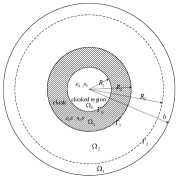
Figure 3.1: Sketch of the cross section.

3.2 Simulation of the spherical invisibility cloaks

In what follows, we focus on the simulation of the spherical cloaks. We first present the full model with reduction of the unbounded domain by using the NRBC in Section 2. As sketched in Figure 3.1, we denote

$$\begin{split}R_{0}=0;\;\;\Omega_{i}=\{R_{i}<r<R_{i+1}\},\;\;i=0,1;\\ \Omega_{2}=\Omega_{b_{0}}\setminus(\Omega_{0}\cup\Omega_{1}),\;\;\Omega_{3}=\Omega_{b}\setminus\Omega_{b_{0}}.\end{split}$$

Correspondingly, we further denote

$$\bm{F}(\bm{r},t)=\partial_{t}\bm{J}(\bm{r},t),$$

and

$$\begin{split}&\Gamma_{i}=\bar{\Omega}_{i}\cap\bar{\Omega}_{i+1},\quad\{\bm{E}^{i},\bm{H}^{i},\bm{D}^{i},\bm{B}^{i},\bm{F}^{i}\}=\{\bm{E},\bm{H},\bm{D},\bm{B},\bm{F}\}|_{\Omega_{i}},\;\;\;i=0,1,2;\\[2.0pt] &\{\bm{E}^{3},\bm{H}^{3},\bm{B}^{3},\bm{D}^{3},\bm{F}^{3}\}=\{\bm{E}^{\rm sc},\bm{H}^{\rm sc},\bm{B}^{\rm sc},\bm{D}^{\rm sc},\bm{F}\}|_{\Omega_{3}}.\end{split}$$ (3.27)

We summarise below the assumptions (for usual scattering problems):

• ${\bm{\varepsilon}}={\bm{\mu}}={\bm{I}}_{3}\;\;{\rm in}\;\;\Omega_{b}\setminus\Omega_{1}$;

• There is no wave in the truncated domain $\Omega_{b}$ at time $t=0$, that is, we shall have homogeneous initial condition;

• The source term $\bm{J}$ is compactly supported in $\Omega_{2}.$

Proposition 3.1.

The full model for 3D cloak takes the form

$$\partial_{t}^{2}{\bm{D}}^{i}+c^{2}\nabla\times\nabla\times\bm{D}^{i}=\bm{F}^{i}\quad{\rm in}\;\;\Omega_{i},\;\;i=0,2,3,$$ (3.28a)

$$\partial_{t}^{2}{\bm{D}}^{1}+c^{2}\nabla\times\big{(}\mathscr{D}_{2}[\nabla\times(\mathscr{D}_{1}[{\bm{D}}^{1}])]\big{)}=\bm{0}\quad{\rm in}\;\;\Omega_{1},$$ (3.28b)

$$({\bm{D}^{0}-\mathscr{D}_{1}[{\bm{D}}^{1}}])\times\hat{\bm{r}}=\bm{0},\;\;\big{(}\nabla\times\bm{D}^{0}-\mathscr{D}_{2}\big{[}\nabla\times\mathscr{D}_{1}[{\bm{D}}^{1}]\big{]}\big{)}\times\hat{\bm{r}}=\bm{0}\;\;{\rm on}\;\;\Gamma_{0},$$ (3.28c)

$$(\mathscr{D}_{1}[{\bm{D}}^{1}]-\bm{D}^{2})\times\hat{\bm{r}}=\bm{0},\;\;\big{(}\mathscr{D}_{2}\big{[}\nabla\times\mathscr{D}_{1}[{\bm{D}}^{1}]\big{]}-\nabla\times\bm{D}^{2}\big{)}\times\hat{\bm{r}}=\bm{0}\;\;{\rm on}\;\;\Gamma_{1},$$ (3.28d)

$$({\bm{D}}^{2}-\bm{D}^{3})\times\hat{\bm{r}}=\bm{D}^{\rm in}\times\hat{\bm{r}},\;\;\nabla\times({\bm{D}}^{2}-\bm{D}^{3})\times\hat{\bm{r}}=\nabla\times\bm{D}^{\rm in}\times\hat{\bm{r}}\;\;{\rm on}\;\;\Gamma_{2},$$ (3.28e)

$$\partial_{t}{\bm{D}}_{T}^{3}+c\big{(}\nabla\times{\bm{D}}^{3}\big{)}\times\hat{\bm{r}}-\mathscr{T}_{b}[{\bm{D}}^{3}]=\bm{0}\;\;\;{\rm at}\;\;r=b,$$ (3.28f)

$${\bm{D}}(\bm{r},0)=\bm{0},\quad\partial_{t}{\bm{D}}(\bm{r},0)=\bm{0}\;\;\;{\rm in}\;\;\Omega_{b},$$ (3.28g)

where $\bm{D}_{T}^{3}:=\hat{\bm{r}}\times\bm{D}^{3}\times\hat{\bm{r}}$ is the tangential component of $\bm{D}^{3}$ on the boundary $r=b$.

Proof.

Note that (3.28a) is a direct consequence of (1.6a), (3.28b) is proved in Theorem 3.1, and (3.28e)-(3.28g) are direct consequences of (1.6c)-(1.6e) and the above assumption (i). For the jump conditions (3.28c)-(3.28d), we recall the standard transmission conditions

$$\bm{E}^{i}\times\hat{\bm{r}}=\bm{E}^{i+1}\times\hat{\bm{r}},\quad\bm{H}^{i}\times\hat{\bm{r}}=\bm{H}^{i+1}\times\hat{\bm{r}}\quad{\rm at}\;\;\;\Gamma_{i},\quad i=0,1.$$ (3.29)

The first jump conditions in (3.28c)-(3.28d) can be obtained by directly applying the first constitutive relation between $\bm{E}$ and $\bm{D}$ to the above transmission condition on $\bm{E}$. Therefore, we focus on the first jump conditions in (3.28c)-(3.28d). Inserting the constitutive relations (3.8) into (3.29) directly leads to (3.28c) and

$$\bm{B}^{0}\times\hat{\bm{r}}=\mathscr{D}_{2}[\bm{B}^{1}]\times\hat{\bm{r}}\quad{\rm at}\;\;\;\Gamma_{1};\quad\bm{B}^{2}\times\hat{\bm{r}}=\mathscr{D}_{2}[\bm{B}^{1}]\times\hat{\bm{r}}\quad{\rm at}\;\;\;\Gamma_{2}.$$ (3.30)

From (3.23), we derive

$${\partial_{t}\bm{B}^{0}}\times\hat{\bm{r}}=\mathscr{D}_{2}\big{[}{\partial_{t}\bm{B}^{1}}\big{]}\times\hat{\bm{r}}\quad{\rm at}\;\;\;\Gamma_{1};\quad{\partial_{t}\bm{B}^{2}}\times\hat{\bm{r}}=\mathscr{D}_{2}\big{[}{\partial_{t}\bm{B}^{1}}\big{]}\times\hat{\bm{r}}\quad{\rm at}\;\;\;\Gamma_{2},$$ (3.31)

which, together with (1.6a) and (3.24), yields the second jump conditions in (3.28c)-(3.28d). This ends the derivation. ∎

3.2.1 VSH-spectral-element discretization

In view of the spherical geometry and radially stratified dispersive media, we can fully exploit these advantages to develop an efficient and accurate VSH-spectral-element solver for the Maxwell’s system (3.28). Needless to say, it is optimal compared with the FDTD simulation in [49, pp. 7307] for the time-domain Pendry’s spherical cloak.

The key is to employ the divergence-free VSH expansion of the fields and reduce the governing equations into two sequences of decoupled one-dimensional problems. By proposition 2.1, the solenoidal fields $\bm{D}^{i}$, $\bm{F}^{i}$ and $\bm{D}^{in}$ can have VSH expansions

$$\{\bm{D}^{i},\bm{F}^{i}\}=\{u_{00}^{i},f_{00}^{i}\}\,\bm{Y}_{0}^{0}+\sum_{l=1}^{\infty}\sum_{|m|=0}^{l}\Big{\{}\{u_{lm}^{i},f_{1,l}^{i,m}\}\,\bm{\Phi}_{l}^{m}+\nabla\times(\{v_{lm}^{i},f_{2,l}^{i,m}\}\,\bm{\Phi}_{l}^{m}\big{)}\Big{\}},$$ (3.32)

and

$$\bm{D}^{\rm in}=g_{00}\,\bm{Y}_{0}^{0}+\sum_{l=1}^{\infty}\sum_{|m|=0}^{l}\Big{\{}g_{lm}\,\bm{\Phi}_{l}^{m}+\nabla\times(h_{lm}\,\bm{\Phi}_{l}^{m}\big{)}\Big{\}}.$$ (3.33)

It is worthy of pointing out that the capacity operator in (3.28f) has two alternative expressions (2.7) and (2.35). Both use the usual VSH expansion coefficients. For example, we have

$$\mathscr{T}_{b}[\bm{D}^{3}]=\frac{c}{b}\sum_{l=1}^{\infty}\sum_{|m|=0}^{l}\bigg{\{}\frac{\omega_{l}\ast D_{lm}^{r}}{l(l+1)}\,{\bm{\Psi}}_{l}^{m}+\big{(}\sigma_{l}\ast D_{lm}^{(2)}\big{)}\,{\bm{\Phi}}_{l}^{m}\bigg{\}},$$ (3.34)

according to (2.35), where $\{D_{lm}^{r},D_{lm}^{(1)},D_{lm}^{(2)}\}$ are the coefficients in the VSH expansion

$$\bm{D}^{3}=D_{00}\bm{Y}_{0}^{0}+\sum_{l=1}^{\infty}\sum_{|m|=0}^{l}\bigg{\{}D_{lm}^{r}\,\bm{Y}_{lm}+D_{lm}^{(1)}\,{\bm{\Psi}}_{l}^{m}+D_{lm}^{(2)}\,{\bm{\Phi}}_{l}^{m}\bigg{\}}.$$ (3.35)

In order to do dimension reduction using expansion (3.32), we re-express the formulation (3.34) using coefficients $\{u_{lm}^{3},v_{lm}^{3}\}$. From the Proposition 2.1, we have relations

$$D_{lm}^{r}=\frac{l(l+1)}{r}v_{lm}^{3},\quad D_{lm}^{(1)}=\hat{\partial}_{r}v_{lm}^{3},\quad D_{lm}^{(2)}=u_{lm}^{3}.$$ (3.36)

A simple substitution in (3.34) gives

$${\mathscr{T}}_{b}[\bm{D}^{3}]=\frac{c}{b}\sum_{l=1}^{\infty}\sum_{m=-l}^{l}\bigg{\{}b^{-1}(\omega_{l}\ast v_{lm}^{3})\,{\bm{\Psi}}_{l}^{m}+\big{(}\sigma_{l}\ast u_{lm}^{3}\big{)}\,{\bm{\Phi}}_{l}^{m}\bigg{\}}.$$ (3.37)

Proposition 3.2.

For $l\geq 1$, $|m|\leq l$ and $i=0,1,2,3,$ denote

$$g=g_{lm},\;\;h=h_{lm},\;\;u^{i}=u_{lm}^{i},\;\;v^{i}=v_{lm}^{i},\;\;f_{1}^{i}=f_{1,l}^{i,m},\;\;f_{2}^{i}=f_{2,l}^{i,m},\;\;I_{i}:=(R_{i},R_{i+1}).$$ (3.38)

With the simple variable substitution

$$\tilde{u}^{0}=\epsilon u^{0},\quad\tilde{u}^{1}=u^{1},\quad\tilde{u}^{2}=\epsilon u^{2},\quad\tilde{u}^{3}=\epsilon u^{3},\quad\tilde{g}=\epsilon g,$$ (3.39)

the Maxwell system (3.28) reduced to the following two sequences of one-dimensional problem for $v$ and $\tilde{u}$, respectively, for $l\geq 1$, $|m|\leq l$:

$$\frac{\partial^{2}v^{i}}{\partial t^{2}}-\frac{c^{2}}{r^{2}}\frac{\partial}{\partial r}\Big{(}r^{2}\frac{\partial v^{i}}{\partial r}\Big{)}+\frac{c^{2}\beta_{l}}{r^{2}}v^{i}=f_{2}^{i},\quad r\in I_{i},\quad i=0,2,3,$$ (3.40a)

$$\frac{\partial^{2}v^{1}}{\partial t^{2}}-\frac{c^{2}}{\epsilon^{2}r^{2}}\frac{\partial}{\partial r}\Big{(}r^{2}\frac{\partial v^{1}}{\partial r}\Big{)}+\frac{c^{2}}{\epsilon}\frac{\beta_{l}}{r^{2}}v^{1}+\frac{c^{2}}{\epsilon}\frac{\beta_{l}}{r^{2}}\vartheta_{1}\ast v^{1}(r,t)=0,\quad r\in I_{1},$$ (3.40b)

$$v^{0}=v^{1},\quad\partial_{r}v_{1}=\epsilon\partial_{r}v^{0}+(\epsilon-1)r^{-1}v^{0}\quad{\rm at}\;\;\;r=R_{1},$$ (3.40c)

$$v^{2}=v^{1},\quad\partial_{r}v_{1}=\epsilon\partial_{r}v^{2}+(\epsilon-1)r^{-1}v^{2}\quad{\rm at}\;\;\;r=R_{2},$$ (3.40d)

$$v^{2}-v^{3}=h,\quad\partial_{r}v^{2}-\partial_{r}v^{3}=\partial_{r}h\quad{\rm at}\;\;\;r=R_{3},$$ (3.40e)

$$\frac{1}{c}\partial_{t}v^{3}+\frac{\partial v^{3}}{\partial r}+\frac{1}{b}v^{3}-\frac{1}{b}\sigma_{l}*v^{3}=0\quad{\rm at}\;\;\;r=b,$$ (3.40f)

$$v|_{t=0}=\partial_{t}v|_{t=0}=0.$$ (3.40g)

while $\tilde{u}$ satisfies the same equations in (3.40) with $\tilde{u},$ $f_{1},$ $\tilde{g}$ and $\vartheta_{2}$, in place of $v,$ $f_{2},$ $h$ and $\vartheta_{1}$, respectively, and for $l=m=0,$

$$\partial^{2}_{t}u_{00}^{i}=f_{00}^{i},\quad u^{i}_{00}|_{t=0}=\partial_{t}u^{i}_{00}|_{t=0}=0,\quad r\in I_{i}.$$ (3.41)

Proof.

We postpone the detailed derivation in B. ∎

The above proposition shows that $\tilde{u}$ and $v$ can be obtained by solving (3.40) with different input data. Therefore, we only need to focus on the one dimensional problems (3.40). Note that the solution of (3.40) has a jump at $r=R_{3}$. We introduce

$$\tilde{v}(r,t)=\begin{cases}\displaystyle v(r,t),\quad 0\leq r\leq R_{3},\quad t\geq 0,\\[4.0pt] \displaystyle v(r,t)+h(R_{3},t)\frac{b-r}{b-R_{3}},\quad R_{3}<r\leq b,\quad t\geq 0,\end{cases}$$ (3.42)

and

$$\tilde{f}_{2}(r,t)=\begin{cases}\displaystyle f_{2}(r,t),\quad 0<r<R_{3},\;\;t>0,\\[4.0pt] \displaystyle f_{2}(r,t)+\bigg{\{}\frac{\partial^{2}h(R_{3},t)}{\partial t}+\Big{(}\frac{2bc^{2}}{r(b-r)}+\frac{c^{2}\beta_{l}}{r^{2}}\bigg{)}h(R_{3},t)\bigg{\}}\frac{b-r}{b-R_{3}},\;\;R_{3}<r<b,\;\;t>0,\end{cases}$$

to rewrite (3.40) into

$$\frac{\partial^{2}\tilde{v}^{i}}{\partial t^{2}}-\frac{c^{2}}{r^{2}}\frac{\partial}{\partial r}\Big{(}r^{2}\frac{\partial\tilde{v}^{i}}{\partial r}\Big{)}+\frac{c^{2}\beta_{l}}{r^{2}}\tilde{v}^{i}=\tilde{f}_{2}^{i},\quad r\in I_{i},\;\;i=0,2,3,$$ (3.43a)

$$\frac{\partial^{2}\tilde{v}^{1}}{\partial t^{2}}-\frac{c^{2}}{\epsilon^{2}r^{2}}\frac{\partial}{\partial r}\Big{(}r^{2}\frac{\partial\tilde{v}^{1}}{\partial r}\Big{)}+\frac{c^{2}}{\epsilon}\frac{\beta_{l}}{r^{2}}\tilde{v}^{1}+\frac{c^{2}}{\epsilon}\frac{\beta_{l}}{r^{2}}\vartheta_{1}\ast\tilde{v}^{1}(r,t)=0,\quad r\in I_{1},$$ (3.43b)

$$\tilde{v}^{0}=\tilde{v}^{1},\quad\partial_{r}\tilde{v}_{1}=\epsilon\partial_{r}\tilde{v}^{0}+(\epsilon-1)r^{-1}\tilde{v}^{0}\quad{\rm at}\;\;\;r=R_{1},$$ (3.43c)

$$\tilde{v}^{2}=\tilde{v}^{1},\quad\partial_{r}\tilde{v}_{1}=\epsilon\partial_{r}\tilde{v}^{2}+(\epsilon-1)r^{-1}\tilde{v}^{2}\quad{\rm at}\;\;\;r=R_{2},$$ (3.43d)

$$\tilde{v}^{2}=\tilde{v}^{3},\quad\partial_{r}\tilde{v}^{2}-\partial_{r}\tilde{v}^{3}=\partial_{r}h+\frac{1}{b-R_{3}}h(R_{3},t)\quad{\rm at}\;\;\;r=R_{3},$$ (3.43e)

$$\frac{1}{c}\partial_{t}\tilde{v}^{3}+\frac{\partial\tilde{v}^{3}}{\partial r}+\frac{1}{b}\tilde{v}^{3}-\frac{1}{b}\sigma_{l}*\tilde{v}^{3}=-\frac{1}{b-R_{3}}h(R_{3},t)\quad{\rm at}\;\;\;r=b,$$ (3.43f)

$$\tilde{v}|_{t=0}=h(R_{3},0)\frac{b-r}{b-R_{3}}\chi_{[R_{3},b]},\quad\partial_{t}\tilde{v}|_{t=0}=\frac{\partial h(R_{3},0)}{\partial t}\frac{b-r}{b-R_{3}}\chi_{[R_{3},b]}.$$ (3.43g)

Here $\chi_{[R_{3},b]}$ is the indicator function which is equal to $1$ inside the interval $[R_{3},b]$ and vanish outside.

Obviously, $\tilde{v}(r,t)$ is continuous in $I$. Multiplying (3.43a) and (3.43b) by test function $r^{2}\phi$ and $\epsilon r^{2}\phi$ respectively for $\phi\in H^{1}(I)$, using integration by parts and summing up the resulted equations, then applying the interface conditions and boundary condition we obtain the variational problem: Find $\tilde{v}(\cdot,t)\in H^{1}(I)$, s.t.

$$\mathcal{B}(\tilde{v},\phi)=(\tilde{f}_{2},\phi)+\Big{(}\partial_{r}h(R_{3},t)+\frac{h(R_{3},t)}{b-R_{3}}\Big{)}c^{2}R_{3}^{2}\phi(R_{3})-\frac{h(R_{3},t)}{b-R_{3}}c^{2}b^{2}\phi(b),$$ (3.44)

for all $\phi\in H^{1}(I)$, where

$$\begin{split}\mathcal{B}(\tilde{v},\phi):=&\int_{I\backslash I_{1}}(r^{2}\partial_{tt}\tilde{v}\phi+c^{2}r^{2}\partial_{r}\tilde{v}\partial_{r}\phi)dr+\int_{I_{1}}\Big{(}\epsilon r^{2}\partial_{tt}\tilde{v}\phi+\frac{c^{2}r^{2}}{\epsilon}\partial_{r}\tilde{v}\partial_{r}\phi\Big{)}dr\\ +&\beta_{l}c^{2}\Big{(}\int_{I}\tilde{v}\phi dr+\int_{I_{1}}\vartheta_{1}\ast\tilde{v}(r,t)\phi(r)dr\Big{)}+c^{2}(\epsilon-1)R_{1}\tilde{v}(R_{1},t)\phi(R_{1})\\ -&c^{2}(\epsilon-1)R_{2}\tilde{v}(R_{2},t)\phi(R_{2})+\big{\{}cb^{2}\partial_{t}\tilde{v}(b,t)+c^{2}b(\tilde{v}(b,t)-\sigma\ast\tilde{v}(b,t))\big{\}}\phi(b).\end{split}$$ (3.45)

Based on the variational problem (3.44), we introduce the spectral-element discretization. Let $\mathcal{I}_{h}:0=r_{0}<r_{1}<\cdots<r_{E}=b$ be an interface conforming mesh of the interval $I$ and denote the element by $\{K_{e}=(r_{e-1},r_{e})\}_{e=1}^{E}$. Here, the interface conforming mesh means that the points $r=R_{1},R_{2},R_{3}$ are mesh points, see Figure 3.2. Let $\mathcal{P}_{N}(K_{e})$ be the set of all complex valued polynomials of degree at most $N$ in each interval $K_{e}$ and define the spectral element approximation space as

$$\mathscr{X}_{N}(\mathcal{I}_{h}):=\big{\{}u\in H^{1}(I):u|_{K_{e}}\in\mathcal{P}_{N}(K_{e})\big{\}}.$$ (3.46)

The spectral element discretization of (3.43) is to find $\tilde{v}_{N}(r,t)\in{\mathscr{X}}_{N}(\mathcal{I}_{h})$ for all $t>0$, such that

$$\mathcal{B}(\tilde{v}_{N},\phi)=(\tilde{f}_{2},\phi)+\Big{(}\partial_{r}h(R_{3},t)+\frac{h(R_{3},t)}{b-R_{3}}\Big{)}c^{2}R_{3}^{2}\phi(R_{3})-\frac{h(R_{3},t)}{b-R_{3}}c^{2}b^{2}\phi(b),$$ (3.47)

for all $\phi\in{\mathscr{X}}_{N}(\mathcal{I}_{h})$.

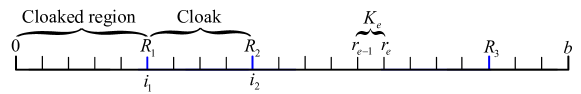
Figure 3.2: Interface conforming mesh used by the spectral element discretization.

This spectral element discretization for $\tilde{v}$ leads to the following integral differential system

$$\begin{split}&\mathbb{M}\ddot{\bm{V}}+\mathbb{B}\dot{\bm{V}}+{\mathbb{C}}{\bm{V}}+\bm{G}-\frac{c}{b}\mathbb{B}(\sigma\ast{\bm{V}})={\bm{F}},\quad\bm{V}(0)=\bm{V}_{0},\quad\dot{\bm{V}}(0)=\bm{V}_{1},\end{split}$$ (3.48)

where

$$\mathbb{M}=(m_{ij})_{\mathcal{N}\times\mathcal{N}},\quad\mathbb{A}=(a_{ij})_{\mathcal{N}\times\mathcal{N}},\quad\bm{G}=(G_{i})_{\mathcal{N}},$$

$$\mathbb{B}=cb^{2}\mathbb{E}_{\mathcal{N}\mathcal{N}},\quad\mathbb{C}=\mathbb{A}+c^{2}b\mathbb{E}_{\mathcal{N}\mathcal{N}}+c^{2}(\epsilon-1)(R_{1}\mathbb{E}_{i_{1}i_{1}}-R_{2}\mathbb{E}_{i_{2}i_{2}}),$$

are matrices with entries given by

$$\begin{split}&m_{ij}=\int_{I\backslash I_{1}}r^{2}\phi_{i}\phi_{j}dr+\epsilon\int_{I_{1}}r^{2}\phi_{i}\phi_{j}dr,\quad G_{i}=\beta_{l}c^{2}\int_{I_{1}}{\vartheta}_{1}\ast\tilde{v}_{N}(r,t)\phi_{i}(r)dr,\\ &a_{ij}=c^{2}\int_{I\backslash I_{1}}(r^{2}\partial_{r}\phi_{j}\partial_{r}\phi_{i}+\beta_{l}\phi_{j}\phi_{i})dr+c^{2}\int_{I_{1}}\Big{(}\frac{r^{2}}{\epsilon}\partial_{r}\phi_{j}\partial_{r}\phi_{i}+\beta_{l}\phi_{j}\phi_{i}\Big{)}dr,\\ &F_{i}=\int_{I}\tilde{f}_{2}\phi_{i}(r)dr+\Big{(}\partial_{r}h(R_{3},t)+\frac{h(R_{3},t)}{b-R_{3}}\Big{)}c^{2}R_{3}^{2}\phi_{i}(R_{3})-\frac{h(R_{3},t)}{b-R_{3}}c^{2}b^{2}\phi_{i}(b).\end{split}$$

Here, $i_{1}$, $i_{2}$ denote the global index of the freedom at $r=R_{1},R_{2}$ (see Figure 3.2 for illustration), respectively, $\mathcal{N}$ is the degree of freedom and also the global index of the freedom attached to mesh point $r=b$, and $\mathbb{E}_{mn}=(E_{ij})_{\mathcal{N}\times\mathcal{N}}$ is the matrix with only one non-zero entry $E_{mn}=1$.

3.2.2 Newmark’s scheme for time discretization

The spectral element discretization leads to the integral differential system (3.48) w.r.t $t$. Noting that all the involved time integrations are actually convolutions of exponential functions with the unknown functions, fast algorithm based on formula (2.29) can be used. Let us first discuss the discretization of the convolution ${\vartheta}_{1}\ast\tilde{v}_{N}(r,t)$. Define

$$\tilde{\vartheta}_{1}^{\alpha}(r,t)=e^{{\rm i}\zeta^{0}_{1}(r)t},\quad\tilde{\vartheta}_{1}^{\beta}(r,t)=e^{{\rm i}\zeta^{1}_{1}(r)t}.$$ (3.49)

Then

$${\vartheta}_{1}\ast\tilde{v}_{N}(r,t)=\frac{{\rm i}(\omega_{p,1}(r))^{2}}{\zeta^{0}_{1}(r)-\zeta^{1}_{1}(r)}\big{(}\tilde{\vartheta}_{1}^{\alpha}\ast\tilde{v}_{N}(r,t)-\tilde{\vartheta}_{1}^{\beta}\ast\tilde{v}_{N}(r,t)\big{)}.$$ (3.50)

By using the trapezoidal rule and (2.29), we have the second-order approximations

$$\begin{split}&\tilde{\vartheta}_{1}^{\alpha}\ast\tilde{v}_{N}(r,t_{n+1})\approx\lambda_{0}(r)\tilde{\vartheta}_{1}^{\alpha}\ast\tilde{v}_{N}(r,t_{n})+\frac{\Delta t}{2}(\tilde{v}_{N}(r,t_{n+1})+\lambda_{0}(r)\tilde{v}_{N}(r,t_{n})),\\ &\tilde{\vartheta}_{1}^{\beta}\ast\tilde{v}_{N}(r,t_{n+1})\approx\lambda_{1}(r)\tilde{\vartheta}_{1}^{\beta}\ast\tilde{v}_{N}(r,t_{n})+\frac{\Delta t}{2}(\tilde{v}_{N}(r,t_{n+1})+\lambda_{1}(r)\tilde{v}_{N}(r,t_{n})),\end{split}$$ (3.51)

where

$$\lambda_{0}(r)=e^{{\rm i}\zeta^{0}_{1}(r)\Delta t},\quad\lambda_{1}(r)=e^{{\rm i}\zeta^{1}_{1}(r)\Delta t}.$$ (3.52)

Substituting (3.51) into (3.50), we obtain

$${\vartheta}_{1}\ast\tilde{v}_{N}(r,t_{n+1})\approx\frac{{\rm i}(\omega_{p,1}(r))^{2}}{\zeta^{0}_{1}(r)-\zeta^{1}_{1}(r)}\big{(}\tilde{v}^{c}_{N}(r,t_{n})+\frac{\Delta t}{2}(\lambda_{0}(r)-\lambda_{1}(r))\tilde{v}_{N}(r,t_{n})\big{)},$$ (3.53)

where

$$\tilde{v}^{c}_{N}(r,t_{n}):=(\lambda_{0}(r)\tilde{\vartheta}_{1}^{\alpha}-\lambda_{1}(r)\tilde{\vartheta}_{1}^{\beta})\ast\tilde{v}_{N}(r,t_{n}).$$

Thus, we get the discretization for $\bm{G}(t_{n+1})$ given by $\bm{G}^{n+1}:=(G_{i}^{n+1})$ with

$$G_{i}^{n+1}:=\frac{{\rm i}\beta_{l}c^{2}(\omega_{p,1}(r))^{2}}{\zeta^{0}_{1}(r)-\zeta^{1}_{1}(r)}\int_{I_{1}}(v^{c}_{N}(r,t_{n})+\frac{\Delta t}{2}(\lambda_{0}(r)-\lambda_{1}(r))v_{N}(r,t_{n}))\phi_{i}(r)\,dr.$$ (3.54)

It is important to point out that $\bm{G}^{n+1}$ is a vector obtained by using the solution before the current time step thus can be moved to the right hand side in the fully discretization scheme. We denote the new right hand side vector by $\widetilde{\bm{F}}^{n}=\bm{F}^{n}-\bm{G}^{n}$.

Next, we consider the discretization of the convolution term $(\sigma_{l}\ast\bm{V})(t)$. For this purpose, we define

$${\bm{V}}_{j}(t):=\int_{0}^{t}e^{c(t-\tau)z_{j}^{l}/b}\bm{V}(\tau)\,d\tau.$$ (3.55)

By using the trapezoidal rule and (2.29) again, we obtain the second order approximations

$${\bm{V}}^{0}_{j}=\bm{0},\quad{\bm{V}}^{n+1}_{j}=e^{c\Delta tz_{j}^{l}/b}{\bm{V}}^{n}_{j}+\frac{\Delta t}{2}\bm{V}^{n+1}+\frac{\Delta t}{2}e^{c\Delta tz_{j}^{l}/b}\bm{V}^{n},\;\;$$ (3.56)

of ${\bm{V}}_{j}(t_{n+1})$ for $j=1,2,\cdots,l$. Accordingly, we have

$$(\sigma\ast{\bm{V}})^{0}=\bm{0},\quad(\sigma\ast{\bm{V}})^{n+1}=\frac{\Delta t}{2}\alpha_{1}\bm{V}^{n+1}+\frac{\Delta t}{2}\alpha_{2}\bm{V}^{n}+\sum_{j=1}^{l}\alpha_{2}^{j}{\bm{V}}^{n}_{j},$$ (3.57)

with

$$\alpha_{1}=\frac{c}{b}\sum_{j=1}^{l}z_{j}^{l},\quad\alpha_{2}^{j}=\frac{c}{b}z_{j}^{l}e^{c\Delta tz_{j}^{l}/b},\quad\alpha_{2}=\sum_{j=1}^{l}\alpha_{2}^{j},$$

is a second order discretization of the convolution term $(\sigma\ast{\bm{V}})(t_{n+1})$.

For the dicretization of time derivatives, we adopt the new marks scheme (cf. [40]). The key idea is to use the approximations:

$${\bm{V}}^{n+1} ={\bm{V}}^{n}+\Delta t\dot{\bm{V}}^{n}+\frac{\Delta t^{2}}{2}(1-2\beta)\ddot{\bm{V}}^{n}+\beta\Delta t^{2}\ddot{\bm{V}}^{n+1},$$ (3.58)

$$\dot{\bm{V}}^{n+1} =\dot{\bm{V}}^{n}+(1-\gamma)\Delta t\ddot{\bm{V}}^{n}+\gamma\Delta t\ddot{\bm{V}}^{n+1},$$ (3.59)

where $\beta$ and $\gamma$ are given parameters. Using the approximations (3.54) and (3.57), we can formulate the time discretization of the system (3.48) at $t_{n+1}$ as

$$\begin{split}\mathbb{M}\ddot{\bm{V}}^{n+1}+\mathbb{B}\dot{\bm{V}}^{n+1}+\mathbb{C}{\bm{V}}^{n+1}-\frac{c}{b}\mathbb{B}\bigg{\{}\frac{\alpha_{1}\Delta t}{2}\bm{V}^{n+1}+\frac{\alpha_{2}\Delta t}{2}\bm{V}^{n}+\sum\limits_{j=1}^{l}\alpha_{2}^{j}{\bm{V}}^{n}_{j}\bigg{\}}=\widetilde{\bm{F}}^{n+1}.\end{split}$$ (3.60)

Inserting (3.59) into (3.60) to eliminate $\dot{\bm{V}}^{n+1}$ leads to

$$\big{(}\mathbb{M}+\gamma\Delta t\mathbb{B}\big{)}\ddot{\bm{V}}^{n+1}+\Big{\{}\mathbb{C}-\frac{\alpha_{1}c\Delta t}{2b}\mathbb{B}\Big{\}}{\bm{V}}^{n+1}=\widetilde{\bm{F}}^{n+1}-\bm{W}^{n},$$ (3.61)

where

$$\bm{W}^{n}=(1-\gamma)\Delta t\mathbb{B}\ddot{\bm{V}}^{n}+\mathbb{B}\dot{\bm{V}}^{n}-\frac{\alpha_{2}c\Delta t}{2b}\mathbb{B}\bm{V}^{n}-\frac{c}{b}\mathbb{B}\sum\limits_{j=1}^{l}\alpha_{2}^{j}{\bm{V}}^{n}_{j}.$$

From (3.58), we have

$$\beta\Delta t^{2}\ddot{\bm{V}}^{n+1}=\bm{V}^{n+1}-\Big{\{}\bm{V}^{n}+\Delta t\dot{\bm{V}}^{n}+\Delta t^{2}\Big{(}\frac{1}{2}-\beta\Big{)}\ddot{\bm{V}}^{n}\Big{\}}:=\bm{V}^{n+1}-\widetilde{\bm{V}}^{n}.$$ (3.62)

Using (3.62) in (3.61) we arrive the fully discretization scheme

$$\bigg{\{}\mathbb{M}+\Big{(}\gamma\Delta t-\frac{\alpha_{1}c\beta\Delta t^{3}}{2b}\Big{)}\mathbb{B}+\beta\Delta t^{2}\mathbb{C}\bigg{\}}{\bm{V}}^{n+1}=\beta\Delta t^{2}\big{(}\widetilde{\bm{F}}^{n+1}-\bm{W}^{n}\big{)}+(\mathbb{M}+\gamma\Delta t\mathbb{B})\widetilde{\bm{V}}^{n}.$$ (3.63)

It is known that in general, the Newmark’s scheme is of second-order and unconditionally stable, if the parameter satisfy $\gamma\geq\frac{1}{2}$ and $\beta\geq\frac{1}{4}(\frac{1}{2}+\gamma)^{2}$.

4 Numerical experiments

In this section, we shall validate the feasibility and accuracy of the methodology for the simulation of 3D spherical cloaks via some numerical experiments. In all the experiments, we set $\varepsilon_{0}=\mu_{0}=1$, $c=1/\sqrt{\varepsilon_{0}\mu_{0}}=1$, $R_{3}=0.95$, $b=1$, $E=20$, $N=20$, $\triangle t=1.0e-3$. All VSH expansions are truncated at $L=40$ and the parameters in Newmark’s time discretization are set to $\gamma=0.5,\beta=0.25$.

4.1 Monochromatic incident wave

Set

$$\bm{D}^{\rm in}(\bm{r},t)=(1-e^{-10t})\cos(kx-\omega t)\bm{A},\quad\bm{A}:=\begin{bmatrix}0&0&A\end{bmatrix}^{\rm T},$$ (4.1)

where $k=\omega=40$ and $A=1$. Note that it gets close to a monochromatic wave very quickly as $t$ increases, e.g. $t>3,(1-e^{-10t})\geq 0.999999999999906$ due to the exponential term. The parameters of the cloaking device are set $\omega_{c}=40$, $\gamma_{1}=\gamma_{2}=0.001$, $R_{1}=0.15$, $R_{2}=0.35$. We plot the contours of $D_{z}$ at different time in Figure 4.1. It shows that the spherical domain $|\bm{r}|<R_{1}$ is perfectly cloaked from monochromatic wave with angular frequency $\omega=40$. No waves are propagating inside the cloaked region.

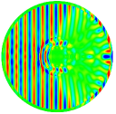
(a) t=1

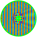
(b) t=3

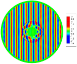
(c) t=5

(d) t=7

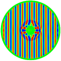
(e) t=9

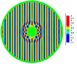
(f) t=11

Figure 4.1: Contours of the approximated $D_{z}$ in the $XY$ plane at different time steps with $R_{2}>2R_{1}$.

In the analysis of [23], a constraint $R_{2}\geq 2R_{1}$ is assumed. It was pointed out that it was unsure if this constraint is necessary and no numerical results regarding the case $R_{2}<2R_{1}$ were presented therein. Here, we shall do some numerical test for the case $R_{2}<2R_{1}$. For this purpose, we set $R_{1}=0.15$, $R_{2}=0.25<2R_{1}$ and plot the contours of $D_{z}$ at different time in Figure 4.2. It shows that the cloak works as well as in the case $R_{2}>2R_{1}$.

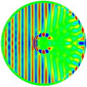
(a) t=1

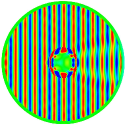
(b) t=3

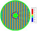
(c) t=5

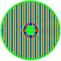
(d) t=7

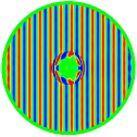
(e) t=9

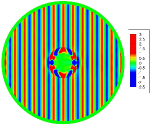
(f) t=11

Figure 4.2: Contours of the approximated $D_{z}$ in the $XY$ plane at different time steps with $R_{2}<2R_{1}$.

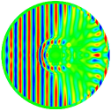
(a) t=1

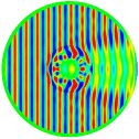
(b) t=3

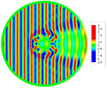
(c) t=5

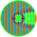
(d) t=7

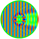
(e) t=9

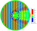
(f) t=11

Figure 4.3: Contours of the approximated $D_{z}$ in the $XY$ plane at different time steps with $k=38\neq\omega_{c}$.

As discussed in [49], the cloak is relatively sensitive to the frequency of the incident wave. Here we use the monochromatic incident wave (4.1) with $k=\omega=38$ to test the cloak device with parameters: $\omega_{c}=40$, $\gamma_{1}=\gamma_{2}=0.001$, $R_{1}=0.15$, $R_{2}=0.35$. The contours of the numerical $D_{z}$ at different time are plotted in Figure 4.3. The numerical results show that there are waves propagating inside the cloaking region.

4.2 Polychromatic incident wave

In this example, we use a pulse of plane wave given by

$$\bm{D}^{\rm in}=\mathfrak{Re}\{e^{{\rm i}k(x-t)}\}e^{-\frac{(x-t+t_{c})^{2}}{q}}\bm{A},\quad\bm{A}:=\begin{bmatrix}0&0&A\end{bmatrix}^{\rm T},$$

as the incident wave with $A=1$, $k=40$, $t_{c}=4$ and $q=0.5$. We first consider the cloaking device with parameters given by $\omega_{c}=40$, $\gamma_{1}=\gamma_{2}=0.001$, $R_{1}=0.15$, $R_{2}=0.35>2R_{1}$. The contours of $D_{z}$ at different time are plotted in Figure 4.4. Then, the outer radius of the cloak is set to $R_{2}=0.25<2R_{1}$ and other parameters remain unchanged. The contours of $D_{z}$ at different time are plotted in Figure 4.5. In these tests, there are polychromatic EM waves interacting with the cloaking devices. We can see from the numerical results that there are waves propagating inside the cloaked region.

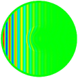
(a) t=3

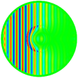
(b) t=3.5

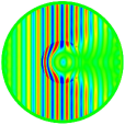
(c) t=4

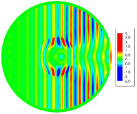
(d) t=4.5

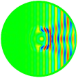
(e) t=5

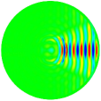
(f) t=5.5

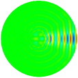
(g) t=6

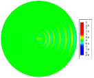
(h) t=6.5

Figure 4.4: Contours of the approximated $D_{z}$ in the $XY$ plane at different time steps with $R_{2}>2R_{1}$.

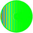
(a) t=3

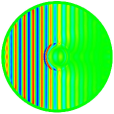
(b) t=3.5

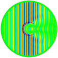
(c) t=4

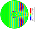
(d) t=4.5

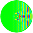
(e) t=5

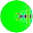
(f) t=5.5

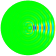
(g) t=6

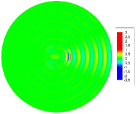
(h) t=6.5

Figure 4.5: Contours of the approximated $D_{z}$ in the $XY$ plane at different time steps with $R_{2}<2R_{1}$.

5 Conclusion

In this paper, we proposed accurate algorithms for computing the involved temporal convolutions of the NRBCs for the time-dependent Maxwell’s equations on a spherical artificial surface. More precisely, we provided the explicit formulas of the convolution kernel functions defined by inverse Laplace transforms of special modified Bessel functions, and also derived a new formulation of the NRBC capacity operator. With these at our proposal, the temporal convolutions in the NRBCs can be computed in a fast manner which therefore could offer an accurate way to reduce Maxwell’s system in $\mathbb{R}^{3}$ to a bounded domain. As a direct application of the truncated model, we considered the modelling and accurate simulation of the time-domain invisibility cloaks. We derived a new model valid for general cloaking geometry for the design of time-domain full wave invisibility cloaks involving just one unknown field $\bm{D}$ and seemingly complicated convolution operators that could be evaluated recursively in time again. In this work, we focused on the spherical invisibility cloaks designed in the first, original of Pendry et al (cf. [33]). We proposed an efficient VSH-spectral-element method for numerical simulation. The resulted algorithm could produce accurate numerical solution with far less computation cost compared with the simulations based on FDTD in literature.

Appendix A Vector spherical harmonics

We adopt the notation and setting as in Nédélec [28]. The spherical coordinates $(r,\theta,\varphi)$ are related to the Cartesian coordinates ${\bm{r}}=(x,y,z)$ via

$$x=r\sin\theta\cos\varphi,\quad y=r\sin\theta\sin\varphi,\quad z=r\cos\theta,$$ (A.1)

where $r\geq 0,\theta\in[0,\pi]$ and $\phi\in[0,2\pi).$ The corresponding moving (right-handed) orthonormal coordinate basis $\{{\bm{e}}_{r},{\bm{e}}_{\theta},{\bm{e}}_{\varphi}\}$ is given by

$$\begin{split}&{\bm{e}}_{r}=\hat{\bm{r}}={\bm{r}}/{r},\;\;{\bm{e}}_{\theta}=(\cos\theta\cos\varphi,\ \cos\theta\sin\varphi,\ -\sin\theta),\;\;{\bm{e}}_{\varphi}=(-\sin\varphi,\ \cos\varphi,\ 0).\end{split}$$ (A.2)

Let $\{Y_{l}^{m}\}$ be the spherical harmonics as normalized in [28], and let $S$ be the unit sphere. Recall that

$$\nabla_{S}Y_{l}^{m}=\frac{\partial Y_{l}^{m}}{\partial\theta}{\bm{e}}_{\theta}+\frac{1}{\sin\theta}\frac{\partial Y_{l}^{m}}{\partial\varphi}{\bm{e}}_{\varphi}.$$ (A.3)

The VSH family $\big{\{}\bm{Y}_{l}^{m},\bm{\Psi}_{l}^{m},\bm{\Phi}_{l}^{m}\big{\}}:=\big{\{}Y_{l}^{m}{\bm{e}}_{r},\nabla_{S}Y_{l}^{m},\nabla_{S}Y_{l}^{m}\times{\bm{e}}_{r}\big{\}},$ which has been used in the Spherepack [37] (also see [27]) forms a complete orthogonal basis of ${\bm{L}}^{2}(S):=(L^{2}(S))^{3}$ under the inner product:

$$\langle\bm{u},\bm{v}\rangle_{S}=\int_{S}\bm{u}\cdot\bar{\bm{v}}\,dS=\int_{0}^{2\pi}\int_{0}^{\pi}\bm{u}\cdot\bar{\bm{v}}\,\sin\theta\,d\theta d\varphi.$$ (A.4)

Define the subspace of ${\bm{L}}^{2}(S),$ consisting of the tangent components of the vector fields on $S$:

$${\bm{L}}_{T}^{2}(S)=\big{\{}\bm{u}\in{\bm{L}}^{2}(S):\bm{u}\cdot\hat{\bm{x}}=0\big{\}}.$$ (A.5)

The VSH $\{\bm{\Psi}_{l}^{m},{\bm{\Phi}}_{l}^{m}\}$ forms a complete orthogonal basis of ${\bm{L}}_{T}^{2}(S).$ Consequently, the vector field expanded in terms of VSH has a distinct separation of tangential and normal components. For any vector fields $\bm{u}\in{\bm{L}}^{2}(S)$, we write

$${\bm{u}}=u_{00}\bm{Y}_{0}^{0}+\sum_{l=1}^{\infty}\sum_{|m|=0}^{l}\big{\{}u_{lm}^{r}\,\bm{Y}_{l}^{m}\,+u_{lm}^{(1)}\bm{\Psi}_{l}^{m}+u_{lm}^{(2)}\,{\bm{\Phi}}_{l}^{m}\big{\}},$$ (A.6)

where we denote $\beta_{l}=l(l+1),$ and have

$$u_{00}=\langle\bm{u},\bm{Y}_{0}^{0}\rangle_{S},\;\;\;u_{lm}^{r}=\langle\bm{u},\bm{Y}_{l}^{m}\rangle_{S},\;\;\;u_{lm}^{(1)}={\beta_{l}^{-1}}\langle\bm{u},\bm{\Psi}_{l}^{m}\rangle_{S},\;\;\;u_{lm}^{(2)}={\beta_{l}^{-1}}\langle\bm{u},{\bm{\Phi}}_{l}^{m}\rangle_{S}.$$ (A.7)

It is noteworthy that given $\bm{u}$, we can be computed $\{u_{lm}^{r},u_{lm}^{(1)},u_{lm}^{(2)}\}$ via the discrete VSH-transform using the Spherepack [37], and vice versa by the inverse transform. Moreover, the normal component solely involves the first term while the tangential component $\bm{E}_{T}$ of $\bm{E}$ involves the last two terms in (A.6).

Now, we collect some frequently used vector calculus formulas. Define the differential operators:

$$d_{l}^{\pm}=\frac{d}{dr}\pm\frac{l}{r},\quad\hat{\partial}_{r}=\frac{d}{dr}+\frac{1}{r},\quad{\mathcal{L}}_{l}=\hat{\partial}_{r}^{2}-\frac{\beta_{l}}{r^{2}}=\frac{d^{2}}{dr^{2}}+\frac{2}{r}\frac{d}{dr}-\frac{\beta_{l}}{r^{2}},$$ (A.8)

where $\beta_{l}:=l(l+1)$. For any given $f(r)$, the following properties can be derived from [15]:

• For divergence operator

  $${\rm div}\big{(}f\bm{Y}_{l}^{m}\big{)}=\Big{(}\frac{d}{dr}+\frac{2}{r}\Big{)}f\,Y_{l}^{m},\quad{\rm div}\big{(}f\bm{\Psi}_{l}^{m}\big{)}=-\beta_{l}\frac{f}{r}\,\bm{Y}_{l}^{m},\quad{\rm div}\big{(}f\bm{\Phi}_{l}^{m}\big{)}=0;$$ (A.9)

• For curl operator

  $$\nabla\times\big{(}f\bm{Y}_{l}^{m}\big{)}=\frac{f}{r}\,\bm{\Phi}_{l}^{m},\quad\nabla\times\big{(}f\bm{\Psi}_{l}^{m}\big{)}=-\hat{\partial}_{r}f\,\bm{\Phi}_{l}^{m},\quad\nabla\times\big{(}f\bm{\Phi}_{l}^{m}\big{)}=\hat{\partial}_{r}f\,\bm{\Psi}_{l}^{m}+\beta_{l}\frac{f}{r}\bm{Y}_{l}^{m};$$ (A.10)

• For Laplace operator

  $$\Delta\big{(}f{\bm{\Phi}}_{l}^{m}\big{)}={\mathcal{L}}_{l}(f){\bm{\Phi}}_{l}^{m}.$$ (A.11)

Appendix B Proof of Proposition 3.2

Proof.

Recall that if ${\rm div}{\bm{u}}=0,$ then $\nabla\times\nabla\times{\bm{u}}=-\Delta{\bm{u}}.$ Thus, from (A.8)-(A.11), we derive

$$\nabla\times\nabla\times\big{(}u{\bm{\Phi}}_{l}^{m}\big{)}=-\Delta\big{(}u{\bm{\Phi}}_{l}^{m}\big{)}=-\mathcal{L}_{l}(u){\bm{\Phi}}_{l}^{m},$$

$$\nabla\times\nabla\times\nabla\times\big{(}v{\bm{\Phi}}_{l}^{m}\big{)}=-\nabla\times\big{(}\Delta\big{(}v{\bm{\Phi}}_{l}^{m}\big{)}\big{)}=-\nabla\times\big{(}\mathcal{L}_{l}\big{(}v\big{)}{\bm{\Phi}}_{l}^{m}\big{)}.$$

Therefore, (3.28a) can be reduced to:

$$\frac{\partial^{2}u^{i}_{lm}}{\partial t^{2}}-c^{2}\mathcal{L}_{l}(u^{i}_{lm})=f_{1,l}^{i,m}\quad\frac{\partial^{2}v^{i}_{lm}}{\partial t^{2}}-c^{2}\mathcal{L}_{l}(v^{i}_{lm})=f_{2,l}^{i,m},\quad r\in I_{i},\quad i=0,2,3,$$ (B.1)

for $|m|\leq l$, $l=1,2,\cdots$, by using the expansions (3.32). In spherical coordinates (cf. [1]):

$$\nabla\times{\bm{v}}=\frac{1}{r\sin\theta}\Big{(}\frac{\partial\big{(}\sin\theta v_{\varphi}\big{)}}{\partial\theta}-\frac{\partial v_{\theta}}{\partial\varphi}\Big{)}{\bm{e}}_{r}+\frac{1}{r}\Big{(}\frac{1}{\sin\theta}\frac{\partial v_{r}}{\partial\varphi}-\frac{\partial\big{(}rv_{\varphi}\big{)}}{\partial r}\Big{)}{\bm{e}}_{\theta}+\frac{1}{r}\Big{(}\frac{\partial\big{(}rv_{\theta}\big{)}}{\partial r}-\frac{\partial v_{r}}{\partial\theta}\Big{)}{\bm{e}}_{\varphi},$$ (B.2)

for any vector field $\bm{v}=v_{r}{\bm{e}}_{r}+v_{\theta}{\bm{e}}_{\theta}+v_{\varphi}{\bm{e}}_{\varphi}$. Apparently, we have $\nabla\times(u_{00}^{i}(r,t)\bm{Y}_{0}^{0})=\bm{0},$ as $\bm{Y}_{0}^{0}={\bm{e}}_{r}/\sqrt{4\pi}$. For the coefficient $u_{00}^{i}$, we then have

$$\frac{\partial^{2}u_{00}^{i}}{\partial t^{2}}=f_{00}^{i},\quad r\in I_{i},\quad i=0,2,3.$$ (B.3)

We now turn to the governing equation (3.28b) in the cloaking layer $I_{1}=(R_{1},R_{2})$. According to (A.10), the vector spherical harmonic expansion of $\bm{D}^{1}$ can be rewritten as

$${\bm{D}}^{1}=u_{00}^{1}\bm{Y}_{0}^{0}+\sum_{l=1}^{\infty}\sum_{|m|=0}^{l}\Big{\{}u_{lm}^{1}\bm{\Phi}_{l}^{m}+\hat{\partial}_{r}v_{lm}^{1}\bm{\Psi}_{l}^{m}+\frac{\beta_{l}}{r}v_{lm}^{1}\bm{Y}_{l}^{m}\Big{\}}.$$ (B.4)

Using (B.4) and the fact that $\mathscr{D}_{1}$ defined in (3.9) is uniaxial, we have

$$\mathscr{D}_{1}[{\bm{D}}^{1}]=\big{(}u_{00}^{1}+\theta_{1}\ast u_{00}^{1}\big{)}\bm{Y}_{0}^{0}+\sum_{l=1}^{\infty}\sum_{|m|=0}^{l}\Big{\{}\epsilon^{-1}u_{lm}^{1}\bm{\Phi}_{l}^{m}+\epsilon^{-1}\hat{\partial}_{r}v_{lm}^{1}\bm{\Psi}_{l}^{m}+\frac{\beta_{l}}{r}\big{(}v_{lm}^{1}+\theta_{1}\ast v_{lm}^{1}\big{)}\bm{Y}_{l}^{m}\Big{\}}.$$ (B.5)

Using formula (B.2), we have

$$\nabla\times\Big{(}\big{(}u_{00}^{1}+\theta_{1}\ast u_{00}^{1}\big{)}\bm{Y}_{0}^{0}\Big{)}=\bm{0}.$$ (B.6)

Then, we calculate from (B.5) that

$$\begin{split}\nabla\times\big{(}\mathscr{D}_{1}[{\bm{D}}^{1}]\big{)}=&\sum_{l=1}^{\infty}\sum_{|m|=0}^{l}\Big{(}\frac{\beta_{l}}{r^{2}}\big{(}v_{lm}^{1}+\theta_{1}\ast v_{lm}^{1}\big{)}-\epsilon^{-1}\hat{\partial}_{r}^{2}v_{lm}^{1}\Big{)}\bm{\Phi}_{l}^{m}\\ &+\sum_{l=1}^{\infty}\sum_{|m|=0}^{l}\Big{(}\epsilon^{-1}\hat{\partial}_{r}u_{lm}^{1}\bm{\Psi}_{l}^{m}+\epsilon^{-1}\frac{\beta_{l}}{r}u_{lm}^{1}\bm{Y}_{l}^{m}\Big{)}\end{split}$$ (B.7)

by using formulas (A.10). Repeating the above calculation and using the definition of $\mathscr{D}_{2}$ and (A.10), we obtain

$$\begin{split}\nabla\times\big{(}\mathscr{D}_{2}&\big{[}\nabla\times\big{(}\mathscr{D}_{1}[{\bm{D}}^{1}]\big{)}\big{]}\big{)}=\sum_{l=1}^{\infty}\sum_{|m|=0}^{l}\epsilon^{-1}\Big{(}\frac{\beta_{l}}{r^{2}}(u_{lm}^{1}+\theta_{2}\ast u_{lm}^{1})-\epsilon^{-1}\hat{\partial}_{r}^{2}u_{lm}^{1}\Big{)}\bm{\Phi}_{l}^{m}\\ &+\sum_{l=1}^{\infty}\sum_{|m|=0}^{l}\epsilon^{-1}\nabla\times\Big{(}\Big{(}\frac{\beta_{l}}{r^{2}}(v_{lm}^{1}+\theta_{1}\ast v_{lm}^{1})-\epsilon^{-1}\hat{\partial}_{r}^{2}v_{lm}^{1}\Big{)}\bm{\Phi}_{l}^{m}\Big{)},\end{split}$$ (B.8)

Inserting the above equation into (3.28b), one immediately shows that the expansion coefficients $\{u_{lm}^{1}$, $v_{lm}^{1}\},|m|\leq l,l=1,2,\cdots$ satisfy the same governing equation (3.40b) with different convolution kernels $\theta_{2}$ and $\theta_{1}$, respectively. As in (B.3), $u_{00}^{1}$ satisfies the same differential equation.

According to (B.4) and (B.5) and the facts

$$\bm{\Psi}_{l}^{m}\times\bm{e}_{r}=\bm{\Phi}_{l}^{m},\quad\bm{\Phi}_{l}^{m}\times\bm{e}_{r}=-\bm{\Psi}_{l}^{m},$$ (B.9)

we have

$$\begin{split}&{\bm{D}}^{i}\times\bm{e}_{r}=\sum_{l=1}^{\infty}\sum_{|m|=0}^{l}\big{(}-u_{lm}^{i}\bm{\Psi}_{l}^{m}+\hat{\partial}_{r}v_{lm}^{i}\bm{\Phi}_{l}^{m}\big{)},\quad i=0,2,3,\\ &(\nabla\times{\bm{D}}^{i})\times\bm{e}_{r}=\sum_{l=1}^{\infty}\sum_{|m|=0}^{l}\Big{\{}\Big{(}\hat{\partial}_{r}^{2}v_{lm}^{i}-\frac{\beta_{l}}{r^{2}}v_{lm}^{i}\Big{)}\bm{\Psi}_{l}^{m}+\hat{\partial}_{r}u_{lm}^{i}\bm{\Phi}_{l}^{m}\Big{\}},\quad i=0,2,3,\end{split}$$ (B.10)

and

$$\begin{split}&\mathscr{D}_{1}[{\bm{D}}^{1}]\times\bm{e}_{r}=\sum_{l=1}^{\infty}\sum_{|m|=0}^{l}\big{(}-\epsilon^{-1}u_{lm}^{1}\bm{\Psi}_{l}^{m}+\epsilon^{-1}\hat{\partial}_{r}v_{lm}^{1}\bm{\Phi}_{l}^{m}\big{)},\\ &\big{(}\nabla\times(\mathscr{D}_{1}[{\bm{D}}^{1}])\big{)}\times\bm{e}_{r}=\sum_{l=1}^{\infty}\sum_{|m|=0}^{l}\Big{\{}\Big{(}\epsilon^{-1}\hat{\partial}_{r}^{2}v_{lm}^{1}-\frac{\beta_{l}}{r^{2}}\big{(}v_{lm}^{1}+\theta_{1}\ast v_{lm}^{1}\big{)}\Big{)}\bm{\Psi}_{l}^{m}+\epsilon^{-1}\hat{\partial}_{r}u_{lm}^{1}\bm{\Phi}_{l}^{m}\Big{\}}.\end{split}$$

Substituting the above equations into jump condition (3.28c) and (3.28d), we obtain jump conditions

$$\begin{split}\epsilon u_{lm}^{0}=u_{lm}^{1},\quad\partial_{r}v_{lm}^{1}=\epsilon\partial_{r}v_{lm}^{0}+(\epsilon-1)r^{-1}v_{lm}^{0}\quad{\rm at}\;\;\;r=R_{1},\\ \epsilon u_{lm}^{2}=u_{lm}^{1},\quad\partial_{r}v_{lm}^{1}=\epsilon\partial_{r}v_{lm}^{2}+(\epsilon-1)r^{-1}v_{lm}^{2}\quad{\rm at}\;\;\;r=R_{2},\end{split}$$ (B.11)

and

$$\partial_{r}u_{lm}^{1}=\epsilon^{2}\partial_{r}u_{lm}^{0}+\epsilon(\epsilon-1)r^{-1}u_{lm}^{0}\quad{\rm at}\;\;\;r=R_{1},$$ (B.12)

$$\partial_{r}u_{lm}^{1}=\epsilon^{2}\partial_{r}u_{lm}^{2}+\epsilon(\epsilon-1)r^{-1}u_{lm}^{2}\quad{\rm at}\;\;\;r=R_{2},$$ (B.13)

$$\hat{\partial}_{r}^{2}v_{lm}^{0}-\frac{\beta_{l}}{r^{2}}v_{lm}^{0}=\epsilon^{-2}\hat{\partial}_{r}^{2}v_{lm}^{1}-\frac{\beta_{l}}{\epsilon r^{2}}\big{(}v_{lm}^{1}+\theta_{1}\ast v_{lm}^{1}\big{)}\quad{\rm at}\;\;\;r=R_{1},$$ (B.14)

$$\hat{\partial}_{r}^{2}v_{lm}^{2}-\frac{\beta_{l}}{r^{2}}v_{lm}^{2}=\epsilon^{-2}\hat{\partial}_{r}^{2}v_{lm}^{1}-\frac{\beta_{l}}{\epsilon r^{2}}\big{(}v_{lm}^{1}+\theta_{1}\ast v_{lm}^{1}\big{)}\quad{\rm at}\;\;\;r=R_{2}.$$ (B.15)

Noting that $\hat{\partial}_{r}^{2}u=\frac{1}{r^{2}}\frac{\partial}{\partial r}\big{(}r^{2}\frac{\partial u}{\partial r}\big{)}$, the governing equations (3.40a)-(3.40b) then gives

$$\begin{split}\epsilon^{-2}\hat{\partial}_{r}^{2}v_{lm}^{1}-\frac{\beta_{l}}{\epsilon r^{2}}\big{(}v_{lm}^{1}+\theta_{1}\ast v_{lm}^{1}\big{)}=\frac{1}{c^{2}}\frac{\partial^{2}v^{1}_{lm}}{\partial t^{2}},\quad\hat{\partial}_{r}^{2}v_{lm}^{i}-\frac{\beta_{l}}{r^{2}}v_{lm}^{i}=\frac{1}{c^{2}}\frac{\partial^{2}v^{i}_{lm}}{\partial t^{2}},\end{split}$$ (B.16)

for $i=0,2,3.$ Substituting (B.16) into the jump conditions (B.14)-(B.15) and integrate w.r.t. $t$ and using homogeneous initial conditions (3.40g), we derive

$$v^{0}_{lm}=v^{1}_{lm}\quad{\rm at}\;\;\;r=R_{1};\quad v^{2}_{lm}=v^{1}_{lm}\quad{\rm at}\;\;\;r=R_{2}.$$ (B.17)

Note that the jump conditions at artificial interface $r=R_{3}$ are trivial. Thus, we consider the boundary condition at $r=b$.

Applying expansion (3.32) in (3.28f) and using identities (B.9), (B.10) and formulation (3.37), we obtain

$$\begin{split}\sum_{l=1}^{\infty}\sum_{|m|=0}^{l}\!\Big{(}\partial_{t}\hat{\partial}_{r}v_{lm}^{3}+c\Big{(}\hat{\partial}_{r}^{2}v_{lm}^{3}-\frac{\beta_{l}}{b^{2}}v_{lm}^{3}\Big{)}-\frac{c}{b^{2}}\omega_{l}\ast v_{lm}^{3}\Big{)}\bm{\Psi}_{l}^{m}&\\ +\sum_{l=1}^{\infty}\sum_{|m|=0}^{l}\!\Big{(}\partial_{t}u_{lm}^{3}+c\hat{\partial}_{r}u_{lm}^{3}-\frac{c}{b}\sigma_{l}\ast u_{lm}^{3}\Big{)}\bm{\Phi}_{l}^{m}&=\bm{0},\end{split}$$ (B.18)

which implies two boundary conditions

$$\frac{1}{c}\partial_{t}u_{lm}^{3}+\frac{{\partial}u_{lm}^{3}}{\partial r}+\frac{1}{b}u_{lm}^{3}-\frac{1}{b}\sigma_{l}\ast u_{lm}^{3}=0\quad{\rm at}\;\;r=b,$$ (B.19)

$$\frac{\partial}{\partial r}\frac{\partial v_{lm}^{3}}{\partial t}+\frac{1}{b}\frac{\partial v_{lm}^{3}}{\partial t}+c\Big{(}\hat{\partial}_{r}^{2}v_{lm}^{3}-\frac{\beta_{l}}{b^{2}}v_{lm}^{3}\Big{)}-\frac{c}{b^{2}}\omega_{l}\ast v_{lm}^{3}=0\quad{\rm at}\;\;r=b.$$ (B.20)

Here, the definition of differential operator $\hat{\partial}$ in (A.8) is applied. Obviously, the boundary condition for $u_{lm}^{3}$ is exactly the one we adopted in the model problem (3.40). Next, we will show that the equation (B.20) can be reformulated to the same form as (B.19). Indeed, we can directly calculate

$$\frac{c}{b^{2}}\omega_{l}(t)\ast v_{lm}^{3}(b,t)=\frac{1}{b}\bigg{(}\int_{0}^{t}\sigma_{l}^{\prime}(t-\tau)v_{lm}^{3}(b,\tau)\,d\tau+\sigma_{l}(0)v_{lm}^{3}(b,t)\bigg{)}=\frac{1}{b}\partial_{t}(\sigma_{l}\ast v_{lm}^{3}(b,t)),$$ (B.21)

by using the expression of $\omega_{l}(t)$ (2.36). Using the above equation and (B.16) in (B.20) gives

$$\frac{\partial}{\partial t}\Big{\{}\frac{\partial v_{lm}^{3}}{\partial r}+\frac{1}{b}v_{lm}^{3}+\frac{1}{c}\frac{\partial v_{lm}^{3}}{\partial t}-\frac{1}{b}\sigma_{l}\ast v_{lm}^{3}\Big{\}}=0\quad{\rm at}\;\;r=b.$$ (B.22)

Consequently, we obtain boundary condition (3.40f) by the zero initial data assumption.

Note that the initial boundary value problems for coefficients $u_{lm}^{i}$ and $v_{lm}^{i}$ have almost the same form except the interface conditions (B.11)-(B.13) and (B.17). Apparently, by introducing the variable substitution (3.39), $\{\widetilde{u}_{lm}^{i}\}$ satisfy the same governing equation as $\{u_{lm}^{i}$ and the same interface and boundary conditions as $v_{lm}^{i}$. ∎

References

- [1] M. Abramowitz and I. Stegun. Handbook of Mathematical Functions. Dover, New York, 1964.
- [2] B. Alpert, L. Greengard, and T. Hagstrom. Rapid evaluation of nonreflecting boundary kernels for time-domain wave propagation. SIAM J. Numer. Anal., 37(4):1138–1164, 2000.
- [3] B. Alpert, L. Greengard, and T. Hagstrom. Nonreflecting boundary conditions for the time-dependent wave equation. J. Comput. Phys., 180(1):270–296, 2002.
- [4] G.B. Arfken and H.J. Weber. Mathematical Methods for Physicists. Academic Press, 1999.
- [5] J.P. Berenger. A perfectly matched layer for the absorption of electromagnetic waves. J. Comput. Phys., 114(2):185–200, 1994.
- [6] D. Colton and R. Kress. Inverse Acoustic and Electromagnetic Scattering Theory, volume 93 of Applied Mathematical Sciences. Springer-Verlag, Berlin, second edition, 1998.
- [7] S.A. Cummer, B.I. Popa, D. Schurig, D.R. Smith, and J.B. Pendry. Full-wave simulations of electromagnetic cloaking structures. Phys. Rev. E, 74(3):036621, 2006.
- [8] B. Engquist and A. Majda. Absorbing boundary conditions for the numerical simulation of waves. Math. Comp., 31(139):629–651, 1977.
- [9] A. Greenleaf, Y. Kurylev, M. Lassas, and G. Uhlmann. Cloaking devices, electromagnetic wormholes, and transformation optics. SIAM Rev., 51(1):3–33, 2009.
- [10] A. Greenleaf, M. Lassas, and G. Uhlmann. Anisotropic conductivities that cannot be detected by eit. Physiol. Meas., 24(2):413, 2003.
- [11] M.J. Grote and J.B. Keller. On non-reflecting boundary conditions. J. Comput. Phys., 122:231–243, 1995.
- [12] T. Hagstrom. Radiation boundary conditions for the numerical simulation of waves. Acta Numer., 8:47–106, 1999.
- [13] T. Hagstrom and S. Lau. Radiation boundary conditions for Maxwell’s equations: a review of accurate time-domain formulations. J. Comput. Math., 25(3):305–336, 2007.
- [14] Y. Hao and R. Mittra. FDTD Modeling of Metamaterials: Theory and Applications. Artech House, 2008.
- [15] E.L. Hill. The theory of vector spherical harmonics. Amer. J. Phys., 22:211–214, 1954.
- [16] S.D. Jiang and L. Greengard. Efficient representation of nonreflecting boundary conditions for the time-dependent Schrödinger equation in two dimensions. Commun. Pure Appl. Math., 61(2):261–288, 2008.
- [17] R.V. Kohn, D. Onofrei, M.S. Vogelius, and M.I. Weinstein. Cloaking via change of variables for the helmholtz equation. Commun. Pure and Appl. Math., 63(8):973–1016, 2010.
- [18] U. Leonhardt. Optical conformal mapping. Science, 312(5781):1777–1780, 2006.
- [19] J.C. Li and Y.Q. Huang. Time-domain Finite Element Methods for Maxwell’s Equations in Metamaterials, volume 43. Springer Science & Business Media, 2012.
- [20] J.C. Li. Error analysis of fully discrete mixed finite element schemes for 3D Maxwell’s equations in dispersive media. Comput. Methods Appl. Mech. Engrg., 196(33):3081–3094, 2007.
- [21] J.C. Li, Y.Q. Huang, and W. Yang. Developing a time-domain finite-element method for modeling of electromagnetic cylindrical cloaks. J. Comput. Phys., 231(7):2880–2891, 2012.
- [22] J.C. Li, Y.Q. Huang, and W. Yang. An adaptive edge finite element method for electromagnetic cloaking simulation. J. Comp. Phys., 249:216–232, 2013.
- [23] J.C. Li, Y.Q. Huang, and W. Yang. Well-posedness study and finite element simulation of time-domain cylindrical and elliptical cloaks. Math. Comp., 84(292):543–562, 2015.
- [24] J.C. Li, C. Meng, and Y.Q. Huang. Improved analysis and simulation of a time-domain carpet cloak model. Comput. Methods Appl. Math., 19(2):359–378, 2019.
- [25] H.Y. Liu and T. Zhou. On approximate electromagnetic cloaking by transformation media. SIAM J. Appl. Math., 71(1):218–241, 2011.
- [26] P. Monk. Finite Element Methods for Maxwell’s Equations. Numerical Mathematics and Scientific Computation. Oxford University Press, New York, 2003.
- [27] P.M. Morse and H. Feshbach. Methods of Theoretical Physics. 2 volumes. McGraw-Hill Book Co., Inc., New York, 1953.
- [28] J.C. Nédélec. Acoustic and Electromagnetic Equations, volume 144 of Applied Mathematical Sciences. Springer-Verlag, New York, 2001. Integral representations for harmonic problems.
- [29] N. Okada and J.B. Cole. FDTD modeling of a cloak with a nondiagonal permittivity tensor. ISRN. Opt., 2012:063903, 2012.
- [30] F.W.J. Olver, D.W. Lozier, R.F. Boisvert, and C.W. Clark. NIST Handbook of Mathematical Functions. Cambridge University Press, 2010.
- [31] S.J. Orfanidis. Electromagnetic Waves and Antennas. Rutgers University, 2002.
- [32] J.B. Pendry, A.J. Holden, W.J. Stewart, and I. Youngs. Extremely low frequency plasmons in metallic mesostructures. Phys. Rev. Lett., 76(25):4773, 1996.
- [33] J.B. Pendry, D. Schurig, and D.R. Smith. Controlling electromagnetic fields. Science, 312(5781):1780–1782, 2006.
- [34] M. Rahm, S.A. Cummer, D. Schurig, J.B. Pendry, and D.R. Smith. Optical design of reflectionless complex media by finite embedded coordinate transformations. Phys. Rev. Lett., 100(6):063903, 2008.
- [35] Z.C. Ruan, M. Yan, C.W. Neff, and M. Qiu. Ideal cylindrical cloak: perfect but sensitive to tiny perturbations. Phys. Rev. Lett., 99(11):113903, 2007.
- [36] I.L. Sofronov. Artificial boundary conditions of absolute transparency for two- and three-dimensional external time-dependent scattering problems. European J. Appl. Math., 9(6):561–588, 1998.
- [37] P.N. Swarztrauber and W.F. Spotz. Generalized discrete spherical harmonic transforms. J. Comput. Phys., 159(2):213–230, 2000.
- [38] T. Tokita. Exponential decay of solutions for the wave equation in the exterior domain with spherical boundary. J. Math. Kyoto Univ., 12(2):413–430, 1972.
- [39] M. Tsang and D. Psaltis. Magnifying perfect lens and superlens design by coordinate transformation. Phys. Rev. B., 77(3):035122, 2008.
- [40] L.L. Wang, B. Wang, and X.D. Zhao. Fast and accurate computation of time-domain acoustic scattering problems with exact nonreflecting boundary conditions. SIAM J. Appl. Math., 72(6):1869–1898, 2012.
- [41] G.N. Watson. A Treatise of the Theory of Bessel Functions (second edition). Cambridge University Press, Cambridge, UK, 1966.
- [42] M. Yan, W. Yan, and M. Qiu. Cylindrical superlens by a coordinate transformation. Phys. Rev. B., 78(12):125113, 2008.
- [43] W. Yang, J.C. Li, and Y.Q. Huang. Mathematical analysis and finite element time domain simulation of arbitrary star-shaped electromagnetic cloaks. SIAM J. Numer. Anal., 56(1):136–159, 2018.
- [44] Z.G. Yang and L.L. Wang. Accurate simulation of circular and elliptic cylindrical invisibility cloaks. Comm.Comp. Phys., 17(3):822?49, 2015.
- [45] Z.G. Yang, L.L. Wang, Z.J. Rong, B. Wang, and B.L. Zhang. Seamless integration of global Dirichlet-to-Neumann boundary condition and spectral elements for transformation electromagnetics. Comput. Methods Appl. Mech. Engrg., 301:137–163, 2016.
- [46] Y.B. Zhai, X.W. Ping, W.X. Jiang, and T.J. Cui. Finite-element analysis of three-dimensional axisymmetrical invisibility cloaks and other metamaterial devices. Commun. Comput. Phys., 8(4):823–834, 2010.
- [47] B.L. Zhang, B.I. Wu, H.S. Chen, and J.A. Kong. Rainbow and blueshift effect of a dispersive spherical invisibility cloak impinged on by a nonmonochromatic plane wave. Phys. Rev. Lett., 101(6):063902, 2008.
- [48] Y. Zhao, C. Argyropoulos, and Y. Hao. Full-wave finite-difference time-domain simulation of electromagnetic cloaking structures. Opt. Express, 16(9):6717–6730, 2008.
- [49] Y. Zhao and Y. Hao. Full-wave parallel dispersive finite-difference time-domain modeling of three-dimensional electromagnetic cloaking structures. J. Comp. Phys., 228(19):7300–7312, 2009.