General Probabilistic Theories with a Gleason-type Theorem
Abstract
Gleason-type theorems for quantum theory allow one to recover the quantum state space by assuming that (i) states consistently assign probabilities to measurement outcomes and that (ii) there is a unique state for every such assignment. We identify the class of general probabilistic theories which also admit Gleason-type theorems. It contains theories satisfying the no-restriction hypothesis as well as others which can simulate such an unrestricted theory arbitrarily well when allowing for post-selection on measurement outcomes. Our result also implies that the standard no-restriction hypothesis applied to effects is not equivalent to the dual no-restriction hypothesis applied to states which is found to be less restrictive.
1 Introduction
More than sixty years ago, Mackey [1] asked whether the density operator represents the most general notion of a quantum state that is consistent with the standard description of observables as self-adjoint operators. Gleason [2] responded with a proof that—in separable Hilbert spaces of dimension greater than two—every state must admit an expression in terms of a density operator if it is to consistently assign probabilities to the measurement outcomes of such observables. In 2003, Busch [3] (and then Caves et al. [4]) generalized the idea of Gleason’s theorem to observables represented by positive-operator measures (POMs). The resulting Gleason-type theorem (GTT) not only is much simpler to prove but it also applies to two-dimensional Hilbert spaces, since the assumptions being made are stronger than in Gleason’s case.
In this paper, we investigate whether the Gleason-type theorem is special to quantum theory. Imagine that a theory different from quantum theory were to successfully describe Nature. Would a GTT still exist?
Our question is made explicit by posing it within the family of general probabilistic theories (GPTs) which have emerged as natural generalizations of quantum theory [5, 6, 7, 8, 9]. The framework of GPTs derives from operational principles and it encompasses both quantum and classical models. One of the motivations to explore these alternative theories has been to identify features which single out quantum theory among others of comparable structure. Our study contributes to that fundamental quest.
Effectively, Gleason and Busch establish a bijection between frame functions and density operators in quantum theory. Frame functions associate probabilities to the mathematical objects representing the possible outcomes of measurements in such a way that the probabilities assigned to all disjoint outcomes of a given measurement sum to unity. The rationale behind a frame function is that the probabilities of all measurement outcomes for all observables should define a unique state. If this were not the case, then two “different” states would be indistinguishable, both practically and theoretically.
Our strategy will be to generalise the concept of frame functions to GPTs in order to investigate whether they are in exact correspondence with the objects that represent states in these theories. We are able to identify all general probabilistic theories in which this correspondence continues to hold. We find that GTTs exist for GPTs satisfying the no-restriction hypothesis [10, 11], as anyone familiar with the proof of Busch’s result or the work of Gudder et al. [12] might expect. However, we also find other GPTs which admit a Gleason-type theorem, namely those that satisfy a “noisy version” of the no-restriction hypothesis (or come arbitrarily close to satisfying it). An alternative way to characterise this class of GPTs is to use the idea of simultation of measurements via classical processes and postselection [13]. Any GPT in this class can simulate an arbitrarily good approximation to any observable in a related unrestricted GPT (i.e. the GPT satisfying the no-restriction hypothesis).
The existence of a GTT for GPTs such as quantum theory or real-vector-space quantum theory [14, 15, 16, 17] has a number of consequences. It becomes possible, for example, to modify the axiomatic structure of the theories as it is no longer necessary to—separately and independently—stipulate both the state space and the observables of the theory. Our result can also be used to derive the standard GPT framework from operational assumptions different to those found in the literature. More specifically, the standard GPT framework is recovered if—after motivating the standard description of observables in GPTs—states are assumed to correspond to frame functions of these observables.
Additionally, our result also uncovers a new property of the no-restriction hypothesis in GPTs. The standard no-restriction hypothesis applied to effects turns out to be inequivalent to the dual assumption—the no-state-restriction hypothesis—applied to states. Consequently, deriving the GPT framework in two equivalent ways, starting from the structure of state spaces in one case or effect spaces in the other, leads to inequivalent frameworks if the respective no-restriction hypotheses are assumed.
To make the paper self-contained and to introduce the notation, we will first review concepts of the GPT framework relevant here. In Section 4, we define frame functions for GPTs and prove our main theorem. In Section 5, we provide three examples to demonstrate the simplification of the postulates required to specify an individual GPT. Section 6 strengthens our main theorem by defining frame functions only on a proper subset of all observables, the analog of projective-simulable observables. The stronger result leads to an alternative operational motivation for deriving part of the GPT framework. In Section 7 we summarize and discuss our results.
2 General probabilistic theories
The GPT framework allows one to define a broad family of theories of which quantum theory (in finite dimensional Hilbert spaces) is a member. Any (real or fictitious) system described by a GPT has the following fundamental property: there exists a finite set of fiducial measurement outcomes, the probabilities of which uniquely determine its state.111To encompass quantum theory in toto, the restriction to a finite set of fiducial measurement outcomes would need to be relaxed; see Nuida et al. [18] and Lami et al. [19], for example. For example, the state of a spin- particle is determined by the probabilities of the outcome of measuring spin observables in three orthogonal directions, as demonstrated by the Bloch vector description.
There are many different yet equivalent ways to formulate the GPT framework. To make this paper self-contained, let us briefly outline an intuitive approach to GPTs which is based on an operational derivation [7].
2.1 States
If a system has a minimal fiducial set consisting of outcomes222A fiducial set is minimal if there is no such set with fewer than outcomes., its state space is given by a convex, compact set of vectors of the form
| (1) |
where , are the probabilities of the fiducial outcomes. The extra dimension of the “ambient” vector space simplifies the description of measurement outcomes, as explained below. The convexity of the state space follows from the assumption that if one were to prepare the system in the states and with probabilities and , respectively, then the probability of observing the -th fiducial measurement outcome should equal
| (2) |
therefore, this mixed state should be represented by the vector
| (3) |
A state is extremal if it cannot be written as a (non-trivial) convex combination of other states. The state space is assumed to be compact since, firstly, it must be bounded if the entries of the vector are to be between zero and one. Secondly, as an arbitrarily good approximation of a state would be operationally indistinguishable from the state itself, we also assume the state space is closed in the Euclidean topology. Throughout the manuscript we will use the Euclidean topology and Euclidean norm .
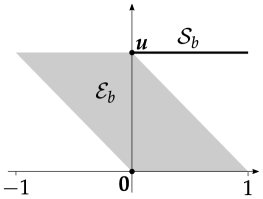
As an example, consider a classical bit which may reside in one of two states called “0” and “1”, or in a mixture of the two. If we know that the bit is in state 0 with probability then it is in state 1 with probability ; in other words, the number determines the state of the system. When performing the measurement which asks “Is the bit in state 0 or 1?”, the outcome “The bit is in state 0.” forms a complete set of fiducial measurement outcomes. Thus, the state space of the bit can be represented by the line segment between and , as displayed in Fig. 1a (see Section. 2.2). The end points of the segment correspond to the states 0 and 1, respectively, and their convex hull defines the state space .
2.2 Effects and observables
The possible outcomes of measuring an observable in a GPT system with state space correspond to effects which are linear maps such that for all states ; here denotes the probability of observing the outcome when a measurement (with as a possible outcome) is performed on a system in state . Due to the linearity of the map , any effect can be uniquely expressed in the form
| (4) |
for some vector . We will also use the term “effect” to refer to the vector representing a map .
The linearity of effects is motivated by the assumption that they should respect the mixing of states with some parameter . More specifically, the following two events should occur with the same probability:
-
(i)
observing the outcome of a measurement performed on a system in a mixed state ;
-
(ii)
observing the outcome when the measurement is performed with probability on a system in state and with probability on a system prepared in state .
This assumption implies that the map should satisfy
| (5) |
Thus, the map is an affine function on the state space which can be extended to a linear function on the vector space containing .
The set of all effects associated with measurement outcomes in a specific GPT system is known as its effect space, . The space corresponds to a convex subset of , as does the state space . It necessarily contains the zero and unit vectors,
| (6) |
as well as the vector for every [11], which arises automatically as a valid effect. We also assume that the effect space spans the full dimensions of the vector space; otherwise the model would contain states which result in identical probabilities for all effects in the effect space, making them indistinguishable and hence operationally equivalent. Note that a -dimensional state space comes with a -dimensional effect space. Extremal effects are defined by the property that they cannot be written as a (non-trivial) convex combination of other effects.
Observables are given by tuples of elements of the effect space that sum to the unit effect , with each effect in the tuple corresponding to a different possible outcome when measuring the observable. The position of an effect in the tuple encodes the label of the corresponding outcome. Given the observable , for example, we will say effect represents the first possible outcome of measuring since occupies the first position in the tuple. A GPT should also specify which tuples of effects correspond to observables (or, in the language of [20], the GPT should specify the set of meters). We will assume throughout (except in Section. 6) that any finite tuple of effects satisfying
| (7) |
and
| (8) |
for any subset , corresponds to an observable of the GPT system333This assumption is equivalent to considering GPTs with a restriction of type (R1) in [20], whereas the GPTs considered in Section. 6 can be of type (R2) or (R3).. Eq. (8) ensures that the set of observables is closed under coarse-graining of outcomes.
The effect space of the classical bit with state space is given by the parallelogram depicted in Fig. 1a. The two-outcome measurement answering “Is the bit in state 0 or 1?” is represented by
| (9) |
2.3 Equivalent GPTs
When considering a specific GPT it is sometimes useful to linearly transform its state and effect spaces. The Bloch vector describing a qubit state is a case in point since its components do not necessarily take values in the range . The Bloch vector representation of a qubit density operator
| (10) |
is given by the vector , with the fourth component being the coefficient of the identity matrix. The linear relation between each of the coefficients and the probability of finding the outcome “” when measuring reads explicitly .
Any linear transformation which preserves the inner product between states and effects of a given GPT system gives rise to an alternative representation. Suppose that we transform the state space by an invertible matrix to the space . Then we must apply the inverse transpose transformation to the effect space, , in order that the probabilities remain invariant,
| (11) |
The transformed state and effect spaces continue to be convex subsets of , and they can even be thought of as a convex subset of a vector space isomorphic to . GPTs are often presented in this way (cf. [21, 11] and references therein).
The standard formulation of quantum theory in finite dimensions is an example of representing the state and effect spaces of a theory as subsets of a vector space isomorphic to . Quantum states are represented by density operators on which form a convex subset of the real vector space of Hermitian operators on , which is isomorphic to . Quantum effects, or elements of a positive-operator measure (POM), can also be embedded in this space with for an operator satisfying for all rays . Using this representation of the state and effect spaces is convenient for since it is cumbersome to explicitly describe the set of density operators by some set of constraints on vectors of the form given in Eq. (1) (see e.g. [22, 23, 24]).
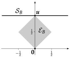
As an explicit example, let us transform the GPT description of a classical bit with state space by the matrix
| (12) |
The new state space, , is now the convex hull of the images of the extremal states and (previously located at and , respectively), i.e.
| (13) |
Similarly, the effect space, , is given by the convex hull of the zero effect , the unit effect and two other extremal effects,
| (14) |
as pictured in Figure 1b.
2.4 Cones in GPTs
The notion of a positive cone is useful when studying the properties of state and effect spaces of a GPT. A positive cone is a subset of that contains all non-negative linear combinations of its elements (see [25], in which our positive cone corresponds to a cone containing the origin). Positive cones may, for example, be generated from convex subsets of real vector spaces.
Definition 1.
The positive cone of a convex subset of a real vector space is the set of vectors
| (15) |
Positive cones also arise from considering the space dual to a subset of vectors in an inner product space.
Definition 2.
The dual cone of a subset of a real inner product space is the positive cone
| (16) |
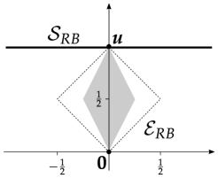
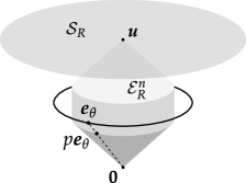
Figure (2a) illustrates, for a classical bit, the dual cone of the state space . It is easy to see that, in general, the effect space of a GPT system must be contained within the dual cone of the state space in order that the effects assign non-negative probabilities to every state in the state space.
The following lemma describes a simple but important property of effect spaces related to the fact that the elements of its dual cone effectively span the ambient space.
Lemma 1.
For any effect space and any vector , we have for some vectors .
Proof.
Firstly, the interior of is non-empty since is convex and spans . Let be an interior point of . As is an interior point of , we have that for some and we may take and . ∎

Two further lemmata (proven in Appendix A), which we will need later on, establish relations between positive cones and their dual cones. We will denote the closure of a set by .
Lemma 2.
Let be a compact, convex subset of , then .
Lemma 3.
For a compact and convex subset , we have .
Finally, it will also be important that the positive cone of a GPT state space is always a closed set (also proven in Appendix A).
Lemma 4.
Given a GPT state space , the positive cone is closed.
3 Unrestricted GPTs
The main result of this paper is to establish a Gleason-type theorem for a class of GPTs which we will introduce in this section, namely almost noisy unrestricted GPTs. First, we describe the no-restriction hypothesis and the unrestricted GPTs it defines. Next, we define noisy unrestricted (NU) GPTs and, building on this concept, we define almost NU GPTs.
3.1 The no-restriction hypothesis
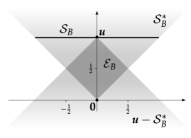
A particularly close relationship between state and effect spaces exists in GPTs that satisfy the no-restriction hypothesis [11], i.e. GPTs with effect spaces consisting of all linear maps such that for all . In such an unrestricted theory the state space defines a unique effect space, and vice versa. The effect space of a system with state space in an unrestricted GPT is given by
| (17) |
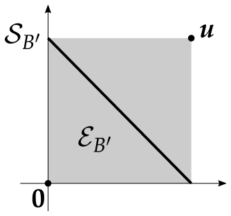
where . The classical bit is an example of an unrestricted GPT system. The cones and as well as their intersection are illustrated in Figure 2b.
Conversely, if an unrestricted GPT system has an effect space then a unique state space is associated with it, namely:
| (18) |
where ; we will omit the subscript whenever the dimension is clear from the context. We have introduced the maps and in the context of unrestricted GPTs but they are well-defined for the state and effect spaces of any GPT. The maps will play an important role in the derivation of our main result (see Section 4).
3.2 Noisy unrestricted GPTs
The class of NU GPTs consists of all unrestricted GPTs along with a special subset of restricted GPTs. The included restricted GPTs are those that can be thought of as unrestricted GPTs in which some (or all) of the observables can only be measured with a limited efficiency, or with some inherent noise.
Definition 3.
A GPT system is noisy unrestricted whenever its state space and effect space satisfy the following property: for every vector there exists a number such that the rescaled vector is contained in the effect space .
It follows that NU GPT systems are exactly those in which the positive cones of the effect space and the unrestricted effect space are equal. Moreover, Definition 3 is equivalent to the statement that each NU GPT system is closely related to an unrestricted GPT system in the following way: for each observable in the unrestricted GPT system, there exists some and an observable
| (19) |
in the NU GPT system, while the state spaces of the two systems are given by the same set. Thus, measuring the observable of the NU GPT can be thought of as successfully measuring the observable (of the associated unrestricted GPT) with probability , and observing no outcome with probability , regardless of the state of the system. In the language of [13], a measurement of can simulate a measurement of when one allows for post-selection on the outcomes. The case of for all vectors in is included in Definition 3 for later convenience; in other words, “noiseless” unrestricted GPTs—i.e. those in which holds—are also considered to be NU GPTs. All other NU GPTs, however, are restricted, i.e. they violate the no-restriction hypothesis.
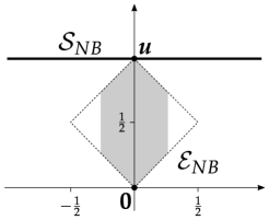
Figure 3 shows two modified versions of the bit GPT system that violate the no-restriction hypothesis, one of which is a NU GPT system while the other is not. Further examples of the three different varieties of GPT system—restricted, unrestricted and noisy unrestricted—can be found in Section 5.
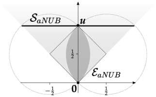
3.3 Almost noisy unrestricted GPTs
We now introduce almost NU GPTs as a relaxation of the class of NU GPTs. Just as a NU GPT, a given almost NU GPT will be related to a unique unrestricted GPT. However, given an observable of the unrestricted GPT, it will be sufficient for the almost NU GPT to include a noisy measurement of an observable arbitrarily close to . In NU GPTs, there is a noisy measurement for each such observable, , so the requirement is met. In a non-NU GPT it can only be met if the GPT has extremal effects arbitrarily close to the zero effect. For example, consider the almost NU bit depicted in Fig. 4. Every point on the boundary of the effect space is extremal and as the non-zero extremal effects approach zero they also approach the boundary of , the positive cone of the unrestricted bit effect space.
In general an almost NU GPT is defined as follows.
Definition 4.
A GPT system is almost noisy unrestricted (aNU) whenever its state space and effect space satisfy the following condition: for every vector and every there exists a vector and a number such that and the rescaled vector is contained in the effect space .
Alternatively, we can characterise aNU GPTs as those that can simulate any observable in their unrestricted counterpart arbitrarily well via post-selection. Explicity, for every observable in the unrestricted GPT system and , there exists a second observable (the approximation) of the unrestricted GPT system satisfying for all , and also a probability such that is an observable of the aNU GPT system. The fact that Def. 4 is a necessary condition for a GPT to have this property is clear. To show that it is also sufficient we need the following alternative characterisation of aNU GPTs which will also be key to proving our main result.
Lemma 5.
In an almost NU GPT the state space and effect space of each system are related by .
The proof can be found in Appendix A. Note that, as shown in the proof of Lemma 5, in an aNU GPT we find , a condition considered by Ludwig in his operational framework, see [26, Chapt. VI, Thm. 2.2.1].
Now we can show that an aNU GPT system contains an observable which is a noisy version of an arbitrarily close approximation to any observable in its unrestricted counterpart. Let and be state and effect spaces of a system in an almost NU GPT and be the effect space of the corresponding unrestricted GPT system. Firstly, if we may take . Secondly, for every in the unrestricted system and define where
for all . Since spans and contains for all it follows that and hence are interior points of . By the equality we have that and thus the observable
is in the aNU GPT for some . This observable is a noisy version of the observable which satisfies for all .
Note that, compared to the condition in Lemma 5, NU GPTs satisfy the stronger condition . Hence in GPTs which are aNU but not NU we find , i.e. the positive cones of the effect spaces are not closed. It follows from the proof of Lemma 4 that only holds when there are extremal effects arbitrarily close to the zero effect, such as in the aNU bit in Fig. 4.
4 Gleason-type theorems for GPTs
Gleason’s theorem is motivated by the idea the probabilities of the outcomes of any measurement performed on a quantum system should uniquely define the state of the system. Thus, every state should come with a frame function, that is a probability assignment on the space of projections (and later, quantum effects [3]) such that the probabilities of the disjoint outcomes of any measurement sum to unity. In order to formulate a GTT for GPTs, we need to generalize the concept of a frame function.
Definition 5.
A frame function on the effect space of a GPT system is a map satisfying
-
(V1)
for all effects ;
-
(V2)
for all sequences of effects such that is an observable in the GPT.
Considering measurements with only a finite number of possible outcomes is sufficient for our purposes; thus, assumption (V2) is only required to hold for finite sequences of effects. Countable sequences of effects may be required if one considers infinite-dimensional systems.
In quantum theory the results of Gleason and Busch show that any frame function must correspond to a density operator. In other words, there are no states beyond those we already believe to exist under the assumption that states must correspond to frame functions. We will take the analog of this idea as the definition of a GTT for a GPT.
Definition 6.
A GPT admits a Gleason-type theorem if and only if for each of its systems every frame function on the effect space can be represented by a state in the state space .
In this definition, the state space is prescribed by the GPT and may be a subset of the set of all mathematically well-defined states given the effect space . The existence of a GTT would allow the set of all possible states of a GPT system to follow from the effect space via the natural assumption that a state can be uniquely defined by its propensity to take each possible value of every observable. The requirement that all mathematically possible states are realised in a theory could be thought of as dual to the no-restriction hypothesis, i.e. requiring that all effects have a corresponding measurement outcome. We will show, however, that the classes of GPTs that satisfy these requirements do not coincide.
4.1 A Gleason-type theorem for almost NU GPTs
After these preliminaries, let us state the main result of this paper which identifies the condition under which Gleason-type theorems exist for general probabilistic theories.
Theorem 1.
Let and be the state and effect spaces, respectively, of a GPT system. Any frame function admits an expression for some if and only if
| (20) |
i.e. a GPT admits a Gleason-type theorem if and only if it is an almost noisy unrestricted GPT.
4.2 Consequences of a GTT for aNU GPTs
Before presenting the proof of Theorem 1, we briefly explain how a GTT allows one to simplify the postulates used to describe a specific GPT in an axiomatic approach. A simple way to state the postulates, often used for quantum theory, is to describe the mathematical objects that represent observables and states along with the rule for calculating the probabilities of measurement outcomes (supplemented by postulates describing the composition of systems and, possibly, the evolution of the system in time). In general, for some GPT system with effect space and state space , such postulates would take the following form:
-
(O)
The observables of the system correspond exactly to the tuples of vectors in that sum to the vector , with each vector corresponding to a possible disjoint outcome of measuring the observable.
-
(S)
The states of the system correspond exactly to vectors .
-
(P)
When measuring the observable on a system in state , the probability to obtain outcome is given by .
If there exists a GTT for the GPT in hand, then it could be recovered by replacing the postulates (S) and (P) by the operationally motivated assumption that every state must have a corresponding frame function defining its outcome probabilities, along with the converse assumption that every frame function must have a corresponding state in the theory. Consequently, one only needs to supplement postulate (O) with a single new postulate.
-
(F)
There exists a state of the system for every frame function on the effect space .
Combined with the GTT and operational reasoning, postulates (O) and (F) lead to the same theory as the postulates (O), (S) and (P). Thus, the Gleason-type theorem would simplify the axiomatic formulation of the GPT, just as the theorems by Gleason or Busch do in the case of quantum theory.
It could be argued that the operational assumptions present in the derivation of the GPT framework are better suited to simplifying the postulates (O), (S) and (P). In Appendix B we compare this strategy with the simplification achieved using Theorem 1.
Our result also opens up an alternative step in establishing the GPT framework. In Section 2 we reviewed the derivation of the framework from operational principles which motivates the structure of state spaces in GPTs from the assumption of fiducial measurement outcomes, as in [9, 6, 7, 27, 21, 28]. The approach then arrives at the effect-space structure by motivating effects as affine functions on the states space.
One may, however, invert this process and arrive at the same framework. By assuming that fiducial states exist one can motivate the structure of effect spaces in GPTs444The approach of motivating the structure of measurements first features in other formalisms; for example, see Ludwig’s work on operational theories, summarised in [26], or the theory of test-spaces and its predecessors [29, 30, 31]., namely as convex, compact subsets of a real vector space containing the zero vector and a vector such that is in the set for every effect 555This structure predates the GPT framework, see [26, Chapt. IV, Thm. 1.2].. At this point, the standard approach would motivate states as affine functionals on the effect space using arguments based on classical mixtures.
Our results offer a mathematically weaker alternative: it is sufficient to combine the effect-space structure with a minimal set of two-outcome observables and their convex combinations as described in Section 6. Then, a corollary to our Gleason-type theorem may be used to recover the structure of the state space (as a subset of where is the effect space of the model) from the assumption that a state must come with a unique frame function on this minimal set of observables.
In other words, assuming that states are frame functions offers an alternative to the mathematically stronger assumption that states are linear functionals on the real vector space containing the effect space. The details of this approach are described in Appendix C.
We highlight one observation following from this derivation, namely, the inequivalence of the no-restriction hypothesis—as described in Section. 3.1—and the dual assumption in the fiducial-states approach, which we will call the no-state-restriction hypothesis666Following this terminology the no-restriction hypothesis should be more accurately called the no-effect-restriction hypothesis. For consistency with the literature and brevity we will stick with with the standard nomenclature.. Recall that the no-restriction hypothesis assumes that, given a state space , every mathematically valid effect is indeed an effect of the system, i.e. . The no-state-restriction hypothesis says that, given an effect space , every mathematically valid state appears in the theory, i.e. . As shown in the proof of Theorem 1 below, the relation holds for exactly almost NU GPTs. Therefore we can conclude that the no-restriction and no-state-restriction hypotheses are not equivalent and the former constitutes a stronger assumption.
Since both approaches are operationally valid, the no-restriction hypothesis and the no-state-restriction hypothesis appear to be motivated equally well. One could argue that their inequivalence demonstrates that neither assumption is valid. In any case, if one is ready to assume either of them, one should be willing to assume the other, too. Thus, the stronger no-effect-restriction hypothesis should be taken, as seems to have happened naturally in the literature, e.g in [6, 27, 32, 33, 19]. Conversely, they should also both be rejected together, meaning no-go theorems such as in [28] would benefit from targetting the weaker no-state-restriction hypothesis.
4.3 Proof of Theorem 1
Using Definition 6 of a GTT, Theorem 1 shows that aNU GPTs are exactly the class of GPTs that admit GTTs. We will prove this result in two steps: (i) in Lemma 6, a frame function on a GPT effect space is found to correspond to a vector in the set defined in Section 3.1; (ii) the set is found to correspond to the state space of a GPT system if and only if the GPT is in the class of aNU GPTs, in Lemmata 7 and 8.
Step (i): The proof of the following lemma777This lemma was independently shown in [34], where it is considered as a GTT for GPTs. follows the one for the quantum case given in [3].
Lemma 6.
Let be an effect space of a GPT. Any frame function on admits an expression
| (21) |
for some vector and all effects .
Lemma 6 shows that if one defines states as frame functions on an effect space , then the associated state space must be .
Step (ii): We will now prove that the set corresponds to the state space of a GPT system with effect space if and only if the GPT is an aNU GPT. Two lemmata will be needed to show that holds for all GPTs while the relation only holds for aNU GPTs. The proofs can be found in Appendix D.
Lemma 7.
For any GPT system with state space , we have .
Lemma 8.
Given a GPT system with state and effect spaces and , respectively, the relation holds if and only if .
We are now in a position to prove our main result, Theorem 1, announced in the previous section. It states that a general probabilistic theory admits a Gleason-type theorem if and only if it is almost noisy unrestricted. The result is an immediate consequence of the lemmata just shown.
5 Examples and applications
In this section, we will consider examples of NU GPT systems to show how their axiomatic formulation simplifies due to the Gleason-type theorem they allow. We also highlight that a simple well-known non-quantum model introduced by Spekkens [35] does not belong to the class of almost NU GPTs and, therefore, does not come with a GTT.
5.1 Simplified axioms for a rebit and other unrestricted GPTs
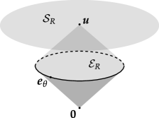
Unrestricted GPTs are a well-studied class of GPT. The rebit [14], for example, is a GPT system with a disc-shaped state space. The state space can be equivalently modeled (see Section 2.3) by the subset of real density matrices of a qubit. Rebits are convenient low-dimensional building blocks for a toy model of quantum theory, giving rise to many characteristic features such as superposition, entanglement and non-locality [16, 14, 32].
Using our notation, the state space of a rebit is given by
| (25) |
where
| (26) |
The convex hull of the zero effect , the unit effect and a continuous ring of effects
| (27) |
form the rebit effect space
| (28) |
illustrated in Figure 5a. The rebit satisfies the no-restriction hypothesis since the effect space is as large as is permitted in the GPT framework (see Eq. 17).
Let us now apply the general argument given at the end of Section 4.1 to a rebit, as a first example of an unrestricted GPT. Instead of using the GPT framework, we could have described the rebit of this hypothetical world in an axiomatic fashion, i.e. by assuming the axioms (O), (S) and (P) from Section 4.1, using the effect and state spaces and . Then, Theorem 1 states that, alternatively, we could postulate the rebit observables and, by considering the frame functions associated with them, recover both the state space and the probability rule. More explicitly, we replace postulates (S) and (P) by a single postulate with operational motivation.
-
(F)
The states of a rebit correspond exactly to the frame functions on the effect space .
In other words, we effectively introduce the states of the rebit as probability assignments on the outcomes of measurements. The model created by the postulates (O) and (F) is equivalent to the the original one in the sense that it makes exactly the same predictions.
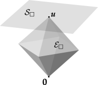
Classical bits, qubits and qudits as well as square bits (or squits, for short) are other unrestricted GPTs for which identical arguments also result in a smaller set of axioms by means of our Gleason-type theorem. The state and effect spaces of bits and qudits were described in Section 2.3 while a squit or gbit [6] is a GPT with a square state space and an octahedral effect space, as illustrated in Figure 5b. Pairs of squits are often considered in the study of non-local correlations since they are capable of producing the super-quantum correlations of a PR-box [36].
5.2 A GPT with a GTT: the noisy rebit
Next, let us consider a noisy rebit characterized by the property that the extremal rebit observables can be measured only imperfectly, i.e. with some efficiency ; see Eq. (27) for the definition of the effects 888The noisy rebit GPT also results from applying the general (shifted) depolarizing channel for a generic state to the rebit effect space; see [20] for details of the analogous qubit case.. The state space of this NU GPT system coincides with that of the rebit, . In order to define its effect space , let us introduce two continuous rings of effects,
| (29) |
These rings, along with the zero effect and the unit effect , form the extremal points of the noisy rebit effect space,
| (30) |
depicted in Figure 6. While still being a GPT system, the model does not satisfy the no-restriction hypothesis: the effect space is restricted to a proper subset of shown in Figure 5a. Nevertheless, Theorem 1 continues to apply: the noisy rebit admits a GTT which is effectively due to the fact that there exist finite neighbourhoods of the zero effect and the unit effect in which and coincide. Thus, the noisy rebit does not satisfy the no-restriction hypothesis, but it does satisfy the dual assumption of the no-state-restriction hypothesis (see Appendix C).
Repeating the argument presented in Section 5.1, we are able to simplify the definition of the noisy rebit in terms of postulates (O), (S), and (P) which introduce its effect space , its state space , and the Born rule, respectively. The alternative axiomatic formulation in terms of only two postulates only rests on the effect space of the system,
-
(O)
The observables of a noisy rebit correspond exactly to the tuples of vectors in that sum to the vector , with each vector corresponding to a possible disjoint outcome of measuring the observable.
-
(F)
The states of a noisy rebit correspond exactly to frame functions on the effect space .
Mutatis mutandis, this procedure applies to any other aNU GPT.
5.3 A GPT without a GTT: the Spekkens toy model
In 2007, a toy theory was introduced [35] capable of reproducing a number of important quantum features such as the existence of non-commuting observables, the impossibility of cloning arbitrary states and the presence of entanglement while simultaneously admitting a description in terms of local hidden variables. Originally, Spekkens’ model had been introduced without reference to the GPT framework. Here, we will consider the “convexification” of this model such that it becomes a GPT system, as described in [11].
Considered as a GPT system, Spekkens’ model comes with a restricted effect space, and it is not part of an aNU GPT which can be seen as follows. Its state space is given by a regular octahedron
| (31) |
with vertices
| (32) |
Under the no-restriction hypothesis the extremal effects (other than the zero and unit effects) associated with the space would be the vertices of a cube. In Spekkens’ model, however, they are taken to be the vertices of another octahedron inscribed into this cube, as depicted in Figure 7. More explicitly, the effect space is the convex hull of the zero and unit effects and the six extremal effects given by the (rescaled) vectors in Eq. (32),
| (33) |
Not being an aNU GPT system, Theorem 1 tells us that the toy model does not admit a GTT.999This fact was, of course, clear without Theorem 1 since every vector in yields frame function by definition. It is impossible to reproduce this GPT system by assuming that the states of the system are in one-to-one correspondence with the frame functions on the effect space. There are, in fact, more frame functions than states in . The frame functions correspond to all vectors in the set which is a strict superset of forming a cube around , in the same way that encloses in Figure 7.
In order to recover the original model, one would have to place a restriction on which frame functions correspond to allowed states. This restriction can be considered analogous to relaxing the no-restriction hypothesis on the effect space.

6 A GTT for almost NU GPTs based on two-outcome observables
The definition of a frame function used in Section 4 is based on the idea that every sequence of effects satisfying Eqs. (7) and (8) corresponds to an observable. This assumption is, however, not operationally motivated and is therefore not part of the most general GPT framework. In this section we show that relaxing this assumption does not pose an obstacle to the existence of Gleason-type theorems. In quantum theory a Gleason-type theorem can already be derived by involving only a specific subset of all POMs [37] known as projective-simulable observables [38]. We will show now that a similar weakening of the assumptions continues to imply the result of Theorem 1 in the context of GPTs. In this way, we are able to extend our result to the most general type of GPTs.
Let us begin by introducing the idea of simulating the measurement of an observable by measuring other observables. This simulation is achieved in a GPT by classically mixing observables and post-processing measurement outcomes [39]. For example, to simulate the observable
| (34) |
we may measure the observables
| (35) |
with probabilities and and , respectively, to simulate
| (36) |
followed by coarse-graining the first two outcomes to produce the dichotomic observable , where the addition and scalar multiplication of observables is performed elementwise. The only post-processing necessary in the proof to follow is to add outcomes to an observable that occur with probability zero. For example, the two-outcome observable simulates the three-outcome observable if one considers there to be a third outcome of measuring which never occurs.
Now consider the set of observables which may be simulated by two-outcome extremal observables, i.e. those described by an extremal effect and its complement . For brevity we will refer to such observables as simulable. We now define simulable observables, denoting by the -th outcome of an observable . A dichotomic observable has precisely two non-zero effects and, possibly, any number of copies of the zero effect.
Definition 7.
A simulable -outcome observable satisfies
for some probability distribution such that for and some classical mixture of dichotomic extremal observables.
The set of simulable observables is minimal in the sense that it is contained in any set of observables, under the operational assumption that a set of observables be simulation-closed [20]. To see this we first note that each extremal effect must be included in some observable, otherwise it would be excluded from the effect space. Any observable containing a given extremal effect can be coarse-grained to give the two-outcome extremal observable . Thus, in order to be closed under simulation a set of observables must at least contain all those that can be simulated by two-outcome extremal observables.
Next, let us call a frame function simulable if the property (V2) in Definition 5 is required to hold for simulable observables only.
Definition 8.
A simulable frame function on an effect space is a map satisfying
-
(S1)
for all effects ;
-
(S2)
for all sequences of effects which give rise to simulable observables .
Theorem 1 can now be strengthened because the properties of simulable frame functions are sufficient for a proof.
Theorem 2.
Let and be the state and effect spaces, respectively, of a NU GPT. Any simulable frame function on admits an expression
| (37) |
for some and all .
Proof.
See Appendix E. ∎
7 Summary and Discussion
From a conceptual point of view, the results of this paper imply that each general probabilistic theory belongs to one of two distinct classes: either it admits, like quantum theory, a Gleason-type theorem which allows us to construct the set of the possible states of the theory, or it does not admit a GTT.
In Lemma 6 (see Section 4) frame functions were found to be linear functionals on the effect space. If one considers this fact to be the main content of the Gleason-type theorems in quantum theory then the lemma proves that Gleason-type theorems exist for all GPTs. In this paper we have, however, taken the view that a Gleason-type theorem should establish a bijection between frame functions and states in the theory under consideration.
Interpreting GTTs in this way, Theorem 1 shows that a GPT admits such a theorem if and only if it is an almost noisy unrestricted GPT, of which classical and quantum models are examples. Requiring that there is a state in a theory for every frame function could be considered as dual to the no-restriction hypothesis which demands that to every mathematical effect there should correspond a measurement outcome. However, we have shown that the no-restriction hypothesis is more restrictive than requiring the existence of a GTT. On the one hand, every unrestricted GPT admits a GTT but, on the other, there are almost NU GPTs that admit a GTT but violate the no-restriction hypothesis. Phrased differently, the no-effect-restriction hypothesis is manifestly different from the no-state-restriction hypothesis.
In Section 4.1 we describe how a Gleason-type theorem can be used to derive the state space in a given GPT from the set of observables. The postulates (O), (S) and (P), which specify a given GPT, can be replaced by just two postulates, namely (O) and (F), when the description of states as frame functions is assumed. This reduction is only possible in almost NU GPTs.
Extensions of Gleason’s theorem to beyond quantum theory have been considered previously in the literature. Gudder et al. [12] consider states on convex effect algebras. These algebras can be represented [40] by subsets of a real linear space in which is a positive cone and is an element of . This representation coincides with unrestricted effect spaces in our terminology. Morphisms (which coincide with frame functions in our terminology) were shown in [12] to extend to positive linear functionals on . Barnum [41] pointed out that this result can be considered as a Gleason-type theorem demonstrating, in our terminology, the existence of a Gleason-type theorem for unrestricted GPTs. Theorem 1 extends this result to exactly the class of almost NU GPTs.
In recent work [42, 43, 44], alternatives to simplifying the postulates of quantum theory have been put forward by assuming, for example, the postulates of pure states and their dynamics in combination with operational reasoning. It would be interesting to study whether similar approaches also hold for other GPTs, or whether they are unique to quantum theory.
The current work relies heavily on the convex structure of GPTs. In future work we would like to establish which GPTs admit an analog of Gleason’s original theorem, in the sense that the frame functions would only be defined on extremal effects where convexity arguments can no longer be made.
Finally, it might be possible to establish a link between Gleason-type theorems and the set of almost-quantum correlations [45]. It is known that GPTs satisfying the no-restriction hypothesis cannot produce the set of almost quantum correlations in Bell scenarios [28]. If this result could be extended to almost NU GPTs then the existence of a GTT for a GPT would also preclude the possibility of that GPT producing the set of almost quantum correlations.
Acknowledgement.
We are grateful to an anonymous referee for pointing out a mistake in a draft of our manuscript and for suggesting a way to correct it which triggered the extension of the result from NU GPTs to aNU GPTs. VJW acknowledges support by the Foundation for Polish Science (IRAP project, ICTQT, contract no. 2018/MAB/5, co-financed by EU within Smart Growth Operational Programme) and the Government of Spain (FIS2020-TRANQI and Severo Ochoa CEX2019-000910-S), Fundació Cellex, Fundació Mir-Puig, Generalitat de Catalunya (CERCA, AGAUR SGR 1381 and QuantumCAT).
References
- [1] George W Mackey. Quantum mechanics and Hilbert space. Am. Math. Mon., 64:45–57, 1957. doi:10.2307/2308516.
- [2] Andrew M Gleason. Measures on the closed subspaces of a Hilbert space. J. Math. Mech., 6:885, 1957. doi:10.1007/978-94-010-1795-4_7.
- [3] Paul Busch. Quantum states and generalized observables: a simple proof of Gleason’s theorem. Phys. Rev. Lett., 91:120403, 2003. doi:10.1103/physrevlett.91.120403.
- [4] Carlton M Caves, Christopher A Fuchs, Kiran K Manne, and Joseph M Renes. Gleason-type derivations of the quantum probability rule for generalized measurements. Found. Phys., 34:193–209, 2004. doi:10.1023/b:foop.0000019581.00318.a5.
- [5] Peter Janotta and Haye Hinrichsen. Generalized probability theories: what determines the structure of quantum theory? J. Phys. A, 47:323001, 2014. doi:10.1088/1751-8113/47/32/323001.
- [6] Jonathan Barrett. Information processing in generalized probabilistic theories. Phys. Rev. A, 75:032304, 2007. doi:10.1103/PhysRevA.75.032304.
- [7] Lluís Masanes and Markus P Müller. A derivation of quantum theory from physical requirements. New J. Phys., 13:063001, 2011. doi:10.1088/1367-2630/13/6/063001.
- [8] Howard Barnum and Alexander Wilce. Information processing in convex operational theories. Electron. Notes Theor. Comput. Sci., 270(1):3–15, 2011. doi:10.1016/j.entcs.2011.01.002.
- [9] Lucien Hardy. Quantum theory from five reasonable axioms. arXiv:quant-ph/0101012, 308, 2001. URL: https://arxiv.org/abs/quant-ph/0101012.
- [10] Giulio Chiribella, Giacomo Mauro D’Ariano, and Paolo Perinotti. Probabilistic theories with purification. Phys. Rev. A, 81:062348, 2010. doi:10.1103/PhysRevA.81.062348.
- [11] Peter Janotta and Raymond Lal. Generalized probabilistic theories without the no-restriction hypothesis. Phys. Rev. A, 87:052131, 2013. doi:10.1103/PhysRevA.87.052131.
- [12] Stanley P Gudder, Sylvia Pulmannová, Sławomir Bugajski, and Enrico Beltrametti. Convex and linear effect algebras. Rep. Math. Phys., 44(3):359–379, 1999. doi:10.1016/s0034-4877(00)87245-6.
- [13] Michał Oszmaniec, Filip B. Maciejewski, and Zbigniew Puchała. Simulating all quantum measurements using only projective measurements and postselection. Phys. Rev. A, 100:012351, 2019. doi:10.1103/PhysRevA.100.012351.
- [14] Carlton M Caves, Christopher A Fuchs, and Pranaw Rungta. Entanglement of formation of an arbitrary state of two rebits. Found. Phys. Lett., 14(3):199–212, 2001. doi:10.1023/A:1012215309321.
- [15] Lucien Hardy and William K Wootters. Limited holism and real-vector-space quantum theory. Found. Phys., 42(3):454–473, 2012. doi:10.1007/s10701-011-9616-6.
- [16] William K Wootters. Entanglement sharing in real-vector-space quantum theory. Found. Phys., 42(1):19–28, 2012. doi:10.1007/s10701-010-9488-1.
- [17] Antoniya Aleksandrova, Victoria Borish, and William K Wootters. Real-vector-space quantum theory with a universal quantum bit. Phys. Rev. A, 87(5):052106, 2013. doi:10.1103/physreva.87.052106.
- [18] Koji Nuida, Gen Kimura, and Takayuki Miyadera. Optimal observables for minimum-error state discrimination in general probabilistic theories. J. Math. Phys., 51(9):093505, 2010. doi:10.1063/1.3479008.
- [19] Ludovico Lami, Bartosz Regula, Ryuji Takagi, and Giovanni Ferrari. Framework for resource quantification in infinite-dimensional general probabilistic theories. Phys. Rev. A, 103(3), 2021. doi:10.1103/physreva.103.032424.
- [20] Sergey N Filippov, Stan Gudder, Teiko Heinosaari, and Leevi Leppäjärvi. Operational restrictions in general probabilistic theories. Found. Phys., 50(8):850, 2020. doi:10.1007/s10701-020-00352-6.
- [21] Howard Barnum, Markus P Müller, and Cozmin Ududec. Higher-order interference and single-system postulates characterizing quantum theory. New J. Phys., 16(12):123029, 2014. doi:10.1088/1367-2630/16/12/123029.
- [22] Gen Kimura. The Bloch vector for N-level systems. Phys. Lett. A, 314:339–349, 2003. doi:10.1016/s0375-9601(03)00941-1.
- [23] Sandeep K Goyal, B Neethi Simon, Rajeev Singh, and Sudhavathani Simon. Geometry of the generalized Bloch sphere for qutrits. J. Phys. A, 49(16):165203, 2016. doi:10.1088/1751-8113/49/16/165203.
- [24] Ingemar Bengtsson and Karol Życzkowski. Geometry of quantum states: an introduction to quantum entanglement. Cambridge University Press, 2017. doi:10.1017/9781139207010.
- [25] R Tyrrell Rockafellar. Convex analysis. Princeton University Press, 1970. doi:10.1515/9781400873173.
- [26] Günther Ludwig. An Axiomatic Basis for Quantum Mechanics. Volume 1: Derivation of Hilbert Space Structure. Springer, 1985. doi:10.1007/978-3-642-70029-3.
- [27] Anthony J Short and Jonathan Barrett. Strong nonlocality: a trade-off between states and measurements. New Journal of Physics, 12(3):033034, 2010. doi:10.1088/1367-2630/12/3/033034.
- [28] Ana Belén Sainz, Yelena Guryanova, Antonio Acín, and Miguel Navascués. Almost-quantum correlations violate the no-restriction hypothesis. Phys. Rev. Lett., 120(20):200402, 2018. doi:10.1103/physrevlett.120.200402.
- [29] David J Foulis and Charles H Randall. Empirical logic and tensor products. In Interpretations and foundations of quantum mechanics: proceedings of a conference hold in Marburg 28-30 May 1979. 1981. URL: https://inis.iaea.org/search/search.aspx?orig_q=RN:13651556.
- [30] Charles H Randall and David J Foulis. Operational statistics. ii. manuals of operations and their logics. J. Math. Phys., 14:1472–1480, 1973. doi:10.1063/1.1666208.
- [31] David J Foulis, Richard J Greechie, and Gottfried T Rüttimann. Logicoalgebraic structures II. Supports in test spaces. Int. J. Theor. Phys., 32(10):1675–1690, 1993. doi:10.1007/bf00979494.
- [32] Peter Janotta, Christian Gogolin, Jonathan Barrett, and Nicolas Brunner. Limits on nonlocal correlations from the structure of the local state space. New J. Phys., 13(6):063024, 2011. doi:10.1088/1367-2630/13/6/063024.
- [33] Ludovico Lami. Non-classical correlations in quantum mechanics and beyond. PhD thesis, Universitat Autònoma de Barcelona, arXiv:1803.02902, 2017. URL: https://arxiv.org/abs/1803.02902.
- [34] Farid Shahandeh. Contextuality of general probabilistic theories. PRX Quantum, 2(1):010330, 2021. doi:10.1103/prxquantum.2.010330.
- [35] Robert W Spekkens. Evidence for the epistemic view of quantum states: A toy theory. Phys. Rev. A, 75(3):032110, 2007. doi:10.1103/physreva.75.032110.
- [36] Sandu Popescu and Daniel Rohrlich. Quantum nonlocality as an axiom. Found. Phys., 24(3):379–385, 1994. doi:10.1007/bf02058098.
- [37] Victoria J Wright and Stefan Weigert. A Gleason-type theorem for qubits based on mixtures of projective measurements. J. Phys. A, 52:055301, 2019. doi:10.1088/1751-8121/aaf93d.
- [38] Michał Oszmaniec, Leonardo Guerini, Peter Wittek, and Antonio Acín. Simulating positive-operator-valued measures with projective measurements. Phys. Rev. Lett., 119(19):190501, 2017. doi:10.1103/physrevlett.119.190501.
- [39] Sergey N Filippov, Teiko Heinosaari, and Leevi Leppäjärvi. Simulability of observables in general probabilistic theories. Phys. Rev. A, 97:062102, 2018. doi:10.1103/PhysRevA.97.062102.
- [40] Stanley P Gudder and Sylvia Pulmannová. Representation theorem for convex effect algebras. Comment. Math. Univ. Carolinae, 39(4):645–659, 1998. URL: https://dml.cz/handle/10338.dmlcz/119041.
- [41] Howard Barnum. Quantum information processing, operational quantum logic, convexity, and the foundations of physics. Stud. Hist. Philos. Sci. A, 34(3):343–379, 2003. doi:10.1016/s1355-2198(03)00033-9.
- [42] Lluís Masanes, Thomas D Galley, and Markus P Müller. The measurement postulates of quantum mechanics are operationally redundant. Nat. Commun., 10(1):1–6, 2019. doi:10.1038/s41467-019-09348-x.
- [43] Thomas D Galley and Lluís Masanes. Classification of all alternatives to the Born rule in terms of informational properties. Quantum, 1:15, 2017. doi:10.22331/q-2017-07-14-15.
- [44] Thomas D Galley and Lluís Masanes. Any modification of the Born rule leads to a violation of the purification and local tomography principles. Quantum, 2:104, 2018. doi:10.22331/q-2018-11-06-104.
- [45] Miguel Navascués, Yelena Guryanova, Matty J Hoban, and Antonio Acín. Almost quantum correlations. Nat. Commun., 6(1):1–7, 2015. doi:10.1038/ncomms7288.
- [46] Lucien Hardy. Disentangling nonlocality and teleportation. arXiv:quant-ph/9906123, 1999. URL: https://arxiv.org/abs/quant-ph/9906123.
Appendix A Proofs of Lemmata 2, 3 , 4 and 5
See 2
Proof.
Firstly, let . Then there exists a sequence such that as with . For any we have and, since the inner product is continuous, . Therefore we have shown .
Secondly, consider . By the hyperplane separation theorem there exists and real numbers such that for all and . For all and we have and therefore . Taking the limit as we find for all and hence . Finally, since we find , and thus , meaning since we found that . ∎
See 3
Proof.
By Definition 2, a vector is in the dual cone of if and only if for all . Equivalently, we may require for all vectors in the set and which holds if and only if . ∎
See 4
Proof.
Firstly, note that by definition the set does not contain the zero vector, . Let be a convergent sequence in such that for all and as . We will show that .
If , the statement holds. Now assume . For each there exists and such that . By the Bolzano-Weierstrass theorem and the compactness of , the sequence has a convergent subsequence such that as .
Now we show that the corresponding subsequence neither diverges to infinity nor tends to zero. Firstly, assume that as . Then, since , we find the contradiction . Secondly, assume that as . Then , contradicting our assumption that .
Therefore, since converges, we find there exists a finite number such that as . This result means that in the limit of , will converge to an element of : as . ∎
See 5
Proof.
Consider a GPT system with state space and effect space . Assume that the spaces satisfy .
Then if , we have and for every there exists such that . Hence there exists such that which means that the GPT system satisfies Definition 4.
Conversely, assume that the GPT satisfies Definition 4. We will show that , by firstly showing and secondly that .
For every vector (where and ) and there exists (where and ) such that . Letting , we find for every and there exists such that . Since every point in is a point of closure of we find .
To prove that , we begin by showing that is a closed set. Firstly, we have by Eq. (17). Then we find
| (38) |
as follows. The set on the left of this equation is clearly contained in that on the right since we have . Furthermore, if , then non-negative rescalings of are also contained in : for all . Since for all , is an internal point of . Thus, there exists an open ball around of radius in for some . Therefore, for we have and hence . By definition, , hence we have and , thus verifying Eq. (38). The dual cone is, by definition, the intersection of a collection of closed halfspaces therefore is closed.
Now, since is closed and contains , we have . Finally, we have shown which gives . ∎
Appendix B An alternative simplification of the axioms defining a GPT
Let us briefly mention an alternative approach to simplifying the postulates (S), (O) and (P) providing an equivalent definition a GPT which closely follows the operational assumptions of the GPT framework. It should be compared with the simplification using Theorem 1 outlined at the end of Section 4.1. The starting point is a single postulate about the states of the model at hand.
-
(S’)
There exist fiducial measurement outcomes of observables whose probabilities determine the state of the system. These states are restricted to being represented by vectors in .
The first part of the postulate, the existence of fiducial measurement outcomes, determines that the state space can be embedded in and is convex, with convex combinations of vectors representing classical mixtures of the corresponding states. However, this assumption does not determine the “shape” of the state space, hence the inclusion of the second part of the postulate restricting the state space to . For a specific GPT, the second part of the postulate may take a more natural-sounding form such as state vectors having modulus less than or equal to one. From (S’), using the standard operational assumption that effects must respect classical mixtures and the no-restriction hypothesis (see Section 2), the postulates (O) and (P) are recovered easily.
Let us conclude by comparing this approach to our approach of using Theorem 1 in order to reduce the postulates (O), (S) and (P).
First, postulate (O) does not assume that there exists fiducial outcomes. This property is a consequence in our approach once the states are identified as linear functionals on the effect space. Therefore, postulate (O) is not simply a stronger version of (S’).
Second, in order to postulate the existence of fiducial measurement outcomes, as is done in (S’), one assumes some knowledge of all the observables of the system; otherwise one would not know that the two outcomes in question form a complete fiducial set. Therefore, axiom (S’) makes assumptions about both the states and the observables of the system whereas (O) only concerns observables.
Finally, in the approach based on (S’), additional assumptions would be necessary to reconstruct an almost NU GPT which does not satisfy the no-restriction hypothesis because one could not use the no-restriction hypothesis to recover the postulates (O) and (P). However, such a GPT does admit a GTT, as Theorem 1 shows, and hence the first method would still be valid.
Appendix C The “fiducial state” derivation of the GPT framework
In the modern literature, the GPT framework is typically derived, as in Section 2, by assuming the existence of fiducial measurement outcomes first, then defining the state space of a system, followed by a full treatment of observables and their measurement, see for example [46, 7, 6, 27, 21, 28]. However, one may equally consider the inverted argument, i.e. derive the framework using equivalent operational assumptions, by assuming a fiducial set of states, in order to define all possible measurements and their outcomes then finding the compatible mathematical description of states. Note that such a dual approach is not novel, for example, Ludwig describes the idea in his work on operational theories [26] exemplify and the test-space formalism [29, 31] begins with the structure of measurement outcomes first. Proceeding in this second, dual manner the structure of effect spaces is established first then Theorem 2 presents an alternative method for deriving the structure of state spaces, compared with the standard argument involving mixtures of measurement outcomes.
We begin by summarising the “fiducial states” derivation of the GPT framework in parallel with Section 2. Consider all the possible outcomes of the measurements of all the observables of a given system. We will assume that there exists a finite set of fiducial states such that any one of these outcomes, , is uniquely determined by the probabilities of being observed after a measurement (of which is a possible outcome) is performed on the system in each of the fiducial states. In other words, for a system with states in its fiducial set, an outcome may be identified by the vector such that
| (39) |
where is the probability of observing the outcome for a system in the th fiducial state. This representation of measurement outcomes is derived from the operational assumption that one should be able to distinguish two distinct measurement outcomes by their statistics on a finite number of states, in analogy to assuming the possibility of distinguishing two distinct states from the probabilities of a finite number of measurement outcomes in the “fiducial measurements” approach.
In line with GPT terminology we will call the set of vectors corresponding to outcomes in a model the effect space and the vectors within this set effects. Note that the effects are now simply vectors and not linear functionals. For brevity, we will often refer to a measurement outcome as the effect by which it is represented.
In the bit example from Section 2, the fiducial set of states could be the “0” and “1” states. Thus the effect space would be a subset of .
We will assume the existence of an outcome that occurs with probability one for any state of the system. This outcome must be represented by the effect
| (40) |
Similarly, we assume the existence of an outcome that never occurs, represented by the effect
| (41) |
Any outcome must have a complement, namely the outcome “not ” necessarily occurring with probability when the measurement of “ or not ” is performed on the th fiducial state. Therefore, for any effect the vector
| (42) |
must also be in the effect space.
Consider two measurements on the system each with a discrete set of possible outcomes and label the outcomes of each measurement with positive integers such that the first measurement has outcomes and the second (if the measurement has a finite number, , of possible outcomes the labels for are assigned the zero effect). If a classical mixture of these measurements is performed then possible outcomes of this procedure can be represented by convex combinations of effects. Specifically, if the first measurement is performed with probability and the second with probability , then observing an outcome labeled from this procedure must be represented by the vector in order to be consistent with the fiducial state set. Therefore we assume the effect space is convex. Finally, since an arbitrarily good approximation of an effect would operationally be indistinguishable from the effect itself we assume the effect space is a closed subset of .
Returning to the bit example, we can build our effect space from the requirement of having a measurement that perfectly distinguishes “0” and “1”, and must therefore have outcomes, and . Combined with the other requirements for an effect space we find the bit effect space to be the square in Figure 8, a transformation of the bit effect space described in Section 2.2.
We have arrived at the same requirements for the structure of an effect space as were described in Section 2 (a convex, compact subset of a real vector space containing the zero vector, and a vector such that is in the set for every in the set). We may now consider how states should be represented in the framework. We assume a state will be represented by a map from an outcome to the probability of observing when a measurement (of which is a possible outcome) is performed on a system in state . From here we may derive the state space structure of the GPT framework using the standard operational assumptions or the alternative presented by Theorem 2.
One the one hand, the standard method for deriving the structure of the state space is to exploit the fact that we wish for outcome probabilities to respect mixtures, in analogy with the reasoning behind (5), to find
| (43) |
for and all effects . Thus each map admits an expression
| (44) |
for all effects and some .
One the other hand, we have already assumed that a pair form a measurement and have introduced the formalism for describing mixtures of measurements, therefore the simulable measurements from Section 6 are already included in the framework. Theorem 2 then tells us that if a state is to assign probabilities to the possible outcomes of these measurements such that the probabilities of all the outcomes sum to one then
| (45) |
for all effects and some .
Both of these approaches lead to the conclusion that the state space of a GPT with effect space must be a subset of . Although the conditions are mathematically different there is no clear conceptual advantage to either argument.
The “fiducial states” derivation of the framework highlights the existence of a relative of the no-restriction hypothesis, which we will call the no-state-restriction hypothesis: the inclusion of all satisfying and in the state space. Note that this is not equivalent to the no-restriction hypothesis in all cases, for example the noisy bit model in Figure 3a satisfies the no-state-restriction hypothesis but not the no-restriction hypothesis.
Appendix D Proofs of Lemmata 6, 7 and 8
See 6
Proof.
Consider a finite set of effects such that for any subset . First we show that a frame function must be additive on any such set, i.e.
| (46) |
We have that the tuples
| (47) |
are both observables in the GPT since they satisfy Eqs. (7) and (8). Hence, by property (V2) of a frame function we find
| (48) |
and Eq. (46) follows.
The next step is to show the homogeneity of on , i.e.
| (49) |
Note that the convexity of ensures that rescaling an effect by a factor produces another effect: . For any integer number , Eq. (46) implies
| (50) |
then, letting with , Eqs. (46) and (50) lead to the homogeneity of over the rationals,
| (51) |
Now consider two rational numbers with . Using property (V1) of a frame function with argument guarantees that . Also we find by property (V2) of a frame function that
| (52) |
Thus, the values of frame functions on multiples of a given effect respect the ordering induced by the scale factors,
| (53) |
Next, let and be sequences of rational numbers in the interval that tend to from below and above, respectively. Then we have
| (54) |
so that the homogeneity of claimed in Eq. (49) follows from taking the limit of both sequences.
Thirdly, we construct a well-defined extension of the frame function to , the positive cone associated with (see Definition 1) such that holds for all . To do so, consider two effects which give rise to the same vector in the positive cone via , with . Then we have
| (55) |
hence , and we may uniquely define the frame function on arbitrary vectors in the positive cone by
| (56) |
Additivity of the extended frame function is easily seen to hold for vectors in the positive cone: consider vectors and for and and let . Noting that is an effect, we obtain
| (57) |
A linear extension of a frame function to the whole of follows from the fact that any outside the positive cone may be decomposed into with by Lemma 1. If the decomposition is not unique, , we have leading to
| (58) |
It then follows from Eq. (46), that and hence
| (59) |
Therefore we may uniquely define the value of the frame function on the vector via
| (60) |
i.e. independently of the decomposition of the vector .
This extension of any frame function on to must be linear. First we show additivity: let for , then
| (61) | ||||
Then to show homogeneity let for , firstly consider , in which case we have
| (62) | ||||
Secondly, consider ,
| (63) | ||||
Therefore, the extended map admits an expression as
| (64) |
for some vector , where is a basis of . Finally, requirements (V1) and (V2) on the behaviour of the frame function on the effect space imply that which concludes the proof. ∎
See 7
Proof.
See 8
Appendix E Proof of Theorem 2
Proof.
Due to the convexity of the effect space , we can express any effect as a convex combination , for some extremal effects and real numbers which sum to one. Thus we may simulate the observable
| (74) |
by measuring the observables with probability . Furthermore, for any effects , we may simulate the observable
| (75) |
by performing either or , with equal probability.
Secondly, for any effects such that , the observable
| (78) |
is simulable by Eq. (74). Comparing with Eq. (75) gives
| (79) |
so that follows, using Eq. (77). By induction, any simulable frame function is a frame function as defined in Definition 5. Thus, by Theorem 1, any simulable frame function admits the expression given in Eq. (37). ∎