Non-linear soliton confinement in weakly coupled antiferromagnetic spin chains

Abstract

We analyze the low-energy dynamics of quasi one dimensional, large-$S$ quantum antiferromagnets with easy-axis anisotropy, using a semi-classical non-linear sigma model. The saddle point approximation leads to a sine-Gordon equation which supports soliton solutions. These correspond to the movement of spatially extended domain walls. Long-range magnetic order is a consequence of a weak inter-chain coupling. Below the ordering temperature, the coupling to nearby chains leads to an energy cost associated with the separation of two domain walls. From the kink-antikink two-soliton solution, we compute the effective confinement potential. At distances large compared to the size of the solitons the potential is linear, as expected for point-like domain walls. At small distances the gradual annihilation of the solitons weakens the effective attraction and renders the potential quadratic. From numerically solving the effective one dimensional Schröedinger equation with this non-linear confinement potential we compute the soliton bound state spectrum. We apply the theory to CaFe₂O₄, an anisotropic $S=5/2$ magnet based upon antiferromagnetic zig-zag chains. Using inelastic neutron scattering, we are able to resolve seven discrete energy levels for spectra recorded slightly below the Néel temperature $T_{\textrm{N}}\approx 200$ K. These modes are well described by our non-linear confinement model in the regime of large spatially extended solitons.

I Introduction

Confinement and deconfinement of particles, topological defects or fractionalized excitations are recurring motifs in many areas of physics. A famous example is the quark-gluon plasma, which is predicted to form at extremely high temperatures. In this new state of matter the quarks and gluons, which under normal conditions are strongly confined in atomic nuclei, behave as asymptotically free particlesCollins and Perry (1975). Another example of a confinement-deconfinement transition is the Berenskii-Kosterlitz-Thouless transitionBerezinsky (1971); Kosterlitz and Thouless (1973) in two-dimensional XY magnets that is driven by an unbinding of thermally excited vortex-antivortex pairs.

Spin-charge separation in one dimensionTomonaga (1950); Luttinger (1963); Haldane (1981) can be viewed as a fractionalization of the electrons into holons and spinons, carrying the charge and spin degrees of freedom, respectively. If local repulsions lead to charge localization, the insulating system is well described by the antiferromagnetic $S=1/2$ Heisenberg model. In the presence of Ising exchange anisotropy, spinons can be viewed as domain walls in the antiferromagnetic order and are created in pairs by a single spin flip (see Fig. 1(a)). They are therefore fractionalized excitations that carry half of the spin-1 quantum of a magnon excitation.Faddeev and Takhtajan (1981) If spinons are free to propagate, these pairs are expected to form a triplet excitation continuum. Such continua are predicted theoretically,Bougourzi et al. (1996); Karbach et al. (1997); Caux et al. (2008) building on the analytical Bethe Ansatz solution,Bethe (1931) and observed experimentally in a number of quasi one-dimensional $S=1/2$ antiferromagnets.Mourigal et al. (2013); Bera et al. (2017); Gannon et al. (2019); Wu et al. (2019)

Staggered $g$-tensors and Dzyaloshinskii-Moriya interactions can lead to an unusual field dependence, such as an induced gap,Oshikawa and Affleck (1997); Affleck and Oshikawa (1999) $\Delta\sim H^{2/3}$, and field dependent soft modes at incommensurate wave vectors,Dender et al. (1996, 1997) as predicted by spinon and Bethe Ansatz descriptions.Pytte (1974); Ishimura and Shiba (1977); Müller et al. (1981) Through a procedure of bosonization, the dynamics of such systems can be shown to be governed by the quantum sine-Gordon model which admits soliton and breather solutions, corresponding to propagating and oscillating domain walls, respectively.Affleck and Oshikawa (1999); Essler et al. (2003) This suggests that spinons can be viewed as quantum solitons Lake (2005) and therefore exhibit chirality, which was indeed confirmed by polarized neutron scattering.Braun et al. (2005) Soliton and breather modes were identified in neutron-scattering Kenzelmann et al. (2004); Umegaki et al. (2015) and electron-spin-resonance Zvyagin et al. (2004); Liu et al. (2019) experiments.

The effect of a weak interchain interaction is twofold. Firstly, it sets the temperature scale $T_{\textrm{N}}$ at which two- or three-dimensional long-range order develops. Secondly, it generates an effective attraction between spinons below $T_{\textrm{N}}$ since the separation of domain walls will frustrate interchain interactions with an associated energy cost that grows linearly with their distance. Such a linear confinement potential gives rise to spinon bound states, leading to a quantization of the excitation continuum into discrete energy levels, as observed in BaCo₂V₂O₈,Grenier et al. (2015) SrCo₂V₂O₈,Wang et al. (2015); Bera et al. (2017) and Yb₂Pt₂Pb.Gannon et al. (2019) These systems all consist of weakly coupled Ising-Heisenberg antiferromagnetic (XXZ) chains of $S=1/2$ moments and the measured spinon bound-state energies are almost perfectly described by the eigenvalues of a one-dimensional Schrödinger equation with an attractive linear potential.

Linear confinement due to weak interchain coupling is not specific to spinons in $S=1/2$ quantum antiferromagnets but occurs generically for any type of kink-like domain-wall excitations. In CoNb₂O₆, a quasi one-dimensional Ising ferromagnet, the two-kink continuum breaks up into discrete bound-state excitations below the magnetic ordering temperature, with the same characteristic level spacing as in the spinon case.Coldea et al. (2010)

In this paper we analyze the domain-wall confinement in large-$S$ spin-chain antiferromagnets with easy axis, single-ion anisotropy. Our work is motivated by the observation of discrete energy levels in the anisotropic antiferromagnet CaFe₂O₄,Stock et al. (2016) a spin-5/2 system consisting of weakly-coupled zig-zag chains. As expected for confinement due to frustrated interchain coupling, the bound states form below the the Néel temperature $T_{\textrm{N}}\approx 200$ K. However, the energy levels do not follow the negative zeroes of the Airy function, as predicted for a linear confinement potential.

In the large-$S$ limit, the low-energy effective field theory of the quantum antiferromagnet is the non-linear $\sigma$ model. Starting from this semi-classical description, Haldane demonstrated that the spin dynamics of the one-dimensional quantum antiferromagnet with easy-axis anisotropy is governed by a sine-Gordon equation which supports soliton solutions.Haldane (1983) Hence the domain walls in the antiferromagnetic chain are chiral solitons. In these spin textures the staggered magnetization rotates between the two favored orientations in a clockwise or anti-clockwise direction over a typical distance $\xi$ (see Fig. 1(b)). Since the overall chirality in the system is conserved, the domain walls are created in pairs of soliton (kink, K) and anti-soliton (anti-kink, $\overline{\textrm{K}}$).

Here we compute the confinement potential $V(y)$ from the $\textrm{K}\overline{\textrm{K}}$ two-soliton solution of the sine-Gordon equation and show that the extended nature of semi-classical solitons gives rise to a crossover as a function of the domain-wall separation $|y|$. At large separations, $|y|\gg\xi$, the solitons can be considered as point-like objects, giving rise to a linear confinement potential, $V(y)\sim|y|$. For $|y|<\xi$ the soliton and anti-soliton overlap, leading to a gradual annihilation of the defects and preventing the staggered magnetization between domain walls from fully rotating to the other easy direction. This reduces the interchain-frustration energy, corresponding to a weakening of the effective confinement potential. We find that at small distances, $|y|\ll\xi$, the confinement potential is rendered quadratic, $V(y)\sim y^{2}$.

The bound-state spectrum is obtained from the numerical solutions of a one-dimensional Schrödinger equation with the computed potential $V(y)$. Because of the crossover in $V(y)$, the energies of tightly-bound states are almost equidistant, as expected for a harmonic oscillator, while for the weakly-bound states at higher energies they approach Airy function behavior as predicted for linear confinement.

In order to test our theory, we compare computed spectra to those obtained in inelastic neutron scattering experiments on high-quality single crystals of CaFe₂O₄. Slightly below the Néel ordering temperature, we are able to resolve seven bound states which are well described by our theory of non-linear confinement of spatially extended solitons.

The outline of this paper is as follows. In Sec. II we introduce a generic spin Hamiltonian and resulting low energy, non-linear $\sigma$ model description of a system of weakly coupled antiferromagnetic chains with single-ion Ising anisotropy. We show that the saddle-point approximation results in a sine-Gordon equation and briefly review the one and two-soliton solutions. In Sec. III we compute the energy of a single spin chain with a pair of domain walls from the kink-antikink solution, treating the interchain coupling at mean-field level. The bound state energies are obtained from numerical solutions of the effective Schrödinger equation with the effective non-linear confinement potential. Experimental details and results of our inelastic neutron-scattering experiments on CaFe₂O₄ are presented in Sec. IV. We demonstrate that the measured bound-state energies are well described by our theoretical model. Finally, in Sec. V we summarize and discuss our results.

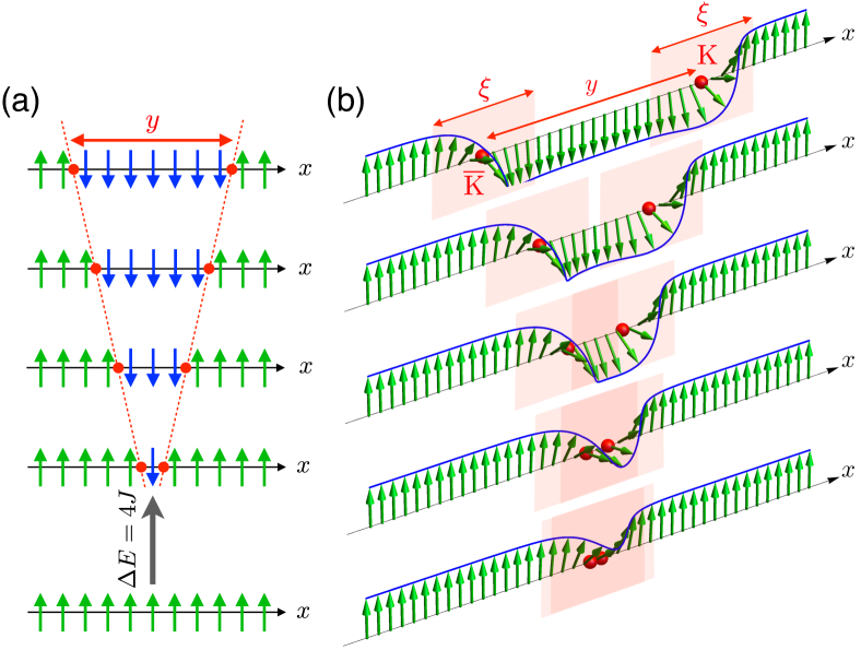
Figure 1: Staggered magnetizations of antiferromagnetic spin chains with Ising anisotropy in the presence of two domain walls (red). (a) For the $S=1/2$ chain, a spin-flip excitation fractionalizes into a pair of spinons. The energy cost due to the coupling to nearby chains scales with the number of spins between the domain walls, giving rise to a linear confinement potential, $V(y)\sim|y|$. (b) For large $S$ spin chains the domain walls are semi-classical chiral solitons of size $\xi$. Shown are different time instances of the collision of a soliton (K) and anti-soliton ($\overline{\textrm{K}}$) obtained from the $\textrm{K}\overline{\textrm{K}}$ two-soliton solution of the sine-Gordon equation. The spatial extent of the domain walls causes them to annihilate gradually, rendering the effective confinement potential quadratic at small distances, $V(y)\sim y^{2}$.

II Theoretical Model

Our starting point is a generic spin model of weakly coupled chains with antiferromagnetic Heisenberg couplings $J$ between nearest neighbor along the chains and $J_{\perp}\ll J$ between the chains. Each spin is subject to a single-ion, easy axis anisotropy $\alpha>0$. The Hamiltonian of the system is given by

$$\hat{\mathcal{H}} = J\sum_{i,m}\hat{\mathbf{S}}_{i,m}\hat{\mathbf{S}}_{i+1,m}-\alpha\sum_{i,m}\left(\hat{S}^{z}_{i,m}\right)^{2}$$ (1)

$$+J_{\perp}\sum_{i,\langle m,n\rangle}\hat{\mathbf{S}}_{i,m}\hat{\mathbf{S}}_{i,n},$$

where $i$ labels the positions in the chains, $m,n$ the different chains, and $\langle m,n\rangle$ denotes nearest neighbor bonds between adjacent chains. In this minimal model, we neglect longer-range exchanges and assume the interchain couplings to be the same in all directions. For simplicity, we have neglected exchange anisotropy between different spin components and Dzyaloshinskii-Moriya interactions. Such terms are not relevant in the case of Calcium Ferrite ($S=5/2$, $L=0$) because of the lack of any orbital degrees of freedom. A discussion of single-ion anisotropy in systems with quenched orbital moment can be found in Ref. [Yosida, 2010].

II.1 Non-linear $\sigma$ model

Let us first focus on an isolated antiferromagnetic chain and drop the chain index for brevity. The effective long-wavelength, non-linear $\sigma$ model is obtained using a path integral in imaginary time $\tau\in[0,\beta]$, $\beta=1/(k_{\textrm{B}}T)$, and resolving the identities between adjacent time slices in terms of over-complete spin-coherent states, $|\mathbf{N}_{i}(\tau)\rangle$. These states are parametrized by unit vectors $\mathbf{N}_{i}(\tau)$ and have the property $\langle\mathbf{N}_{i}(\tau)|\hat{\mathbf{S}}_{i}|\mathbf{N}_{i}(\tau)\rangle=S\mathbf{N}_{i}(\tau)$.

In order to perform a spatial continuum limit, we introduce the staggered Néel order-parameter field $\mathbf{n}_{i}(\tau)$ through the relation $\mathbf{N}_{i}(\tau)=(-1)^{i}\mathbf{n}_{i}(\tau)+a\mathbf{L}_{i}(\tau)$, where $a$ denotes the lattice constant and $\mathbf{L}_{i}(\tau)$ describes the spin fluctuations perpendicular to $\mathbf{n}_{i}(\tau)$. The latter fluctuations are massive and can therefore be integrated out. After taking the continuum limit, this procedure leads to the non-linear $\sigma$ model,Haldane (1983); Sachdev (2011); Fradkin (2013)

$$S=\frac{\rho_{S}}{2}\int_{0}^{\beta}\mathrm{d}\tau\int_{-\infty}^{\infty}\mathrm{d}x\Bigg{\{}\left(\partial_{x}\mathbf{n}\right)^{2}+\frac{1}{c^{2}}\left(\partial_{\tau}\mathbf{n}\right)^{2}-\kappa n_{z}^{2}\Bigg{\}},$$ (2)

with spin-stiffness $\rho_{S}$, spin-wave velocity $c$ and easy-axis anisotropy $\kappa$. These parameters are related to the microscopic parameters in the spin Hamiltonian (1),

$$\rho_{S}=JS^{2}a,\quad c=\sqrt{2}JSa,\quad\textrm{and}\;\;\kappa=\frac{2\alpha}{a^{2}J}.$$ (3)

In the absence of anisotropy, $\kappa=0$, the relativistic field theory gives rise to a linear dispersion $\omega=ck$, corresponding to spin-wave excitations of the antiferromagnet. This is also reflected by the saddle-point approximation $\delta S/\delta\mathbf{n}(x,t)=0$ in real time $t=-i\tau$, which gives rise to the classical wave equation $\partial^{2}_{x}\mathbf{n}-\frac{1}{c^{2}}\partial^{2}_{t}\mathbf{n}=0$.

II.2 Sine-Gordon equation and soliton solutions

In the presence of anisotropy, it is useful to express the unit vector field $\mathbf{n}(x,\tau)$ in terms of spherical coordinates, $\mathbf{n}=(\sin\theta\cos\phi,\sin\theta\sin\phi,\cos\theta)$ since the anisotropy only depends on the polar-angle field $\theta(x,\tau)$,

$$S = \frac{\rho_{S}}{2}\int_{0}^{\beta}\mathrm{d}\tau\int_{-\infty}^{\infty}\mathrm{d}x\Bigg{\{}\left(\partial_{x}\theta\right)^{2}+\frac{1}{c^{2}}\left(\partial_{\tau}\theta\right)^{2}$$ (4)

$$+\mathrm{sin}^{2}\theta\Big{[}\left(\partial_{x}\phi\right)^{2}+\frac{1}{c^{2}}\left(\partial_{\tau}\phi\right)^{2}\Big{]}-\kappa\,\mathrm{cos}^{2}\theta\Bigg{\}}.$$

The equations of motion are obtained from the saddle-point equations $\delta S/\delta\phi(x,t)=0$ and $\delta S/\delta\theta(x,t)=0$. For the azimuthal angle we obtain a classical wave equation, $\partial^{2}_{x}\phi-\frac{1}{c^{2}}\partial^{2}_{t}\phi=0$. Since we are interested in soliton excitations and not in spin waves we will assume that $\phi(x,t)=\textrm{const}$. In a system with $z$-axis Ising anisotropy the free energy is independent of the choice of this constant. This removes all dependence of the action (4) on $\phi$ and the dynamics for the polar angle is governed by the sine-Gordon equation,

$$\partial^{2}_{x}\theta-\frac{1}{c^{2}}\partial^{2}_{t}\theta=\frac{1}{2}\kappa\,\textup{sin}(2\theta),$$ (5)

which is known to admit soliton solutions.Perring and Skyrme (1962); Scharf et al. (1992) In terms of dimensionless length and time,

$$\tilde{x}:=\sqrt{\kappa}x,\quad\textrm{and}\;\tilde{t}:=\sqrt{\kappa}ct,$$ (6)

the 1-soliton solutions are given by

$$\theta_{1,\textrm{K}/\overline{\textrm{K}}}(\tilde{x},\tilde{t})=2\arctan\left[e^{\pm\gamma(\tilde{x}-\tilde{v}\tilde{t})+\delta_{0}}\right],$$ (7)

where $\gamma=1/\sqrt{1-\tilde{v}^{2}}$ denotes the Lorentz factor and $\tilde{v}=v/c$ the velocity of the relativistic soliton excitation in units of the spin-wave velocity $c$, which plays the role of the speed of light. The different signs in the exponent correspond to kink (K) and antikink ($\overline{\textrm{K}}$), respectively. $\delta_{0}$ is a constant that is determined by the initial conditions.

New soliton solutions can be generated from known solutions via transformations from one pseudo-spherical surface to another.Crampin and Saunders (1986) By application of such a transformation, known as a Bäcklund transformation, one can generate multiple-soliton solutions from the single soliton.Rogers and Schief (2002) Important for our analysis is the “kink-antikink" ($\textrm{K}\overline{\textrm{K}}$), 2-soliton solutionCuenda et al. (2011)

$$\theta_{2,\textrm{K}\overline{\textrm{K}}}(\tilde{x},\tilde{t})=2\arctan\left[\frac{\sinh\left(\frac{\tilde{v}\tilde{t}}{\sqrt{1-\tilde{v}^{2}}}\right)}{\tilde{v}\cosh\left(\frac{\tilde{x}}{\sqrt{1-\tilde{v}^{2}}}\right)}\right],$$ (8)

where he have chosen the initial conditions such that $\theta_{2,\textrm{K}\overline{\textrm{K}}}(\tilde{x},\tilde{t}=0)=0$, corresponding to a perfectly ordered chain $\mathbf{n}(x)\equiv\hat{\mathbf{e}}_{z}$ with no defects. The $\textup{K}\overline{\textup{K}}$ solution (8) therefore describes the creation of a soliton and anti-soliton at $x=0$ at $t=0$ that propagate outwards in opposite directions for $t>0$. This situation is therefore similar to the creation of two spinons by a single spin flip in the $S=1/2$ antiferromagnetic chain. The staggered magnetizations for outwards propagating solitons are shown in Fig. 1 and compared with point-like domain walls.

Another class of 2-soliton solutions that satisfy the sine-Gordon equation (5) are the breathers.Scharf et al. (1992); Cuenda et al. (2011) These can be obtained directly from the $\overline{\textrm{K}}\textrm{K}$ solution by analytic continuation to imaginary values of the velocity $\tilde{v}$. By doing so, one arrives at the breather solution

$$\theta_{2,\textrm{B}}(\tilde{x},\tilde{t})=2\arctan\left[\frac{\sqrt{1-\tilde{\omega}^{2}}}{\tilde{\omega}}\frac{\sin\left(\tilde{\omega}\tilde{t}\right)}{\cosh\left(\tilde{x}\sqrt{1-\tilde{\omega}^{2}}\right)}\right].$$ (9)

Such semi-classical breathers correspond to two domain walls which oscillate anharmonically within a maximum distance. Crucially, both the breather and $\textrm{K}\overline{\textrm{K}}$ solutions have spatially extended domain walls and so the annihilation of a soliton and an anti-soliton happens gradually (see Fig. 1b).

III Soliton Confinement

The theory of linear confinement of spinons in weakly coupled $S=1/2$ antiferromagnetic chains with XXZ-Ising exchange anisotropyGrenier et al. (2015); Wang et al. (2015); Bera et al. (2017); Gannon et al. (2019) or of domain walls in quasi one-dimensional Ising ferromagnetsColdea et al. (2010) is based on the assumption that domain walls are point-like. In this case, the interchain-frustration energy cost associated with the separation of two domain walls is simply proportional to the number of spins $N_{y}=|y|/a$ between two domain walls with distance $|y|$. This gives rise to a linear confinement potential $V(y)\simeq J_{\perp}S^{2}n_{\perp}|y|/a$, where $n_{\perp}$ denotes the number of neighboring chains and $J_{\perp}$ is the nearest-neighbor interchain coupling. The bound-state spectrum obtained from a one-dimensional Schrödinger equation with an attractive linear potential indeed gives a convincing description of the experimental data.Grenier et al. (2015); Wang et al. (2015); Bera et al. (2017); Gannon et al. (2019); Coldea et al. (2010)

Here we generalize this approach to describe the non-linear confinement of spatially extended soliton domain walls. Our semi-classical path integral approach allows us to treat the finite-width of domain walls and to drop the assumption of Ising alignment. As we will see, in the limit of strong Ising anisotropy, the theory of linear confinement is recovered.

III.1 Effective confinement potential

For a given spin profile along the chain, described by a field $\theta(\tilde{x})$ and constant $\phi(\tilde{x})=\phi_{0}$, the energy of the chain is given by

$$E_{\parallel}=\frac{\rho_{S}\sqrt{\kappa}}{2}\int^{\infty}_{-\infty}\mathrm{d}\tilde{x}\Big{\{}\left(\partial_{\tilde{x}}\theta\right)^{2}-\left(\cos^{2}\theta-1\right)\Big{\}},$$ (10)

where we subtracted the energy of a fully polarized chain ($\theta(\tilde{x})\equiv 0$), which diverges in the thermodynamic limit. We treat the the interchain coupling at mean-field level, introducing the staggered magnetization $M=\left|\langle\hat{S}_{i,m}^{z}\rangle\right|$. The resulting energy contribution per chain is given by

$$E_{\perp}=\frac{\rho_{S}}{2\sqrt{\kappa}}g_{\perp}\int^{\infty}_{-\infty}\mathrm{d}\tilde{x}\Big{\{}1-\cos\theta\Big{\}},$$ (11)

where we have again subtracted the contribution for a fully polarized chain and defined the coupling

$$g_{\perp}=\frac{2n_{\perp}MJ_{\perp}}{a^{2}SJ},$$ (12)

with $n_{\perp}$ the number of neighboring chains and $J_{\perp}$ the interchain coupling. Because of the dependence on the magnetic order parameter $M$, the coupling $g_{\perp}$ vanishes above $T_{\textrm{N}}$.

The effective confinement potential $V(y)$ between a soliton and an anti-soliton can be obtained by evaluating the total energy $E_{\parallel}+E_{\perp}$ for the $\textrm{K}\overline{\textrm{K}}$ solution (8) at given times $t_{0}$ corresponding to a distance $y=2vt_{0}$ between the domain walls.

Note that $\theta_{2,\textrm{K}\overline{\textrm{K}}}$ is obtained for $g_{\perp}=0$, neglecting the feedback of the interchain coupling on the soliton dynamics of the spin chain. This approximation is justified in the limit $J_{\perp}\ll J$ or slightly below the ordering temperature where $M\ll 1$. For larger $g_{\perp}$ one would have to self-consistently determine the soliton solutions in the presence of the mean field from ordered neighboring chains. In this case the equation of motion is a double sine-Gordon equation which is not, in general, integrable but nonetheless can be solved numerically.Campbell et al. (1986); Gani and Kudryavtsev (1999)

Using the solution $\theta_{2,\textrm{K}\overline{\textrm{K}}}$ of the isolated chain, the confinement potential $V(y)=V_{\parallel}(y)+V_{\perp}(y)$ can be computed analytically. As a function of the dimensionless separation $\tilde{y}=\sqrt{\kappa}y$ we obtain

$$\frac{V_{\parallel}(\tilde{y})}{E_{0}} = \sqrt{1-\tilde{v}^{2}}\frac{A(\tilde{y})^{2}}{1+A(\tilde{y})^{2}}\left(1+\frac{\mathrm{arcsinh}A(\tilde{y})}{A(\tilde{y})\sqrt{1+A(\tilde{y})^{2}}}\right)$$ (13)

$$+\frac{1}{\sqrt{1-\tilde{v}^{2}}}\left(1-\frac{\mathrm{arcsinh}A(\tilde{y})}{A(\tilde{y})\sqrt{1+A(\tilde{y})^{2}}}\right),$$

$$\frac{V_{\perp}(\tilde{y})}{E_{0}} = \frac{g_{\perp}}{\kappa}\sqrt{1-\tilde{v}^{2}}\frac{A(\tilde{y})\mathrm{arcsinh}A(\tilde{y})}{\sqrt{1+A(\tilde{y})^{2}}},$$ (14)

where we have normalized by the rest energy

$$E_{0}=mc^{2}=2\rho_{S}\sqrt{\kappa}$$ (15)

of a single soliton and defined the function $A(\tilde{y})=\tilde{v}^{-1}\mathrm{sinh}(\tilde{y}/2\sqrt{1-\tilde{v}^{2}})$.

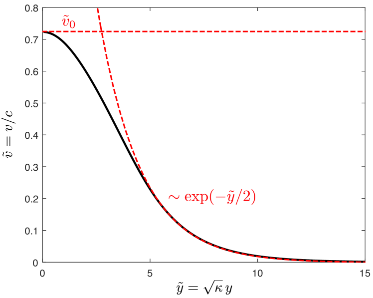
Figure 2: Optimum dimensionless soliton velocity, $\tilde{v}=v/c$, as a function of dimensionless domain wall separation $\tilde{y}$, obtained by minimizing $V_{\parallel}(\tilde{y})$ with respect to $\tilde{v}$.

The effective potential still depends on the dimensionless velocity $\tilde{v}$. This parameter can be expressed as a function of the domain-wall separation $\tilde{y}$ if we minimize the energy of the isolated chain, $E_{\parallel}=V_{\parallel}(\tilde{y})$, with respect to $\tilde{v}$. The resulting function $\tilde{v}(\tilde{y})$ is determined numerically and plotted in Fig. 2. While for $\tilde{y}\to 0$ the velocity approaches a constant $\tilde{v}_{0}\approx 0.725$, for large domain-wall separations the velocity decays exponentially, $\tilde{v}\simeq 2.85\exp(-|\tilde{y}|/2)$.

Let us first investigate the asymptotic behavior of the contributions $V_{\parallel}$ (13) and $V_{\perp}$ (14) to the potential. At large distances ($|\tilde{y}|\to\infty$), the intra-chain contribution $V_{\parallel}(\tilde{y})$ approaches the energy $2E_{0}$ of two free solitons at rest, while the inter-chain contribution grows linearly,

$$\frac{V_{\perp}(\tilde{y})}{E_{0}}\approx\frac{g_{\perp}}{\kappa}|\tilde{y}|.$$ (16)

This is the same behavior as for point-like domain walls. This is expected since at large distances the spatial extent $\xi$ of the solitons becomes irrelevant. Expressed in terms of the microscopic parameters, using Eqs. (3), (12) and the definition of $E_{0}$ (15), we can express the asymptotic result in terms of the microscopic parameters to recover $V\sim n_{\perp}J_{\perp}|y|/a$.

At small separations ($\tilde{y}\ll 1$), both contributions are quadratic,

$$\frac{V_{\parallel}(\tilde{y})}{E_{0}} \approx \frac{4-3\tilde{v}_{0}^{2}}{6\tilde{v}_{0}^{2}\sqrt{1-\tilde{v}_{0}^{2}}^{3}}\tilde{y}^{2}\approx 2.35\,\tilde{y}^{2},$$ (17)

$$\frac{V_{\perp}(\tilde{y})}{E_{0}} \approx \frac{1}{4\tilde{v}_{0}^{2}\sqrt{1-\tilde{v}_{0}^{2}}}\frac{g_{\perp}}{\kappa}\tilde{y}^{2}\approx 0.69\frac{g_{\perp}}{\kappa}\tilde{y}^{2},$$ (18)

which is the result of the gradual annihilation of the extended soliton and anti-soliton.

The intra-chain contribution $V_{\parallel}(\tilde{y})$ and the full confinement potential $V(\tilde{y})=V_{\parallel}(\tilde{y})+V_{\perp}(\tilde{y})$ are shown in Fig. 3 as a function of the dimensionless domain-wall separation $\tilde{y}=\sqrt{\kappa}y$. They display the asymptotic behavior discussed above. The crossover from linear to quadratic behavior of $V(\tilde{y})$ occurs at $\tilde{y}=1$. Since the crossover is expected to occur when the solitons start to overlap (see Fig. 1b), we can identify the size of the solitons as

$$\xi\simeq\frac{1}{\sqrt{\kappa}}=a\sqrt{\frac{J}{2\alpha}}.$$ (19)

This equation shows that the size of the solitons is controlled by the relative strength of the Ising anisotropy, $\alpha/J$. In the case of strong Ising anisotropy, the size of the solitons is of the order of the lattice spacing $a$. On the other hand, in systems with very weak anisotropy, the spatial extent of soliton domain walls can be of the order of hundreds of lattice spacings.

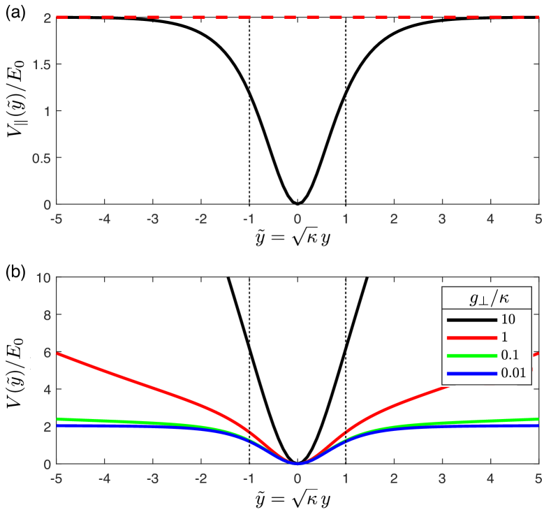
Figure 3: (a) In-chain $\textup{K}\overline{\textup{K}}$ potential $V_{\parallel}(\tilde{y})$ as a function of dimensionless separation $\tilde{y}=\sqrt{\kappa}y$. At large separations, $V_{\parallel}$ approaches the energy $2E_{0}$ of two free solitons. Due to the gradual destructive interference of the solitons, $V_{\parallel}$ is rendered quadratic at small distances. The crossover occurs at $\tilde{y}=1$, corresponding to a soliton size $\xi=1/\sqrt{\kappa}$. (b) The same crossover is found in the effective confinement potential $V(\tilde{y})=V_{\parallel}(\tilde{y})+V_{\perp}(\tilde{y})$. At large separations the potential is linear, $V(\tilde{y})/E_{0}\approx(g_{\perp}/\kappa)|\tilde{y}|$, while at small separations the potential is quadratic due to the gradual annihilation of the extended solitons.

III.2 Bound-State Spectrum

The gradual destructive interference of extended solitons at separations $y<\xi$ weakens the confinement potential and renders it quadratic. In the following we will consider the solitons as point-like particles interacting with the effective non-linear potential $V(y)$ and determine the discrete bound-state spectrum from the solution of the one-dimensional Schrödinger equation

$$-\frac{\hbar^{2}}{2\mu}\frac{\mathrm{d}^{2}\psi}{\mathrm{d}y^{2}}+V(y)\psi=\epsilon\psi$$ (20)

for the effective one-body problem for the relative coordinate $y$ of the soliton pair. Here $\mu=m/2$ denotes the reduced mass in terms of the single-soliton mass $m$.

As a point of reference, let us first consider the limit of very strong Ising anisotropy. In this case the potential is linear down to lattice scale, $V(y)=\lambda|y|$, and the theory of linear confinementGrenier et al. (2015); Wang et al. (2015); Bera et al. (2017); Gannon et al. (2019); Coldea et al. (2010) applies. The resulting bound-state energies are given byWang et al. (2015)

$$\epsilon_{j}^{>}=2E_{0}+\xi_{j}\lambda^{2/3}\left(\frac{\hbar^{2}}{\mu}\right)^{1/3},$$ (21)

where $\xi_{j}$ are the negative zeroes of the Airy function, $\textrm{Ai}(-\xi_{j})=0$, $\xi_{1}\approx 2.338$, $\xi_{2}\approx 4.088$, $\xi_{3}\approx 5.520$, $\ldots$.

In the limit of very weak anisotropy on the other hand, the confinement potential is quadratic over a significant range, $V(y)\simeq\frac{1}{2}\mu\omega^{2}y^{2}$, giving rise to equidistant energy levels

$$\epsilon_{j}^{<}=\hbar\omega\left(j+\frac{1}{2}\right).$$ (22)

Due to the crossover of $V(y)$ from quadratic behavior at short distances to linear behavior at large distances, we expect to a related crossover in the energy level spacing of the bound states. The strongly bound states at low energies will be almost equidistant, as described by $\epsilon_{j}^{<}$ (22), while the weakly bound states at higher energies will approach the sequence $\epsilon_{j}^{>}$ (21). This crossover is controlled by the strength of the Ising anisotropy $\alpha/J$.

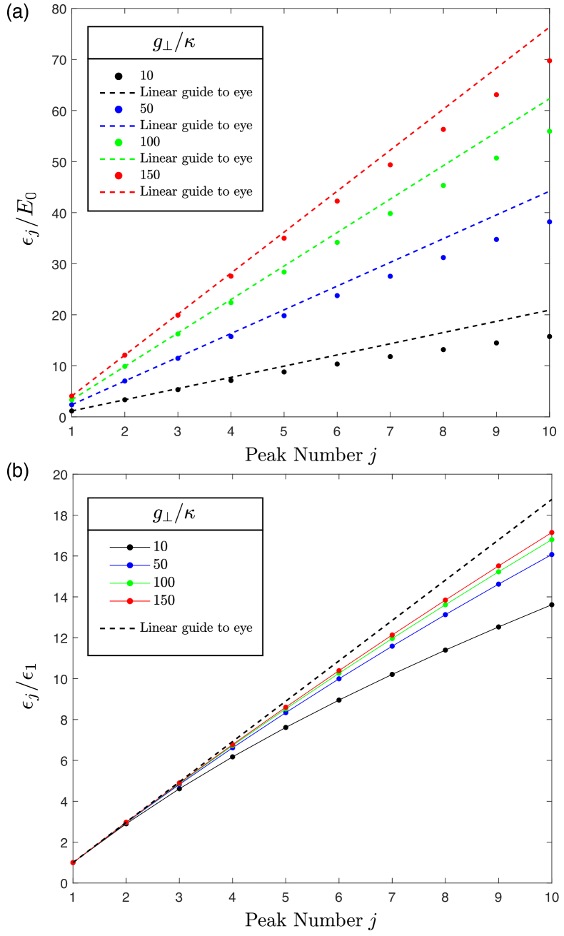
Figure 4: (a) Soliton-antisoliton bound-state energies $\epsilon_{j}$ in units of the single soliton energy $E_{0}$ for different ratios $g_{\perp}/\kappa$ and $S=5/2$. The corresponding confinement potentials are shown in the inset. (b) Same spectra but normalized by the energy $\epsilon_{1}$ of the first bound state. For larger values of $g_{\perp}/\kappa$ the level spacing becomes more harmonic oscillator like (dashed line).

In order to obtain the bound-state spectrum for the full confinement potential we transform the Schrödinger equation (20) to dimensionless units,

$$-\frac{1}{2S^{2}}\frac{\mathrm{d}^{2}\psi}{\mathrm{d}\tilde{y}^{2}}+\tilde{V}(\tilde{y})\psi=\tilde{\epsilon}\psi,$$ (23)

$\tilde{y}=\sqrt{\kappa}y$, $\tilde{\epsilon}=\epsilon/E_{0}$ and $\tilde{V}(\tilde{y})=V_{\parallel}(\tilde{y})/E_{0}+V_{\perp}(\tilde{y})/E_{0}$ (13,14), and then numerically solve the equation, using the finite-element method implemented in Mathematica.Mat

In Fig. 4(a) the resulting bound-state energies $\epsilon_{j}/E_{0}$ for $S=5/2$ (value for CaFe₂O₄) and different values of $g_{\perp}/\kappa$ are shown. In the regime of large $g_{\perp}/\kappa$, the dominant contribution to the confinement potential comes from the frustrated inter-chain coupling. The tightly bound states have almost equidistant energy levels with spacing $\Delta\epsilon/E_{0}\approx(1.17/S)\sqrt{g_{\perp}/\kappa}$, as expected for the asymptotic quadratic form of the potential at small distances, $\tilde{V}(\tilde{y})\approx\tilde{V}_{\perp}(\tilde{y})\approx 0.69(g_{\perp}/\kappa)\tilde{y}^{2}$. At higher energies, the level spacing is reduced because of the crossover of the potential to a linear form at large distances. Normalizing the energies by the energy $\epsilon_{1}$ of the first bound state (see Fig. 4(b)), it is apparent that the spectrum becomes more like that of a harmonic oscillator if the value of $g_{\perp}/\kappa$ is increased.

IV Application to Calcium Ferrite

In this section we will apply our theory of non-linear soliton confinement to the $S=5/2$ antiferromagnet CaFe₂O₄. Recent neutron scattering experimentsStock et al. (2016) found signatures of solitary magnons in this material with a sequence of nine quantized excitations below the magnetic ordering transition at $T_{\textrm{N}}\approx 200$ K.

CaFe₂O₄ has a complex magnetic phase diagram due a competition between two different spin arrangements, termed the $A$ and $B$ phases.Corliss et al. (1967) The magnetic structure of the $B$ phase, which dominates at high temperatures, consists of antiferromagnetic zig-zag chains along the $b$ axis (see Fig. 5). The moments are oriented along $b$ due to a small easy-axis anisotropy.

The $A$ phase might coexist with the $B$ phase over the full temperature range but becomes clearly visible only below 170 K, which has been identified as its onset temperature in early studies.Corliss et al. (1967) The two phases are distinguished by their $c$-axis stacking of ferromagnetic $b$-axis stripes: the $B$ phase consists of stripes with antiferromagnetic alignment within the zig-zag chain, $(\uparrow\downarrow)(\uparrow\downarrow)$, while in the $A$ phase the zig-zag chains are ferromagnetic with stacking $(\uparrow\uparrow)(\downarrow\downarrow)$ along $c$.Corliss et al. (1967) It has been suggestedStock et al. (2016) that the gradual increase of the $A$ phase component is linked to anti-phase domain boundaries along $c$, combined with a continuous change of the Fe-O-Fe bond angle which controls the strength and sign of the super-exchangeMizuno et al. (1998); Shimizu et al. (2003) between the two legs forming the zig-zag chain. This scenario is supported by the presence of diffuse scattering rods along the $L$ direction and spin-wave excitations that show magnetic order in the $ab$-plane with short-ranged correlations along $c$.Stock et al. (2016)

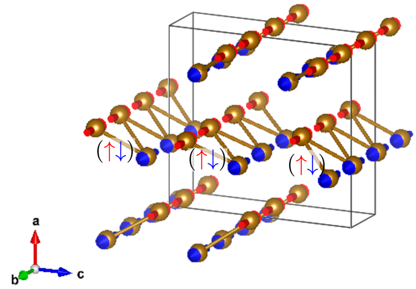
Figure 5: Magnetic structure in the high-temperature B phase of CaFe₂O₄,Stock et al. (2016) showing antiferromagnetic zig-zag chains along the $b$ axis. The system exhibits a weak easy-axis anisotropy along $b$. Calcium Ferrite is based upon an orthorhombic unit cell (space group 62 $Pnma$) with dimensions $a=9.230$ Å, $b=3.017$ Å, and $c=10.689$ Å.Hill et al. (1956); Decker and Kasper (1957)

From now on we focus on the $B$ phase that completely dominates at high temperatures where the discrete excitations are observed. As pointed out in Ref. [Stock et al., 2016], the level spacing of the excitations cannot be explained based on the linear confinement picture. This led the authors to speculate that the discrete nature of the excitations is not due to interaction-driven bound-state formation but instead a result of spatial confinement along the $c$ axis. Here we show that an effective non-linear interaction potential arising from the extended nature of solitons in CaFe₂O₄ would lead to a bound-state spectrum that is consistent with the data.

Let us first inspect the discrete energy-level spectrum presented in Ref. [Stock et al., 2016] more closely. The excitations can only be observed above the spin wave anisotropy gap, which shows a strong temperature dependence. The gap opens below $T_{\textrm{N}}\approx 200$ K and saturates to a value of $\Delta\approx 3$ meV below 100 K. For this reason, the lowest energy excitation can only be resolved slightly below $T_{\textrm{N}}$ where strong fluctuations almost completely fill in the gap. The data at 200 K show six discrete energy levels below 2 meV. At 150 K the spin-wave gap almost completely masks this energy range. Instead three energy levels become visible above around 1.8 meV. In Ref. [Stock et al., 2016] it was assumed that the discrete excitations energies have a negligible temperature dependence and that the three levels observed at 150 K are the continuation of the energy sequence at 200 K.

If the discrete excitations were due to soliton bound-state formation one would expect the excitation spectrum to depend upon temperature. Based on our theory, we expect that the main temperature dependence enters through the effective mean-field coupling $g_{\perp}$ to neighboring chains. Since $g_{\perp}$ is proportional to the magnetization of the system, it increases as temperature is lowered. This would explain why the bound states at 150 K have a larger level spacing than those at 200 K.

Moreover, magnetoelastic effects and small changes to the Fe-O-Fe bond angle close to the threshold at which the superexchange would change sign could give rise to a non-negligible temperature dependence of magnetic exchange couplings.Songvilay et al. (2020) Finally, the gradual onset of the $A$ phase could give rise to additional effects which might obscure the soliton signal in the neutron scattering experiment

IV.1 Experimental Results

Here we present previously unpublished data that were collected alongside those published in Ref. [Stock et al., 2016]. Instead of combining measurements at different temperatures we focus on $T=200$ K, allowing us to trace the excitations down to very low energies.

Our experiments were performed on single crystals of CaFe₂O₄ grown using a mirror furnace. High momentum and energy resolution data was obtained using the OSIRIS backscattering spectrometer located at the ISIS Neutron and Muon Source.Andersen et al. (2002) A white beam of neutrons is incident on the sample and the final energy of the scattered neutrons is fixed at $E_{f}=1.84$ meV using cooled graphite analyzers. A cooled Beryllium filter was used on the scattered side to reduce background. The default configuration is set for a symmetric dynamic range of $\pm 0.5$ meV, however by shifting the incoming energy band width using a chopper the dynamic range was extended into the inelastic region. For this experimental setup, the elastic energy resolution (full-width) was $2\delta E=0.025$ meV. Due to kinematic constraints, we focussed our measurements around $\mathbf{Q}=(2,0,0)$ (r.l.u) so that the quantized excitations could be tracked up to energy transfers of $\sim 3$ meV.

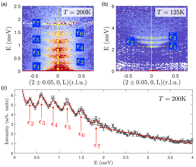
Figure 6: (a) High resolution low energy data recorded on OSIRIS at $T=200$ K, showing seven clearly discernible excitations $\epsilon_{j}$ at $\mathbf{Q}=(2,0,0)$ (r.l.u.). The modes show a weak quadratic dispersion along $L$, highlighted by dashed yellow lines. (b) At $T=125$ K the spin-wave gap masks excitations below 2 meV. Above this energy, three additional excitations $\tilde{\epsilon}_{j}$ are visible. (c) Scattering intensity at $\mathbf{Q}=(2,0,0)$ as a function of energy. Peaks at $\epsilon_{2},\ldots,\epsilon_{7}$ are clearly resolved. The energy $\epsilon_{1}$ is below the elastic line.

As shown in Fig. 6(a), at 200 K we find seven discrete excitations in low energy scattering data below 2 meV, located at $\mathbf{Q}=(2,0,0)$ and with a weak quadratic dispersion along $L$. The intensities are integrated over a small window of $2\pm 0.05$ r.l.u. in the $H$ direction. The excitations have an almost linear level spacing $\Delta\epsilon\approx 0.3$ meV, in very good agreement with previous results.Stock et al. (2016)

In comparison, at 125 K the spin-wave gap masks the excitations below 2 meV but three discrete excitations at $\tilde{\epsilon}_{1}$, $\tilde{\epsilon}_{2}$ and $\tilde{\epsilon}_{3}$ are visible above this energy (Fig. 6(b)). The modes are at slightly higher energies than those identified at 150 K in Ref. [Stock et al., 2016], suggesting that there might exists a non negligible temperature dependence. In the following we will discard the excitations above 2 meV since they cannot be resolved at 200 K.

In Fig. 6(c), the scattering intensity at 200 K as a function of energy at $\mathbf{Q}=(2,0,0)$ is shown. Peaks at the energy levels $\epsilon_{2},\ldots\epsilon_{7}$ are very clearly visible. The first excitation $\epsilon_{1}$ is beneath the incoherent background in the OSIRIS data and cannot be resolved in the energy cut. However, the energy $\epsilon_{1}$ can be estimated thanks to the weak quadratic dispersion along $L$ (see dashed yellow lines in Fig. 6(a)).

IV.2 Fitting to Non-Linear Confinement Model

We now investigate whether the seven discrete excitations measured at 200 K can be explained in terms of soliton bound-state formation. The quantized excitations $\epsilon_{j}$ extracted from the neutron scattering experiment are shown as open circles in Fig. 7. For the levels $j=2,\ldots,7$ we estimate the experimental error $\delta\epsilon_{j}$ from the full peak width at half maximum. For the lowest energy state, which is masked by the incoherent background of the elastic line, we assume a larger uncertainty of $\delta\epsilon_{1}\approx 0.15$ meV.

As point of reference, we first assume a linear confinement potential. In this case the soliton bound-state energies would be given by $\epsilon_{j}=A+B\xi_{j}$, where $\xi_{j}$ are the negative zeroes of the Airy function and the energies $A$ and $B$ are related to the soliton rest mass and the slope of the linear potential, as defined in Eq. (21). Here we use $A$ and $B$ as free fitting parameters, not imposing any additional constraints. The resulting best case scenario for the linear-confinement model (dashed magenta line in Fig. 7) strongly deviates from the data, showing that the discrete excitations in CaFe₂O₄ cannot be understood in terms of a linear confinement of solitons.

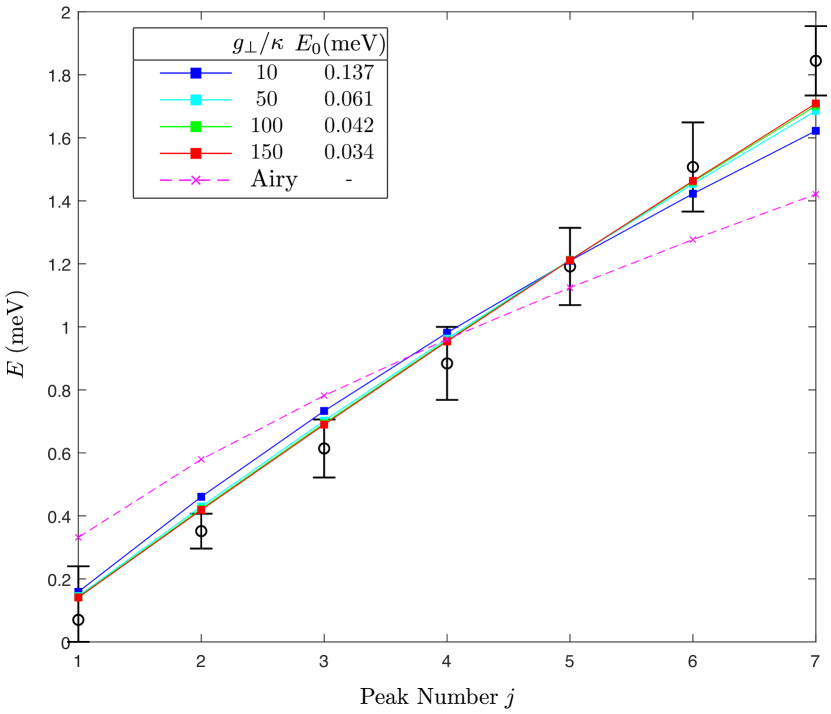
Figure 7: Comparison between the measured excitation energies (open circles) and the soliton bound state energies calculated from the non-linear confinement model. The figure shows best fits to the data for different values of $g_{\perp}/\kappa$. The quality of the fits improves with increasing values of $g_{\perp}/\kappa$ and decreasing soliton energy $E_{0}$. Good agreement is achieved for $g_{\perp}/\kappa\geq 50$. For comparison, the best fit of the linear-confinement model is shown in magenta.

The bound-state spectra obtained from the effective non-linear confinement potential depend on two parameters, the soliton rest energy $E_{0}=2\rho_{S}\sqrt{\kappa}$ and the dimensionless ratio $g_{\perp}/\kappa$. For a given value of $g_{\perp}/\kappa$ we obtain the best fit to the data $\{\epsilon_{j}\pm\delta\epsilon_{j}\}$ by minimizing

$$\chi^{2}=\sum_{j}\left(\frac{\epsilon_{j}^{\textrm{th}}(E_{0})-\epsilon_{j}}{\delta\epsilon_{j}}\right)^{2}$$ (24)

with respect to $E_{0}$, where $\{\epsilon_{j}^{\textrm{th}}\}$ refers to the spectrum obtained from our theoretical model.

As shown in Fig. 7, the fits improve with increasing values of $g_{\perp}/\kappa$, corresponding to decreasing optimum values of $E_{0}$. A good description of our data is obtained for $g_{\perp}/\kappa=50$ and $E_{0}=0.061$ meV. Although for larger values of $g_{\perp}/\kappa$ the fits continue to improve slightly, the soliton size $\xi=1/\sqrt{\kappa}=2\rho_{S}/E_{0}$ would eventually become too large for our theoretical description to be valid.

For $g_{\perp}/\kappa=50$ the levels are almost equidistant, showing that the first 7 levels fall in the harmonic potential regime. To check consistency, we calculate the average mean-square displacement of the soliton bound states, $d_{j}=\sqrt{\langle\hat{y}^{2}\rangle_{j}}$, using the approximate quadratic potential (17) at small distances, $y<\xi$. For the highest level resolved experimentally we obtain $d_{7}/\xi\approx 0.55<1$, indicating a significant overlap of the bound solitons.

The parameters $\rho_{S}$, $g_{\perp}$ and $\kappa$ describe the long-wavelength, low energy behavior of the system. This effective continuum description is completely generic and applies to any system of weakly coupled antiferromagnetic spin chains in the the large-$S$ limit.

For illustrative purposes, we have considered a minimal spin model (1) and established how the effective parameters in the continuum field theory depend on the exchange couplings and single-ion anisotropy of the lattice Hamiltonian (see Eqs. (3),(12)). However, this model is too simplistic for CaFe₂O₄, e.g. it neglects the ferromagnetic exchange along the legs of the zig-zag chains, which is likely to be rather strong. Unfortunately, spin-wave excitations, which could be used to determine a more realistic spin model, have not been measured in the $B$ phase, but only at 4 K where the competing $A$ phase dominates.Stock et al. (2016)

On the other hand, close to the Néel transition collective fluctuations are very strong, leading to universal behavior detached from microscopic details. The spin stiffness is expected to vanish continuously at $T_{\textrm{N}}$, satisfying Josephson scaling $\rho_{S}\sim(T_{\textrm{N}}-T)^{(d-2)\nu}$ [Goldenfeld, 2019,Chubukov et al., 1994], where $\nu$ is the correlation-length exponent and $d$ the spatial dimension. The bound states are observed slightly below $T_{\textrm{N}}$ where the stiffness is strongly reduced. If we assume $\rho_{S}/a\approx 3$ meV, which is of the order of the gap and about a tenth of the spin-wave bandwidth at low temperature, we would obtain a soliton size of about 100 lattice constants, $\xi/a=2(\rho_{S}/a)/E_{0}\approx 100$.

As suggested in Ref. [Stock et al., 2016], quantized excitations in CaFe₂O₄ could also arise from anti-phase boundaries along the $c$ axis that separate the two competing magnetic phases and lead to spatial confinement. This mechanism is unlikely to be relevant close to $T_{\textrm{N}}$ where the phase boundaries are dynamic and the $A$ phase is almost completely absent. At low temperatures, however, the anti-phase domain boundaries become static and carry an uncompensated moment that can be tuned by a magnetic field.Stock et al. (2017) The presence of uncompensated spins at phase or domain boundaries is also confirmed by thin-film experiments.Damerio et al. (2020) Isolated clusters of such orphan spins would provide a natural explanation of the discrete magnetic excitations observed at very low temperatures below the spin-wave gap.Stock et al. (2017)

V Discussion

To summarize, we have developed a theory for the confinement of solitons in weakly coupled, large-spin antiferromagnetic chains with easy-axis anisotropy. Below the Néel transition the frustrated interchain coupling generates an attractive potential that leads to the formation of soliton-antisoliton bound states. This mechanism is analogous to the confinement of spinons in $S=1/2$ antiferromagnetic XXZ chainsGrenier et al. (2015); Wang et al. (2015); Bera et al. (2017); Gannon et al. (2019) or of domain-wall kinks in ferromagnetic Ising chains.Coldea et al. (2010) But while for these systems the domain-wall defects can be considered as point like, leading to a linear confinement potential, semi-classical solitons have a significant spatial extent. This renders the effective confinement potential quadratic on length scales smaller than the size of the solitons, giving rise to a crossover in the energy level spacing of the bound states.

The $S=5/2$ antiferromagnet CaFe₂O₄ is a good candidate system to test our theory since this material shows a sequence of discrete low-energy excitationsStock et al. (2016) below $T_{\textrm{N}}$ and exhibits a magnetic structure that consists of antiferromagnetic zig-zag chains, subject to a weak Ising anisotropy.Corliss et al. (1967) Our inelastic neutron scattering experiments, performed slightly below $T_{\textrm{N}}$, confirmed the existence of seven discrete excitations below 2 meV with an almost linear level spacing. Our analysis shows that the quantized excitations can be explained well by the non-linear confinement of large, spatially extended solitons. We argue that strong collective fluctuations close to $T_{\textrm{N}}$ play a crucial role, collapsing the anisotropy gap and strongly reducing the spin stiffness.

There are many possible ways in which our theory can be extended to describe a rich variety of physical systems. To model materials with strong interchain coupling one can include the feedback of the effective field from neighboring chains on the soliton dynamics. Such a staggered field changes the equation of motion to a double sine-Gordon equation which is no longer integrable but nonetheless can be solved numerically.Campbell et al. (1986); Gani and Kudryavtsev (1999) Staggered fields could also be generated by applying external fields in systems with staggered $g$ tensors.Oshikawa and Affleck (1997); Affleck and Oshikawa (1999) Since solitons and antisolitons have opposite chirality it would be interesting to study the effects of a weak Dzyaloshinskii-Moriya interaction which would introduce chirality in the antiferromagnetic background. Finally, one might include finite-lifetime effects due to collisions of bound soliton pairs and the interactions with spin-wave excitations.

Thanks to recent advances in crystal growth and neutron scattering technology it is now possible to resolve soliton bound states at very low energies. The relevant theoretical parameters in the effective long-wavelength description, such as the spin stiffness, spin-wave velocity and staggered magnetization, vanish at the continuous Néel transition, showing characteristic power-law behavior. The measurement of soliton bound states close to the transition could therefore provide a novel route to study universal critical behavior in inelastic neutron scattering experiments.

Acknowledgements The authors thank E. Christou, A. Green, A. James and M. Songvilay for useful discussions. F.K. acknowledges financial support from EPSRC under Grant No. EP/P013449/1. S.W.C was supported by the DOE under Grant No. DOE: DE-FG02-07ER46382. C.S. and H.L. wish to thank the EPSRC and the STFC for funding. H.L. was co-funded by the ISIS facility development studentship programme. Experiments at the ISIS Neutron and Muon Source were supported by a beamtime allocation RB1510445 (DOI: 10.5286/ISIS.E.RB1510445) from the Science and Technology Facilities Council.

References

- Collins and Perry (1975) J. C. Collins and M. J. Perry, Phys. Rev. Lett. 34, 1353 (1975).
- Berezinsky (1971) V. Berezinsky, Sov. Phys. JETP 32, 493 (1971).
- Kosterlitz and Thouless (1973) J. M. Kosterlitz and D. J. Thouless, Journal of Physics C: Solid State Physics 6, 1181 (1973).
- Tomonaga (1950) S. Tomonaga, Progress of Theoretical Physics 5, 544 (1950).
- Luttinger (1963) J. M. Luttinger, Journal of Mathematical Physics 4, 1154 (1963).
- Haldane (1981) F. D. M. Haldane, Journal of Physics C: Solid State Physics 14, 2585 (1981).
- Faddeev and Takhtajan (1981) L. Faddeev and L. Takhtajan, Physics Letters A 85, 375 (1981).
- Bougourzi et al. (1996) A. H. Bougourzi, M. Couture, and M. Kacir, Phys. Rev. B 54, R12669 (1996).
- Karbach et al. (1997) M. Karbach, G. Müller, A. H. Bougourzi, A. Fledderjohann, and K.-H. Mütter, Phys. Rev. B 55, 12510 (1997).
- Caux et al. (2008) J.-S. Caux, J. Mossel, and I. P. Castillo, Journal of Statistical Mechanics: Theory and Experiment 2008, P08006 (2008).
- Bethe (1931) H. Bethe, Zeitschrift für Physik 71, 205 (1931).
- Mourigal et al. (2013) M. Mourigal, M. Enderle, A. Klöpperpieper, J.-S. Caux, A. Stunault, and H. M. Rønnow, Nature Physics 9, 435 (2013).
- Bera et al. (2017) A. K. Bera, B. Lake, F. H. L. Essler, L. Vanderstraeten, C. Hubig, U. Schollwöck, A. T. M. N. Islam, A. Schneidewind, and D. L. Quintero-Castro, Phys. Rev. B 96, 054423 (2017).
- Gannon et al. (2019) W. J. Gannon, I. A. Zaliznyak, L. S. Wu, A. E. Feiguin, A. M. Tsvelik, F. Demmel, Y. Qiu, J. R. D. Copley, M. S. Kim, and M. C. Aronson, Nature Communications 10, 1123 (2019).
- Wu et al. (2019) L. S. Wu, S. E. Nikitin, Z. Wang, W. Zhu, C. D. Batista, A. M. Tsvelik, A. M. Samarakoon, D. A. Tennant, M. Brando, L. Vasylechko, M. Frontzek, A. T. Savici, G. Sala, G. Ehlers, A. D. Christianson, M. D. Lumsden, and A. Podlesnyak, Nature Communications 10, 698 (2019).
- Oshikawa and Affleck (1997) M. Oshikawa and I. Affleck, Phys. Rev. Lett. 79, 2883 (1997).
- Affleck and Oshikawa (1999) I. Affleck and M. Oshikawa, Phys. Rev. B 60, 1038 (1999).
- Dender et al. (1996) D. C. Dender, D. Davidović, D. H. Reich, C. Broholm, K. Lefmann, and G. Aeppli, Phys. Rev. B 53, 2583 (1996).
- Dender et al. (1997) D. C. Dender, P. R. Hammar, D. H. Reich, C. Broholm, and G. Aeppli, Phys. Rev. Lett. 79, 1750 (1997).
- Pytte (1974) E. Pytte, Phys. Rev. B 10, 4637 (1974).
- Ishimura and Shiba (1977) N. Ishimura and H. Shiba, Progress of Theoretical Physics 57, 1862 (1977).
- Müller et al. (1981) G. Müller, H. Thomas, H. Beck, and J. C. Bonner, Phys. Rev. B 24, 1429 (1981).
- Essler et al. (2003) F. H. L. Essler, A. Furusaki, and T. Hikihara, Phys. Rev. B 68, 064410 (2003).
- Lake (2005) B. Lake, Nature Physics 1, 143 (2005).
- Braun et al. (2005) H.-B. Braun, J. Kulda, B. Roessli, D. Visser, K. W. Krämer, H.-U. Güdel, and P. Böni, Nature Physics 1, 159 (2005).
- Kenzelmann et al. (2004) M. Kenzelmann, Y. Chen, C. Broholm, D. H. Reich, and Y. Qiu, Phys. Rev. Lett. 93, 017204 (2004).
- Umegaki et al. (2015) I. Umegaki, H. Tanaka, N. Kurita, T. Ono, M. Laver, C. Niedermayer, C. Rüegg, S. Ohira-Kawamura, K. Nakajima, and K. Kakurai, Phys. Rev. B 92, 174412 (2015).
- Zvyagin et al. (2004) S. A. Zvyagin, A. K. Kolezhuk, J. Krzystek, and R. Feyerherm, Phys. Rev. Lett. 93, 027201 (2004).
- Liu et al. (2019) J. Liu, S. Kittaka, R. D. Johnson, T. Lancaster, J. Singleton, T. Sakakibara, Y. Kohama, J. van Tol, A. Ardavan, B. H. Williams, S. J. Blundell, Z. E. Manson, J. L. Manson, and P. A. Goddard, Phys. Rev. Lett. 122, 057207 (2019).
- Grenier et al. (2015) B. Grenier, S. Petit, V. Simonet, E. Canévet, L.-P. Regnault, S. Raymond, B. Canals, C. Berthier, and P. Lejay, Phys. Rev. Lett. 114, 017201 (2015).
- Wang et al. (2015) Z. Wang, M. Schmidt, A. K. Bera, A. T. M. N. Islam, B. Lake, A. Loidl, and J. Deisenhofer, Phys. Rev. B 91, 140404 (2015).
- Coldea et al. (2010) R. Coldea, D. A. Tennant, E. M. Wheeler, E. Wawrzynska, D. Prabhakaran, M. Telling, K. Habicht, P. Smeibidl, and K. Kiefer, Science 327, 177 (2010).
- Stock et al. (2016) C. Stock, E. E. Rodriguez, N. Lee, M. A. Green, F. Demmel, R. A. Ewings, P. Fouquet, M. Laver, C. Niedermayer, Y. Su, K. Nemkovski, J. A. Rodriguez-Rivera, and S.-W. Cheong, Phys. Rev. Lett. 117, 017201 (2016).
- Haldane (1983) F. D. M. Haldane, Phys. Rev. Lett. 50, 1153 (1983).
- Yosida (2010) K. Yosida, Theory of Magnetism, Series: Springer Series in Solid-State Sciences, Vol. 122 (Springer, Berlin Heidelberg, 2010).
- Sachdev (2011) S. Sachdev, Quantum Phase Transitions, 2nd ed. (Cambridge University Press, 2011).
- Fradkin (2013) E. Fradkin, Field Theories of Condensed Matter Physics, 2nd ed. (Cambridge University Press, 2013).
- Perring and Skyrme (1962) J. Perring and T. Skyrme, Nuclear Physics 31, 550 (1962).
- Scharf et al. (1992) R. Scharf, Y. S. Kivshar, A. Sánchez, and A. R. Bishop, Phys. Rev. A 45, R5369 (1992).
- Crampin and Saunders (1986) M. Crampin and D. Saunders, Reports on Mathematical Physics 23, 327 (1986).
- Rogers and Schief (2002) C. Rogers and W. K. Schief, Bäcklund and Darboux Transformations: Geometry and Modern Applications in Soliton Theory, Cambridge Texts in Applied Mathematics (Cambridge University Press, 2002).
- Cuenda et al. (2011) S. Cuenda, N. Quintero, and A. Sanchez, Discrete and Continuous Dynamical Systems. Series S 5 (2011).
- Campbell et al. (1986) D. K. Campbell, M. Peyrard, and P. Sodano, Physica D: Nonlinear Phenomena 19, 165 (1986).
- Gani and Kudryavtsev (1999) V. A. Gani and A. E. Kudryavtsev, Phys. Rev. E 60, 3305 (1999).
- (45) Wolfram Research, Inc., Mathematica, Version 12.1, Champaign, IL (2020).
- Corliss et al. (1967) L. M. Corliss, J. M. Hastings, and W. Kunnmann, Phys. Rev. 160, 408 (1967).
- Mizuno et al. (1998) Y. Mizuno, T. Tohyama, S. Maekawa, T. Osafune, N. Motoyama, H. Eisaki, and S. Uchida, Phys. Rev. B 57, 5326 (1998).
- Shimizu et al. (2003) T. Shimizu, T. Matsumoto, A. Goto, T. V. Chandrasekhar Rao, K. Yoshimura, and K. Kosuge, Phys. Rev. B 68, 224433 (2003).
- Hill et al. (1956) P. M. Hill, H. S. Peiser, and J. R. Rait, Acta Crystallographica 9, 981 (1956).
- Decker and Kasper (1957) B. F. Decker and J. S. Kasper, Acta Crystallographica 10, 332 (1957).
- Songvilay et al. (2020) M. Songvilay, S. Petit, M. Koza, S. Rols, E. Suard, V. Skumryev, C. Martin, and F. Damay, Phys. Rev. B 101, 014407 (2020).
- Andersen et al. (2002) K. Andersen, D. Martín y Marero, and M. Barlow, Applied Physics A 74, s237 (2002).
- Goldenfeld (2019) N. Goldenfeld, Lectures on Phase Transitions and the Renormalization Group (CRC Press, Taylor & Francis Group, Boca Raton, 2019).
- Chubukov et al. (1994) A. V. Chubukov, S. Sachdev, and J. Ye, Phys. Rev. B 49, 11919 (1994).
- Stock et al. (2017) C. Stock, E. E. Rodriguez, N. Lee, F. Demmel, P. Fouquet, M. Laver, C. Niedermayer, Y. Su, K. Nemkovski, M. A. Green, J. A. Rodriguez-Rivera, J. W. Kim, L. Zhang, and S.-W. Cheong, Phys. Rev. Lett. 119, 257204 (2017).
- Damerio et al. (2020) S. Damerio, P. Nukala, J. Juraszek, P. Reith, H. Hilgenkamp, and B. Noheda, (2020), arXiv:2001.11446 .