Suppression of superconducting parameters by correlated quasi-two-dimensional magnetic fluctuations

Abstract

We consider a clean layered magnetic superconductor in which a continuous magnetic transition takes place inside a superconducting state. We assume that the exchange interaction between superconducting and magnetic subsystems is weak so that superconductivity is not destroyed at the magnetic transition. A representative example of such material is RbEuFe₄As₄. We investigate the suppression of the superconducting gap and superfluid density by correlated magnetic fluctuations in the vicinity of the magnetic transition. The influence of nonuniform exchange field on superconducting parameters is very sensitive to the relation between the magnetic correlation length, $\xi_{h}$, and superconducting coherence length $\xi_{s}$ defining the ’scattering’ ($\xi_{h}<\xi_{s}$) and ’smooth’ ($\xi_{h}>\xi_{s}$) regimes. As a small uniform exchange field does not affect the superconducting gap and superfluid density at zero temperature, smoothening of the spatial variations of the exchange field reduces its effects on these parameters. We develop a quantitative description of this ’scattering-to-smooth’ crossover for the case of quasi-two-dimensional magnetic fluctuations realized in RbEuFe₄As₄. Since the magnetic-scattering energy scale is comparable with the gap in the crossover region, the standard quasiclassical approximation is not applicable and full microscopic treatment is required. We find that the corrections to both the gap and superfluid density increase proportionally to $\xi_{h}$ until it remains much smaller than $\xi_{s}$. In the opposite limit, when the correlation length exceeds the coherence length both parameters have much weaker dependence on $\xi_{h}$. Moreover, the gap correction may decrease with increasing of $\xi_{h}$ in the immediate vicinity of the magnetic transition if it is located at temperature much lower than the superconducting transition. We also find that the crossover between the two regimes is unexpectedly broad: the standard scattering approximation becomes sufficient only when $\xi_{h}$ is substantially smaller than $\xi_{s}$.

I Introduction

Since the seminal work of Abrikosov and Gor’kov (AG)[1] and its extensions[2, 3, 4], the pair breaking by magnetic scattering has been established as a key concept in the physics of superconductivity. Its applications extend far beyond the original physical system for which the theory was developed, singlet superconductors with dilute magnetic impurities. In particular, the magnetic pair-breaking scattering strongly influences properties of superconducting materials containing an embedded periodic lattice of magnetic rare-earth ions. Several classes of such materials are known at present including magnetic Chevrel phases $\mathit{RE}$Mo₆X₈ ($\mathit{RE}$=rare-earth element and X=S, Se), ternary rhodium borides $\mathit{RE}$Rh₄B₄[5, 6, 7, 8], the rare-earth nickel borocarbides $\mathit{RE}$Ni₂B₂C[9, 10, 11], and recently discovered Eu-based iron pnictides[12, 13, 14, 15, 16]. Some of these compounds experience a magnetic-ordering transition inside the superconducting state. Depending on the strength of the exchange interaction between the rare-earth moments and conducting electrons, the magnetic transition may either destroy superconductivity or leave it intact. In any case, in the paramagnetic state, the fluctuating magnetic moments suppress superconductivity via magnetic scattering, similar to magnetic impurities. Near the ferromagnetic transition, the moments become strongly correlated which enhances the suppression. The AG theory has been generalized to describe this enhancement in several theoretical studies [17, 18]. A straightforward generalization, however, is only possible when the magnetic correlation length $\xi_{h}$ is shorter than the superconducting coherence length $\xi_{s}$ and this condition was always assumed in all theoretical works. For a continuous magnetic transition, there is always temperature range where this condition is violated, see Fig. 1(a). A small uniform exchange field does not modify superconducting gap in clean materials at zero temperature [19], because, in absence of free quasiparticles, the exchange field does not generate spin polarization of the Cooper-pair condensate. This observation indicates that, once the exchange field becomes smooth at the scale of coherence length, its efficiency in suppressing superconducting parameters at low temperatures diminishes. We can conclude that the existing treatments of the impact of correlated magnetic fluctuations on superconductivity are incomplete. A full theoretical description of this phenomenon requires consideration of the crossover between the ‘scattering’ and ‘smooth’ regimes illustrated in Fig. 1(a). For most magnetic superconductors, however, such full theory would be a mostly academic exercise, because the coherence length is typically much larger than the separation between magnetic ions. Consider, for example, the magnetic nickel borocarbide ErNi₂B₂C, which has the superconducting transition at T${}_{c}\approx$11 K and magnetic transition at T${}_{m}\approx$6 K [9, 10]. Its c-axis upper critical field has linear slope 0.3 T/K near T_c [20], from which we can estimate the in-plane coherence length at T_m as $\xi_{s}(T_{m})\approx$18 nm which is $\sim 54$ times larger than the distance between the Er³⁺ moments. Therefore, in this and similar materials the magnetic correlation length exceeds the coherence length only within an extremely narrow temperature range near the magnetic transition. The situation is very different, however, in Eu-based layered iron pnictides, such as RbEuFe₄As₄[13, 15, 16, 21]. The latter material has the superconducting transition at 36.5 K and the magnetic transition at 15K. The magnetism is quasi-two-dimensional: the Eu²⁺ moments have strong ferromagnetic interactions inside the magnetic layers with easy-plane anisotropy [22] and weak interactions between the magnetic planes leading to helical interlayer order[23, 24]. Due to the quasi-two-dimensional nature of magnetism, the in-plane magnetic correlation length smoothly grows within an extended temperature range. Another relevant material’s property is a very short in-plane coherence length, $\sim$1.5–2 nm, which is only 4–6 times larger than the distance between the magnetic ions. As a consequence, contrary to most magnetic superconductors, the magnetic correlation length exceeds the coherence length within a noticeable temperature range near the magnetic transition. Therefore, for the magnetic iron pnictides, the crossover between the ‘scattering’ and ‘smooth’ regimes is very relevant. Recent vortex imaging in RbEuFe₄As₄ with scanning Hall-probe spectroscopy revealed a significant increase of the London penetration depth in the vicinity of the magnetic transition[25]. This suggests that the exchange interaction between Eu²⁺ moments and Cooper pairs leads to substantial suppression of superconducting parameters near $T_{m}$.

The goal of this paper is to develop a quantitative theoretical description of the influence of correlated magnetic fluctuations on the superconducting gap and supercurrent response with a proper treatment of the crossover at $\xi_{h}\sim\xi_{s}$. The problem occurs to be technically challenging because in the crossover region the probability of magnetic scattering varies at the energy scale comparable with the temperature or the gap. This forbids the standard energy integration necessary for the quasiclassical approximation and requires a full microscopic consideration. In this consideration, one has to include the self-energy correction to the electronic spectrum and maintain the energy dependence of the scattering probability. As this accurate analysis is rather complicated, we utilize several simplifying assumptions. We limit ourselves to the case of weak exchange interaction and consider only the lowest-order corrections. We also assume the static approximation for magnetic fluctuations. This assumption is justified when typical frequency scale for magnetic fluctuations is smaller than the superconducting gap. Due to the critical slowing down, this always becomes valid sufficiently close to the transition. In the scattering regime, the dynamic effects have been investigated in several theoretical papers, see, e.g., [17, 26, 27]. The behavior is also sensitive to the dimensionality of magnetic fluctuations. Having in mind application to layered magnetic superconductors, such as RbEuFe₄As₄, we assume quasi-two-dimensional magnetic fluctuations. In this case the discussed effects are more pronounced than for three-dimensional magnetic fluctuations[18].

The paper is organized as follows. In Sec. II, we introduce the model for layered magnetic superconductors. In Sec. III, we evaluate the self energy caused by scattering by correlated magnetic fluctuations for arbitrary relation between the magnetic correlation length and coherence length and develop a quantitative description of the crossover between the scattering and smooth regimes. In Sec. IV, we use these results to evaluate the exchange correction to the gap. In Sec. V, we evaluate the leading correction to the electromagnetic kernel accounting for the vertex correction. Also, in Appendix B this correction is evaluated in the scattering regime with quasiclassical approach. Finally, in Sec. VI, we discuss the results and illustrate them by plotting representative temperature dependences for the parameters roughly corresponding to RbEuFe₄As₄.

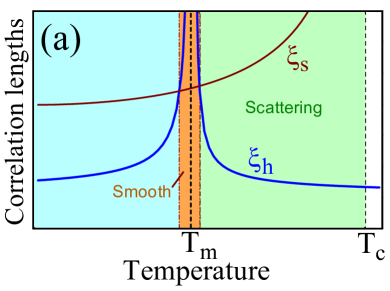
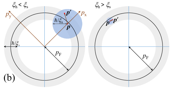
Figure 1: (a)Schematic temperature dependences of the magnetic correlation length $\xi_{h}$ and superconducting coherence length $\xi_{s}$. The influence of the fluctuating magnetic moments on superconductivity is very different in the regions $\xi_{h}>\xi_{s}$ and $\xi_{h}<\xi_{s}$. (b)Typical scales in momentum space characterizing scattering on magnetic fluctuations for two relations between $\xi_{h}$ and $\xi_{s}$ in the case $\xi_{h}\gg k_{F}^{-1}$ with $\hbar k_{F}=p_{F}$. The small circle illustrates the small-angle scattering on magnetic fluctuations with the range $\left|\boldsymbol{p}-\boldsymbol{p}^{\prime}\right|\sim\hbar/\xi_{h}$ and the ring with width $\hbar/\xi_{s}$ illustrate the range relevant for superconductivity.

II Model

We consider a layered material composed of superconducting and magnetic layers described by the Hamiltonian

$$\mathcal{H}=\hat{\mathcal{H}}_{\mathrm{S}}+\hat{\mathcal{H}}_{\mathrm{M}}+\hat{\mathcal{H}}_{\mathrm{MS}},$$ (1)

where

$$\hat{\mathcal{H}}_{\mathrm{S}} =\sum_{n,\mathbf{p}_{\parallel},\sigma}\xi_{\mathrm{2D}}(\mathbf{p}_{\parallel})a_{n,\sigma}^{\dagger}(\mathbf{p}_{\parallel})a_{n,\sigma}(\mathbf{p}_{\parallel})$$

$$+ \!\sum_{n,\mathbf{p}_{\parallel},\sigma}\!t_{\bot}\left[a_{n+1,\sigma}^{\dagger}(\mathbf{p}_{\parallel})a_{n,\sigma}(\mathbf{p}_{\parallel})\!+\!a_{n-1,\sigma}^{\dagger}(\mathbf{p}_{\parallel})a_{n,\sigma}(\mathbf{p}_{\parallel})\right]$$

$$- \sum_{n,\mathbf{p}_{\parallel}}\left[\Delta a_{n,\uparrow}^{\dagger}(\mathbf{p}_{\parallel})a_{n,\downarrow}^{\dagger}(-\mathbf{p}_{\parallel})\!+\!\Delta^{\ast}a_{n,\downarrow}(-\mathbf{p}_{\parallel})a_{n,\uparrow}(\mathbf{p}_{\parallel})\right]$$ (2)

is the standard BCS Hamiltonian describing a layered superconductor. Here $\sigma$ is spin index, $\xi_{\mathrm{2D}}(\mathbf{p}_{\parallel})=\varepsilon_{\mathrm{2D}}(\mathbf{p}_{\parallel})-\mu$ is the single-layer spectrum, $t_{\bot}$ is the interlayer hopping integral, and $\Delta$ is the superconducting gap. The full 3D spectrum for this model is $\xi_{\mathbf{p}}\!=\!\xi_{\mathrm{2D}}(\mathbf{p}_{\parallel})\!+\!2t_{\bot}\cos\left(p_{z}s\right)$. However, its exact shape has a very little effect on further consideration. The second term, $\hat{\mathcal{H}}_{\mathrm{M}}$, describes the quasi-two-dimensional magnetic subsystem leading to a continuous phase transition at $T_{m}$. The last term

$$\hat{\mathcal{H}}_{\mathrm{MS}}\!=\!\!\sum_{n,m,\mathbf{R}}\!\int\!\!d^{2}\boldsymbol{r}J_{nm}\!\left(\mathbf{r}\!-\!\mathbf{R}\right)\mathbf{S}_{m}(\mathbf{R})\hat{\mathbf{\boldsymbol{\sigma}}}_{\alpha\beta}a_{n,\alpha}^{\dagger}(\mathbf{r})a_{n,\beta}(\mathbf{r})$$ (3)

describes the interaction between the magnetic and superconducting layers with the strength set by the nonlocal exchange constants $J_{nm}\left(\mathbf{r}\!-\!\mathbf{R}\right)$. Here the index $m$ marks magnetic layers, $\hat{\mathbf{\boldsymbol{\sigma}}}$ is Pauli-matrix vector, and summation is assumed over the spin indices $\alpha$ and $\beta$. We can rewrite the interaction term as

$$\hat{\mathcal{H}}_{\mathrm{MS}}\!=\!-\!\sum_{n}\int d^{2}\boldsymbol{r}a_{n,\alpha}^{\dagger}(\boldsymbol{r})\boldsymbol{h}_{n}(\boldsymbol{r})\hat{\boldsymbol{\sigma}}_{\alpha\beta}a_{n,\beta}(\boldsymbol{r}),$$ (4)

where

$$\boldsymbol{h}_{n}(\boldsymbol{r})\!=\!-\!\sum_{m,\boldsymbol{R}}J_{nm}(\boldsymbol{r}\!-\!\boldsymbol{R})\boldsymbol{S}_{m}(\boldsymbol{R})$$ (5)

is the effective exchange field acting on spins of conducting electrons. It can be split into the average part $\bar{\boldsymbol{h}}$ due to either polarization of the moments by the magnetic field or spontaneous magnetization in the ordered state and the fluctuating part $\tilde{\boldsymbol{h}}_{n}(\boldsymbol{r})$, $\boldsymbol{h}_{n}(\boldsymbol{r})=\bar{\boldsymbol{h}}+\tilde{\boldsymbol{h}}_{n}(\boldsymbol{r})$,

$$\bar{\boldsymbol{h}} =-\sum_{m,\boldsymbol{R}}J_{nm}(\boldsymbol{r}-\boldsymbol{R})\boldsymbol{\bar{S}},$$ (6a)

$$\tilde{\boldsymbol{h}}_{n}(\boldsymbol{r}) =-\sum_{m,\boldsymbol{R}}J_{nm}(\boldsymbol{r}-\boldsymbol{R})\tilde{\boldsymbol{S}}_{m}(\boldsymbol{R}).$$ (6b)

The fluctuating part of the exchange field also depends on time. We assume that the time scales of magnetic fluctuations exceeds time scales relevant for superconductivity and employ the quasistatic approximation. This assumption is justified near the transition due to the critical slowing down. The fluctuating part is characterized by the correlation function

$$\left\langle\tilde{\boldsymbol{h}}_{n}(\boldsymbol{r})\tilde{\boldsymbol{h}}_{n^{\prime}}(\boldsymbol{r}^{\prime})\right\rangle$$ (7)

$$=\!\!\sum_{m,\boldsymbol{R},\boldsymbol{R}^{\prime}}J_{nm}(\boldsymbol{r}\!-\!\boldsymbol{R})J_{n^{\prime}m}(\boldsymbol{r}^{\prime}\!-\!\boldsymbol{R}^{\prime})\left\langle\tilde{\boldsymbol{S}}_{m}(\boldsymbol{R})\tilde{\boldsymbol{S}}_{m}(\boldsymbol{R}^{\prime})\right\rangle.$$

Here we neglected correlations between different magnetic layers. In the following, we limit ourselves to the case when the uniform field, $\bar{\boldsymbol{h}}$, can be neglected. This corresponds to the paramagnetic state and ordered state near the transition in the absence of an external magnetic field. We will also neglect correlations between different conducting layers and drop the layer index, $\left\langle\tilde{\boldsymbol{h}}_{n}(\boldsymbol{r})\tilde{\boldsymbol{h}}_{n^{\prime}}(\boldsymbol{r}^{\prime})\right\rangle\rightarrow\delta_{n,n^{\prime}}\left\langle\tilde{\boldsymbol{h}}(\boldsymbol{r})\tilde{\boldsymbol{h}}(\boldsymbol{r}^{\prime})\right\rangle$. This corresponds to the two-dimensional approximation for magnetic fluctuations. The spin correlation function is related to the nonlocal spin susceptibility $\chi(\boldsymbol{r}-\boldsymbol{r}^{\prime})$. Sufficiently close to the magnetic transition, the spin correlation length exceeds the range of $J_{nm}(\boldsymbol{r}-\boldsymbol{R})$ and we can approximate

$$\left\langle\tilde{\boldsymbol{h}}(\boldsymbol{r})\tilde{\boldsymbol{h}}(\boldsymbol{r}^{\prime})\right\rangle\approx\sum_{m}\mathcal{J}_{nm}^{2}\left\langle\tilde{\boldsymbol{S}}_{m}(\boldsymbol{r})\tilde{\boldsymbol{S}}_{m}(\boldsymbol{r}^{\prime})\right\rangle.$$ (8)

with $\mathcal{J}_{nm}=\sum_{\boldsymbol{R}}J_{nm}(\boldsymbol{r}-\boldsymbol{R})$. Away from the transition, however, the nonlocality of the exchange interaction may have substantial influence on the amplitude and extent of the exchange-field correlations. We neglect these complications and assume the simplest shape of the correlation function of $\tilde{\boldsymbol{h}}(\boldsymbol{r})$ defined by a single length scale, the in-plane magnetic correlation length $\xi_{h}$,

$$\left\langle\tilde{h}_{\alpha}(\boldsymbol{r})\tilde{h}_{\beta}(\boldsymbol{r}^{\prime})\right\rangle =\frac{h_{0}^{2}}{2}\delta_{\alpha\beta}f_{h}\left(\left|\boldsymbol{r}\!-\!\boldsymbol{r}^{\prime}\right|/\xi_{h}\right),$$ (9)

where $f_{h}(0)\!=\!1$, and the parameter $h_{0}^{2}\!=\!\left\langle\tilde{\boldsymbol{h}}^{2}\right\rangle\!\approx\!\sum_{m}\mathcal{J}_{nm}^{2}\left\langle\tilde{\boldsymbol{S}}^{2}\right\rangle$ weakly depends on temperature. The Fourier transform of the correlation function is

$$\left\langle\left|\tilde{\boldsymbol{h}}_{\mathbf{\mathbf{q}}}\right|^{2}\right\rangle \!=\!sh_{0}^{2}\int\!d^{2}\boldsymbol{r}f_{h}\left(\frac{r}{\xi_{h}}\right)\exp\left(i\boldsymbol{qr}\right)\!=\!sh_{0}^{2}\xi_{h}^{2}\tilde{f}_{h}\left(\xi_{h}q\right).$$ (10)

Here we assume a conventional Lorentz shape for the $q$ dependence, $\tilde{f}_{h}\left(\xi_{h}q\right)\!=\!C_{h}/\left(1\!+\!\xi_{h}^{2}q^{2}\right)$ with $C_{h}\!=\!2\pi\int_{0}^{\infty}\!f_{h}\left(x\right)xdx$. In real space, this corresponds to

$$f_{h}\left(\frac{r}{\xi_{h}}\right)\!=\!\xi_{h}^{2}\!\int\!\frac{d^{2}\boldsymbol{q}}{(2\pi)^{2}}\frac{C_{h}}{1\!+\!\xi_{h}^{2}q^{2}}\exp(i\boldsymbol{qr})\!=\!\frac{C_{h}}{2\pi}K_{0}\left(\frac{r}{\xi_{h}}\right).$$ (11)

The logarithmic divergency $K_{0}(r/\xi_{h})\!\propto\!\ln\left(\xi_{h}/r\right)$ has to be terminated at the distance between neighboring moments $r\!\sim\!a$ . Since the function $f_{h}\left(r/\xi_{h}\right)$ is normalized by the condition $f_{h}(0)=1$, this means that $C_{h}\!\approx\!2\pi/\ln\left(\xi_{h}/a\right)$.

We will utilize the Green’s functions formulation of the superconductivity theory [28, 29]. For investigation of scattering by the magnetic fluctuations, we have to operate with the matrix $4\times 4$ Green’s function[3],

$$\hat{G}(1,2)=-\begin{pmatrix}\left\langle T_{\tau}a_{\alpha}^{\dagger}(1)a_{\beta}(2)\right\rangle&\left\langle T_{\tau}a_{\alpha}(1)a_{\beta}(2)\right\rangle\\ \left\langle T_{\tau}a_{\alpha}^{\dagger}(1)a_{\beta}^{\dagger}(2)\right\rangle&\left\langle T_{\tau}a_{\alpha}(1)a_{\beta}^{\dagger}(2)\right\rangle\end{pmatrix}.$$

We will expand it with respect to the fluctuating exchange field. The unperturbed Green’s function can be written as

$$\hat{G}_{0} =-\frac{\left(i\omega_{n}\hat{\tau}_{0}+\xi_{\mathbf{p}}\hat{\tau}_{z}\right)\hat{\sigma}_{0}-\Delta\hat{\sigma}_{y}\hat{\tau}_{y}}{\omega_{n}^{2}+\xi_{\mathbf{p}}^{2}+\Delta^{2}}$$ (12)

where $\hat{\sigma}_{a}$ and $\hat{\tau}_{b}$ are the Pauli matrices in the spin and Nambu space, respectively. We see that the unperturbed Green’s function can be expanded as $\hat{G}=\sum_{ab}\hat{\sigma}_{a}\hat{\tau}_{b}G_{ab}$ and, without the uniform exchange field, the only nonzero components are $00$, $0z$, and $yy$. For the single-band BCS model, the gap equation is

$$\Delta=UT\sum_{\omega_{n}}\int\frac{d^{3}\mathbf{p}}{(2\pi)^{3}}G_{yy}(\mathbf{p}),$$ (13)

where $U$ is the pairing interaction.

III Scattering by fluctuating exchange field

The Green’s function renormalized by scattering is

$$\hat{G}^{-1} =\hat{G}_{0}^{-1}-\hat{\Sigma}$$ (14)

where $\hat{G}_{0}^{-1}\!=i\omega_{n}\hat{\sigma}_{0}\hat{\tau}_{0}\!-\xi_{\mathbf{p}}\hat{\sigma}_{0}\hat{\tau}_{z}\!+\Delta\hat{\sigma}_{y}\hat{\tau}_{y}$ and

$$\hat{\Sigma}(\mathbf{p})=\int\frac{d^{3}\mathbf{q}}{(2\pi)^{3}}\left\langle\left|\tilde{h}_{\boldsymbol{q},i}\right|^{2}\right\rangle\hat{\alpha}_{i}\hat{G}(\mathbf{p}+\mathbf{q})\hat{\alpha}_{i}$$ (15)

is the self-energy due to the scattering on the fluctuating exchange field with $\hat{\boldsymbol{\alpha}}=\left(\hat{\tau}_{z}\hat{\sigma}_{x},\hat{\tau}_{0}\hat{\sigma}_{y},\hat{\tau}_{z}\hat{\sigma}_{z}\right)$[3]. Using the expansion $\hat{\Sigma}(\mathbf{p})=\sum_{a,b}\Sigma_{ab}\hat{\sigma}_{a}\hat{\tau}_{b}$, we obtain that the relevant components with $ab=00,\,0z,\,yy$ are

$$\Sigma_{ab}(\mathbf{p}) =\int\frac{d^{3}\mathbf{\mathbf{p}^{\prime}}}{(2\pi)^{3}}\left\langle\left|\tilde{\boldsymbol{h}}_{\boldsymbol{p}-\mathbf{p}^{\prime}}\right|^{2}\right\rangle G_{ab}(\mathbf{p}^{\prime}).$$

with

$$\Sigma_{00}(\mathbf{p}) =-\int\frac{d^{3}\mathbf{p}^{\prime}}{(2\pi)^{3}}\left\langle\left|\tilde{\boldsymbol{h}}_{\boldsymbol{p}-\boldsymbol{p}^{\prime}}\right|^{2}\right\rangle\frac{i\omega_{n}}{\omega_{n}^{2}+\xi_{\mathbf{p}^{\prime}}^{2}+\Delta^{2}},$$ (16a)

$$\Sigma_{0z}(\mathbf{p}) =-\int\frac{d^{3}\mathbf{p}^{\prime}}{(2\pi)^{3}}\left\langle\left|\tilde{\boldsymbol{h}}_{\boldsymbol{p}-\boldsymbol{p}^{\prime}}\right|^{2}\right\rangle\frac{\xi_{\mathbf{p}^{\prime}}}{\omega_{n}^{2}+\xi_{\mathbf{p}^{\prime}}^{2}+\Delta^{2}},$$ (16b)

and $\Sigma_{yy}(\mathbf{p})=-\frac{\Delta}{i\omega_{n}}\Sigma_{00}(\mathbf{p})$.

The behavior of $\hat{\Sigma}_{\mathbf{p}}$ depends on the relation between three length scales: the magnetic correlation length $\xi_{h}$, in-plane coherence length $\xi_{s}$, and inverse Fermi wave vector $k_{F}^{-1}$. Consider first limiting cases qualitatively. For very long correlations $\xi_{h}>\xi_{s}$, we have a slowly varying exchange field. In this case, we can neglect $\mathbf{p}^{\prime}$ dependence everywhere except $\langle|\tilde{\boldsymbol{h}}_{\boldsymbol{p}-\boldsymbol{p}^{\prime}}|^{2}\rangle$ giving

$$\hat{\Sigma}(\mathbf{p}) \approx h_{0}^{2}\hat{G}_{0}(\mathbf{p}).$$ (17)

This corresponds to the correction due to the uniform exchange field equal to $h_{0}$ averaged over its directions. We make two observations from this simple result, which will be essential in the further consideration: (i) $\hat{\Sigma}(\mathbf{p})$ has the same nonzero components as $\hat{G}_{0}(\mathbf{p})$, i.e., $00$, $yy$, and $0z$ and (ii) the momentum dependence in $\hat{\Sigma}(\mathbf{p})$ can not be neglected.

In the case $\xi_{h}\!<\!\xi_{s}$, we can integrate over $\xi_{\mathbf{p}^{\prime}}$ and obtain the well-known Abrikosov-Gor’kov magnetic-scattering result [1],

$$\hat{\Sigma}(\mathbf{p}) \approx\frac{1}{2\tau_{m}}\frac{-i\omega_{n}\hat{\sigma}_{0}\hat{\tau}_{0}+\Delta\hat{\sigma}_{y}\hat{\tau}_{y}}{\sqrt{\omega_{n}^{2}+\Delta^{2}}}$$ (18)

with the scattering rate

$$\frac{1}{2\tau_{m}} =\int\frac{\pi dS_{F}^{\prime}}{(2\pi)^{3}v_{F}^{\prime}}\left\langle\left|\tilde{\boldsymbol{h}}_{\boldsymbol{p}-\boldsymbol{p}^{\prime}}\right|^{2}\right\rangle,$$ (19)

which accounts for possibility that the range of $\langle|\tilde{\boldsymbol{h}}_{\boldsymbol{p}-\boldsymbol{p}^{\prime}}|^{2}\rangle$ may be much smaller than the Fermi-surface size[18]. Note that, in contrast to the case of long correlations, Eq. (17), (i) the $\boldsymbol{p}$ dependence of $\hat{\Sigma}(\mathbf{p})$ in Eq. (18) can be neglected and (ii)$\Sigma_{0z}$ component can be omitted. These are standard approximations of the AG theory. In the regime $\xi_{h}>k_{F}^{-1}$ the magnetic fluctuations give small-angle scattering, see illustration in Fig. 1(b). The dependence of the scattering rate on the correlation length following from Eq. (19) is sensitive to the dimensionality of scattering. For three-dimensional scattering, the scattering rate increases logarithmically with $\xi_{h}$ [18]. In our quasi-2D case, we assume that scattering occurs in the whole range of $p_{z}-p_{z}^{\prime}$ but with small change of the in-plane momentum. In this case Eq. (19) gives

$$\frac{1}{2\tau_{m}}=\frac{2\pi}{s}\int\limits_{-\infty}^{\infty}\frac{\pi dq}{(2\pi)^{3}v_{F}}\frac{C_{h}sh_{0}^{2}\xi_{h}^{2}}{1+\xi_{h}^{2}q^{2}}=\frac{C_{h}h_{0}^{2}\xi_{h}}{4v_{F}}.$$ (20)

In general case, the product $C_{h}h_{0}^{2}\xi_{h}$ in this formula and in several results below, can be directly computed from the correlation function of the exchange field as

$$C_{h}h_{0}^{2}\xi_{h}=\int_{0}^{\infty}dr\left\langle\tilde{\boldsymbol{h}}(r)\tilde{\boldsymbol{h}}(0)\right\rangle.$$ (21)

This relation allows evaluation of the scattering rate from the spin-spin correlation function, see Eq. (8), which can be computed for a particular magnetic model. We can see that in the quasi-2D case the scattering rate increases linearly with $\xi_{h}$, much faster than in the 3D case [18]. For completeness, we also present here the result for very short correlation $\xi_{h}k_{F}<1$ when magnetic fluctuations scatter at all angles. In this case we can replace $|\tilde{\boldsymbol{h}}_{\boldsymbol{p}-\boldsymbol{p}^{\prime}}|^{2}$ with $|\tilde{\boldsymbol{h}}_{0}|^{2}$and obtain the Abrikosov-Gor’kov result for uncorrelated magnetic impurities

$$\frac{1}{2\tau_{m}}=C_{h}\nu h_{0}^{2}s\xi_{h}^{2},$$ (22)

where $\nu$ is the density of states. In particular, for quasi-2D electronic spectrum $\nu=m/(2\pi\hbar^{2}s)$ where $m$ is the effective mass.

Away from the magnetic transition, the magnetic correlation length $\xi_{h}$ is of the order of separation between the magnetic moments $a$. For a continuous magnetic transition inside the superconducting state, the magnetic correlation length rapidly increases for $T\rightarrow T_{m}$ and at some point exceeds the coherence length. At this crossover the impact of magnetic fluctuations on superconductivity modifies qualitatively. We now quantify the crossover between the regimes $\xi_{h}>\xi_{s}$, Eq. (17), and $\xi_{h}<\xi_{s}$, Eqs. (18) and (20). It is important to note that in the second (scattering) regime only two components of $\hat{\Sigma}$ are essential, $00$ and $yy$. In the first regime, however, also the $0z$ component describing spectrum renormalization has to be included. The latter component obviously also has to be taken into account in the description of the crossover. First, we consider the $00$ component (the $00$ and $yy$ components are related as $\Sigma_{yy}=-\frac{\Delta}{i\omega_{n}}\Sigma_{00}$). As the scattering in the regime $k_{F}\xi_{h}\gg$1 is small angle, we need to consider only a small region at the Fermi surface near the initial momentum $\boldsymbol{p}$. Selecting the $x$ axis along this momentum and $y$ axis in the perpendicular direction [see Fig. 1(b)] and using $\langle|\tilde{\boldsymbol{h}}_{\mathbf{\mathbf{q}}}|^{2}\rangle$ in Eq. (10), we transform Eq. (16a) as

$$\Sigma_{00}(\mathbf{p}) =\!-\!\int\frac{dp_{x}^{\prime}dp_{y}^{\prime}}{(2\pi)^{2}}\frac{C_{h}h_{0}^{2}\xi_{h}^{2}}{1\!+\!\xi_{h}^{2}\left(p_{x}^{\prime}\!-\!p_{x}\right)^{2}\!+\!\xi_{h}^{2}p_{y}^{\prime}{}^{2}}$$

$$\times \frac{i\omega_{n}}{\omega_{n}^{2}\!+\!v_{F}^{2}\left(p_{x}^{\prime}\!-\!p_{F}\right)^{2}\!+\!\Delta^{2}}.$$ (23)

Integrating with respect to $p_{y}^{\prime}$, we obtain

$$\Sigma_{00}(\mathbf{p}) =-\frac{C_{h}h_{0}^{2}\xi_{h}}{4\pi}\int_{-\infty}^{\infty}dp_{x}^{\prime}\frac{1}{\sqrt{1+\xi_{h}^{2}{p_{x}^{\prime}}^{2}}}$$

$$\times \frac{i\omega_{n}}{\omega_{n}^{2}\!+\!v_{F}^{2}\left(p_{x}^{\prime}\!+\!\delta p_{x}\right)^{2}\!+\!\Delta^{2}}$$

$$=-\frac{C_{h}h_{0}^{2}}{4\pi}\frac{i\omega_{n}}{\omega_{n}^{2}+\Delta^{2}}U\left(\delta k_{x},g_{n}\right),$$ (24)

where $\delta p_{x}=p_{x}-p_{F}$,

$$g_{n}=\frac{v_{F}/\xi_{h}}{\sqrt{\omega_{n}^{2}\!+\!\Delta^{2}}},\,\delta k_{x}=\!\frac{v_{F}\left(p_{x}\!-\!p_{F}\right)}{\sqrt{\omega_{n}^{2}+\Delta^{2}}}=\!\frac{\xi_{p}}{\sqrt{\omega_{n}^{2}\!+\!\Delta^{2}}},$$ (25)

and the reduced function $U\left(k,g\right)$ is defined by the integral

$$U\left(k,g\right)=\int\limits_{-\infty}^{\infty}du\frac{1}{\sqrt{1+u^{2}}}\frac{1}{1+\left(gu+k\right)^{2}},$$

which can be taken analytically giving

$$U\left(k,g\right) =\mathrm{Re}\left[W\left(k,g\right)\right],$$ (26)

$$W\left(k,g\right) =\!\frac{2}{\sqrt{\left(ik\!+\!1\right)^{2}\!-\!g^{2}}}\ln\!\left(\frac{ik\!+\!1\!+\!\sqrt{\left(ik\!+\!1\right)^{2}\!-\!g^{2}}}{g}\right).$$

We note that the $k$ dependence of the function $U\left(k,g\right)$ corresponding to the $\xi_{p}$ dependence of the self energy is essential only for $g\lesssim 1$. The value of the function $U\left(k,g\right)$ at $k=0$ has the simple analytical form

$$U\left(0,g\right) =\begin{cases}\frac{2}{\sqrt{1-g^{2}}}\ln\frac{1+\sqrt{1-g^{2}}}{g}&\mathrm{for}\>g<1\\ \frac{2}{\sqrt{g^{2}-1}}\arctan\sqrt{g^{2}-1}&\mathrm{for}\>g>1\end{cases}.$$

The asymptotic $U\left(0,g\right)\simeq\pi/g$ for $g\gg 1$ corresponds the scattering regime, Eqs. (18) and (20). In this limit the $k$ dependence of the function $U\left(k,g\right)$ can be neglected. On the other hand, the asymptotic for $g\ll 1$ is

$$U\left(k,g\right)\simeq 2\left[\frac{1}{1\!+\!k^{2}}\ln\left(2\frac{\sqrt{1\!+\!k^{2}}}{g}\right)+\frac{k}{1\!+\!k^{2}}\arctan k\right].$$

It corresponds to the uniform-field result in Eq. (17) only for the main logarithmic term. Additional terms appear because the correlation function $\langle\tilde{h}_{\alpha}(\boldsymbol{r})\tilde{h}_{\beta}(\boldsymbol{r}^{\prime})\rangle$ in Eq. (9) is not a constant at $|\boldsymbol{r}-\boldsymbol{r}^{\prime}|\!<\!\xi_{h}$ but increases logarithmically as $\ln\left(\xi_{h}/|\boldsymbol{r}-\boldsymbol{r}^{\prime}|\right)$.

As mentioned above, for the proper description of the crossover at $\xi_{h}\sim\xi_{s}$, we also need to take into account the $0z$ component of the self energy,

$$\Sigma_{0z}(\mathbf{p}) =\!-\!\int\frac{dp_{x}^{\prime}dp_{y}^{\prime}}{(2\pi)^{2}}\frac{C_{h}h_{0}^{2}\xi_{h}^{2}}{1\!+\!\xi_{h}^{2}\left(p_{x}^{\prime}\!-\!p_{x}\right)^{2}\!+\!\xi_{h}^{2}p_{y}^{\prime}{}^{2}}$$

$$\times \frac{v_{F}\left(p_{x}^{\prime}-p_{F}\right)}{\omega_{n}^{2}\!+\!v_{F}^{2}\left(p_{x}^{\prime}\!-\!p_{F}\right)^{2}\!+\!\Delta^{2}}.$$ (27)

Following the same route as in derivation of Eq. (24), we present it as

$$\Sigma_{0z}(\mathbf{p}) =-\frac{C_{h}h_{0}^{2}}{4\pi}\frac{1}{\sqrt{\omega_{n}^{2}+\Delta^{2}}}V\left(\delta k_{x},g_{n}\right),$$ (28)

where the parameters $g_{n}$ and $\delta k_{x}$ are defined in Eq. (25),

$$V\left(k,g\right)\!=\!\int\limits_{-\infty}^{\infty}\!du\frac{1}{\sqrt{1\!+\!u^{2}}}\frac{gu+k}{1\!+\!\left(gu\!+\!k\right)^{2}}=\!-\mathrm{Im}\left[W\left(k,g\right)\right],$$ (29)

and the function $W\left(k,g\right)$ is defined in Eq. (26). In particular, for $g\rightarrow 0$

$$V\left(k,g\right)\simeq\frac{2}{1+k^{2}}\left[k\ln\left(\frac{2}{g}\right)-\arctan k\right].$$

As follows from Eq. (14), the renormalized Green’s function can be obtained by substitutions $i\omega_{n}\rightarrow i\tilde{\omega}_{n}=i\omega_{n}-\Sigma_{00}$, $\Delta\rightarrow\tilde{\Delta}=\Delta-\Sigma_{yy}$, and $\xi_{\mathbf{p}}\rightarrow\tilde{\xi}_{\mathbf{p}}=\xi_{\mathbf{p}}+\Sigma_{0z}$. The renormalized frequency, gap, and spectrum can be written as

$$\tilde{\omega}_{n}=\omega_{n}(1+\alpha_{n}),\,\tilde{\Delta}=\Delta_{0}(1-\alpha_{n}),\,\tilde{\xi}_{\mathbf{p}}=\xi_{\mathbf{p}}(1-\beta_{n})$$ (30)

with

$$\alpha_{n}=\frac{C_{h}h_{0}^{2}}{4\pi}\frac{U\left(\delta k_{x},g_{n}\right)}{\omega_{n}^{2}+\Delta_{0}^{2}},\ \beta_{n}=\frac{C_{h}h_{0}^{2}}{4\pi}\frac{V\left(\delta k_{x},g_{n}\right)/\xi_{\mathbf{p}}}{\sqrt{\omega_{n}^{2}+\Delta_{0}^{2}}}.$$ (31)

With derived results for the self-energy in Eqs. (24) and (28), we proceed with evaluation of correction to the gap parameter from Eq. (13).

IV Correction to the gap

The superconducting gap is the most natural parameter characterizing the strength of superconductivity at a given temperature. In this section, we calculate the suppression of this parameter by correlated magnetic fluctuations. The key observation is that a small uniform exchange field has no influence on the gap at zero temperature [19]. Therefore, one can expect that the suppression caused by correlated magnetic fluctuations at low temperatures diminishes when the magnetic correlation length exceeds the superconducting coherence length.

The gap equation in Eq. (13) is determined by the integral

$$\mathcal{I}=\int\frac{d^{3}\mathbf{p}}{(2\pi)^{3}}G_{yy}(\mathbf{p})=\nu\int_{-\infty}^{\infty}d\xi\frac{\tilde{\Delta}}{\tilde{\omega}_{n}^{2}\!+\!\tilde{\xi}^{2}\!+\!\tilde{\Delta}^{2}},$$ (32)

where the parameters with “$\sim$” are defined in Eqs. (30) and (31). We evaluate the linear correction to $\mathcal{I}$ with respect to $\alpha_{n},\beta_{n}\propto h_{0}^{2}$ as

$$\mathcal{\delta I} =-\nu\int\limits_{-\infty}^{\infty}\!d\xi\frac{\Delta_{0}}{\omega_{n}^{2}\!+\!\xi^{2}\!+\!\Delta_{0}^{2}}$$

$$\times \left(\alpha_{n}\!+\!\frac{2\alpha_{n}\left(\omega_{n}^{2}\!-\!\Delta_{0}^{2}\right)\!-\!2\beta_{n}\xi^{2}}{\left(\omega_{n}^{2}+\xi^{2}+\Delta_{0}^{2}\right)}\right).$$

Making the substitution $\xi=z\sqrt{\omega_{n}^{2}+\Delta_{0}^{2}}$, we transform this correction to the following form

$$\delta\mathcal{I} =-\frac{C_{h}\nu h_{0}^{2}}{4\pi}\frac{\Delta_{0}}{\left(\omega_{n}^{2}+\Delta_{0}^{2}\right)^{3/2}}$$

$$\times \mathrm{Re}\left[\int\limits_{-\infty}^{\infty}dz\frac{W\left(z,g_{n}\right)\left(\left(z-i\right)^{2}+\frac{4\omega_{n}^{2}}{\omega_{n}^{2}+\Delta_{0}^{2}}\right)}{\left(z^{2}+1\right)^{2}}\right].$$ (33)

Calculation of the integral described in appendix A yields the result

$$\delta\mathcal{I} =-C_{h}\nu h_{0}^{2}\frac{\Delta_{0}}{\left(\omega_{n}^{2}+\Delta_{0}^{2}\right)^{5/2}}\left\{\frac{\Delta_{0}^{2}}{4-g_{n}^{2}}\right.$$

$$+ \left.\frac{\omega_{n}^{2}\left(4\!-\!g_{n}^{2}\right)\!-\!2\Delta_{0}^{2}}{\left(4-g_{n}^{2}\right)^{3/2}}\ln\left(\frac{2\!+\!\sqrt{4\!-\!g_{n}^{2}}}{g_{n}}\right)\right\}.$$ (34)

The corrected equation for the gap $\Delta=UT\sum_{\omega_{n}}(\mathcal{I}_{0}+\delta\mathcal{I})$ with $\mathcal{I}_{0}=\pi/\sqrt{\omega_{n}^{2}+\Delta_{0}^{2}}$ gives the gap correction caused by the nonuniform exchange field

$$\tilde{\Delta} =-C_{h}h_{0}^{2}T\!\sum_{\omega_{n}}\!\frac{1}{\left(\omega_{n}^{2}\!+\!\Delta_{0}^{2}\right)^{5/2}}.$$

$$\times \mathrm{Re}\!\left[\frac{\Delta_{0}^{2}}{4\!-\!g_{n}^{2}}\!+\!\frac{4\omega_{n}^{2}\!-\!2\Delta_{0}^{2}\!-\!\omega_{n}^{2}g_{n}^{2}}{\left(4-g_{n}^{2}\right)^{3/2}}\ln\!\left(\!\frac{2\!+\!\sqrt{4\!-\!g_{n}^{2}}}{g_{n}}\!\right)\!\right]$$

$$\times \left[\pi T\!\sum_{\omega_{n}}\frac{\Delta_{0}}{\left(\omega_{n}^{2}\!+\!\Delta_{0}^{2}\right)^{3/2}}\right]^{-1}.$$

Substituting the definition of $g_{n}$ in Eq. (25), we finally obtain

$$\tilde{\Delta} =\!-\left[\pi T\sum_{\omega_{n}}\frac{\Delta_{0}}{\varOmega_{n}^{3}}\right]^{-1}\!C_{h}h_{0}^{2}T\sum_{\omega_{n}}\frac{1}{\varOmega_{n}^{3}\left(4\varOmega_{n}^{2}-\varepsilon_{h}^{2}\right)}$$ (35)

$$\times \!\left[\!\Delta_{0}^{2}\!+\!\frac{2\left(2\omega_{n}^{2}\!-\!\Delta_{0}^{2}\right)\varOmega_{n}^{2}\!-\!\omega_{n}^{2}\varepsilon_{h}^{2}}{\varOmega_{n}\sqrt{4\varOmega_{n}^{2}-\varepsilon_{h}^{2}}}\ln\!\left(\!\frac{2\varOmega_{n}\!+\!\sqrt{4\varOmega_{n}^{2}\!-\!\varepsilon_{h}^{2}}}{\varepsilon_{h}}\right)\!\right]$$

with $\varOmega_{n}=\sqrt{\omega_{n}^{2}\!+\!\Delta_{0}^{2}}$ and the magnetic-scattering energy scale $\varepsilon_{h}\!=\!v_{F}/\xi_{h}$. Introducing the reduced variables

$$\tilde{T}\!= 2\pi T/\Delta_{0}(T),\ \tilde{\omega}_{n}\!=\!\tilde{T}(n\!+\!1/2),$$

$$\alpha_{h}\!= \varepsilon_{h}(T)/2\Delta_{0}(T)\!=\!\xi_{s}(T)/\xi_{h}(T)$$

with $\xi_{s}(T)\!=\!v_{F}/2\Delta_{0}(T)$, and using the estimate $C_{h}\!\approx\!2\pi/\ln\left(\xi_{h}/a\right)$, we rewrite this result in the form convenient for numerical evaluation

$$\tilde{\Delta}(T)= -\frac{h_{0}^{2}}{2\Delta_{0}(T)\ln\left(\xi_{h}(T)/a\right)}\mathcal{V}_{\Delta}\left(\frac{2\pi T}{\Delta_{0}(T)},\frac{\xi_{s}(T)}{\xi_{h}(T)}\right),$$ (36a)

$$\mathcal{V}_{\Delta}\left(\tilde{T},\alpha_{h}\right) =\left[\mathcal{D}(\tilde{T})\right]^{-1}\tilde{T}\sum_{n=0}^{\infty}R\left[\tilde{\omega}_{n},\alpha_{h}\right],$$ (36b)

$$\mathcal{D}(\tilde{T}) =\tilde{T}\sum_{n=0}^{\infty}\left(\tilde{\omega}_{n}^{2}\!+1\right)^{-3/2},$$ (36c)

$$R\left(z,\alpha_{h}\right) =\frac{1}{\left(z^{2}\!+\!1\right)^{3/2}\left(z^{2}\!+\!1\!-\!\alpha_{h}^{2}\right)}\left[1\!+\!\left(2z^{2}\!-\!1\!-\!\frac{2z^{2}\alpha_{h}^{2}}{z^{2}\!+\!1}\right)\mathit{L}\left(z,\alpha_{h}\right)\right].$$ (36d)

$$\mathit{L}\left(z,\alpha_{h}\right) =\begin{cases}\frac{\sqrt{z^{2}+1}}{\sqrt{z^{2}+1-\alpha_{h}^{2}}}\ln\left(\frac{\sqrt{z^{2}\!+\!1}\!+\!\sqrt{z^{2}\!+\!1\!-\!\alpha_{h}^{2}}}{\alpha_{h}}\right),&z^{2}\!>\!\alpha_{h}^{2}\!-\!1\\ \frac{\sqrt{z^{2}+1}}{\sqrt{\alpha_{h}^{2}-z^{2}-1}}\arctan\frac{\sqrt{\alpha_{h}^{2}\!-\!z^{2}\!-\!1}}{\sqrt{z^{2}\!+\!1}},&z^{2}\!<\!\alpha_{h}^{2}\!-\!1\end{cases}.$$ (36e)

Note that the function $L\left(z,\alpha_{h}\right)$ does not have singularity at $z=\sqrt{\alpha_{h}^{2}-1}$ for $\alpha_{h}>1$, contrary to what its shape may suggest. We see that the gap correction has the amplitude $h_{0}^{2}/\Delta_{0}$ and mostly depends on two dimensionless parameters: reduced temperature $T/\Delta_{0}(T)$ and the ratio $\alpha_{h}\!=\!\xi_{s}(T)/\xi_{h}(T)$. It also weakly depends on the ratio $\xi_{h}/a$, which determines the logarithmic factor in the denominator of Eq. (36a).

Let us discuss asymptotic behavior of the reduced function $\mathcal{V}_{\Delta}(\tilde{T},\alpha_{h})$ and the gap correction it gives. In the range $\alpha_{h}\gg 1$ corresponding to the scattering regime, the function $R\left(z,\alpha_{h}\right)$ in Eq. (36d) behaves as $R\left(z,\alpha_{h}\right)\simeq\frac{\pi z^{2}}{\alpha_{h}\left(z^{2}+1\right)^{2}}$. This gives the following asymptotics of the function $\mathcal{V}_{\Delta}(\tilde{T},\alpha_{h})$

$$\mathcal{V}_{\Delta}\left(\tilde{T},\alpha_{h}\right) \simeq\frac{\pi}{\alpha_{h}}V_{\Delta}(\tilde{T}),$$ (37a)

$$V_{\Delta}(\tilde{T})= \left[\mathcal{D}(\tilde{T})\right]^{-1}\!\tilde{T}\sum_{n=0}^{\infty}\frac{\tilde{\omega}_{n}^{2}}{\left(\tilde{\omega}_{n}^{2}+1\right)^{2}},$$ (37b)

where the limiting behaviors of the function $V_{\Delta}(\tilde{T})$ are $V_{\Delta}(0)\!=\!\pi/4$ and $V_{\Delta}(\tilde{T})\!\simeq\!{\pi^{2}\tilde{T}}/[{14\zeta(3)}]$ for $\tilde{T}\!\gg\!1$ with $\zeta(3)\approx 1.202$. Correspondingly, the correction to the gap in this regime simplifies to

$$\tilde{\Delta}(T)\simeq-\frac{\pi\xi_{h}h_{0}^{2}}{v_{F}\ln\left(\xi_{h}/a\right)}V_{\Delta}(\tilde{T})=-\frac{1}{\tau_{m}}V_{\Delta}(\tilde{T}).$$ (38)

This is a well-known result for the gap correction caused by the magnetic scattering[1, 2].

In the opposite regime $\alpha_{h}\rightarrow 0$ corresponding to the vicinity of the magnetic transition, the function $R\left(z,\alpha_{h}\right)$ has a logarithmic dependence on $\alpha_{h}$

$$R\left(z,\alpha_{h}\right) =R_{0}(z)+R_{1}(z)\ln\left(\frac{1}{\alpha_{h}}\right),$$

$$R_{0}(z)= \frac{1\!+\!\left(2z^{2}\!-\!1\right)\ln\left(2\sqrt{z^{2}\!+\!1}\right)}{\left(z^{2}+1\right)^{5/2}},$$

$$R_{1}(z)= \frac{2z^{2}-1}{\left(z^{2}+1\right)^{5/2}}$$

meaning that $\mathcal{V}_{\Delta}(\tilde{T},\alpha_{h})$ also logarithmically diverges for $\alpha_{h}\rightarrow 0$,

$$\mathcal{V}_{\Delta}\left(\tilde{T},\alpha_{h}\right) =\mathcal{A}(\tilde{T})+\mathcal{B}(\tilde{T})\ln\left(\frac{1}{\alpha_{h}}\right),$$ (39a)

$$\mathcal{A}(\tilde{T}) =\left[\mathcal{D}(\tilde{T})\right]^{-1}\!\tilde{T}\sum_{n=0}^{\infty}\!R_{0}(\tilde{\omega}_{n}),$$ (39b)

$$\mathcal{B}(\tilde{T}) =\left[\mathcal{D}(\tilde{T})\right]^{-1}\tilde{T}\sum_{n=0}^{\infty}R_{1}(\tilde{\omega}_{n})$$ (39c)

with $\mathcal{A}(0)=1$, $\mathcal{B}(0)=0$. The plots of the coefficients $\mathcal{A}(\tilde{T})$ and $\mathcal{B}(\tilde{T})$ are shown in Fig. 2. The corresponding correction to the gap can be presented as

$$\tilde{\Delta}(\tilde{T}) =\!-\frac{h_{0}^{2}\mathcal{B}(\tilde{T})}{2\Delta_{0}}\left[1\!-\frac{\ln\left(\frac{\xi_{s}}{a}\right)\!-\!\mathcal{A}(\tilde{T})\!/\!\mathcal{B}(\tilde{T})}{\ln\left(\xi_{h}/a\right)}\right].$$ (40)

Therefore, the absolute value of correction $|\tilde{\Delta}|$ decreases when $T$ approaches $T_{m}$ if the ratio $\mathcal{A}(\tilde{T}_{m})/\mathcal{B}(\tilde{T}_{m})$ exceeds $\ln\left(\xi_{s}/a\right)$, which always occurs at sufficiently low temperatures, see inset in Fig. 2. In this case the overall dependence of the correction on $\xi_{h}$ is nonmonotonic and maximum suppression of the gap occurs at $\xi_{h}\sim\xi_{s}$. The limiting value at $T=T_{m}$ , $\tilde{\Delta}(\tilde{T}_{m})=-h_{0}^{2}\mathcal{B}(\tilde{T}_{m})/2\Delta_{0}$, corresponds to the correction from a uniform exchange field equal to $h_{0}$. It vanishes for $T_{m}\rightarrow 0$ as $\exp\left(-\Delta_{0}/T_{m}\right)$.

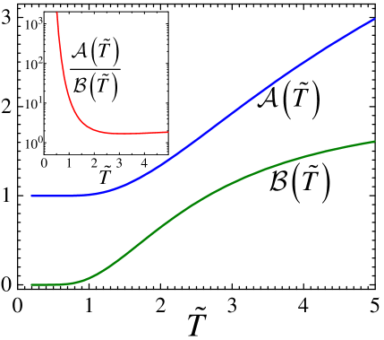
Figure 2: Temperature dependences of the coefficients $\mathcal{A}(\tilde{T})$ and $\mathcal{B}(\tilde{T})$ which determine the small-$\alpha_{h}$ asymptotics of the function $\mathcal{V}_{\Delta}(\tilde{T},\alpha_{h})$ in Eq. (39a). The inset shows the temperature dependence of the ratio $\mathcal{A}(\tilde{T})/\mathcal{B}(\tilde{T})$.

At temperatures much smaller than $T_{c}$, the summation over the Matsubara frequencies in Eq. (36b) can be transformed into integration leading to

$$\tilde{\Delta}(0) =-\frac{h_{0}^{2}}{2\Delta_{0}\ln\left(\xi_{h}/a\right)}\mathcal{V}_{\Delta}\!\left(\frac{\xi_{s}}{\xi_{h}}\right),$$ (41)

where the reduced function $\mathcal{V}_{\Delta}\left(\alpha_{h}\right)\equiv\mathcal{V}_{\Delta}\left(0,\alpha_{h}\right)$ is defined by the integral

$$\mathcal{V}_{\Delta}\left(\alpha_{h}\right) =\int_{0}^{\infty}R\left(z,\alpha_{h}\right)dz.$$

This is a monotonically-decreasing function with the asymptotics

$$\mathcal{V}_{\Delta}\left(\alpha_{h}\right)\!\simeq\!\begin{cases}1\!+\frac{1}{9}(6\ln\alpha_{h}\!+\!1)\alpha_{h}^{2},&\mathrm{for}\,\alpha_{h}\!\ll\!1\\ \frac{\pi^{2}}{4\alpha_{h}}-\frac{2\ln\alpha_{h}+1}{\alpha_{h}^{2}},&\mathrm{for}\,\alpha_{h}\!\gg\!1\end{cases}.$$ (42)

It also has the exact value $\mathcal{V}_{\Delta}(1)=\frac{\pi^{2}}{8}-\frac{1}{2}$. The large-$\alpha_{h}$ asymptotics corresponds to the magnetic-scattering regime[1, 2, 3]. Substituting the first leading term into Eq. (41) yields the known result for the gap correction at zero temperature $\tilde{\Delta}(0)\approx-\pi/4\tau_{m}$, where $\tau_{m}$ is given by Eq. (20).

Plots of the numerically evaluated function $\mathcal{V}_{\Delta}(\tilde{T},\alpha_{h})$ are shown in Fig, 3 for several values of the reduced temperature $\tilde{T}$. The function monotonically decreases with $\alpha_{h}$ and increases with temperature. At zero temperature this function approaches a finite value for $\alpha_{h}\rightarrow 0$ while at finite temperatures it logarithmically diverges, as discussed above. For zero temperature, we also show the scattering-regime dependence by dashed line and more accurate asymptotic presented in Eq. (42) by dotted line. We can see that the scattering approximation noticeably overestimates the gap correction for rather large values of $\alpha_{h}$. The finite value of the function for $\alpha_{h}\rightarrow 0$ at zero temperature is in an apparent contradiction with the known result that a uniform exchange field does not change the gap at zero temperature [19]. This finite value is the consequence of small-distance behavior of the exchange-field correlation function for the two-dimensional case: it does not approach a constant for $r\ll\xi_{h}$ but keeps growing logarithmically, see Eqs. (9) and (11). We note, however, that despite this small-$\alpha_{h}$ saturation of the function $\mathcal{V}_{\Delta}\left(0,\alpha_{h}\right)$, the gap correction in Eq. (36a) does have a nonmonotonic dependence on $\xi_{h}$ and vanishes in the limit $\xi_{h}\rightarrow\infty$ at low temperatures because of the logarithmic factor in the denominator.

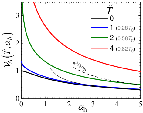
Figure 3: Plots of the function $\mathcal{V}_{\Delta}(\tilde{T},\alpha_{h})$ in Eq. (36b) determining the gap correction caused by nonuniform exchange field on the parameter $\alpha_{h}=\xi_{s}/\xi_{h}$ for several values of the reduced temperature $\tilde{T}=2\pi T/\Delta_{0}$. The corresponding relative temperatures for BCS superconductors are shown in parenthesis. For zero temperature, we also show the scattering-regime asymptotics (dashed line) and more accurate asymptotics presented in Eq. (42) (dotted line).

V Correction to the electromagnetic kernel and London penetration depth

In this section, we investigate the correction to the superconducting current response caused by the exchange interaction with correlated magnetic fluctuations. As in the case of the gap parameter, there are two different regimes depending on the relation between the magnetic correlation length $\xi_{h}$ and superconducting coherence length $\xi_{s}$. Our goal is to quantitatively describe the crossover between these two regimes. The case $\xi_{h}<\xi_{s}$ corresponds to the well-studied magnetic-scattering regime. Influence of magnetic scattering on the electromagnetic kernel, which determines the London penetration depth, was investigated by Skalski et al.[2], see also Ref. [3]. Recently, a very detailed investigation of this problem has been performed within the quasiclassical approach [30]. Most studies, however, have been done for isotropic magnetic scattering. The case of correlated magnetic fluctuation in the regime $k_{F}\xi_{h}\gg 1$ requires a proper accounting for the vertex correction to the kernel which is equivalent to accounting for the reverse scattering events in quasiclassical approach .

The superconducting current response

$$j_{\alpha}(\boldsymbol{q},\omega)=-Q_{\alpha\beta}(\boldsymbol{q},\omega)A_{\beta}(\boldsymbol{q},\omega)$$ (43)

is determined by the electromagnetic kernel $Q_{\alpha\beta}(\boldsymbol{q},\omega)$. In strongly type-II superconductors, the screening of magnetic field is determined by the local static kernel $Q_{\alpha\beta}\!\equiv\!Q_{\alpha\beta}(\boldsymbol{0},0)$. The superfluid density $n_{s}$ introduced in the phenomenological London theory is related to $Q_{\alpha\beta}$ as $Q_{\alpha\beta}\!=\!e^{2}n_{s}/cm_{\alpha\beta}$, where $m_{\alpha\beta}$ is the effective mass tensor. The London penetration depth components $\lambda_{\alpha}$ are related to the static uniform kernel as $Q_{\alpha\alpha}\!=\!c/(4\pi\lambda_{\alpha}^{2})$. In nonmagnetic superconductors the screening length $\tilde{\lambda}_{\alpha}$ is identical to this ’bare’ length $\lambda_{\alpha}$ defined via the electromagnetic kernel. In magnetic superconductors, however, the screening length $\tilde{\lambda}_{\alpha}$ is reduced by the magnetic response of local moments as $\tilde{\lambda}_{\alpha}\!=\!\lambda_{\alpha}/\sqrt{\mu}$, where $\mu$ is the magnetic permeability in the magnetic-field direction [31, 5]. Note that the exchange and magnetic response have opposite influences on the screening length: the former enlarges and the latter reduces it. In the following, we concentrate on the calculation of the bare London penetration depth.

In the Green’s function formalism, the kernel can be evaluated as[3]

$$Q_{\alpha\beta}(\boldsymbol{q},\omega_{\nu}) =\frac{e^{2}n}{cm_{\alpha\beta}}+\frac{e^{2}}{2c}T\sum_{\omega_{n}}\!\int\!\frac{d^{3}\boldsymbol{p}}{(2\pi)^{3}}v_{\alpha}v_{\beta}$$

$$\times \mathrm{Tr}\left[\hat{G}(\boldsymbol{p},\omega_{n})\hat{G}(\boldsymbol{p}\!-\!\boldsymbol{q},\omega_{n}\!-\!\omega_{\nu})\right],$$ (44)

where $n$ is total density and $v_{\alpha}=\partial\xi_{p}/\partial p_{\alpha}$ are the velocity components . In particular, for clean case

$$Q_{\alpha\beta}^{(0)} =\frac{2\pi e^{2}}{c}\nu\left\langle v_{\alpha}v_{\beta}\right\rangle T\sum_{\omega_{n}}\frac{\Delta_{0}^{2}}{\left(\omega_{n}^{2}+\Delta_{0}^{2}\right)^{3/2}}$$ (45)

giving $Q_{\alpha\beta}^{(0)}=2\frac{e^{2}}{c}\nu\left\langle v_{\alpha}v_{\beta}\right\rangle$ at zero temperature.

We first consider the scattering regime, $\xi_{h}\ll\xi_{s}$, within the quasiclassical approximation. The generalization of the isotropic-scattering calculations in Ref. [30] for arbitrary scattering described in Appendix B gives the following result for the correction to $\lambda_{\alpha}^{-2}$ due to the magnetic scattering

$$\lambda_{1\alpha}^{-2}(T)= \!-\!\lambda_{0\alpha}^{-2}(T)\left[\frac{1}{\tau_{m}\Delta_{0}(T)}V_{\lambda,m}\left(\frac{2\pi T}{\Delta_{0}(T)}\right)\right.$$

$$+ \left.\frac{1}{\tau_{m}^{\mathrm{tr}}\Delta_{0}(T)}V_{\lambda,m}^{\mathrm{tr}}\left(\frac{2\pi T}{\Delta_{0}(T)}\right)\right],$$ (46)

with

$$V_{\lambda,m}\!(\tilde{T}) \!=\!\frac{1}{\mathcal{D}(\tilde{T})}\tilde{T}\!\sum_{n=0}^{\infty}\left[\!\frac{2\tilde{\omega}_{n}^{2}\!-\!1}{\left(1\!+\!\tilde{\omega}_{n}^{2}\right)^{5/2}}V_{\Delta}\!(\tilde{T})\!+\!\frac{3\tilde{\omega}_{n}^{2}-1}{\left(1\!+\!\tilde{\omega}_{n}^{2}\right)^{3}}\right],$$ (47)

$$V_{\lambda,m}^{\mathrm{tr}}\!(\tilde{T}) \!=\frac{1}{2\mathcal{D}(\tilde{T})}\tilde{T}\sum_{n=0}^{\infty}\frac{1-\tilde{\omega}_{n}^{2}}{\left(1+\tilde{\omega}_{n}^{2}\right)^{3}},$$ (48)

where the functions $\mathcal{D}(\tilde{T})$ and $V_{\Delta}(\tilde{T})$ are defined in Eqs. (36c) and (37b), respectively. Here $\tau_{m}$ is the magnetic-scattering lifetime, Eqs. (19) and (20), and $\tau_{m}^{\mathrm{tr}}$ is the corresponding transport time,

$$\frac{1}{2\tau_{m}^{\mathrm{tr}}} =\int\frac{\pi dS_{F}^{\prime}}{(2\pi)^{3}v_{F}^{\prime}}\left(1-\frac{\boldsymbol{v}\cdot\boldsymbol{v}^{\prime}}{\left\langle v^{2}\right\rangle}\right)\left\langle\left|\tilde{\boldsymbol{h}}_{\boldsymbol{p}-\boldsymbol{p}^{\prime}}\right|^{2}\right\rangle.$$ (49)

The two terms in Eq. (46) can be referred to as the pair-breaking and transport contributions. In the case we consider, the transport scattering rate is much smaller than the total rate, $1/\tau_{m}^{\mathrm{tr}}\!\sim\!1/\left(\xi_{h}k_{F}\tau_{m}\right)\!\ll\!1/\tau_{m}$, and it does not increase when the temperature approaches the magnetic transition. We point, however, that the contribution from the total scattering rate vanishes at low temperatures, $V_{\lambda,m}(0)\!=\!0$, while the transport contribution remains finite $V_{\lambda,m}^{\mathrm{tr}}(0)\!=\!\pi/16$. Nevertheless, as our main goal is to understand suppression of the superconducting parameters near the magnetic transition, in the following consideration we mostly focus on the behavior of the pair-breaking term proportional to the total scattering rate.

The above results are only valid until $\xi_{h}<\xi_{s}$. We proceed with the consideration of the crossover to the opposite regime, which can not be treated within the quasiclassical approach. The total correction to the electromagnetic kernel is

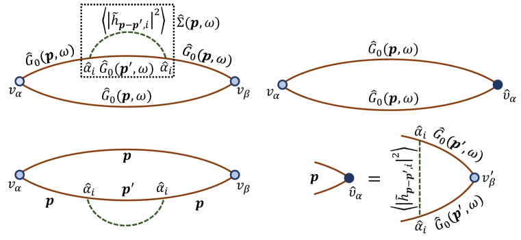
Figure 4: The diagrams for the lowest-order corrections to the electromagnetic kernel caused by the nonuniform exchange field in Eqs. (50) and (51). The left-column diagrams represent the self-energy correction and the upper diagram in the right column gives the vertex correction. The lower diagram in the right columns illustrates the equation for the vertex, Eq.  (52).

$$\delta Q_{\alpha\beta} =\frac{e^{2}}{2c}T\sum_{\omega_{n}}\mathcal{C}_{\alpha\beta}(\omega_{n}),$$ (50)

$$\mathcal{C}_{\alpha\beta}(\omega)=\! \int\!\frac{d^{3}\boldsymbol{p}}{(2\pi)^{3}}v_{\alpha}\left\{2\mathrm{Tr}\!\left[\hat{G}(\boldsymbol{p},\omega)v_{\beta}\hat{G}_{0}(\boldsymbol{p},\omega)\hat{\Sigma}(\boldsymbol{p},\omega)\hat{G}_{0}(\boldsymbol{p},\omega)\right]\!+\!\mathrm{Tr}\!\left[\hat{G}_{0}(\boldsymbol{p},\omega)\hat{\upsilon}_{\beta}\hat{G}_{0}(\boldsymbol{p},\omega)\right]\right\},$$ (51)

where the first term in $\mathcal{C}_{\alpha\beta}(\omega)$ is the self-energy correction with $\hat{\Sigma}(\boldsymbol{p},\omega)$ given by Eq. (15) and the second term is the vertex correction with

$$\hat{\upsilon}_{\beta} =\sum_{i}\int\frac{d^{3}\boldsymbol{p}^{\prime}}{(2\pi)^{3}}\hat{\alpha}_{i}\hat{G}_{0}(\boldsymbol{p}^{\prime})v_{\beta}^{\prime}\hat{G}_{0}(\boldsymbol{p}^{\prime})\hat{\alpha}_{i}\left\langle\left|\tilde{h}_{\boldsymbol{p}-\boldsymbol{p}^{\prime},i}\right|^{2}\right\rangle.$$ (52)

Figure 4 shows the diagrammatic presentation of these equations. We split the vertex correction into two contributions

$$\hat{\upsilon}_{\beta} =v_{\beta}\hat{\Gamma}_{\boldsymbol{p}}+\delta\hat{\upsilon}_{\beta},$$

$$\hat{\Gamma}_{\boldsymbol{p}} =\sum_{i}\int\frac{d^{3}\boldsymbol{p}^{\prime}}{(2\pi)^{3}}\hat{\alpha}_{i}\hat{G}_{0}(\boldsymbol{p}^{\prime})\hat{G}_{0}(\boldsymbol{p}^{\prime})\hat{\alpha}_{i}\left\langle\left|\tilde{h}_{\boldsymbol{p}-\boldsymbol{p}^{\prime},i}\right|^{2}\right\rangle,$$

$$\delta\hat{\upsilon}_{\beta} =\sum_{i}\!\int\!\frac{d^{3}\boldsymbol{p}^{\prime}}{(2\pi)^{3}}\hat{\alpha}_{i}\hat{G}_{0}(\boldsymbol{p}^{\prime})\left(v_{\beta}^{\prime}\!-\!v_{\beta}\right)\hat{G}_{0}(\boldsymbol{p}^{\prime})\hat{\alpha}_{i}$$

$$\times \left\langle\left|\tilde{h}_{\boldsymbol{p}-\boldsymbol{p}^{\prime},i}\right|^{2}\right\rangle.$$

The second contribution $\delta\hat{\upsilon}_{\beta}$ is proportional to the transport scattering rate and in our situation is typically smaller than the first one. We therefore focus on the calculation of the first contribution.

Using the relations

$$\hat{G}_{0}\hat{G}_{0} =i\frac{\partial\hat{G}_{0}}{\partial\omega},$$ (53a)

$$\hat{\Gamma}= i\frac{\partial\hat{\Sigma}_{\mathbf{p}}}{\partial\omega},$$ (53b)

where the second relation is usually called Ward identity, we can present $\mathcal{C}_{\alpha\beta}(\omega)$ as

$$\mathcal{C}_{\alpha\beta}(\omega) \!=\!\mathcal{C}_{\alpha\beta}^{\mathrm{m}}(\omega)+\mathcal{C}_{\alpha\beta}^{\mathrm{tr}}(\omega),$$

$$\mathcal{C}_{\alpha\beta}^{\mathrm{m}}(\omega) \!=\!i\frac{\partial}{\partial\omega}\!\int\!\frac{d^{3}\boldsymbol{p}}{(2\pi)^{3}}v_{\alpha}v_{\beta}\mathrm{Tr}\left[\hat{G}_{0}(\boldsymbol{p},\omega)\hat{\Sigma}(\boldsymbol{p},\omega)\hat{G}_{0}(\boldsymbol{p},\omega)\right],$$ (54)

$$\mathcal{C}_{\alpha\beta}^{\mathrm{tr}}(\omega) \!=\!\int\frac{d^{3}\boldsymbol{p}}{(2\pi)^{3}}v_{\alpha}\mathrm{Tr}\left[\hat{G}_{0}(\boldsymbol{p},\omega)\delta\hat{\upsilon}_{\beta}\hat{G}_{0}(\boldsymbol{p},\omega)\right].$$

The term $\mathcal{C}_{\alpha\beta}^{\mathrm{tr}}(\omega)$ corresponds to contribution in Eq. (46) proportional to the transport magnetic scattering rate $1/\tau_{m}^{\mathrm{tr}}$. As discussed above, in our case this term is typically small and does not increase when the temperature approaches the magnetic transition. That is why we will neglect this term in the following consideration. As the term $\mathcal{C}_{\alpha\beta}^{\mathrm{m}}(\omega)$ is proportional to a full derivative with respect to $\omega$, it vanishes at zero temperature. To evaluate this term, we explicitly compute the trace inside the integral as

$$\mathrm{Tr}\left[\hat{G}_{0}(\boldsymbol{p},\omega)\hat{\Sigma}(\boldsymbol{p},\omega)\hat{G}_{0}(\boldsymbol{p},\omega)\right]\!=\!4\left[\left(G_{00}^{2}\!+\!G_{0z}^{2}\!+\!G_{yy}^{2}\right)\Sigma_{00}\right.$$

$$+\!\left.2G_{00}G_{0z}\Sigma_{0z}\!+\!2G_{00}G_{yy}\Sigma_{yy}\right],$$

where $\Sigma_{00}$ and $\Sigma_{0z}$ are given by Eqs. (24) and (28), respectively, and $\Sigma_{yy}=-\left(\Delta/i\omega\right)\Sigma_{00}$. Substituting these results into Eq. (54), we transform $\mathcal{C}_{\alpha\beta}^{\mathrm{m}}(\omega)$ to

$$\mathcal{C}_{\alpha\beta}^{\mathrm{m}}(\omega)=\frac{C_{h}h_{0}^{2}}{\pi}\nu\left\langle v_{\alpha}v_{\beta}\right\rangle$$

$$\times\frac{\partial}{\partial\omega}\frac{\omega}{\left(\omega^{2}\!+\!\Delta_{0}^{2}\right)^{3/2}}\mathrm{Re}\!\!\int\limits_{-\infty}^{\infty}\!dz\frac{\frac{-\omega^{2}+3\Delta_{0}^{2}}{\omega^{2}+\Delta_{0}^{2}}+z^{2}+2iz}{\left(z^{2}+1\right)^{2}}W\left(z,g\right),$$

where $z\!=\!\xi/\sqrt{\omega^{2}\!+\!\Delta_{0}^{2}}$. The parameter $g\equiv g_{n}$ and the function $W\left(z,g\right)$ are defined in Eqs. (25) and (26), respectively. Computation of the $z$ integral yields the result

$$\mathcal{C}_{\alpha\beta}^{\mathrm{m}}(\omega) =-4C_{h}h_{0}^{2}\nu\left\langle v_{\alpha}v_{\beta}\right\rangle\frac{\partial}{\partial\omega}\left\{\frac{\omega\Delta_{0}^{2}}{\left(\omega^{2}+\Delta_{0}^{2}\right)^{5/2}\left(4-g^{2}\right)}\left[1-\frac{6-g^{2}}{\sqrt{4-g^{2}}}\ln\left(\frac{2+\sqrt{4-g^{2}}}{g}\right)\right]\right\}.$$ (55)

Therefore, the corresponding correction to the kernel, Eq. (50), is

$$\delta Q_{\alpha\beta}^{\mathrm{m}}=-2\frac{e^{2}}{c}C_{h}h_{0}^{2}\nu\left\langle v_{\alpha}v_{\beta}\right\rangle T\sum_{\omega_{n}}\frac{\partial}{\partial\omega_{n}}\left\{\frac{\omega_{n}\Delta_{0}^{2}}{\left(\omega_{n}^{2}+\Delta_{0}^{2}\right)^{5/2}\left(4-g_{n}^{2}\right)}\left[1-\frac{6-g_{n}^{2}}{\sqrt{4-g_{n}^{2}}}\ln\left(\frac{2+\sqrt{4-g_{n}^{2}}}{g_{n}}\right)\right]\right\}.$$ (56)

This result gives correction at the fixed gap parameter. The full correction also contains the contribution due to the shift of $\Delta$, $\delta Q_{\alpha\beta}^{\Delta}=\tilde{\Delta}dQ_{\alpha\beta}^{(0)}/d\Delta$, where $\tilde{\Delta}$ is given by Eq. (36a). Using the same reduced variables as in Eq. (36b), we rewrite the corresponding correction to $\lambda_{\alpha}^{-2}\propto Q_{\alpha\alpha}$ in the reduced form suitable for numerical evaluation

$$\lambda_{1\alpha}^{-2}(T)=\!-\lambda_{0\alpha}^{-2}(T)\frac{h_{0}^{2}}{2\Delta_{0}^{2}\ln\left(\xi_{h}/a\right)}\mathcal{V}_{Q}\!\left(\frac{2\pi T}{\Delta_{0}},\frac{\xi_{s}}{\xi_{h}}\right)$$ (57a)

with

$$\mathcal{V}_{Q}\!\left(\tilde{T},\alpha_{h}\right)\! =\left[\mathcal{D}(\tilde{T})\right]^{-1}\!\tilde{T}\sum_{n=0}^{\infty}\left[K_{Q}\left(\tilde{\omega}_{n}\right)\mathcal{V}_{\Delta}\left(\tilde{T},\alpha_{h}\right)\right.$$

$$+\left.R_{Q}\left(\tilde{\omega}_{n},\alpha_{h}\right)\right],$$ (57b)

$$K_{Q}(z) =-\frac{\partial}{\partial z}\frac{z}{\left(z^{2}\!+\!1\right)^{3/2}},$$ (57c)

$$R_{Q}\left(z,\alpha_{h}\right) =\frac{\partial}{\partial z}\frac{z\left[1-\left(3-\frac{2\alpha_{h}^{2}}{z^{2}\!+\!1}\right)L(z,\alpha_{h})\right]}{\left(z^{2}\!+\!1\right)^{3/2}\left(z^{2}\!+\!1\!-\!\alpha_{h}^{2}\right)},$$ (57d)

where the first term in the square brackets in Eq. (57b) is due to the gap correction, the function $\mathcal{V}_{\Delta}(\tilde{T},\alpha_{h})$ is defined in Eq. (36b), and the function $L(z,\alpha_{h})$ in the last definition is defined in Eq. (36e). For brevity, in Eq. (57a) we omitted the $T$ dependences of $\Delta_{0}(T)$, $\xi_{s}(T)$, and $\xi_{h}(T)$. Plots of the function $\mathcal{V}_{Q}(\tilde{T},\alpha_{h})$ versus $\alpha_{h}$ for different values of $\tilde{T}$ are shown in Fig. 5. As the function $\mathcal{V}_{\Delta}(\tilde{T},\alpha_{h})$ shown in Fig. 3, this function also monotonically decreases with increasing of both $\tilde{T}$ and $\alpha_{h}$. The essential difference is that the function $\mathcal{V}_{Q}(\tilde{T},\alpha_{h})$ vanishes for $\tilde{T}\!\rightarrow\!0$ while the function $\mathcal{V}_{\Delta}(\tilde{T},\alpha_{h})$ approaches the finite limit.

The large-$\alpha_{h}$ asymptotics of the function $\mathcal{V}_{Q}(\tilde{T},\alpha_{h})$ is $\mathcal{V}_{Q}(\tilde{T},\alpha_{h})\approx\frac{\pi}{\alpha_{h}}V_{\lambda,m}(\tilde{T})$, where the function $V_{\lambda,m}(\tilde{T})$ is defined in Eq. (47). These asymptotics are also shown in Fig. 5 by dashed lines. Noting also the relation $\pi h_{0}^{2}/\left(2\alpha_{h}\Delta_{0}\ln\left(\xi_{h}/a\right)\right)=1/\tau_{m}$, we see that in the limit $\alpha_{h}\gg 1$ the above result reproduces the correction in Eq. (46) for the scattering regime.

At small $\alpha_{h}$ corresponding to the proximity of the magnetic transition, the function $R_{Q}\left(z,\alpha_{h}\right)$ has logarithmic dependence on $\alpha_{h}$,

$$R_{Q}\left(z,\alpha_{h}\right) \approx R_{Q,0}(z)+R_{Q,1}(z)\ln\left(\frac{1}{\alpha_{h}}\right),$$

$$R_{Q,0}(z) =\frac{\partial}{\partial z}\frac{z\left[1\!-\!3\ln\left(2\sqrt{z^{2}\!+\!1}\right)\right]}{\left(z^{2}\!+\!1\right)^{5/2}},$$

$$R_{Q,1}(z) =-\frac{\partial}{\partial z}\frac{3z}{\left(z^{2}\!+\!1\right)^{5/2}}.$$

The function $\mathcal{V}_{\Delta}(\tilde{T},\alpha_{h})$ describing the gap contribution also has logarithmic dependence on $\alpha_{h}$, Eq. (39a). Correspondingly, the function $\mathcal{V}_{Q}(\tilde{T},\alpha_{h})$ also logarithmically diverges with $\alpha_{h}\rightarrow 0$,

$$\mathcal{V}_{Q}\!\left(\tilde{T},\alpha_{h}\right)=\mathcal{A}_{Q}(\tilde{T})+\mathcal{B}_{Q}(\tilde{T})\ln\left(\frac{1}{\alpha_{h}}\right),$$ (58a)

with

$$\mathcal{A}_{Q}(\tilde{T})\!=\!\left[\mathcal{D}(\tilde{T})\right]^{-1}\!\tilde{T}\sum_{n=0}^{\infty}\!\left[K_{Q}(\tilde{\omega}_{n})\mathcal{A}(\tilde{T})\!+\!R_{Q,0}(\tilde{\omega}_{n})\right],$$ (58b)

$$\mathcal{B}_{Q}(\tilde{T})\!=\!\left[\mathcal{D}(\tilde{T})\right]^{-1}\!\tilde{T}\sum_{n=0}^{\infty}\!\left[K_{Q}(\tilde{\omega}_{n})\mathcal{B}(\tilde{T})\!+\!R_{Q,1}(\tilde{\omega}_{n})\right],$$ (58c)

where the coefficients $\mathcal{A}(\tilde{T})$ and $\mathcal{B}(\tilde{T})$ are defined in Eqs. (39b) and (39c), respectively. The small-$\alpha_{h}$ asymptotics are plotted in Fig. 5 with dotted lines and plots of the the coefficients $\mathcal{A}_{Q}(\tilde{T})$ and $\mathcal{B}_{Q}(\tilde{T})$ and their ratio are presented in Fig. 6. Note that the coefficient $\mathcal{A}_{Q}(\tilde{T})$ becomes negative for $\tilde{T}\!<\!0.683$. Even though the small-$\alpha_{h}$ behavior in Eq. (58a) looks similar to the behavior of the gap in Eq. (39a), the essential difference is that both coefficients $\mathcal{A}_{Q}(\tilde{T})$ and $\mathcal{B}_{Q}(\tilde{T})$ vanish at $\tilde{T}=0$.

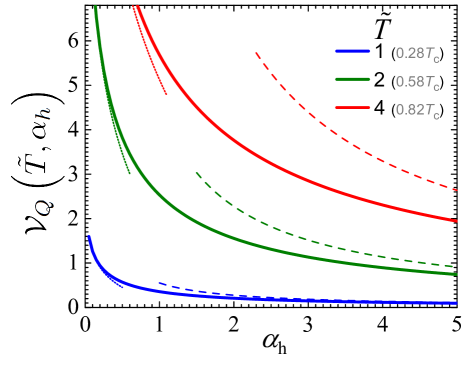
Figure 5: Plots of the function $\mathcal{V}_{Q}(\tilde{T},\alpha_{h})$ in Eq. (57b) which determines the correction to the electromagnetic kernel and London penetration depth in Eq. (57a). The dashed lines show large-$\alpha_{h}$ asymptotics, $\mathcal{V}_{Q}(\tilde{T},\alpha_{h})\propto 1/\alpha_{h}$, corresponding to the scattering regime. The dotted lines show small-$\alpha_{h}$ asymptotics, $\mathcal{V}_{Q}(\tilde{T},\alpha_{h})\propto\ln\left(1/\alpha_{h}\right)$.

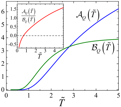
Figure 6: Temperature dependence of the coefficients $\mathcal{A}_{Q}(\tilde{T})$ and $\mathcal{B}_{Q}(\tilde{T})$ defined by Eqs. (58b) and (58c), respectively, which determine the small-$\alpha_{h}$ asymptotics of the function $\mathcal{V}_{Q}(\tilde{T},\alpha_{h})$, Eq. (58a). The inset shows the temperature dependence of their ratio. The coefficient $\mathcal{A}_{Q}(\tilde{T})$ changes sign at $\tilde{T}=0.683$.

Similar to Eq. (40), we can present the correction in Eq. (57a) in the limit $\xi_{h}\gg\xi_{s}$ as

$$\lambda_{1\alpha}^{-2}\!=\!-\!\lambda_{0\alpha}^{-2}\frac{h_{0}^{2}\mathcal{B}_{Q}\!(\tilde{T})}{2\Delta_{0}^{2}}\!\left[1\!-\!\frac{\ln\left(\frac{\xi_{s}}{a}\right)\!-\!\mathcal{A}_{Q}\!(\tilde{T})\!/\!\mathcal{B}_{Q}\!(\tilde{T})}{\ln\left(\xi_{h}/a\right)}\right].$$ (59)

The ratio $\mathcal{A}_{Q}\!(\tilde{T})\!/\!\mathcal{B}_{Q}\!(\tilde{T})$ is of the order unity in the whole temperature range and becomes negative for $\tilde{T}<0.683$, see inset in Fig. 6, meaning that the nominator $\ln\left(\xi_{s}/a\right)\!-\!\mathcal{A}_{Q}\!(\tilde{T})\!/\!\mathcal{B}_{Q}\!(\tilde{T})$ is always positive. As a consequence, the correction to the superfluid density monotonically increases when temperature approaches $T_{m}$. This is different from the behavior of the gap correction, Eq. (36a), which becomes nonmonotonic at small temperatures. The maximum suppression of $\lambda_{\alpha}^{-2}$ for $\xi_{h}\rightarrow\infty$, $\lambda_{1\alpha,\mathrm{max}}^{-2}\!=\!-\lambda_{0\alpha}^{-2}\left(h_{0}^{2}/2\Delta_{0}^{2}\right)\mathcal{B}_{Q}\!\left(2\pi T_{m}/\Delta_{0}\right)$, corresponds to the correction from a uniform exchange field equal to $h_{0}$.

VI Discussion

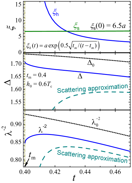
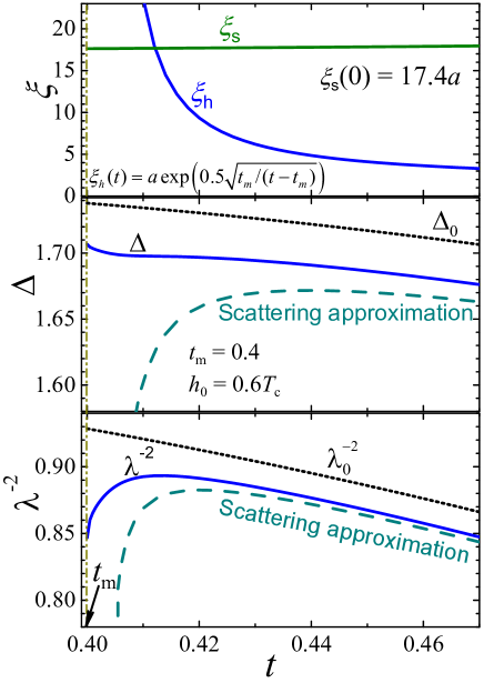
Figure 7: The middle and bottom panels in both plots show computed dependences of the gap $\Delta$ and superfluid density $\propto\lambda^{-2}$ on the reduced temperature $t=T/T_{c}$. The dotted lines show unperturbed values and dashed lines show the results obtained within the scattering approximation. The unit of $\Delta$ is $T_{c}$ and the unit of $\lambda^{-2}$ is $\left[\lambda_{0}(0)\right]^{-2}$. The top panel shows the assumed temperature dependences of the magnetic correlation length and coherence length. The plots on the left side are made for the parameters roughly corresponding to RbEuFe₄As₄ (see text). The plots on the right side are made for the same parameters as in the left plots except for 2.7 times larger coherence length. In this case the scattering-regime asymptotics are much more pronounced and the gap has nonmonotonic temperature dependence.

In summary, we evaluated the corrections to the gap, Eq. (36a), and superfluid density, Eq. (57a), caused by the exchange interaction with quasi-two-dimensional magnetic fluctuations in materials composed of superconducting and local-moment layers. Growth of the correlation length near the magnetic transition enhances spin-flip scattering leading to increasing suppression of superconducting parameters. This suppression significantly weakens when the magnetic correlation length exceeds the coherence length. In addition to dependence on the correlation length $\xi_{h}(T)$, the corrections have also direct regular dependence on the ratio $T/\Delta_{0}(T)$. Moreover, as one can see from Figs. 3 and 5, in the paramagnetic state these dependences are opposite. While in the immediate vicinity of the magnetic transition the growth of $\xi_{h}(T)$ dominates, in a wider range, the overall temperature dependence is determined by the interplay between both sources. To generate the parameter’s temperature dependences for real materials from the derived general formulas, one need to specify the temperature dependent gap, coherence length, and magnetic correlation length, as well as the strength of the exchange field.

Even though the consideration of this paper has been mostly motivated by physics of RbEuFe₄As₄, at present, there are too many uncertainties in the parameters of this material to make a reliable quantitative predictions. Therefore, we limit ourselves with showing expected qualitative behavior using representative parameters and illustrating general trends. Figure 7(left) shows the temperature dependences of the gap and $\lambda^{-2}$ for the parameters very roughly corresponding to RbEuFe₄As₄. Namely, we assume (i)the the Ginzburg-Landau coherence length $\xi_{s0}^{\mathrm{GL}}\!=\!1.46$nm, following from the linear slope of the c-axis upper critical field [21, 22], (ii) the BCS value of the zero-temperature gap, $\Delta_{0}(0)\!=\!1.76T_{c}\!\approx\!5.6$meV, (iii) the BCS temperature dependences for all unperturbed superconducting parameters, (iv) the amplitude of the exchange field $h_{0}\!=\!0.6T_{c}$, (v) the magnetic transition at $t_{m}\!\equiv\!T_{m}/T_{c}\!=\!0.4$, and (vi) Berezinskii-Kosterlitz-Thouless (BKT) shape for the magnetic correlation length, $\xi_{h}(T)\!=\!a\exp[b\sqrt{T_{m}/(T\!-\!T_{m})}]$, where $a\!=\!0.39$ nm is the distance between the neighboring Eu²⁺ moments and we take the value $b\!=\!0.5$ for nonuniversal numerical constant. For these parameters, $\xi_{s}(T_{m})=6.6a$ and the ’scattering-to-smooth’ crossover is nominally located at $t_{\mathrm{cr}}\!\approx\!0.43$. We see, however, that above this temperature the behavior is not well described by the scattering-regime asymptotics shown by the dashed lines. This is related to the broad range of the crossover. Consequently, for selected parameters, the gap does not display a nonmonotonic behavior, expected from the analysis of asymptotics. In fact, due to the interplay between two competing temperature dependences, both corrections are almost temperature independent in the range $0.42<t<0.47$. Nevertheless, we see that, according to the general predictions, $\Delta(T)$ somewhat increases when $T$ approaches $T_{m}$, while $[\lambda(T)]^{-2}$ shows a noticeable drop. For illustrative purposes, we show in Fig. 7(right) the plots of $\Delta(T)$ and $[\lambda(T)]^{-2}$ for the same parameters as in the previous figure except for larger coherence length, $\xi_{s0}^{\mathrm{GL}}\!=\!10a\!\approx\!3.9$nm. In this case $\xi_{s}(T_{m})\!=\!17.6a$ and the crossover nominally takes place much closer to $t_{m}$, at $t_{\mathrm{cr}}\!\approx\!0.41$. In this case the behavior at $t>0.43-0.44$ is already fairly well described by the scattering asymptotics. The gap in this case does have a nonmonotonic temperature dependence.

Clearly, the plots in Fig. 7(left) do not literally describe the behavior of RbEuFe₄As₄ and serve only as a qualitative illustration. This material has several additional features that influence the behavior of the parameters but substantially complicate an accurate analysis. Firstly, the assumed two-dimensional behavior always breaks down sufficiently close to the transition and the dimensional crossover to the three-dimensional regime takes place. In this 3D regime the correlations between the different magnetic layers emerge meaning that the assumption for two-dimensional scattering does not work any more. In addition, the magnetic correlation length does not follow the BKT temperature dependence assumed in Fig. 7. Secondly, due to spatial separation between the magnetic and conducting layers, we expect a significant nonlocality of the exchange interaction, see Eq. (5), ranging at least 2–3 lattice spacing. Consideration of this manuscript assumes that the magnetic correlation length exceeds this nonlocality range. This assumption is only justified close to the magnetic transition. The nonlocality significantly reduces the exchange corrections at higher temperatures, when $\xi_{h}$ drops below the nonlocality range. Finally, our single-band consideration does not take into account a complicated multiple-band structure of RbEuFe₄As₄.

In this paper, we developed a general theoretical framework for the analysis of the influence of correlated magnetic fluctuations on superconducting parameters. We focus on the behavior of the gap and superfluid density for the in-plane current direction, but the consideration can be directly extended to other thermodynamic and transport properties. For some properties, however, such as specific heat and magnetization, a reliable separation of the superconducting contribution from the magnetic background in experiment is challenging. This makes a theoretical analysis somewhat academic. Our result can be straightforwardly generalized to the case of a large exchange field leading to a strong suppression of superconductivity. Such generalization requires the development of a self-consistent scheme similar to the AG theory[1]. For the problem considered here, this is a formidable theoretical task.

Appendix A Calculation of the integral for the gap correction

In this appendix we briefly describe calculation of the integral in Eq. (33) leading to result in Eq. (34). Substituting the function $W(z,g)$ defined in Eq. (26) into Eq. (33), we present $\delta\mathcal{I}$ as

$$\delta\mathcal{I}\!=\!-\frac{C_{h}\nu h_{0}^{2}}{4\pi}\frac{\Delta_{0}}{\left(\omega_{n}^{2}\!+\!\Delta_{0}^{2}\right)^{3/2}}\left[\mathcal{T}_{1}(g_{n})\!+\!\frac{4\omega_{n}^{2}}{\omega_{n}^{2}\!+\!\Delta_{0}^{2}}\mathcal{T}_{2}(g_{n})\right],$$ (60)

where

$$\mathcal{T}_{1}(g) =\mathrm{Re}\left[\int\limits_{-\infty}^{\infty}dz\frac{2}{\left(z+i\right)^{2}\sqrt{\left(iz+1\right)^{2}-g^{2}}}\right.$$

$$\times \left.\ln\left(\frac{iz+1+\sqrt{\left(iz+1\right)^{2}-g^{2}}}{g}\right)\right],$$

$$\mathcal{T}_{2}(g) =\mathrm{Re}\left[\int\limits_{-\infty}^{\infty}dz\frac{2}{\left(z^{2}+1\right)^{2}\sqrt{\left(iz+1\right)^{2}-g^{2}}}\right.$$

$$\times \left.\ln\left(\frac{iz+1+\sqrt{\left(iz+1\right)^{2}-g^{2}}}{g}\right)\right].$$

The integral for $\mathcal{T}_{1}(g)$ has a pole at $z=-i$ and branches at the imaginary axis terminating at $z_{\pm}=i\left(1\pm g\right)$. Deforming the integration contour into the complex plane, we reduce it to the integral along the square-root branch $z=ix$, $1+g<x<\infty$ ,

$$\mathcal{T}_{1}(g) =-2\pi\int\limits_{1+g}^{\infty}dx\frac{2}{\left(x+1\right)^{2}\sqrt{\left(x-1\right)^{2}-g^{2}}}$$

$$=4\pi\left[\frac{1}{4-g^{2}}-\frac{2}{\left(4-g^{2}\right)^{3/2}}\ln\left(\frac{2+\sqrt{4-g^{2}}}{g}\right)\right].$$

The integral for $\mathcal{T}_{1}(g)$ has the same square-root branches and the poles at $z=\pm i$. Consequently, we split the integral into contribution from the pole at $z=i$ and square-root branch $z=ix$, $1+g<x<\infty$ which yields

$$\mathcal{T}_{2}(g) =\frac{\pi^{2}}{2g}-\frac{\pi}{g^{2}}+4\pi\int\limits_{1+g}^{\infty}dx\frac{1}{\left(x^{2}-1\right)^{2}\sqrt{\left(x-1\right)^{2}-g^{2}}}$$

$$=-\pi\left[\frac{1}{4-g^{2}}-\frac{6-g^{2}}{\left(4-g^{2}\right)^{3/2}}\ln\left(\frac{2+\sqrt{4-g^{2}}}{g}\right)\right]$$

Substituting the above results into Eq. (60), we arrive to Eq. (34).

Appendix B Magnetic-scattering correction to the London penetration depth using quasiclassical approach

The London penetration depth $\lambda$ in the presence of isotropic potential and magnetic scattering has been investigated within the quasiclassical approach in Ref. [30]. Here we derive a general equation for $\lambda$ for arbitrary magnetic scattering having in mind application to the case of correlated magnetic fluctuations. The Eilenberger equations for the quasiclassical Green’s functions, $f(\boldsymbol{p},\boldsymbol{r})$, $f^{\dagger}(\boldsymbol{p},\boldsymbol{r})$, and $g(\boldsymbol{p},\boldsymbol{r})$ for arbitrary scattering are [32]

$$\bm{v}\bm{\Pi}f=2\Delta g-2\omega_{n}f$$

$$+g\left\langle\left[W(\boldsymbol{p},\boldsymbol{p}^{\prime})\!-W_{m}(\boldsymbol{p},\boldsymbol{p}^{\prime})\right]f{}^{\prime}\right\rangle^{\prime}\!$$

$$-\!f\left\langle\left[W(\boldsymbol{p},\boldsymbol{p}^{\prime})\!+\!W_{m}(\boldsymbol{p},\boldsymbol{p}^{\prime})\right]g{}^{\prime}\right\rangle^{\prime},$$ (61a)

$$-\! \!\bm{v}\bm{\Pi}^{*}\!f^{\dagger}\!=\!2\Delta^{*}g\!-\!2\omega_{n}f^{\dagger}\!$$

$$+\!g\left\langle\left[W(\boldsymbol{p},\boldsymbol{p}^{\prime})\!-\!W_{m}(\boldsymbol{p},\boldsymbol{p}^{\prime})\right]f^{\dagger}{}^{\prime}\right\rangle^{\prime}\!$$

$$-\!f^{\dagger}\left\langle\left[W(\boldsymbol{p},\boldsymbol{p}^{\prime})\!+\!W_{m}(\boldsymbol{p},\boldsymbol{p}^{\prime})\right]g{}^{\prime}\right\rangle^{\prime}\!,$$ (61b)

where we used shortened notations $f\!\equiv\!f(\boldsymbol{p},\boldsymbol{r})$, $f^{\prime}\!\equiv\!f(\boldsymbol{p}^{\prime},\boldsymbol{r})$, $\bm{\Pi}f\!\equiv\!\left(\boldsymbol{\nabla}\!+\!2\pi i\bm{\bm{A}}/\phi_{0}\right)f$, $\left\langle A(\boldsymbol{p}^{\prime})\right\rangle^{\prime}\!\equiv\!\int_{S_{F}}\!d^{2}\boldsymbol{p}^{\prime}\rho(\boldsymbol{p}^{\prime})A(\boldsymbol{p}^{\prime})$, and $\rho(\boldsymbol{p})\!=\!\left[(2\pi)^{3}\nu v_{F}(\boldsymbol{p})\right]^{-1}$. Further, $W(\boldsymbol{p},\boldsymbol{p}^{\prime})$ and $W_{m}(\boldsymbol{p},\boldsymbol{p}^{\prime})$ are the probabilities of potential and magnetic scattering defining the corresponding scattering times as

$$\frac{1}{\tau}=\left\langle W(\boldsymbol{p},\boldsymbol{p}^{\prime})\right\rangle^{\prime},\,\frac{1}{\tau_{m}}=\left\langle W_{m}(\boldsymbol{p},\boldsymbol{p}^{\prime})\right\rangle^{\prime}.$$

For the model considered in this paper $W_{m}(\boldsymbol{p},\boldsymbol{p}^{\prime})=2\pi\nu\left\langle\left|\tilde{\boldsymbol{h}}_{\boldsymbol{p}-\boldsymbol{p}^{\prime}}\right|^{2}\right\rangle$ . The above equations have to be supplemented with the normalization condition $g^{2}=1-ff^{\dagger}$, the gap equation

$$\frac{\Delta}{2\pi T}\ln\frac{T_{c0}}{T}=\sum_{\omega_{n}>0}\left(\frac{\Delta}{\omega}-\langle f\rangle\right),$$ (62)

and formula for the current

$$\bm{j}=4\pi e\nu T\,{\rm Im}\sum_{\omega_{n}>0}\langle\bm{v}g\rangle.$$ (63)

Our goal is to derive the response to weak supercurrents. In linear order, weak supercurrents do not modify the gap absolute value but only add the same phase $\theta(\bm{r})$ to $\Delta$ and $f$ and the opposite phase to $f^{\dagger}$. Therefore, the linear-order solutions have the form,

$$\Delta=\Delta_{0}\,e^{i\theta},\,f=(f_{0}+f_{1})\,e^{i\theta},$$

$$f^{\dagger}=(f_{0}+f_{1})e^{-i\theta},\,g=g_{0}+g_{1}\,,$$

where only the phase $\theta$ has coordinate dependence, while $f_{1},f_{1}^{\dagger},g_{1}$ are uniform meaning that $\bm{\Pi}f=i\bm{P}f$ and $\bm{\Pi}^{*}f^{\dagger}=-i\bm{P}f^{\dagger}$ with $\bm{P}=\nabla\theta+2\pi\bm{\bm{A}}/\phi_{0}$. Equations for the linear corrections are

$$2\Delta_{0} g_{1}\!-\!2\omega_{n}f_{1}\!+\!\frac{g_{1}(\boldsymbol{p})}{\tau_{-}}f_{0}-\frac{f_{1}(\boldsymbol{p})}{\tau_{+}}g_{0}$$

$$+ g_{0}\left\langle\left[W(\boldsymbol{p},\boldsymbol{p}^{\prime})\!-\!W_{m}(\boldsymbol{p},\boldsymbol{p}^{\prime})\right]f_{1}(\boldsymbol{p}^{\prime})\right\rangle^{\prime}\!$$

$$- f_{0}\left\langle\left[W(\boldsymbol{p},\boldsymbol{p}^{\prime})\!+\!W_{m}(\boldsymbol{p},\boldsymbol{p}^{\prime})\right]g_{1}(\boldsymbol{p}^{\prime})\right\rangle^{\prime}\!=\!iv_{\alpha}P_{\alpha}f_{0},$$ (64)

$$g_{0}g_{1}=-f_{0}f_{1}$$ (65)

with $\frac{1}{\tau_{\pm}}=\frac{1}{\tau}\pm\frac{1}{\tau_{m}}.$ The remaining averages in the first equation account for the reverse scattering events. These averages vanish for the case of isotropic scattering. We assume that the solutions are proportional to $v_{\alpha}P_{\alpha}$ and define the corresponding averages as

$$\left\langle W(\boldsymbol{p},\boldsymbol{p}^{\prime})v_{\alpha}^{\prime}\right\rangle^{\prime}=\frac{1}{\tau^{\alpha}}v_{\alpha},\,\left\langle W_{m}(\boldsymbol{p},\boldsymbol{p}^{\prime})v_{\alpha}^{\prime}\right\rangle^{\prime}=\frac{1}{\tau_{m}^{\alpha}}v_{\alpha},$$

giving

$$\frac{1}{\tau^{\alpha}}=\frac{\left\langle\left\langle W(\boldsymbol{p},\boldsymbol{p}^{\prime})v_{\alpha}v_{\alpha}^{\prime}\right\rangle\right\rangle^{\prime}}{\left\langle v_{\alpha}^{2}\right\rangle},\,\frac{1}{\tau_{m}^{\alpha}}=\frac{\left\langle\left\langle W_{m}(\boldsymbol{p},\boldsymbol{p}^{\prime})v_{\alpha}v_{\alpha}^{\prime}\right\rangle\right\rangle^{\prime}}{\left\langle v_{\alpha}^{2}\right\rangle}.$$ (66)

These quantities determine the corresponding transport times in a standard way, $1/\tau^{\mathrm{tr}}=1/\tau-1/\tau^{\alpha}$ and $1/\tau_{m}^{\mathrm{tr}}=1/\tau_{m}-1/\tau_{m}^{\alpha}$. In the case of correlated magnetic fluctuation which we consider in this paper, the transport rate is much smaller than the total scattering rate. The averagings in Eq. (64) can now be performed as,

$$\left\langle\left[W(\boldsymbol{p},\boldsymbol{p}^{\prime})\!\pm W_{m}(\boldsymbol{p},\boldsymbol{p}^{\prime})\right]f_{1}(\boldsymbol{p}^{\prime})\right\rangle^{\prime}\!=\frac{f_{1}(\boldsymbol{p})}{\tau_{\pm}^{\alpha}}.$$

with $1/\tau_{\pm}^{\alpha}=1/\tau^{\alpha}\pm 1/\tau_{m}^{\alpha}$. This allows us to rewrite Eq. (64) as

$$2\Delta_{0}g_{1}\!-\!2\omega_{n}f_{1}\!+\frac{g_{1}}{\tau_{-}}f_{0}\!+g_{0}\frac{f_{1}}{\tau_{-}^{\alpha}}\!-\frac{f_{1}}{\tau_{+}}g_{0}-f_{0}\frac{g_{1}}{\tau_{+}^{\alpha}}=iv_{\alpha}P_{\alpha}f_{0},$$ (67)

Substituting $g_{1}=-f_{0}f_{1}/g_{0}$ from Eq. (65), we obtain the solutions

$$f_{1} =-\frac{\!iv_{\alpha}f_{0}P_{\alpha}}{2\omega_{n}\!+\!2\Delta_{0}\frac{f_{0}}{g_{0}}\!+\!\frac{f_{0}^{2}}{g_{0}}\left(\frac{1}{\tau_{-}}\!-\!\frac{1}{\tau_{+}^{\alpha}}\right)\!+\!g_{0}\left(\frac{1}{\tau_{+}}\!-\!\frac{1}{\tau_{-}^{\alpha}}\right)},$$ (68)

$$g_{1} =\frac{f_{0}^{2}}{g_{0}}\frac{\!iv_{\alpha}P_{\alpha}}{2\omega_{n}\!+\!2\Delta_{0}\frac{f_{0}}{g_{0}}\!+\!\frac{f_{0}^{2}}{g_{0}}\left(\frac{1}{\tau_{-}}\!-\!\frac{1}{\tau_{+}^{\alpha}}\right)\!+\!g_{0}\left(\frac{1}{\tau_{+}}\!-\!\frac{1}{\tau_{-}^{\alpha}}\right)}.$$ (69)

We can rewrite the scattering-rate differences here in terms of scattering and transport times as

$$\frac{1}{\tau_{-}}\!-\!\frac{1}{\tau_{+}^{\alpha}} =\frac{1}{\tau^{\mathrm{tr}}}-\frac{2}{\tau_{m}}+\frac{1}{\tau_{m}^{\mathrm{tr}}},$$

$$\frac{1}{\tau_{+}}\!-\!\frac{1}{\tau_{-}^{\alpha}} =\frac{1}{\tau^{\mathrm{tr}}}+\frac{2}{\tau_{m}}-\frac{1}{\tau_{m}^{\mathrm{tr}}}.$$

We use a standard parametrization for the unperturbed Green’s function components

$$f_{0}=\frac{1}{\sqrt{1+u^{2}}},\>g_{0}=\frac{u}{\sqrt{1+u^{2}}}.$$

The parameter $u$ obeys the Abrikosov-Gor’kov equation[1, 3]

$$u\left(1-\frac{1}{\tau_{m}\Delta\sqrt{1+u^{2}}}\right)=\frac{\omega_{n}}{\Delta}.$$ (70)

and determines the gap via equation

$$\Delta\ln\frac{T_{c0}}{T}=2\pi T\sum_{\omega_{n}>0}\left(\frac{\Delta}{\omega_{n}}-\frac{1}{\sqrt{1+u^{2}}}\right).$$ (71)

We proceed with the derivation of the current response using Eq. (63). Rewriting $g_{1}$ in Eq. (69) in terms of the parameter $u$

$$g_{1}=\frac{\!iv_{\alpha}P_{\alpha}}{\left(1+u^{2}\right)\left(2\Delta\sqrt{1+u^{2}}+\!\frac{1}{\tau_{-}^{\mathrm{tr}}}\right)\!-\!\frac{2}{\tau_{m}^{\alpha}}}.$$

and substituting it into Eq. (63), we obtain the linear current response as

$$j_{\alpha}\!=\!4\pi e\nu T\sum_{\omega_{n}>0}\frac{\langle v_{\alpha}^{2}\rangle}{\left(1\!+\!u^{2}\right)\left(2\Delta\sqrt{1\!+\!u^{2}}+\!\frac{1}{\tau_{-}^{\mathrm{tr}}}\right)\!-\!\frac{2}{\tau_{m}^{\alpha}}}P_{\alpha}.$$ (72)

Using the definition $4\pi j_{\alpha}/c=-\lambda_{\alpha}^{-2}A_{\alpha}$ and $P_{\alpha}=2\pi\,A_{\alpha}/\phi_{0}$, we finally obtain the result for $\lambda_{\alpha}^{-2}$,

$$\lambda_{\alpha}^{-2}\!=\!\frac{16\pi^{3}|e|\nu\langle v_{\alpha}^{2}\rangle}{c\phi_{0}}T\!\!\sum_{\omega_{n}\!>0}\frac{1}{\left(1\!+\!u^{2}\right)\left(\Delta\sqrt{1\!+\!u^{2}}+\!\frac{1}{2\tau_{-}^{\mathrm{tr}}}\right)\!-\!\frac{1}{\tau_{m}^{\alpha}}}.$$ (73)

This result can be used for self-consistent evaluation of the London penetration depth of arbitrary scattering. Note that it is different from the similar result in Ref. [2] by the sign in front of $\frac{1}{\tau_{m}^{\alpha}}$ in the denominator.

B.0.1 Small-scattering-rate expansion

For comparison with the results in the main text, we derive small correction to $\lambda_{\alpha}^{-2}$ in the case of weak scattering. Expanding the parameter $u$ in Eq. (70), $u=\frac{\omega_{n}}{\Delta}+u_{m},$ we obtain

$$u_{m}\approx\frac{\omega_{n}}{\tau_{m}\Delta\sqrt{\omega_{n}^{2}+\Delta^{2}}}.$$

Substituting this expansion into the gap equation, Eq. (71), we derive the correction to the gap, $\Delta=\Delta_{0}+\tilde{\Delta}$,

$$\tilde{\Delta} \!=\!-\frac{2\pi T}{\tau_{m}\Delta_{0}}\!\sum_{\omega_{n}>0}\frac{\omega_{n}^{2}}{\left(\Delta_{0}^{2}\!+\!\omega_{n}^{2}\right)^{2}}\left[2\pi T\!\!\sum_{\omega_{n}>0}\frac{1}{\left(\Delta_{0}^{2}\!+\!\omega^{2}\right)^{3/2}}\right]^{-1}\!.$$ (74)

In the reduced form, this correction is identical to Eq. (38).

To derive the correction to $\lambda_{\alpha}^{-2}$, we expand the fraction in Eq. (73)

$$\frac{1}{\left(1\!+\!u^{2}\right)\left(\Delta\sqrt{1\!+\!u^{2}}\!+\!\frac{1}{2\tau_{-}^{\mathrm{tr}}}\right)\!-\!\frac{1}{\tau_{m}^{\alpha}}}\!\approx\!\frac{\Delta^{2}}{\left(\Delta^{2}\!+\!\omega_{n}^{2}\right)^{3/2}}$$

$$\times\left(\!1\!-\frac{3\omega_{n}^{2}-\Delta^{2}}{\tau_{m}\left(\Delta^{2}\!+\!\omega_{n}^{2}\right)^{3/2}}\!+\frac{\omega_{n}^{2}-\Delta^{2}}{2\tau_{m}^{\mathrm{tr}}\left(\Delta^{2}\!+\!\omega_{n}^{2}\right)^{3/2}}\!\right.$$

$$-\left.\frac{1}{2\tau^{\mathrm{tr}}\sqrt{\Delta^{2}\!+\!\omega_{n}^{2}}}\!\right)$$

and also separate the contribution from the gap correction

$$\frac{\Delta^{2}}{\left(\Delta^{2}\!+\!\omega_{n}^{2}\right)^{3/2}} \approx\frac{\Delta_{0}^{2}}{\left(\Delta_{0}^{2}+\omega_{n}^{2}\right)^{3/2}}+\frac{\Delta_{0}\tilde{\Delta}\left(2\omega_{n}^{2}\!-\!\Delta_{0}^{2}\right)}{\left(\Delta_{0}^{2}+\omega_{n}^{2}\right)^{5/2}}.$$

This gives the correction to $\lambda_{\alpha}^{-2}$,

$$\lambda_{\alpha}^{-2} \approx\lambda_{0\alpha}^{-2}+\lambda_{1\alpha}^{-2},$$

$$\lambda_{0\alpha}^{-2} =\!\frac{16\pi^{4}\nu\langle v_{\alpha}^{2}\rangle}{\phi_{0}^{2}}T\sum_{\omega_{n}>0}\frac{\Delta_{0}^{2}}{\left(\Delta_{0}^{2}+\omega_{n}^{2}\right)^{3/2}},$$

$$\lambda_{1\alpha}^{-2} =\!\frac{16\pi^{4}\nu\langle v_{\alpha}^{2}\rangle}{\phi_{0}^{2}}T\!\sum_{\omega_{n}>0}\!\left[\frac{\Delta_{0}\tilde{\Delta}\left(2\omega_{n}^{2}\!-\!\Delta_{0}^{2}\right)}{\left(\Delta_{0}^{2}+\omega_{n}^{2}\right)^{5/2}}\right.$$

$$- \frac{\Delta_{0}^{2}\left(3\omega_{n}^{2}\!-\!\Delta_{0}^{2}\right)}{\tau_{m}\left(\Delta_{0}^{2}+\omega_{n}^{2}\right)^{3}}+\frac{\Delta_{0}^{2}\left(\omega_{n}^{2}\!-\!\Delta_{0}^{2}\right)}{2\tau_{m}^{\mathrm{tr}}\left(\Delta_{0}^{2}\!+\!\omega_{n}^{2}\right)^{3}}$$

$$- \left.\frac{\Delta_{0}^{2}}{2\tau^{\mathrm{tr}}\left(\Delta_{0}^{2}\!+\!\omega_{n}^{2}\right)^{2}}\right].$$ (75)

We see that, in contrast to the potential scattering, which only influences the London penetration depth via the transport time, the magnetic-scattering contribution to $\lambda_{1\alpha}^{-2}$ also has contributions proportional to the total scattering rate $1/\tau_{m}$, both direct and via the gap correction. This pair-breaking contribution, however, vanishes at zero temperature. For numerical convenience, we can rewrite the correction in the following reduced form

$$\lambda_{1\alpha}^{-2}(T)=-\lambda_{0\alpha}^{-2}(T)\left[\frac{1}{\tau_{m}\Delta_{0}}V_{\lambda,m}\!\left(\frac{2\pi T}{\Delta_{0}}\right)\right.$$

$$+\left.\frac{1}{\tau_{m}^{\mathrm{tr}}\Delta_{0}}V_{\lambda,m}^{\mathrm{tr}}\!\left(\frac{2\pi T}{\Delta_{0}}\right)\!+\!\frac{1}{\tau^{\mathrm{tr}}\Delta_{0}}V_{\lambda}^{\mathrm{tr}}\!\left(\frac{2\pi T}{\Delta_{0}}\right)\right],$$ (76)

with

$$V_{\lambda,m}(\tilde{T}) \!=\!\left[\mathcal{D}\!(\tilde{T})\right]^{-1}\!\tilde{T}\sum_{n=0}^{\infty}\!\left[\frac{2\tilde{\omega}_{n}^{2}\!-1}{\left(1\!+\!\tilde{\omega}_{n}^{2}\right)^{5/2}}V_{\Delta}(\tilde{T})\!+\!\frac{3\tilde{\omega}_{n}^{2}\!-1}{\left(1\!+\!\tilde{\omega}_{n}^{2}\right)^{3}}\right]\!,$$

$$V_{\lambda,m}^{\mathrm{tr}}(\tilde{T}) \!=\!\frac{1}{2}\left[\mathcal{D}(\tilde{T})\right]^{-1}\!\tilde{T}\sum_{n=0}^{\infty}\frac{1-\tilde{\omega}_{n}^{2}}{\left(1+\tilde{\omega}_{n}^{2}\right)^{3}},$$

$$V_{\lambda}^{\mathrm{tr}}(\tilde{T}) \!=\!\frac{1}{2}\left[\mathcal{D}(\tilde{T})\right]^{-1}\!\tilde{T}\sum_{n=0}^{\infty}\frac{1}{\left(1+\tilde{\omega}_{n}^{2}\right)^{2}},$$

where $\tilde{\omega}_{n}\!\equiv\!\tilde{T}(n\!+\tfrac{1}{2})$, $\mathcal{D}(\tilde{T})$ is defined in Eq. (36c), and $V_{\Delta}(\tilde{T})$ in the formula for $V_{\lambda,m}(\tilde{T})$ is defined in Eq. (37b). For zero temperature, we derive the following result for the gap correction

$$\lambda_{1\alpha}^{-2}(0) =-\frac{\pi}{8}\lambda_{0\alpha}^{-2}\left(\frac{1}{2\tau_{m}^{\mathrm{tr}}\Delta_{0}}+\frac{1}{\tau^{\mathrm{tr}}\Delta_{0}}\right)$$ (77)

with $\lambda_{0\alpha}^{-2}=8\pi^{3}\nu\langle v_{\alpha}^{2}\rangle/\phi_{0}^{2}$. Therefore, the correction to the London penetration depth at $T=0$ in the clean case is proportional to transport scattering rates for both scattering channels.

References

Abrikosov and Gor’kov [1961]A. A. Abrikosov and L. P. Gor’kov, Contribution to the
theory of superconducting alloys with paramagnetic impurities, [Zh. Eksp. Teor. Fiz.
39, 1781 (1960)] Sov. Phys. JETP 12, 1243 (1961).
Skalski et al. [1964]S. Skalski, O. Betbeder-Matibet, and P. R. Weiss, Properties of
superconducting alloys containing paramagnetic impurities, Phys. Rev. 136, A1500 (1964).
Maki [1969]K. Maki, Gapless
Superconductivity, in Superconductivity, Vol. 2, edited by R. D. Parks (Marcel Dekker, New York, 1969) pp. 1035–1105.
Schlottmann [1975]P. Schlottmann, On properties of
superconducting alloys containing Kondo impurities, J. Low Temp. Phys. 20, 123 (1975).
Bulaevskii et al. [1985]L. Bulaevskii, A. Buzdin,
M. Kulić, and S. Panjukov, Coexistence of superconductivity and magnetism
theoretical predictions and experimental results, Adv. Phys. 34, 175 (1985).
Wolowiec et al. [2015]C. T. Wolowiec, B. D. White, and M. B. Maple, Conventional magnetic
superconductors, Physica C 514, 113 (2015).
Kulić and Buzdin [2008]M. Kulić and A. I. Buzdin, Coexistence of Singlet
Superconductivity and Magnetic Order in Bulk Magnetic Superconductors and SF
Heterostructures, in Superconductivity, edited by K. H. Bennemann and J. B. Ketterson (Springer, Berlin, 2008) p. 163.
Maple and Fischer [1982]M. B. Maple and Ø. Fischer, eds., Superconductivity in Ternary
Compounds II, Superconductivity and Magnetism (Springer-Verlag, Berlin, Heidelberg, New York, 1982).
Müller and Narozhnyi [2001]K.-H. Müller and V. N. Narozhnyi, Interaction of
superconductivity and magnetism in borocarbide superconductors, Rep. Prog. Phys. 64, 943 (2001).
Gupta [2006]L. C. Gupta, Superconductivity and
magnetism and their interplay in quaternary borocarbides RNi2B2C, Adv. Phys. 55, 691 (2006).
Mazumdar and Nagarajan [2015]C. Mazumdar and R. Nagarajan, Quaternary
borocarbides: Relatively high Tc intermetallic superconductors and
magnetic superconductors, Physica C 514, 173 (2015).
Zapf and Dressel [2017]S. Zapf and M. Dressel, Europium-based iron pnictides: a
unique laboratory for magnetism, superconductivity and structural effects, Rep. Prog. Phys. 80, 016501 (2017).
Liu et al. [2016a]Y. Liu, Y.-B. Liu,
Z.-T. Tang, H. Jiang, Z.-C. Wang, A. Ablimit, W.-H. Jiao, Q. Tao, C.-M. Feng, Z.-A. Xu, and G.-H. Cao, Superconductivity and ferromagnetism
in hole-doped , Phys. Rev. B 93, 214503 (2016a).
Liu et al. [2016b]Y. Liu, Y.-B. Liu,
Q. Chen, Z.-T. Tang, W.-H. Jiao, Q. Tao, Z.-A. Xu, and G.-H. Cao, A new
ferromagnetic superconductor:
, Science Bulletin 61, 1213 (2016b).
Kawashima et al. [2016]K. Kawashima, T. Kinjo,
T. Nishio, S. Ishida, H. Fujihisa, Y. Gotoh, K. Kihou, H. Eisaki, Y. Yoshida, and A. Iyo, Superconductivity in Fe-based compound EuAFe4As4 (A = Rb and
Cs), J. Phys. Soc. Jpn. 85, 064710 (2016).
Bao et al. [2018]J.-K. Bao, K. Willa, M. P. Smylie, H. Chen, U. Welp, D. Y. Chung, and M. G. Kanatzidis, Single
crystal growth and study of the ferromagnetic superconductor
RbEuFe4As4, Crystal Growth & Design 18, 3517 (2018).
Rainer [1972]D. Rainer, Influence of correlated
spins on the superconducting transition temperature, Z. Phys. 252, 174 (1972).
Machida and Youngner [1979]K. Machida and D. Youngner, Superconductivity of
ternary rare-earth compounds, J. Low Temp. Phys. 35, 449 (1979).
Bud’ko and Canfield [2000]S. L. Bud’ko and P. C. Canfield, Rotational tuning of
anomalies in :
Angular-dependent superzone gap formation and its effect on the
superconducting ground state, Phys. Rev. B 61, R14932 (2000).
Smylie et al. [2018]M. P. Smylie, K. Willa,
J.-K. Bao, K. Ryan, Z. Islam, H. Claus, Y. Simsek, Z. Diao, A. Rydh, A. E. Koshelev,
W.-K. Kwok, D. Y. Chung, M. G. Kanatzidis, and U. Welp, Anisotropic superconductivity and magnetism in single-crystal
, Phys. Rev. B 98, 104503 (2018).
Willa et al. [2019]K. Willa, R. Willa,
J.-K. Bao, A. E. Koshelev, D. Y. Chung, M. G. Kanatzidis, W.-K. Kwok, and U. Welp, Strongly fluctuating moments in the high-temperature magnetic
superconductor , Phys. Rev. B 99, 180502(R) (2019).
Iida et al. [2019]K. Iida, Y. Nagai,
S. Ishida, M. Ishikado, N. Murai, A. D. Christianson, H. Yoshida, Y. Inamura, H. Nakamura, A. Nakao, K. Munakata, D. Kagerbauer, M. Eisterer, K. Kawashima, Y. Yoshida, H. Eisaki, and A. Iyo, Coexisting
spin resonance and long-range magnetic order of Eu in
, Phys. Rev. B 100, 014506 (2019).
Islam et al. [2020]Z. Islam, O. Chmaissem,
A. E. Koshelev, J.-W. Kim, H. Cao, A. Rydh, M. P. Smylie, K. Willa, J. Bao, D. Y. Chung, M. Kanatzidis, W.-K. Kwok, S. Rosenkranz, and U. Welp, unpublished (2020).
Collomb et al. [2020]D. Collomb, S. Bending,
A. E. Koshelev, M. P. Smylie, L. Farrar, J. Bao, D. Y. Chung, M. Kanatzidis, W.-K. Kwok, and U. Welp, unpublished (2020).
Coffey et al. [1983]L. Coffey, K. Levin, and G. S. Grest, Theory of superconductivity in reentrant
superconductors: Tunneling in paramagnetic phase, Phys. Rev. B 27, 2740 (1983).
Schossmann and Carbotte [1987]M. Schossmann and J. P. Carbotte, On dynamical effects in
reentrant magnetic superconductors, J. Low Temp. Phys. 69, 349 (1987).
Gor’kov et al. [1965]L. P. Gor’kov, A. A. Abrikosov, and I. E. Dzyaloshinskii, Quantum Field
Theoretical Methods in Statistical Physics (Pergamon Press Oxford, 1965).
Kopnin [2001]N. Kopnin, Theory of nonequilibrium
superconductivity, Vol. 110 (Oxford University Press, Oxford, 2001).
Kogan et al. [2013]V. G. Kogan, R. Prozorov, and V. Mishra, London penetration depth and pair
breaking, Phys. Rev. B 88, 224508 (2013).
Maekawa et al. [1979]S. Maekawa, M. Tachiki, and S. Takahashi, Vortex structure in ferromagnetic
superconductors, J. Magn. Magn. Mater. 13, 324 (1979).
Eilenberger [1968]G. Eilenberger, Transformation of
Gorkov’s equation for type II superconductors into transport-like
equations, Z. Phys. A 214, 195 (1968).