QEBA: Query-Efficient Boundary-Based Blackbox Attack

Abstract

Machine learning (ML), especially deep neural networks (DNNs) have been widely used in various applications, including several safety-critical ones (e.g. autonomous driving). As a result, recent research about adversarial examples has raised great concerns. Such adversarial attacks can be achieved by adding a small magnitude of perturbation to the input to mislead model prediction. While several whitebox attacks have demonstrated their effectiveness, which assume that the attackers have full access to the machine learning models; blackbox attacks are more realistic in practice. In this paper, we propose a Query-Efficient Boundary-based blackbox Attack (QEBA) based only on model’s final prediction labels. We theoretically show why previous boundary-based attack with gradient estimation on the whole gradient space is not efficient in terms of query numbers, and provide optimality analysis for our dimension reduction-based gradient estimation. On the other hand, we conducted extensive experiments on ImageNet and CelebA datasets to evaluate QEBA. We show that compared with the state-of-the-art blackbox attacks, QEBA is able to use a smaller number of queries to achieve a lower magnitude of perturbation with 100% attack success rate. We also show case studies of attacks on real-world APIs including MEGVII Face++ and Microsoft Azure.

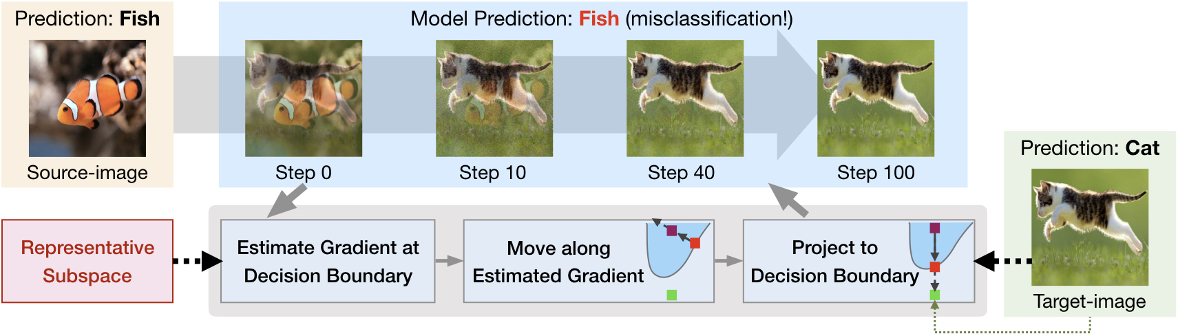
Figure 1: Pipeline of QEBA. In this example, the attack goal is to obtain an adv-image that looks like a cat (target-image) but be misclassified as a fish ($y_{mal}$). We start from a source-image together with an optimized subspace. We then iterativelly perform gradient estimation with queries, move along the estimated direction, and project the new instance to the decision boundary by binary search towards the target-image till converge. The grey solid arrows indicate steps within each iteration. In particular, we show a toy example of how the source-image (purple rectangles) is moved towards the target-image (green rectangles), while the intermediate projected boundary-image is shown as red rectangles.

1 Introduction

Recent developments of machine learning (ML), especially deep neural networks (DNNs), have advanced a number of real-world applications, including object detection [30], drug discovery [8], and robotics [22]. In the meantime, several safety-critical applications have also adopted ML, such as autonomous driving vehicles [7] and surgical robots [31, 32]. However, recent research have shown that machine learning systems are vulnerable to adversarial examples, which are inputs with small magnitude of adversarial perturbations added and therefore cause arbitrarily incorrect predictions during test time [13, 40, 4, 14, 5, 6]. Such adversarial attacks have led to great concerns when applying ML to real-world applications. Thus in-depth analysis of the intrinsic properties of these adversarial attacks as well as potential defense strategies are required.

First, such attacks can be categorized into whitebox and blackbox attacks based on the attacker’s knowledge about the victim ML model. In general, the whitebox attacks are possible by leveraging the gradient of the model — methods like fast gradient sign method (FGSM)  [14], optimization based attack [4], projected gradient descent based method (PGD) [25] have been proposed. However, whitebox attack is less practical, given the fact that most real-world applications will not release the actual model they are using. In addition, these whitebox attacks are shown to be defendable [25]. As a result, blackbox adversarial attack have caught a lot of attention in these days. In blackbox attack, based on whether an attacker needs to query the victim ML model, there are query-free (e.g. transferability based attack) and query-based attacks. Though transferability based attack does not require query access to the model, it assumes the attacker has access to the large training data to train a substitute model, and there is no guarantee for the attack success rate. The query based attack includes score-based and boundary-based attacks. Score-based attack assumes the attacker has access to the class probabilities of the model, which is less practical compared with boundary-based attack which only requires the final model prediction, while both require large number of queries.

In this paper, we propose Query-Efficient Boundary-based blackbox Attack (QEBA) based only on model’s final prediction labels as a general framework to minimize the query number. Since the gradient estimation consumes the majority of all the queries, the main challenge of reducing the number of queries for boundary-based blackbox attack is that a high-dimensional data (e.g. an image) would require large number of queries to probe the decision boundary. As a result, we propose to search for a small representative subspace for query generation. In particular, queries are generated by adding perturbations to an image. We explore the subspace optimization methods from three novel perspectives for perturbation sampling: 1) spatial, 2) frequency, and 3) intrinsic component. The first one leverages spatial transformation (e.g. linear interpolation) so that the sampling procedure can take place in a low-dimensional space and then project back to the original space. The second one uses intuition from image compression literature and samples from low frequency subspace and use discrete consine transformation (DCT) [15] to project back. The final one performs scalable gradient matrix decomposition to select the major principle components via principle component analysis (PCA) [39] as subspace to sample from. In addition , we theoretically prove the optimality of them on estimating the gradient compared with estimating the gradient directly over the original space.

To demonstrate the effectiveness of the proposed blackbox attack QEBA methods, we conduct extensive experiments on high dimensional image data including ImageNet [11] and CelebA [24]. We perform attacks on the ResNet model [17], and show that compared with the-state-of-the-art blackbox attack methods, the different variations of QEBA can achieve lower magnitude of perturbation with smaller number of queries (attack success rate 100%). In order to show the real-world impact of the proposed attacks, we also perform QEBA against online commercial APIs including MEGVII Face++[26] and Microsoft Azure[28]. Our methods can successfully attack the APIs with perturbations of reasonable magnitude. Towards these different subspaces, our conjecture is that the over-all performance on different subspaces depends on multiple factors including dataset size, model smoothness, adversarial attack goals etc. Therefore, our goal here is to make the first attempt towards providing sufficient empirical observations for these three subspaces, while further extensive studies are required to compare different factors of these subspaces, as well as identifying new types of subspaces.

The contributions of this work are summarized as follows: 1) We propose a general Query-Efficient Boundary-based blackbox Attack QEBA to reduce the number of queries based on boundary-based attack. The QEBA contains three variations based on three different representative subspaces including spatial transformed subspace, low frequency subspace, and intrinsic component subspace; 2) We theoretically demonstrate that gradient estimation in the whole gradient space is inefficient in terms of query numbers, and we prove the optimality analysis for our proposed query-efficient gradient estimation methods; 3) We conduct comprehensive experiments on two high resolution image datasets: ImageNet and CelebA. All the different variations of QEBA outperform the state-of-the-art baseline method by a large margin; 4) We successfully attack two real-world APIs including Face++[26] and Azure[28] and showcase the effectiveness of QEBA.

2 Problem Definition

Consider a $k$-way image classification model $f({\bf x})$ where ${\bf x}\in\mathbb{R}^{m}$ denotes the input image with dimension $m$, and $f({\bf x})\in\mathbb{R}^{k}$ represents the vector of confidence scores of the image belonging to each classes. In boundary-based black-box attacks, the attacker can only inquire the model with queries $\{{\bf x}_{i}\}$ (a series of updated images) and get the predicted labels $\tilde{y}_{i}=F({\bf x_{i}})=\operatorname*{arg\,max}_{j}[f({\bf x_{i}})]_{j},$ where $[f]_{j}$ represents the score of the $j$-th class. The parameters in the model $f$ and the score vector $\bf s$ are not accessible.

There is a target-image ${\bf x}_{tgt}$ with a benign label $y_{ben}$. Based on the malicious label $y_{mal}$ of their choice, the adversary will start from a source-image ${\bf x}_{src}$ selected from the category with label $y_{mal}$, and move ${\bf x}_{src}$ towards ${\bf x}_{tgt}$ on the pixel space while keeping $y_{mal}$ to guarantee the attack. An image that is on the decision boundary between the two classes (e.g. $y_{ben}$ and $y_{mal}$) and is classified as $y_{mal}$ is called boundary-image.

The adversary’s goal is to find an adversarial image(adv-image) ${\bf x}_{adv}$ such that $F({\bf x}_{adv})=y_{mal}$ and $D({\bf x}_{tgt},{\bf x}_{adv})$ is as small as possible, where $D$ is the distance metric (usually $L_{2}$-norm or $L_{\infty}$-norm distance). By definition, adv-image is a boundary-image with an optimized (minimal) distance from the target-image. In the paper we focus on targeted attack and the approaches can extend to untargeted scenario naturally.

3 Query-Efficient Boundary-based blackbox Attack (QEBA)

In this section we first introduce the pipeline of QEBA which is based on HopSkipJumpAttack (HSJA) [9]. We then illustrate the three proposed query reduction approaches in detail. We provide the theoretic justification of QEBA in Section 4. The pipeline of the proposed Query-Efficient Boundary-based blackbox Attack (QEBA) is shown in Figure 1 as an illustrative example. The goal is to produce an adv-image that looks like ${\bf x}_{tgt}$ (cat) but is mislabeled as the malicious label (fish) by the victim model. First, the attack initializes the adv-image with ${\bf x}_{src}$. Then it performs an iterative algorithm consisting of three steps: estimate gradient at decision boundary which is based on the proposed representative subspace, move along estimated gradient, and project to decision boundary which aims to move towards ${\bf x}_{tgt}$.

First, define the adversarial prediction score $S$ and the indicator function $\phi$ as:

$$S_{{\bf x}_{tgt}}({\bf x}) =[f({\bf x})]_{y_{mal}}-\max_{y\neq y_{mal}}[f({\bf x})]_{y},$$ (1)

$$\phi_{{\bf x}_{tgt}}({\bf x}) =\text{sign}(S_{{\bf x}_{tgt}}({\bf x}))=\begin{cases}1&\text{if }S_{{\bf x}_{tgt}}({\bf x})\geq 0;\\ -1&\text{otherwise}.\end{cases}$$ (2)

We abbreviate the two functions as $S({\bf x})$ and $\phi({\bf x})$ if it does not cause confusion. In boundary-based attack, the attacker is only able to get the value of $\phi$ but not $S$.

In the following, we first introduce the three interative steps in the attack in Section 3.1, then introduce three different methods for generating the optimized representative subspace in Section 3.2-3.4.

3.1 General framework of QEBA

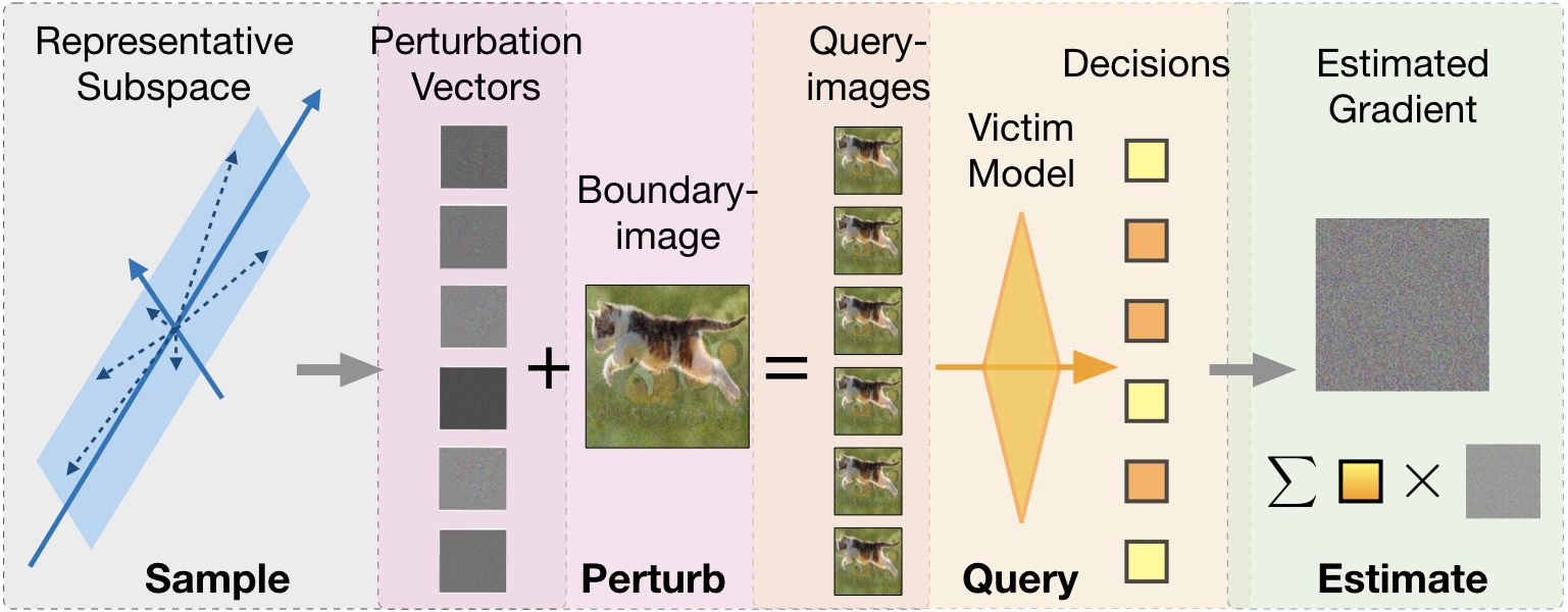
Figure 2: Query model and estimate gradient near the decision boundary.

Estimate gradient at decision boundary

Denote ${\bf x}_{adv}^{(t)}$ as the adv-image generated in the $t$-th step. The intuition in this step is that we can estimate the gradient of $S({\bf x}_{adv}^{(t)})$ using only the access to $\phi$ if ${\bf x}_{adv}^{(t)}$ is at the decision boundary. This gradient can be sampled via Monte Carlo method:

$$\widetilde{\nabla S}=\frac{1}{B}\sum_{i=1}^{B}\phi({\bf x}_{adv}^{(t)}+\delta{\bf u}_{b}){\bf u}_{b}$$ (3)

where $\{{\bf u}_{b}\}$ are $B$ randomly sampled perturbations with unit length and $\delta$ is a small weighting constant. An example of this process is shown in Figure 2. The key point here is how to sample the perturbation ${\bf u}_{b}$’s and we propose to draw from a representative subspace in $\mathbb{R}^{n}$.

Formally speaking, let $W=[w_{1},\ldots,w_{n}]\in\mathbb{R}^{m\times n}$ be $n$ orthonormal basis vectors in $\mathbb{R}^{m}$, meaning $W^{\intercal}W=I$. Let $\text{span}(W)\subseteq\mathbb{R}^{m}$ denote the $n$-dimensional subspace spanned by $w_{1},\ldots,w_{n}$. We would like to sample random perturbations from $\text{span}(W)$ instead of from the original space $\mathbb{R}^{m}$. In order to do that, we sample ${\bf v}_{b}\in\mathbb{R}^{n}$ from unit sphere in $\mathbb{R}^{n}$ and let ${\bf u}_{b}=W{\bf v}_{b}$. The detailed gradient estimation algorithm is shown in Alg.1. Note that if we let $\text{span}(W)=\mathbb{R}^{m}$, this step will be the same as in [9]. However, we will sample from some representative subspace so that the gradient estimation is more efficient, and the corresponding theoretic justification is discussed in Section 4.

Algorithm 1 Gradient Approximation Based QEBA

0:  a data point on the decision boundary ${\bf x}\in\mathbb{R}^{m}$, basis of the subspace $W\in\mathbb{R}^{m\times n}$, number of random sampling $B$, access to query the decision of victim model $\phi$.

0:  the approximated gradient $G$

1:  sample $B$ random Gaussian vectors of the lower dimension: $V_{rnd}\in\mathbb{R}^{B\times n}$.

2:  project the random vectors onto the gradient basis to get the perturbation vectors: $U_{rnd}=V_{rnd}\cdot W^{\intercal}$.

3:  get query points by adding perturbation vectors with the original point on the decision boundary: ${\bf x}_{q}[i]={\bf x}+U_{rnd}[i]$.

4:  Monte Carlo approximation for the gradient: $G=\frac{1}{B}\sum_{i=1}^{B}\phi({\bf x}_{q}[i])\cdot U_{rnd}[i]$

5:  return  $G$

Move along estimated gradient

After we have estimated the gradient of adversarial prediction score $\nabla S$, we will move the ${\bf x}_{adv}^{(t)}$ towards the gradient direction:

$$\hat{\bf x}_{t+1}={\bf x}_{adv}^{(t)}+\xi_{t}\cdot\frac{\widetilde{\nabla S}}{||\widetilde{\nabla S}||_{2}}$$ (4)

where $\xi_{t}$ is the step size at the $t$-th step. Hence, the prediction score of the adversarial class will be increased.

Project to decision boundary

Current $\hat{\bf x}_{t+1}$ is beyond the boundary, we can move the adv-image towards the target image so that it is projected back to the decision boundary:

$${\bf x}_{adv}^{(t+1)}=\alpha_{t}\cdot{\bf x}_{tgt}+(1-\alpha_{t})\cdot\hat{\bf x}_{t+1}$$ (5)

where the projection is achieved by a binary search over $\alpha_{t}$.

Note that we assume ${\bf x}_{adv}^{(t)}$ lies on the boundary while ${\bf x}_{src}$ does not lie on the boundary. Therefore, in the initialization step we need to first apply a project operation as in Eqn. 5 to get ${\bf x}_{adv}^{(0)}$.

In the following sections, we will introduce three exploration for the representative subspace optimization from spatial, frequency, and intrinsic component perspectives.

3.2 Spatial Transformed Subspace (QEBA-S)

First we start with the spatial transformed query reduction approach. The intuition comes from the observation that the gradient of input image has a property of local similarity[20]. Therefore, a large proportion of the gradients lies on the low-dimensional subspace spanned by the bilinear interpolation operation[34]. In order to sample random perturbations for an image, we first sample a lower-dimensional random perturbation $Q$ of shape $\lfloor\frac{N}{r}\rfloor\times\lfloor\frac{N}{r}\rfloor$, where $r$ is the hyperparameter of dimension reduction factor. Then we use bilinear-interpolation to map it back the original image space, $X=\text{Bil\_Interp}(Q)$.

The basis of this spatial transformed subspace is the images transformed from unit perturbations in the lower space:

$$w^{(i,j)}=\text{Bil\_Interp}(e^{(i,j)}),\quad 0\leq i,j\leq\lfloor N/r\rfloor$$

where $e^{(i,j)}$ represents the unit vector that has 1 on the $(i,j)$-th entry and 0 elsewhere.

3.3 Low Frequency Subspace (QEBA-F)

In general the low frequency subspace of an image contains the most of the critical information, including the gradient information[15]; while the high frequency signals contain more noise than useful content. Hence, we would like to sample our perturbations from the low frequency subspace via Discrete Cosine Transformation(DCT)[1]. Formally speaking, define the basis function of DCT as:

$$\phi(i,j)=\cos\bigg{(}\frac{(i+\frac{1}{2})j}{N}\pi\bigg{)}$$ (6)

The inverse DCT transformation is a mapping from the frequency domain to the image domain $X=\text{IDCT}(Q)$:

$$X_{i_{1},i_{2}}=\sum_{j_{1}=0}^{N-1}\sum_{j2=0}^{N-1}N_{j_{1}}N_{j_{2}}Q_{j_{1},j_{2}}\phi(i_{1},j_{1})\phi(i_{2},j_{2})$$ (7)

where $N_{j}=\sqrt{1/N}$ if $j=0$ and otherwise $N_{j}=\sqrt{2/N}$.

We will use the lower $\lfloor N/r\rfloor$ part of the frequency domain as the subspace, i.e.

$$w^{(i,j)}=\text{IDCT}(e^{(i,j)}),\quad 0\leq i,j\leq\lfloor N/r\rfloor$$ (8)

where hyperparameter $r$ is the dimension reduction factor.

3.4 Intrinsic Component Subspace (QEBA-I)

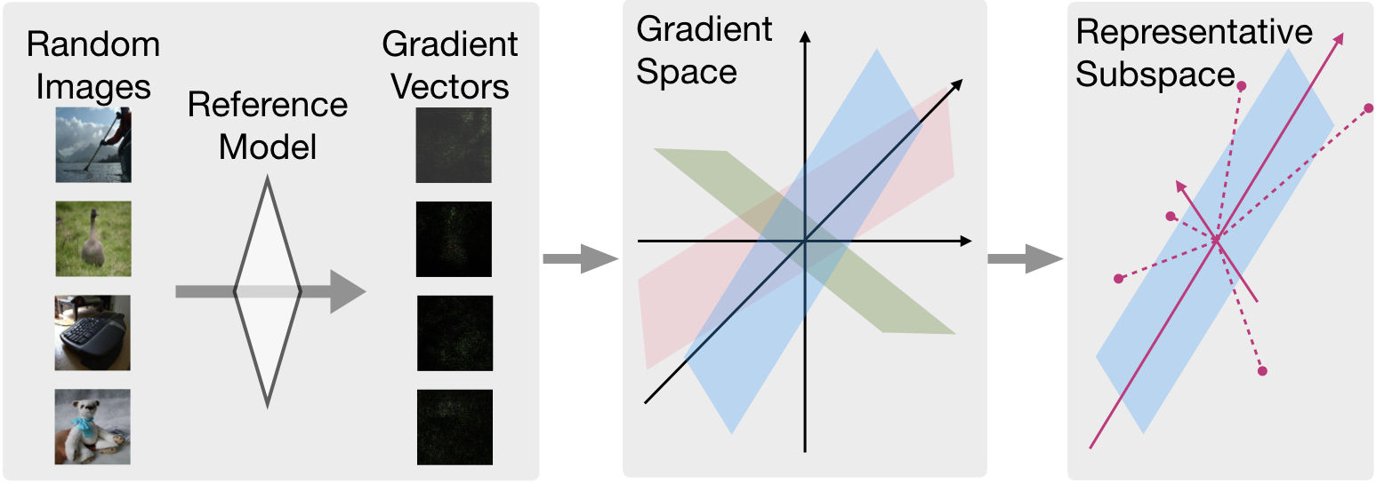
Figure 3: Generate representative subspace from the original high-dimensional gradient space.

Principal Component Analysis (PCA)[39] is a standard way to perform dimension reduction in order to search for the intrinsic components of the given instances. Given a set of data points in high dimensional space, PCA aims to find a lower dimensional subspace so that the projection of the data points onto the subspace is maximized.

Therefore, it is possible to leverage PCA to optimize the subspace for model gradient matrix. However, in order to perform PCA we will need a set of data points. In our case that should be a set of gradients of $S({\bf x})$ w.r.t. different $\bf x$. This is not accessible under black-box setting. Hence, we turn to a set of ‘reference models’ to whose gradient we have access. As shown in Figure 3, we will use a reference model to calculate a set of image gradients ${\bf g}_{1},{\bf g}_{2},\ldots,{\bf g}_{K}\in\mathbb{R}^{m}$ Then we perform a PCA to extract its top-$n$ principal components - ${\bf w}_{1},\ldots,{\bf w}_{n}\in\mathbb{R}^{m}$. These $w$’s are the basis of the Intrinsic Component Subspace. Note that different from transferability, we do not restrict the reference models to be trained by the same training data with the original model, since we only need to search for the intrinsic components of the give dataset which is relatively stable regarding diverse models.

In practice, the calculation of PCA may be challenging in terms of time and memory efficiency based on large high-dimensional dataset (the data dimension on ImageNet is over 150k and we need a larger number of data points, all of which are dense). Therefore, we leverage the randomized PCA algorithms[16] which accelerates the speed of PCA while achieving comparable performance.

An additional challenge is that the matrix $X$ may be too large to be stored in memory. Therefore, we store them by different rows since each row (i.e. gradient of one image) is calculated independently with the others. The multiplication of $X$ and other matrices in memory are then implemented accordingly.

4 Theoretic Analysis on QEBA

We theoretically analyze how dimension reduction helps with the gradient estimation in QEBA. We show that the gradient estimation bound is tighter by sampling from a representative subspace rather than the original space.

We consider the gradient estimation as in Eqn. 3 and let $\rho=\frac{||\text{proj}_{\text{span}(W)}(\nabla S)||_{2}}{||\nabla S||_{2}}$ denote the proportion of $\nabla S$ that lies on the chosen subspace $\text{span}(W)$. Then we have the following theorem on the expectation of the cosine similarity between $\nabla S$ and estimated $\widetilde{\nabla S}$:

Theorem 1.

Suppose 1) $S({\bf x})$ has $L$-Lipschitz gradients in a neighborhood of $\bf x$, 2) the sampled ${\bf v}_{1},\ldots,{\bf v}_{B}$ are orthogonal to each other, and 3) $W^{\intercal}W=I$, then the expected cosine simliarity between $\widetilde{\nabla S}$ and $\nabla S$ can be bounded by:

$$\bigg{(}2\bigg{(}1-(\frac{L\delta}{2||\nabla S||_{2}})^{2}\bigg{)}^{\frac{n-1}{2}}-1\bigg{)}c_{n}\rho\sqrt{\frac{B}{n}}$$ (9)

$$\leq \mathbb{E}\big{[}\cos(\widetilde{\nabla S},\nabla S)\big{]}$$ (10)

$$\leq c_{n}\rho\sqrt{\frac{B}{n}}$$ (11)

where $c_{n}$ is a coefficient related with the subspace dimension $n$ and can be bounded by $c_{n}\in(2/\pi,1)$. In particular:

$$\lim_{\delta\rightarrow 0}\mathbb{E}\big{[}\cos(\widetilde{\nabla_{W}S},\nabla S)\big{]}=c_{n}\rho\sqrt{\frac{B}{n}}.$$ (12)

The theorem proof is in Appendix A. If we sample from the entire space (i.e. $\text{span}(W)=\mathbb{R}^{m}$), the expected cosine similarity is $c_{m}\sqrt{\frac{B}{m}}$. If we let $m=3\times 224\times 224$ and $B=100$, the similarity is only around 0.02.

On the other hand, if the subspace basis $w$’s are randomly chosen, then $\rho\approx\sqrt{\frac{n}{m}}$ and the estimation quality is low. With larger $\rho$, the estimation quality will be better than sampling from the entire space. Therefore, we further explore three approaches to optimize the representative subspace that contains a larger portion of the gradient as discussed in Section 3. For example, in the experiments we see that when $n=m/16$, we can reach $\rho=0.5$ and the expected cosine similarity increase to around 0.06. This improves the gradient estimation quality which leads to more efficient attacks.

5 Experiments

In this section, we introduce our experimental setup and quantitative results of the proposed methods QEBA-S, QEBA-F, and QEBA-I, compared with the HSJA attack[9], which is the-state-of-the-art boundary-based blackbox attack. Here we focus on the strongest baseline HSJA, which outperforms all of other Boundary Attack [2], Limited Attack [19] and Opt Attack [10] by a substantial margin. We also show two sets of qualitative results for attacking two real-world APIs with the proposed methods.

5.1 Datasets and Experimental Setup

Datasets

We evaluate the attacks on two offline models on ImageNet[11] and CelebA[24] and two online face recognition APIs Face++[26] and Azure[28]. We use a pretrained ResNet-18 model as the target model for ImageNet and fine-tune a pretrained ResNet-18 model to classify among 100 people in CelebA. We randomly select 50 pairs from the ImageNet/CelebA validation set that are correctly classified by the model as the source and target images.

Attack Setup

Following the standard setting in [9], we use $\xi_{t}=||{\bf x}_{adv}^{(t-1)}-{\bf x}_{tgt}||_{2}/\sqrt{t}$ as the size in each step towards the gradient. We use $\delta_{t}=\frac{1}{m}||{\bf x}_{adv}^{(t-1)}-{\bf x}_{tgt}||_{2}$ as the perturbation size and $B=100$ queries in the Monte Carlo algorithm to estimate the gradient, where $m=3\times 224\times 224$ is the input dimension in each Monte Carlo step.

We provide two evaluation metrics to evaluate the attack performance. The first is the average Mean Square Error (MSE) curve between the target image and the adversarial example in each step, indicating the magnitude of perturbation. The smaller the perturbation is, the more similar the adversarial example is with the target-image, thus providing better attack quality. The second is the attack success rate based on a limited number of queries, where the ‘success’ is defined as reaching certain specific MSE threshold. The less queries we need in order to reach a certain perturbation threshold, the more efficient the attack method is.

As for the dimension-reduced subspace, we use the dimension reduction factor $r=4$ in spatial transformed and low frequency subspace, which gives a 9408 dimensional subspace. In order to generate the Intrinsic Component Subspace, we first generate a set of image gradient vectors on the space. We average over the gradient of input w.r.t. five different pretrained substitute models - ResNet-50[17], DenseNet-121[18], VGG16[33], WideResNet[41] and GoogleNet[36]. We use part of the ImageNet validation set (280000 images) to generate the gradient vectors. Finally we adopt the scalable approximate PCA algorithm[16] to extract the top 9408 major components as the intrinsic component subspace.

5.2 Commercial Online APIs

Various companies provide commercial APIs (Application Programming Interfaces) of trained models for different tasks such as face recognition. Developers of downstream tasks can pay for the services and integrate the APIs into their applications. Note that although typical platform APIs provide the developers the confidence score of classes associated with their final predictions, the end-user using the final application would not have access to the scores in most cases. For example, some of Face++’s partners use the face recognition techniques for log-in authentication in mobile phones [27], where the user only knows the final decision (whether they pass the verification or not).

We choose two representative platforms for our real-world experiments based on only the final prediction. The first is Face++ from MEGVII[26], and the second is Microsoft Azure[28]. Face++ offers a ‘compare’ API [26] with which we can send an HTTPS request with two images in the form of byte strings, and get a prediction confidence of whether the two images contain the same person. In all the experiments we consider a confidence greater than 50% meaning the two images are tagged as the same person. Azure has a slightly more complicated interface. To compare two images, each image first needs to pass a ‘detect’ API call [28] to get a list of detected faces with their landmarks, features, and attributes. Then the features of both images are fed into a ‘verify’ function [29] to get a final decision of whether they belong to the same person or not. The confidence is also given, but we do not need it for our experiments since we only leverage the binary prediction for practical purpose.

In the experiments, we use the examples in Figure 4 as source-image and target-image. More specifically, we use a man-woman face as the source-target pair for the ‘compare’ API Face++, and we use a cat-woman face as the pair for the ‘detect’ API Azure face detection.

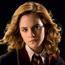
(a) Person 1

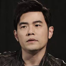
(b) Person 2

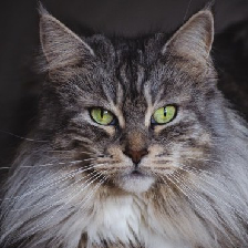
(c) No-face

Figure 4: The source and target images for online API experiments. All images are resized to $3\times 224\times 224$. Image 4(a) is the target-image for both APIs. Image 4(b) is the source-image for attacking Face++ ‘compare’ API, and 4(c) the source-image for Azure ‘detect’ API.

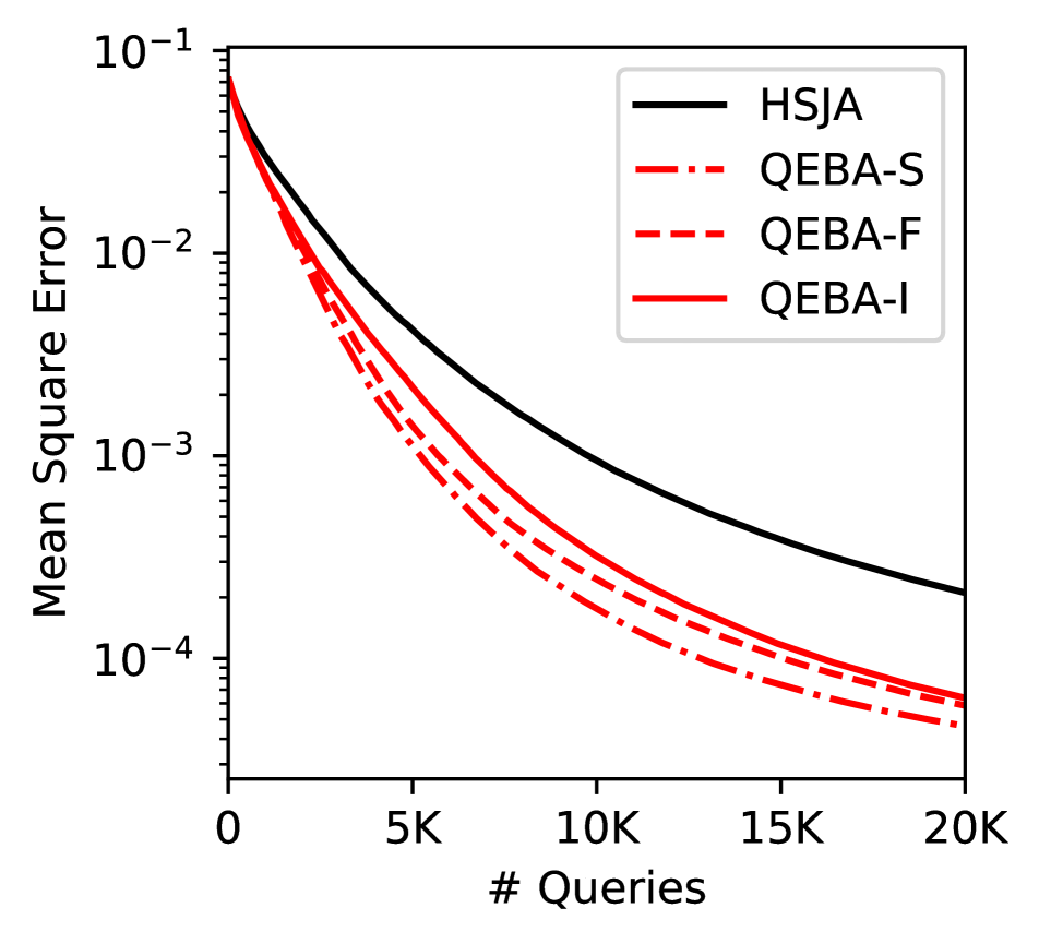
(a) The MSE vs. query number on ImageNet.

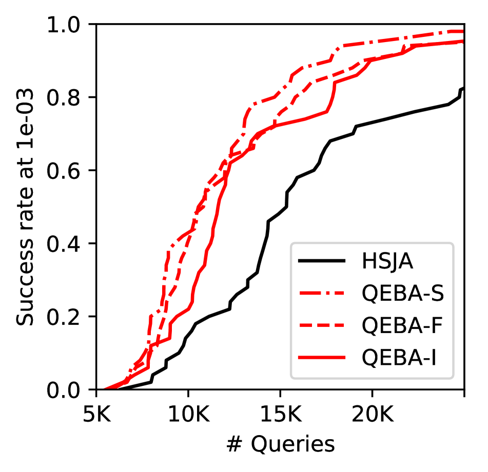
(b) The attack success rate with threshold $10^{-3}$ on ImageNet.

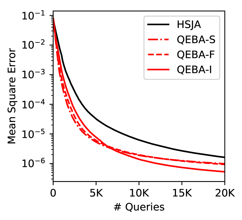
(c) The MSE vs. query number on CelebA.

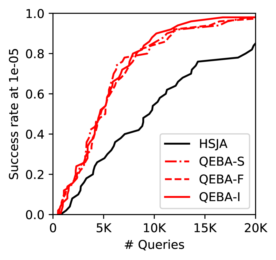
(d) The attack success rate with threshold $10^{-5}$ on CelebA.

Figure 5: The attack results on ImageNet and CelebA datasets.

Discretization Optimization for Attacking APIs

The attack against online APIs suffers from the problem of ‘discretization’. That is, in the attack process we assume the pixel values to be continuous in $[0,1]$, but we need to round it into 8-bit floating point in the uploaded RGB images when querying the online APIs. This would cause error in the Monte Carlo gradient estimation format in Equation 3 since the real perturbation between the last boundary-image and the new query image after rounding is different from the weighted perturbation vector $\delta{\bf u}_{b}$.

In order to mitigate this problem, we perform discretization locally. Let $P_{rd}$ be a projection from a continuous image $\bf x_{c}$ to a discrete image $\bf x_{d}=P_{rd}(\bf x_{c})$. Let $\delta{\bf u^{\prime}}_{b}=P_{rd}(\bf x+\delta{\bf u}_{b})-x$, the new gradient estimation format becomes:

$$\widetilde{\nabla f} =\frac{1}{B}\sum_{i=1}^{B}\phi(P_{rd}({\bf x}+\delta{\bf u}_{b})){\bf u^{\prime}}_{b}.$$ (13)

5.3 Experimental Results on Offline Models

Table 1: Attack success rate using different number of queries and different MSE thresholds.

		# Queries = 5000				# Queries = 10000				# Queries = 20000
	MSE threshold	HJSA	-S	QEBA -F	-I	HJSA	-S	QEBA -F	-I	HJSA	-S	QEBA -F	-I
ImageNet	0.01	0.76	0.86	0.86	0.86	0.98	1.00	0.96	0.98	1.00	1.00	1.00	1.00
	0.001	0.16	0.40	0.42	0.36	0.50	0.74	0.76	0.74	0.84	0.98	0.96	0.98
	0.0001	0.02	0.08	0.06	0.04	0.06	0.32	0.30	0.20	0.28	0.70	0.66	0.68
CelebA	0.01	0.96	1.00	1.00	0.96	1.00	1.00	1.00	1.00	1.00	1.00	1.00	1.00
	0.001	0.90	1.00	1.00	0.94	0.98	1.00	1.00	1.00	1.00	1.00	1.00	1.00
	0.0001	0.76	0.96	0.96	0.90	0.90	1.00	1.00	1.00	1.00	1.00	1.00	1.00

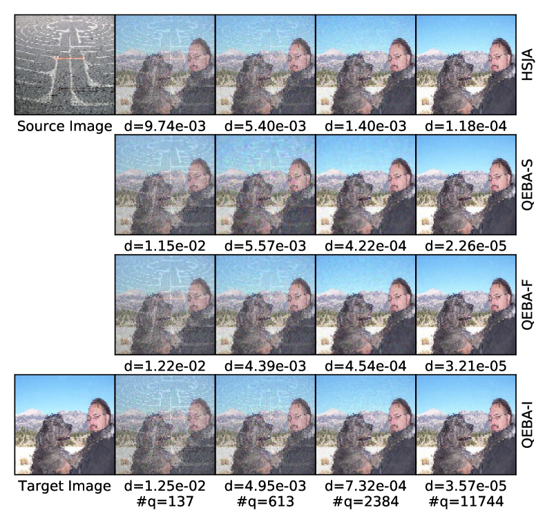
Figure 6: An example of attacking ImageNet trained model based on different subspaces.

To evaluate the effectiveness of the proposed methods, we first show the average MSE during the attack process of ImageNet and CelebA using different number of queries in Figure 5(a) and Figure 5(c) respectively. We can see that all the three proposed query efficient methods outperform HSJA significantly. We also show the attack success rate given different number of queries in Table 1 using different MSE requirement as the threshold. In addition, we provide the attack success rate curve in Figure 5(b) and 5(d) using $10^{-3}$ as the threshold for ImageNet and $10^{-5}$ for CelebA to illustrate convergence trend for the proposed QEBA-S, QEBA-F, and QEBA-I, comparing with the baseline HJSA.

We observe that sampling in the optimized subspaces results in a better performance than sampling from the original space. The spatial transforamed subspace and low-frequency subspace show a similar behaviour since both of them rely on the local continuity. The intrinsic component subspace does not perform better than the other two approaches, and the potential reason is that we are only using 280000 cases to find intrinsic components on the 150528-dimensional space. Therefore, the extracted components may not be optimal. We also observe that the face recognition model is much easier to attack than the ImageNet model, since the face recognition model has fewer classes (100) rather than 1000 as of ImageNet.

A qualitative example process of attacking the ImageNet model using different subspaces is shown in Figure 6. In this example, the MSE (shown as $d$ in the figures) reaches below $1\times 10^{-3}$ using around 2K queries when samlping from the subspaces, and it is already hard to tell the adversarial perturbations in the examples. When we further tune the adv-image using 10K queries, it reaches lower MSE.

5.4 Results of Attacking Online APIs

The results of attacking online APIs Face++ and Azure are shown in Figure 7 and Figure 8 respectively. The labels on the y-axis indicate the methods. Each column represents successful attack instances with increasing number of API calls. As is the nature of boundary-based attack, all images are able to produce successful attack. The difference lies in the quality of attack instances.

For attacks on Face++ ‘compare’ API, the source-image is a man and the target-image is a woman as shown in Figure 4. Notice the man’s eyes appear in a higher position in the source-image than the woman in the target-image because of the pose. All the instances on the first row in Figure 7 based on HJSA attacks contain two pairs of eyes. The MSE scores ($d$ in the figures) also confirm that the distance between the attack instance and the target-image does not go down much even with more than 6000 queries. On the other hand, our proposed methods QEBA- can optimize attack instances with smaller magnitude of perturbation more efficiently. The perturbations are also smoother.

The attack results on Azure ‘detect’ API show similar observations. The source-image is a cat and the target-image is the same woman. Sampling from the original high-dimensional space (HJSA) gives us attack instances that presents two cat ear shapes at the back of the human face as shown in the first row in Figure 8. With the proposed query efficient attacks, the perturbations are smoother. The distance metric ($d$) also demonstrates the superiority of the proposed methods.

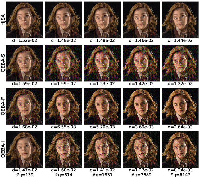
Figure 7: Comparison of attacks on Face++ ‘compare’ API. Goal: obtain an image that is tagged as ‘same person’ with the source-image person 2 (Figure 4(b)) by the API when humans can clearly see person 1 here.

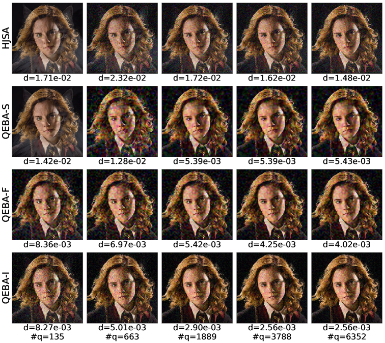
Figure 8: Comparison of attacks on Azure ‘detect’ API. Goal: get an image that is tagged as ‘no face’ by the API when humans can clearly see a face there. The source-image is a cat as shown in Figure 4(c).

6 Related Work

Boundary-based Attack

Boundary Attack [2] is one of the first work that uses final decisions of a classifier to perform blackbox attacks. The attack process starts from the source-image, which is classified as the adversarial malicious-class. Then it employs a reject sampling mechanism to find a boundary-image that still belongs to the malicious-class by performing random walk along the boundary. The goal is to minimize the distance between the boundary-image and the target-image. However, as the steps taken are randomly sampled, the convergence of this method is slow and the query number is large.

Several techniques have been proposed to improve the performance of Boundary Attack. [3, 35, 15] propose to choose the random perturbation in each step more wisely instead of Gaussian perturbation, using Perlin noise, alpha distribution and DCT respectively. [19, 21, 23, 9] propose a similar idea - approximating the gradient around the boundary using Monte Carlo algorithm.

There are two other blackbox attacks which are not based on the boundary. [10] proposes to transform the boundary-based output into a continuous metric, so that the score-based attack techniques can be adopted. [12] adopts evolution algorithm to achieve the decision-based attack against face recognition system.

Dimension Reduction in Score-based Attack

Another line of work involves the dimension reduction techniques only for the score-based attacks, which requires access to the prediction of confidence for each class. In [15], the authors draw intuition from JPEG codec [38] image compression techniques and propose to use discrete cosine transform (DCT) for generating low frequency adversarial perturbations to assist score-based adversarial attack. AutoZoom [37] trains an auto-encoder offline with natural images and uses the decoder network as a dimension reduction tool. Constrained perturbations in the latent space of the auto-encoder are generated and passed through the decoder. The resulting perturbation in the image space is added to the benign one to obtain a query sample.

7 Conclusion

Overall we propose QEBA, a general query-efficient boundary-based blackbox attack framework. We in addition explore three novel subspace optimization approaches to reduce the number of queries from spatial, frequency, and intrinsic components perspectives. Based on our theoretic analysis, we show the optimality of the proposed subspace based gradient estimation compared with the estimation over the original space. Extensive results show that the proposed QEBA significantly reduces the required number of queries and yields high quality adversarial examples against both offline and onlie real-world APIs.

Acknowledgement

We would like to thank Prof. Yuan Qi and Prof. Le Song for their comments and advice in this project. This work is partially supported by NSF grant No.1910100.

Appendix A Proof of Theorem 1

We first prove a lemma of the gradient estimation quality which samples from the entire subspace:

Lemma 1.

For a boundary point $x$, suppose that $S(x)$ has $L$-Lipschitz gradients in a neighborhood of $x$, and that ${\bf u}_{1},\ldots,{\bf u}_{B}$ are sampled from the unit ball in $\mathbb{R}^{m}$ and orthogonal to each other. Then the expected cosine similarity between $\widetilde{\nabla S}$ and $\nabla S$ can be bounded by:

$$\bigg{(}2\bigg{(}1-(\frac{L\delta}{2||\nabla S||_{2}})^{2}\bigg{)}^{\frac{m-1}{2}}-1\bigg{)}c_{m}\sqrt{\frac{B}{m}}$$ (14)

$$\leq \mathbb{E}\big{[}\cos(\widetilde{\nabla S},\nabla S)\big{]}$$ (15)

$$\leq c_{m}\sqrt{\frac{B}{m}}$$ (16)

where $c_{m}$ is a constant related with $m$ and can be bounded by $c_{m}\in(2/\pi,1)$. In particular, we have:

$$\lim_{\delta\rightarrow 0}\mathbb{E}\big{[}\cos(\widetilde{\nabla S},\nabla S)\big{]}=c_{m}\sqrt{\frac{B}{m}}.$$ (17)

Proof.

Let ${\bf u}_{1},\ldots,{\bf u}_{B}$ be the random orthonormal vectors sampled from $\mathbb{R}^{m}$. We expand the vectors to an orthonormal basis in $\mathbb{R}^{m}$: ${\bf q}_{1}={\bf u}_{1},\ldots,{\bf q}_{B}={\bf u}_{B},{\bf q}_{B+1},\ldots,{\bf q}_{m}$. Hence, the gradient direction can be written as:

$$\frac{\nabla S}{||\nabla S||_{2}}=\sum_{i=1}^{m}a_{i}{\bf q}_{i}$$ (18)

where $a_{i}=\langle\frac{\nabla S}{||\nabla S||_{2}},{\bf q}_{i}\rangle$ and its distribution is equivalent to the distribution of one coordinate of an $(m-1)$-sphere. Then each $a_{i}$ follows the probability distribution function:

$$p_{a}(x)=\frac{(1-x^{2})^{\frac{m-3}{2}}}{\mathcal{B}(\frac{m-1}{2},\frac{1}{2})},~{}x\in(-1,1)$$ (19)

where $\mathcal{B}$ is the beta function. According to the conclusion in the proof of Theorem 1 in [9], if we let $w=\frac{L\delta}{2||\nabla S||_{2}}$, then it always holds true that $\phi({\bf x}+\delta{\bf u_{i}})=1$ when $a_{i}>w$, -1 when $a_{i}<-w$ regardless of $u_{i}$ and the decision boundary shape. Hence, we can rewrite $\phi_{i}$ in term of $a_{i}$:

$$\phi_{i}=\phi({\bf x}+\delta{\bf u_{i}})=\begin{cases}1,&\text{if }a_{i}\in[w,1)\\ -1,&\text{if }a_{i}\in(-1,-w]\\ \text{undetermined},&\text{otherwise}\end{cases}$$ (20)

Therefore, the estimated gradient can be rewritten as:

$$\widetilde{\nabla S}=\frac{1}{B}\sum_{i=1}^{B}\phi_{i}{\bf u}_{i}$$ (21)

Combining Eqn. 18 and 21, we can calculate the cosine similarity:

$$\mathop{\mathbb{E}}\big{[}\cos(\widetilde{\nabla S},\nabla S)\big{]} =\mathop{\mathbb{E}}_{a_{1},\ldots,a_{B}}\frac{\sum_{i=1}^{B}a_{i}\phi_{i}}{\sqrt{B}}$$ (22)

$$=\sqrt{B}\cdot\mathop{\mathbb{E}}_{a_{1}}\big{[}a_{1}\phi_{1}\big{]}$$ (23)

In the best case, $\phi_{1}$ has the same sign with $a_{1}$ everywhere on $(-1,1)$; in the worst case, $\phi_{1}$ has different sign with $a_{1}$ on $(-w,w)$. In addition, $p_{a}(x)$ is symmetric on $(-1,1)$. Therefore, the expectation is bounded by:

$$2\int_{w}^{1}p_{a}(x)\cdot xdx-2\int_{0}^{w}p_{a}(x)\cdot xdx$$ (24)

$$\leq \mathop{\mathbb{E}}_{a_{1}}\big{[}a_{1}\phi_{1}\big{]}$$ (25)

$$\leq 2\int_{0}^{1}p_{a}(x)\cdot xdx$$ (26)

By calculating the integration, we have:

$$\bigg{(}2\bigg{(}1-w^{2}\bigg{)}^{\frac{m-1}{2}}-1\bigg{)}\cdot\frac{2\sqrt{B}}{\mathcal{B}(\frac{m-1}{2},\frac{1}{2})\cdot(m-1)}$$ (27)

$$\leq \mathop{\mathbb{E}}\big{[}\cos(\widetilde{\nabla S},\nabla S)\big{]}$$ (28)

$$\leq \frac{2\sqrt{B}}{\mathcal{B}(\frac{m-1}{2},\frac{1}{2})\cdot(m-1)}$$ (29)

The only problem is to calculate $\mathcal{B}(\frac{m-1}{2},\frac{1}{2})\cdot(m-1)$. It is easy to prove by scaling that $\mathcal{B}(\frac{m-1}{2},\frac{1}{2})\cdot(m-1)\in(2\sqrt{m},\pi\sqrt{m})$. Hence we can get the conclusion in the theorem. ∎

Having Lemma 1, Theorem 1 follows by noticing that $\mathbb{E}\big{[}\cos(\widetilde{\nabla S},\nabla S)\big{]}=\rho\mathbb{E}\big{[}\cos(\widetilde{\nabla S},\text{proj}_{\text{span}(W)}(\nabla S))\big{]}$.

References

- [1] Nasir Ahmed, T_ Natarajan, and Kamisetty R Rao. Discrete cosine transform. IEEE transactions on Computers, 100(1):90–93, 1974.
- [2] Wieland Brendel, Jonas Rauber, and Matthias Bethge. Decision-based adversarial attacks: Reliable attacks against black-box machine learning models. arXiv preprint arXiv:1712.04248, 2017.
- [3] Thomas Brunner, Frederik Diehl, Michael Truong Le, and Alois Knoll. Guessing smart: Biased sampling for efficient black-box adversarial attacks. In Proceedings of the IEEE International Conference on Computer Vision, pages 4958–4966, 2019.
- [4] Nicholas Carlini and David Wagner. Towards evaluating the robustness of neural networks. In 2017 IEEE Symposium on Security and Privacy (SP), pages 39–57. IEEE, 2017.
- [5] Bo Li Fisher Yu Jinfeng Yi Mingyan Liu Chaowei Xiao, Duizhi Deng and Dawn Song. Characterizing adversarial examples based on spatial consistency information for semantic segmentation. In ECCV, 2018.
- [6] Bo Li Warren He Mingyan Liu Chaowei Xiao, Jun-Yan Zhu and Dawn Song. Spatially transformed adversarial examples. In ICLR, 2018.
- [7] Chenyi Chen, Ari Seff, Alain Kornhauser, and Jianxiong Xiao. Deepdriving: Learning affordance for direct perception in autonomous driving. In Proceedings of the IEEE International Conference on Computer Vision, pages 2722–2730, 2015.
- [8] Hongming Chen, Ola Engkvist, Yinhai Wang, Marcus Olivecrona, and Thomas Blaschke. The rise of deep learning in drug discovery. Drug discovery today, 23(6):1241–1250, 2018.
- [9] Jianbo Chen, Michael I Jordan, and Martin J Wainwright. Hopskipjumpattack: A query-efficient decision-based attack. arXiv preprint arXiv:1904.02144, 2019.
- [10] Minhao Cheng, Thong Le, Pin-Yu Chen, Jinfeng Yi, Huan Zhang, and Cho-Jui Hsieh. Query-efficient hard-label black-box attack: An optimization-based approach. arXiv preprint arXiv:1807.04457, 2018.
- [11] Jia Deng, Wei Dong, Richard Socher, Li-Jia Li, Kai Li, and Li Fei-Fei. Imagenet: A large-scale hierarchical image database. In 2009 IEEE conference on computer vision and pattern recognition, pages 248–255. Ieee, 2009.
- [12] Yinpeng Dong, Hang Su, Baoyuan Wu, Zhifeng Li, Wei Liu, Tong Zhang, and Jun Zhu. Efficient decision-based black-box adversarial attacks on face recognition. In Proceedings of the IEEE Conference on Computer Vision and Pattern Recognition, pages 7714–7722, 2019.
- [13] Kevin Eykholt, Ivan Evtimov, Earlence Fernandes, Bo Li, Amir Rahmati, Chaowei Xiao, Atul Prakash, Tadayoshi Kohno, and Dawn Song. Robust physical-world attacks on deep learning models. arXiv preprint arXiv:1707.08945, 2017.
- [14] Ian J Goodfellow, Jonathon Shlens, and Christian Szegedy. Explaining and harnessing adversarial examples. arXiv preprint arXiv:1412.6572, 2014.
- [15] Chuan Guo, Jared S Frank, and Kilian Q Weinberger. Low frequency adversarial perturbation. arXiv preprint arXiv:1809.08758, 2018.
- [16] Nathan Halko, Per-Gunnar Martinsson, and Joel A Tropp. Finding structure with randomness: Probabilistic algorithms for constructing approximate matrix decompositions. SIAM review, 53(2):217–288, 2011.
- [17] Kaiming He, Xiangyu Zhang, Shaoqing Ren, and Jian Sun. Deep residual learning for image recognition. In Proceedings of the IEEE conference on computer vision and pattern recognition, pages 770–778, 2016.
- [18] Gao Huang, Zhuang Liu, Laurens Van Der Maaten, and Kilian Q Weinberger. Densely connected convolutional networks. In Proceedings of the IEEE conference on computer vision and pattern recognition, pages 4700–4708, 2017.
- [19] Andrew Ilyas, Logan Engstrom, Anish Athalye, and Jessy Lin. Black-box adversarial attacks with limited queries and information. arXiv preprint arXiv:1804.08598, 2018.
- [20] Andrew Ilyas, Logan Engstrom, and Aleksander Madry. Prior convictions: Black-box adversarial attacks with bandits and priors. arXiv preprint arXiv:1807.07978, 2018.
- [21] Faiq Khalid, Hassan Ali, Muhammad Abdullah Hanif, Semeen Rehman, Rehan Ahmed, and Muhammad Shafique. Red-attack: Resource efficient decision based attack for machine learning. arXiv preprint arXiv:1901.10258, 2019.
- [22] Ian Lenz, Honglak Lee, and Ashutosh Saxena. Deep learning for detecting robotic grasps. The International Journal of Robotics Research, 34(4-5):705–724, 2015.
- [23] Yujia Liu, Seyed-Mohsen Moosavi-Dezfooli, and Pascal Frossard. A geometry-inspired decision-based attack. arXiv preprint arXiv:1903.10826, 2019.
- [24] Ziwei Liu, Ping Luo, Xiaogang Wang, and Xiaoou Tang. Large-scale celebfaces attributes (celeba) dataset.
- [25] Aleksander Madry, Aleksandar Makelov, Ludwig Schmidt, Dimitris Tsipras, and Adrian Vladu. Towards deep learning models resistant to adversarial attacks. arXiv preprint arXiv:1706.06083, 2017.
- [26] MEGVII. Facial recognition compare api. https://console.faceplusplus.com/documents/5679308.
- [27] MEGVII. Selected cases. https://megvii.com/selected_cases.
- [28] Microsoft. Faceoperations class detect_with_stream. https://tinyurl.com/t7ulxvx.
- [29] Microsoft. Faceoperations class verify_face_to_face. https://tinyurl.com/rlcayd2.
- [30] Shaoqing Ren, Kaiming He, Ross Girshick, and Jian Sun. Faster r-cnn: Towards real-time object detection with region proposal networks. In Advances in neural information processing systems, pages 91–99, 2015.
- [31] Florian Richter, Ryan K Orosco, and Michael C Yip. Open-sourced reinforcement learning environments for surgical robotics. arXiv preprint arXiv:1903.02090, 2019.
- [32] Kumba Sennaar. Machine learning in surgical robotics – 4 applications that matter. https://emerj.com/ai-sector-overviews/machine-learning-in-surgical-robotics-4-applications/.
- [33] Karen Simonyan and Andrew Zisserman. Very deep convolutional networks for large-scale image recognition. arXiv preprint arXiv:1409.1556, 2014.
- [34] Helmuth Späth. Two dimensional spline interpolation algorithms. CRC Press, 1993.
- [35] Vignesh Srinivasan, Ercan E Kuruoglu, Klaus-Robert Müller, Wojciech Samek, and Shinichi Nakajima. Black-box decision based adversarial attack with symmetric alpha-stable distribution. arXiv preprint arXiv:1904.05586, 2019.
- [36] Christian Szegedy, Wei Liu, Yangqing Jia, Pierre Sermanet, Scott Reed, Dragomir Anguelov, Dumitru Erhan, Vincent Vanhoucke, and Andrew Rabinovich. Going deeper with convolutions. In Proceedings of the IEEE conference on computer vision and pattern recognition, pages 1–9, 2015.
- [37] Chun-Chen Tu, Paishun Ting, Pin-Yu Chen, Sijia Liu, Huan Zhang, Jinfeng Yi, Cho-Jui Hsieh, and Shin-Ming Cheng. Autozoom: Autoencoder-based zeroth order optimization method for attacking black-box neural networks. In Proceedings of the AAAI Conference on Artificial Intelligence, volume 33, pages 742–749, 2019.
- [38] Gregory K Wallace. The jpeg still picture compression standard. IEEE transactions on consumer electronics, 38(1):xviii–xxxiv, 1992.
- [39] Svante Wold, Kim Esbensen, and Paul Geladi. Principal component analysis. Chemometrics and intelligent laboratory systems, 2(1-3):37–52, 1987.
- [40] Chaowei Xiao, Bo Li, Jun-Yan Zhu, Warren He, Mingyan Liu, and Dawn Song. Generating adversarial examples with adversarial networks. arXiv preprint arXiv:1801.02610, 2018.
- [41] Sergey Zagoruyko and Nikos Komodakis. Wide residual networks. arXiv preprint arXiv:1605.07146, 2016.