A moment matching method for option pricing under stochastic interest rates

Abstract

In this paper we present a simple, but new, approximation methodology for pricing a call option in a Black & Scholes market characterized by stochastic interest rates. The method, based on a straightforward Gaussian moment matching technique applied to a conditional Black & Scholes formula, is quite general and it applies to various models, whether affine or not. To check its accuracy and computational time, we implement it for the CIR interest rate model correlated with the underlying, using the Monte Carlo simulations as a benchmark. The method’s performance turns out to be quite remarkable, even when compared with analogous results obtained by the affine approximation technique presented in [9] and by the expansion formula introduced in [11], as we show in the last section.

Keywords: Option pricing, Stochastic interest rates, Moment matching, Non-affine models, Cox-Ingersoll-Ross model.

1 Introduction

Since the appearance of the seminal Black & Scholes/Merton option pricing fundamental formula, there has been an intensive effort to incorporate in the market model additional stochastic factors, such as the volatility and/or the interest rates, the latter already discussed by Merton himself in [15]. Along the years, a huge field of research developed, leading to a very rich literature on stochastic volatility models, while fewer papers aimed at the inclusion of a dynamic term structure into the valuation of derivatives, e.g. [17], [1], [20], [19], [11], [7], [18].

Nowadays, the improvement in the performances of option pricing formulas obtained by adding these risk factors is widely recognized in the empirical literature (see e.g [2], [3]), indeed in ([12]) the author remarked that even including solely stochastic interest rates in the model does affect the pricing formula, especially for longer-dated options, in a noticeable manner.

Of course this generalization implies a higher degree of mathematical complexity and the search for efficient pricing techniques, able to provide accurate answers in a short computational time (as opposed to Monte Carlo methods) has been relentless, even more so in modern quantitative finance where a huge amount of data allows to consider strategies that call for on real-time model calibration. Hence, computational efficiency has become one of the primary concerns of risk managers and this requirement essentially restricted the choice of models to the affine class (see [7]).

Indeed, when the interest rates are modeled in a Gaussian processes framework, as in the very popular Hull-White / Vasicek models, even analytical prices can be obtained. These models are appropriate for modeling periods that admit positive probability of negative rates, such as the current one, but this feature becomes a drawback in usual periods of positive rates. The most popular model used to avoid this drawback is the Cox-Ingersoll-Ross (CIR) one, which guarantees the rate’s strict positivity under Feller’s condition. Its popularity comes from the fact that falls into the so called affine models, that can exploit a very efficient and fast Fourier transform technique to price the bonds.

Unfortunately, the affinity of the model is lost when the interest rate is coupled, with correlation, with a risky asset’s dynamics, making the search for efficient approximations of risk-neutral pricing formulas very challenging.

Here we present a simple, but new, approximation methodology for pricing a European call option in a market model given by a linear diffusion dynamics for the underlying (a Black & Scholes (BS) framework) coupled with a stochastic short term risk-free rate. The problem is a classical one and the novelty lies on the fact that we propose a quite straightforward moment matching (MM) technique, easy to implement and leading to very efficient approximations.

In building our procedure a few issues have to be addressed and we first provide, by appropriate conditioning, a representation formula for the claim’s price in terms of the BS formula, then we exploit a Gaussian approximation by properly matching the first two moments of the involved random variables, that allows to use the properties of the Normal cumulative distribution function (c.d.f.) (see Lemma (1)). When applying the method to the affine models, we also employ a change-of-numeraire technique (introducing the $T$-forward measure as in [5]) to partially disentangle the contributions due to the underlying and to the interest rate, exploiting the explicit expressions of the bond’s price in an affine framework. To keep computations as simple as possible, any time a quantity is computable, it is stored and treated as a constant in the sequel. This leads to an efficient mixed use of the risk free probability and the $T$-forward measure to evaluate the separate quantities.

The paper is organized as follows. In Section 2 we derive a representation formula for the call option’s price in Black & Scholes market with stochastic risk-free short rates, while in Section 3 the Moment Matching method is fully described. Finally, in Section 4 we restrict to the affine models and we apply our technique with a CIR interest rate. In the same Section, we briefly introduce other two techniques, the affine approximation, inspired by Grzelak and Oosterlee [9] and the expansion method proposed by Kim and Kunimoto [11] alternative to prices obtained by Monte Carlo simulations. Hence we run a numerical study comparing those methods with ours, using Monte Carlo evaluation as a benchmark.

2 The price of a European call in the BS model with stochastic rates

The underlying problem we are concerned with is the pricing of a European call option, whose payoff is given by the function $f(x)=(\mathrm{e}^{x}-\mathrm{e}^{\kappa})^{+}$ for some $\kappa\in\mathbb{R}$, when stochastic interest rates come into play.

Thus, given a finite time interval $[0,T]$ and a complete probability space $(\Omega,{\mathcal{F}},Q)$, endowed of a filtration $\{{\mathcal{F}}_{t}\}_{\{t\in[0,T]\}}$ satisfying the “usual hypotheses” (see [16]), the market model is defined by the log-price of a risky asset and a risk-free interest $(X_{t},r_{t})$, whose joint dynamic for any initial condition $(t,x,r)\in[0,T]\times\mathbb{R}\times\mathbb{R}$ and $\forall s\in[t,T]$ is given by

$$\!\!\begin{cases}X_{s}=X_{t}+\!\int_{t}^{s}(r_{v}\!-\frac{\sigma^{2}}{2})dv+\sigma\Big{[}\rho(B_{s}^{1}\!-B^{1}_{t})+\sqrt{1\!-\!\rho^{2}}(B^{2}_{s}-B_{t}^{2})\Big{]},\,\,\,X_{t}=x\\ r_{s}=r_{t}+\int_{t}^{s}\mu(v,r_{v})dv+\int_{t}^{s}\eta(v,r_{v})dB^{1}_{v},\quad r_{t}=r,\end{cases}$$ (1)

where $(B^{1},B^{2})$ is a two dimensional standard Brownian motion and $\rho\in(-1,1)$. Moreover, we assume that the deterministic functions $\mu(\cdot,\cdot)$ and $\eta(\cdot,\cdot)$ are in a class that ensures the existence and uniqueness of a strong solution of (1) (see e.g. [10]) and that $Q$ is some risk neutral probability selected by the market.

Under these assumptions, the pair $(X_{t},r_{t})$ is Markovian, whence the arbitrage-free option’s price is a deterministic function of the state variables, given by

$$u(t,x,r,T;\rho)=\mathbb{E}(\mathrm{e}^{-\int_{t}^{T}r_{s}}(\mathrm{e}^{X_{T}(\rho)}-\mathrm{e}^{\kappa})^{+}ds|X_{t}=x,r_{t}=r),$$ (2)

provided that the coefficients $\mu$ and $\eta$ are chosen to guarantee the exponential integrability of $X_{T}$ and $\int_{0}^{T}|r_{s}|ds$. Here we wrote $X_{T}(\rho)$, to stress the prices’ dependence on the correlation parameter.

If $u(t,x,r,T;\rho)$ is regular enough in $t,x,r$, Feymann-Kac’s formula implies that it is a classical solution of the following two-dimensional parabolic problem

$$\begin{cases}\frac{\partial u}{\partial t}+{{\mathcal{L}}^{\rho}}u=0\\ u(T,x,r,T;\rho)=(\mathrm{e}^{x}-\mathrm{e}^{\kappa})^{+},\end{cases}$$ (3)

where ${\mathcal{L}}^{\rho}={\mathcal{L}}^{\mathbf{0}}+{\mathcal{A}}$, with

$${\mathcal{L}}^{\mathbf{0}} := \biggl{(}\frac{\sigma^{2}}{2}\frac{\partial^{2}}{\partial x^{2}}+(r-\frac{\sigma^{2}}{2})\frac{\partial}{\partial x}-r\biggr{)}+\biggl{(}\frac{\eta^{2}(t,r)}{2}\frac{\partial^{2}}{\partial r^{2}}+\mu(t,r)\frac{\partial}{\partial r}\biggr{)}$$ (4)

$${\mathcal{A}} := \rho\sigma\eta(t,r)\frac{\partial^{2}}{\partial x\partial r}.$$ (5)

In what follows to keep notation easy, we take $t=0$ and we omit the dependence on $t$ in the pricing function. The general case may be readily obtained substituting $T$ in the final formulas with the time to maturity $T-t$.

By conditioning internally with respect to ${\mathcal{F}}^{1}_{T}=\sigma(\{B^{1}_{s}:0\leq s\leq T\})$, we have

$$u(x,r,T;\rho)=\mathbb{E}\left(\mathrm{e}^{-\int_{0}^{T}r_{s}ds}(\mathrm{e}^{X_{T}(\rho)}-\mathrm{e}^{\kappa})^{+}\right)=\mathbb{E}\left(\mathrm{e}^{-\int_{0}^{T}r_{s}ds}\mathbb{E}\big{(}(\mathrm{e}^{X_{T}(\rho)}-\mathrm{e}^{\kappa})^{+}|{\mathcal{F}}^{1}_{T}\big{)}\right).$$ (6)

But $X_{T}(\rho)\big{|}{\mathcal{F}}^{1}_{T}\sim N(M_{T},\Sigma_{T})$, where

$$M_{T}=x+\int_{0}^{T}(r_{s}-\frac{\sigma^{2}}{2})ds+\sigma\rho B_{T}^{1},\quad\text{and}\quad\Sigma^{2}_{T}=\sigma(1-\rho^{2})T.$$

so we obtain

$$\mathbb{E}\left((\mathrm{e}^{X_{T}(\rho)}-\mathrm{e}^{\kappa})^{+}|{\mathcal{F}}^{1}_{T}\right)= \mathrm{e}^{M_{T}+\frac{1}{2}\Sigma_{T}^{2}}{\mathcal{N}}\left(\frac{M_{T}-\kappa+\Sigma_{T}^{2}}{\Sigma_{T}}\right)-\mathrm{e}^{\kappa}{\mathcal{N}}\left(\frac{M_{T}-\kappa}{\Sigma}\right)$$

$$= \mathrm{e}^{x+\int_{0}^{T}(r_{s}-\frac{\sigma^{2}}{2})ds+\sigma\rho B_{T}^{1}+\frac{1}{2}\sigma^{2}(1-\rho^{2})T}{\mathcal{N}}(d_{1}(\rho))-\mathrm{e}^{\kappa}{\mathcal{N}}(d_{2}(\rho)),$$

where we define

$$d_{1}(\rho) = \frac{x-\kappa+\int_{0}^{T}r_{s}ds+\sigma\rho B^{1}_{T}+\frac{\sigma^{2}}{2}T-\sigma^{2}\rho^{2}T}{\sigma\sqrt{1-\rho^{2}}\sqrt{T}}$$ (7)

$$d_{2}(\rho) = \frac{x-\kappa+\int_{0}^{T}r_{s}ds+\sigma\rho B^{1}_{T}-\frac{\sigma^{2}}{2}T}{\sigma\sqrt{1-\rho^{2}}\sqrt{T}}$$ (8)

and ${\mathcal{N}}$ denotes the cumulative distribution function of the standard Gaussian. It is convenient to introduce the following notations

$$\Lambda_{T}=\int_{0}^{T}r_{s}ds,\;\;\;\beta(T,\rho)=\frac{\rho}{(1-\rho^{2})^{1/2}\sqrt{T}},\;\,\gamma(T,\rho)=\frac{1}{\sigma(1-\rho^{2})^{1/2}\sqrt{T}}$$

$$\alpha_{1}(x,T,\rho)=\frac{x-\kappa+\frac{\sigma^{2}}{2}T-\sigma^{2}\rho^{2}T}{\sigma(1-\rho^{2})^{1/2}\sqrt{T}},\;\;\;\alpha_{2}(x,T,\rho)=\frac{x-\kappa-\frac{\sigma^{2}}{2}T}{\sigma(1-\rho^{2})^{1/2}\sqrt{T}},$$

so that

$$d_{i}(x,T,\rho)=\alpha_{i}(x,T,\rho)+\beta(T,\rho)B_{T}^{1}+\gamma(T,\rho)\Lambda_{T},\quad i=1,2.$$ (9)

Setting $S_{T}=\mathrm{e}^{-\Lambda_{T}}$, we can finally write

$$u(x,r,T;\rho)=\mathrm{e}^{x}\mathrm{e}^{-\frac{\sigma^{2}\rho^{2}}{2}T}\mathbb{E}\left(\mathrm{e}^{\sigma\rho B_{T}^{1}}{\mathcal{N}}\big{(}d_{1}(\rho)\big{)}\right)-\mathrm{e}^{\kappa}\mathbb{E}\left(S_{T}{\mathcal{N}}\big{(}d_{2}(\rho)\big{)}\right).$$ (10)

In the forthcoming section we shall introduce the moment matching approximation procedure.

3 Option price approximation by moment matching

The main idea of this section is to replace the r.v.’s $d_{i}(\rho)$, $i=1,2$, defined by (9), with Gaussian r.v.’s $D_{i}(\rho)$ matching the first and second moments of $d_{i}(\rho)$.

We define

$$D_{i}(\rho):=\alpha_{i}(x,T,\rho)+\hat{\beta}(T,\rho)B_{T}^{1}+\gamma(T,\rho)\mathbb{E}(\Lambda_{T}),\;\;\;i=1,2,$$

consequently

$$\mathbb{E}\big{(}D_{i}(\rho)\big{)}=\alpha_{i}(x,T,\rho)+\gamma(T,\rho)\mathbb{E}(\Lambda_{T})=\mathbb{E}\big{(}d_{i}(\rho)\big{)}$$ (11)

and the new coefficient $\hat{\beta}>0$ is fixed such that

$$\mathrm{var}\big{(}D_{i}(\rho)\big{)}= T\hat{\beta}^{2}(T,\rho)=\mathrm{var}(d_{1}(\rho))=\mathrm{var}(d_{2}(\rho))$$ (12)

$$= \beta^{2}(T,\rho)T+\gamma^{2}(T,\rho)\mathrm{var}(\Lambda_{T})+2\beta(T,\rho)\gamma(T,\rho)\mathbb{E}(B_{T}^{1}\Lambda_{T})$$

with

$$\mathrm{var}(\Lambda_{T}) = \mathbb{E}\left(\Big{(}\int_{0}^{T}r_{s}ds\Big{)}^{2}\right)-\Big{[}\mathbb{E}\left(\int_{0}^{T}r_{s}ds\right)\Big{]}^{2},$$ (13)

$$\mathbb{E}(B_{T}^{1}\Lambda_{T}) = \mathbb{E}\left(B_{T}^{1}\int_{0}^{T}r_{s}ds\right).$$ (14)

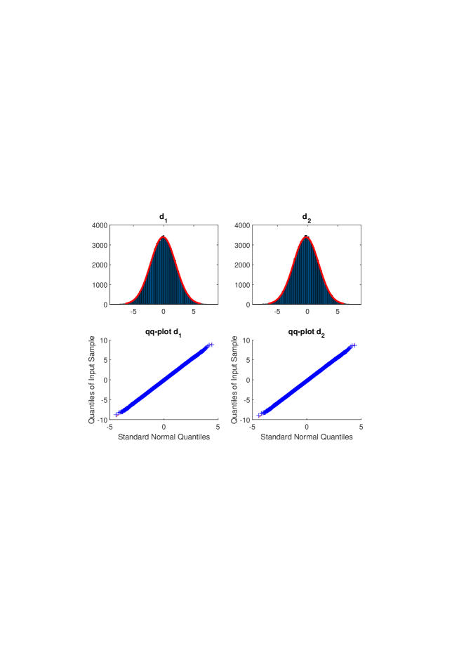
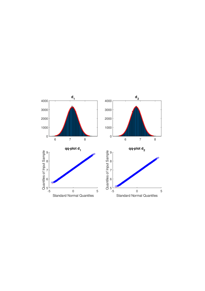
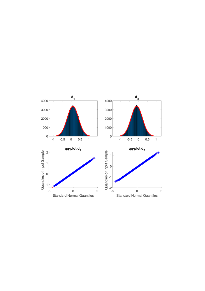
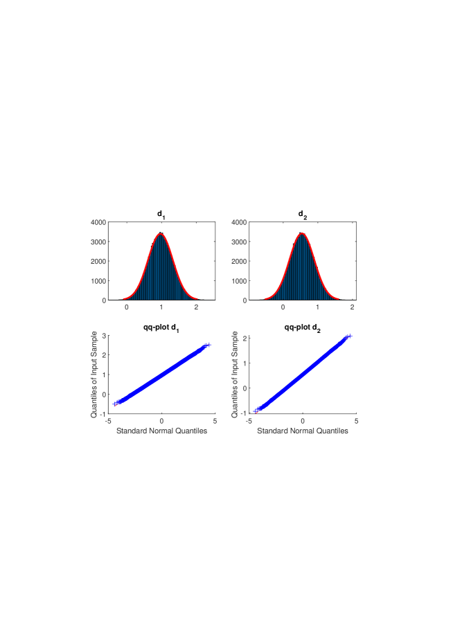
The moment matching method with Gaussian r.v’s may be motivated by looking at the empirical distributional properties of the random variables $d_{i}$ in some well-known rate models: see as examples Figs (1), (2) and (3).

We finally introduce a call price approximation

$$u^{appr}(x,r,T;\rho):= \mathrm{e}^{x}\mathrm{e}^{-\frac{1}{2}\sigma^{2}\rho^{2}T}\mathbb{E}\left(\mathrm{e}^{\sigma\rho B_{T}^{1}}{\mathcal{N}}\big{(}D_{1}(\rho)\big{)}\right)-\mathrm{e}^{\kappa}\mathbb{E}\left(S_{T}{\mathcal{N}}\big{(}D_{2}(\rho)\big{)}\right)$$ (15)

$$=: \mathrm{e}^{x}\mathrm{e}^{-\frac{1}{2}\sigma^{2}\rho^{2}T}\ F(\rho)-\mathrm{e}^{\kappa}G(\rho).$$

The function $F$ can be evaluated in closed form by means of the following

Lemma 1

Let $p\in\mathbb{\mathbb{R}}$ and $X\sim N(\mu,\nu^{2})$, $(\mu,\nu)\in\mathbb{R}\times\mathbb{R}^{+}$, then

$$\mathbb{E}(\mathrm{e}^{pX}{\mathcal{N}}(X))=\mathrm{e}^{p\mu+\frac{(p\nu)^{2}}{2}}{\mathcal{N}}\biggl{(}\frac{\mu+p\nu^{2}}{\sqrt{1+\nu^{2}}}\biggr{)}.$$

Proof: See [21] for $p=0$, the general case follows by a “completing the squares” argument. $\square$

Since

$$B_{T}^{1}=\big{[}D_{1}(\rho)-\alpha_{1}(x,T,\rho)-\gamma(T,\rho)\mathbb{E}(\Lambda_{T})\big{]}\hat{\beta}(T,\rho)^{-1},$$

we may rewrite $F$ as

$$F(\rho)= \mathbb{E}\left(\mathrm{e}^{\sigma\rho(D_{1}(\rho)-\alpha_{1}(x,T,\rho)-\gamma(T,\rho)\mathbb{E}(\Lambda_{T}))\hat{\beta}(T,\rho)^{-1}}{\mathcal{N}}(D_{1}(\rho))\right)$$

$$= \mathrm{e}^{-\sigma\rho[\alpha_{1}(x,T,\rho)+\gamma(T,\rho)\mathbb{E}(\Lambda_{T})]\hat{\beta}(T,\rho)^{-1}}\mathbb{E}\left(\mathrm{e}^{\sigma\rho D_{1}(\rho)\hat{\beta}(T,\rho)^{-1}}{\mathcal{N}}(D_{1}(\rho))\right)$$

$$= \mathrm{e}^{-\sigma\rho[\alpha_{1}(x,T,\rho)+\gamma(T,\rho)\mathbb{E}(\Lambda_{T})]\hat{\beta}(T,\rho)^{-1}}\mathrm{e}^{\sigma\rho\mathbb{E}(D_{1}(\rho))\hat{\beta}(T,\rho)^{-1}+\frac{\hat{\beta}(T,\rho)^{-2}\sigma^{2}\rho^{2}\mathrm{var}(D_{1}(\rho))}{2}}$$

$$\times{\mathcal{N}}\Big{(}\frac{\mathbb{E}(D_{1}(\rho))+\sigma\rho\mathrm{var}(D_{1}(\rho))\hat{\beta}(T,\rho)^{-1}}{\sqrt{1+\mathrm{var}(D_{1}(\rho))}}\Big{)}.$$

From (11) and (12), we may conclude

$$F(\rho)=\mathrm{e}^{\frac{\sigma^{2}\rho^{2}T}{2}}{\mathcal{N}}\left(\frac{\alpha_{1}(x,T,\rho)+\sigma\rho\hat{\beta}(T,\rho)T+\gamma(T,\rho)\mathbb{E}(\Lambda_{T})}{\sqrt{1+\hat{\beta}^{2}(T,\rho)T}}\right).$$ (16)

If $\mathbb{E}(\Lambda_{T})$ and (13), (14) can be computed, then $F$ is totally explicit. From now on, we denote $\lambda(T):=\mathbb{E}(\Lambda_{T})$ to point out this is a known constant.

On the contrary, the function $G$ cannot be evaluated in such a straightforward manner, as it involves a detailed knowledge of the joint distribution of $\Lambda_{T}$ and $B^{1}_{T}$ and not only of their moments and covariance. So, to represent $G$, we suggest applying a a change-of-numeraire technique that allows us to exploit the bond pricing theory.

Let us define

$$P(s,T):=\mathbb{E}\left((\mathrm{e}^{-\int_{s}^{T}r_{v}dv}|{\mathcal{F}}_{s}\right),$$ (17)

the Zero Coupon Bond price. Again, since $r.$ is a Markov process, $P(s,T)$ is a deterministic function of the state variable, say $g(s,r_{s})$, which we assume to be ${\mathcal{C}}^{1,2}([0,T]\times\mathbb{R}^{+})$. For $0\leq s\leq T$, we define the ${\mathcal{F}}_{s}$-martingale (we remark that is a true martingale thanks to the exponential integrability of $\Lambda_{T}$)

$$L_{s}=\frac{\mathbb{E}(\mathrm{e}^{-\int_{0}^{T}r_{v}dv}|{\mathcal{F}}_{s})}{P(0,T)}=S_{s}\frac{P(s,T)}{P(0,T)}=S_{s}\frac{g(s,r_{s})}{g(0,r)},\quad r_{0}=r.$$ (18)

By applying Itô’s formula, we have the dynamic of $L$

$$dL_{s}= \frac{S_{s}}{g(0,r)}\Big{[}\frac{\partial g}{\partial t}(s,r_{s})+\frac{1}{2}\eta^{2}(s,r_{s})\frac{\partial^{2}g}{\partial r^{2}}(s,r_{s})+\mu(s,r_{s})\frac{\partial g}{\partial r}(s,r_{s})-r_{s}g(s,r_{s})\Big{]}ds$$

$$+ \frac{S_{s}}{g(0,r)}\eta(s,r_{s})\frac{\partial g}{\partial r}(s,r_{s})dB^{1}_{s}=\frac{S_{s}}{g(0,r)}\eta(s,r_{s})\frac{\partial g}{\partial r}(s,r_{s})dB^{1}_{s},\quad L_{0}=1$$

and we may define the $T$-forward measure on every $A\in{\mathcal{F}}$ by $Q^{T}(A):=\mathbb{E}(L_{T}1_{A})$ (see [4] for the method and [6] for a similar application). Under $Q^{T}$, we get

$$G(\rho)=\mathbb{E}\left(S_{T}{\mathcal{N}}(D_{2}(\rho))\right)=P(0,T)\mathbb{E}^{Q^{T}}\left({\mathcal{N}}(D_{2}(\rho))\right),$$ (19)

and by Girsanov theorem, by setting

$$\xi_{s}:=\int_{0}^{s}\frac{\eta(v,r_{v})}{g(v,r_{v})}\frac{\partial g}{\partial r}(v,r_{v})dv,$$

we have that the process $\tilde{B}^{1}_{s}:=B^{1}_{s}-\xi_{s}$ is a $Q^{T}-$Brownian motion. When choosing an interest rate model that allows an explicit expression of the bond’s price, $\mathbb{E}^{Q^{T}}\left({\mathcal{N}}(D_{2}(\rho))\right)$ will be the last quantity to compute. Under $Q^{T}$, $D_{2}(\rho)$ has the expression

$$D_{2}(\rho)=\alpha_{2}(x,T,\rho)+\xi_{T}\hat{\beta}(T,\rho)+\hat{\beta}(T,\rho)\tilde{B}_{T}^{1}+\gamma(T,\rho)\lambda(T),$$

whence its distribution is no longer known.

To compute the final expectation, we replace $D_{2}(\rho)$ by the r.v.

$$\bar{D}_{2}(\rho):=\alpha_{2}(x,T,\rho)+\mathbb{E}(\xi_{T})\hat{\beta}(T,\rho)+\hat{\beta}(T,\rho)\tilde{B}_{T}^{1}+\gamma(T,\rho)\lambda(T),$$

where we are taking $\epsilon(T):=\mathbb{E}(\xi_{T})$ under the original probability $Q$, so that $\bar{D}_{2}(\rho)$ is a Gaussian r.v. and we may apply Lemma 1 once again to obtain

$$\mathbb{E}^{Q^{T}}({\mathcal{N}}(\bar{D}_{2}(\rho)))={\mathcal{N}}\left(\frac{\mathbb{E}^{Q^{T}}(\bar{D}_{2}(\rho))}{\sqrt{1+\mathrm{var}^{Q^{T}}(\bar{D}_{2}(\rho))}}\right),$$

with

$$\mathbb{E}^{Q^{T}}(\bar{D}_{2}(\rho))=\alpha_{2}(x,T,\rho)+\epsilon(T)\hat{\beta}(T,\rho)+\gamma(T,\rho)\lambda(T),\ \ \mathrm{var}^{Q^{T}}(\bar{D}_{2}(\rho))=\hat{\beta}^{2}(T,\rho)T.$$

Hence we shall denote by

$$\bar{G}(\rho):=P(0,T)\mathbb{E}^{Q^{T}}({\mathcal{N}}(\bar{D}_{2}(\rho)))$$

the approximation of $G(\rho)$ and we may define the final approximation of the call option price $u(x,r,T;\rho)$ as

$$\bar{u}(x,r,T;\rho):=\mathrm{e}^{x-\frac{1}{2}\sigma^{2}\rho^{2}T}F(\rho)-\mathrm{e}^{\kappa}\bar{G}(\rho)$$

$$= \mathrm{e}^{x}{\mathcal{N}}\left(\frac{\alpha_{1}(x,T,\rho)+\sigma\rho\hat{\beta}(T,\rho)T+\gamma(T,\rho)\lambda(T)}{\sqrt{1+\hat{\beta}^{2}(T,\rho)T}}\right)$$

$$- \mathrm{e}^{\kappa}P(0,T){\mathcal{N}}\left(\frac{\alpha_{2}(x,T,\rho)+\epsilon(T)\hat{\beta}(T,\rho)+\gamma(T,\rho)\lambda(T)}{\sqrt{1+\hat{\beta}^{2}(T,\rho)T}}\right).$$

As a conclusion, we summarize the key requirements to make the approximation (3) explicitly computable and hopefully efficient

1. the distributions of $d_{i}(\rho),i=1,2$ should be close to a Gaussian distribution;

2. the bond price $P(t,T)$ should be theoretically computable. Moreover one can exploit the observed (today) bond price for $P(0,T)$ in (18) and for calibration purposes;

3. the quantities $\mathbb{E}(\Lambda_{T})$, $\mathrm{var}(\Lambda_{T})$ and $\mathbb{E}(\Lambda_{T}B^{1}_{T})$ and/or their approximations, should be easily computable;

4. the change of numeraire technique (Girsanov’s theorem) should be applicable.

The performance of this approximation needs to be compared with Monte-Carlo simulated prices and then with other methods present in the literature. This will be done in the next section.

4 Numerics and comparison with other methodologies

In this section we employ an affine model for the interest rate. This choice provides an explicit expression for the the ZCB’s price (17). So our market model is given by

$$X_{s}= X_{t}+\!\!\int_{t}^{s}(r_{v}-\frac{\sigma^{2}}{2})dv+\sigma\Big{[}\rho(B_{s}^{1}\!-B^{1}_{t})+\sqrt{1\!-\!\rho^{2}}(B^{2}_{s}-B_{t}^{2})\Big{]},\quad X_{t}=x$$ (21)

$$r_{s}= r_{t}+\!\!\int_{t}^{s}[a(v)r_{v}+b(v)]dv+\int_{t}^{s}[c(v)r_{v}+d(v)]^{1/2}dB^{1}_{v},\quad r_{t}=r,$$

where $a,b,c,d:[0,T]\longrightarrow\mathbb{R}$ are bounded functions. In this framework, we have for $r_{t}=r$

$$P(t,T)=g(t,r)=A(t,T)\mathrm{e}^{-rB(t,T)},$$

for suitable deterministic functions $A(\cdot,T)$ and $B(\cdot,T)$. Two very classical models fall into this setting

$$\begin{aligned} \text{(Vasicek) }\quad&a(v)=-\gamma,\quad b(v)=\gamma\theta,\quad c(v)=0,\quad d(v)=\eta^{2}\\ \text{(CIR) }\quad&a(v)=-\gamma,\quad b(v)=\gamma\theta,\quad c(v)=\eta^{2},\quad d(v)=0\end{aligned}\quad\gamma,\theta>0,$$

for which $A(t,T)$ and $B(t,T)$ are explicitly known ([5]), the same being true also for the Hull-White / Vasicek and Hull-White / CIR models, considering time dependent coefficients.

The functions $A$ and $B$ are usually characterized by the solution of a Riccati system of ODE’s. Unfortunately, when in presence of correlation, the same procedure cannot be applied to the pair $(X.,r.)$, since its diffusion matrix

$$\sigma(v,x,r)\sigma(v,x,r)^{T}=\begin{pmatrix}\sigma^{2}&\rho\sigma[c(v)r+d(v)]^{1/2}\\ \rho\sigma[c(v)r+d(v)]^{1/2}&c(v)r+d(v)\end{pmatrix}$$ (22)

may haves entries which are non-linear in the state variables, so that the joint diffusion is no longer affine, as it happens for the CIR model. Hence, in this context it makes sense to apply the approximation procedure presented in the previous section. As before we consider $t=0$.

In this case (see e.g. [5]), setting $\delta=\sqrt{\gamma^{2}+2\eta^{2}}$, we have

$$A(0,T)=\mathrm{e}^{\frac{2\gamma\theta}{\eta^{2}}}\frac{2\delta\mathrm{e}^{\gamma+\delta T}}{\delta-\gamma+(\delta+\gamma)\mathrm{e}^{\delta T}},\quad B(0,T)=\frac{2(\mathrm{e}^{\delta T}-1)}{\delta-\gamma+(\delta+\gamma)\mathrm{e}^{\delta T}},$$

and let us proceed to the computation of $\mathbb{E}(\Lambda_{T})$, $\mathrm{var}(\Lambda_{T})$ and $\mathbb{E}(\Lambda_{T}B^{1}_{T})$.

1. Computation of $\mathbb{E}(\Lambda_{T})$. It is straightforward to see

   $$\mathbb{E}(\Lambda_{T})=\int_{0}^{T}\mathbb{E}(r_{s})ds=\int_{0}^{T}\big{[}(r_{0}-\theta)\mathrm{e}^{-\gamma s}+\theta\big{]}ds=\theta T+(r_{0}-\theta)\frac{1-\mathrm{e}^{-\gamma T}}{\gamma}.$$

2. Computation of $\mathrm{var}(\Lambda_{T})$. Taking into account the first point, we only have to compute the second moment

   $$\mathbb{E}\left(\Big{(}\!\!\int_{0}^{T}\!\!\!r_{s}ds\Big{)}^{2}\right)= \mathbb{E}\left(\int_{0}^{T}\!\!\!\int_{0}^{T}\!\!\!r_{s}r_{v}dsdv\right)=\int_{0}^{T}\!\!\!\int_{0}^{T}\mathbb{E}(r_{s}r_{v})dsdv$$

   $$= \int_{0}^{T}\!\!\!\int_{0}^{t}\mathbb{E}(r_{s}r_{v})dsdv+\int_{0}^{T}\!\!\!\int_{t}^{T}\mathbb{E}(r_{s}r_{v})dsdv$$

   $$= \int_{0}^{T}\!\!\!\int_{0}^{t}\!\!\!\mathbb{E}(r_{s}r_{v})dsdv+\!\!\int_{0}^{T}\!\!\!\int_{0}^{s}\!\!\!\mathbb{E}(r_{s}r_{v})dvds=2\!\!\int_{0}^{T}\!\!\!\int_{0}^{s}\!\!\!\mathbb{E}(r_{s}r_{v})dvds.$$

   By the independence of the increments of the process $r$, for $v<s$ we have

   $$\mathbb{E}(r_{s}r_{v})=\mathbb{E}\left((r_{s}-r_{v})r_{v}+r^{2}_{v}\right)=\mathbb{E}(r_{s}-r_{v})\mathbb{E}(r_{v})+\mathbb{E}(r_{v}^{2})$$

   $$= \mathbb{E}\Big{(}\theta(s-v)+(r_{v}-\theta)\frac{1-\mathrm{e}^{-\gamma(s-v)}}{\gamma}\Big{)}\mathbb{E}(r_{v})+\mathbb{E}(r_{v}^{2})$$

   $$= \theta\Big{[}(s-v)-\frac{1-\mathrm{e}^{-\gamma(s-v)}}{\gamma}\Big{]}\mathbb{E}(r_{v})+\frac{1-\mathrm{e}^{-\gamma(s-v)}}{\gamma}[\mathbb{E}(r_{v})]^{2}+\text{var}(r_{v})+[\mathbb{E}(r_{v})]^{2}$$

   Since $\mathrm{var}(r_{s})=r_{0}\frac{\eta^{2}}{\gamma}(\mathrm{e}^{-\gamma s}-\mathrm{e}^{-2\gamma s})+\frac{\theta\eta^{2}}{2\gamma}(1-\mathrm{e}^{-\gamma s})^{2}$, all the integrals appearing in the second moment can be calculated analytically.

3. Computation of $\mathbb{E}(B_{T}^{1}\Lambda_{T})$. By Itô’s integration-by-parts formula, we get

   $$\mathbb{E}(B_{T}^{1}\Lambda_{T})=\int_{0}^{T}\mathbb{E}(B_{s}^{1}r_{s})ds$$

   and again by integration by parts we have

   $$B^{1}_{s}r_{s}= \int_{0}^{s}B^{1}_{v}dr_{v}+\int_{0}^{s}r_{v}dB^{1}_{v}+\langle B^{1},r\rangle_{s}$$

   $$= \int_{0}^{s}B^{1}_{v}\gamma(\theta-r_{v})dt+\eta\int_{0}^{s}B^{1}_{t}\sqrt{r_{v}}dB^{1}_{v}+\int_{0}^{s}r_{v}dB^{1}_{v}+\eta\int_{0}^{s}\sqrt{r_{v}}dv,$$

   so that

   $$\mathbb{E}(B^{1}_{s}r_{s})=-\gamma\int_{0}^{s}\mathbb{E}(B^{1}_{v}r_{v})dv+\eta\int_{0}^{s}\mathbb{E}(\sqrt{r_{v}})dv.$$

   Solving this linear ODE for $h(s):=\mathbb{E}(B^{1}_{s}r_{s})$, since $h(0)=0$, we obtain

   $$\mathbb{E}(B^{1}_{s}r_{s})= \eta\int_{0}^{s}\mathrm{e}^{-\gamma(s-v)}\mathbb{E}(\sqrt{r_{v}})dv,$$

   $$\mathbb{E}(B_{T}^{1}\Lambda_{T})= \eta\int_{0}^{T}\int_{0}^{s}\mathrm{e}^{-\gamma(s-v)}\mathbb{E}(\sqrt{r_{v}})dvds.$$

   Thus the final crucial point is computing $\mathbb{E}(\sqrt{r_{v}})$, which is rather delicate (see [8]). No explicit expression can be provided and we employ the approximation proposed in [9], that we are going to present in the next subsection

   $$\mathbb{E}(\sqrt{r_{v}})\approx a+b\mathrm{e}^{-cv}$$ (23)

   where the parameters $a,b$ and $c$ are obtained by an ad hoc matching procedure, which proved to be numerically very efficient.

Finally, given the above three points, $\hat{\beta}(T,\rho)$ is easily computed from (12).

As a last step, we have to approximate $\mathbb{E}(\xi_{T})$, which is readily done, given the last remark, since

$$\mathbb{E}(\xi_{T})= \mathbb{E}\Big{(}-\eta\int_{0}^{T}\!\!\!B(s,T)\sqrt{r_{s}}ds\Big{)}=\mathbb{E}\Big{(}-\eta\int_{0}^{T}B(s,T)\mathbb{E}\big{(}\sqrt{r_{s}}\big{)}ds\Big{)}$$

$$\approx -\eta\int_{0}^{T}B(s,T)(a+b\mathrm{e}^{-cs})ds.$$

4.1 The Grzelak-Oosterlee (GO) approximation

Here and in the next subsection, for completeness, we briefly describe the two approximation techniques, we are going to compare with.

The GO approximation consists simply in modifying the ${\mathcal{A}}$ operator given in (5) by replacing the state variable in the coefficient with a constant, namely we define

$${\mathcal{A}}^{GO}u(s,x,r):=\rho\sigma\mathbb{E}(\eta(s,r_{t}s)\frac{\partial^{2}u}{\partial x\partial r}.$$

In the case of the CIR model, $\eta$ is time-homogeneous and this operator becomes

$${\mathcal{A}}^{GO}u(s,x,r):=\rho\sigma\eta\mathbb{E}(\sqrt{r_{s}}))\frac{\partial^{2}u}{\partial x\partial r}\approx\rho\sigma\eta(a+b\mathrm{e}^{-cs})\frac{\partial^{2}u}{\partial x\partial r}$$

Once this replacement has been made then the Fourier transform methods apply, hence it is possible to compute approximated prices of the call option. We shall denote this approximation by $u^{GO}(t,x,r,T;\rho)$. To evaluate the accuracy of this approximation a comparison with the prices of the (non-affine) true model, obtained by MC simulations, must be performed.

Once again we specialize the formulas for $t=0$ for a direct comparison with our results, so $X_{0}=x$ and $r_{0}=r$.

The discounted transform, for $\zeta\in\mathbb{C}$, (see [7]) for the affine approximation is

$$\phi(\zeta,x,r,T):=\mathbb{E}\left(\mathrm{e}^{-\int_{0}^{T}r_{s}ds}\mathrm{e}^{\zeta X_{T}}\right)=\mathrm{e}^{A(\zeta,T)+B(\zeta,T)x+C(\zeta,T)r},$$

where the functions $A,B,C$ satisfy a system of solvable ODE’s, that give

$$B(\zeta,T)= \zeta,$$

$$C(\zeta,T)= \frac{1-\mathrm{e}^{-dT}}{\eta^{2}(1-g\mathrm{e}^{-dT})},\ \ d=\sqrt{\gamma^{2}+2\eta^{2}(1-\zeta)},\ \ g=\frac{\gamma-d}{\gamma+d},$$

$$A(\zeta,T)= -\frac{\sigma^{2}}{2}T\zeta(1+\zeta)+\frac{\gamma-d}{\eta}\int_{0}^{T}\Big{[}\frac{\gamma\theta}{\eta}+\rho\sigma\zeta\overline{r^{sq}_{s}}\Big{]}\frac{1-\mathrm{e}^{-ds}}{(1-g\mathrm{e}^{-ds})}ds,$$

where $\overline{r}^{sq}_{s}=\mathbb{E}(\sqrt{r_{s}})$ is approximated as in (23).

Finally, by Lévy inversion formula as in [7] or Fourier inversion as in [13], one gets an integral representation for the price function: in our implementation we use the Fourier inversion

$$u^{GO}(x,r,T;\rho)=\frac{\mathrm{e}^{\nu\gamma}}{\pi}\int_{0}^{+\infty}\mathcal{R}\left(\frac{\mathrm{e}^{-\mathrm{i}\zeta\gamma}}{\nu^{2}-\nu-\zeta^{2}+\mathrm{i}\zeta(1-2\nu)}\phi(\zeta,x,r,T)\right)d\zeta,$$ (24)

where $\nu<0$ is a dumping factor and $\mathcal{R}(z)$ is the real part for $z\in\mathbb{C}$.

4.2 The Kim-Kunimoto (KK) approximation

Kim and Kunimoto, in [11], consider a Taylor expansion of the process $r_{s}$ in powers of $\eta$ around $\eta=0$. Considering the first order polynomial and setting $\varphi(s)=r\exp(-\gamma s)+\theta(1-\exp(-\gamma s))$, they obtain

$$r_{s}=\varphi(s)+\eta\int_{0}^{s}\mathrm{e}^{-\gamma(s-v)}\sqrt{\varphi(v)}(\rho dB^{1}_{v}+\sqrt{1-\rho^{2}}dB^{2}_{v})+o(\eta).$$ (25)

Inserting the approximation (25) in the evaluation formula for the call option, after some manipulations one can approximate the option’s price as

$$u^{KK}(x,r,T;\rho)= \mathrm{e}^{x}{\mathcal{N}}(d_{1})-\mathrm{e}^{\kappa-\int_{0}^{T}\varphi(s)ds}{\mathcal{N}}(d_{2})$$ (26)

$$+ \eta C_{1}\Big{[}d_{2}\mathrm{e}^{x}{\mathcal{N}}^{\prime}(d_{1})-d_{1}\mathrm{e}^{\kappa-\int_{0}^{T}\varphi(s)ds}{\mathcal{N}}^{\prime}(d_{2})\Big{]}$$

where

$$C_{1}= -\frac{\rho}{\sigma T}\frac{2\sqrt{\theta}\big{[}(1+2\mathrm{e}^{\gamma T})\sqrt{r}-3\gamma_{K}\big{]}+\big{[}r-\theta(1+2e^{\gamma T})\big{]}\lambda_{K}}{2\mathrm{e}^{\gamma T}\gamma^{2}\sqrt{\theta}},$$

$$d_{1}= \frac{x-\kappa+\theta T+(r-\theta)(1-\mathrm{e}^{-\gamma T})/\gamma+\sigma^{2}T/2}{\sqrt{\sigma^{2}T}},\ \ d_{2}=d_{1}-\sigma\sqrt{T},$$

being $\gamma_{K}=\mathrm{e}^{\gamma T/2}\sqrt{r-\theta(1-\mathrm{e}^{\gamma T})}$ and $\lambda_{K}=\log\left(\frac{(\sqrt{r}+\sqrt{\theta})^{2}}{r-\theta(1-2\mathrm{e}^{\gamma T})+2\gamma_{K}\sqrt{\theta})}\right)$.

4.3 Numerical results

We compare the results of the different approximations with the benchmark Monte Carlo method, applied to the price (10). In particular this means that we only have to simulate the rate process to get samples from $d_{1}(\rho)$ and $d_{2}(\rho)$. The simulation was implemented by means of the Euler discretization with full truncation algorithm (see [14]). In our numerical experiments we generated $M=10^{6}$ sample paths with a time step discretization equal to $10^{-3}$ for all the maturities. All the algorithms were implemented in MatLab (R2019b) and ran on an Intel Core i7 2.40GHZ with 8GB RAM, by using the available building-in functions, in particular for the computation of all the integrals involved. The average time to compute one price was (in secs) $32.1$ (MC), $0.055$ (GO), $0.005$ (KK) and $0.009$ (MM).

We chose different set of parameters $(\kappa,\theta,\eta)$ and volatility scenarios: a low volatility $\sigma_{L}=0.2$ and a high volatility $\sigma_{L}=0.4$; hence we varied the correlation $\rho$, the rate volatility $\eta$ and the maturity of the contract $T$. The initial price of the underlying was set to $100$ as well as the strike price $K$. Numerical results are summarized in Tables (1) - (8). At least in the CIR model, the numerical results show that the MM method produces the best approximations with respect to the benchmark Monte Carlo evaluation in most scenarios.

Figure 1: The histograms of $d_{1}$ and $d_{2}$ for $\rho=0.3$, $T=1$ (left) and $T=5$ (right), in comparison with the standard normal law (in red) and related qq-plot, CIR dynamic: $dr_{t}=\kappa(\theta-r_{t})dt+\eta\sqrt{r_{t}}dB^{1}_{t}$.

Figure 2: The histograms of $d_{1}$ and $d_{2}$ for $\rho=0.3$, $T=1$ (left) and $T=5$ (right), in comparison with the standard normal law (in red) and related qq-plot, Exponential Vasicek dynamic: $dr_{t}=r_{t}(\theta-a\ln(r_{t}))dt+\eta r_{t}dB^{1}_{t}$.

Figure 3: The histograms of $d_{1}$ and $d_{2}$ for $\rho=0.3$, $T=1$ (left) and $T=5$ (right), in comparison with the standard normal law (in red) and related qq-plot, Dothan dynamic: $dr_{t}=ar_{t}dt+\eta r_{t}dB^{1}_{t}$.

$\rho$	-0.9	-0.6	-0.3	0.0	0.3	0.6	0.9
				Prices
MC	8.1543	8.1799	8.2055	8.2314	8.2574	8.2832	8.3085
	(0.0225)	(0.0137)	(0.0064)	(0.0003)	(0.0069)	(0.0142)	(0.0230)
GO	8.1192	8.1568	8.1943	8.2315	8.2686	8.3055	8.3423
KK	8.1361	8.1677	8.1993	8.2309	8.2625	8.2941	8.3258
MM	8.146	8.1745	8.2029	8.2313	8.2595	8.2877	8.3157
				Errors
GO	0.0351	0.0231	0.0113	-0.0001	-0.0113	-0.0223	-0.0338
KK	0.0182	0.0121	0.0062	0.0005	-0.0052	-0.0109	-0.0172
MM	0.0083	0.0053	0.0026	0.0001	-0.0022	-0.0045	-0.0072
				Rel. Err.
GO	0.0043	0.0028	0.0013	1.4e-05	0.0014	0.0027	0.0041
KK	0.0022	0.0015	0.0008	5.9e-05	0.0006	0.0013	0.0021
MM	0.0010	0.00065	0.0003	1.7e-05	0.0003	0.0005	0.0009

Table 1: Results of the approximations for the parameters $\kappa=0.6$, $\theta=0.02$, $\eta=0.1$, $r_{0}=0.001$ and $\sigma_{L}$. The time to maturity is $T=1$ and $K=100$. In parenthesis the confidence interval of the Monte Carlo (MC) estimates. The error is defined as the difference between the MC price and the related approximation.

$\rho$	-0.9	-0.6	-0.3	0.0	0.3	0.6	0.9
				Prices
MC	19.8443	20.1287	20.4125	20.6936	20.9705	21.2425	21.5086
	(0.0595)	(0.0351)	(0.0153)	(0.0026)	(0.0202)	(0.0404)	(0.0649)
GO	19.6375	19.9974	20.3492	20.6936	21.0308	21.3614	21.6856
KK	19.7487	20.0582	20.3678	20.6773	20.9869	21.2964	21.606
MM	19.7747	20.085	20.3892	20.6875	20.981	21.269	21.5522
				Errors
GO	0.2067	0.1313	0.0632	5.2e-07	-0.0603	-0.1189	-0.1769
KK	0.0956	0.0705	0.0447	0.0162	-0.0164	-0.0540	-0.0973
MM	0.0695	0.0436	0.0232	0.0061	-0.0104	-0.0265	-0.0435
				Rel. Err.
GO	0.0104	0.0065	0.0031	2.5e-08	0.0029	0.0056	0.0082
KK	0.0048	0.0035	0.0022	0.0008	0.0008	0.0025	0.0045
MM	0.0035	0.0022	0.0011	0.0003	0.0005	0.0012	0.0020

Table 2: Results of the approximations for the parameters $\kappa=0.6$, $\theta=0.02$, $\eta=0.1$, $r_{0}=0.001$ and $\sigma_{L}$. The time to maturity is $T=5$ and $K=100$. In parenthesis the confidence interval of the Monte Carlo (MC) estimates. The error is defined as the difference between the MC price and the related approximation.

$\rho$	-0.9	-0.6	-0.3	0.0	0.3	0.6	0.9
				Prices
MC	16.0337	16.0533	16.073	16.0933	16.1141	16.1351	16.156
	(0.0504)	(0.0301)	(0.0139)	(0.0002)	(0.0144)	(0.0306)	(0.0509)
GO	15.9831	16.0199	16.0567	16.0934	16.1300	16.1665	16.2030
KK	15.9997	16.0309	16.062	16.0932	16.1243	16.1555	16.1866
MM	16.0094	16.0374	16.0654	16.0933	16.1211	16.1489	16.1767
				Errors
GO	0.0506	0.0333	0.0162	-0.0001	-0.0159	-0.0314	-0.0469
KK	0.0339	0.0224	0.0109	0.0001	-0.0102	-0.0203	-0.0306
MM	0.0242	0.0159	0.0076	1.8e-05	-0.0071	-0.0138	-0.0207
				Rel. Err.
GO	0.0032	0.0021	0.0010	7.0e-06	0.0010	0.0019	0.0029
KK	0.0021	0.0013	0.0007	6.9e-06	0.0006	0.0012	0.0019
MM	0.0015	0.0009	0.0005	1.1e-06	0.0004	0.0009	0.0013

Table 3: Results of the approximations for the parameters $\kappa=0.6$, $\theta=0.02$, $\eta=0.1$, $r_{0}=0.001$ and $\sigma_{H}$. The time to maturity is $T=1$ and $K=100$. In parenthesis the confidence interval of the Monte Carlo (MC) estimates. The error is defined as the difference between the MC price and the related approximation.

$\rho$	-0.9	-0.6	-0.3	0.0	0.3	0.6	0.9
				Prices
MC	36.1379	36.3566	36.5912	36.8358	37.0875	37.3439	37.6015
	(0.0405)	(0.0102)	(0.0141)	(0.0008)	(0.0163)	(0.0324)	(0.0571)
GO	35.8574	36.1877	36.5138	36.8358	37.154	37.4683	37.7789
KK	35.9641	36.2539	36.5437	36.8335	37.1233	37.4132	37.703
MM	35.9876	36.2725	36.5543	36.8329	37.1089	37.3819	37.6520
				Errors
GO	0.2805	0.1690	0.0774	2.2e-06	-0.0664	-0.1244	-0.1773
KK	0.1739	0.1028	0.04748	0.0023	-0.0358	-0.0693	-0.1014
MM	0.1504	0.0842	0.0368	0.0029	-0.0214	-0.0379	-0.0504
				Rel. Err.
GO	0.0078	0.0045	0.0021	6.1e-08	0.0018	0.0033	0.0047
KK	0.0048	0.0028	0.0013	6.2e-05	0.0010	0.0018	0.0027
MM	0.0041	0.0023	0.0010	7.8e-05	0.0006	0.0010	0.0013

Table 4: Results of the approximations for the parameters $\kappa=0.6$, $\theta=0.02$, $\eta=0.1$, $r_{0}=0.001$ and $\sigma_{H}$. The time to maturity is $T=5$ and $K=100$. In parenthesis the confidence interval of the Monte Carlo (MC) estimates. The error is defined as the difference between the MC price and the related approximation.

$\eta$	0.001	0.02	0.04	0.06	0.08	0.1	0.12
				Prices
MC	8.387	8.392	8.3972	8.4025	8.4077	8.4128	8.4179
	(0.0044)	(0.0045)	(0.0045)	(0.0046)	(0.0047)	(0.0047)	(0.0048)
GO	8.39	8.3963	8.4029	8.4095	8.416	8.4224	8.4286
KK	8.3899	8.3949	8.4001	8.4053	8.4105	8.4158	8.421
MM	8.3899	8.3944	8.3992	8.4039	8.4086	8.4132	8.4177
				Errors
GO	-0.0030	-0.0043	-0.0056	-0.0070	-0.0083	-0.0096	-0.0107
KK	-0.0029	-0.0029	-0.0029	-0.0029	-0.0029	-0.0027	-0.0031
MM	-0.0029	-0.0024	-0.0019	-0.0014	-0.0009	-0.0004	0.0002
				Rel. Err.
GO	0.0004	0.0005	0.0007	0.0008	0.0010	0.0011	0.0012
KK	0.0003	0.0003	0.0003	0.0003	0.0003	0.0004	0.0004
MM	0.0003	0.0003	0.0002	0.0002	0.0001	4.8e-05	2.1e-05

Table 5: Results of the approximations for the parameters $\kappa=0.58$, $\theta=0.0345$, $\rho=0.2$, $r_{0}=0.001$ and $\sigma_{L}$. The time to maturity is $T=1$ and $K=100$. In parenthesis the confidence interval of the Monte Carlo (MC) estimates. The error is defined as the difference between the MC price and the related approximation.

$\eta$	0.001	0.02	0.04	0.06	0.08	0.1	0.12
				Prices
MC	16.2303	16.2352	16.2403	16.2454	16.2504	16.2553	16.2601
	(0.0093)	(0.0094)	(0.0094)	(0.0095)	(0.0096)	(0.0096)	(0.0097)
GO	16.2366	16.2427	16.2492	16.2556	16.2618	16.268	16.2738
KK	16.2365	16.2414	16.2466	16.2517	16.2569	16.262	16.2671
MM	16.2365	16.2409	16.2456	16.2502	16.2547	16.2591	16.2634
				Errors
GO	-0.0063	-0.0075	-0.0089	-0.0102	-0.0115	-0.0127	-0.0138
KK	-0.0062	-0.0062	-0.0063	-0.0063	-0.0065	-0.0067	-0.0071
MM	-0.0062	-0.0057	-0.0053	-0.0048	-0.0043	-0.0038	-0.0033
				Rel. Err.
GO	0.0004	0.0005	0.0005	0.0006	0.0007	0.0008	0.0008
KK	0.0004	0.0004	0.0004	0.0004	0.0004	0.0004	0.0004
MM	0.0004	0.0004	0.0003	0.0003	0.0003	0.0002	0.0002

Table 6: Results of the approximations for the parameters $\kappa=0.58$, $\theta=0.0345$, $\rho=0.2$, $r_{0}=0.001$ and $\sigma_{H}$. The time to maturity is $T=1$ and $K=100$. In parenthesis the confidence interval of the Monte Carlo (MC) estimates. The error is defined as the difference between the MC price and the related approximation.

$\eta$	0.001	0.02	0.04	0.06	0.08	0.1	0.12
				Prices
MC	22.8358	22.8854	22.9389	22.9928	23.0467	23.0999	23.1516
	(0.0122)	(0.0128)	(0.0135)	(0.0142)	(0.0150)	(0.0157)	(0.0164)
GO	22.8415	22.9009	22.9645	23.0286	23.0925	23.1554	23.2165
KK	22.841	22.8902	22.942	22.9939	23.0457	23.0975	23.1493
MM	22.841	22.8918	22.9461	23.0007	23.0546	23.1069	23.1565
				Errors
GO	-0.0057	-0.0154	-0.0257	-0.0358	-0.0458	-0.0556	-0.0649
KK	-0.0052	-0.0048	-0.0032	-0.0010	0.0010	0.0023	0.0023
MM	-0.0052	-0.0064	-0.0073	-0.0078	-0.0079	-0.0070	-0.0050
				Rel. Err.
GO	0.0002	0.0007	0.0011	0.0016	0.0020	0.0024	0.0028
KK	0.0002	0.0002	0.0001	4.4e-05	4.4e-05	0.0001	0.0001
MM	0.0002	0.0002	0.0003	0.0003	0.0003	0.0003	0.0002

Table 7: Results of the approximations for the parameters $\kappa=0.58$, $\theta=0.0345$, $\rho=0.2$, $r_{0}=0.001$ and $\sigma_{L}$. The time to maturity is $T=5$ and $K=100$. In parenthesis the confidence interval of the Monte Carlo (MC) estimates. The error is defined as the difference between the MC price and the related approximation.

$\eta$	0.001	0.02	0.04	0.06	0.08	0.1	0.12
				Prices
MC	38.4209	38.4676	38.5166	38.5649	38.6121	38.6578	38.7014
	(0.0257)	(0.0262)	(0.0267)	(0.0272)	(0.0278)	(0.0283)	(0.0289)
GO	38.4364	38.4922	38.5505	38.608	38.6639	38.7179	38.7692
KK	38.4359	38.4828	38.5321	38.5815	38.6309	38.6802	38.7296
MM	38.436	38.4836	38.5333	38.582	38.629	38.6737	38.7154
				Errors
GO	-0.0155	-0.0246	-0.0340	-0.0431	-0.0518	-0.0601	-0.0678
KK	-0.0150	-0.0152	-0.0156	-0.0166	-0.0187	-0.0224	-0.0281
MM	-0.0150	-0.0160	-0.0167	-0.0171	-0.0169	-0.0159	-0.0140
				Rel. Err.
GO	0.0004	0.0006	0.0009	0.0011	0.0013	0.0016	0.0018
KK	0.0004	0.0004	0.0004	0.0004	0.0005	0.0006	0.0007
MM	0.0004	0.0004	0.0004	0.0004	0.0004	0.0004	0.0004

Table 8: Results of the approximations for the parameters $\kappa=0.58$, $\theta=0.0345$, $\rho=0.2$, $r_{0}=0.001$ and $\sigma_{H}$. The time to maturity is $T=5$ and $K=100$. In parenthesis the confidence interval of the Monte Carlo (MC) estimates. The error is defined as the difference between the MC price and the related approximation.