Testing the cosmic curvature at high redshifts: the combination of LSST strong lensing systems and quasars as new standard candles

Abstract

The cosmic curvature, a fundamental parameter for cosmology could hold deep clues to inflation and cosmic origins. We propose an improved model-independent method to constrain the cosmic curvature by combining the constructed Hubble diagram of high-redshift quasars with galactic-scale strong lensing systems expected to be seen by the forthcoming LSST survey. More specifically, the most recent quasar data are used as a new type of standard candles in the range $0.036<z<5.100$, whose luminosity distances can be directly derived from the non-linear relation between X-ray and UV luminosities. Compared with other methods, the proposed one involving the quasar data achieves constraints with higher precision ($\Delta\Omega_{k}\sim 10^{-2}$) at high redshifts ($z\sim 5.0$). We also investigate the influence of lens mass distribution in the framework of three types of lens models extensively used in strong lensing studies (SIS model, power-law spherical model, and extended power-law lens model), finding the strong correlation between the cosmic curvature and the lens model parameters. When the power-law mass density profile is assumed, the most stringent constraint on the cosmic curvature $\Omega_{k}$ can be obtained. Therefore, the issue of mass density profile in the early-type galaxies is still a critical one that needs to be investigated further.

1 Introduction

The cosmic curvature is one of the fundamental issues in modern cosmology, which determines the evolution and structure of our Universe. Specifically, the spatial properties of our universe is not only closely connected with many important problems such as the properties of dark energy (DE) (Clarkson et al., 2007; Gong & Wang, 2007), but also influences our understanding of inflationary models (Ichikawa et al., 2006; Virey et al., 2008), the most popular theories describing the evolution of early universe. More importantly, any detection of nonzero spatial curvature ($\Omega_{k}\neq 0$) would have significant consequences on the well-known FLRW metric, which has been investigated in many recent studies (Denissenya et al., 2018; Cao et al., 2019a). Therefore, precise measurements of spatial curvature allowing to better understand this degeneracy will have far-reaching consequences. The recent Planck 2018 results imposed very strong constraints on the curvature parameter, $\Omega_{k}=0.001\pm 0.002$, based on cosmic microwave background (CMB) anisotropy measurements (Aghanim et al., 2018). However, it should be stressed here that the curvature inferred from CMB anisotropy data is obtained by assuming some specific dark energy model (the non-flat $\Lambda$CDM model). Therefore, it is necessary to consider different geometrical methods to derive model-independent measurements of the spatial curvature.

Following this direction, great efforts have been made in the recent studies (Cai et al., 2016; Li et al., 2016; Wei & Wu, 2017; Wang et al., 2017; Rana et al., 2017), with the combination of the well-known cosmic chronometers (which provide the expansion rate of the Universe (Clarkson et al., 2008)) and the observations of supernovae Ia (SNe Ia) (which provide the luminosity distances at different redshifts (Suzuki et al., 2012)). Later, such test has been implemented with updated observations of intermediate-luminosity radio quasars (Qi et al., 2019a), the angular sizes of which could provide a new type of standard rulers at higher redshifts (Cao et al., 2019b). Recently, Räsänen et al. (2014) proposed a model-independent way to obtain constraints on the curvature, with strong gravitational lensing (SGL) data in the framework of the distance sum rule (DSR) in the FLRW metric (Takada & Doré, 2015; Denissenya et al., 2018; Ooba & Sugiyama, 2018). In the framework of strong gravitational lensing (SGL) (Cao et al., 2013, 2015a), the light can be bent by the gravity of massive body (at redshift $z_{l}$), which could produce multiple images for the distant sources (at redhsift $z_{s}$). Supplemented with the observations of the lens central velocity dispersion, the Einstein radius measurement (Bolton et al., 2008; Cao et al., 2012, 2015b) will enable a precise determination of the source-lens/lens distance ratio $d_{ls}/d_{s}$ (Cao et al., 2011; Cao & Zhu, 2012; Cao, Covone & Zhu, 2012) for individual strong lensing system. In addition, one should also estimate distances at redshifts $z_{l}$ and $z_{s}$ from different astrophysical probes covering these redshifts such as SNe Ia or Hubble parameters from cosmic chronometers (Clarkson et al., 2008, 2007; Shafieloo & Clarkson, 2010; Li et al., 2016). The advantage of this method is that it is purely geometrical and the curvature can be constrained directly by observational data, without any pre-assumptions concerning the cosmological model and the FLRW metric (Cao et al., 2019a). Such methodology has been first implemented with a SGL subsample from the Sloan Lens ACS Survey (SLACS) (Bolton et al., 2008), which favors a spatially closed universe with the final results that the spatial curvature parameter could be constrained to $-1.22<\Omega_{k}<0.63$ (95% C.L.) (Räsänen et al., 2015). More recently, several other studies have been carried out with enlarged galactic-scale SGL sample (Cao et al., 2015b), as well as updated observations of SNe Ia data and radio quasars as distance indicators (Cao et al., 2017a, b), which furthermore confirmed the robustness of such consistency test as a practical measurement of the cosmic curvature (Xia et al., 2017; Qi et al., 2019a; Zhou & Li, 2020). For instance, it has been demonstrated in a recent analysis (Qi et al., 2019a) that 120 intermediate-luminosity radio quasars calibrated as standard rulers ($z\sim 2.76$), in combination with 118 galactic-scale strong lensing systems, could provide an improved constraint on cosmic curvature $\Omega_{k}<0.136$. However, it should be pointed out that, the previous results still suffer from the sample size of available SGL data (Räsänen et al., 2015) and the reshift limitation of distance indicators (Zhou & Li, 2020).

In the framework of the DSR, the purpose of this study is to assess the constraints on the spatial curvature, which could be achieved by confronting the currently largest standard candle quasar sample with the largest compilation of SGL observations expected from the forthcoming surveys. Specifically, the Large Synoptic Survey Telescope (LSST) is expected to discover $\sim 10^{5}$ galaxy-scale lenses (Oguri & Marshall, 2010; Verma et al., 2019), with the corresponding source redshift reaching $z\sim 6$. In this paper, we also take advantage of the recently compiled sample of quasar data set comprising 1598 quasars covering the redshift range of $0.036<z<5.100$ (Risaliti & Lusso, 2018). Luminosity distances of these new type of standard candles are inferred from the recent method developed by Bisogni et al. (2018), based on the relation between the UV and X-ray luminosities of high-redshift quasars. This paper is organized as follows. In Sec. 2 and 3, we will briefly introduce the methodology, strong gravitational lensing models, as well as the the observational and simulated data in this analysis. In Sec. 4, we show the forecasted constraints on the cosmic curvature. Finally, conclusions and discussions are summarized in Sec. 5.

2 Methodology

2.1 Distance sum rule

On the assumption of cosmological principle, one always turn to the the FLRW metric to describe space-time of the Universe, which has the following form (in units where $c=1$):

$$ds^{2}=-dt^{2}+a^{2}(t)(\frac{1}{1-kr^{2}}dr^{2}+r^{2}d\Omega^{2}).$$ (1)

Here $k$ is a constant ($k=+1$, $-$1, and 0 correspond to closed, open, and flat universe) associated with the curvature parameter as $\Omega_{k}=-k/a_{0}^{2}H_{0}^{2}$, where $H_{0}$ denotes the Hubble constant. Let us introduce dimensionless comoving distances $d_{l}\equiv d(0,z_{l})$, $d_{s}\equiv d(0,z_{s})$ and $d_{ls}\equiv d(z_{l},z_{s})$. For a galactic-scale strong lensing system, the dimensionless comoving distance $d(z)$ between the lensing galaxy (at redshift $z_{l}$) and the background source (at redshift $z_{s}$) is given by

$$d(z_{l},z_{s}) = (1+z_{s})H_{0}D_{A}(z_{l},z_{s})$$ (2)

$$= \frac{1}{\sqrt{|\Omega_{k}|}}f\left(\sqrt{|\Omega_{k}|}\int^{z_{s}}_{z_{l}}\frac{H_{0}dz^{\prime}}{H(z^{\prime})}\right),$$

where

$$f(x)=\left\{\begin{array}[]{lll}\sin(x)\qquad\,\ \Omega_{k}&<0,\\ x\qquad\qquad\,\ \Omega_{k}&=0,\\ \sinh(x)\qquad\Omega_{k}&>0.\\ \end{array}\right.$$ (3)

In the framework of FLRW metric, these distances are related via the distance sum rule (Bernstein, 2006; Clarkson et al., 2008)

$$d_{ls}={d_{s}}\sqrt{1+\Omega_{k}d_{l}^{2}}-{d_{l}}\sqrt{1+\Omega_{k}d_{s}^{2}}.$$ (4)

Note that in terms of dimensionless comoving distances DSR will reduce to an additivity relation $d_{s}=d_{l}+d_{ls}$ in the flat universe ($\Omega_{k}=0$). The source/lens distance ratios $d_{ls}/d_{s}=D^{A}_{ls}/D^{A}_{s}$ can be assessed from the observations of multiple images in SGL systems (Cao et al., 2015b). Meanwhile, if the two other two dimensionless distances $d_{l}$ and $d_{s}$ can be obtained from observations, the measurement of $\Omega_{k}$ could be directly obtained (Räsänen et al., 2015). In this paper we will use the distance ratios $d_{ls}/d_{s}$ from the simulated SGL sample representative of the data obtainable from the forthcoming LSST survey (Collett, 2015), while the distances on cosmological scales ($d_{l}$ and $d_{s}$) will be inferred from the recent multiple measurements of 1598 quasars calibrated as standard candles (Risaliti & Lusso, 2018).

2.2 Strong gravitational lensing - distance ratio

With the increasing number of detected SGL systems, strong gravitational lensing has become an important astrophysical tool to derive cosmological information from individual lensing galaxies, with both high-resolution imaging and spectroscopic observations. In this paper, we will focus on a method that can be traced back to Futamase & Yoshida (2001) and furthermore extended in recent analysis (Bolton et al., 2008; Cao et al., 2012, 2015b; Chen et al., 2019) based on different SGL samples. Specially, by combining the observations of SGL and stellar dynamics in elliptical galaxies, one could naturally measure the distance ratio $d_{ls}/d_{s}$, based on the measurements of Einstein radius ($\theta_{E}$) and the central velocity dispersion ($\sigma_{lens}$) of the lens galaxies. The efficiency of such methodology lies in its ability to put constraints on the dynamic properties of dark energy (Li et al., 2016; Liu et al., 2019), the speed of light at cosmological scales (Cao et al., 2018, 2020), and the validity of the General Relativity at galactic scale (Cao et al., 2017c; Collett et al., 2018). However, it should be stressed that cosmological application of SGL requires a better knowledge of the density profiles of early-type galaxies (Cao et al., 2016; Holanda et al., 2017; Collett et al., 2018), the quantitative effect which has been assessed with updated galactic-scale strong lensing sample (Chen et al., 2019). Therefore, to describe the structure of the lens we will consider three types of models, which has been extensively investigated in the literature (Qi et al., 2019a; Zhou & Li, 2020).

(I) Singular Isothermal Sphere (SIS) model: For the simplest SIS model, the distance ratio is given by (Koopmans et al., 2006).

$$\frac{d_{ls}}{d_{s}}=\frac{c^{2}\theta_{E}}{4\pi\sigma_{SIS}^{2}}=\frac{c^{2}\theta_{E}}{4\pi\sigma_{0}^{2}f_{E}^{2}},$$ (5)

where $\sigma_{SIS}$ is the dispersion velocity due to SIS lens mass distribution and $c$ the speed of light. In this analysis we also introduce a free parameter $f_{E}$ to quantify the difference between the SIS velocity dispersion ($\sigma_{SIS}$) and the observed velocity dispersion of stars ($\sigma_{0}$), as well as other possible systematic effects (see Ofek et al. (2003); Cao et al. (2012) for more details).

(II) Power-law model: Motivated by recent studies supporting non-negligible deviation from SIS for the slopes of density profiles of individual galaxies (Koopmans et al., 2006; Humphrey & Buote, 2010; Sonnenfeld et al., 2013a), we choose to generalize the SIS model to a spherically symmetric power-law mass distribution ($\rho\sim r^{-\gamma}$). So the distance ratio for a power-law lens model can be written as (Ruff et al., 2011; Koopmans et al., 2006; Bolton et al., 2012)

$$\frac{d_{ls}}{d_{s}}=\frac{c^{2}\theta_{E}}{4\pi\sigma_{ap}^{2}}\left(\frac{\theta_{ap}}{\theta_{E}}\right)^{2-\gamma}f^{-1}(\gamma),$$ (6)

where $f(\gamma)$ is a certain function of the radial mass profile slope (see e.g. (Cao et al., 2015b) for details), while the luminosity averaged line-of-sight velocity dispersion $\sigma_{ap}$ can be measured inside the circular aperture of the angular radius $\theta_{ap}$. Note that SIS lens model corresponds to $\alpha=2$.

(III) Extended power-law model: Considering the possible difference between the luminosity density profile ($\nu(r)\sim r^{-\delta}$) and the total-mass (i.e. luminous plus dark-matter) density profile ($\rho(r)\sim r^{-\alpha}$), one may solve the radial Jeans equation in spherical coordinate system to derive the dynamical mass inside the aperture radius (Koopmans et al., 2005). Therefore, the distance ratio – in the framework of this complicated lens profile – will be straightforwardly obtained, through the combination of dynamical mass and lens mass within the Einstein radius (Chen et al., 2019)

$$\frac{d_{\rm ls}}{d_{\rm s}} = \left(\frac{c^{2}}{4\sigma_{ap}^{2}}\theta_{\rm E}\right)\frac{2(3-\delta)}{\sqrt{\pi}(\xi-2\beta)(3-\xi)}\left(\frac{\theta_{\rm ap}}{\theta_{\rm E}}\right)^{2-\alpha}$$ (7)

$$\times \left[\frac{\lambda(\xi)-\beta\lambda(\xi+2)}{\lambda(\alpha)\lambda(\delta)}\right]~{},$$

where $\xi=\alpha+\delta-2$, $\lambda(x)=\Gamma(\frac{x-1}{2})/\Gamma(\frac{x}{2})$. Note that $\delta=\alpha$ denotes that the shape of the luminosity density follows that of the total mass density, i.e., the power-law lens model. Moreover, in this model, a new parameter $\beta(r)=1-{\sigma^{2}_{t}}/{\sigma^{2}_{r}}$ is included to quantify the anisotropy of stellar velocity. We assume that it follows a Gaussian distribution of $\beta=0.18\pm 0.13$ suggested by recent observations of several nearby early-type galaxies (Gerhard et al., 2001; Schwab et al., 2009).

2.3 Distance calibration from high-redshift quasars

In the past decades, great efforts have been made in investigating the “redshift - luminosity distance” relation in quasars for the purpose of cosmological studies, based on different relations involving the quasar luminosity (Baldwin, 1977; Watson et al., 2011; Wang et al., 2013). In particular, the non-linear relation between the X-ray and UV luminosities of quasars looked very promising (Avni & Tananbaum, 1986). However, suffering from the extreme variability and a wide range of luminosity, it still remains controversial whether quasars can be classified as ”true” standard (or standardizable) candles in the Universe. Meanwhile, it should be pointed out that high scatter in the observed relations or the limitation of poor statistics remain the major uncertainties in most of these methods. Attempting to use these quasars by virtue of the non-linear relation between the X-ray and UV luminosities, one is usually faced with the challenge of large dispersions and observational biases. A key step forward was recently made by Risaliti & Lusso (2018), who gradually refined the selection technique and flux measurements, which provided a suitable subsample of quasars (with an intrinsic dispersion smaller than 0.15 dex) to measure the luminosity distance.

Following the approach described in Risaliti & Lusso (2015), there exits a relation between the luminosities in the X-rays ($L_{X}$) and UV band ($L_{UV}$)

$$\log(L_{X})=\hat{\gamma}\log(L_{UV})+\beta^{\prime},$$ (8)

where $\hat{\gamma}$ and $\beta^{\prime}$ denote the slope parameter and the intercept. Combing Eq. (8) with the well-known expression of $L=F\times 4\pi D_{L}^{2}$, the luminosity distance can be rewritten as

$$\log(D_{L})=\frac{1}{2-2\hat{\gamma}}\times[\hat{\gamma}\log(F_{UV})-\log(F_{X})+\hat{\beta}],$$ (9)

a function of the respective fluxes ($F$), the slope parameter ($\hat{\gamma}$) and the normalization constant ($\hat{\beta}=\beta^{\prime}+(\hat{\gamma}-1)\log_{10}4\pi$). Therefore, from theoretical point of view, the luminosity distance can be directly determined from the measurements of the fluxes of $F_{X}$ and $F_{UV}$, with a reliable knowledge of the dispersion $\delta$ in this relation and the value for the two parameters ($\hat{\gamma}$, $\hat{\beta}$) characterizing the $L_{X}-L_{UV}$ relation. However, it has been established that the $L_{X}-L_{UV}$ relation was characterized by a high dispersion. Through the analysis of different quasar samples with multiple observations available, previous works derived a consistent value for the slope parameter ($\hat{\gamma}=0.599\pm 0.027$) and the intrinsic dispersion of the relation ($0.35\sim 0.40$ dex) (Lusso et al., 2010; Young et al., 2010). It was found in subsequent analysis quantifying the observational effects (Lusso & Risaliti, 2016) that the magnitude of the intrinsic dispersion can be eventually decreased to the level of $<0.15$ dex. They identified a subsample of quasars without the major contributions from uncertainties in the measurement of the (2keV) X-ray flux, absorption in the spectrum in the UV and in the X-ray wavelength ranges, variability of the source and non-simultaneity of the observation in the UV and X-ray bands, inclination effects affecting the intrinsic emission of the accretion disc, and the selection effects due to the Eddington bias (Risaliti & Lusso, 2018). Besides the lower dispersion in the relation, the reliability and effectiveness of the method strongly depend on the lack of evolution of the relation with redshift (Bisogni et al., 2018). Finally, Risaliti & Lusso (2018) produced a final, high-quality catalog of 1598 quasars, by applying several filters (X-ray absorption, dust-reddening effects, observational contaminants in the UV, Eddington bias) to the parent sample from the Sloan Digital Sky Survey (SDSS) quasar catalogues (Shen et al., 2011; Paris et al., 2017) and the XMM-Newton Serendipitous Source Catalogue (Rosen et al., 2016). The final results indicated that such refined selection of the sources could effectively mitigate the large dispersion in the $L_{X}-L_{UV}$ relation, with a tractable amount of scatter avoiding possible contaminants and unknown systematics (see Risaliti & Lusso (2018) for more details). More importantly, the similar analysis has supported the non-evolution of $L_{X}-L_{UV}$ relation with the redshift, which is supported by the subsequent study involving the intercept parameter $\hat{\beta}=8.24\pm 0.01$, the slope parameter $\hat{\gamma}=0.633\pm 0.002$, and smaller dispersion $\hat{\delta}=0.24$ in a new, larger quasar sample (Risaliti & Lusso, 2018).

Therefore, with the gradually refined selection technique and flux measurements, as well as the elimination of systematic errors caused by various aspects, their discovery has a major implication: based on a Hubble diagram of quasars, new measurements of the expansion rate of the Universe could be obtained in the range of $0.036<z<5.10$.

Figure 1: Scatter plot of the flux measurements of 1598 quasars (Risaliti & Lusso, 2018).

Figure 2: Fractional uncertainty of the Einstein radius ($\Delta\theta_{E}/\theta_{E}$) determination as a function of the Einstein radius ($\theta_{E}$)(left panel) and the corresponding histogram plot (right panel), based on the SL2S sample with HST imaging and HST+CFHT imaging.

3 Observations and simulations

3.1 The observational quasar data

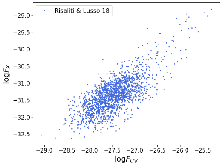
In this paper, we turn the improved “clean” sample including 1598 quasars, with reliable measurements of intrinsic X-ray and UV emissions assembled in Risaliti & Lusso (2018). The flux measurements concerning X-ray and UV emissions with the final sample is shown in Fig. 1. Possible cosmological application of these standard candles has recently been discussed in the literature (Melia, 2019). More recently, the multiple measurements of high-redshift quasars have been used for testing the cosmic distance duality relation (CDDR), based on the relation between the UV and X-ray luminosities of quasars, combined with the VLBI observations of compact structure in radio quasars (Zheng et al., 2020).

According to the Eq. (6), we would be able to derive luminosity distances $D_{L}(z)$ and hence dimensionless co-moving distances of the lens $d_{l}$ and the source $d_{s}$ for each SGL system, from UV and X-ray fluxes of the quasars whose redshifts are equal to $z_{l}$ and $z_{s}$, respectively. However, there are two potential problems to be solved. First is a high intrinsic scatter ($\hat{\delta}$) in the quasars sample, based on the UV and X-ray flux measurements. Second is that $\hat{\beta}$ and $\hat{\gamma}$ parameters are unknown. Fortunately, Melia (2019) used the quasars sample to achieve cosmological test without any external calibrator, treating the slope $\hat{\gamma}$, the intercept $\hat{\beta}$, and the intrinsic scatter $\hat{\delta}$ as free parameters to be fit. It was revealed that the quasar data can be self-calibrated under such individual optimization within a specified cosmology. For example in $\Lambda$CDM model one obtains: $\hat{\gamma}=0.639\pm 0.005$, $\hat{\beta}=7.02\pm 0.012$, $\hat{\delta}=0.231\pm 0.0004$, and $\Omega_{m}=0.31\pm 0.05$. In this analysis, we will not confine ourselves to any specific cosmology, but instead we reconstruct the dimensionless co-moving distance function $d(z)$, modeled as a polynomial expansion in $z$ or logarithmic polynomial expansion of $\log(1+z)$ (Räsänen et al., 2015; Liao et al., 2017a; Li et al., 2018). For the first case, the dimensionless angular diameter distance is parameterized by a third-order polynomial function of redshift

$$d(z)=z+a_{1}z^{2}+a_{2}z^{3},$$ (10)

with the initial conditions of $d(0)=0$ and $d^{{}^{\prime}}(0)=1$. For the second case, we perform empirical fit to the quasar measurements, based on a third-order logarithmic polynomial of

$$d(z)=ln(10)(x+b_{1}x^{2}+b_{2}x^{3}),$$ (11)

with $x=\log(1+z)$. Note that in the above two parameterizations, ($a_{1}$, $a_{2}$) and ($b_{1}$, $b_{2}$) represent two sets of constant parameters that need to be optimized and determined by flux measurements data in X-ray and UV emissions. Meanwhile, the logarithmic parametrization, benefiting from a more rapid convergence at high redshifts with respect to the standard linear parametrization, has proved to be a more reasonable approximation at high redshifts (Risaliti & Lusso, 2018).

Figure 3: Left panel: Fractional uncertainty of the velocity dispersion ($\Delta\sigma_{v}/\sigma_{v}$) as a function of the lens surface brightness ($B$) for the SLACS sample, with the best-fitted correlation function denoted as the red solid line. Right panel: The distribution of the velocity dispersion uncertainty for the simulated SGL sample.

Figure 4: The scatter plot of the simulated lensing systems based on the standard polynomial model (left panel) and logarithmic polynomial model (right panel), with the gradient color denoting the value of the Einstein radius.

In order to reconstruct the profile of dimensionless co-moving distance $d(z)$ function up to the redshifts $z=5.0$, we make use of the publicly available code called the emcee (Foreman et al., 2013), to obtain the best-fit values and the corresponding $1\sigma$ uncertainties of relevant parameters ($a_{1}$, $a_{2}$, $b_{1}$ and $b_{2}$ in our case). It is worth stressing here that one may worry that the cosmographic expansions are only valid at low redshift. However, the recent analysis of high-redshift Hubble diagram indicated that these relations are valid beyond $z\sim 4$, although fitting a log polynomial cosmography may hide certain features of the quasar data (Yang & Banerjee, 2019). Meanwhile, our results demonstrate that a third-order polynomial function adopted in Risaliti & Lusso (2018) is sufficient enough to expand the luminosity distance, since the inclusion of higher orders in the polynomial expansion have negligible effect on the final reconstruction results. The chi-square $\chi^{2}$ objective function we minimized is defined as

$$\chi^{2}=\sum_{i=1}^{1598}\frac{[\log(F_{X,i})-\Psi_{th}([F_{UV}]_{i};D_{L}[z_{i}])]^{2}}{\sigma_{F_{X,i}}^{2}+\hat{\delta}^{2}},$$ (12)

where $\hat{\delta}$ represents the global intrinsic dispersion, the $\sigma_{F_{X,i}}$ denotes the i-th measurement error of flux $F_{X,i}$ in X-ray waveband. The function $\Psi_{th}$ is defined as

$$\Psi_{th}=\hat{\beta}+\hat{\gamma}\log(F_{UV,i})+2(\hat{\gamma}-1)\log(D_{L}(z_{i})),$$ (13)

in terms of the measured fluxes ($F_{X,i}$, $F_{UV,i}$) and the luminosity distance $D_{L}(z)=c/H_{0}(1+z)d(z)$. It should be pointed out that the measurement error of the flux in UV band is ignored in this analysis since $\sigma_{F_{UV,i}}$ is insignificant comparing with $\sigma_{F_{X,i}}$ and $\hat{\delta}$. Meanwhile, we have also assumed a fiducial value for the Hubble constant $H_{0}=67.4$ km s^-1 Mpc^-1, based on the results obtained from Planck 2018 data (TT, TE, EE+lowE+lensing) (Aghanim et al., 2018). For the first case, the best-fit quasar parameters and the 68% C.L. are determined as $\hat{\gamma}=0.613\pm 0.011$, $\hat{\beta}=7.970\pm 0.312$, and $\hat{\delta}=0.230\pm 0.003$. The corresponding results will change to $\hat{\gamma}=0.616\pm 0.011$, $\hat{\beta}=7.530\pm 0.283$, and $\hat{\delta}=0.230\pm 0.003$ for the second case.

3.2 The simulated SGL data from LSST

It is broadly reckoned that the future wide-area and deep surveys, such as the Large Synoptic Survey Telescope (Verma et al., 2019) and the Dark Energy Survey (DES) (Frieman et al., 2004) will revolutionize the strong lensing science, by increasing the number of known galactic lenses by orders of magnitude. More specifically, the forthcoming photometric LSST survey will discover $\sim 10^{5}$ strong gravitational lenses (Collett, 2015), the cosmological application of which has become the focus of the forecasted yields of LSST in the near future (Cao et al., 2017c, 2018; Ma et al., 2019; Cao et al., 2020).

Based on the publicly available simulation programs explicitly described in Collett (2015), we simulate a realistic population of strong lensing systems with early-type galaxies acting as lenses. The singular isothermal sphere (SIS) is adopted to model the mass distributions of the lensing galaxies, the number density of which is characterized by the velocity dispersion function (VDF) from the measurements of SDSS Data Release 5 (Choi et al., 2007). Now one important issue should be emphasized in our simulations. In order to achieve our $\Omega_{k}$ test with the combination of strong lensing and stellar dynamics, valuable additional information such as spectroscopic redshifts ($z_{l}$ and $z_{s}$) and spectroscopic velocity dispersion ($\sigma_{ap}$) are necessary. Since these dedicated observations and substantial follow-up efforts for a sample of $10^{5}$ SGL systems are expensive, it is more realistic to focus only on a particular well-selected subset of LSST lenses, as was proposed in the recent discussion of multi-object and single-object spectroscopy to enhance Dark Energy Science from LSST (Hložek et al., 2019; Mandelbaum et al., 2019). Therefore, in our analysis the final SGL sample is restricted to 5000 elliptical galaxies with the velocity dispersion of 200 km/s $<\sigma_{ap}<$ 300 km/s, following the recent investigation of medium-mass lenses to minimize the possible discrepancy between Einstein mass and dynamical mass for the SIS model (Cao et al., 2016). The final simulated results show that the distributions of velocity dispersions and Einstein radii are very similar to those of the current SL2S sample (Sonnenfeld et al., 2013b).

Figure 5: Redshift distribution of quasars used to assess distances and SGL systems from future LSST survey.

Concerning the uncertainty budget, LSST could provide high-quality (sub-arcsecond) imaging data in general, especially in the $g$-band. However, in order to extract the full potential of LSST, obtaining high-resolution images for the lensing systems could also require additional imaging data from space-based facilities (HST), with detailed follow-up of individual SGL systems. Meanwhile, the participation of other ground-based facilities makes it possible to derive additional spectroscopic information, i.e., lens redshifts, source redshifts, and velocity dispersion measurements for individual lenses. In this analysis, different strategies will be applied to cope with the fractional uncertainty of the Einstein radius and stellar velocity dispersion, considering the possible correlations between the observational precision and other intrinsic properties of the lensing system (such as the mass or the brightness of the lens).

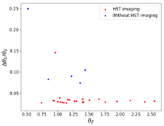
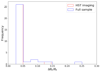
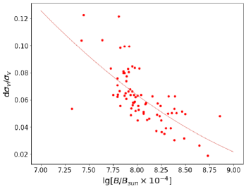
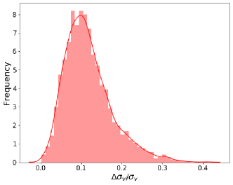
For the uncertainty of the Einstein radius, we turn to 32 SGL systems recently detected by Strong Lensing Legacy Survey (SL2S), with Canada CFrance CHawaii Telescope (CFHT) near-infrared ground-based images or Hubble Space Telescope (HST) imaging data (Sonnenfeld et al., 2013b). The HST imaging data were taken with the Advanced Camera for Surveys (ACS; filters: F814W/F606W; exposure time: 800/400s), Wide Field and Planetary Camera 2 (WFPC2; filter: F606W; exposure time: 1200s), and Wide Field Camera 3 (WFC3; filters: F600LP/F475X; exposure time: 720s), which have been observed with HST as part of programs 10876, 11289 (PI: J. P. Kneib) and 11588 (PI: R. Gavazzi). In addition to space-based photometry, the NIR images for some of the SL2S lenses were observed with the instrument WIRCam (Puget et al., 2004) in the $K_{s}$, $J$ and $H$ bands. We refer the reader to Sonnenfeld et al. (2013b) for more detailed information of the CFHT observations for each target (exposure time, etc.). The scatter and histogram plots of the fractional uncertainty of Einstein radius are respectively shown in Fig. 2, concerning the full sample with HST+CFHT imaging and the sub-sample with HST imaging. Not surprisingly, most of the lenses with high-precision Einstein radius measurements are derived from systems with HST data. Focusing on the full catalogue of SGL systems, one can clearly see a possible correlation between the fractional uncertainty of the Einstein radius and $\theta_{E}$, i.e. the lenses with smaller Einstein radii would suffer from large $\theta_{E}$ uncertainty, as reported previously in the previous strong lensing analysis. Meanwhile, for the full sample with HST+CFHT imaging data (i.e., CFHT image when HST image is not available), the fractional uncertainty of the Einstein radius is taken at the level of 8%, 5% and 3% (the mean uncertainty within each certain $\theta_{E}$ bin) for small Einstein radii lenses ($0.5"<\theta_{E}<1.0"$), intermediate Einstein radii lenses ($1"\leq\theta_{E}<1.5"$), and large Einstein radii lenses ($\theta_{E}\geq 1.5$). Such error strategy will be implemented in the simulations of our LSST lens sample. Meanwhile, in the optimistic case, i.e. when all of the LSST lenses considered in this work will be observed with HST-like image quality, it is reasonable to take the fractional uncertainty of the Einstein radius at a level of 3% (Hilbert et al., 2009). For the uncertainty of the velocity dispersion, we turn to 70 SGL systems observed in the Sloan Lens ACS survey (SLACS) (Bolton et al., 2008) and quantitatively analyze its correlation with the lens surface brightness in the $i$-band. The population of strong lenses is dominated by galaxies with velocity dispersion of $\sigma_{ap}\sim 230$ km/s (median value), while the Einstein radius distribution is characterized by the median value of $\theta_{E}=1.10"$. Such restricted SLACS lens sample, which falls within the velocity dispersion criterion applied in this analysis (200 km/s $<\sigma_{ap}<$ 300 km/s), is a good representative sample of what the future LSST survey might yield. As can be clearly seen from the results shown in Fig. 3, strong evidence of anti-correlation between these two quantities is revealed in our analysis. Using the best-fitted correlation function derived from the current SGL sample, we obtain in Fig. 3 the distribution of velocity dispersion uncertainty for the lenses discoverable in forthcoming LSST survey, which is well consistent with the previous strategy of assigning an overall error of 5% on $\sigma_{ap}$ (Cao et al., 2015b; Zhou & Li, 2020).

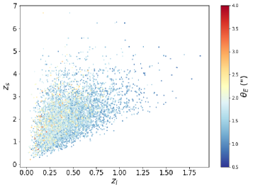
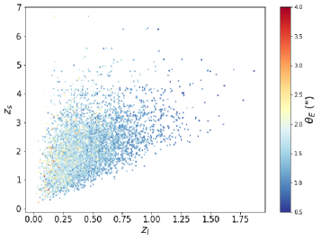
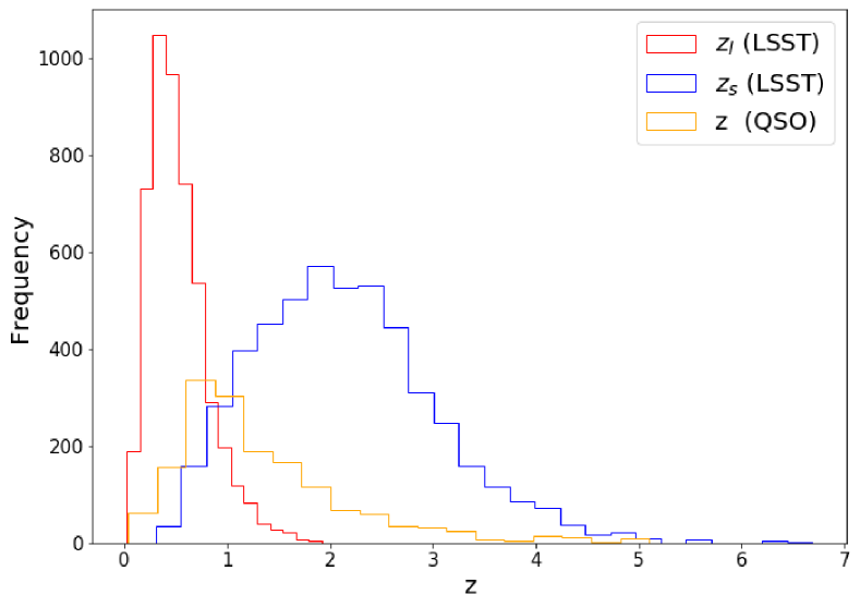
It should be pointed out that LSST will discover a number of fainter, smaller-separation lenses where it is not clear that the same level of precision can be reached. Therefore, two selection criteria of the Einstein radius and the $i$-band magnitude are applied to our particular well-selected subset of LSST lenses ($\theta_{E}>0.5"$ and $m_{i}<22$). In this paper, we generate two SGL samples using the standard polynomial and logarithmic polynomial cosmographic reconstructions (taking the best fitted parameters of these reconstructions). The scatter plots of the simulated lensing systems based on standard polynomial and logarithmic polynomial cosmographic reconstructions are shown in Fig. 4. For a good comparison, Fig. 5 illustrates the redshift coverage of the current quasar sample and simulated SGL sample, which demonstrates the perfect consistency between the redshift range of high-$z$ quasars and LSST lensing systems.

Standard polynomial	$\Omega_{k}$	$f_{E}$	$\gamma$	$\alpha$	$\delta$
SIS	$0.002\pm 0.035$	$1.000\pm 0.002$	$\Box$	$\Box$	$\Box$
Power-law spherical	$-0.007\pm 0.029$	$\Box$	$2.000\pm 0.012$	$\Box$	$\Box$
Extended power-law	$0.003\pm 0.045$	$\Box$	$\Box$	$2.000\pm 0.014$	$2.171\pm 0.035$
Power-law spherical (with HST imaging)	$-0.008\pm 0.028$	$\Box$	$2.000\pm 0.012$	$\Box$	$\Box$
logarithmic polynomial	$\Omega_{k}$	$f_{E}$	$\gamma$	$\alpha$	$\delta$
SIS	$-0.001\pm 0.030$	$1.000\pm 0.003$	$\Box$	$\Box$	$\Box$
Power-law spherical	$-0.007\pm 0.016$	$\Box$	$2.000\pm 0.013$	$\Box$	$\Box$
Extended power-law	$0.002\pm 0.031$	$\Box$	$\Box$	$2.002\pm 0.016$	$2.172\pm 0.035$

Table 1: Constraints on the cosmic curvature and lens profile parameters for three types of lens models, in the framework of standard polynomial and logarithmic polynomial cosmographic reconstructions.

4 Results and discussion

The constraints on the cosmic curvature, based on the simulated SGL systems supplemented with the constructed Hubble diagram of high-redshift quasars, are obtained by maximizing the likelihood ${\cal L}\sim\exp{(-\chi^{2}/2)}$. In our analysis, $\chi^{2}$ is constructed as

$$\chi^{2}(\textbf{p},\Omega_{k})=\sum_{i=1}^{N}\frac{\left({\cal D}_{th}({z}_{i};\Omega_{k})-{\cal D}_{obs}({z}_{i};\textbf{p})\right)^{2}}{\sigma_{\cal D}(z_{i})^{2}},$$ (14)

where ${\cal D}=d_{ls}/d_{s}$ and $N$ is the number of the data points. The theoretical distance ratio $\mathcal{D}_{th}$ dependent on $\Omega_{k}$ is given by Eq. (4), while its observational counterpart is dependent on the lens model adopted Eq. (5), (6) and (7). Free parameters in these lens model are collectively denoted as p, and $\sigma_{D}$ stands for the uncertainty of the distance ratio expressed as $\sigma_{D}^{2}=\sigma_{SGL}^{2}+\sigma_{QSO}^{2}$. Note that the statistical error of SGL ($\sigma_{SGL}$) is propagated from the measurement uncertainties of the Einstein radius and velocity dispersion, while $\sigma_{QSO}$ depends on the uncertainties of $d(z)$ function (polynomial and log-ploynomial parameterized distance) reconstructed from the quasars. As previously mentioned, the aim of this work is to estimate the cosmic curvature by combining the constructed Hubble diagram of high-redshift quasars with galactic-scale strong lensing systems expected to be seen by the forthcoming LSST survey. Therefore, our analysis will be performed on two different reconstruction schemes: the standard polynomial cosmographic reconstruction and the logarithmic polynomial reconstruction. The numerical results for the cosmic curvature $\Omega_{k}$ and lens model parameters are summarized in Table 1, with the marginalized distributions with 1$\sigma$ and 2$\sigma$ contours shown in Fig. 7.

Figure 6: The 2-D regions and 1-D marginalized distribution with the 1-$\sigma$ and 2-$\sigma$ contours of all parameters from the standard polynomial (blue dotted line) and the logarithmic polynomial (green solid line) cosmographic reconstruction, in the framework of three lens models: SIS (left), power-law profile (middle), and extended power-law profile (right), respectively.

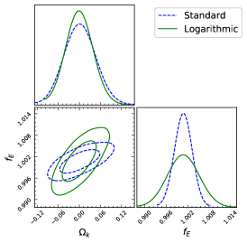
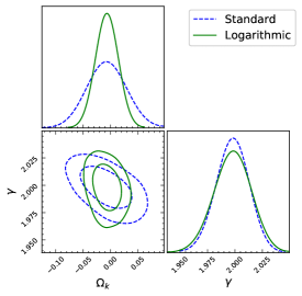
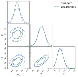
Let us start our analysis with the standard polynomial cosmographic reconstruction and consider three lens mass density profiles: SIS, power-law model, and extended power-law model. For the simplest SIS model, the numerical and graphical results are respectively presented in Table 1 and Fig. 7, with the best-fitted values for the parameters: $\Omega_{k}=0.002\pm 0.035$ and $f_{E}=1.000\pm 0.002$. On the one hand, one may clearly see the degeneracy between the cosmic curvature and the lens model parameters, a tendency revealed and extensively studied in the previous works (Zhou & Li, 2020). The best-fitted value of $f_{E}$ is exactly what one could expect knowing how the SGL data were simulated, i.e. the SIS velocity dispersion is equal (up to some noise added) to the observed velocity dispersion reported in mock catalog. This supports reliability of our procedure. On the other hand, a spatially flat universe is supported at much higher confidence levels ($\Delta\Omega_{k}\sim 10^{-2}$), compared with the previous results obtained in Xia et al. (2017); Qi et al. (2019a) by applying the above procedure to different available SGL subsamples. In the framework of power-law mass density profile, one can derive constraint on the cosmic curvature as $\Omega_{k}=-0.007\pm 0.029$, with the best-fitted lens parameter and the corresponding 1$\sigma$ uncertainty: $\gamma=2.000\pm 0.012$. In addition, it is worth noting that when the fractional uncertainty of the Einstein radius is reduced to the level of 3% (with HST imaging), the resulting constraint on the cosmic curvature becomes $\Delta\Omega_{k}=0.028$. Therefore, the estimation of the spatial curvature is more sensitive to the measurements of lens velocity dispersions, which indicates the importance of deriving additional spectroscopic information for individual lenses. In the case of extended power-law lens model, we get the weakest fits on the cosmic curvature in the three types of lens models, with the best-fit value and the marginalized 1$\sigma$ uncertainty $\Omega_{k}=0.003\pm 0.045$. Whereas, our analysis also yield improved constraints on the the total-density and luminosity density profiles, $\alpha=2.000\pm 0.014$ and $\delta=2.171\pm 0.035$. Compared with the profile of the total mass, the density of luminous baryoic mass has exhibited slight different distribution in early-type galaxies, i.e, the stellar mass profile in the inner region of massive lensing galaxies could fall off steeply than that of the total mass. Such tendency, which has been revealed and studied in detail in Cao et al. (2016), might helpfully contribute to the understanding of the presence of dark matter, which is differently spatially extended than luminous baryons in early-type galaxies. More importantly, besides the different degree of degeneracy between the lens model parameters, our analysis also reveals the strong correlation between $\Omega_{k}$ and the parameters characterizing the lens mass profiles. Therefore, the large covariances of $\Omega_{k}$ with the power-law parameters seen in Fig. 6 motivates the future use of auxiliary data to improve constraints on the galaxy structure parameters. Now, the question is: What is the average $\alpha$, $\delta$ and their intrinsic scatter for the overall population of early-type galaxies? One can use high-cadence, high-resolution and multi-filter imaging of the resolved lensed images, to put accurate constrains on the density profiles of galaxies (Suyu et al., 2006; Vegetti et al., 2010; Collett & Auger, 2014; Wong et al., 2015), with the newly developed state-of-the-art lens modeling techniques and kinematic modeling methods (Suyu et al., 2012). More specifically, the joint lensing and dynamical studies of the SL2S lens sample have demonstrated that the precision of 5% could be obtained for the total-mass density slope inside the Einstein radius (Ruff et al., 2011; Sonnenfeld et al., 2013b) Hence, the LSST lenses should be technically supported by dedicated follow-up imaging of the lensed images, possibly performed with more frequent visits on Hubble telescope and smaller ground-based telescopes. Meanwhile, observations of the lens galaxy spectra are also needed in order to obtain the kinematic velocity dispersions, which could be satisfied by Adaptive optics (AO) IFU spectroscopy on 8-40m-class telescopes. Other possible solutions to this issue can simultaneously satisfy all of these needs, focusing on the combination of AO imaging with slit spectroscopy (Hložek et al., 2019).

Another important issue is the choice of the $D_{L}(z)$ function reconstructed from current quasar sample that served for the $\Omega_{k}$ estimation. Therefore, we perform a similar analysis with the logarithmic polynomial reconstruction and obtained the constraints in the parameter space of $\Omega_{k}$ and ($f_{E},\gamma,\alpha,\delta$) for three cases of mass density profiles. The results are also shown in Fig. 6 and Table 1. Comparing constraints based on the two different reconstructions, we see that confidence regions of different parameters (cosmic curvature and lens model parameters) are well overlapped with each other; hence our results and discussions presented above are robust. The strong degeneracies between the cosmic curvature parameter and the lens model parameters are also present as illustrated in Fig. 8. More interestingly, compared with the standard polynomial reconstruction, the advantage of the logarithmic polynomial reconstruction is that it could provide more stringent constraints on the cosmic curvature: $\Omega_{k}=-0.001\pm 0.030$, $\Omega_{k}=-0.007\pm 0.016$ and $\Omega_{k}=0.002\pm 0.031$, respectively in the framework of three lens mass density profiles (SIS model, power-law spherical model, and extended power-law model). Our results indicate that logarithmic parametrization is a more reasonable approximation of theoretical values up to high redshift. Such findings, which highlight the importance of choosing a reliable $D_{L}(z)$ parametrization to better investigate the spatial properties in the early universe, have also been noted and discussed in the previous works (Risaliti & Lusso, 2018; Melia, 2019). It should be noted that, even though we focus on the simulated data of SGL systems trying to assess the performance of the method in the future, the reconstructed distances are obtained from the real data. Hence, the best-fitted values of $\Omega_{k}$ somehow reflect what is supported by the observational data.

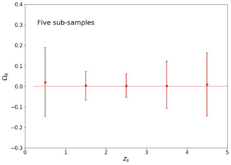
Finally, an accurate reconstruction of cosmic curvature with redshift can greatly contribute to our understanding of the inflation models and fundamental physics. In order to address this issue, we divide the full SGL sample into five groups with $\Delta z_{s}=1.0$ (based on the source redshifts) and obtain the constraints on $\Omega_{k}$ in the framework of SIS model. The first subsample has 400 SGL with source redshifts $z_{s}<1.0$, the second subsample has 2000 SGL with $1.0<z_{s}<2.0$, the third subsample has 1800 SGL with $2.0<z_{s}<3.0$, the fourth subsample has 600 SGL with $3.0<z_{s}<4.0$, and the fifth subsample contains 200 SGL with source redshifts $4.0<z_{s}<5.0$. The corresponding results are shown in Fig. 7, with the $d(z)$ function (polynomial and log-ploynomial parameterized distance) reconstructed from the full quasar sample. Compared with the previous analysis performed to test cosmic curvature with different tests involving other popular astrophysical probes including SNe Ia (Xia et al., 2017) and compact radio quasars (Qi et al., 2019a), it is suggested that our technique, i.e., using luminosity distance of quasars directly derived from the non-linear relation between X-ray and UV luminosities, will considerably improve such direct measurement of the spatial curvature in the early universe ($z\sim 5.0$).

Figure 7: Determination of cosmic curvature with five subsamples $0<z<1.0$, $1.0<z<2.0$, $2.0<z<3.0$, $3.0<z<4.0$ and $4.0<z<5.0$ based on the source redshifts of SGL sample characterized by the SIS lens model.

5 Conclusions

In this paper, we re-estimate which precision can be achieved for the cosmic curvature in the near future, on the basis of the distance sum rule in the well-known FLRW metric (Räsänen et al., 2015). For the purpose, we focus on the simulated data of SGL systems expected to be detected by LSST, combined with the recently assembled catalog of 1598 high-quality quasars calibrated as standard candles. It is demonstrated that in the framework of such cosmological-model-independent way, the quasars have better coverage of redshift in SGL systems at high redshifts, which makes it possible to study the spatial properties in the early universe. Our main conclusions are summarized as follows:

• Based on the future measurements of a particular well-selected subset of 5000 LSST lenses (with source redshifts $z\sim 5.0$), the final results show that the the cosmic curvature could be estimated with the precision of $\Delta\Omega_{k}\sim 10^{-2}$, which is comparable to that derived from the Planck CMB power spectra (TT, TE, EE+lowP) (Aghanim et al., 2018). It should be pointed out, even though the simulated data of SGL systems are used in our analysis , the reconstructed distances are obtained from the currently compiled quasar sample. In particular, no assumption on the cosmic curvature is made the simulation of the LSST lens sample, i.e., two SGL samples using the standard polynomial and logarithmic polynomial cosmographic reconstructions. Therefore, the best-fitted values of $\Omega_{k}$ somehow reflect what is supported by the real observational data.

• In our analysis, three types of models, which has been extensively investigated in the literature is considered to describe the structure of the lens. Specially, one may obtain the most stringent fits on the cosmic curvature in the power-law lens model, while our $\Omega_{k}$ estimation will be strongly affected by the complicated extended power law model (considering the possible difference between the luminosity density profile ($\nu(r)\sim r^{-\delta}$) and the total-mass). Furthermore, our analysis also reveals the strong correlation between the cosmic curvature ($\Omega_{k}$) and parameters characterizing the mass profile of lens galaxies ($f_{E}$, $\gamma$, and $\alpha$, $\delta$), which motivates the future investigation of lens density profiles through the combination of state-of-the-art lens modeling techniques and kinematic modeling methods (Suyu et al., 2012). There are several sources of systematics that remain to be discussed and addressed in the future analysis. The first one is related to the galaxy structure parameters, especially those characterizing the stellar distribution in the lensing galaxies. In this paper, we adopted a power-law profile in the spherical Jeans equation, with the aim of connecting the observed velocity dispersion to the dynamical mass. However, many modern lens models have considered a two-component model that is the sum of a Sersic-like profile (fit to the stellar light distribution) and a NFW profile (fit to the dark matter distribution) (Navarro, Frenk & White, 1997). The luminosity distribution of spherical galaxies could also be well described by the well-known Hernquist profile, whose behavior follows an inner slope of $r^{-1}$ at small radii and $r^{-4}$ at large radii (Hernquist et al., 1990). Enlightened by the most recent studies trying to quantify how cosmological constraints are altered by different luminosity density profiles (Ma et al., 2019), such effect will contribute to the scatter in our cosmic-curvature test. This also highlights the importance of auxiliary data in improving constraints on the luminosity density profile, i.e., more high-quality integral field unit (IFU) data are needed to further improve the method in view of upcoming surveys (Barnabè et al., 2013).

• Our results indicate that, properly calibrated UV - X-ray relation in quasars has a great potential of becoming an important and precise distance estimator in cosmology. Based on the two cosmographic reconstructions of $D_{L}(z)$ function, our findings also highlight the importance of choosing a reliable reconstruction schemes in order to better investigate the nature of space-time geometry at high redshifts. This conclusion is also confirmed by the the reconstruction of cosmic curvature with the source redshift $z_{s}$, with accurate observations and spectral characterization of quasars observed by SDSS (Shen et al., 2011; Paris et al., 2017) and XMM (Rosen et al., 2016). Finally, this paper seeks to highlights the potential of LSST, which is expected to find extraordinary numbers of new transients every night (Smith et al., 2019). For instance, one should recall that other promising settings for SGL systems have been proposed, for example, galactic-scale strong gravitational lensing systems with Type Ia supernovae (Goobar et al., 2017; Cao et al., 2018, 2019c) and gravitational waves (GWs) as background sources (Liao et al., 2017b; Cao et al., 2019a; Qi et al., 2019b, c). Benefit from LSST’s wide-field of view and sensitivity, these upcoming improvements on the precision of cosmic curvature estimation will be very helpful for revealing the physical mechanism of cosmic acceleration, or the nature of cosmic origins.

References

- Aghanim et al. (2018) Aghanim, N., Akrami, Y., Ashdown, M., et al. Planck Collaboration, 2018, arXiv:1807.06209
- Avni & Tananbaum (1986) Avni, Y., & Tananbaum, H. 1986, ApJ, 305, 83
- Baldwin (1977) Baldwin, J. A. 1977, ApJ, 214, 679
- Barnabè et al. (2013) Barnabè, M., et al. 2013, MNRAS, 436, 253
- Bernstein (2006) Bernstein, G. 2006, ApJ, 637, 598
- Bisogni et al. (2018) Bisogni, S., Risaliti, G. & Lusso, E. 2018, Front. Astron. Space Sci. 4:68; [doi: 10.3389/fspas.2017.00068 ]
- Bolton et al. (2012) Bolton, A. S., et al. 2012, ApJ, 757, 82
- Bolton et al. (2008) Bolton, A. S., et al. 2008, ApJ, 682, 964
- Cai et al. (2016) Cai, R., Guo, Z., & Yang, T. 2016, PRD, 93, 043517
- Cao et al. (2011) Cao, S., Zhu, Z.-H., & Zhao, R. 2011, PRD, 84, 023005
- Cao & Zhu (2012) Cao, S., & Zhu, Z.-H. 2012, A&A, 538, A43
- Cao, Covone & Zhu (2012) Cao, S., Covone, G., & Zhu, Z.-H. 2012, ApJ, 755, 31
- Cao et al. (2012) Cao, S., Pan, Y., Biesiada, M., Godlowski, W., & Zhu Z.-H. 2012, JCAP, 03, 016
- Cao et al. (2013) Cao, S., et al. 2013, RAA, 13, 15
- Cao et al. (2015a) Cao, S., et al. 2015a, AJ, 149, 3
- Cao et al. (2015b) Cao, S., Biesiada, M., Gavazzi, R., Piórkowska, A., & Zhu, Z.-H. 2015b, ApJ, 806, 185
- Cao et al. (2016) Cao, S., Biesiada, M., Yao, M., & Zhu, Z.-H. 2016, MNRAS, 461, 2192
- Cao et al. (2017a) Cao, S., et al. 2017, JCAP, 02, 012
- Cao et al. (2017b) Cao, S., et al. 2017, A&A, 606, A15
- Cao et al. (2017c) Cao, S., et al. 2017, ApJ, 835, 92
- Cao et al. (2018) Cao, S., et al. 2018, ApJ, 867, 50
- Cao et al. (2019a) Cao, S., et al. 2019, NatSR, 9, 11608
- Cao et al. (2019b) Cao, S., et al. 2019, PDU, 24, 100274
- Cao et al. (2019c) Cao, S., et al. 2019, PRD, 100, 023530
- Cao et al. (2020) Cao, S., et al. 2020, ApJL, 888, L25
- Chen et al. (2019) Chen, Y., Li, R., Shu, Y. & Cao, X. 2019, MNRAS, 488, 3745
- Choi et al. (2007) Choi, Y.-Y., Park, C., & Vogeley, M. S. 2007, ApJ, 884, 897
- Clarkson et al. (2007) Clarkson, C., Cortes, M., & Bassett, B. 2007, JCAP. 08, 011
- Clarkson et al. (2008) Clarkson, C., Bassett, B., Lu, T. H.-C. 2008, PRL, 101, 011301
- Collett & Auger (2014) Collett, T. E. & Auger, M. W. 2014, MNRAS, 443, 969
- Collett (2015) Collett, T. E. 2015, ApJ, 811, 20
- Collett et al. (2018) Collett, T. E., et al. 2018, Science, 360, 1342
- Denissenya et al. (2018) Denissenya, M., Linder, E. V., & Shafieloo, A. 2018, JCAP, 03, 041
- Foreman et al. (2013) Foreman-Mackey, D., Hogg, D. W., Lang, D.& Goodman, J. 2013, PASP, 125, 306
- Frieman et al. (2004) Frieman, J., & Dark Energy Survey Collaboration, 2004, BAAS, 36, 1462
- Futamase & Yoshida (2001) Futamase, T., & Yoshida, S. 2001, PThPh, 105, 887
- Gerhard et al. (2001) Gerhard, O., et al. 2001, AJ, 121, 1936
- Gong & Wang (2007) Gong, Y.-G., & Wang, A. 2007, PRD, 75, 043520
- Goobar et al. (2017) Goobar, A., et al. 2017, Science, 356, 291
- Hernquist et al. (1990) Hernquist, L. 1990, ApJ, 356, 359
- Hilbert et al. (2009) Hilbert, S., et al. 2009, A&A, 499, 31
- Hložek et al. (2019) Hložek, R. A., et al. arXiv:1903.09324
- Holanda et al. (2017) Holanda, R. F. L., et al. 2017, MNRAS 471, 3079
- Humphrey & Buote (2010) Humphrey, P. J., & Buote, D. A. 2010, MNRAS, 403, 2143
- Ichikawa et al. (2006) Ichikawa, K., et al. 2006, JCAP, 12, 005
- Koopmans et al. (2005) Koopmans, L. V. E. 2005, Proceedings of XXIst IAP Colloquium, (Paris, 4-9 July 2005), eds G. A. Mamon, F. Combes, C. Deffayet, B. Fort (Paris: EDP Sciences) [arXiv:0511121]
- Koopmans et al. (2006) Koopmans, L. V. E., et al. 2006, ApJ, 649, 599
- Li et al. (2016) Li, X. L., et al. 2016, RAA, 16, 84
- Li et al. (2016) Li, Z.-X., Wang, G.-J., Liao, K., & Zhu, Z.-H. 2016, ApJ, 833, 240
- Li et al. (2018) Li, Z.-X., Ding, X.-H., Wang, G.-J., Liao, K., & Zhu, Z.-H. 2018, ApJ, 854, 146
- Liao et al. (2017a) Liao, K., Li Z., Wang G.-J., Fan X.-L. 2017, ApJ, 839, 70
- Liao et al. (2017b) Liao, K., et al. 2017, Nature Communications, 8, 1148
- Liu et al. (2019) Liu, T. H., et al. 2019, ApJ, 886, 94
- Lusso et al. (2010) Lusso, E., et al. 2010, A&A, 512, 34
- Lusso & Risaliti (2016) Lusso, E., & Risaliti, G. 2016, ApJ, 819, 154
- Ma et al. (2019) Ma, Y. B., et al. 2019, EPJC, 79, 121
- Mandelbaum et al. (2019) Mandelbaum, R., et al. arXiv:1903.09323
- Melia (2019) Melia, F. 2019, MNRAS, 489, 517
- Navarro, Frenk & White (1997) Navarro, J. F, Frenk, C. S, & White, S. D. M. 1997, ApJ, 490, 493
- Ofek et al. (2003) Ofek, E. O., Rix, H. W., & Maoz, D. 2003, MNRAS, 343, 639
- Oguri & Marshall (2010) Oguri, M., & Marshall, P. J. 2010, MNRAS, 405, 2579
- Ooba & Sugiyama (2018) Ooba, J., Ratra, B., & Sugiyama, N. 2018, ApJ, 864, 80
- Paris et al. (2017) Paris, I., et al. 2017, A&A, 597, 79
- Puget et al. (2004) Puget, P., Stadler, E., Doyon, R., et al. 2004, Proc. SPIE, 5492, 978
- Qi et al. (2019a) Qi, J.-Z., et al. 2019a, MNRAS, 483, 1
- Qi et al. (2019b) Qi, J. Z., et al. 2019b, PRD, 99, 063507
- Qi et al. (2019c) Qi, J. Z., et al. 2019c, PDU, 26, 100338
- Rana et al. (2017) Rana, A., Jain, D., Mahajan, S., & Mukherjee A. 2017, JCAP, 03, 028
- Räsänen et al. (2014) Rsnen, S., et al. 2014, JCAP, 03, 035
- Räsänen et al. (2015) Rsnen, S.,Bolejko, K., & Finoguenov, A. 2015, PRL, 115, 101301
- Rosen et al. (2016) Rosen, S. R., et al. 2016, A&A, 590, 1
- Risaliti & Lusso (2015) Risaliti, G., & Lusso, E. 2015, ApJ, 815, 33
- Risaliti & Lusso (2018) Risaliti, G., & Lusso, E. 2019, Nature Astronomy, 3, 272
- Ruff et al. (2011) Ruff, A. J., et al. 2011, ApJ, 727, 96
- Schwab et al. (2009) Schwab, J., Bolton, A. S., & Rappaport, S. A. 2009, ApJ, 708, 750
- Shafieloo & Clarkson (2010) Shafieloo, A., & Clarkson, C. 2010, PRD, 81, 083537
- Shen et al. (2011) Shen, Y., et al. 2011, ApJS, 194, 45
- Smith et al. (2019) Smith, G. P., et al. arXiv:1902.05140
- Sonnenfeld et al. (2013a) Sonnenfeld, A., et al. 2013a, ApJ, 777, 98
- Sonnenfeld et al. (2013b) Sonnenfeld, A., Gavazzi, R., Suyu, S. H., Treu, T., & Marshall, P. J. 2013b, ApJ, 777, 97
- Suyu et al. (2006) Suyu, S. H., et al. 2007 AAS/AAPT Joint Meeting, American Astronomical Society Meeting 209, id.21.02; Bulletin of the American Astronomical Society, Vol. 38, p.927
- Suyu et al. (2012) Suyu, S. H., et al. 2012, ApJ, 750, 10
- Suzuki et al. (2012) Suzuki, N. et al. (Supernova Cosmology Project), 2012, ApJ, 746, 85
- Takada & Doré (2015) Takada, M., & Doré, O., 2015, PRD, 92, 123518
- Vegetti et al. (2010) Vegetti, S., Koopmans, L. V. E., Bolton, A., Treu, T., & Gavazzi, R. 2010, MNRAS, 408, 1969
- Verma et al. (2019) Verma, A., et al. 2019, arXiv:1902.05141
- Virey et al. (2008) Virey, J. M., et al. 2008, JCAP, 12, 008
- Wang et al. (2013) Wang, J.-M., et al. 2013, PRL, 110, 081301
- Wang et al. (2017) Wang, G.-J., et al. 2017, ApJ, 847, 45
- Watson et al. (2011) Watson, D., et al. 2011, ApJL, 740, L49
- Wei & Wu (2017) Wei, J.-J., & Wu, X.-F. 2017, ApJ, 838, 160
- Wong et al. (2015) Wong, K. C., Suyu, S. H., & Matsushita, S. 2015, ApJ, 811, 115
- Wucknitz et al. (2004) Wucknitz, O., Biggs, A. D, Browne, I. W. A. 2004, MNRAS, 349, 14
- Xia et al. (2017) Xia, J.-Q., et al. 2017, ApJ, 834, 75
- Yang & Banerjee (2019) Yang, T., Banerjee, A., Colgáin, E. Ó. 2019, arXiv:1911.01681
- Young et al. (2010) Young, M., Risaliti, G. & Elvis, M. 2010, ApJ, 708, 1388
- Zheng et al. (2020) Zheng, X. G., et al. 2020, ApJ, 892, 103
- Zhou & Li (2020) Zhou, H. & Li, Z. 2020, ApJ, 899, 186