Uncertainty-Aware Blind Image Quality Assessment in the Laboratory and Wild

Abstract

Performance of blind image quality assessment (BIQA) models has been significantly boosted by end-to-end optimization of feature engineering and quality regression. Nevertheless, due to the distributional shift between images simulated in the laboratory and captured in the wild, models trained on databases with synthetic distortions remain particularly weak at handling realistic distortions (and vice versa). To confront the cross-distortion-scenario challenge, we develop a unified BIQA model and an approach of training it for both synthetic and realistic distortions. We first sample pairs of images from individual IQA databases, and compute a probability that the first image of each pair is of higher quality. We then employ the fidelity loss to optimize a deep neural network for BIQA over a large number of such image pairs. We also explicitly enforce a hinge constraint to regularize uncertainty estimation during optimization. Extensive experiments on six IQA databases show the promise of the learned method in blindly assessing image quality in the laboratory and wild. In addition, we demonstrate the universality of the proposed training strategy by using it to improve existing BIQA models.

I Introduction

With the inelastic demand for processing massive Internet images, it is of paramount importance to develop computational image quality models to monitor, maintain, and enhance the perceived quality of the output images of various image processing systems [1]. High degrees of consistency between model predictions and human opinions of image quality have been achieved in the full-reference regime, where distorted images are compared to their reference images of pristine quality [2]. When such information is not available, no-reference or blind image quality assessment (BIQA) that relies solely on distorted images becomes more practical yet more challenging. Recently, deep learning-based BIQA models have experienced an impressive series of successes due to joint optimization of feature representation and quality prediction. However, these models remain particularly weak at cross-distortion-scenario generalization [3]. That is, models trained on images simulated in the laboratory cannot deal with images captured in the wild. Similarly, models optimized for realistic distortions (e.g., sensor noise and poor exposure) do not work well for synthetic distortions (e.g., Gaussian blur and JPEG compression).

(a)

(b)

(c)

(d)

(e)

(f)

Figure 1: Images with approximately the same linearly re-scaled MOS exhibit drastically different perceptual quality. If the human scores are in the form of DMOSs, we first negate the values followed by linear re-scaling. These are sampled from (a) LIVE [4], (b) CSIQ [5], (c) KADID-10K [6], (d) BID [7], (e) LIVE Challenge [8], and (f) KonIQ-10K [9]. It is not hard to observe that image (f) has clearly superior quality than the other five. All images are cropped for better visibility.

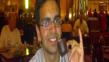
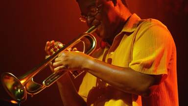
A seemingly straightforward method of adapting to the distributional shift between synthetic and realistic distortions is to directly combine multiple IQA databases for training. However, existing databases have different perceptual scales due to differences in subjective testing methodologies. For example, the CSIQ database [5] used a multiple stimuli absolute category rating in a well-controlled laboratory environment, with difference mean opinion scores (DMOSs) in the range of $[0,1]$, whereas the LIVE Challenge Database used a single stimulus continuous quality rating in an unconstrained crowdsourcing platform, with MOSs in the range of $[0,100]$. This means that a separate subjective experiment on images sampled from each database is required for perceptual scale realignment [4, 5]. To make this point more explicit, we linearly re-scaled the subjective scores of each of six databases [4, 5, 6, 7, 8, 9] to $[0,100]$, with a larger value indicating higher quality. Fig. 1 shows the sample images that have approximately the same re-scaled MOS. As expected, they appear to have drastically different perceptual quality. A more promising design methodology for unified BIQA is to build a prior probability model for natural undistorted images as the reference distribution, to which a test distribution of the distorted image can be compared. The award-winning BIQA model - NIQE [10] is a specific instantiation of this idea, but is only capable of handling a small number of synthetic distortions.

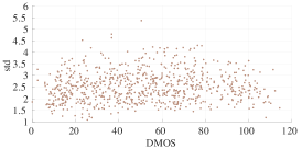
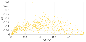
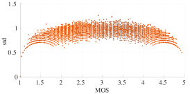
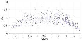
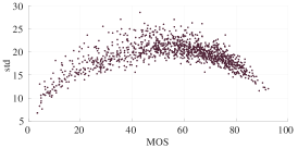
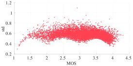
In addition to training BIQA models with (D)MOSs, there is another type of supervisory signal - the variance of human opinions, which we believe is beneficial for BIQA, but has not been fully explored. Generally, humans tend to give more consistent ratings (i.e., smaller variances) to images at the two ends of the quality range, while assessing images in the mid-quality range with less certainty (see Fig. 3). Therefore, it is reasonable to assume image quality models to behave similarly. Moreover, previous BIQA methods [11] have enjoyed the benefits of modeling the uncertainty of quality prediction for subsequent applications.

In this paper, we take steps toward developing unified uncertainty-aware BIQA models for both synthetic and realistic distortions. Our contributions include:

• A training strategy that allows differentiable BIQA models to be trained on multiple IQA database (of different distortion scenarios) simultaneously. In particular, we first sample and combine pairs of images within each database. For each pair, we leverage the human-rated (D)MOSs and variances to compute a probability value that one image is of better perceptual quality as the supervisory signal. The resulting training set bypasses additional subjective testing for perceptual scale realignment. We then use a pairwise learning-to-rank algorithm with the fidelity loss [12] to drive the learning of computational models for BIQA.

• A regularizer that enforces a hinge constraint on the learned uncertainty using the variance of human opinions as guidance. This enables BIQA models to mimic the uncertain aspects of humans when performing the quality assessment task.

• A Unified No-reference Image Quality and Uncertainty Evaluator (UNIQUE) based on a deep neural network (DNN) that performs favorably against state-of-the-art BIQA models on six IQA databases (see Table I) covering both synthetic and realistic distortions. We also verify its generalizability in a challenging cross-database setting and via the group maximum differentiation (gMAD) competition [13].

TABLE I: Comparison of human-rated IQA databases. MOS stands for mean opinion score. DMOS is inversely proportional to MOS

Database	# of Images	Scenario	Annotation	Range	Subjective Testing Methodology
LIVE [4]	779	Synthetic	DMOS, Variance	$[0,100]$	Single stimulus continuous quality rating
CSIQ [5]	866	Synthetic	DMOS, Variance	$[0,1]$	Multi stimulus absolute category rating
KADID-10K [6]	10,125	Synthetic	MOS, Variance	$[1,5]$	Double stimulus absolute category rating with crowdsourcing
BID [7]	586	Realistic	MOS, Variance	$[0,5]$	Single stimulus continuous quality rating
LIVE Challenge [8]	1,162	Realistic	MOS, Variance	$[0,100]$	Single stimulus continuous quality rating with crowdsourcing
KonIQ-10K [9]	10,073	Realistic	MOS, Variance	$[1,5]$	Single stimulus absolute category rating with crowdsourcing

TABLE II: Summary of ranking-based BIQA models. DS: distortion specification characterized by distortion parameters. FR: full-reference IQA model predictions

Model	RankIQA [14]	DB-CNN [3]	dipIQ [15]	Ma19 [16]	Gao15 [17]	UNIQUE
Source	DS	DS	FR	FR	(D)MOS	(D)MOS+Variance
Scenario	Synthetic	Synthetic	Synthetic	Synthetic	Synthetic	Synthetic+Realistic
Annotation	Binary	Categorical	Binary	Binary	Binary	Continuous
Loss Function	Hinge variant	Cross entropy	Cross entropy	Cross entropy variant	Hinge	Fidelity+Hinge
Ranking Stage	Pre-training	Pre-training	Prediction	Prediction	Prediction	Prediction

II Related Work

In this section, we give a review of existing BIQA models over the last two decades.

II-A BIQA as Regression

Early attempts at BIQA were tailored to specific synthetic distortions [18], such as JPEG compression [19] and JPEG2000 compression [20]. Later models aimed for general-purpose BIQA [21, 22, 23, 24, 25], with the underlying assumption that statistics extracted from natural images are highly regular [26] and distortions will break such statistical regularities. Based on natural scene statistics (NSS), a quality prediction function can be learned using standard supervised learning tools. Of particular interest is NIQE [10], which is arguably the first unified BIQA model with the goal of capturing arbitrary distortions. However, the NSS model used in NIQE is not sensitive to image “unnaturalness” introduced by realistic distortions [10]. Zhang et al. [27] extended NIQE [10] by exploiting a more powerful set of NSS for local quality prediction. However, the generalization to realistic distortions is still limited.

Joint optimization of feature engineering and quality regression enabled by deep learning has significantly advanced the field of BIQA in recent years. The apparent conflict between the small number of subjective ratings and the large number of learnable model parameters may be alleviated in three ways. The first method is transfer learning [28], which directly fine-tunes pre-trained DNNs for object recognition. Recently, Zhu et al. [29] explored meta-learning as an advanced form of transfer learning in BIQA. The second method is patch-based training, which assigns a local quality score to an image patch transferred from the corresponding global quality score [30, 31]. The third method is quality-aware pre-training, which automatically generates a large amount of labeled data by exploiting specifications of distortion processes or quality estimates of full-reference models [32, 14, 3]. Despite impressive correlation numbers on individual databases of either synthetic or realistic distortions, DNN-based BIQA models are vulnerable to cross-distortion-scenario generalization, and can also be easily falsified in the gMAD competition [33].

II-B BIQA as Ranking

There are also methods that cast BIQA as a learning-to-rank problem [34], where relative ranking information can be obtained from distortion specifications [14, 32, 3], full-reference IQA models [15, 16], and human data [17]. Liu et al. [14] and Zhang et al. [3] inferred discrete ranking information from images of the same content and distortion but at different levels for BIQA model pre-training. Different from [14, 3], the proposed UNIQUE explores continuous ranking information from (D)MOSs and variances in the stage of final quality prediction. Ma et al. [15, 16] extracted binary ranking information from full-reference IQA methods to guide the optimization of BIQA models. Since full-reference methods can only be applied to synthetic distortions, where the reference images are available, it is not trivial to extend the methods in [15, 16] to realistic distortions. The closest work to ours is due to Gao et al. [17], who computed binary rankings from MOSs. However, they neither performed end-to-end optimization of BIQA nor explored the idea of combining multiple IQA databases via pairwise rankings. As a result, their method only achieves reasonable performance on a limited number of synthetic distortions. UNIQUE takes a step further to be uncertainty-aware, learning from human behavior when evaluating image quality. We summarize ranking-based BIQA methods in Table II.

Figure 2: Illustration of the proposed training strategy, which involves two steps: IQA database combination and pairwise learning-to-rank model estimation. The training pairs are randomly sampled within each IQA database and then combined. The optimization is driven by the fidelity and hinge losses.

II-C Uncertainty-Aware BIQA

Learning uncertainty is helpful to understand and analyze model predictions. In Bayesian machine learning, uncertainty may come from two parts: one inherent in the data (i.e., data/aleatoric uncertainty) and the other in the learned parameters (i.e., model/epistemic uncertainty) [35]. In the context of BIQA, Huang et al. [36] modeled the uncertainty of patch quality to alleviate the label noise problem in patch-based training. Wu et al. [11] employed a sparse Gaussian process for quality regression, where the data uncertainty can be jointly estimated without supervision. In contrast, UNIQUE assumes the Thurstone’s model [37], and learns the data uncertainty with direct supervision, aiming for an effective BIQA model with a probabilistic interpretation.

III Training UNIQUE

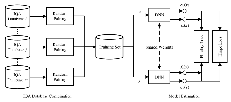
In this section, we first present the proposed training strategy, consisting of IQA database combination and pairwise learning-to-rank model estimation (see Fig. 2). We then describe the details of the UNIQUE model for unified uncertainty-aware BIQA.

III-A IQA Database Combination

Our goal is to combine $m$ IQA databases for training while avoiding additional subjective experiments for perceptual scale realignment. To achieve this, we first randomly sample $n_{j}$ pairs of images $\{(x^{j}_{i},y^{j}_{i})\}_{i=1}^{n_{j}}$ from the $j$-th database. For each image pair $(x,y)$, we infer relative ranking information from the corresponding MOSs and variances. Specifically, under the Thurstone’s model [37], we assume that the true perceptual quality $q(x)$ of image $x$ follows a Gaussian distribution with mean $\mu(x)$ and variance $\sigma^{2}(x)$ collected via subjective testing. Assuming the variability of quality across images is uncorrelated, the quality difference, $q(x)-q(y)$, is also Gaussian with mean $\mu(x)-\mu(y)$ and variance $\sigma^{2}(x)+\sigma^{2}(y)$. The probability that $x$ has higher perceptual quality than $y$ can be calculated from the Gaussian cumulative distribution function $\Phi(\cdot)$:

$$p(x,y)=\Pr({q(x)\geq q(y)})=\Phi\left(\frac{\mu(x)-\mu(y)}{\sqrt{\sigma^{2}(x)+\sigma^{2}(y)}}\right).$$ (1)

Combining pairs of images from $m$ databases, we are able to build a training set $\mathcal{D}=\{\{(x^{j}_{i},y^{j}_{i}),p^{j}_{i}\}_{i=1}^{n_{j}}\}_{j=1}^{m}$. Our database combination approach allows future IQA databases to be added with essentially no cost.

III-B Model Estimation

Given $\mathcal{D}$ as the training set, we aim to learn two differentiable functions $f_{w}(\cdot)$ and $\sigma_{w}(\cdot)$, parameterized by a vector $w$, which accept an image of arbitrary input size, and compute the quality score and the uncertainty, respectively. Similar in Section III-A, we assume the true perceptual quality $q(x)$ obeys a Gaussian distribution with mean and variance now estimated by $f_{w}(x)$ and $\sigma_{w}^{2}(x)$, respectively. The probability of preferring $x$ over $y$ perceptually is

$$p_{w}(x,y)=\Phi\left(\frac{f_{w}(x)-f_{w}(y)}{\sqrt{\sigma_{w}^{2}(x)+\sigma_{w}^{2}(y)}}\right).$$ (2)

It remains to specify a similarity measure between the probability distributions $p(x,y)$ and $p_{w}(x,y)$ as the objective for model estimation. In machine learning, cross-entropy may be the de facto measure for this purpose, but has several drawbacks [12]. First, the minimum of the cross-entropy loss is not exactly zero, except for the ground truth $p(x,y)=0$ and $p(x,y)=1$. This may hinder the learning of image pairs with $p(x,y)$ close to $0.5$. Second, the cross-entropy loss is unbounded from above, which may over-penalize some hard training examples, therefore biasing the learned models. To resolve these issues, we choose the fidelity loss [12], originated from quantum physics [38], as the similarity measure:

$$\ell_{F}(x,y,p;w)=1 -\sqrt{p(x,y)p_{w}(x,y)}$$

$$-\sqrt{(1-p(x,y))(1-p_{w}(x,y))}.$$ (3)

Joint estimation of image quality and uncertainty will introduce scaling ambiguity. More precisely, if we make the scaling $f_{w}(\cdot)\rightarrow\alpha f_{w}(\cdot)$ and $\sigma_{w}(\cdot)\rightarrow\alpha\sigma_{w}(\cdot)$, the probability $p_{w}(x,y)$ given by Eq. (2) is unchanged. Our preliminary results [39] showed that the learned $\sigma_{w}(x)$ by optimizing Eq. (III-B) solely neither resembles any aspects of human behavior in BIQA, nor reveals new statistical properties of natural images. To resolve the scaling ambiguity and provide with $\sigma_{w}(x)$ direct supervision, we enforce a regularizer of $\sigma_{w}(x)$ by taking advantage of the ground truth $\sigma(x)$. Note that the ground truth standard deviations (stds) across IQA databases are not comparable, which prevents the use of their absolute values. Similarly, for each pair $(x,y)$, we infer a binary label $t$ for uncertainty learning, where $t=1$ if $\sigma(x)\geq\sigma(y)$ and $t=-1$ otherwise. We define the regularizer using the hinge loss:

$$\ell_{H}(x,y,t;w)=\max\left(0,\xi-t(\sigma_{w}(x)-\sigma_{w}(y))\right),$$ (4)

where the margin $\xi$ specifies the scale for BIQA models to work with. The augmented training set becomes $\mathcal{D}=\{\{(x^{j}_{i},y^{j}_{i}),p^{j}_{i},t^{j}_{i}\}_{i=1}^{n_{j}}\}_{j=1}^{m}$. During training, we sample a mini-batch $\mathcal{B}$ from $\mathcal{D}$ in each iteration, and use stochastic gradient descent to update the parameter vector $w$ by minimizing the following empirical loss:

$$\ell(\mathcal{B};w)=\frac{1}{|\mathcal{B}|}\sum_{\{(x,y),p,t\}\in\mathcal{B}}\ell_{F}(x,y,p;w)+\lambda\ell_{H}(x,y,t;w),$$ (5)

where $|\mathcal{B}|$ denotes the cardinality of $\mathcal{B}$ and $\lambda$ trades off the two terms.

(a) LIVE

(b) CSIQ

(c) KADID-10K

(d) BID

(e) LIVE Challenge

(f) KonIQ-10K

Figure 3: Scatter plots of means against stds of human quality opinions of images from six IQA databases, including (a) LIVE [4], (b) CSIQ [5], (c) KADID-10K [6], (d) BID [7], (e) LIVE Challenge [8], and (f) KonIQ-10K [9]. There is a clear trend that humans are more consistent (i.e., confident) in making predictions of low-quality and high-quality images than mid-quality images, giving rise to arch-like shapes.

III-C Specification of UNIQUE

We use ResNet-34 [40] as the backbone of UNIQUE due to its good balance between model complexity and capability. Similar to Siamese neural networks [41], the pairwise learning-to-rank framework composed of two streams is shown in Fig. 2. Each stream is implemented by a DNN, consisting of a stage of convolution, batch normalization [42], ReLU nonlinearity, and max-pooling, followed by four residual blocks (see Table III). To generate a fixed-length image representation and summarize higher-order spatial statistics, we replace the first-order average pooling with a second-order bilinear pooling, which has been empirically proven useful in object recognition [43] and BIQA [3]. We flatten the spatial dimensions of the feature representation after the last convolution to obtain $z\in\mathbb{R}^{s\times c}$, where $s$ and $c$ denote the spatial and channel dimensions, respectively. The bilinear pooling can be defined as

$$\bar{z}=z^{T}z.$$ (6)

We further flatten $\bar{z}\in\mathbb{R}^{c\times c}$, and append a fully connected layer with two outputs to represent $f_{w}(x)$ and $\sigma_{w}(x)$, respectively. The network parameters of the two streams are shared during the entire optimization process.

TABLE III: The network architecture of UNIQUE based on ResNet-34 [40]. The nonlinearity and normalization are omitted for brevity

Layer Name	Network Parameter
Convolution	7$\times$7, 64, stride 2
Max Pooling	3$\times$3, stride 2
Residual Block 1	$\left[\begin{array}[]{c}\text{3$\times$3, 64, stride 1}\\[-1.00006pt] \text{3$\times$3, 64, stride 1}\end{array}\right]$$\times$3
Residual Block 2	$\left[\begin{array}[]{c}\text{3$\times$3, 128, stride 2}\\[-1.00006pt] \text{3$\times$3, 128, stride 1}\end{array}\right]$$\times$1
	$\left[\begin{array}[]{c}\text{3$\times$3, 128, stride 1}\\[-1.00006pt] \text{3$\times$3, 128, stride 1}\end{array}\right]$$\times$3
Residual Block 3	$\left[\begin{array}[]{c}\text{3$\times$3, 256, stride 2}\\[-1.00006pt] \text{3$\times$3, 256, stride 1}\end{array}\right]$$\times$1
	$\left[\begin{array}[]{c}\text{3$\times$3, 256, stride 1}\\[-1.00006pt] \text{3$\times$3, 256, stride 1}\end{array}\right]$$\times$5
Residual Block 4	$\left[\begin{array}[]{c}\text{3$\times$3, 512, stride 2}\\[-1.00006pt] \text{3$\times$3, 512, stride 1}\end{array}\right]$$\times$1
	$\left[\begin{array}[]{c}\text{3$\times$3, 512, stride 1}\\[-1.00006pt] \text{3$\times$3, 512, stride 1}\end{array}\right]$$\times$2
Bilinear Pooling	0
Fully Connected Layer	262,144$\times$2

TABLE IV: Median SRCC and PLCC results across ten sessions along with the average absolute deviation in the bracket. CLIVE stands for the LIVE Challenge Database. The databases used for training models are included in the bracket

Database	LIVE [4]	CSIQ [5]	KADID-10K [6]	BID [7]	CLIVE [8]	KonIQ-10K [9]
Criterion	SRCC
MS-SSIM [2]	0.951 ( $\pm$ 0.007)	0.910 ($\pm$ 0.015)	0.821 ( $\pm$ 0.011)	–	–	–
NLPD [44]	0.942 ($\pm$ 0.010)	0.937 ($\pm$ 0.010)	0.822 ($\pm$ 0.013)	–	–	–
DISTS [45]	0.955 ($\pm$ 0.006)	0.944 ($\pm$ 0.015)	0.892 ($\pm$ 0.007)	–	–	–
NIQE [10]	0.906 ($\pm$ 0.013)	0.632 ($\pm$ 0.036)	0.374 ($\pm$ 0.024)	0.468 ($\pm$ 0.081)	0.464 ($\pm$ 0.055)	0.521 ($\pm$ 0.019)
ILNIQE [27]	0.907 ($\pm$ 0.013)	0.832 ($\pm$ 0.030)	0.531 ($\pm$ 0.025)	0.516 ($\pm$ 0.092)	0.469 ($\pm$ 0.047)	0.507 ($\pm$ 0.018)
dipIQ [15]	0.940 ($\pm$ 0.010)	0.511 ($\pm$ 0.036)	0.304 ($\pm$ 0.010)	0.009 ($\pm$ 0.077)	0.187 ($\pm$ 0.047)	0.228 ($\pm$ 0.016)
Ma19 [16]	0.935 ($\pm$ 0.060)	0.917 ($\pm$ 0.043)	0.466 ($\pm$ 0.062)	0.316 ($\pm$ 0.091)	0.348 ($\pm$ 0.048)	0.365 ($\pm$ 0.042)
MEON (LIVE) [32]	–	0.726 ($\pm$ 0.036)	0.234 ($\pm$ 0.035)	0.100 ($\pm$ 0.090)	0.378 ($\pm$ 0.030)	0.145 ($\pm$ 0.015)
deepIQA (LIVE) [31]	–	0.645 ($\pm$ 0.029)	0.270 ($\pm$ 0.041)	-0.043 ($\pm$ 0.105)	0.076 ($\pm$ 0.059)	-0.064 ($\pm$ 0.027)
deepIQA (TID2013)	0.834 ($\pm$ 0.025)	0.679 ($\pm$ 0.043)	0.559 ($\pm$ 0.062)	0.236 ($\pm$ 0.087)	0.048 ($\pm$ 0.048)	0.182 ($\pm$ 0.042)
RankIQA (LIVE) [14]	–	0.711 ($\pm$ 0.011)	0.436 ($\pm$ 0.025)	0.324 ($\pm$ 0.062)	0.451 ($\pm$ 0.047)	0.617 ($\pm$ 0.016)
RankIQA (TID2013)	0.599 ($\pm$ 0.026)	0.667 ($\pm$ 0.079)	0.477 ($\pm$ 0.028)	0.217 ($\pm$ 0.088)	0.289 ($\pm$ 0.051)	0.460 ($\pm$ 0.017)
PQR (BID) [28]	0.663 ($\pm$ 0.069)	0.522 ($\pm$ 0.058)	0.321 ($\pm$ 0.038)	–	0.691 ($\pm$ 0.026)	0.614 ($\pm$ 0.014)
PQR (KADID-10K)	0.916 ($\pm$ 0.016)	0.803 ($\pm$ 0.086)	–	0.358 ($\pm$ 0.081)	0.439 ($\pm$ 0.063)	0.485 ($\pm$ 0.016)
PQR (KonIQ-10K)	0.741 ($\pm$ 0.058)	0.710 ($\pm$ 0.045)	0.583 ($\pm$ 0.025)	0.729 ($\pm$ 0.045)	0.766 ($\pm$ 0.026)	–
PaQ-2-PiQ (LIVE Patch) [46]	0.472 ($\pm$ 0.048)	0.555 ($\pm$ 0.055)	0.379 ($\pm$ 0.026)	0.682 ($\pm$ 0.038)	0.719 ($\pm$ 0.027)	0.722 ($\pm$ 0.009)
DB-CNN (CSIQ) [3]	0.855 ($\pm$ 0.034)	–	0.501 ($\pm$ 0.025)	0.329 ($\pm$ 0.092)	0.451 ($\pm$ 0.056)	0.499 ($\pm$ 0.016)
DB-CNN (LIVE Challenge)	0.723 ($\pm$ 0.044)	0.691 ($\pm$ 0.056)	0.488 ($\pm$ 0.036)	0.809 ($\pm$ 0.023)	–	0.770 ($\pm$ 0.010)
KonCept512 (KonIQ-10K)	0.776 ($\pm$ 0.024)	0.639 ($\pm$ 0.050)	0.491 ($\pm$ 0.033)	0.800 ($\pm$ 0.041)	0.781($\pm$ 0.029)	0.917 ($\pm$ 0.004)
UNIQUE (All databases)	0.969 ($\pm$ 0.008)	0.902 ($\pm$ 0.045)	0.878 ($\pm$ 0.016)	0.858 ($\pm$ 0.032)	0.854 ($\pm$ 0.019)	0.896 ($\pm$ 0.006)
Criterion	PLCC
MS-SSIM [2]	0.941 ($\pm$ 0.006)	0.897 ($\pm$ 0.014)	0.819 ($\pm$ 0.011)	–	–	–
NLPD [44]	0.937 ($\pm$ 0.008)	0.930 ($\pm$ 0.015)	0.821 ($\pm$ 0.014)	–	–	–
DISTS [45]	0.955 ($\pm$ 0.006)	0.946 ($\pm$ 0.015)	0.892 ($\pm$ 0.007)	–	–	–
NIQE [10]	0.908 ($\pm$ 0.013)	0.726 ($\pm$ 0.034)	0.428 ($\pm$ 0.021)	0.461 ($\pm$ 0.073)	0.515 ($\pm$ 0.050)	0.529 ($\pm$ 0.014)
ILNIQE [27]	0.912 ($\pm$ 0.012)	0.873 ($\pm$ 0.026)	0.573 ($\pm$ 0.027)	0.533 ($\pm$ 0.094)	0.536 ($\pm$ 0.030)	0.534 ($\pm$ 0.018)
dipIQ [15]	0.933 ($\pm$ 0.011)	0.778 ($\pm$ 0.020)	0.402 ($\pm$ 0.011)	0.346 ($\pm$ 0.069)	0.290 ($\pm$ 0.042)	0.437 ($\pm$ 0.009)
Ma19 [16]	0.934 ($\pm$ 0.063)	0.926 ($\pm$ 0.024)	0.500 ($\pm$ 0.061)	0.348 ($\pm$ 0.057)	0.400 ($\pm$ 0.047)	0.416 ($\pm$ 0.042)
MEON (LIVE) [32]	–	0.787 ($\pm$ 0.020)	0.410 ($\pm$ 0.007)	0.217 ($\pm$ 0.057)	0.477 ($\pm$ 0.028)	0.242 ($\pm$ 0.014)
deepIQA (LIVE) [31]	–	0.730 ($\pm$ 0.029)	0.309 ($\pm$ 0.059)	0.127 ($\pm$ 0.083)	0.162 ($\pm$ 0.071)	0.088 ($\pm$ 0.027)
deepIQA (TID2013)	0.853 ($\pm$ 0.013)	0.771 ($\pm$ 0.024)	0.573 ($\pm$ 0.061)	0.282 ($\pm$ 0.067)	0.150 ($\pm$ 0.038)	0.272 ($\pm$ 0.042)
RankIQA (LIVE) [14]	–	0.790 ($\pm$ 0.008)	0.488 ($\pm$ 0.017)	0.350 ($\pm$ 0.052)	0.503 ($\pm$ 0.043)	0.631 ($\pm$ 0.014)
RankIQA (TID2013)	0.633 ($\pm$ 0.030)	0.778 ($\pm$ 0.093)	0.504 ($\pm$ 0.031)	0.306 ($\pm$ 0.071)	0.313 ($\pm$ 0.051)	0.471 ($\pm$ 0.015)
PQR (BID) [28]	0.673 ($\pm$ 0.056)	0.612 ($\pm$ 0.032)	0.403 ($\pm$ 0.030)	–	0.740 ($\pm$ 0.014)	0.650 ($\pm$ 0.014)
PQR (KADID-10K)	0.927 ($\pm$ 0.013)	0.870 ($\pm$ 0.051)	–	0.405 ($\pm$ 0.063)	0.501 ($\pm$ 0.051)	0.484 ($\pm$ 0.018)
PQR (KonIQ-10K)	0.760 ($\pm$ 0.060)	0.737 ($\pm$ 0.042)	0.604 ($\pm$ 0.025)	0.739 ($\pm$ 0.039)	0.826 ($\pm$ 0.021)	–
PaQ-2-PiQ (LIVE Patch) [46]	0.559 ($\pm$ 0.037)	0.658 ($\pm$ 0.034)	0.429 ($\pm$ 0.026)	0.713 ($\pm$ 0.030)	0.778 ($\pm$ 0.014)	0.735 ($\pm$ 0.010)
DB-CNN (CSIQ) [3]	0.854 ($\pm$ 0.033)	–	0.569 ($\pm$ 0.023)	0.383 ($\pm$ 0.088)	0.472 ($\pm$ 0.043)	0.515 ($\pm$ 0.015)
DB-CNN (LIVE Challenge)	0.754 ($\pm$ 0.049)	0.685 ($\pm$ 0.050)	0.529 ($\pm$ 0.031)	0.832 ($\pm$ 0.024)	–	0.825 ($\pm$ 0.007)
KonCept512 (KonIQ-10K)	0.772 ($\pm$ 0.019)	0.663 ($\pm$ 0.029)	0.508 ($\pm$ 0.021)	0.818 ($\pm$ 0.031)	0.844($\pm$ 0.023)	0.931 ($\pm$ 0.003)
UNIQUE (All databases)	0.968 ($\pm$ 0.004)	0.927 ($\pm$ 0.032)	0.876 ($\pm$ 0.016)	0.873 ($\pm$ 0.025)	0.890 ($\pm$ 0.011)	0.901 ($\pm$ 0.006)

IV Experiments

In this section, we first present the experimental setups, including the IQA databases, the evaluation protocols, and the training details of UNIQUE. We then compare UNIQUE with several state-of-the-art BIQA models on existing IQA databases as well as the gMAD competition [13]. Moreover, we verify the promise of the proposed training strategy by comparing it with alternative training schemes, testing it in a cross-database setting, and using it to improve existing BIQA models.

IV-A Experimental Setups

We chose six IQA databases (summarized in Table I), among which LIVE [4], CSIQ [5], and KADID-10K [6] contain synthetic distortions, while LIVE Challenge [8], BID [7], and KonIQ-10K [9] include realistic distortions. All selected databases provide the stds of subjective quality scores (see Fig. 3). We excluded TID2013 [47] in our experiments because the MOS is computed by the number of winning times in a maximum of nine paired comparisons without suitable psychometric scaling [48], and does not satisfy the Gaussian assumption. We refer the interested readers to our preliminary work [39] for the results on TID2013 [47].

We randomly sampled $80\%$ images from each database to construct the training set and leave the remaining $20\%$ for testing. Regarding synthetic databases LIVE, CSIQ, and KADID-10K, we split the training and test sets according to the reference images in order to ensure content independence. We adopted two performance criteria: Spearman rank-order correlation coefficient (SRCC) and Pearson linear correlation coefficient (PLCC), which measure prediction monotonicity and precision [49], respectively. To reduce the bias caused by the randomness in training and test set splitting, we repeated this procedure ten times, and reported median SRCC and PLCC results.

We trained UNIQUE on $270,000$ image pairs by minimizing the objective in Eq. (5) using Adam [50]. The margin of the hinge loss $\xi$ and the trade-off parameter $\lambda$ were set to $0.025$ and $1$, respectively. Empirically, we found that the performance is insensitive to the two hyperparameters. We used a softplus function to constrain the predicted std $\sigma_{w}(x)$ to be positive. The parameters of UNIQUE based on ResNet-34 [40] were initialized with the weights pre-trained on ImageNet [51]. The parameters of the last fully connected layer were initialized by He’s method [52]. We set the initial learning rate to $10^{-4}$ with a decay factor of $10$ for every three epochs, and we trained UNIQUE twelve epochs. A warm-up training strategy was adopted: only the last fully connected layer was trained in the first three epochs with a mini-batch of $128$; for the remaining epochs, we fine-tuned the entire method with a mini-batch of $32$. During training, we re-scaled and cropped the images to $384\times 384\times 3$, keeping their aspect ratios. In all experiments, we tested on images of original size. We implemented UNIQUE using PyTorch, and made the code publicly available at https://github.com/zwx8981/UNIQUE.

IV-B Main Results

Figure 4: gMAD competition results between PQR [28] and UNIQUE. The MOS of each image is shown in the bracket. (a) Fixed UNIQUE at the low-quality level. (b) Fixed UNIQUE at the high-quality level. (c) Fixed PQR at the low-quality level. (d) Fixed PQR at the high-quality level.

Figure 5: gMAD competition results between DB-CNN [3] and UNIQUE. The MOS of each image is shown in the bracket. (a) Fixed UNIQUE at the low-quality level. (b) Fixed UNIQUE at the high-quality level. (c) Fixed DB-CNN at the low-quality level. (d) Fixed DB-CNN at the high-quality level.

(a) LIVE

(b) CSIQ

(c) KADID-10K

(d) BID

(e) LIVE Challenge

(f) KonIQ-10K

Figure 6: Scatter plots of means against stds of images from six IQA databases predicted by UNIQUE with the hinge loss. $f_{w}(x)$ and $\sigma_{w}(x)$ indicate the predicted mean and std of image $x$, respectively.

(a) LIVE

(b) CSIQ

(c) KADID-10K

(d) BID

(e) LIVE Challenge

(f) KonIQ-10K

Figure 7: Scatter plots of means against stds of images from six IQA databases predicted by UNIQUE without the hinge loss.

IV-B1 Correlation Results

We compared the performance of UNIQUE against three full-reference IQA measures - MS-SSIM [2], NLPD [44] and DISTS [45], and ten BIQA models, including four knowledge-driven methods that do not require MOSs for training - NIQE [10], IL-NIQE [27], dipIQ [15] and Ma19 [16], and six data-driven DNN-based methods - MEON [32], deepIQA [31], RankIQA [14], PQR [28], PaQ-2-PiQ [46] and DB-CNN [3]. For the competing models, we either used the publicly available implementations or re-trained them on the specific databases using the training codes provided by the corresponding authors [28, 3]. The median SRCC and PLCC results along with the average absolute deviations across ten sessions are listed in Table IV. Note that some methods have been trained on all images from one of the six databases. We thus excluded the corresponding results. NIQE and its improved version ILNIQE do not perform well on realistic distortions and challenging synthetic distortions in KADID-10K [6], despite the original goal of handling arbitrary distortions. dipIQ [15] and Ma19 [16] may only be able to deal with distortions included in the training set. This highlights the difficulty of distortion-aware BIQA methods to handle unseen distortions.

(a) LIVE Challenge, $f_{w}(x)$ = 2.641

(b) KADID-10K, $f_{w}(x)$ = 2.626

(c) KonIQ-10K, $f_{w}(x)$ = 2.520

(d) BID, $f_{w}(x)$ = 1.548

(e) KonIQ-10K, $f_{w}(x)$ = 0.772

(f) CSIQ, $f_{w}(x)$ = 0.417

(g) LIVE, $f_{w}(x)$ = 0.264

(h) BID, $f_{w}(x)$ = 0.107

(i) LIVE Challenge, $f_{w}(x)$ = -2.055

(j) KADID-10K, $f_{w}(x)$ = -2.388

(k) LIVE, $f_{w}(x)$ = -2.785

(l) CSIQ, $f_{w}(x)$ = -2.787

Figure 8: Visual examples from different databases aligned in the learned perceptual scale. (a)-(d) Images with good predicted quality. (e)-(h) Images with fair predicted quality. (i)-(l) Images with poor predicted quality. In each row, images are arranged from left to right in descending order of predicted quality.

We observe similar phenomena for deep learning-based methods when facing the cross-distortion-scenario challenge. Despite large-scale pre-training, MEON fine-tuned on LIVE [4] does not generalize to other databases with different distortion types and scenarios. Being exposed to more synthetic distortion types in TID2013 [47], deepIQA and RankIQA achieve better performance on KADID-10K [6] than MEON. Equipped with a second-order pooling, DB-CNN trained on LIVE Challenge [8] is reasonably good at cross-distortion-scenario generalization. Not surprisingly, PQR, trained on KonIQ-10K with greater content and distortion diversity, generalizes much better to the rest databases than the one trained on BID. The most recent DNN-based method - PaQ-2-PiQ aims for local quality prediction, but only delivers reasonable performance on databases captured in the wild. Relying on more sophisticated InceptionResNetV2 [53], KonCept512 [9] presents promising results on three databases with realistic distortions. Enabled by the proposed training strategy, UNIQUE learns from multiple databases simultaneously, and performs favorably against all competing models on all six databases. It also shows competitive performance when comparing to state-of-the-art full-reference IQA models on synthetic databases.

TABLE V: Median results of UNIQUE trained with and without the hinge loss across ten sessions. The results in the last column are computed by the weighted average across all databases with the weight proportion to the number of images in each database

SRCC	LIVE	CSIQ	KADID-10K	BID	LIVE Challenge	KonIQ-10K	Weighted
UNIQUE trained without the hinge loss	0.969	0.887	0.879	0.872	0.856	0.898	0.889
UNIQUE trained with the hinge loss	0.969	0.902	0.878	0.858	0.854	0.896	0.888
PLCC	LIVE	CSIQ	KADID-10K	BID	LIVE Challenge	KonIQ-10K	Weighted
UNIQUE trained without the hinge loss	0.971	0.893	0.870	0.882	0.897	0.901	0.889
UNIQUE trained with the hinge loss	0.968	0.927	0.876	0.873	0.890	0.901	0.892
Fidelity Loss	LIVE	CSIQ	KADID-10K	BID	LIVE Challenge	KonIQ-10K	Weighted
UNIQUE trained without the hinge loss	0.131	0.086	0.048	0.058	0.015	0.026	0.041
UNIQUE trained with the hinge loss	0.073	0.042	0.020	0.027	0.014	0.010	0.018

TABLE VI: SRCC results on the four IQA databases under the cross-database setup. The subscripts “s” and “r” stand for models trained on KADID-10K [6] and KonIQ-10K [9], respectively. UNIQUE is trained on KADID-10K and KonIQ-10K simultaneously

Database	LIVE	CSIQ	BID	LIVE Challenge
NIQE	0.906	0.627	0.459	0.449
ILNIQE	0.898	0.815	0.496	0.439
dipIQ	0.938	0.527	0.019	0.177
Ma19	0.919	0.915	0.295	0.330
PQRs	0.902	0.765	0.304	0.408
PQRr	0.729	0.707	0.751	0.763
DB-CNNs	0.916	0.751	0.602	0.531
DB-CNNr	0.820	0.724	0.785	0.723
UNIQUE	0.917	0.830	0.783	0.786

IV-B2 gMAD Competition Results

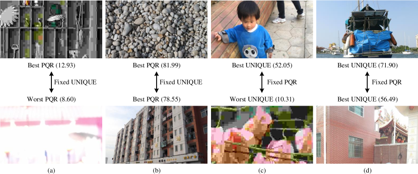
gMAD competition [13] is a complementary methodology for IQA model comparison on large-scale databases without human annotations. Focusing on falsifying perceptual models in the most efficient way, gMAD seeks pairs of images of similar quality predicted by one model, while being substantially different according to another model. To build the playground for gMAD, we combined all synthetically distorted images in the Waterloo Exploration Database [54] with a corpus of realistically distorted images from SPAQ [55]. To quantify the competition results, we also conducted a subjective experiment following ITU-R BT.500 [56], and collected the MOS of each gMAD image. We gathered human data from $16$ subjects using single stimulus continuous quality rating with the range of $[0,100]$. We first let UNIQUE compete against PQR [28] trained on the entire KonIQ-10K [9] in Fig. 4. The pair of images in (a) exhibit similar poor quality, which is in close agreement with UNIQUE. However, PQR favors the top JPEG compressed image, exposing its weaknesses at capturing synthetic distortions. When the roles of the two models are switched, UNIQUE consistently spots the failures of PQR (see (c) and (d)), suggesting that UNIQUE is better able to assess image quality in the laboratory and wild.

TABLE VII: Median SRCC results across ten sessions under different training strategies. MSE stands for the mean squared error

SRCC	LIVE	CSIQ	KADID-10K	BID	LIVE Challenge	KonIQ-10K	Weighted
Baseline (LIVE)	0.951	0.721	0.475	0.632	0.502	0.688	0.596
Baseline (CSIQ)	0.921	0.863	0.483	0.510	0.457	0.638	0.577
Baseline (KADID-10K)	0.877	0.749	0.780	0.498	0.515	0.607	0.693
Baseline (BID)	0.589	0.558	0.298	0.843	0.731	0.722	0.533
Baseline (LIVE Challenge)	0.535	0.504	0.312	0.849	0.842	0.773	0.563
Baseline (KonIQ-10K)	0.832	0.640	0.540	0.765	0.726	0.887	0.716
Linear re-scaling + MSE (All databases)	0.935	0.821	0.870	0.809	0.799	0.868	0.865
Binary labeling + cross entropy (All databases)	0.963	0.863	0.864	0.854	0.860	0.898	0.881
Continuous labeling + cross entropy (All databases)	0.930	0.852	0.713	0.677	0.735	0.788	0.757
UNIQUE (All databases)	0.969	0.902	0.878	0.858	0.854	0.896	0.888

TABLE VIII: Results of one-sided $t$-Test between our training method and binary labeling. A value of $1$ indicates that our method is statistically superior to binary labeling; a value of $-1$ indicates the opposite; a value of $0$ indicates that the two methods are statistically indistinguishable

	LIVE	CSIQ	KADID-10K	BID	LIVE Challenge	KonIQ-10K
Ours versus binary labelling	1	1	1	1	0	0

TABLE IX: Improved SRCC results of DB-CNN across ten sessions enabled by the proposed training strategy

SRCC	LIVE [4]	CSIQ [5]	KADID-10K [6]	BID [7]	LIVE Challenge [8]	KonIQ-10K [9]
DB-CNN (All databases)	0.956	0.912	0.891	0.827	0.836	0.860
Improvements over DB-CNN (CSIQ)	11.81%	–	77.84%	151.37%	85.37%	72.34%
Improvements over DB-CNN (LIVE Challenge)	32.22%	31.98%	82.58%	2.22%	–	11.69%

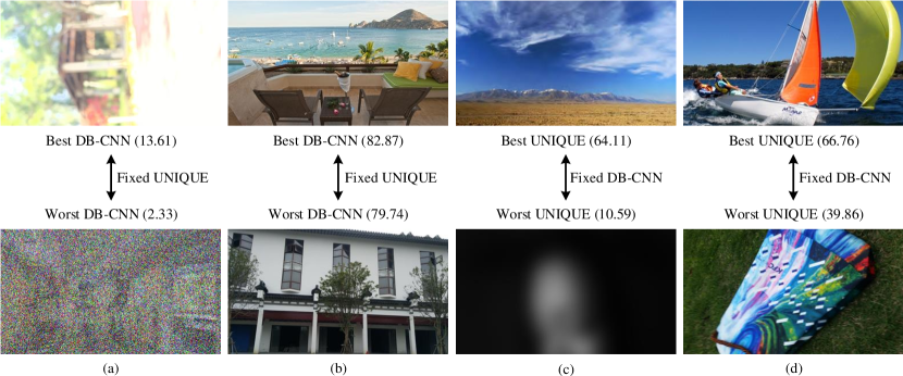
We then let UNIQUE compete with DB-CNN [3], which has demonstrated competitive gMAD performance against other DNN-based BIQA models [32, 31] on the Waterloo Exploration Database. In Fig. 5 (a) and (b), we observe that UNIQUE successfully survives from the attacks by DB-CNN, with images of similar quality according to human perception. DB-CNN [3] fails to penalize the top image in (a), which is severely degraded by a combination of out-of-focus blur and over-exposure. When UNIQUE serves as the attacker, it is able to falsify DB-CNN by finding the counterexamples in (c) and (d). This further validates that UNIQUE well aligns images across distortion scenarios in a learned perceptual scale.

IV-B3 Uncertainty Estimation Results

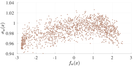
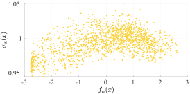
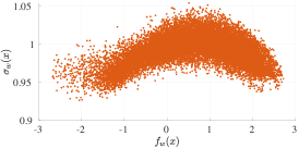
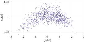
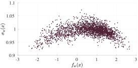
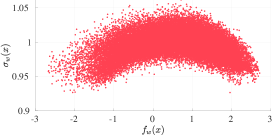
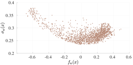
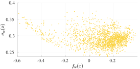
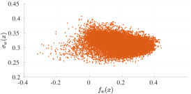
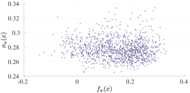
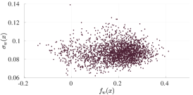
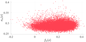
UNIQUE can not only compute image quality scores, but also enable uncertainty quantification of such estimates. We tested the learned uncertainty function $\sigma_{w}(x)$ both quantitatively and qualitatively. To do so, we constructed a baseline version of UNIQUE, which was supervised by the fidelity loss only. That is, no direct supervision of $\sigma_{w}(x)$ is provided, and training may suffer from the scaling ambiguity. In addition to SRCC and PLCC, we also adopted the fidelity loss as a more suitable quantitative measure as it takes into account the ground truth uncertainty when evaluation. Table V shows the median results across ten sessions. Adding the hinge loss as a regularizer, UNIQUE presents a slightly inferior performance in terms of the weighted SRCC ($\approx 0.1\%$), but is significantly better in terms of the fidelity loss ($>56\%$). This suggests that although the hinge loss may pose some constraints on quality estimation, it is helpful in regularizing the uncertainty learning of UNIQUE. We also draw the scatter plots of the learned uncertainty $\sigma_{w}(x)$ as a function of $f_{w}(x)$ in Fig. 6. With the hinge regularizer, the learned uncertainty on all databases exhibits human-like behavior, in that UNIQUE tends to assess images in the two ends of the quality range with higher confidence (i.e., lower uncertainty). In contrast, without the hinge regularizer, the learned uncertainty is less interpretable.

IV-B4 Qualitative Results

We conducted a qualitative analysis of UNIQUE by sampling images across different databases, as shown in Fig. 8. Although the proposed training strategy does not generate pairs of images from two different databases, the optimized UNIQUE is capable of aligning images from different databases in a perceptually meaningful way. In particular, synthetically distorted images with severe levels that may not encounter in the real world receive the lowest quality scores, conforming to our observations that the ranges of $f_{w}(x)$ in LIVE [4], CSIQ [5] and KADID-10K [6] are relatively broader.

IV-C Ablation Studies

IV-C1 Performance in a Cross-Database Setting

We tested UNIQUE in a more challenging cross-database setting. Specifically, we constructed another training set $\mathcal{D}^{\prime}$ using image pairs sampled from the full KADID-10K [6] and KonIQ-10K [9] databases, and re-trained it with the procedure described in IV-A. As comparison, we also re-trained two top-performing DNN-based methods - PQR [28] and DB-CNN [3] on the full KADID-10K [6] and KonIQ-10K [9] databases. The full LIVE [4], CSIQ [5], BID [7], and LIVE Challenge [8] were employed as the test sets. It is clear from Table VI that UNIQUE achieves significantly better performance than the four knowledge-driven models and the two DNN-based models. The training image pairs from the two databases effectively provide mutual regularization, guiding UNIQUE to a better local optimum. This experiment provides strong evidence that UNIQUE enabled by the proposed training strategy generalizes to both synthetic and realistic distortions.

IV-C2 Performance of Different Training Strategies

The key idea of UNIQUE to meet the cross-distortion-scenario challenge is to train it on multiple databases. Here we compared different training strategies against the proposed one. We first treated BIQA as a standard regression problem, and trained six variants of UNIQUE on six databases separately using the mean squared error (MSE) as the loss. Next, we turned to exploit the idea of training BIQA models on multiple databases simultaneously. As discussed in Section I, we linearly re-scaled the MOSs to the same range of $[0,100]$, and re-trained the network using MSE. We also computed binary labels using MOSs: for an image pair $(x,y)$, the ground truth is $r=1$ if $u(x)\geq u(y)$ and $r=0$ otherwise. We re-trained the model using the cross entropy loss. We further trained a variant of UNIQUE by replacing the fidelity loss with the cross-entropy loss. The results are listed in Table VII. We find that regression-based models perform favorably on the training databases, present reasonable generalization to databases of similar distortion scenarios, but show incompetence in cross-distortion-scenario generalization. Training on multiple databases lead to a significant performance boost. It is quite surprising that continuous labeling with the cross entropy loss offers the least improvement, even underperforming linear re-scaling. This may be due to the instability of the cross entropy function when dealing with continuous annotations [12]. By contrast, binary labeling achieves better performance, but is still inferior to the proposed training strategy in terms of the weighted SRCC. We also conducted a $t$-test [57] on the SRCC values of all databases obtained from the ten sessions to examine whether the performance difference between our method and binary labeling is statistically significant. The null hypothesis is that the mean SRCC of our method is statistically indistinguishable from the mean SRCC of binary labeling with a confidence of $95\%$. From Table VIII, we observe that our training method delivers statistically superior performance on LIVE, CSIQ, KADID-10K, and BID, while is statistically on par with binary labeling on the remaining two databases.

IV-C3 Improving Existing BIQA Models

The proposed training strategy is model-agnostic, meaning that it can be used to fine-tune existing differentiable BIQA models for improved performance. Here we implement this idea by applying the proposed training strategy to DB-CNN [3]. The SRCC results are shown in Table IX. We find that DB-CNN fine-tuned by the proposed training strategy achieves significantly better performance than the original versions trained on CSIQ and LIVE challenge, where the improvement can be as high as $151.37\%$. From this experiment, we may conclude that the improvement by the proposed training strategy is orthogonal to the network architecture design.

V Conclusion

We have introduced a unified uncertainty-aware BIQA model - UNIQUE, and a method of training it on multiple IQA databases simultaneously. We also proposed an uncertainty regularizer, which enables direct supervision from the ground truth human uncertainty. UNIQUE is the first of its kind with superior cross-distortion-scenario generalization. We believe this performance improvements arise because of 1) the continuous ranking annotation that provides a more accurate supervisory signal, 2) the fidelity loss that assigns appropriate penalties to image pairs with different probabilities, and 3) the hinge regularizer that offers better statistical modeling of the uncertainty. In the future, we hope that the proposed learning strategy will become a standard solution for existing and next-generation BIQA models to meet the cross-distortion-scenario challenge. We also would like to explore the limits of the proposed learning strategy, towards universal visual quality assessment of digital images and videos in various multimedia applications.

References

- [1] Z. Wang and A. C. Bovik, Modern Image Quality Assessment. Morgan & Claypool, 2006.
- [2] Z. Wang, E. P. Simoncelli, and A. C. Bovik, “Multiscale structural similarity for image quality assessment,” in IEEE Asilomar Conference on Signals, Systems and Computers, 2003, pp. 1398–1402.
- [3] W. Zhang, K. Ma, J. Yan, D. Deng, and Z. Wang, “Blind image quality assessment using a deep bilinear convolutional neural network,” IEEE Transactions on Circuits and Systems for Video Technology, vol. 30, no. 1, pp. 36–47, Jan. 2020.
- [4] H. R. Sheikh, M. F. Sabir, and A. C. Bovik, “A statistical evaluation of recent full reference image quality assessment algorithms,” IEEE Transactions on Image Processing, vol. 15, no. 11, pp. 3440–3451, Nov. 2006.
- [5] E. C. Larson and D. M. Chandler, “Most apparent distortion: Full-reference image quality assessment and the role of strategy,” Journal of Electronic Imaging, vol. 19, no. 1, pp. 1–21, Jan. 2010.
- [6] H. Lin, V. Hosu, and D. Saupe, “KADID-10k: A large-scale artificially distorted IQA database,” in International Conference on Quality of Multimedia Experience, 2019, pp. 1–3.
- [7] A. Ciancio, A. L. N. T. Targino da Costa, E. A. B. da Silva, A. Said, R. Samadani, and P. Obrador, “No-reference blur assessment of digital pictures based on multifeature classifiers,” IEEE Transactions on Image Processing, vol. 20, no. 1, pp. 64–75, Jan. 2011.
- [8] D. Ghadiyaram and A. C. Bovik, “Massive online crowdsourced study of subjective and objective picture quality,” IEEE Transactions on Image Processing, vol. 25, no. 1, pp. 372–387, Jan. 2016.
- [9] V. Hosu, H. Lin, T. Sziranyi, and D. Saupe, “KonIQ-10k: An ecologically valid database for deep learning of blind image quality assessment,” IEEE Transactions on Image Processing, vol. 29, pp. 4041–4056, Jan. 2020.
- [10] A. Mittal, R. Soundararajan, and A. C. Bovik, “Making a ’Completely Blind’ image quality analyzer,” IEEE Signal Processing Letters, vol. 20, no. 3, pp. 209–212, Mar. 2013.
- [11] Q. Wu, H. Li, K. N. Ngan, and K. Ma, “Blind image quality assessment using local consistency aware retriever and uncertainty aware evaluator,” IEEE Transactions on Circuits and Systems for Video Technology, vol. 28, no. 9, pp. 2078–2089, Sep. 2018.
- [12] M.-F. Tsai, T.-Y. Liu, T. Qin, H.-H. Chen, and W.-Y. Ma, “FRank: A ranking method with fidelity loss,” in International ACM SIGIR Conference on Research and Development in Information Retrieval, 2007, pp. 383–390.
- [13] K. Ma, Z. Duanmu, Z. Wang, Q. Wu, W. Liu, H. Yong, H. Li, and L. Zhang, “Group maximum differentiation competition: Model comparison with few samples,” IEEE Transactions on Pattern Analysis and Machine Intelligence, vol. 42, no. 4, pp. 851–864, Apr. 2020.
- [14] X. Liu, J. v. d. Weijer, and A. D. Bagdanov, “RankIQA: Learning from rankings for no-reference image quality assessment,” in IEEE International Conference on Computer Vision, 2017, pp. 1040–1049.
- [15] K. Ma, W. Liu, T. Liu, Z. Wang, and D. Tao, “dipIQ: Blind image quality assessment by learning-to-rank discriminable image pairs,” IEEE Transactions on Image Processing, vol. 26, no. 8, pp. 3951–3964, Aug. 2017.
- [16] K. Ma, X. Liu, Y. Fang, and E. P. Simoncelli, “Blind image quality assessment by learning from multiple annotators,” in IEEE International Conference on Imaging Processing, 2019, pp. 2344–2348.
- [17] F. Gao, D. Tao, X. Gao, and X. Li, “Learning to rank for blind image quality assessment,” IEEE Transactions on Neural Networks and Learning Systems, vol. 26, no. 10, pp. 2275–2290, Oct. 2015.
- [18] G. Zhai and X. Min, “Perceptual image quality assessment: a survey,” Science China Information Sciences, vol. 63, pp. 1–52, Apr. 2020.
- [19] Z. Wang, H. R. Sheikh, and A. C. Bovik, “No-reference perceptual quality assessment of JPEG compressed images,” in IEEE International Conference on Image Processing, vol. 1, 2002, pp. I–I.
- [20] P. Marziliano, F. Dufaux, S. Winkler, and T. Ebrahimi, “Perceptual blur and ringing metrics: application to JPEG2000,” Signal Processing: Image Communication, vol. 19, no. 2, pp. 163–172, Feb. 2004.
- [21] A. K. Moorthy and A. C. Bovik, “Blind image quality assessment: From natural scene statistics to perceptual quality,” IEEE Transactions on Image Processing, vol. 20, no. 12, pp. 3350–3364, Dec. 2011.
- [22] P. Ye, J. Kumar, L. Kang, and D. Doermann, “Unsupervised feature learning framework for no-reference image quality assessment,” in IEEE Conference on Computer Vision and Pattern Recognition, 2012, pp. 1098–1105.
- [23] A. Mittal, A. K. Moorthy, and A. C. Bovik, “No-reference image quality assessment in the spatial domain,” IEEE Transactions on Image Processing, vol. 21, no. 12, pp. 4695–4708, Dec. 2012.
- [24] J. Xu, P. Ye, Q. Li, H. Du, Y. Liu, and D. Doermann, “Blind image quality assessment based on high order statistics aggregation,” IEEE Transactions on Image Processing, vol. 25, no. 9, pp. 4444–4457, Sep. 2016.
- [25] D. Ghadiyaram and A. C. Bovik, “Perceptual quality prediction on authentically distorted images using a bag of features approach,” Journal of Vision, vol. 17, no. 1, pp. 32–32, Jan. 2017.
- [26] E. P. Simoncelli and B. A. Olshausen, “Natural image statistics and neural representation,” Annual Review of Neuroscience, vol. 24, no. 1, pp. 1193–1216, Aug. 2001.
- [27] L. Zhang, L. Zhang, and A. C. Bovik, “A feature-enriched completely blind image quality evaluator,” IEEE Transactions on Image Processing, vol. 24, no. 8, pp. 2579–2591, Aug. 2015.
- [28] H. Zeng, L. Zhang, and A. C. Bovik, “Blind image quality assessment with a probabilistic quality representation,” in IEEE International Conference on Image Processing, 2018, pp. 609–613.
- [29] H. Zhu, L. Li, J. Wu, W. Dong, and G. Shi, “MetaIQA: Deep meta-learning for no-reference image quality assessment,” in IEEE Conference on Computer Vision and Pattern Recognition, 2020, pp. 14 131–14 140.
- [30] L. Kang, P. Ye, Y. Li, and D. Doermann, “Convolutional neural networks for no-reference image quality assessment,” in IEEE Conference on Computer Vision and Pattern Recognition, 2014, pp. 1733–1740.
- [31] S. Bosse, D. Maniry, K. R. Müller, T. Wiegand, and W. Samek, “Deep neural networks for no-reference and full-reference image quality assessment,” IEEE Transactions on Image Processing, vol. 27, no. 1, pp. 206–219, Jan. 2018.
- [32] K. Ma, W. Liu, K. Zhang, Z. Duanmu, Z. Wang, and W. Zuo, “End-to-end blind image quality assessment using deep neural networks,” IEEE Transactions on Image Processing, vol. 27, no. 3, pp. 1202–1213, Mar. 2018.
- [33] Z. Wang and K. Ma, “Active fine-tuning from gMAD examples improves blind image quality assessment,” CoRR, vol. abs/2003.03849, 2020.
- [34] B. Hu, L. Li, H. Liu, W. Lin, and J. Qian, “Pairwise-comparison-based rank learning for benchmarking image restoration algorithms,” IEEE Transactions on Multimedia, vol. 21, no. 8, pp. 2042–2056, Aug. 2019.
- [35] A. Kendall and Y. Gal, “What uncertainties do we need in bayesian deep learning for computer vision,” in Advances in Neural Information Processing Systems, 2017, pp. 5580–5590.
- [36] Y. Huang, X. Tian, R. Jiang, and Y. Chen, “Convolutional neural network with uncertainty estimates for no-reference image quality assessment,” in International Conference on Graphics and Image Processing, 2019, pp. 1–8.
- [37] L. L. Thurstone, “A law of comparative judgment,” Psychological Review, vol. 34, pp. 273–286, Jul. 1927.
- [38] N. Birrell and P. Davies, Quantum Fields in Curved Space. Cambridge University Press, 1984.
- [39] W. Zhang, K. Ma, G. Zhai, and X. Yang, “Learning to blindly assess image quality in the laboratory and wild,” in IEEE International Conference on Image Processing, 2020, pp. 111–115.
- [40] K. He, X. Zhang, S. Ren, and J. Sun, “Deep residual learning for image recognition,” in IEEE Conference on Computer Vision and Pattern Recognition, 2016, pp. 770–778.
- [41] B. Jane, G. Isabelle, L. Yann, S. Eduard, and S. Roopak, “Signature verification using a” siamese” time delay neural network,” in Advances in Neural Information Processing Systems, 1994, pp. 737–744.
- [42] S. Ioffe and C. Szegedy, “Batch normalization: Accelerating deep network training by reducing internal covariate shift,” in International Conference on Machine Learning, 2015, pp. 448–456.
- [43] T.-Y. Lin, A. RoyChowdhury, and S. Maji, “Bilinear CNN models for fine-grained visual recognition,” in IEEE International Conference on Computer Vision, 2015, pp. 1449–1457.
- [44] V. Laparra, A. Berardino, J. Ballé, and E. P. Simoncelli, “Perceptually optimized image rendering,” Journal of the Optical Society of America A: Optics and Image Science, and Vision, vol. 34, pp. 1511–1525, Sep. 2017.
- [45] K. Ding, K. Ma, S. Wang, and E. P. Simoncelli, “Image quality assessment: Unifying structure and texture similarity,” IEEE Transactions on Pattern Analysis and Machine Intelligence, vol. to appear, 2020.
- [46] Z. Ying, H. Niu, P. Gupta, D. Mahajan, D. Ghadiyaram, and A. C. Bovik, “From patches to pictures (PaQ-2-PiQ): Mapping the perceptual space of picture quality.” in IEEE Conference on Computer Vision and Pattern Recognition, 2020, pp. 3572–3582.
- [47] P. Nikolay, J. Lina, I. Oleg, L. Vladimir, E. Karen, A. Jaakko, V. Benoit, C. Kacem, C. Marco, B. Federica, and C.-C. J. Kuo, “Image database TID2013: Peculiarities, results and perspectives,” Signal Processing: Image Communication, vol. 30, pp. 57–77, Jan. 2015.
- [48] M. Aliaksei, P.-O. María, and M. Rafal, “Psychometric scaling of TID2013 dataset,” in IEEE International Conference on Quality of Multimedia Experience, 2018, pp. 1–6.
- [49] Z. Gao, G. Zhai, H. Deng, and X. Yang, “Extended geometric models for stereoscopic 3d with vertical screen disparity,” Displays, vol. 65, p. 101972, Dec. 2020.
- [50] D. P. Kingma and J. Ba, “Adam: A method for stochastic optimization,” CoRR, vol. abs/1412.6980, 2014.
- [51] J. Deng, W. Dong, R. Socher, L.-J. Li, K. Li, and F.-F. Li, “ImageNet: A large-scale hierarchical image database,” in IEEE Conference on Computer Vision and Pattern Recognition, 2009, pp. 248–255.
- [52] K. He, X. Zhang, S. Ren, and J. Sun, “Delving deep into rectifiers: Surpassing human-level performance on ImageNet classification,” in IEEE International Conference on Computer Vision, 2015, pp. 1026–1034.
- [53] S. Christian, V. Vincent, I. Sergey, S. Jon, and W. Zbigniew, “Rethinking the inception architecture for computer vision,” in IEEE Conference on Computer Vision and Pattern Recognition, 2016, pp. 2818–2826.
- [54] K. Ma, Z. Duanmu, Q. Wu, Z. Wang, H. Yong, H. Li, and L. Zhang, “Waterloo Exploration Database: New challenges for image quality assessment models,” IEEE Transactions on Image Processing, vol. 26, no. 2, pp. 1004–1016, Feb. 2017.
- [55] Y. Fang, H. Zhu, Y. Zeng, K. Ma, and Z. Wang, “Perceptual quality assessment of smartphone photography,” in IEEE Conference on Computer Vision and Pattern Recognition, 2020, pp. 3677–3686.
- [56] VQEQ, “Final report from the video quality experts group on the validation of objective models of video quality assessment,” [Online], 2000, Available: http://www.vqeg.org/.
- [57] S. David J, Handbook of Parametric and Nonparametric Statistical Procedures. CRC Press, 2004.