Minimally Modified Gravity fitting Planck data better than $\Lambda$CDM

Abstract

We study the phenomenology of a class of minimally modified gravity theories called $f(\mathcal{H})$ theories, in which the usual general relativistic Hamiltonian constraint is replaced by a free function of it. After reviewing the construction of the theory and a consistent matter coupling, we analyze the dynamics of cosmology at the levels of both background and perturbations, and present a concrete example of the theory with a $3$-parameter family of the function $f$. Finally, we compare this example model to Planck data as well as some later-time probes, showing that such a realization of $f(\mathcal{H})$ theories fits the data significantly better than the standard $\Lambda$CDM model, in particular by modifying gravity at intermediate redshifts, $z\simeq 743$.

I Introduction

The $\Lambda\text{CDM}$ model for cosmology depends on 6 parameters Kosowsky:2002zt ; Durrer:2008eom . Various features of our universe are successfully described by the $\Lambda\text{CDM}$ model. Setting aside the cosmological constant problem and other theoretical issues, it provides us the simplest description of the universe with the cosmic microwave background radiation, the large-scale structure and the accelerated expansion, the last of which we probe for example by supernovae observations. Up to now, this model is still considered the best fitting model to the cosmological data sets.

Despite the success of the $\Lambda\text{CDM}$ model to describe our universe, it faces tensions in explaining a few parameters from various cosmological data sets. This situation motivates us to consider models beyond $\Lambda\text{CDM}$. The most famous and significant tension lies between the estimation of today’s Hubble expansion parameter $H_{0}$ from Planck data Bernal:2016gxb , and its measurement from observations of the local universe, such as those from the Hubble Space Telescope (HST) Riess:2019cxk , H$0$LiCOW Wong:2019kwg , Megamaser Cosmology Project (MCP) Reid:2008nm , Carnegie-Chicago Hubble Program (CCHP) Collaboration Freedman:2019jwv , etc. The significance of this first tension goes up to $5.3\sigma$ Wong:2019kwg . This discrepancy can be understood as a tension between late time data, which do not assume any prior cosmological model, and early universe data, which assume a prior model, i.e. the $\Lambda\text{CDM}$. It comes to light as the early universe and the late time observations (HST) have achieved greater precision in their measurements. At present, there are several approaches to resolve this particular tension, including modified gravity (see  DeFelice:2020sdq ; Ballardini:2020iws ; Braglia:2020iik for example), or adding new types of matter content (as early dark energy Poulin2019 for example).

The number two tension lies between the estimation of the growth of structure $S_{8}$ from Planck data and that from the redshift space distortion data. The disagreement has a statistical significance of up to $3.2\sigma$ Asgari:2019fkq . There are several investigations to address this issue from the perspective of modified gravity theories DeFelice:2016ufg ; DeFelice:2020icf .

Two other results could fit the bill as tensions within the $\Lambda$CDM model. The Planck 2018 result has reported a preference for a higher lensing amplitude Motloch:2018pjy ; Motloch:2019gux . This anomaly has been argued to be related to a new possible tension in the $\Lambda\text{CDM}$ model of cosmology, known as $\Omega_{K}$ tension, which is investigated in Handley:2019tkm ; DiValentino:2019qzk ; DiValentino:2020hov . In fact the Planck collaboration also has reported that the Planck data alone prefers a closed universe Aghanim:2018eyx . In DiValentino:2020hov , it has been found that the curvature parameter of the universe is in tension with the Planck+late time data and BAO data sets. In their investigation they have found better fit to closed universe than $\Lambda\text{CDM}$.

The cosmological tensions arising within $\Lambda\text{CDM}$ can be interpreted as the indication that $\Lambda\text{CDM}$ may be only a first approximation to a more accurate theory of cosmology. In this context it is worth investigating the cosmology of modified theories of gravity to address these various tensions. As mentioned, there have been several attempts which rely on modified theories of gravity. In this work, we focus on a certain class of modified theories of gravity in which there are only two local gravitational degrees of freedom propagating, dubbed minimally modified gravity (MMG) theories in Lin:2017oow and then further developed in Aoki:2018zcv ; Aoki:2018brq ; Mukohyama:2019unx ; DeFelice:2020eju (see DeFelice:2015hla ; DeFelice:2015moy ; Bolis:2018vzs ; DeFelice:2018vza for an earlier example with two local gravitational degrees of freedom in the context of massive gravity and also Afshordi:2006ad ; Iyonaga:2018vnu ; Feng:2019dwu ; Gao:2019twq ; Aoki:2020lig for more examples of MMG theories). These theories break four dimensional diff-invariance keeping the three dimensional diff-invariance so that the standard framework of cosmological studies can be applied. Even though breaking four dimensional diff-invariance leads, in general, to new degrees of freedom in addition to the usual two gravitational modes, MMG theories have Hamiltonians linear in the lapse function so that they come with a Hamiltonian constraint that will reduce the dimension of the physical phase space and leave only two tensorial modes in the theory.

Recently there has been a Hamiltonian construction for a class of MMG theories, dubbed $f(\mathcal{H})$ theories Mukohyama:2019unx , in which the standard Hamiltonian constraint $\mathcal{H}$ of general relativity (GR) is modified to a free function $f(\mathcal{H})$. This leads to changing the kinetic structure of the theory from GR in a background-dependent way and provides an opportunity to address the cosmological tensions.

In this article we study the cosmology in $f(\mathcal{H})$ theories, considering a model that we have named “kink” model as it has a kink in the first derivative of the free function $f^{\prime}\left(\mathcal{H}\right)$. We introduce a consistent coupling to matter which relies on a gauge fixing in the Hamiltonian as it was done in Aoki:2018zcv ; Carballo-Rubio:2018czn , and we study linear perturbations so that we can exhibit the no ghost conditions. We then implement the scalar linear perturbation equations in the Boltzmann code called CLASS Blas:2011rf , with covariantly corrected baryon equations of motion Pookkillath:2019nkn . Subsequently a Monte Carlo sampling, using MontePython Brinckmann:2018cvx ; Audren:2012wb , is done against various cosmological data sets. We consider data of Planck 2018 with planck_highl_TTTEEE, planck_lowl_EE, planck_lowl_TT polarization Aghanim:2019ame ; Akrami:2019izv ; Aghanim:2018eyx ; Akrami:2018odb ; Aghanim:2018oex , of HST observations Riess:2019cxk consisting in the single data point of the Hubble constant $H_{0}=74.03_{-1.42}^{+1.42}$, of the baryon acoustic oscillation (BAO) from 6dF Galaxy Survey Beutler:2011hx and the Sloan Digital Sky Survey Ross:2014qpa ; Alam:2016hwk , and of the joint light curves (JLA) comprised of 740 type Ia supernovae Betoule:2014frx . We refer to all these data sets as Planck2018+HST+BAO+JLA. The chains are then analyzed using the well-suited GetDist package Lewis:2019xzd . We find that there is a remarkable improvement with respect to $\Lambda\text{CDM}$ in the likelihood-parameter $\chi^{2}$ with a difference of $\Delta\chi^{2}=16.6$ for the chosen data sets. Although there is only a minimal improvement for the $H_{0}$ tension, the other tensions that have appeared within $\Lambda$CDM have a chance to be addressed by the $f(\mathcal{H})$ theory.

This paper is organized as follows. In section II, we review $f(\mathcal{H})$ theories from their inception, and discuss the particular matter coupling that has to be adopted to avoid the propagation of unwanted degrees of freedom. In section III, we use the Lagrangian introduced in section II to derive the dynamics of the cosmological background, as well as its perturbations. In section IV, we propose a concrete model where the function $f$ depends on three free parameters and has a kink in its first derivative. As we will show subsequently, such a model has a very good fit to cosmological data. Then, in section V we show that the kink model consistently gives a better fitness parameter than $\Lambda$CDM, considering both early and late time cosmological data sets together. This comparison is the main result of this paper. Finally, we conclude in section VI with a summary of results and a discussion.

II Minimally Modified Gravity and $f(H)$ theories

Minimally modified gravity (MMG) theories are modifications of four-dimensional GR with two local gravitational degrees of freedom. A systematic construction of gravitational theories with only (up to) two degrees of freedom has been initiated in Lin:2017oow ; Aoki:2018zcv ; Aoki:2018brq (see also Carballo-Rubio:2018czn for a different perspective). The idea consists in renouncing the invariance under four dimensional diffeomorphisms but keeping the three dimensional (spatial) diff-invariance. As generically Lorentz-breaking gravity theories have more than two degrees of freedom, one has to find the conditions for the theory to possess enough constraints that would kill the extra degrees of freedom, which would leave us with (at most) two gravitational modes only. This section is devoted to review these conditions following Mukohyama:2019unx .

In the first part, we will quickly recall the basis of the construction of MMG theories as it was done in Mukohyama:2019unx where the Hamiltonian point of view was adopted. Then, we will show how $f(\mathcal{H})$ theories naturally emerge as simple but interesting examples of MMG theories. Finally, we will explain how to couple matter to these theories without introducing new degrees of freedom in the gravitational sector, following the construction developed in Aoki:2018zcv ; Aoki:2018brq .

II.1 Modifying the phase space

The construction of the $f({\cal H})$ class of MMG theories presented in Mukohyama:2019unx relies on the Hamiltonian formulation of GR. The idea consists in modifying the phase space of GR, and not directly the Lagrangian, in such a way that the modified theory remains invariant under spatial diffeomorphisms only but still propagates two tensorial degrees of freedom.

Hence, we start with the Arnowitt-Deser-Misner (ADM) parametrization of the metric,

$$ds^{2}\;=\;-N^{2}dt^{2}+\gamma_{ij}(dx^{i}+N^{i}dt)(dx^{j}+N^{j}dt)\,,$$ (1)

in terms of the lapse function $N$, the shift vector $N^{i}$ and the induced spatial metric $\gamma_{ij}$. Hereafter, we will denote by $D_{i}$ the covariant derivative compatible with $\gamma_{ij}$, we will lower and raise spatial indices by the metric $\gamma_{ij}$ and its inverse $\gamma^{ij}$, and we will use the notation $\gamma$ for the determinant of the spatial metric.

The phase space is parametrized by the usual ten pairs of conjugate variables,

$$\{\gamma_{ij}(x),\pi^{kl}(y)\}=\frac{1}{2}(\delta_{i}^{k}\delta_{j}^{l}+\delta_{i}^{l}\delta_{j}^{k})\,\delta(x-y)\,,$$

$$\{N^{i}(x),\pi_{j}(y)\}=\delta_{j}^{i}\,\delta(x-y)\,,$$ (2)

$$\{N(x),\pi_{N}(y)\}=\delta(x-y)\,,$$

where $\pi^{ij}$, $\pi_{i}$ and $\pi_{N}$ are momenta, and $\delta(x-y)$ is the 3-dimensional $\delta$-distribution.

In GR, $N$ and $N^{i}$ are Lagrange multipliers, thus their conjugate momenta $\pi_{N}$ and $\pi_{i}$ vanish, which produces a set of four primary constraints,

$$\pi_{N}\,\approx\,0\,,\qquad\pi_{i}\,\approx\,0\,.$$ (3)

We are using the notation $\approx$ for the weak equality in the phase space, i.e. the equality up to constraints. Concerning the momenta conjugate to $\gamma_{ij}$, they are easily related to the extrinsic curvature tensor by,

$$\pi^{ij}=\sqrt{\gamma}\left(K^{ij}-K\gamma^{ij}\right)\,,\qquad K_{ij}\equiv\frac{1}{2N}\left(\dot{\gamma}_{ij}-D_{i}N_{j}-D_{j}N_{i}\right)\,,$$ (4)

with $K\equiv K^{i}{}_{i}$ being the trace of the extrinsic curvature. As a consequence, one can immediately compute the Hamiltonian of GR which takes the very well-known form,

$$H\;=\;\int d^{3}x\sqrt{\gamma}\left(N{\cal H}_{0}+N^{i}{\cal H}_{i}\right)\,,$$ (5)

where the Hamiltonian constraint ${\cal H}_{0}$ and the vectorial (momentum) constraints ${\cal H}_{i}$ are given by,

$${\cal H}_{0}\equiv\frac{1}{\gamma}\left(\pi_{ij}\pi^{ij}-\frac{1}{2}\pi^{2}\right)-R\,,\qquad{\cal H}_{i}\equiv-2D^{j}\left(\frac{\pi_{ij}}{\sqrt{\gamma}}\right)\,,$$ (6)

with $R$ being the spatial curvature of the metric $\gamma_{ij}$. The conservation under time evolution of the primary constraints (3) leads to the secondary constraints ${\cal H}_{0}\approx 0$ and ${\cal H}_{i}\approx 0$, which form together with (3) a set of first class constraints. The Hamiltonian analysis closes here: as we started with 10 pairs of variables (2) and we found 8 first class constraints, we end up with the expected 2 tensorial degrees of freedom of GR.

In Mukohyama:2019unx , one proposed a deformation of the phase space of GR requiring that the modified theory remains invariant under spatial diffeomorphisms only yet still propagates two tensorial degrees of freedom. In this approach, one starts with the same (non-physical) phase space parametrized by the usual ten pairs of conjugate variables (2) and one looks for a total Hamiltonian of the form,

$$H_{{\rm def}}\;=\;\int d^{3}x\sqrt{\gamma}\left[{\cal S}(\gamma_{ij},\pi^{ij},R_{ij},N,D_{i})+N^{i}{\cal H}_{i}\right]\,,$$ (7)

where ${\cal S}$ is a three-dimensional scalar constructed from the variables $(\gamma_{ij},\pi^{ij},R_{ij},N)$ and their spatial derivatives. It was implicitly assumed that neither $N$ nor $N^{i}$ are dynamical variables. Requiring that the theory propagates only two degrees of freedom (or less) leads necessarily to the condition that ${\cal S}$ is an affine function of $N$, i.e.

$${\cal S}(\gamma_{ij},\pi^{ij},R_{ij},N,D_{i})\;=\;{\cal V}(\gamma_{ij},\pi^{ij},R_{ij},D_{i})+N\,{\cal H}_{0{\rm def}}(\gamma_{ij},\pi^{ij},R_{ij},D_{i})\,,$$ (8)

which is, of course, compatible with the fact that $N$ is not dynamical. Hence, ${\cal H}_{0{\rm def}}$ can be viewed as a deformation of the usual Hamiltonian constraint of general relativity whereas ${\cal V}$ is a new term. However, the functions ${\cal V}$ and ${\cal H}_{0{\rm def}}$ are not arbitrary and must satisfy extra conditions to ensure that no degrees of freedom other than the two tensor modes propagate Mukohyama:2019unx . Even though these conditions have not been solved in full generality and rigor, it was shown that any theory whose Hamiltonian is given by (7) with

$$\{{\cal H}_{0{\rm def}}(x)\,,\,{\cal H}_{0{\rm def}}(y)\}\,\approx\,0\,,$$ (9)

while ${\cal V}$ is totally free, defines a MMG theory. In other words, (9) is a sufficient condition for the theory defined by the Hamiltonian (7) to propagate (at most) two degrees of freedom.

II.2 Deforming the Hamiltonian constraint: $f(\mathcal{H})$ theories

Finding all the functions ${\cal H}_{0{\rm def}}(\gamma_{ij},\pi^{ij},R_{ij},N,D_{i})$ which satisfy (9) seems a priori to be a highly complicated problem. The reason is that, for the theory to propagate gravitational waves, ${\cal H}_{0{\rm def}}$ must depend on both $\pi^{ij}$ (which contains time derivative of $\gamma_{ij}$) and three-dimensional curvature terms (which contain gradients of $\gamma_{ij}$), and the Poisson bracket between two such terms has, in general, a very complex expression. Fortunately, this problem admits a solution that we know very well, that is the Hamiltonian constraint ${\cal H}_{0}$ of GR (6) which satisfies,

$$\{{\cal H}_{0}[N_{1}]\,,\,{\cal H}_{0}[N_{2}]\}\;=\;{\cal H}_{i}[N_{1}D^{i}N_{2}-N_{2}D^{i}N_{1}]\,\approx\,0\,,$$ (10)

where ${\cal H}_{0}[N]$ and ${\cal H}_{i}[N^{i}]$ are smeared constraints defined, for any function $N$ and any vector field $N^{i}$, by the integrals,

$${\cal H}_{0}[N]\,\equiv\,\int d^{3}x\sqrt{\gamma}\,N(x)\,{\cal H}_{0}(x)\,,\qquad{\cal H}_{i}[N^{i}]\,\equiv\,\int d^{3}x\sqrt{\gamma}\,N^{i}(x)\,{\cal H}_{i}(x)\,.$$ (11)

As it is very well-known, the property (10) is intimately linked to the invariance under diffeomorphisms of GR. An immediate consequence is that any deformed Hamiltonian constraint of the form

$${\cal H}_{0{\rm def}}(x)\;=\;f({\cal H}_{0})\,,$$ (12)

where $f$ is an arbitrary function, is also a solution of (9), because it satisfies,

$$\{{\cal H}_{0{\rm def}}[N_{1}]\,,\,{\cal H}_{0{\rm def}}[N_{2}]\}\;=\;{\cal H}_{i}[(f^{\prime}({\cal H}_{0}))^{2}\left(N_{1}D^{i}N_{2}-N_{2}D^{i}N_{1}\right)]\,\approx\,0\,,$$ (13)

for any $N_{1}$ and $N_{2}$. The MMG theories defined by (12) have been dubbed $f(\mathcal{H})$ theories with reference to $f(R)$ theories. However, contrary to $f(R)$ theories, $f(\mathcal{H})$ theories do not propagate a scalar mode in addition to the tensor modes. More precisely, $f(\mathcal{H})$ theories were defined with the additional condition that ${\cal V}=0$ in the Hamiltonian (8), which we will also assume hereafter.

By a Legendre transformation, one can easily compute the corresponding action. Indeed, the equation of motion for $\gamma_{ij}$,

$$\dot{\gamma}_{ij}\;=\;D_{i}N_{j}+D_{j}N_{i}+\frac{N}{\sqrt{\gamma}}(2\pi_{ij}-\pi\gamma_{ij})f^{\prime}({\cal H}_{0})\,,$$ (14)

enables us to relate the momenta $\pi_{ij}$ to the extrinsic curvature $K_{ij}$ as follows,

$$K_{ij}\;=\;\frac{f^{\prime}({\cal H}_{0})}{\sqrt{\gamma}}\left(\pi_{ij}-\frac{1}{2}\pi h_{ij}\right)\,,$$ (15)

from which we can implicitly obtain $\pi_{ij}$ in terms of $K_{ij}$ because, in general, this equation is non-linear in $\pi_{ij}$. Nonetheless, one can compute the action which, after a simple calculation, is given by

$$S_{\text{grav}}[\gamma_{ij},N,N^{i}]\;=\;\int d^{4}xN\sqrt{\gamma}\left[\frac{2}{f^{\prime}(C)}(K_{ij}K^{ij}-K^{2})-f(C)\right]\,,$$ (16)

where $C$ is formally obtained by solving the equation

$$C\;=\;\frac{K_{ij}K^{ij}-K^{2}}{[f^{\prime}(C)]^{2}}-R\,.$$ (17)

Hence, we obtained the gravitational part of the action of $f({\cal H})$ theories. Now we are going to explain how to couple consistently this action to matter.

II.3 Coupling to matter: problem and solution

As was shown first in Aoki2018; Carballo-Rubio:2018czn , one cannot couple matter minimally at this stage of the construction (except in the trivial case $f(\mathcal{H}_{0})=\mathcal{H}_{0}$) precisely due to the deformation of the Hamiltonian constraint. As long as there is no matter, the deformed Hamiltonian constraint $f({\cal H}_{0})$ satisfies the deformed diffeomorphisms algebra (13) which ensures that $f({\cal H}_{0})$ remains first class. However, if one directly adds the matter part to the gravitational constraints as it is done in GR, one should consider the gravity+matter constraints

$$\bar{\mathcal{H}}_{0\text{def}}=f(\mathcal{H}_{0})+\mathcal{H}_{0\text{,mat}}\,,\qquad\bar{\mathcal{H}}_{i}=\mathcal{H}_{i}+\mathcal{H}_{i\text{,mat}}\,,$$ (18)

and one shows that the new deformed Hamiltonian constraint $\bar{\mathcal{H}}_{0\text{def}}$ is, in general, no longer first class because

$$\{\bar{\mathcal{H}}_{0\text{def}}[N_{1}],\bar{\mathcal{H}}_{0\text{def}}[N_{2}]\} ={\cal H}_{i}[(f^{\prime}({\cal H}_{0}))^{2}\left(N_{1}D^{i}N_{2}-N_{2}D^{i}N_{1}\right)]+\{\mathcal{H}_{0\text{,mat}}[N_{1}],\mathcal{H}_{0\text{,mat}}[N_{2}]\}$$

$$\hskip 10.00002pt+\int d^{3}x\,\sqrt{\gamma}f^{\prime}(\mathcal{H}_{0})\frac{\partial\mathcal{H}_{0}}{\partial\pi^{ij}}\left(N_{1}\frac{\delta\mathcal{H}_{0\text{,mat}}[N_{2}]}{\delta\gamma_{ij}}-N_{2}\frac{\delta\mathcal{H}_{0\text{,mat}}[N_{1}]}{\delta\gamma_{ij}}\right)$$

$$\neq\bar{{\cal H}}_{i}[\ldots]\approx 0\,.$$ (19)

In short, $\{\bar{\mathcal{H}}_{0\text{def}}[N_{1}],\bar{\mathcal{H}}_{0\text{def}}[N_{2}]\}$ is not weakly vanishing and then the Hamiltonian constraint is downgraded to a second class constraint, which leads to the existence of an extra degree of freedom in the theory. A solution to this problem was suggested in Aoki2018: it consists in adding a gauge fixing term at the level of the vacuum Hamiltonian, that will split the Hamiltonian constraint into a pair of second class constraints, which then allows to couple matter minimally. We will follow this procedure, and give an explicit example for a gauge-fixing in the next subsection.

II.4 Consistent gauge-fixing in the Hamiltonian

In this subsection, we specify a gauge fixing procedure that can be used to couple matter fields consistently. By adding the gauge fixing term thanks to the Lagrange multiplier $\tilde{\lambda}^{i}$,

$$H_{\text{gf}}=\int d^{3}x\sqrt{\gamma}\,\tilde{\lambda}^{i}\partial_{i}\left(\frac{\pi}{\sqrt{\gamma}}\right)\,,$$ (20)

to the Hamiltonian of the $f(\mathcal{H})$ theory, we obtain a new form of the gravitational Hamiltonian given by,

$$H_{\text{grav}}\equiv H_{\text{def}}+H_{\text{gf}}=\int d^{3}x\sqrt{\gamma}\left[Nf(\mathcal{H}_{0})+\frac{\pi^{ij}}{\sqrt{\gamma}}(D_{i}N_{j}+D_{j}N_{i})-\frac{\pi}{\sqrt{\gamma}}D_{k}\tilde{\lambda}^{k}\right]\,,$$ (21)

where we used a simple integration by part in the gauge fixing term.

Now, the Hamiltonian equation of motion for $\gamma_{ij}$ leads to

$$K_{ij}=f^{\prime}(\mathcal{H}_{0})\left(\frac{\pi_{ij}}{\sqrt{\gamma}}-\frac{1}{2}\frac{\pi}{\sqrt{\gamma}}\gamma_{ij}\right)-\frac{1}{2N}\gamma_{ij}D_{k}\tilde{\lambda}^{k}\,,$$ (22)

which can be solved with respect to $\pi_{ij}$ as

$${\pi_{ij}}=\frac{{\sqrt{\gamma}}}{f^{\prime}(\mathcal{H}_{0})}(K_{ij}-K\gamma_{ij}-N^{-1}\gamma_{ij}D_{k}\tilde{\lambda}^{k})\,.$$ (23)

Here $\mathcal{H}_{0}$ is viewed as a function of the velocities $K_{ij}$ (and no more of the momenta $\pi^{ij}$), and is obtained from the following implicit equation,

$$\mathcal{H}_{0}=\frac{1}{[f^{\prime}(\mathcal{H}_{0})]^{2}}\left[K^{ij}K_{ij}-K^{2}-\frac{2K}{N}D_{k}\tilde{\lambda}^{k}-\frac{3}{2N^{2}}(D_{k}\tilde{\lambda}^{k})^{2}\right]-R\,,$$ (24)

that generalizes (17) in the presence of the gauge fixing term.

Performing a Legendre transformation, we immediately obtain the Lagrangian density

$$\mathcal{L}_{\text{grav}} = \pi^{ij}\dot{\gamma}_{ij}-N\sqrt{\gamma}f(\mathcal{H}_{0})-\pi^{ij}(D_{i}N_{j}+D_{j}N_{i})+\pi D_{k}\tilde{\lambda}^{k}$$ (25)

$$= \frac{2N\sqrt{\gamma}}{f^{\prime}(\mathcal{H}_{0})}\left[(K^{ij}K_{ij}-K^{2})-\frac{2K}{N}D_{k}\tilde{\lambda}^{k}-\frac{3}{2N^{2}}(D_{k}\tilde{\lambda}^{k})^{2}\right]-N\sqrt{\gamma}f(\mathcal{H}_{0})$$

$$= N\sqrt{\gamma}\left[2(\mathcal{H}_{0}+R)f^{\prime}(\mathcal{H}_{0})-f(\mathcal{H}_{0})\right]\,,$$

where ${\cal H}_{0}$ is still given by (24). In order to implement the relation (24) directly in the Lagrangian, we consider, instead of (25), the equivalent Lagrangian density

$$\tilde{\mathcal{L}}_{\text{grav}} = \mathcal{L}_{\text{grav}}+N\sqrt{\gamma}\,\lambda_{1}\left[K^{ij}K_{ij}-K^{2}-\frac{2K}{N}D_{k}\tilde{\lambda}^{k}-\frac{3}{2N^{2}}(D_{k}\tilde{\lambda}^{k})^{2}-(C+R)[f^{\prime}(C)]^{2}\right]$$ (26)

$$= N\sqrt{\gamma}\left\{(C+R)[2-\lambda_{1}f^{\prime}(C)]f^{\prime}(C)-f(C)+\lambda_{1}\left[K^{ij}K_{ij}-K^{2}-\frac{2K}{N}D_{k}\tilde{\lambda}^{k}-\frac{3}{2N^{2}}(D_{k}\tilde{\lambda}^{k})^{2}\right]\right\}\,,$$

where the Lagrange multiplier $\lambda_{1}$ ensures that the new field $C$ satisfies $C=\mathcal{H}_{0}$. At this stage, we can safely introduce matter fields minimally coupled to the metric (1) and then we will use this Lagrangian density in the remainder of the paper.

III Cosmology: Background and Linear Perturbations

This section aims at studying cosmological properties of $f({\cal H})$ theories whose dynamics is governed by the Lagrangian density (26) supplemented with a matter Lagrangian density ${\cal L}_{{\rm mat}}$ of a perfect fluid which is given by the Sorkin-Schutz Lagrangian density Schutz:1970my (see also Schutz:1977df ; Brown:1992kc ; DeFelice:2009bx ; Pookkillath:2019nkn for example). In the first subsection, we introduce some notations, compute the equations of motion for a cosmological (homogeneous and isotropic) background and give preliminary results concerning linear perturbations about this background. This enables us to extract in particular linear stability conditions for the tensor modes and the scalar mode. In the last two subsections, we explain how to implement the equations for the background and the linear perturbations in the Boltzmann code solver in order to solve them numerically and to compare to Planck data and other experimental probes, which we are going to do in the subsequent sections.

III.1 Cosmology of $f({\cal H})$ theories: notations and preliminary results

As we have just announced in introducing this section, we consider the total Lagrangian density

$$\mathcal{L}\;=\;\frac{M_{\rm P}^{2}}{2}\,\tilde{\mathcal{L}}_{\text{grav}}+\mathcal{L}_{\mathrm{mat}}\,,$$ (27)

where $M_{\rm P}$ is the Planck mass, $\tilde{\mathcal{L}}_{\text{grav}}$ the $f({\cal H})$ Lagrangian density (26) and the matter is supposed to be a perfect fluid whose dynamics is governed by the Schutz-Sorkin Lagrangian density $\mathcal{L}_{\mathrm{mat}}$,

$$\mathcal{L}_{{\rm mat}} = -N\sqrt{\gamma}[\rho(n)+J^{\mu}\partial_{\mu}\varphi]\,,\qquad n\equiv\sqrt{-J^{\alpha}J^{\beta}g_{\alpha\beta}}\,,$$ (28)

where $\varphi$ is a scalar field, $\rho$ is the energy density, which depends on the number density $n$ defined from the vector $J^{\mu}$ and the metric $g_{\mu\nu}$ according to (28). A detailed study of this Lagrangian density can be found in Pookkillath:2019nkn .

To study both the dynamics of the cosmological background and of the linear perturbations, we consider a three-dimensional spatial metric given by a perturbed flat Friedmann-Lemaître-Robertson-Walker (FLRW) geometry, i.e. in the form

$$\gamma_{ij}=a(t)^{2}\,(1+2\zeta+h_{ij})+2\,\partial_{i}\partial_{j}E+\frac{1}{2}a(t)\,(\partial_{i}\beta_{j}+\partial_{j}\beta_{i})\,,$$ (29)

where $a(t)$ is the scale factor, $\zeta$ and $E$ are scalar perturbations, $\beta_{i}$ is a vector perturbation and $h_{ij}$ a tensor perturbation. Notice that we have already decomposed the perturbations following the usual scalar-vector-tensor decomposition which implies that $\beta_{i}$ is divergenceless whereas $h_{ij}$ is transverse and traceless on the FLRW background, i.e.,

$$\delta^{ij}\partial_{i}\beta_{j}=0\,,\qquad\delta^{ik}\partial_{i}h_{kj}=0\,,\qquad\delta^{ij}h_{ij}=0\,.$$ (30)

The remaining components of the metric, the lapse function and shift vector, are parametrized by

$$N=N(t)\,(1+\alpha)\,,\qquad N_{i}=N(t)(\,\partial_{i}\chi+\chi_{i})\,,$$ (31)

where $\alpha$ and $\chi$ are scalar perturbations whereas $\chi_{i}$ is a divergenceless vectorial perturbation, i.e. $\delta^{ij}\partial_{i}\chi_{j}=0$. To finish with the variables entering in the gravitational Lagrangian density, one should also perturb the auxiliary fields $\lambda_{1}$, $\tilde{\lambda}_{i}$ and $C$ according to,

$$\lambda_{1}=\lambda_{1}(t)+\delta\lambda_{1}\,,\qquad\tilde{\lambda}^{i}=\frac{1}{a(t)^{2}}\delta^{ij}(\delta\lambda_{2j}+\partial_{j}\delta\lambda_{2})\,,\qquad C=C(t)+\delta C\,,$$ (32)

where, again, $\delta\lambda_{1}$, $\delta\lambda_{2}$, $\delta C$ are scalar perturbations, and $\delta\lambda_{2i}$ is a divergenceless vectorial perturbation, i.e. $\delta^{ij}\partial_{i}\delta\lambda_{2j}=0$. Note that, as usual, the background quantities are time-dependent only, and the values of $\tilde{\lambda}^{i}$ and $N_{i}$ vanish due to their vectorial nature and the background symmetry.

Concerning the variables entering specifically in the matter Lagrangian density (28), they are parametrized as follows

$$J^{0}=J^{0}(t)\,(1+\delta J)\,,\qquad J^{i}=\frac{1}{a^{2}}\,\delta^{il}\,\partial_{l}\delta j\,,\qquad\varphi=\varphi(t)-\rho_{,n}\,v\,,$$ (33)

where $\delta J$, $\delta j$, and $v$ are scalar perturbations.

Now, we have introduced all the necessary variables to study the dynamics of the background and of the linear perturbations. For that purpose, we expand the total Lagrangian density (27) up to the second order in perturbations. The Lagrangian density linear in the perturbations provides the following equations of motion for the background,

$$J^{0}(t)=\frac{\mathcal{N}_{{\rm tot}}}{N\,a^{3}}\,\qquad\varphi(t)=-\int^{t}N\,\rho_{,n}dt^{\prime}\,,\qquad\lambda_{1}(t)=\frac{1}{f_{,C}}\,,\qquad\frac{M_{\rm P}^{2}}{2}\,f+\rho=0\,,$$ (34)

$$C(t)=-\frac{6}{f_{,C}^{2}}\frac{\dot{a}^{2}}{N^{2}a^{2}}=-\frac{6}{f_{,C}^{2}}\,H^{2}\,,\qquad\frac{f_{,CC}}{f_{,C}^{2}}=\frac{2M_{\rm P}^{2}\dot{H}/N+f_{,C}(\rho+P)}{12H^{2}(\rho+P)}\,,\qquad\frac{\dot{\rho}}{N}=-3\,H\,(\rho+P)\,,$$ (35)

where $f_{,C}$ and $f_{,CC}$ are respectively the first and second derivatives of $f$ with respect to $C$, $H=\dot{a}/(aN)$ is the Hubble constant and the so-called total particle number ${\cal N}_{{\rm tot}}$ is an integration constant obtained from integrating the conservation constraint $\nabla_{\mu}J^{\mu}=0$ on a flat FLRW geometry. The last equation of (34) and the last two equations of (35) are the modified Friedmann equations and the usual conservation equation for the minimally coupled matter. It is easy to verify that, in the limit $f_{,C}\to 1$, we recover the GR equations of motion coupled to a perfect fluid. Taking the time derivative of the first equation of (35), and using the modified Friedmann equations together with the conservation equation, we find the useful relation,

$$0=\frac{M_{\rm P}^{2}}{2}\,f_{,C}\,\dot{C}-3\,N\,H\,(\rho+P)=0\quad\Longleftrightarrow\quad\frac{\dot{C}}{N}=\frac{6\,H\,(\rho+P)}{M_{\rm P}^{2}\,f_{,C}}\,.$$ (36)

Therefore, the equations of motion enable us to express the four quantities $f,\dot{H}$, $C$ and $\dot{C}$ in terms of $f_{,C}$, $f_{,CC}$ and the other standard cosmological quantities $a,H,\rho,\dots$ only. Hence, we can eliminate the variables $f,\dot{H}$, $C$ and $\dot{C}$ by a direct substitution, which we are going to do from now on.

Expanding the Lagrangian density at second order in perturbations and Fourier transforming as usual with respect to the spatial comoving coordinates, we can then find, for high $k\equiv|\vec{k}|$ (with $\vec{k}$ the comoving momentum), the no-ghost conditions, together with the speeds of propagation. Tensor perturbations give

$$Q_{T}=(f_{,C})^{-1}>0\,,\qquad c_{T}^{2}=(f_{,C})^{2}\,,$$ (37)

so that letting $f_{,C}>0$ at all times is sufficient to avoid the presence of ghost-like tensor modes. Furthermore, the famous constraint on the speed of propagation of gravitational waves today TheLIGOScientific:2017qsa (at redshift $z=0$) imposes that $c_{T}\approx 1$ to the accuracy of order $\mathcal{O}(10^{-15})$, which leads to the condition that $(f_{,C})^{2}\approx 1$ to the accuracy of order $\mathcal{O}(10^{-15})$ at $z=0$ as well.

The analysis of scalar perturbations gives,

$$Q_{s} = \frac{\rho^{2}a^{2}}{2k^{2}n\rho_{,n}}=\frac{\rho^{2}a^{2}}{2k^{2}\,(\rho+P)}>0\,,$$ (38)

$$c_{s}^{2} = \frac{n\rho_{,nn}}{\rho_{,n}}+\frac{2}{M_{\rm P}^{2}}\,\frac{f_{,CC}}{f_{,C}^{2}}\,(\rho+P)\,.$$ (39)

Hence, we find that as long as $f_{,CC}\neq 0$, the speed of propagation changes for any matter component, dust included. Finally, and as expected, there are no propagating vector perturbations in the gravity sector.

III.2 Implementation of background equations of motion

Now, we are going to explain in detail the way we have implemented the background equations of motion in the code. First, we extend the theory to the case where several fluids are coupled to gravity (in order to model radiation, dust and eventually dark energy components) by adding to the total Lagrangian density (27) different matter Lagrangian densities. In that case, the two modified Friedmann equation and the conservation equation given in (34, 35) become,

$$\frac{M_{\rm P}^{2}}{2}\,f+\sum_{i}\rho_{i}=0\,,\quad\frac{f_{,CC}}{f_{,C}^{2}}=\frac{2M_{\rm P}^{2}\dot{H}/N+f_{,C}\sum_{i}(\rho_{i}+P_{i})}{12H^{2}\sum_{i}(\rho_{i}+P_{i})}\,,\quad\frac{\dot{\rho}}{N}=-3\,H\,\sum_{i}(\rho_{i}+P_{i})\,,$$ (40)

where the subscript $i$ parametrizes the different fluids, while the remaining equations of motion are unchanged,

$$J_{i}^{0}(t)=\frac{\mathcal{N}_{i{\rm tot}}}{N\,a^{3}}\,\quad\varphi_{i}(t)=-\int^{t}N\,\rho_{i,n}dt^{\prime}\,,\quad\lambda_{1}(t)=\frac{1}{f_{,C}}\,,\quad C(t)=-\frac{6}{f_{,C}^{2}}\,H^{2}\,.$$ (41)

On using the equation for $C(t)$ in (41), the first modified Friedmann equation in (40) can be rewritten as

$$H^{2}=\varrho_{f}+\sum_{i}\varrho_{i}\qquad{\rm or\,\,equivalently}\qquad 1=\Omega_{f}+\sum_{i}\Omega_{i}\,,$$ (42)

where we used the notations,

$$\varrho_{f}\equiv\frac{\rho_{f}}{3M_{\rm P}^{2}}\equiv\frac{1}{6}\,(f-C\,f_{,C}^{2})\,,\qquad\varrho_{i}\equiv\frac{\rho_{i}}{3M_{\rm P}^{2}}\,,\qquad\Omega_{f}\equiv\frac{\varrho_{f}}{H^{2}}\,,\qquad\Omega_{i}\equiv\frac{\varrho_{i}}{H^{2}}\,.$$ (43)

Hence, the modification of GR shows up, in the first Friedmann equation, as a fluid of effective density $\rho_{f}$. Following a similar procedure we can also find the expression for the effective pressure $P_{f}$ or equivalently $p_{f}\equiv P_{f}/(3M_{\rm P}^{2})$. Indeed, using the definitions of $\varrho_{f}$ and $\varrho_{i}$ given in (43), the second modified Friedmann equation in (40) can be reformulated as follows,

$$\frac{2}{3}\frac{\dot{H}}{a}+\left(\varrho_{f}+p_{f}\right)+\sum_{i}(\varrho_{i}+p_{i})=0\,,$$ (44)

where we used the notations,

$$p_{f}=-(1-f_{,C}-2\,Cf_{,{\it CC}})\sum_{i}(\varrho_{i}+p_{i})-\frac{1}{6}\,(f-C\,f_{,C}^{2})\,,\qquad p_{i}=\frac{P_{i}}{3M_{\rm P}^{2}}\,.$$ (45)

Hence, $p_{f}$ is the (normalized) pressure of the effective fluid which describes the modifications of GR in a cosmological background. Finally, we also define the effective equation of state $w_{f}\equiv p_{f}/\varrho_{f}$.

Now, we are ready to show how to implement these equations of motion in the code. We start by choosing the lapse function so that it coincides with the scale factor, i.e. $N=a$, and then the time $t$ becomes the conformal time $\tau$. Hence, from now on, an overdot represents the derivative with respect to $\tau$, i.e.,

$$\dot{F}\equiv\frac{dF}{d\tau}\,,$$ (46)

for any function $F$. This choice is motivated by the fact that most of the Boltzmann solvers are written in terms of the conformal time. It is also convenient, from this section on, to introduce the derivative with respect to $N_{e}\equiv-\ln(a/a_{0})$, where $a_{0}$ is the scale factor today (at $z=0$) for any function $F$. The $\tau$ and $N_{e}$ derivatives are related by

$$\dot{F}=\frac{da}{d\tau}\,\,\frac{dF}{da}=\dot{a}\,\frac{dN_{e}}{da}\,\frac{dF}{dN_{e}}=-\frac{\dot{a}}{a}\,\frac{dF}{dN_{e}}=-a\,H\,\frac{dF}{dN_{e}}\,.$$ (47)

Then, we differentiate the first Friedmann equation in (40) with respect to $\tau$ and, after using the conservation equations (35) for each fluid, we obtain the dynamical equation,

$$\dot{C}=\frac{6\,a\,H\,\sum_{i}(\rho_{i}+P_{i})}{M_{\rm P}^{2}f_{,C}}=\frac{18\,a\,H\,\sum_{i}(\varrho_{i}+p_{i})}{f_{,C}}\,,$$ (48)

which is equivalent to

$$\frac{dC}{dN_{e}}=-\frac{18\,\sum_{i}(\varrho_{i}+p_{i})}{f_{,C}}\,.$$ (49)

As a consequence, the dark energy component does not contribute to the derivative of $C$ and, if we denote by $\rho_{m}$ the dark matter density and by $\rho_{r}$ the radiation density, we have

$$\left\{\begin{array}[]{ll}\dfrac{dC}{dN_{e}}&=-{18\,(\varrho_{m}+4\varrho_{r}/3)}/{f_{,C}}=-{6\,H_{0}^{2}\,(3\Omega_{m0}a+4\,\Omega_{r0})}/({f_{,C}\,a^{4}})\,,\vspace{1mm}\\ \dfrac{da}{dN_{e}}&=-a\,,\end{array}\right.$$ (52)

where $H_{0}$ and $\Omega_{i0}$ are the values of $H$ and $\Omega_{i}$ today (at $z=0$). The second differential equation has been introduced so that we obtain an autonomous system of Ordinary Differential Equations (ODEs). We need to provide the initial conditions, namely $C(N_{e}=0)=C_{0}$ and $a(0)=1$ to fully integrate the system. Therefore, in order to have $C$ at any value of the redshift $z$ ($z>0$) we just need to integrate the system of ODEs up to $N_{e}=\ln(1+z)$. Finally, on solving the system of ODEs (52) for a given function $f(C)$ we are also able to find at any redshift the value of every relevant background quantity.

Let us now discuss the initial conditions. From (42), we know that today $\Omega_{f0}=1-\sum_{i}\Omega_{i0}$. On combining this relation with the first Friedmann equation in (40), we find that

$$f(z=0)=-6H_{0}^{2}(1-\Omega_{f0})\,,\qquad[f_{,C}(z=0)]^{2}\,C_{0}=-6H_{0}^{2}\,.$$ (53)

Furthermore, since we impose from observations that $[f_{,C}(z=0)]^{2}\approx 1$ to the accuracy of order $\mathcal{O}(10^{-15})$ (see discussion below Eq. (37)), we find that $C_{0}\approx-6H_{0}^{2}$, and we can safely set this value as the initial condition for $C$.

III.3 Implementation of perturbation equations

In this subsection, we are going to compute the equations for the linear scalar perturbations and reduce them to a minimal but complete system where we have eliminated the redundant variables. We start with $(7+3\,s)$ scalar perturbations (where $s$ is the number of matter components): for the metric, we introduced $\zeta$, $E$, $\alpha$, $\chi$ in (29)-(31), for the matter components we introduced $\delta J_{i}$, $\delta j_{i}$ and $v_{i}$ in (33), and finally we introduced $\delta\lambda_{1}$, $\delta\lambda_{2}$, $\delta C$ in (32) for the remaining variables. As usual, we need to expand the total Lagrangian density for $f(\mathcal{H})$ theories coupled to matter fields up to second order and we perform a Fourier transformation with respect to the spatial comoving coordinates to obtain the equations of the perturbations. In the sequel, we will denote by $E_{Q}=0$ the equation of motion of the perturbation variable $Q$ obtained by deriving the quadratic Lagrangian density with respect to $Q$. For instance, we find

$$\frac{E_{\chi}}{M_{\rm P}^{2}}=-2\,k^{2}a^{2}H\,\delta\lambda_{1}+\frac{k^{4}}{a\,f_{,C}}\,\delta\lambda_{2}+\frac{2k^{2}a^{2}H}{f_{,C}}\,\alpha+3\,k^{2}a^{2}\sum_{i}n_{i}\varrho_{i,n}v_{i}-\frac{2k^{2}a}{f_{,C}}\,\dot{\zeta}=0\,,$$ (54)

and similar equations can be computed for the other variables. Of course, we make use of the equations of motion for the background to simplify several expressions, in particular, the background lapse function still coincides with the scale factor, namely $N(\tau)=a(\tau)$, where $\tau$ is the conformal time.

The first step consists in eliminating the redundant variables. We can see that we can integrate out the auxiliary variables $\delta J_{i}$, $\delta j_{i}$ in the matter Lagrangian density, only leaving the fields $v_{i}$ and $\delta_{i}$ for each matter field components (see Pookkillath:2019nkn for details). In the gravitational sector, we make use of the spatial gauge freedom (the invariance under three-dimensional diffeomorphisms) to fix $E=0$ as it is often done. Furthermore, as we are going to see later on, it is convenient to use the same gauge invariant combinations of fields as the ones used in $\Lambda$CDM to describe perturbations in the Newtonian gauge. Hence, we make the following field redefinitions,

$$\frac{\delta\rho_{i}}{\rho_{i}}\equiv\delta_{i}+\frac{3\dot{a}n_{i}\varrho_{i,n}}{a^{2}\,\varrho_{i}}\,\chi\,,\qquad\alpha\equiv\psi-\frac{\dot{\chi}}{a}\,,\qquad\zeta\equiv-\phi-\frac{\dot{a}}{a^{2}}\,\chi\,,\qquad v_{i}\equiv-\frac{a}{k^{2}}\,\theta_{i}+\chi\,.$$ (55)

Again, these combinations, in the language of GR, correspond to the gauge-invariant combinations which reduce to the Newtonian fields (when we adopt the Newtonian gauge).

Now, we have all the ingredients to compute and simplify the equations for the perturbations. We start with the matter equations which are given by,

$$E_{v}^{(i)} \equiv \dot{\delta}_{i}+\frac{\varrho_{i}+p_{i}}{\varrho_{i}}\,\theta_{i}-\frac{3\dot{a}}{a}\left(\frac{p_{i}}{\varrho_{i}}-\frac{n_{i}\varrho_{i,nn}}{\varrho_{i,n}}\right)\delta_{i}-\frac{3(\varrho_{i}+p_{i})}{\varrho_{i}}\,\dot{\phi}=0\,,$$ (56)

$$E_{\delta\rho}^{(i)} \equiv \dot{\theta}_{i}-k^{2}\psi-\frac{\varrho_{i}}{\varrho_{i}+p_{i}}\,\frac{n_{i}\varrho_{i,nn}}{\varrho_{i,n}}\,k^{2}\,\delta_{i}+\frac{\dot{a}}{a}\left(1-\frac{3n_{i}\varrho_{i,nn}}{\varrho_{i,n}}\right)\theta_{i}+k^{2}\sigma_{i}=0\,,$$ (57)

where ${n_{i}\varrho_{i,nn}}/{\varrho_{i,n}}=\dot{p}_{i}/\dot{\varrho}_{i}$ and $\sigma_{i}$ is the shear perturbation for each fluid. We see that the form of the equations of motion in the matter sector is identical to the ones in GR in the Newtonian gauge. This is a consequence of the fact that the auxiliary field $C$ in the $f(\mathcal{H})$ theory does not have any direct coupling with matter fields, and matter is minimally coupled to the gravitational sector.

Then, we study the equations $E_{\delta\lambda_{1}}$, $E_{\delta\lambda_{2}}$ and $E_{\delta C}$. After a direct calculation, we see that we can integrate out the variables $\delta\lambda_{1}$, $\delta C$ and $\delta\lambda_{2}$ according to,

$$\delta\lambda_{1} = -\frac{f_{,CC}}{f_{,C}^{2}}\,\delta C\,,\qquad\delta C=\frac{4k^{2}}{a^{2}}\,(\phi+H\chi)\,,$$ (58)

$$\delta\lambda_{2} = \left[{\frac{a^{2}(f_{{,C}}-12\,f_{,CC}H^{2})}{6f_{{,C}}H{k}^{2}}}-\frac{a^{3}\dot{H}}{2H{k}^{4}}\right]a\,\delta C-{\frac{2a^{2}\dot{\phi}}{{k}^{2}}}+\left({\frac{2a\dot{H}}{H{k}^{2}}}-{\frac{2}{3H}}\right)a\,\phi-{\frac{2a^{3}H\psi}{{k}^{2}}}\,.$$ (59)

Furthermore, on considering the equation of motion $E_{\chi}=0$, we can also find $\chi$ as follows,

$$\chi=\frac{9af_{,C}}{k^{2}[9f_{,C}\sum_{j}(\varrho_{j}+p_{j})+2\,k^{2}/a^{2}]}\,\sum_{i}(\varrho_{i}+p_{i})\theta_{i}\,.$$ (60)

Finally, it remains to study the equations which determine the dynamics for the perturbations in the gravitational sector, namely for $\phi$ and $\psi$. We start by substituting the Newtonian gauge fields (55) directly in the total Lagrangian density ${\cal L}$ so that we obtain a new equivalent Lagrangian density $\mathcal{L}^{\prime}$ for these new variables. Interestingly, we find that the equation for $\chi$, that we denote $\bar{E}_{\chi}=0$, is a new one and can be written as

$$E_{1}\equiv\dot{\phi}+aH\,\psi+\frac{4k^{2}Hf_{,CC}}{af_{,C}}\,\phi+\frac{3a^{2}}{\Gamma_{1}k^{2}}\left[6\Gamma_{2}H^{2}\frac{f_{,CC}}{f_{,C}}-\frac{1}{2}\Gamma a^{2}f_{,C}^{2}-\frac{k^{2}\Gamma_{1}}{9\Gamma_{2}}\right]\sum_{i}(\varrho_{i}+p_{i})\,\theta_{i}=0\,,$$ (61)

where we have introduced the notations,

$$\Gamma\equiv\sum_{i}n_{i}\varrho_{i,n}=\sum_{i}(\varrho_{i}+p_{i})\,,\qquad\Gamma_{1}\equiv\Gamma\,a^{2}f_{,C}+\frac{2}{9}k^{2}\,,\qquad\Gamma_{2}\equiv\Gamma\,a^{2}+\frac{2}{9}k^{2}f_{,C}\,.$$ (62)

In the limit where $f_{,C}\to 1$ and $f_{,CC}\to 0$, we recover the expected results of GR and, (61) represents one of the two fundamental equations which involve the metric perturbation variables, that Boltzmann solvers need to solve besides the equations of motion for the matter variables.

At this stage, we need another equation for $\psi$. We find it by the following procedure. First of all we consider $\bar{E}_{\psi}=0$. This equation can be written as

$$\frac{\bar{E}_{\psi}}{3a^{4}HM_{\rm P}^{2}}=-\frac{2}{3}\,f_{,C}\,\frac{k^{2}}{a^{2}H}\,\phi-\frac{1}{H}\sum_{i}\varrho_{i}\,\delta_{i}-\frac{3a\Gamma_{2}}{k^{2}\Gamma_{1}}\sum_{i}n_{i}\varrho_{i,n}\theta_{i}=0\,.$$ (63)

Then, we compute $\dot{\bar{E}}_{\psi}$ and we obtain an equation that involves the terms $\dot{\phi}$, $\dot{\delta}_{i}$ and $\dot{\theta}_{i}$. Therefore from linear combinations of this equation with $E_{1}$ and the matter equations of motion, as well as $\bar{E}_{\psi}$, we can remove each of these derivatives. Finally we obtain the remaining expected equation,

$$E_{2} \equiv \psi+\frac{(4f_{,CC}k^{2}-a^{2}f_{,C})\Gamma_{1}}{a^{2}\Gamma_{2}}\,\phi+\frac{9a^{2}f_{,C}}{2k^{2}}\sum_{i}(\varrho_{i}+p_{i})\sigma_{i}-\frac{a^{2}(f_{,C}^{2}-1)}{\Gamma_{2}}\,\sum_{i}\frac{n_{i}\varrho_{i,nn}}{\varrho_{i,n}}\,\varrho_{i}\,\delta_{i}$$ (64)

$$+ \frac{1}{k^{2}\Gamma_{1}\Gamma_{2}}\left[a^{4}f_{,C}(f_{,C}^{2}-1)(\dot{\Gamma}+2Ha\Gamma)+2Ha\frac{f_{,CC}}{f_{,C}}\left(2f_{,C}^{2}k^{2}\Gamma_{1}-9a^{2}\Gamma\Gamma_{2}\right)\right]\sum_{i}(\varrho_{i}+p_{i})\theta_{i}\,=0\,,$$

which, in the GR limit, reduces to the correct shear perturbation equation.

We have now all the dynamical equations of motion necessary to implement the dynamics of the whole system: the matter equations (56) and (57) together with the “gravitational” equations (61) and (64) couple the perturbation variables $\theta_{i},\delta_{i},\phi$ and $\psi$. Notice that this theory does not add any new propagating degree of freedom and this is the reason why we do not need to add any new equation to the Boltzmann code. The main difference between this theory and GR lies, at the level of perturbations, on the two modified equations of motion for the metric perturbation variables.

IV A Concrete example: the “kink” model

In the following, we will consider one explicit example of $f(H)$ theories by choosing a particular class of functions for $f$. Before presenting the model in details, we give our motivations and also some of the most important results we have obtained with it.

This model has been built so that it is consistent with the constraint $c_{T}=1$ at low redshifts, which means $f_{,C}(z=0)\approx 1$, and it possibly addresses some so-far unsolved cosmological puzzles. We have found that the model we are to introduce is capable of fitting the chosen data sets better than $\Lambda$CDM. Even if this model does not improve much the fit to the $H_{0}$ measurement, it achieves a better fit especially for Planck data. Furthermore, although in the context of spatially curved ($\Omega_{K0}\neq 0$) $\Lambda$CDM, one is able to fit Planck data alone better, as soon as we introduce late time data, BAO data in particular, $\Omega_{K0}\neq 0$ is strongly constrained. Some authors DiValentino:2020hov are led to state that $\Lambda$CDM is ruled out in the light of such behavior. However, the model we are going to introduce, does not feel such a strong constraint from late time data. Before and after the insertion of late time data, Planck data are considerably fit better by the model we are about to discuss. Hence, this study opens a window on using modified gravity models to address not only late time cosmology but even cosmology at intermediate/high redshifts.

Before defining our model, let us remind that $\Lambda$CDM corresponds to the case where $f(C)$ is an affine function of $C$, i.e. of the form $f(C)=C-C_{0}+f_{0}$ with $f_{0}\equiv f(C_{0})$. The model we are now considering consists in choosing $f(C)$ such that its derivative is of the form,

$$f_{,C}=1+\frac{1}{2}a_{1}-\frac{1}{2}a_{1}\tanh\!\left[\frac{1}{a_{3}}\left(\frac{C}{H_{0}^{2}}+a_{2}\right)\right],$$ (65)

where $a_{1}$, $a_{2}$ and $a_{3}$ are free positive real parameters. The fact that $a_{1}>0$ ensures $f_{,C}>0$ which is the condition to avoid the presence of ghost-like tensor modes (37). The hyperbolic tangent function gives $f_{,C}$ a kink shape and, for this reason, we dub it the “kink”-model. A direct integration with respect to the $C$ variable leads to

$$f(C)=f_{0}+(1+a_{1})\,(C-C_{0})+\frac{a_{1}a_{3}H_{0}^{2}}{2}\left[{\rm softplus}\!\left(\frac{2a_{2}H_{0}^{2}+2C_{0}}{a_{3}H_{0}^{2}}\right)-{\rm softplus}\!\left(\frac{2a_{2}H_{0}^{2}+2C}{a_{3}H_{0}^{2}}\right)\right],$$ (66)

where $f_{0}$ is the integration constant, $C_{0}$ is the value of $C$ today, and we have made use of the softplus function.

Some of the free parameters are constrained by the initial conditions (53). Indeed, as $C_{0}\approx-6H_{0}^{2}$ and $f_{,C}\approx 1$ at $z=0$, then the parameters $a_{2}$ and $a_{3}$ must satisfy the condition $(a_{2}-6)/a_{3}\gg 1$ which implies that $a_{2}\gg a_{3}$. Furthermore, on using the Friedmann equation, we already know that $f_{0}=-6H_{0}^{2}(1-\Omega_{f0})$.

Now, let us study some properties of the model at very early times when $C<0$ and $|C|\gg a_{2}H_{0}^{2}$. In that case, the function $f(C)$ simplifies and becomes,

$$f(C)\approx(1+a_{1})\,(C+6H_{0}^{2})+f_{0,{\rm eff}}\,\,,\qquad f_{0,{\rm eff}}\equiv 6H_{0}^{2}\Omega_{f0}-6H_{0}^{2}+\frac{a_{1}a_{3}H_{0}^{2}}{2}\,{\rm softplus}\!\left(\frac{2a_{2}-12}{a_{3}}\right).$$ (67)

As a consequence, at early times, the theory is equivalent to a GR theory with $f(C)$ an affine function of $C$, i.e. of the form $f(C)=\alpha C+\beta$, where however the constants $\alpha$ and $\beta$ are different with respect to $\Lambda$CDM, i.e. $\alpha\neq 1$, in general. Hence, on using the expression of $C$ given in (35) and the definitions (43), we find at early times that

$$\lim_{z\to\infty}\Omega_{f}=1-\frac{f}{C\,f_{,C}^{2}}=1-\frac{f_{0,{\rm eff}}+(1+a_{1})\,(C-C_{0})}{(1+a_{1})^{2}C}\approx 1-\frac{1}{1+a_{1}}\neq 0\,,$$ (68)

which means that $f$ has non-trivial contributions at early times. In particular, this implies that $\Omega_{r}$ does not go to unity at early times, in general. Then one may wonder if this is enough to rule out at once the model. To see this is not the case, let us study the behavior of the effective equation-of-state for the $f(C)$ component at early times, for instance during radiation domination when $\Omega_{r}\gg\Omega_{m}$. A direct calculation shows that

$$\lim_{z\to\infty}w_{f}\equiv\frac{p_{f}}{\varrho_{f}} = \frac{-\left[1-f_{,C}-2\,Cf_{,{\it CC}}\right]\sum_{i}(\varrho_{i}+p_{i})-\frac{1}{6}\,(f-C\,f_{,C}^{2})}{\frac{1}{6}\,(f-C\,f_{,C}^{2})}$$ (69)

$$\approx -1+\frac{a_{1}\sum_{i}(\varrho_{i}+p_{i})}{\frac{1}{6}\,[f_{0,{\rm eff}}+(1+a_{1})\,(C-C_{0})-(1+a_{1})^{2}\,C]}$$

$$= -1+\frac{6a_{1}\sum_{i}(\varrho_{i}+p_{i})}{f_{0,{\rm eff}}-(1+a_{1})\,C_{0}+(1+a_{1})C(1-1-a_{1})}$$

$$\approx -1+\frac{6a_{1}\sum_{i}(\varrho_{i}+p_{i})}{-(1+a_{1})a_{1}\,C}\approx-1-\frac{6H^{2}(1+w_{r})\Omega_{r}}{(1+a_{1})\,C}$$

$$= -1-\frac{-f_{,C}^{2}C(1+w_{r})\Omega_{r}}{(1+a_{1})\,C}=-1+(1+a_{1})(1+w_{r})\Omega_{r}$$

$$\approx -1+(1+a_{1})(1+w_{r})(1-\Omega_{f})=w_{r}=\frac{1}{3}\,,$$

where we have used Eq. (68). Therefore this model gives an effective contribution to radiation at early times. Therefore when $w_{f}\approx 1/3$, then $\varrho_{f}$ will contribute to the effective radiation energy density $\varrho_{r}^{\text{eff}}=\varrho_{r}+\varrho_{f}$ so that, on the background, the effective $\Omega_{r}^{\text{eff}}$ will have an extra component due to $\Omega_{f}$ and $\lim_{z\to\infty}\Omega_{r}^{\text{eff}}=1$, as we expect. We want to make clear that this model is not a model of “dark radiation” for at least two reasons: 1) it gives an effective radiation component only during radiation domination, whereas at late times, $\rho_{f}$, on the background, behaves instead as an effective cosmological constant; 2) no extra (massive or massless) degree of freedom is introduced in the theory at any time, even during radiation domination.

V Results

In this section, we present the results obtained from running a Monte Carlo sampling of the parameter space for the kink model. Sampling the parameter space helps understanding the features of the model, as otherwise we would find it hard to predict which part of the parameter space is more appealing with respect to cosmology. The fitness parameter $\chi^{2}$ is an important quantity, which tells how much the data prefer the model under investigation in the parameter estimation. Whenever a model has a better, i.e. lower, $\chi^{2}$ than the standard cosmological model $\Lambda\text{CDM}$, that model deserves attention in the context of cosmological tensions. As we already wrote in the previous section, we will see that the kink model (66) consistently gives a better fitness parameter than $\Lambda$CDM. For this reason, we report on the kink model.

We present here our study of the behavior of both $\Lambda$CDM and the kink model for several data sets constraining the evolution of the background and perturbations both at high and low redshifts. We used a Monte-Carlo sampling in order to find the bestfit parameter points for both models which minimize the $\chi^{2}$. We gave very broad priors on the free parameters of the kink model. In particular we set $-1<a_{1}<50$ (with a flat prior), $0.5<\log_{10}a_{2}<18$ (with log-flat prior), and $-9<\log_{10}\beta<-0.75$ (with log-flat prior) where $a_{3}=\beta\,a_{2}$. We set such large priors as the model was to be applied to a large redshift range, without a priori knowing whether the procedure would find any good fit at all in the allocated sampling time. However, in the limit $a_{1}\to 0$ the kink model reduces to $\Lambda$CDM. We knew therefore that there should have been at least some non-zero good-fit interval for the parameters. Despite those very broad priors, the procedure successfully converged to a good fit.

V.1 Comparison of $\chi^{2}$

We found that the kink model performs better than $\Lambda$CDM: the fitness parameters $\chi^{2}$ (total and respective to each experiment) are compared to those obtained in the $\Lambda$CDM case in Table 1.

Data sets $\downarrow$	$\chi^{2}$ for bestfit of $\Lambda$CDM	$\chi^{2}$ for bestfit of kink model
Planck highl TTTEEE	2351.98	2339.45
Planck lowl EE	396.74	395.73
Planck lowl TT	22.39	20.84
JLA	683.07	682.98
bao boss dr12	3.65	3.66
bao smallz 2014	2.41	2.38
HST	13.03	11.63
All chosen data sets:	in total $\chi^{2}=3473.27$	in total $\chi^{2}=3456.67$

Table 1: Comparison of the total $\chi^{2}$ for the bestfit for both $\Lambda$CDM and the kink model for all the considered data sets.

The difference in $\chi^{2}$ between the two models is $\Delta\chi^{2}=16.6$. Even though we have three more parameters, we find that the kink model is preferable and fits the data much better than $\Lambda$CDM. To be more precise in Table 2 we give two different information criteria for model comparison Trotta:2008qt ; Arevalo:2016epc , namely, Akaike Information Criterion (AIC), and its corrected version, AIC-c. Accordingly, we have $\Delta{(\textrm{AIC})}\approx 10.6$, and $\Delta{(\textrm{AIC-c})}\approx 10.57$. This shows that the data sets prefer the kink model (we have considered here a sample size of order 3000). In the future, if experiments are not mistaken, the discrepancy between $\Lambda$CDM and the kink model might increase, as error bars may shrink. Of course, as an alternative, it is still possible that some yet unknown systematics are tilting the balance in disfavor of $\Lambda$CDM, especially for early time data.

Information Criteria $\downarrow$	$\chi^{2}_{\Lambda\textrm{CDM}}$	$\chi^{2}_{\textrm{kink}}$
AIC	3485.27	3474.67
AIC-corrected	3485.30	3474.73

Table 2: Comparison of $\Lambda$CDM and the kink model according to the Akaike information criterion and its corrected version.

Before studying the bestfit of the model, we want to make a few statements about this result. First of all we can see that the kink model, performs better than $\Lambda$CDM on the HST data point, thus alleviating the tension in measurements of the value of today’s Hubble factor to some degree. The model performs in a way very similar to $\Lambda$CDM for the other late time data, consisting mainly of BAO and Supernova Type Ia data (JLA). The fact that the model is similar to $\Lambda$CDM on these last experiments is afterall maybe not a surprise because the kink model was constructed as to reduce to $\Lambda$CDM at late times (with possibly different values for the background parameters, like  $H_{0}$ for instance).

However, there is an important difference at early time when $f_{,C}\neq 1$. In fact, we find that the main contribution to a lower value of the $\chi^{2}$ takes place in the redshift interval, which goes from today up to values of redshift sensitive to Planck results, and the kink model performs consistently better than $\Lambda$CDM for any of the Planck experiments: $\Delta\chi_{{\rm TTTEEE}}^{2}=12.53$, $\Delta\chi_{{\rm lowl\ EE}}^{2}=1.01$, and $\Delta\chi_{{\rm lowl\ TT}}^{2}=1.55$. The reason for such an improvement is due to both a modification of the background (an effective radiation component, which at late times changes into a cosmological constant contribution, and, as we will see, to a fast change of the value of $H$ at intermediate redshift $z\simeq 743$), and to a different dynamics for the perturbations (whenever $f_{,C}\neq 1$). With these considerations, it is now time to focus our attention to the constraints and the bestfit of the model in order to understand its characteristics.

V.2 Two dimensional likelihoods and bestfit

On analyzing the chains obtained after Monte-Carlo sampling we show the two-dimensional marginalized likelihoods for the cosmological variables of interest in Fig. 1.

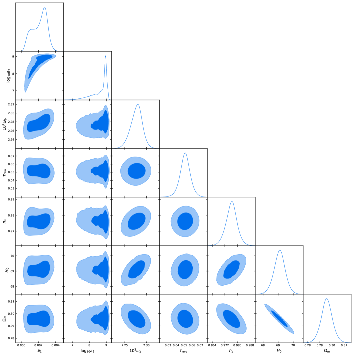
Figure 1: Marginalized two dimensional likelihoods for the kink model on fitting all chosen data sets (both early and late time ones).

The results for the one-dimensional 2$\sigma$ constraints are summarized in Table 3.

Parameters	95% limits
$a_{1}$	$0.0028_{{-}0.0023}^{{+}0.0006}$
$\log_{10}a_{2}$	$8.95_{{-}1.33}^{{+}0.20}$
$\log_{10}\beta$	${}<-3.5$
$10^{2}\omega_{b}$	$2.284_{{-}0.036}^{{+}0.019}$
$\tau_{{\rm reio}}$	$0.052_{{-}0.015}^{{+}0.013}$
$n_{s}$	$0.9778_{{-}0.0092}^{{+}0.0058}$
$H_{0}$	$69.19_{{-}0.90}^{{+}0.67}$
$\Omega_{m}$	$0.2952_{{-}0.0090}^{{+}0.0104}$

Table 3: One-dimensional 2$\sigma$ constraints for the cosmological parameters of interest obtained by fitting early times and late times data sets.

First of all, it is interesting to see the bound on $a_{1}$, which evidently states that $a_{1}$ is different from 0 at 2$\sigma$, i.e. the data suggests non-negligible deviation from $\Lambda$CDM. The bound on $a_{2}$ is also interesting as we have a lower and an upper limit. In particular, the value of $a_{2}$ selects the energy at which $f_{,CC}$ changes significantly. We will comment later on at which redshift this change occurs. Finally let us briefly discuss about the parameter $\beta$, which has been defined above as $a_{3}=\beta\,a_{2}$. The value of $\beta$ does not affect the value of the $\chi^{2}$ when it is sufficiently small. In fact, in order to study better the dependence of the $\chi^{2}$ on the parameter $\beta$, we have performed the experiment of changing the value of $\beta$ for the best fit and confirmed that its value does not affect the minimum of $\chi^{2}$, as shown in Fig. 2 which plots the behavior of the likelihood when $\beta$ varies, as long as $\log_{10}\beta\apprle-4.1$, for higher precision.

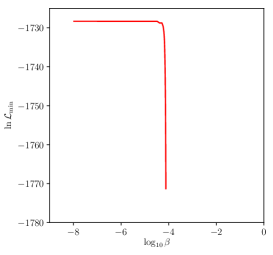
Figure 2: Independence of $\ln\text{$\mathcal{L}$}_{\text{min}}$ on $\beta$.

This means that we have a degeneracy for small values of $\beta$. In fact, the allowed lower bound was hitting the lower prior limit (which was set to be $10^{-9}$). Much smaller values would in fact require a sufficiently high precision which is not allowed in our computations. The meaning of a small $\beta$ is anyhow simple, the redshift range for which $f_{,CC}$ changes significantly cannot be too large, i.e. the transition between the two different $f_{,C}$ cannot be adiabatic. Later on, when we study in detail the minimum for the whole data sets, we will also try to understand the reason why large values of $\beta$ seem to be excluded.

As already stated above for these all-redshift-range data sets, we can see that the bestfit kink model alleviates the $H_{0}$ tension slightly, but, mostly, it gives a better fit on Planck data compared with $\Lambda$CDM. In fact, a value for $\Delta\chi^{2}=16.6$ is large enough (even on considering three more parameters for the kink model) as to exclude $\Lambda$CDM at 2$\sigma$ (because $a_{1}$ is different from 0 at 2$\sigma$, and the $a_{1}\to 0$ limit is a smooth one, as we have no other propagating mode than $\Lambda$CDM). This result is encouraging for the kink model and at least tells that flat-$\Lambda$CDM does not necessarily give the better fit to Planck data, or we may conclude that, if flat-$\Lambda$CDM is the only allowed model a priori, Planck data indicate some unknown systematics. A simple solution, in this sense following Occam’s razor, is that models different from $\Lambda$CDM have an arena to test gravity already in the Planck data sets and at high redshifts.

In summary, we have found a model which fits Planck data better than flat $\Lambda$CDM. The fact that there are models which fit Planck data better than flat $\Lambda$CDM is not new (see e.g. DiValentino:2019qzk ; DiValentino:2020hov ; Peirone:2019aua , the last one describing a model in the context of Horndeski theories). For example, it is now well known that Planck data prefer $\Omega_{K}\neq 0$ Aghanim:2018eyx ; DiValentino:2019qzk . However, a non-flat model is then in strong tension with BAO and inflationary paradigm at the same time DiValentino:2020hov . On the contrary, we have shown here that BAO data do not constrain much this model (or they constrain it as much as flat-$\Lambda$CDM) and, as a consequence, do not spoil the fact that the kink model still performs better than flat $\Lambda$CDM.

V.3 Background evolution

In the following we study in detail the behavior of the minimum of the $\chi^{2}$ starting with the background evolution. We have fixed the various background parameters to their bestfit values and integrated the background equations of motion. The results of the evolution of the three $\Omega_{i}$ functions are given in Fig. 3.

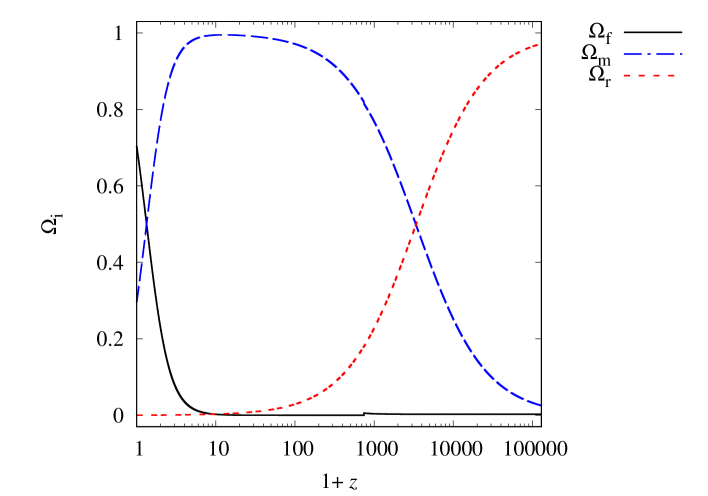
Figure 3: Evolution of the several $\Omega_{i}$ ($i=f,m,r$) functions during the evolution of the background for the bestfit kink model. Around $z\approx 743$ some non trivial behavior can be seen. Such a behavior will be studied more in detail in the following. The plot has been obtained on fixing $h=0.691867$, $\Omega_{m0}=0.2951803$, $a_{1}=2.766667\times 10^{-3}$, $\log_{10}a_{2}=8.949697$, $\log_{10}\beta=-4.5$, $\Omega_{f0}=0.7047323$.

We can see that some non-trivial dynamics happens at intermediate redshifts ($z\simeq 743$). In order to understand better what happens we further study the dynamics of the background for several variables. One variable of interest is $\varepsilon_{H}\equiv-\dot{H}/(NH^{2})$ (which can be calculated via Eq. (44)), as it shows whether the universe accelerates (when $\varepsilon_{H}<1$), decelerates (approaching 2 during radiation domination), and if some non-trivial singularity is present (besides the big-bang). In Fig. 4, we can see that around $z\simeq 743$, there is a fast but smooth transition at which $\varepsilon_{H}$ grows but remains finite. Therefore no singularity is present. Furthermore, we can see that this behavior takes place in an interval $\Delta z<1$. Finally this variable shows that the universe starts being radiation dominated, then matter dominated, and finally the universe starts accelerating.

(a) Evolution of $\epsilon_{H}$

(b) Evolution of $\epsilon_{H}$ (zoomed version)

Figure 4: Dynamics of the background variable $\varepsilon_{H}=-\dot{H}/(NH^{2})$. On the left panel we can see that today the universe accelerates (since $\varepsilon_{H}<1$), whereas at early times the universe is radiation dominated (as $\varepsilon_{H}\to 2$). On the right panel, we zoom around the redshift $z\simeq 743$, and we show that the transition is fast but smooth, i.e. no singularity is present (and this also implies that numerics are stable).

Another variable of interest is represented by $w_{f}=p_{f}/\rho_{f}$, i.e. the effective equation of state for the $f$-component. Its behavior is shown in Fig. 5, where we can see that the $f$-component, as already mentioned before, behaves as radiation at early times, but as a cosmological constant at late times.

(a) Evolution of $w_{f}$

(b) Evolution of $w_{f}$ (zoomed version)

Figure 5: Dynamics of the equation of state variable $w_{f}$ for the $f$-component. On the left panel we can see that today the universe tends to be dominated by a cosmological constant (since $w_{f}\approx-1$), whereas at early times the $f$-component tends to behave as a radiation-component as $w_{f}\approx 1/3$. On the right panel, we zoom around the redshift $z\simeq 743$, and we show that also for $w_{f}$ the transition is fast and smooth.

V.4 Evolution of the perturbations

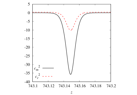
(a) Evolution of $c_{s}^{2}$ around the transition point

(b) Evolution of $c_{T}^{2}$ around the transition point

Figure 6: Evolution of the squared speeds of propagation for the scalar-matter modes and tensor modes. On the left panel we can see that the squared speeds of propagation for both dust ($c_{m}^{2}$) and radiation ($c_{r}^{2}$) change, and their values become negative during the transition. For a short time gradient instabilities take place, but as we will see later on, it is not so catastrophic (because the transition is short enough) as to make the matter perturbations totally unstable. This implies that $\beta$ (the parameter which determines how fast the transition is) must be small enough so that the instability-era is negligible. On the right panel, we show instead that at early times the speed of tensor modes was not unity, but today it is indistinguishable from unity as to pass the multi-messenger constraints.

(a) Evolution of $\delta_{\gamma}$

(b) Evolution of $\delta_{\gamma}$ around the transition point

Figure 7: Dynamics of the perturbation variable $\delta_{\gamma}$, the photon energy density contrast. It is clear from both panels (the right one describing its evolution during the transition-era), that such a variable still evolves in a way similar to GR after this transition ends). For this plot we have used the same bestfit parameters of the background, and on top of that $\omega_{b}=0.02284032$, $\omega_{c}=0.1184566$, $\tau_{{\rm reio}}=0.05183895$, $\ln(10^{10}A_{s})=3.039270$, $n_{s}=0.9778259$, and, as for the size of the wave-vector, $k=0.1$ Mpc^-1 (to enhance the effect of the instability in the very short wavelengths, but still linear).

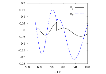
(a) Evolution of $\theta_{\gamma}$ and $\sigma_{\gamma}$

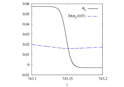
(b) Evolution of $\theta_{\gamma}$ and $\sigma_{\gamma}$ around the transition point

Figure 8: Dynamics of the perturbation variable $\theta_{\gamma}$, related to the photon velocity perturbation, and the photon shear $\sigma_{\gamma}$. For low redshifts, these variables become more and more negligible, as expected from their behaviors in GR. In the right panel, in order to enhance the change in the shear (with respect to the change of $\theta_{\gamma}$) we have multiplied its difference about the mean value at the transition era ($\approx 0.07$), by a factor of 20.

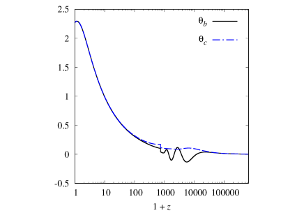
(a) Evolution of $\theta_{b}$ and $\theta_{c}$

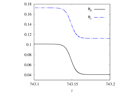
(b) Evolution of $\theta_{b}$ and $\theta_{c}$ around the transition point

Figure 9: Dynamics of the perturbation variables $\theta_{b}$ and $\theta_{c}$ (related to the velocity perturbations for the baryons and the CDM components respectively). Also for these variables, after the transition-era ends, their evolution is not too different from GR.

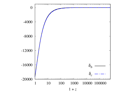
(a) Evolution of $\delta_{b}$ and $\delta_{c}$

(b) TT correlation dimensionless coefficients $C_{l}^{{\rm TT}}$, where any sudden transition has completely disappeared

Figure 10: Left panel: dynamics of the perturbation variables $\delta_{b}$ and $\delta_{c}$ (i.e. the density contrasts for baryons and CDM). Their evolution is dominated by the Jeans instability which leads to galaxy formation, in a way still consistent with GR. Right panel: TT correlation dimensionless coefficients $C_{l}^{{\rm TT}}$ which are bound by observations. This variable, involving typically an integral over the line of sight, smooths out the transition era for the perturbations.

After having studied in details the behavior of the background, we now focus on the dynamics of the perturbations. First of all, let us see what happens for the speed of propagation for the modes. In Fig. 6, we can see that the perturbation variables undergo an era of instability (because $c_{s}^{2}<0$), whereas tensor modes acquire a velocity of propagation different from unity (at early times, i.e. for $z>743$). The fact that there is an era of instability should make us worried, however such an era is relatively short. Therefore, there is the chance that the matter perturbations still remain finite after that transition-era ends. This is exactly what happens. After all, we already know that the $\chi^{2}$ is really good for this model. In fact, the $\chi^{2}$ from Planck comes from correlations of quantities (for example TT correlations) which typically involve an integral over the line-of-sight. Therefore, we expect that, if perturbations follow again GR evolution after the transition-era, the results for any such integral will be smooth. Since linear perturbations remains under control, one may expect a similar behavior for higher order perturbations, although we have not studied here this complicated issue.

Let us then study the evolution of the perturbation variables. As shown in Fig. 7, the photon energy density contrast $\delta_{\gamma}$ remains finite and once the transition is over, its evolution returns to the one similar to GR. Similar considerations can be made for the other perturbation variables, as shown in Figs. 8, 9 and 10.

To conclude the study of the best fit model, we want to emphasize again that the transition era is short-lived enough as to make the instability inefficient so that as soon as it ends, the dynamics is once again following the GR evolution. Therefore this model changes the $\chi^{2}$ not because of the transition, but because of the different behavior which it shows at early times (i.e. for $z>743$). It should be noticed that the numerics have been always stable as to be sensitive to small variations of $a_{1}$ (which on the bestfit is about ${+2}\times 10^{-3}$, whereas $a_{1}=0$ corresponds to $\Lambda$CDM) and of the parameter $\beta$ governing the duration of the transition era. This sensitivity has been achieved by reducing the standard tolerance parameters ($\simeq 10^{-5}$) which determine the precision of the numerical solution of the Boltzmann solver, CLASS, by about ten orders of magnitude.

VI Conclusion

We have studied a “kink model” within the class of minimally modified gravity theories dubbed $f(\mathcal{H})$ theories, which was shown in the present work to have a fit to several early times and late times data sets better than $\Lambda$CDM by $\Delta\chi^{2}=16.6$. We are impressed by several aspects of it. Most importantly, this model shows once for all that Planck data and $\Lambda$CDM do not fit so well with each other. In particular, the kink model performs better than $\Lambda$CDM especially on Planck 2018, but also on $H_{0}$ single-point data sets.

In the context of $\Lambda$CDM this aspect is ameliorated for Planck data alone notably if one introduces a non-zero curvature term, which however is not well motivated by inflation and moreover it is strongly suppressed by late time data (especially BAO). On the other hand, late time data do not strongly constrain the kink model, at most as much as flat-$\Lambda$CDM, and the kink model still keeps a better fit to Planck 2018 data.

On top of this consideration, the bestfit kink model is characterized by the presence of a transition era which happens at a redshift of $z\simeq 743$. Such a transition era happens at intermediate redshifts and not at very high energies. This means that there is the possibility that such a transition may occur in other contexts with strong gravity (inside a star for example). Furthermore during this transition era, the scalar perturbations have an instability ($c_{s}^{2}<0$) which, at least, as long as linear perturbation theory holds, does not seem to be catastrophic because of its short duration ($\Delta z\simeq 0.1$ around $z\simeq 743$) so that the matter perturbations (for which we have many constraints) do not show any divergent behavior. In particular, this transition era seems to be washed out when we look at observables which imply a line-of-sight integration.

The kink model then opens up an arena for modified gravity models, which so far are introduced mostly to address late time data only. This model in fact, addresses and resolves tension for $\Lambda$CDM in Planck data and at the same time shows a non-trivial window for phenomenology at intermediate redshifts. Future work is needed to address several points which remain to be explored, such as the existence, composition and evolution of compact objects for this model.

- [1] Arthur Kosowsky, Milos Milosavljevic, and Raul Jimenez. Efficient cosmological parameter estimation from microwave background anisotropies. Phys. Rev. D, 66:063007, 2002.
- [2] Ruth Durrer. The Cosmic Microwave Background. Cambridge University Press, Cambridge, 2008.
- [3] Jose Luis Bernal, Licia Verde, and Adam G. Riess. The trouble with . JCAP, 10:019, 2016.
- [4] Adam G. Riess, Stefano Casertano, Wenlong Yuan, Lucas M. Macri, and Dan Scolnic. Large Magellanic Cloud Cepheid Standards Provide a 1% Foundation for the Determination of the Hubble Constant and Stronger Evidence for Physics beyond CDM. Astrophys. J., 876(1):85, 2019.
- [5] Kenneth C. Wong et al. H0LiCOW XIII. A 2.4% measurement of from lensed quasars: tension between early and late-Universe probes. 2019.
- [6] M.J. Reid, J.A. Braatz, J.J. Condon, L.J. Greenhill, C. Henkel, and K.Y. Lo. The Megamaser Cosmology Project: I. VLBI observations of UGC 3789. Astrophys. J., 695:287–291, 2009.
- [7] Wendy L. Freedman et al. The Carnegie-Chicago Hubble Program. VIII. An Independent Determination of the Hubble Constant Based on the Tip of the Red Giant Branch. 7 2019.
- [8] Antonio De Felice, Chao-Qiang Geng, Masroor C. Pookkillath, and Lu Yin. Reducing the tension with generalized Proca theory. 2 2020.
- [9] Mario Ballardini, Matteo Braglia, Fabio Finelli, Daniela Paoletti, Alexei A. Starobinsky, and Caterina Umiltà. Scalar-tensor theories of gravity, neutrino physics, and the tension. 4 2020.
- [10] Matteo Braglia, Mario Ballardini, William T. Emond, Fabio Finelli, A. Emir Gumrukcuoglu, Kazuya Koyama, and Daniela Paoletti. A larger value for by an evolving gravitational constant. Phys. Rev. D, 102:023529, 2020.
- [11] Vivian Poulin, Tristan L. Smith, Tanvi Karwal, and Marc Kamionkowski. Early dark energy can resolve the hubble tension. Phys. Rev. Lett., 122:221301, Jun 2019.
- [12] Marika Asgari et al. KiDS+VIKING-450 and DES-Y1 combined: Mitigating baryon feedback uncertainty with COSEBIs. Astron. Astrophys., 634:A127, 2020.
- [13] Antonio De Felice and Shinji Mukohyama. Graviton mass might reduce tension between early and late time cosmological data. Phys. Rev. Lett., 118(9):091104, 2017.
- [14] Antonio De Felice, Shintaro Nakamura, and Shinji Tsujikawa. Suppressed cosmic growth in coupled vector-tensor theories. 4 2020.
- [15] Pavel Motloch and Wayne Hu. Tensions between direct measurements of the lens power spectrum from Planck data. Phys. Rev. D, 97(10):103536, 2018.
- [16] Pavel Motloch and Wayne Hu. Lensing-like tensions in the Planck legacy release. Phys. Rev. D, 101(8):083515, 2020.
- [17] Will Handley. Curvature tension: evidence for a closed universe. 8 2019.
- [18] Eleonora Di Valentino, Alessandro Melchiorri, and Joseph Silk. Planck evidence for a closed Universe and a possible crisis for cosmology. Nat. Astron., 4(2):196–203, 2019.
- [19] Eleonora Di Valentino, Alessandro Melchiorri, and Joseph Silk. Cosmic Discordance: Planck and luminosity distance data exclude LCDM. 3 2020.
- [20] N. Aghanim et al. Planck 2018 results. VI. Cosmological parameters. 7 2018.
- [21] Chunshan Lin and Shinji Mukohyama. A Class of Minimally Modified Gravity Theories. JCAP, 10:033, 2017.
- [22] Katsuki Aoki, Chunshan Lin, and Shinji Mukohyama. Novel matter coupling in general relativity via canonical transformation. Phys. Rev. D, 98(4):044022, 2018.
- [23] Katsuki Aoki, Antonio De Felice, Chunshan Lin, Shinji Mukohyama, and Michele Oliosi. Phenomenology in type-I minimally modified gravity. JCAP, 01:017, 2019.
- [24] Shinji Mukohyama and Karim Noui. Minimally Modified Gravity: a Hamiltonian Construction. JCAP, 07:049, 2019.
- [25] Antonio De Felice, Andreas Doll, and Shinji Mukohyama. A theory of type-II minimally modified gravity. 4 2020.
- [26] Antonio De Felice and Shinji Mukohyama. Minimal theory of massive gravity. Phys. Lett. B, 752:302–305, 2016.
- [27] Antonio De Felice and Shinji Mukohyama. Phenomenology in minimal theory of massive gravity. JCAP, 04:028, 2016.
- [28] Nadia Bolis, Antonio De Felice, and Shinji Mukohyama. Integrated Sachs-Wolfe-galaxy cross-correlation bounds on the two branches of the minimal theory of massive gravity. Phys. Rev. D, 98(2):024010, 2018.
- [29] Antonio De Felice, François Larrouturou, Shinji Mukohyama, and Michele Oliosi. Black holes and stars in the minimal theory of massive gravity. Phys. Rev. D, 98(10):104031, 2018.
- [30] Niayesh Afshordi, Daniel J.H. Chung, and Ghazal Geshnizjani. Cuscuton: A Causal Field Theory with an Infinite Speed of Sound. Phys. Rev. D, 75:083513, 2007.
- [31] Aya Iyonaga, Kazufumi Takahashi, and Tsutomu Kobayashi. Extended Cuscuton: Formulation. JCAP, 12:002, 2018.
- [32] Justin C. Feng and Sante Carloni. New class of generalized coupling theories. Phys. Rev. D, 101(6):064002, 2020.
- [33] Xian Gao and Zhi-Bang Yao. Spatially covariant gravity theories with two tensorial degrees of freedom: the formalism. Phys. Rev. D, 101(6):064018, 2020.
- [34] Katsuki Aoki, Mohammad Ali Gorji, and Shinji Mukohyama. A consistent theory of Einstein-Gauss-Bonnet gravity. 5 2020.
- [35] Raúl Carballo-Rubio, Francesco Di Filippo, and Stefano Liberati. Minimally modified theories of gravity: a playground for testing the uniqueness of general relativity. JCAP, 06:026, 2018. [Erratum: JCAP 11, E02 (2018)].
- [36] Diego Blas, Julien Lesgourgues, and Thomas Tram. The Cosmic Linear Anisotropy Solving System (CLASS) II: Approximation schemes. JCAP, 1107:034, 2011.
- [37] Masroor C. Pookkillath, Antonio De Felice, and Shinji Mukohyama. Baryon Physics and Tight Coupling Approximation in Boltzmann Codes. Universe, 6:6, 2020.
- [38] Thejs Brinckmann and Julien Lesgourgues. MontePython 3: boosted MCMC sampler and other features. Phys. Dark Univ., 24:100260, 2019.
- [39] Benjamin Audren, Julien Lesgourgues, Karim Benabed, and Simon Prunet. Conservative Constraints on Early Cosmology: an illustration of the Monte Python cosmological parameter inference code. JCAP, 1302:001, 2013.
- [40] N. Aghanim et al. Planck 2018 results. V. CMB power spectra and likelihoods. 2019.
- [41] Y. Akrami et al. Planck 2018 results. IX. Constraints on primordial non-Gaussianity. 2019.
- [42] Y. Akrami et al. Planck 2018 results. X. Constraints on inflation. 2018.
- [43] N. Aghanim et al. Planck 2018 results. VIII. Gravitational lensing. 2018.
- [44] Florian Beutler, Chris Blake, Matthew Colless, D. Heath Jones, Lister Staveley-Smith, Lachlan Campbell, Quentin Parker, Will Saunders, and Fred Watson. The 6dF Galaxy Survey: Baryon Acoustic Oscillations and the Local Hubble Constant. Mon. Not. Roy. Astron. Soc., 416:3017–3032, 2011.
- [45] Ashley J. Ross, Lado Samushia, Cullan Howlett, Will J. Percival, Angela Burden, and Marc Manera. The clustering of the SDSS DR7 main Galaxy sample – I. A 4 per cent distance measure at . Mon. Not. Roy. Astron. Soc., 449(1):835–847, 2015.
- [46] Shadab Alam et al. The clustering of galaxies in the completed SDSS-III Baryon Oscillation Spectroscopic Survey: cosmological analysis of the DR12 galaxy sample. Mon. Not. Roy. Astron. Soc., 470(3):2617–2652, 2017.
- [47] M. Betoule et al. Improved cosmological constraints from a joint analysis of the SDSS-II and SNLS supernova samples. Astron. Astrophys., 568:A22, 2014.
- [48] Antony Lewis. GetDist: a Python package for analysing Monte Carlo samples. 10 2019.
- [49] Chunshan Lin and Zygmunt Lalak. Novel matter coupling in einstein gravity.
- [50] Bernard F. Schutz. Perfect Fluids in General Relativity: Velocity Potentials and a Variational Principle. Phys. Rev., D2:2762–2773, 1970.
- [51] Bernard F. Schutz and Rafael Sorkin. Variational aspects of relativistic field theories, with application to perfect fluids. Annals Phys., 107:1–43, 1977.
- [52] J. David Brown. Action functionals for relativistic perfect fluids. Class. Quant. Grav., 10:1579–1606, 1993.
- [53] Antonio De Felice, Jean-Marc Gerard, and Teruaki Suyama. Cosmological perturbations of a perfect fluid and noncommutative variables. Phys. Rev., D81:063527, 2010.
- [54] B.P. Abbott et al. GW170817: Observation of Gravitational Waves from a Binary Neutron Star Inspiral. Phys. Rev. Lett., 119(16):161101, 2017.
- [55] Roberto Trotta. Bayes in the sky: Bayesian inference and model selection in cosmology. Contemp. Phys., 49:71–104, 2008.
- [56] Fabiola Arevalo, Antonella Cid, and Jorge Moya. AIC and BIC for cosmological interacting scenarios. Eur. Phys. J., C77(8):565, 2017.
- [57] Andrew R Liddle. Information criteria for astrophysical model selection. Mon. Not. Roy. Astron. Soc., 377:L74–L78, 2007.
- [58] Simone Peirone, Giampaolo Benevento, Noemi Frusciante, and Shinji Tsujikawa. Cosmological data favor Galileon ghost condensate over CDM. Phys. Rev. D, 100(6):063540, 2019.