Population Control meets Doob’s Martingale Theorems: the Noise-free Multimodal Case

Abstract.

We study a test-based population size adaptation (TBPSA) method, inspired from population control, in the noise-free multimodal case. In the noisy setting, TBPSA usually recommends, at the end of the run, the center of the Gaussian as an approximation of the optimum. We show that combined with a more naive recommendation, namely recommending the visited point which had the best fitness value so far, TBPSA is also powerful in the noise-free multimodal context. We demonstrate this experimentally and explore this mechanism theoretically: we prove that TBPSA is able to escape plateaus with probability one in spite of the fact that it can converge to local minima. This leads to an algorithm effective in the multimodal setting without resorting to a random restart from scratch.

1. Introduction

1.1. Population control

Population control has been proposed in (Hellwig and Beyer, 2016) and adapted in (Rapin and Teytaud, [n. d.]) under the name TBPSA (slightly different from the original population control) with great successes in noisy optimization. Consistently with (Astete-Morales et al., 2015), TBPSA breaks the barrier of a simple regret

(1) $$simple\ regret=O(1/\sqrt{number\ of\ evaluations}).$$

by doing steps in the recommendation smaller than the steps in the exploration; this is the so-called “mutate large, inherit small” paradigm (Beyer, 1998), i.e. we must explore “far” from the approximate optimum for reaching simple regret

(2) $$simple\ regret=O(1/number\ of\ evaluations).$$

1.2. Multimodal optimization

In the present paper we consider the application of the same approach to multimodal noise-free optimization. Multimodal optimization can be the search for a global optimum, in a context made difficult by the presence of many local optima. In other contexts, it refers to the search for diverse global optima. We show, in the case of a plateau, that though population control does not necessarily lead to large step-sizes it will nonetheless sample far thanks to a preserved diversity (i.e. no fast decrease of the step-size to zero) so that the increasing population will mechanically provide points far enough for escaping a local minimum.

1.3. Known Convergence Results

1.3.1. Convergence rate in the noise-free case.

It is known (Rechenberg, 1973; Beyer, 2001; Morinaga and Akimoto, 2019) that evolutionary algorithms converge in many cases to the optimum $x^{*}$ with rate $\log\|x_{n}-x^{*}\|=-\Omega(n)$.

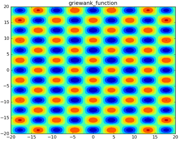
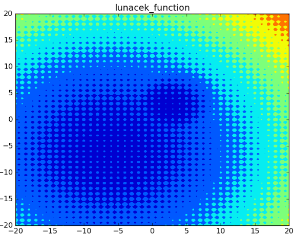
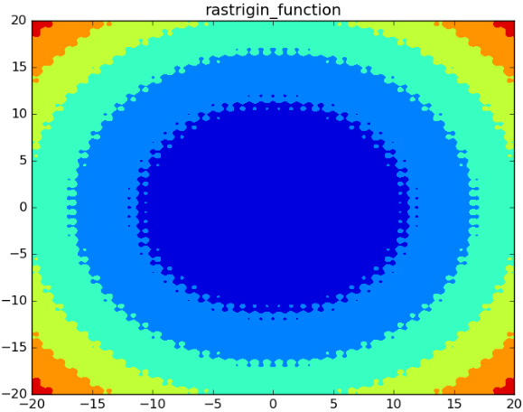
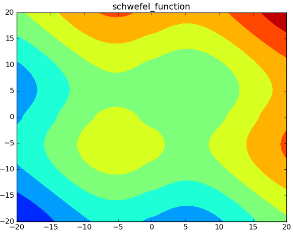
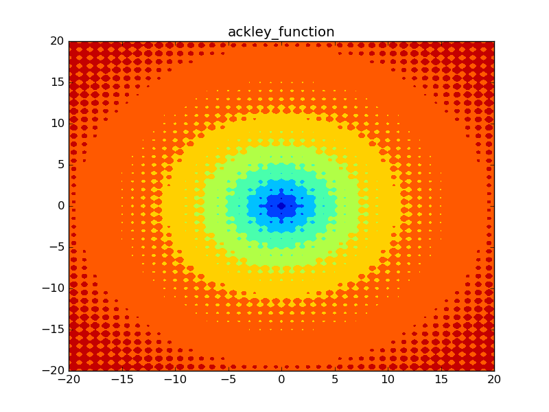
Figure 1. Level sets of some of our test functions. The optimum is in the bluest parts.

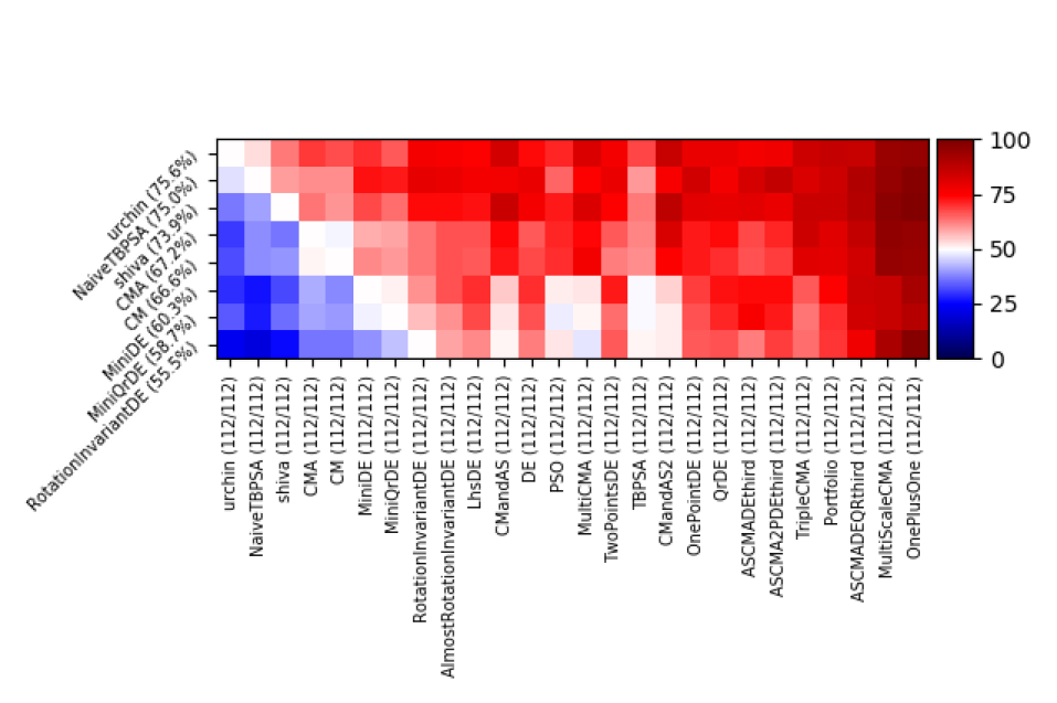
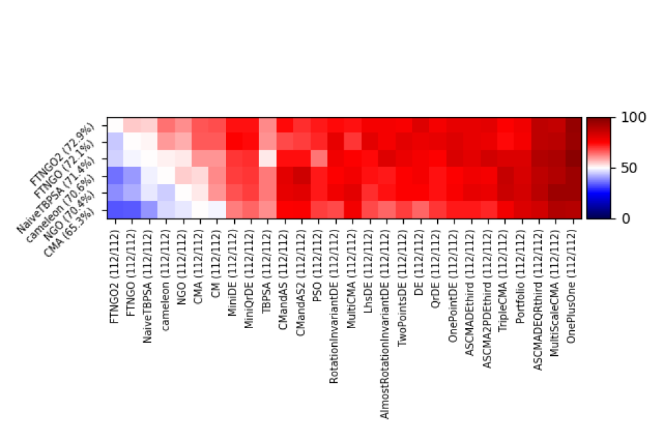
Figure 2. Parallel multimodal experiment in Nevergrad (termed “paramultimodal” in (Rapin and Teytaud, [n. d.])) at two distinct times: the list of algorithms varies, NaiveTBPSA performs well in both. Methods are ranked by score (best at the top row, best on the left hand side column). Only the best rows are presented. The score is the average frequency at which method $x$ outperformed other methods over instances of test functions. All other methods in the top (JNGO, FTNGO, cameleon, octopus, NGO, Shiva, Urchin) are combinations of algorithms based on algorithm selection: they incorporate our own method naiveTBPSA - all other methods are significantly weaker, CMA ranking best among methods not using NaiveTBPSA. This experiment considers 1000 concurrent function evaluations (parallelism), budget in $\{3000,10000,30000,100000\}$. We refer to (Rapin and Teytaud, [n. d.]) for a detailed description of all algorithms involved in the comparison and for the detailed setup. The objective functions are ”Hm”, ”Rastrigin”, ”Griewank”, ”Rosenbrock”, ”Ackley”, ”Lunacek”, ”DeceptiveMultimodal”, which are all either well known, or recent (namely Hm and DeceptiveMultimodal) but open sourced in (Rapin and Teytaud, [n. d.]).

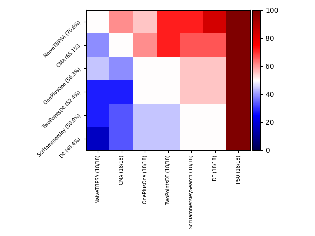
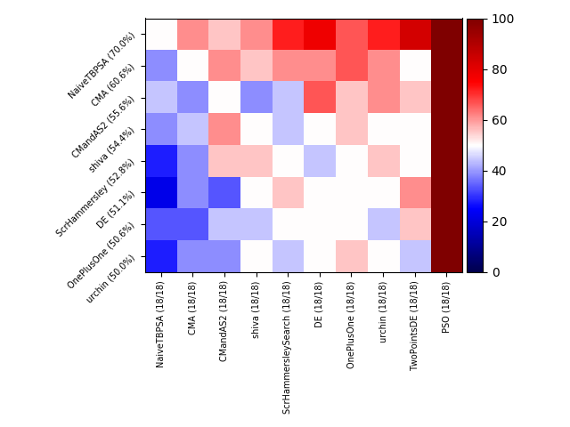
Figure 3. Parallel experiment in Nevergrad at two distinct dates with various algorithms present in that experiment at these distinct moments: this was not our goal, but we see that our code performs quite well in the parallel setting, in this experiment termed “parallel” (number of parallel evaluations equal to 20% of the budget, budget in $\{30,100,3000\}$, objective function in $\{Sphere,Rastrigin,Cigar\}$) and defined in (Rapin and Teytaud, [n. d.]).

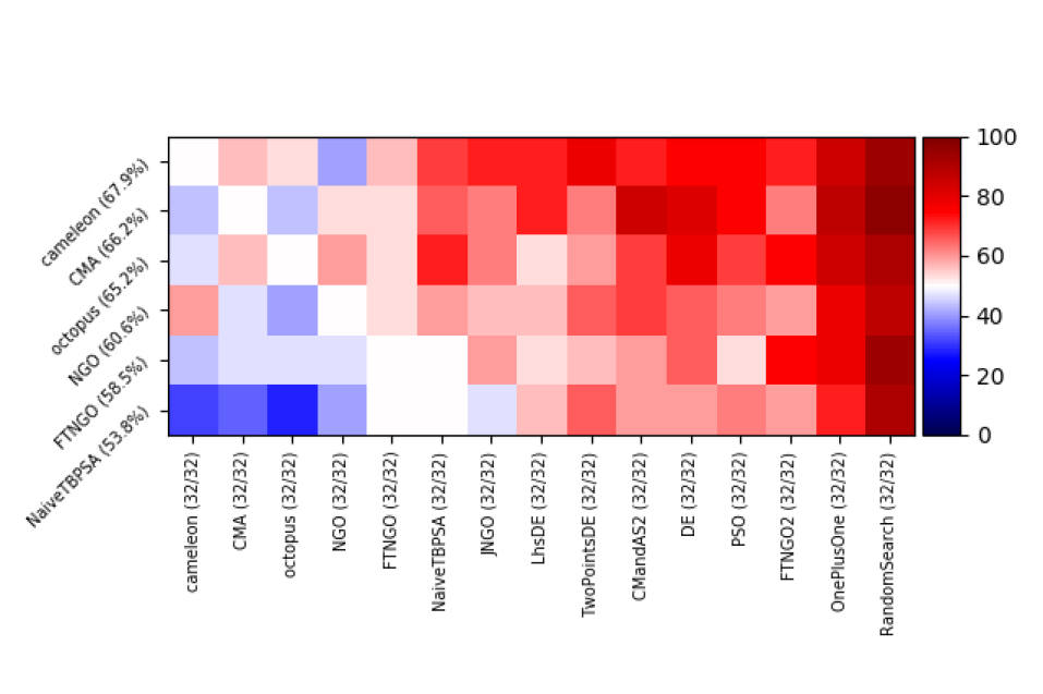
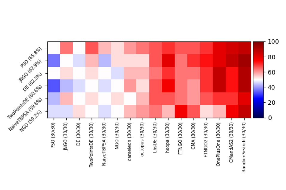
Figure 4. Multiobjective (top, set of problems with 2 or 3 objectives, budget from $100$ to $2900$, sequential or $100$ parallel workers) and Manyobjective (bottom, 6 objectives, budget from $100$ to $5900$, sequential or $100$ parallel workers) experiment in Nevergrad (code available in (Rapin and Teytaud, [n. d.])). This experiment uses the hypervolume indicator, i.e. the obtained method problem is multimodal. NaiveTBPSA performs better than PSO and all DE variants in the multiobjective case, but worse than CMA. It performs better than CMA and some variants of DE in the manyobjective case, but worse than some variants of DE and PSO. NaiveTBPSA has the best average rank over the two methods among simple methods. Algorithms such as Octopus, Cameleron, and names including “NGO” are combinations of algorithms designed independently of the present work: they are actually built on top of NaiveTBPSA and many others combined through an algorithm selection method.

1.3.2. Convergence in the multimodal case.

Multimodal optimization can be tackled in a number of ways (Casas, 2015). A wide research field in multimodal optimization consists in niching methods(Holland, 1975; Mahfoud, 1996), clearing(Petrowski, 1996), sharing(Goldberg and Richardson, 1987; Oliveto et al., 2019). As opposed to restart algorithms, these methods preserve diversity during the optimization run. At the cost of slower local convergence because of several local convergence runs simultaneously, these methods are more valuable when we want to find several optima (as opposed to just finding one of the global optima) or when we have to be parallel. For finding a single global optimum, restarts remain the method of choice and dominates e.g. (Hansen et al., 2012). When an algorithm stagnates, restart methods assume that it is stuck in a local optimum, and launches another run from a random initial point(Auger and Hansen, 2005). (Schoenauer et al., 2011) shows that quasi-random restarts are faster than random restarts. An improvement consists in adding a bandit for choosing between independent runs(Dubois et al., 2018). Theoretical investigations of restarts do exist. (Auger et al., 2005) shows that random diversification can be combined with evolution strategies for having both global convergence and reasonably fast rates. More precisely, it shows that a local linear convergence result, or a convergence faster than linear, is preserved when we use a random diversification: this combines the best of both worlds, almost sure convergence on a wide range of functions as in random search, and fast local convergence. This solution for multimodal convergence, however, is computationally expensive non-asymptotically as the multimodalities are handled through random search.

1.4. Optimization Algorithms

We present below TBPSA, the Test-Based Population-Size Adaptation method from (Rapin and Teytaud, [n. d.]). We will then present our counterpart, termed NaiveTBPSA, equipped with a different recommendation method. We also use many algorithms from (Rapin and Teytaud, [n. d.]) in our experiments. Readers unfamiliar with evolution strategies (ES) are referred to e.g. (Beyer, 2001).

1.4.1. TBPSA: population control for noise management.

We use a TBPSA self-adaptive $(\mu/\mu,\lambda)$-ES, implemented in Nevergrad, and strongly inspired from (Hellwig and Beyer, 2016). More precisely, each point is a pair $(x_{i},\sigma_{i})$ where $x_{i}$ is a candidate solution and the step-size $\sigma_{i}$ is a positive number. At each generation we compare their fitness values, select the $\mu$ best, average the selected candidates for choosing the next parent $x$, log-average their step-sizes for choosing the next parent step-size $\sigma$, and generate $\lambda$ points by $\sigma_{i}=\sigma\exp(\mathcal{N})$ and $x_{i}=x+\sigma_{i}\mathcal{N}_{d}$ for $1\leq i\leq\lambda$. Consistently with (Hellwig and Beyer, 2016), we multiply both $\lambda$ and $\mu$ by 2 if the $\lambda$ most recent and the $\lambda$ oldest out of the $5\lambda$ last points have no statistical difference. No statistical differnce means that the differences between averages is not 2 standard deviations apart - we multiply $\lambda$ and $\mu$ by $2^{-\frac{1}{4}}$ otherwise, without ever decreasing below the initial value or below the degree of parallelism requested by the application. Initialization: $\lambda=4d$, $\mu=d$, $\sigma=1/\sqrt{d}$. In classical applications of population control, this algorithm uses the last parent as a recommmendation. These two features (test-based population size, recommendation equal to the parent) are critical for reaching a convergence rate “simple regret $=O(1/\mbox{budget})$” rather than $1/\sqrt{\mbox{budget}}$ in the noisy case.

1.4.2. Naive TBPSA: TBPSA with best so far recommendation.

We define naiveTBPSA-$(\mu/\mu,\lambda)$-ES: the same as above, but using the same recommendation method as most algorithms in the noise-free context, namely the best visited point from the point of view of their fitness when visited.

2. Can we escape local minima ?

A key question for an optimization algorithm applied to multimodal objective functions is its ability to escape local minima. We distinguish two cases:

• Convex local optima for which the evolution strategy converges log-linearly. We show that adding an exponential increase of the population size is not enough for escaping such local optima.

• Plateaus. Then we show that the algorithm escapes plateaus, by stabilizing the step-size and increasing the population size.

2.1. Test-based population increase can not escape local minima if evolution strategies converge fast in this local optimum

Definition 2.1.

An algorithm $A$ is Gaussian-evolutionary if, with $\tau>0$, $\mathcal{N}_{n,i}$ a $d$-dimensional standard normal random variables and $\mathcal{N}^{\prime}_{n,i}$ a 1-dimensional standard normal random variable (all independent):

(3) $$\forall n,\lambda_{n} \leq M\lambda_{n-1}$$

(4) $$\forall n,i\leq\lambda_{n},\sigma_{n,i} = \sigma_{n}\exp(\tau\mathcal{N}^{\prime}_{n,i})$$

(5) $$\forall n,i\leq\lambda_{n},x_{n,i} = x_{n}+\sigma_{n,i}\mathcal{N}_{n,i}$$

$$\forall n,i\leq\lambda_{n},x_{n+1},\sigma_{n,i}\mbox{ and }\sigma_{n+1}$$ depend only on the

(6) $$(x_{n},\sigma_{n},(x_{n,i},\sigma_{n,i},f_{x_{n,i}})_{i\leq\lambda_{n}})$$

$\tau=0$ is possible and leads to a single step-size i.e. $\forall n,i,\sigma_{n,i}=\sigma_{n}$.

Definition 2.2.

We define a property $H1$ as follows:

$$H1(K):\forall n,||x_{n}||\leq K\mbox{ and }\sigma_{n,i}\leq K\exp(-n/K).$$

Property $H1$ means that the step size decreases exponentially and that points stay in a bounded set. Let us see why it is actually quite usual that $H1$ holds with some probability for some values of $K$. For the first part, namely the existence of $K$ such that $\forall n,||x_{n}||\leq K$, it is straightforward that it holds in the following case:

• an elitist strategy;

• a coercive objective function, i.e. $\forall K>0,\exists B,\forall x,||x||>B\Rightarrow f(x)>K$.

And for the second part, namely the exponential decrease of the step-size, (Auger and Hansen, 2013) and (Morinaga and Akimoto, 2019) show such an exponential convergence for wide ranges of functions.

Let us define a property of local convergence. This property will be used as an assumption in our results.

Definition 2.3.

An algorithm $A$ is locally convergent on a function $f$, denoted $LC(A,f)$ if

(7) $$\lim_{K\to\infty}P(H1(K))=1.$$

Remark: this is actually not a definition of convergence towards an optimum. This just means that we stay in a bounded neighborhood, and that the step-size decreases quickly. This is in fact a consequence of convergence, not a convergence. We just use this definition because it is weaker than a classical convergence to the optimum, and enough for our purpose. By using a weaker assumption, we strenghten our result; our theorem holds for this weak notion of local convergence, so a fortiori it holds for any stricter notion of local convergence.

Definition 2.4.

A Gaussian evolutionary algorithm approaches the optimum on an objective function $f$ if, almost surely, for all $\epsilon>0$, there is $n$ and $i\leq\lambda_{n}$ such that $\exists x^{*}\in\arg\min f,||x_{n}-x^{*}||\leq\epsilon\mbox{ or }||x_{n,i}-x^{*}||\leq\epsilon$.

Remarks:

• This definition could be extended to non-evolutionary or non-Gaussian algorithms.

• If an algorithm does not approach the optimum, then the hitting time, for sufficiently small precision, is infinite.

Theorem 2.5 (exponentially increasing the population size is not enough for escaping local minima).

Consider an algorithm such that Eqs 3-6 hold. We assume that for the fitness function $f$, $LC(A,f)$ holds. Then, for any $\epsilon>0$, there exists $K^{\prime}=K^{\prime}(\epsilon)>0$ such that with probability at least $1-\epsilon$, $\forall n,i,\ ||x_{n,i}||\leq K^{\prime}$.

This theorem can be rephrased as follows, for showing that it implies that we can not escape local minima.

Corollary 2.6 (Corollary of Theorem 2.5: a locally convergent Gaussian evolutionary algorithm does not escape local minima).

Consider $M\in{\mathbb{R}}$, and an algorithm $A$ such that Eqs 3-6 hold, and $LC(A,f)$.

Consider $\epsilon>0$. Let $K^{\prime}(\epsilon)$ be as in Theorem 2.5. Consider an objective function $g$ such that $\forall x\in B(0,K^{\prime}),g(x)=f(x)$ and $\arg\min g\not\in B(0,K^{\prime})$. Then, with probability at least $1-\epsilon$, none of the $x_{n,i}$ or the $x_{n}$ is outside $B(0,K^{\prime})$ and therefore the algorithm does not approach the optimum.

Proof of the theorem: Using Eq. 7, let us choose $K$ such that

(8) $$P(H1(K))>1-\epsilon/2.$$

Let us define $H2(K,K^{\prime})$, for $K^{\prime}>K$:

$$H2(K,K^{\prime}):\forall n>0,1\leq i\leq\lambda_{n},||{\mathcal{N}}_{n,i}||\leq\frac{K^{\prime}-K}{K}\exp(n/K)$$

$$\mbox{ where the }\mathcal{N}_{n,i}$$

are independent standard d-dimensional Gaussian random variables.

Algebra yields: $\forall K,K^{\prime}$,

if $$H1(K) H2(K,K^{\prime})$$ and ,

(9) then for all $$n,i ||x_{n,i}||\leq K^{\prime}$$ we have .

Using the bound $P(||\mathcal{N}_{n,i}||<t)\geq 1-\alpha\exp(-\beta t)$ for some $\alpha>0$ and $\beta>0$ and $t_{n}=\frac{K^{\prime}-K}{K}\exp(\frac{n}{K})$, we get $P(\sup_{i\leq\lambda_{n}}||\mathcal{N}_{n,i}||<t_{n})$

$$\geq 1-\alpha\lambda_{0}M^{n}\exp(-\beta t_{n})\mbox{ using Eq. \ref{e1}}$$

$$\geq 1-\alpha\lambda_{0}\exp\left(n\log(M)-\beta\frac{K^{\prime}-K}{K}\exp(\frac{n}{K})\right)$$

i.e. $P(\forall n,\sup_{i\leq\lambda_{n}}||\mathcal{N}_{n,i}||<t_{n})$

$$\geq 1-\alpha\lambda_{0}\sum_{n}\exp\left(n\log(M)-\beta\frac{K^{\prime}-K}{K}\exp(\frac{n}{K})\right).$$

For $K^{\prime}$ large enough, the right hand side is arbitrarily close to $1$. So we get:

(10) $$\forall\epsilon,\exists h:{\mathbb{R}}\to{\mathbb{R}},P(H2(K,K^{\prime}))\geq 1-\epsilon/2\mbox{ if }K^{\prime}>h(K).$$

Then, for such $K$ and $K^{\prime}$, the probability that none of the $x_{n,i}$ verifies $||x_{n,i}||>K^{\prime}$ is

$$\geq P(H2(K,K^{\prime})\mbox{ and }H1(K))\mbox{ by Eq.\ref{lm2}}$$

$$\geq 1-\epsilon/2+P(H1(K))-1\mbox{ by Eq. \ref{lm3}}$$

$$\geq 1-\epsilon/2+(1-\epsilon/2)-1\mbox{ by Eq. \ref{lm1}}$$

$$\geq 1-\epsilon$$

hence the expected result.

2.2. Test-based population increase can escape plateaus

There are several solutions for escaping plateaus:

• increasing the step-size;

• maintaining the diversity, i.e. ensuring that the step-size does not decrease to zero;

• adding random diversification over the domain as in (Auger et al., 2005).

We show below that TBPSA successfully escapes plateaus by maintaining the diversity.

We consider the following algorithm, directly inspired (though not completely equal) from (Hellwig and Beyer, 2016):

(11) $$s_{n,i} = \exp(\mathcal{N})$$

(12) $$\sigma_{n,i} = \sigma_{n}s_{n,i}$$

(13) $$z_{n,i} = \mathcal{N}_{d}$$

(14) $$x_{n,i} = x_{n}+\sigma_{n,i}z_{n,i}$$

(15) $$y_{n,i} = fitness(x_{n,i})$$

(16) $$I=I_{n} = \mu y_{n,i}$$ indices of the best

(17) $$\sigma_{n+1} = \exp(\mbox{average of the $\log\sigma_{n,i}$ for $i\in I$})$$

where $i$, unless stated otherwise, ranges over $\{1,\dots,\lambda_{n}\}$ and $\mathcal{N}_{d}$ denotes an independent $d$-dimensional Gaussian standard random variable and $\mathcal{N}$ an independent Gaussian random variable.

We did not specify how $x_{n+1}$ is defined; our result is independent of this.

We assume randomly broken ties.

We assume $\mu/\lambda$ lower-bounded.

For convenience, let us note $z^{\prime}_{n,i}=\sigma_{n,i}z_{n,i}/\sigma_{n}$; $z^{\prime}_{n,i}$ is distributed as $\exp(\mathcal{N})\mathcal{N}_{d}$ and

(18) $$x_{n,i}=x_{n}+\sigma_{n}z^{\prime}_{n,i}.$$

Lemma 2.7.

In case of random selection, ${\mathbb{E}}\log\sigma_{n+1}={\mathbb{E}}\log\sigma_{n}$.

Proof: By Eqs. 12 and 17.

Lemma 2.8.

Let us assume that $\lambda$ is multiplied by $2$ at each iteration and let us assume random selection. Then the supremum over $n$ of the variance of $\log\sigma_{n+1}$ is finite.

Proof: Eq 17 is an average over $\lambda$ independent points, $\lambda$ increases exponentially with the iteration index $n$, so the variance of $\log\sigma_{n+1}$ is the variance of $\log\sigma_{n}$ plus $Var(\mathcal{N})/2^{n}$ hence $Var(\log(\sigma_{n}))+1/2^{n}$. The total variance is therefore bounded by $2$.

Lemma 2.9.

With probability $1$, $\log\sigma_{n}$ converges to a finite limit $\log\sigma^{*}$.

Proof: By Doob’s first martingale theorem (Wikipedia contributors, 2019), using Lemmas 2.7 and 2.8.

Lemma 2.10.

With probability $1$, $\sup_{n\leq N}\sup_{i\leq\lambda_{n}}||x_{n,i}-x_{n}||$ goes to infinity as $N\to\infty$.

Proof: With probability $1$, $\sigma_{n}$ converges to a finite limit (by Lemma 2.9) and the supremum of the $z^{\prime}_{n,i}$ for $n\leq N,i\leq\lambda_{n}$ converges to infinity as $N\to\infty$; so Eq. 18 concludes.

Theorem 2.11.

Define $S$ a subset of the domain on which $f$ is constant. Then with probability $1$, there exists $n>0,i\leq\lambda_{n}$ such that either $x_{n}\not\in S$ or $x_{n,i}\not\in S$.

Proof: Consider $E_{N}$ the event “for all $n<N$ and $i$, $x_{n}$ and $x_{n,i}$ are all in $S$”. We have two random components:

• the $z_{n,i}$ and $s_{n,i}$;

• a random ranking, used for breaking ties.

As often done in theoretical analyses, we consider what would happen if the ranking was random instead of being based on the objective function. This corresponds to the case of random selection, i.e. plateaus and randomly broken ties.

Let us consider $x^{\prime}_{n}$ and $x^{\prime}_{n,i}$, counterpart, for the random selection case, of $x_{n}$ and $x_{n,i}$. Then, $x_{n},x^{\prime}_{n},x_{n,i},x^{\prime}_{n,i}$ live in the same domain and are defined for the same universe. We then consider $E_{rs,N}$, which is $E_{N}$ under random selection (using $x^{\prime}$ instead of $x$). And we consider $E_{f,N}$, which is $E_{N}$ under selection with $f$. First, consider $x_{n}$ and $x_{n,i}$ under random selection. $f$ has no impact on what is going on. Then, Lemma 2.10 applies. Therefore, with probability $1$, there is $n_{0}$ and $i_{0}$ such that $||x^{\prime}_{n_{0},i_{0}}-x^{\prime}_{n_{0}}||>diameter(S)$. This implies that

(19) $$P(\cap_{N\geq 0}E_{rs,N})=0.$$

If $E_{f,N}$ holds, then for all $n\neq N$ and $i\leq\lambda_{n}$, the probability distribution of $(x_{n},(x_{n,i})_{i\leq\lambda_{n}})$ and $(x^{\prime}_{n},(x^{\prime}_{n,i})_{i\leq\lambda_{n}})$ coincide, if $E_{f,n}$ holds. This means that $E_{f,N}$ implies $E_{rs,N}$. In particular $P(E_{f,N})\leq P(E_{rs,N})$. This and Eq. 19 imply that $P(\cap_{N}E_{f,N})=0$.

3. Experimental results

Fig. 2 and 3 present results in the parallel multimodal and multimodal setting respectively. Fig. 4 presents results in the multiobjective and manyobjective setting of Nevergrad. These test cases correspond to the use of the hypervolume indicator for converting the multiobjective setting into the monoobjective case. Figure 1 presents some of our objective functions. The detailed experimental setup is the default one in (Rapin and Teytaud, [n. d.]), all the code is public.

4. Conclusion

We have shown mathematically that the test-based population-size adaptation from (Hellwig and Beyer, 2016) can be applied in other contexts, namely multimodal optimization, in which it escapes plateaus. It does not escape convex local minima, but experimentally finite machine precision is enough for naturally ensuring some kind of restart. The method can be applied to other optimization algorithms.

Further work

We got good results in parallel settings, with moderate numbers of iterations. Results are less satisfactory for cases with large budget. We guess that applying the same TBPSA mechanism on top of other algorithms (CMA, CMSA, DE, PSO) might be beneficial. A limited precision in the test might also facilitate the detection of convex local minima.

References

- (1)
- Astete-Morales et al. (2015) Sandra Astete-Morales, Marie-Liesse Cauwet, and Olivier Teytaud. 2015. Evolution Strategies with Additive Noise: A Convergence Rate Lower Bound. In Foundations of Genetic Algorithms (Foundations of Genetic Algorithms). ACM, Aberythswyth, United Kingdom, 76–84. https://hal.inria.fr/hal-01077625
- Auger and Hansen (2005) A. Auger and N. Hansen. 2005. A restart CMA evolution strategy with increasing population size. In The 2005 IEEE International Congress on Evolutionary Computation (CEC’05), B. McKay et al. (Eds.), Vol. 2. 1769–1776.
- Auger and Hansen (2013) Anne Auger and Nikolaus Hansen. 2013. Linear Convergence on Positively Homogeneous Functions of a Comparison Based Step-Size Adaptive Randomized Search: the (1+1) ES with Generalized One-fifth Success Rule. (Oct. 2013). https://hal.inria.fr/hal-00877161 working paper or preprint.
- Auger et al. (2005) Anne Auger, Marc Schoenauer, and Olivier Teytaud. 2005. Local and global order 3/2 convergence of a surrogate evolutionary algorithm. In Genetic and Evolutionary Computation Conference, GECCO 2005, Proceedings, Washington DC, USA, June 25-29, 2005, Hans-Georg Beyer and Una-May O’Reilly (Eds.). ACM, 857–864. https://doi.org/10.1145/1068009.1068154
- Beyer (2001) H.G. Beyer. 2001. The theory of evolution strategies. Springer, Berlin. http://books.google.com/books?id=8tbInLufkTMC
- Beyer (1998) Hans-Georg Beyer. 1998. Mutate large, but inherit small! On the analysis of rescaled mutations in ( )-ES with noisy fitness data. In Parallel Problem Solving from Nature — PPSN V, Agoston E. Eiben, Thomas Bäck, Marc Schoenauer, and Hans-Paul Schwefel (Eds.). Springer Berlin Heidelberg, Berlin, Heidelberg, 109–118.
- Casas (2015) Noe Casas. 2015. Genetic Algorithms for multimodal optimization: a review. (2015). arXiv:cs.NE/1508.05342
- Dubois et al. (2018) Amaury Dubois, Julien Dehos, and Fabien Teytaud. 2018. Improving Multi-Modal Optimization Restart Strategy Through Multi-Armed Bandit. In IEEE ICMLA 2018 : 17th IEEE International Conference On Machine Learning And Applications. orlando, United States. https://hal.archives-ouvertes.fr/hal-02014193
- Goldberg and Richardson (1987) David E. Goldberg and Jon Richardson. 1987. Genetic Algorithms with Sharing for Multimodal Function Optimization. In Proceedings of the Second International Conference on Genetic Algorithms on Genetic Algorithms and Their Application. L. Erlbaum Associates Inc., USA, 41–49.
- Hansen et al. (2012) Nikolaus Hansen, Anne Auger, Steffen Finck, and Raymond Ros. 2012. Real-Parameter Black-Box Optimization Benchmarking: Experimental Setup. Technical Report. Université Paris Sud, INRIA Futurs, Équipe TAO, Orsay, France. http://coco.lri.fr/BBOB-downloads/download11.05/bbobdocexperiment.pdf
- Hellwig and Beyer (2016) Michael Hellwig and Hans-Georg Beyer. 2016. Evolution Under Strong Noise: A Self-Adaptive Evolution Strategy Can Reach the Lower Performance Bound - The pcCMSA-ES. In Parallel Problem Solving from Nature – PPSN XIV, Julia Handl, Emma Hart, Peter R. Lewis, Manuel López-Ibáñez, Gabriela Ochoa, and Ben Paechter (Eds.). Springer International Publishing, Cham, 26–36.
- Holland (1975) John H. Holland. 1975. Adaptation in Natural and Artificial Systems. University of Michigan Press.
- Mahfoud (1996) Samir W. Mahfoud. 1996. Niching Methods for Genetic Algorithms. Ph.D. Dissertation. USA.
- Morinaga and Akimoto (2019) Daiki Morinaga and Youhei Akimoto. 2019. Generalized drift analysis in continuous domain: linear convergence of (1 + 1)-ES on strongly convex functions with Lipschitz continuous gradients. In Proceedings of the 15th ACM/SIGEVO Conference on Foundations of Genetic Algorithms, FOGA 2019, Potsdam, Germany, August 27-29, 2019. 13–24. https://doi.org/10.1145/3299904.3340303
- Oliveto et al. (2019) Pietro S. Oliveto, Dirk Sudholt, and Christine Zarges. 2019. On the benefits and risks of using fitness sharing for multimodal optimisation. Theoretical Computer Science 773 (2019), 53 – 70. https://doi.org/10.1016/j.tcs.2018.07.007
- Petrowski (1996) A. Petrowski. 1996. A clearing procedure as a niching method for genetic algorithms. In Proceedings of IEEE International Conference on Evolutionary Computation. 798–803. https://doi.org/10.1109/ICEC.1996.542703
- Rapin and Teytaud ([n. d.]) J. Rapin and O. Teytaud. [n. d.]. Nevergrad - Gradient free optimization. https://github.com/facebookresearch/nevergrad/. ([n. d.]). Accessed: 2019-12-17.
- Rechenberg (1973) I. Rechenberg. 1973. Evolutionstrategie: Optimierung Technischer Systeme nach Prinzipien des Biologischen Evolution. Fromman-Holzboog Verlag, Stuttgart.
- Schoenauer et al. (2011) Marc Schoenauer, Fabien Teytaud, and Olivier Teytaud. 2011. Simple tools for multimodal optimization. In 13th Annual Genetic and Evolutionary Computation Conference, GECCO 2011, Companion Material Proceedings, Dublin, Ireland, July 12-16, 2011, Natalio Krasnogor and Pier Luca Lanzi (Eds.). ACM, 267–268. https://doi.org/10.1145/2001858.2002009
- Wikipedia contributors (2019) Wikipedia contributors. 2019. Doob’s martingale convergence theorem. (2019). https://en.wikipedia.org/wiki/Doob%27s_martingale_convergence_theorems#Doob’s_first_martingale_convergence_theorem [Online; accessed 22-July-2004].