Analysis of an infinite-buffer batch-size-dependent service queue with discrete-time Markovian arrival process: D-$MAP/G_{n}^{(a,b)}/1$

Abstract: Discrete-time queueing models find huge applications as they are used in modeling queueing systems arising in digital platforms like telecommunication systems, computer networks, etc. In this paper, we analyze an infinite-buffer queueing model with discrete Markovian arrival process. The units on arrival are served in batches by a single server according to the general bulk-service rule, and the service time follows general distribution with service rate depending on the size of the batch being served. We mathematically formulate the model using the supplementary variable technique and obtain the vector generating function at the departure epoch. The generating function is in turn used to extract the joint distribution of queue and server content in terms of the roots of the characteristic equation. Further, we develop the relationship between the distribution at the departure epoch and the distribution at arbitrary, pre-arrival and outside observer’s epoch, which is used to obtain the latter ones. We evaluate some essential performance measures of the system and also discuss the computing process extensively which is demonstrated by few numerical examples.
Keywords: Batch-size dependent, Discrete-time, General bulk service, Infinite-buffer, Markovian arrival process, Phase-type.

1 Introduction

Queueing models involving batch service have been investigated by many researchers in the past due to its potential application in several stochastic systems. Chaudhry and Templeton [11] and Medhi [18] provides a detailed discussion on different types of bulk queueing models. The general bulk service rule find application in the field of manufacturing and production systems, where the server starts service with a batch of minimum threshold size ‘$a$’ and a maximum size ‘$b$’. Moreover, the instances when the service rate (or service time) is dependent on the size of the batch being served, are more appropriate in modeling many of the real world problems. Such queues are known as batch size dependent service queues and plays a vital role in group screening practice of blood or urine samples examined for a particular disease, say HIV (see Abolnikov and Dukhovny [1], Bar-lev et al. [6, 5]). A group if found infected by the disease is set for further testing which may occur individually. If the size of the batch is large, then testing individual blood sample may take longer time which is a direct application to batch size dependent service. Moreover, in modern telecommunication systems, the transfer of information (data, voice, videos, images, etc.) occurs in packets in bulk where the transmission time depends on the batch size of packets. In the past few years many researchers have focussed on studying batch size dependent service queues, both with finite-buffer (see Yu and Alfa [24], Banerjee et al. [4]) and infinite-buffer (see Claeys et al. [12, 13], Pradhan and Gupta [20, 19]). Claeys et al. [13] provided the application of batch-size dependent service policy mainly in the area of telecommunication sector and illustrated the effect of neglecting batch-size dependent service times on the performance measures of the system.

In many real-world queueing systems the arrival of customers or units do not occur independently of each other. As for instance, in telecommunication systems the transmission of information, in the form of packetized data, takes place with a very high speed over a large network which exhibits burstiness, correlation and self-similarity. These features cannot be captured well using the traditional Poisson or Bernoulli arrival processes, and hence Markovian arrival process ($MAP$) can be adopted to cope with the bursty and correlated nature of the arrival process. In particular, the discrete-time analogous of $MAP$, i.e., D-$MAP$ is more applicable in telecommunication context due to the discrete nature of the transmission of information units in slotted systems, see for example Alfa [2, 3], Bruneel and Kim [7], Hunter [17], Takagi [22], Woodward [23]. D-$MAP$ is also a versatile arrival process and covers many other well known arrival processes such as the Bernoulli arrival process, the switched Bernoulli process (SBP), the Markov modulated Bernoulli process (MMBP), the discrete-time PH-renewal process etc. Much work has been done in the past on queueing models with D-$MAP$ arrival process with both finite and infinite-buffer. As for instance, Chaudhry and Gupta [9, 8] studied the finite-buffer D-$MAP/G/1/N$ and D-$MAP/G^{(a,b)}/1/N$ queue respectively where they obtained the queue-content distribution at various epochs. Further, Gupta et al [15] addressed a more general D-$MAP/G_{n}/1/N$ queue with the service time depending on the number of customers waiting in the queue. Yu and Alfa [24] considered a batch size dependent service D-${MAP/G^{(1,a,b)}_{n}/1/N}$ queue where the server serves the customers individually if there are less than ‘$a$’ customers in the queue, otherwise it servers according to the general bulk service ($a,b$) rule. For the infinite-buffer queue, Pradhan and Gupta [20] addressed the continuous-time $MAP/G^{(a,b)}_{n}/1$ queue whereas Claeys et al. [12] studied the discrete time analogous of [20] with the assumption of batch Markovian arrival process.

In this paper, we give a complete theoretical and computational analysis of an infinite-buffer discrete-time queueing model with Markovian arrival process (D-$MAP$). We assume that the server provides service in batches according to the general bulk service rule and the service time follows general distribution and depends on the size of the batch undergoing service. At first, using the supplementary variable technique, we obtain the steady-state bivariate vector generating function (VGF) of the queue-length and server content at the departure epoch of the batch, in a completely known form. From the bivariate VGF we extract the distribution at the departure epoch in terms of roots of the associated characteristic equation. Further, in order to obtain the distribution at arbitrary, pre-arrival and outside observer’s epoch, we establish their relation with the distribution at the departure epoch. Keeping note of the complexity of the model under consideration, we discuss in detail the whole computing process by considering discrete phase-type and arbitrary distributed service time distributions which cover almost all distributions that arise in various applications. We evaluate some significant performance characteristics of the model and demonstrate the computing process by certain numerical examples. In this paper, the use of supplementary variable technique makes the analysis of the model relatively simpler, which otherwise, would have been difficult using the embedded Markov chain technique because of the complexity associated with the construction of the transition probability matrix. It may be mentioned that Claeys et al. [12] considered the batch arrival D-$BMAP/G_{n}^{(l,c)}/1$ queue; however, they focussed mainly on obtaining the VGF and moments whereas in this paper we focus on extracting the distributions in a completely known form from the VGF.

The remaining portion of the paper is organized as follows. In Section 2 we give the detailed description of the considered discrete-time system followed by the analysis of the model in Section 3. In Section 4 we obtain the joint queue and server content distribution at various epochs and then discuss the computing process in detail in Section 5. In Section 6 we discuss some special cases of the model and evaluate some performance measures in Section 7. We present some numerical examples in Section 8 which is followed by the conclusion.

2 Model description, assumptions and notations

We consider a discrete-time queueing model in which the customers arrive according to discrete-Markovian arrival process(D-MAP) and service time of the batches of customers follow general distribution. Below we describe various processes.

• Arrival process: In D-MAP the arrivals are governed by an underlying $m$-state Markov chain having probability $C_{ij},(1\leq i,j\leq m)$ with a transition from state $i$ to $j$ without an arrival, and having probability $D_{ij},(1\leq i,j\leq m)$ with a transition from state $i$ to $j$ with an arrival. Let $\mathbf{C}=[C_{ij}],\mathbf{D}=[D_{ij}]$ be the $m\times m$ non-negative matrices both having at least one positive entry. The matrix $\mathbf{(C+D)}$ with $\mathbf{(C+D)}\boldsymbol{e}=\mbox{$\boldsymbol{e}$}$, where $\boldsymbol{e}$ is a column vector of ones with suitable dimension, is a stochastic matrix corresponding to an irreducible Markov chain underlying the D-MAP. Let $\overline{\mbox{\boldmath$\pi$}}=[\overline{\pi}_{1},\overline{\pi}_{2},\dots,\overline{\pi}_{m}]$ be the stationary probability vector of the underlying Markov chain, i.e., $\overline{\mbox{\boldmath$\pi$}}\mathbf{(C+D)}=\overline{\mbox{\boldmath$\pi$}},\leavevmode\nobreak\ \overline{\mbox{\boldmath$\pi$}}\mbox{$\boldsymbol{e}$}=1.$ The fundamental and stationary arrival rate is given by $(\lambda^{*})=\overline{\mbox{\boldmath$\pi$}}\mathbf{D}\mbox{$\boldsymbol{e}$}$.

• Service rule: A single server serves the customers in batches according to general bulk service $(a,b)$ rule. If the queue contains less than ‘$a$’ number of customers, server enters into the idle period and waits to initiate the service until at least ‘$a$’ customers gets accumulated. When the queue size is $r(a\leq r\leq b)$, entire group of customers are taken for service. However, if the queue size is greater than ‘$b$’, the server serves first ‘$b$’ customers and the remaining have to wait for the next round of service.

• Service process: The service time of the batches follow general distribution and are assumed to be dependent on batch size of ongoing service. Let us define the random variable ${V_{r}}(a\leq r\leq b)$ as the service time of a batch of size $r$ with probability mass function $s_{r}(n)=Pr(V_{r}=n),\leavevmode\nobreak\ n\geq 1$, probability generating function $S^{*}_{r}(z)=\sum\limits_{n=1}^{\infty}s_{r}(n)z^{n}$, and the mean service time $\mu^{-1}_{r}=S_{r}=\sum\limits_{n=1}^{\infty}ns_{r}(n)=S^{*(1)}_{r}(1)$, where $S^{*(1)}_{r}(1)=\frac{d}{dz}S^{*}_{r}(z)\Big{|}_{z=1}$.

• Late arrival system with delayed access: In discrete-time, the time axis is divided into intervals of equal length referred to as (time) slots, separated by slot boundaries. We assume that the length of each slot is unity and time axis is marked as $0,1,2,\dots,t,\dots$. We further assume that a potential arrival occurs in the interval $(t-,t)$ and a potential departure takes place in the interval $(t,t+)$. However, if an arrival finds the server idle, it cannot depart in the same slot in which it has arrived and has to wait for at least one slot before getting served. This is referred as late arrival system with delayed access (LAS-DA), see Hunter [17]. Various time epochs at which events occur are delineated in Figure 1.

• For the stability of the system, we must have that $\rho<1$ where $\rho=\frac{\lambda^{*}}{b\mu_{b}}$.

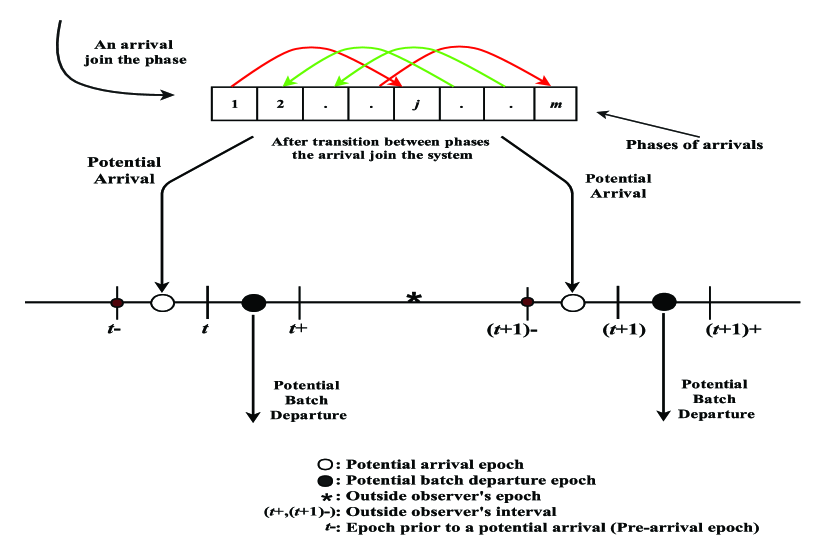
Figure 1: Various time epoch in LAS-DA

Let us denote the matrix $\mathbf{A}_{r}(n,k)$, $a\leq r\leq b,$ to be the matrix of order $m\times m$ whose $(i,j)$th element is the conditional probability that, a departure which left at least $a$ customers in the queue with the arrival process in state $i$, exactly $n$ new customers arrive during the service period (of length $k$ slots) of $r$ customers; the phase of the arrival process is in phase $j$ at the departure epoch. So $\mathbf{A}_{r}(n,k)$ can be written as

$$\mathbf{A}_{r}(0,k) = \mathbf{C}\mathbf{A}_{r}(0,k-1),\leavevmode\nobreak\ \leavevmode\nobreak\ k\geq 1,$$

$$\mathbf{A}_{r}(n,k) = \mathbf{C}\mathbf{A}_{r}(n,k-1)+\mathbf{D}\mathbf{A}_{r}(n-1,k-1),\leavevmode\nobreak\ \leavevmode\nobreak\ k\geq n\geq 1,$$

with $\mathbf{A}_{r}(0,0)=\mathbf{I}$ and $\mathbf{A}_{r}(n,k)=\mathbf{0},\leavevmode\nobreak\ n>k\geq 0,$ where $\mathbf{I}$ and $\mathbf{0}$ are identity and zero matrix of order $m\times m$, respectively. Also, let $\mathbf{A}^{*}_{r}(z,k)$ be the matrix-generating function of $\mathbf{A}_{r}(n,k)$, then

$$\mathbf{A}^{*}_{r}(z,k) = \sum_{n=0}^{\infty}\mathbf{A}_{r}(n,k)z^{n}=[\mathbf{A}^{*}_{r}(z,1)]^{k}=[\mathbf{C}+\mathbf{D}z]^{k},$$ (1)

where $\mathbf{A}^{*}_{r}(z,1)=\mathbf{C}+\mathbf{D}z$ is the matrix-generating function of the number of customers arriving in one slot. Let us denote the matrix $\mathbf{A}_{r}(n)=[A_{r}(n)]_{i,j}$, $n\geq 0,a\leq r\leq b,1\leq i,j\leq m,$ to be the conditional probability that, a departure which left at least $a$ customers in the queue with the arrival process in state $i$, and during the service period of $r$ customers exactly $n$ new customers arrive; the phase of the arrival process is in phase $j$ at the departure epoch. So $\mathbf{A}_{r}(n)$ can be written as

$$\mathbf{A}_{r}(n) = \sum_{k=\max(1,n)}^{\infty}s_{r}(k)\mathbf{A}_{r}(n,k),\leavevmode\nobreak\ \leavevmode\nobreak\ n\geq 0.$$

Further, let $\mathbf{A}^{*}_{r}(z)$ be the matrix-generating function of $\mathbf{A}_{r}(n)$. Therefore we have

$$\mathbf{A}^{*}_{r}(z) = \sum_{n=0}^{\infty}\mathbf{A}_{r}(n)z^{n}=\sum_{k=1}^{\infty}s_{r}(k)[\mathbf{C}+\mathbf{D}z]^{k},\leavevmode\nobreak\ \leavevmode\nobreak\ \leavevmode\nobreak\ \leavevmode\nobreak\ a\leq r\leq b.$$ (2)

Remark 1.

As and when more notations are used, they will be defined at respective places.

3 Analysis of the model

Let us define the following random variables at the beginning of the slot boundary $i.e.$ just before a potential arrival:

• $N_{q}(t-)\equiv$ Number of customers in the queue waiting for service at $t-$.

• $N_{s}(t-)\equiv$ Number of customers with the server at $t-$.

• $J(t-)\equiv$ Phase of the arrival process at $t-$.

• $U(t-)\equiv$ Remaining service time of a batch in service (if any) at $t-$.

Let us define for $1\leq i\leq m$,

$$p_{i}(n,0;t-) = Pr\{N_{q}(t-)=n,N_{s}(t-)=0,J(t-)=i,\hbox{server idle}\},\leavevmode\nobreak\ \leavevmode\nobreak\ \leavevmode\nobreak\ 0\leq n\leq a-1,$$

$$\pi_{i}(n,r,u;t-) = Pr\{N_{q}(t-)=n,N_{s}(t-)=r,J(t-)=i,U(t-)=u,\hbox{server busy}\},$$

$$\hskip 170.71652pt\leavevmode\nobreak\ n\geq 0,\leavevmode\nobreak\ a\leq r\leq b,\leavevmode\nobreak\ u\geq 1.$$

Also let us define the limiting probabilities as

$$p_{i}(n,0) = \lim_{t-\leavevmode\nobreak\ \rightarrow\infty}p_{i}(n,0;t-),$$

$$\pi_{i}(n,r,u) = \lim_{t-\leavevmode\nobreak\ \rightarrow\infty}\pi_{i}(n,r,u;t-).$$

Further, we define

$$\mbox{$\mathbf{p}$}(n,0) = [p_{1}(n,0),\dots,p_{i}(n,0),\dots,p_{m}(n,0)],$$

$$\mbox{\boldmath$\pi$}(n,r,u) = [\pi_{1}(n,r,u),\dots,\pi_{i}(n,r,u),\dots,\pi_{m}(n,r,u)].$$

Relating the states of the system at two consecutive time epochs $t-$ and $(t+1)-$ for each phase, and then using matrix and vector notations after taking $t-\leavevmode\nobreak\ \to\infty$, we obtain in steady-state

$$\mbox{$\mathbf{p}$}(0,0) = \mbox{$\mathbf{p}$}(0,0)\mathbf{C}+\sum_{r=a}^{b}\mbox{\boldmath$\pi$}(0,r,1)\mathbf{C},$$ (3)

$$\mbox{$\mathbf{p}$}(n,0) = \mbox{$\mathbf{p}$}(n,0)\mathbf{C}+\sum_{r=a}^{b}\mbox{\boldmath$\pi$}(n,r,1)\mathbf{C}+\mbox{$\mathbf{p}$}(n-1,0)\mathbf{D}+\sum_{r=a}^{b}\mbox{\boldmath$\pi$}(n-1,r,1)\mathbf{D},$$ (4)

$$\hskip 256.0748pt\leavevmode\nobreak\ \leavevmode\nobreak\ 1\leq n\leq a-1,$$

$$\mbox{\boldmath$\pi$}(0,a,u) = \mbox{\boldmath$\pi$}(0,a,u+1)\mathbf{C}+\mbox{$\mathbf{p}$}(a-1,0)\mathbf{D}s_{a}(u)+\sum_{r=a}^{b}\mbox{\boldmath$\pi$}(a,r,1)\mathbf{C}s_{a}(u)$$ (5)

$$\leavevmode\nobreak\ \leavevmode\nobreak\ +\sum_{r=a}^{b}\mbox{\boldmath$\pi$}(a-1,r,1)\mathbf{D}s_{a}(u),$$

$$\mbox{\boldmath$\pi$}(0,r,u) = \mbox{\boldmath$\pi$}(0,r,u+1)\mathbf{C}+\sum_{i=a}^{b}\mbox{\boldmath$\pi$}(r,i,1)\mathbf{C}s_{r}(u)+\sum_{i=a}^{b}\mbox{\boldmath$\pi$}(r-1,i,1)\mathbf{D}s_{r}(u),$$ (6)

$$\hskip 256.0748pt\leavevmode\nobreak\ \leavevmode\nobreak\ a+1\leq r\leq b,$$

$$\mbox{\boldmath$\pi$}(n,r,u) = \mbox{\boldmath$\pi$}(n,r,u+1)\mathbf{C}+\mbox{\boldmath$\pi$}(n-1,r,u+1)\mathbf{D},\leavevmode\nobreak\ \leavevmode\nobreak\ n\geq 1,\leavevmode\nobreak\ a\leq r\leq b-1,$$ (7)

$$\mbox{\boldmath$\pi$}(n,b,u) = \mbox{\boldmath$\pi$}(n,b,u+1)\mathbf{C}+\mbox{\boldmath$\pi$}(n-1,b,u+1)\mathbf{D}+\sum_{r=a}^{b}\mbox{\boldmath$\pi$}(n+b,r,1)\mathbf{C}s_{b}(u)$$ (8)

$$+\sum_{r=a}^{b}\mbox{\boldmath$\pi$}(n+b-1,r,1)\mathbf{D}s_{b}(u),\leavevmode\nobreak\ \leavevmode\nobreak\ n\geq 1.$$

Let us define the VGF of $\mbox{\boldmath$\pi$}(n,r,u)$ as

$$\mbox{\boldmath$\pi$}^{*}(n,r,z) = \sum_{u=1}^{\infty}\mbox{\boldmath$\pi$}(n,r,u)z^{u},\leavevmode\nobreak\ \leavevmode\nobreak\ \leavevmode\nobreak\ |z|\leq 1,\leavevmode\nobreak\ n\geq 0,\leavevmode\nobreak\ a\leq r\leq b.$$ (9)

It follows from (9) that

$$\mbox{\boldmath$\pi$}^{*}(n,r,1) = \sum_{u=1}^{\infty}\mbox{\boldmath$\pi$}(n,r,u)=\mbox{\boldmath$\pi$}(n,r),\leavevmode\nobreak\ \leavevmode\nobreak\ \leavevmode\nobreak\ \leavevmode\nobreak\ n\geq 0,\leavevmode\nobreak\ a\leq r\leq b.$$

Multiplying (5)-(8) by $z^{u}$ and summing over $u$ from 1 to $\infty$, we get

$$\mbox{\boldmath$\pi$}^{*}(0,a,z) = \frac{1}{z}(\mbox{\boldmath$\pi$}^{*}(0,a,z)-z\mbox{\boldmath$\pi$}(0,a,1))\mathbf{C}+\mbox{$\mathbf{p}$}(a-1,0)\mathbf{D}S^{*}_{a}(z)$$ (10)

$$+ \sum_{r=a}^{b}\mbox{\boldmath$\pi$}(a,r,1)\mathbf{C}S^{*}_{a}(z)+\sum_{r=a}^{b}\mbox{\boldmath$\pi$}(a-1,r,1)\mathbf{D}S^{*}_{a}(z),$$

$$\mbox{\boldmath$\pi$}^{*}(0,r,z) = \frac{1}{z}(\mbox{\boldmath$\pi$}^{*}(0,r,z)-z\mbox{\boldmath$\pi$}(0,r,1))\mathbf{C}+\sum_{i=a}^{b}\mbox{\boldmath$\pi$}(r,i,1)\mathbf{C}S^{*}_{r}(z)$$ (11)

$$+ \sum_{i=a}^{b}\mbox{\boldmath$\pi$}(r-1,i,1)\mathbf{D}S^{*}_{r}(z),\leavevmode\nobreak\ \leavevmode\nobreak\ a+1\leq r\leq b,$$

$$\mbox{\boldmath$\pi$}^{*}(n,r,z) = \frac{1}{z}(\mbox{\boldmath$\pi$}^{*}(n,r,z)-z\mbox{\boldmath$\pi$}(n,r,1))\mathbf{C}$$ (12)

$$+ \frac{1}{z}(\mbox{\boldmath$\pi$}^{*}(n-1,r,z)-z\mbox{\boldmath$\pi$}(n-1,r,1))\mathbf{D},\leavevmode\nobreak\ \leavevmode\nobreak\ n\geq 1,\leavevmode\nobreak\ a\leq r\leq b-1,$$

$$\mbox{\boldmath$\pi$}^{*}(n,b,z) = \frac{1}{z}(\mbox{\boldmath$\pi$}^{*}(n,b,z)-z\mbox{\boldmath$\pi$}(n,b,1))\mathbf{C}+\frac{1}{z}(\mbox{\boldmath$\pi$}^{*}(n-1,b,z)-z\mbox{\boldmath$\pi$}(n-1,b,1))\mathbf{D}$$ (13)

$$+ \sum_{r=a}^{b}\mbox{\boldmath$\pi$}(n+b,r,1)\mathbf{C}S^{*}_{b}(z)+\sum_{r=a}^{b}\mbox{\boldmath$\pi$}(n+b-1,r,1)\mathbf{D}S^{*}_{b}(z),\leavevmode\nobreak\ \leavevmode\nobreak\ n\geq 1.$$

Post multiplying by $\boldsymbol{e}$  in (3)-(4) and then summing over $n$ and $r$, we get

$$\mbox{$\mathbf{p}$}(a-1,0)\mathbf{D}\mbox{$\boldsymbol{e}$} = \sum_{n=0}^{a-2}\sum_{r=a}^{b}\mbox{\boldmath$\pi$}(n,r,1)\mbox{$\boldsymbol{e}$}+\sum_{r=a}^{b}\mbox{\boldmath$\pi$}(a-1,r,1)\mathbf{C}\mbox{$\boldsymbol{e}$}.$$ (14)

This can be written as

$$\mbox{$\mathbf{p}$}(a-1,0)\mathbf{D}\mbox{$\boldsymbol{e}$} = \sum_{n=0}^{a-1}\sum_{r=a}^{b}\mbox{\boldmath$\pi$}(n,r,1)\mathbf{C}\mbox{$\boldsymbol{e}$}+\sum_{n=0}^{a-2}\sum_{r=a}^{b}\mbox{\boldmath$\pi$}(n,r,1)\mathbf{D}\mbox{$\boldsymbol{e}$}.$$ (15)

Post multiplying (10)-(13) by $\boldsymbol{e}$  and then summing over $n$ and $r$, we get

$$\left(\frac{z-1}{z}\right)\sum_{n=0}^{\infty}\sum_{r=a}^{b}\mbox{\boldmath$\pi$}^{*}(n,r,z)\mbox{$\boldsymbol{e}$} = -\sum_{n=0}^{\infty}\sum_{r=a}^{b}\mbox{\boldmath$\pi$}(n,r,1)\mbox{$\boldsymbol{e}$}$$ (16)

$$+ \sum_{n=0}^{a-1}\sum_{r=a}^{b}\mbox{\boldmath$\pi$}(n,r,1)\mathbf{C}\mbox{$\boldsymbol{e}$}S^{*}_{a}(z)+\sum_{n=0}^{a-2}\sum_{r=a}^{b}\mbox{\boldmath$\pi$}(n,r,1)\mathbf{D}\mbox{$\boldsymbol{e}$}S^{*}_{a}(z)$$

$$+ \sum_{r=a}^{b}\mbox{\boldmath$\pi$}(a,r,1)\mathbf{C}\mbox{$\boldsymbol{e}$}S^{*}_{a}(z)+\sum_{r=a}^{b}\mbox{\boldmath$\pi$}(a-1,r,1)\mathbf{D}\mbox{$\boldsymbol{e}$}S^{*}_{a}(z),$$

$$+ \sum_{n=a+1}^{b}\sum_{r=a}^{b}\mbox{\boldmath$\pi$}(n,r,1)\mathbf{C}\mbox{$\boldsymbol{e}$}S^{*}_{n}(z)+\sum_{n=a}^{b-1}\sum_{r=a}^{b}\mbox{\boldmath$\pi$}(n,r,1)\mathbf{D}\mbox{$\boldsymbol{e}$}S^{*}_{n}(z)$$

$$+\sum_{n=b+1}^{\infty}\sum_{r=a}^{b}\mbox{\boldmath$\pi$}(n,r,1)\mathbf{C}\mbox{$\boldsymbol{e}$}S^{*}_{b}(z)+\sum_{n=b}^{\infty}\sum_{r=a}^{b}\mbox{\boldmath$\pi$}(n,r,1)\mathbf{D}\mbox{$\boldsymbol{e}$}S^{*}_{b}(z).$$

$$\Rightarrow\leavevmode\nobreak\ \leavevmode\nobreak\ \left(\frac{z-1}{z}\right)\sum_{n=0}^{\infty}\sum_{r=a}^{b}\mbox{\boldmath$\pi$}^{*}(n,r,z)\mbox{$\boldsymbol{e}$}$$ (17)

$$= \sum_{n=0}^{a}\sum_{r=a}^{b}\mbox{\boldmath$\pi$}(n,r,1)\mathbf{C}\mbox{$\boldsymbol{e}$}(S^{*}_{a}(z)-1)+\sum_{n=0}^{a-1}\sum_{r=a}^{b}\mbox{\boldmath$\pi$}(n,r,1)\mathbf{D}\mbox{$\boldsymbol{e}$}(S^{*}_{a}(z)-1)$$

$$+ \sum_{n=a+1}^{b}\sum_{r=a}^{b}\mbox{\boldmath$\pi$}(n,r,1)\mathbf{C}\mbox{$\boldsymbol{e}$}(S^{*}_{n}(z)-1)+\sum_{n=a}^{b-1}\sum_{r=a}^{b}\mbox{\boldmath$\pi$}(n,r,1)\mathbf{D}\mbox{$\boldsymbol{e}$}(S^{*}_{n}(z)-1)$$

$$+ \sum_{n=b+1}^{\infty}\sum_{r=a}^{b}\mbox{\boldmath$\pi$}(n,r,1)\mathbf{C}\mbox{$\boldsymbol{e}$}(S^{*}_{b}(z)-1)+\sum_{n=b}^{\infty}\sum_{r=a}^{b}\mbox{\boldmath$\pi$}(n,r,1)\mathbf{D}\mbox{$\boldsymbol{e}$}(S^{*}_{b}(z)-1).$$

Letting $z\rightarrow 1$ in (17), we get

$$1-\sum_{n=0}^{a-1}\mbox{$\mathbf{p}$}(n,0)\mbox{$\boldsymbol{e}$} = \sum_{n=0}^{a}\sum_{r=a}^{b}\mbox{\boldmath$\pi$}(n,r,1)\mbox{$\boldsymbol{e}$}S_{a}+\sum_{n=a+1}^{b}\sum_{r=a}^{b}\mbox{\boldmath$\pi$}(n,r,1)\mbox{$\boldsymbol{e}$}S_{n}$$ (18)

$$+ \sum_{n=b+1}^{\infty}\sum_{r=a}^{b}\mbox{\boldmath$\pi$}(n,r,1)\mbox{$\boldsymbol{e}$}S_{b}.$$

Further define

$$\widetilde{\mbox{\boldmath$\pi$}}^{*}(x,\xi,z) = \sum_{n=0}^{\infty}\sum_{r=a}^{b}\mbox{\boldmath$\pi$}^{*}(n,b,z)x^{n}\xi^{r},\leavevmode\nobreak\ \leavevmode\nobreak\ \leavevmode\nobreak\ |x|\leq 1,\leavevmode\nobreak\ |\xi|\leq 1,\leavevmode\nobreak\ |z|\leq 1.$$

Now we multiplying (10)-(13) by $x^{n}$ and $\xi^{r}$ and summing over $n$ from 0 to $\infty$ and $r$ from $a$ to $b$, we get

$$\widetilde{\mbox{\boldmath$\pi$}}^{*}(x,\xi,z)\left(\displaystyle{\frac{z\mathbf{I}-\mathbf{C}-\mathbf{D}x}{z}}\right) = -\sum_{n=0}^{\infty}\sum_{r=a}^{b}\mbox{\boldmath$\pi$}(n,r,1)x^{n}\xi^{r}(\mathbf{C}+\mathbf{D}x)+\mbox{$\mathbf{p}$}(a-1,0)\mathbf{D}\xi^{a}S^{*}_{a}(z)$$ (19)

$$+ \sum_{n=a}^{b}\sum_{r=a}^{b}(\mbox{\boldmath$\pi$}(n,r,1)\mathbf{C}+\mbox{\boldmath$\pi$}(n-1,r,1)\mathbf{D})\xi^{n}S^{*}_{n}(z)$$

$$+ \sum_{n=b+1}^{\infty}\sum_{r=a}^{b}(\mbox{\boldmath$\pi$}(n,r,1)\mathbf{C}+\mbox{\boldmath$\pi$}(n-1,r,1)\mathbf{D})x^{n-b}\xi^{b}S^{*}_{b}(z).$$

Our aim is to determine the bivariate VGF of the queue and server content. For this, we utilize the eigenvalues and eigenvectors of $(\mathbf{C+D}x)$, see Claeys et al [12], Pradhan and Gupta [20]. Now let $\gamma_{1}(x),\gamma_{2}(x),\dots,\gamma_{m}(x)$ are the eigenvalues and $\boldsymbol{\eta_{1}}(x),\boldsymbol{\eta_{2}}(x),\dots,\boldsymbol{\eta_{m}}(x)$ are the corresponding right eigenvectors of $(\mathbf{C+D}x)$. Thus, for $1\leq i\leq m$, we have

$$(\mathbf{C}+\mathbf{D}x)\boldsymbol{\eta_{i}}(x) = \gamma_{i}(x)\boldsymbol{\eta_{i}}(x),$$

$$\{\gamma_{i}(x)\mathbf{I}-(\mathbf{C}+\mathbf{D}x)\}\boldsymbol{\eta_{i}}(x) = \mathbf{0}.$$ (20)

Setting $z=\gamma_{i}(x)$ in (19) and post-multiplying it by $\boldsymbol{\eta_{i}}(x)$ on both sides and using (20), we get

$$\sum_{n=0}^{\infty}\sum_{r=a}^{b}\mbox{\boldmath$\pi$}(n,r,1)x^{n}\xi^{r}(\mathbf{C}+\mathbf{D}x)\boldsymbol{\eta_{i}}(x)$$ (21)

$$= \mbox{$\mathbf{p}$}(a-1,0)\mathbf{D}\xi^{a}S^{*}_{a}(\gamma_{i}(x))\boldsymbol{\eta_{i}}(x)$$

$$+ \sum_{n=a}^{b}\sum_{r=a}^{b}(\mbox{\boldmath$\pi$}(n,r,1)\mathbf{C}+\mbox{\boldmath$\pi$}(n-1,r,1)\mathbf{D})\xi^{n}S^{*}_{n}(\gamma_{i}(x))\boldsymbol{\eta_{i}}(x)$$

$$+ \sum_{n=b+1}^{\infty}\sum_{r=a}^{b}(\mbox{\boldmath$\pi$}(n,r,1)\mathbf{C}+\mbox{\boldmath$\pi$}(n-1,r,1)\mathbf{D})x^{n-b}\xi^{b}S^{*}_{b}(\gamma_{i}(x))\boldsymbol{\eta_{i}}(x).$$

Since (21) is true for all $i$ from 1 to $m$, so we have

$$\sum_{n=0}^{\infty}\sum_{r=a}^{b}\mbox{\boldmath$\pi$}(n,r,1)x^{n}\xi^{r}(\mathbf{C}+\mathbf{D}x)[\boldsymbol{\eta_{1}}(x),\dots,\boldsymbol{\eta_{m}}(x)]$$

$$=\mbox{$\mathbf{p}$}(a-1,0)\mathbf{D}\xi^{a}[S^{*}_{a}(\gamma_{1}(x))\boldsymbol{\eta_{1}}(x),\dots,S^{*}_{a}(\gamma_{m}(x))\boldsymbol{\eta_{m}}(x)]$$

$$+\sum_{n=a}^{b}\sum_{r=a}^{b}(\mbox{\boldmath$\pi$}(n,r,1)\mathbf{C}+\mbox{\boldmath$\pi$}(n-1,r,1)\mathbf{D})\xi^{n}[S^{*}_{n}(\gamma_{1}(x))\boldsymbol{\eta_{1}}(x),\dots,S^{*}_{n}(\gamma_{m}(x))\boldsymbol{\eta_{m}}(x)]$$

$$+\sum_{n=b+1}^{\infty}\sum_{r=a}^{b}(\mbox{\boldmath$\pi$}(n,r,1)\mathbf{C}+\mbox{\boldmath$\pi$}(n-1,r,1)\mathbf{D})x^{n-b}\xi^{b}[S^{*}_{b}(\gamma_{1}(x))\boldsymbol{\eta_{1}}(x),\dots,S^{*}_{b}(\gamma_{m}(x))\boldsymbol{\eta_{m}}(x)].$$ (22)

Further define

$$\mathbf{R}(x) = [\boldsymbol{\eta_{1}}(x),\boldsymbol{\eta_{2}}(x),\dots,\boldsymbol{\eta_{m}}(x)].$$ (23)

The inverse of $\mathbf{R}(x)$ exists whenever each eigenvalue is of multiplicity 1, for details see [12], [20]. Now using (23) in (22) and then post-multiplying it by $\mathbf{R}^{-1}(x)$, we get

$$\sum_{n=0}^{\infty}\sum_{r=a}^{b}\mbox{\boldmath$\pi$}(n,r,1)x^{n}\xi^{r}(\mathbf{C}+\mathbf{D}x)$$ (24)

$$= \mbox{$\mathbf{p}$}(a-1,0)\mathbf{D}\xi^{a}\mathbf{R}(x)[diag\{S^{*}_{a}(\gamma_{i}(x))\}_{i=1}^{m}]\mathbf{R}^{-1}(x)$$

$$+ \sum_{n=a}^{b}\sum_{r=a}^{b}(\mbox{\boldmath$\pi$}(n,r,1)\mathbf{C}+\mbox{\boldmath$\pi$}(n-1,r,1)\mathbf{D})\xi^{n}\mathbf{R}(x)[diag\{S^{*}_{n}(\gamma_{i}(x))\}_{i=1}^{m}]\mathbf{R}^{-1}(x)$$

$$+ \sum_{n=b+1}^{\infty}\sum_{r=a}^{b}(\mbox{\boldmath$\pi$}(n,r,1)\mathbf{C}+\mbox{\boldmath$\pi$}(n-1,r,1)\mathbf{D})x^{n-b}\xi^{b}\mathbf{R}(x)[diag\{S^{*}_{b}(\gamma_{i}(x))\}_{i=1}^{m}]\mathbf{R}^{-1}(x).$$

where $[diag\{S^{*}_{r}(\gamma_{i}(x))\}_{i=1}^{m}],\leavevmode\nobreak\ a\leq r\leq b$, is a diagonal matrix of order $m$ with diagonal entries $S^{*}_{r}(\gamma_{1}(x)),\dots,S^{*}_{r}(\gamma_{m}(x))$. Using the theory of eigenvalues and eigenvectors, we can write

$$\mathbf{C}+\mathbf{D}x = \mathbf{R}(x)[diag\{\gamma_{i}(x)\}_{i=1}^{m}]\mathbf{R}^{-1}(x),$$

$$\hbox{and\leavevmode\nobreak\ }\hskip 56.9055ptS^{*}_{r}(\mathbf{C}+\mathbf{D}x) = \mathbf{R}(x)[diag\{S^{*}_{r}(\gamma_{i}(x))\}_{i=1}^{m}]\mathbf{R}^{-1}(x).\hskip 113.81102pt$$ (25)

Now using (2) and (25) in (24), we obtain

$$\sum_{n=0}^{\infty}\sum_{r=a}^{b}\mbox{\boldmath$\pi$}(n,r,1)x^{n}\xi^{r}(\mathbf{C}+\mathbf{D}x) = \mbox{$\mathbf{p}$}(a-1,0)\mathbf{D}\xi^{a}\mathbf{A}^{*}_{a}(x)$$ (26)

$$+ \sum_{n=a}^{b}\sum_{r=a}^{b}(\mbox{\boldmath$\pi$}(n,r,1)\mathbf{C}+\mbox{\boldmath$\pi$}(n-1,r,1)\mathbf{D})\xi^{n}\mathbf{A}^{*}_{n}(x)$$

$$+ \sum_{n=b+1}^{\infty}\sum_{r=a}^{b}(\mbox{\boldmath$\pi$}(n,r,1)\mathbf{C}+\mbox{\boldmath$\pi$}(n-1,r,1)\mathbf{D})x^{n-b}\xi^{b}\mathbf{A}^{*}_{b}(x),$$

where $\mathbf{A}^{*}_{r}(x)=S^{*}_{r}(\mathbf{C}+\mathbf{D}x),\leavevmode\nobreak\ (a\leq r\leq b)$. Now using (26), we obtain the bivariate VGF of the queue-content at the departure epoch which is given in the next section.

3.1 Bivariate VGF at departure epoch

Let us define $\mbox{\boldmath$\pi$}^{+}(n,r)=[\pi_{1}^{+}(n,r),\pi_{2}^{+}(n,r),\dots,\pi_{m}^{+}(n,r)]$ as the joint probability vector whose $j$th element $(\pi_{j}^{+}(n,r))$ is the probability that there are $n$ number of customers in the queue at departure epoch of a batch of size $r$ and arrival process is in phase $j$.
$\mbox{\boldmath$\phi$}^{+}(n)$ = Probability vector that there are $n$ number of customers in the queue at departure epoch of a batch = $\sum\limits_{r=a}^{b}\mbox{\boldmath$\pi$}^{+}(n,r)$. Let us define $\widetilde{\mbox{\boldmath$\pi$}}^{+}(x,\xi)=\sum\limits_{n=0}^{\infty}\sum\limits_{r=a}^{b}\mbox{\boldmath$\pi$}^{+}(n,r)x^{n}\xi^{r},$ and $\mbox{\boldmath$\Phi$}^{+}(x)=\sum\limits_{n=0}^{\infty}\mbox{\boldmath$\phi$}^{+}(n)x^{n}$. Using probabilistic argument, $\mbox{\boldmath$\pi$}^{+}(n,r)$ and $\mbox{\boldmath$\pi$}(n,r,1)$ are connected as:

$$\mbox{\boldmath$\pi$}^{+}(0,r) = \Omega\mbox{\boldmath$\pi$}(0,r,1)\mathbf{C},$$ (27)

$$\mbox{\boldmath$\pi$}^{+}(n,r) = \Omega(\mbox{\boldmath$\pi$}(n,r,1)\mathbf{C}+\mbox{\boldmath$\pi$}(n-1,r,1)\mathbf{D}),\leavevmode\nobreak\ n\geq 1,\leavevmode\nobreak\ a\leq r\leq b.$$ (28)

where $\Omega^{-1}=\sum\limits_{n=0}^{\infty}\sum\limits_{r=a}^{b}\mbox{\boldmath$\pi$}(n,r,1)\mbox{$\boldsymbol{e}$}$.

Lemma 1.

$$\Omega^{-1} = \psi^{-1}\left(1-\sum_{n=0}^{a-1}\mbox{$\mathbf{p}$}(n,0)\mbox{$\boldsymbol{e}$}\right),$$

where $\psi=\sum\limits_{n=0}^{a}\mbox{\boldmath$\phi$}^{+}(n)\mbox{$\boldsymbol{e}$}S_{a}+\sum\limits_{n=a+1}^{b}\mbox{\boldmath$\phi$}^{+}(n)\mbox{$\boldsymbol{e}$}S_{n}+\sum\limits_{n=b+1}^{\infty}\mbox{\boldmath$\phi$}^{+}(n)\mbox{$\boldsymbol{e}$}S_{b}$.

Proof.

Equation (18) can be written as

$$1-\sum_{n=0}^{a-1}\mbox{$\mathbf{p}$}(n,0)\mbox{$\boldsymbol{e}$} = \sum_{r=a}^{b}\mbox{\boldmath$\pi$}(0,r,1)\mathbf{C}\mbox{$\boldsymbol{e}$}S_{a}$$

$$+ \sum_{n=1}^{a}\sum_{r=a}^{b}(\mbox{\boldmath$\pi$}(n,r,1)\mathbf{C}+\mbox{\boldmath$\pi$}(n-1,r,1)\mathbf{D})\mbox{$\boldsymbol{e}$}S_{a}$$

$$+ \sum_{n=a+1}^{b}\sum_{r=a}^{b}(\mbox{\boldmath$\pi$}(n,r,1)\mathbf{C}+\mbox{\boldmath$\pi$}(n-1,r,1)\mathbf{D})\mbox{$\boldsymbol{e}$}S_{n}$$

$$+ \sum_{n=b+1}^{\infty}\sum_{r=a}^{b}(\mbox{\boldmath$\pi$}(n,r,1)\mathbf{C}+\mbox{\boldmath$\pi$}(n-1,r,1)\mathbf{D})\mbox{$\boldsymbol{e}$}S_{b}.$$

Multiplying by $\Omega$ in above equation, we get

$$\Omega\left(1-\sum_{n=0}^{a-1}\mbox{$\mathbf{p}$}(n,0)\mbox{$\boldsymbol{e}$}\right) = \sum_{n=0}^{a}\mbox{\boldmath$\phi$}^{+}(n)\mbox{$\boldsymbol{e}$}S_{a}+\sum_{n=a+1}^{b}\mbox{\boldmath$\phi$}^{+}(n)\mbox{$\boldsymbol{e}$}S_{n}+\sum_{n=b+1}^{\infty}\mbox{\boldmath$\phi$}^{+}(n)\mbox{$\boldsymbol{e}$}S_{b}.$$

Hence proved. ∎

Lemma 2.

$$\Omega\mbox{$\mathbf{p}$}(a-1,0) = \sum_{n=0}^{a-1}\mbox{\boldmath$\phi$}^{+}(n)(\overline{\mathbf{D}})^{(a-1-n)}(\mathbf{I}-\mathbf{C})^{-1},$$

where $\overline{\mathbf{D}}=(\mathbf{I}-\mathbf{C})^{-1}\mathbf{D}$.

Proof.

Multiplying by $\Omega$ in (3), we get

$$\Omega\mbox{$\mathbf{p}$}(0,0)(\mathbf{I}-\mathbf{C}) = \mbox{\boldmath$\phi$}^{+}(0),$$

$$\Omega\mbox{$\mathbf{p}$}(0,0) = \mbox{\boldmath$\phi$}^{+}(0)(\mathbf{I}-\mathbf{C})^{-1},$$

Now multiplying by $\Omega$ in (4) for $n=i$ and after simplification, finally we get

$$\Omega\mbox{$\mathbf{p}$}(i,0)(\mathbf{I}-\mathbf{C}) = \sum_{n=0}^{i}\mbox{\boldmath$\phi$}^{+}(n)(\overline{\mathbf{D}})^{(i-n)},\leavevmode\nobreak\ \leavevmode\nobreak\ 1\leq i\leq a-1,$$

which gives

$$\Omega\mbox{$\mathbf{p}$}(a-1,0)(\mathbf{I}-\mathbf{C}) = \sum_{n=0}^{a-1}\mbox{\boldmath$\phi$}^{+}(n)(\overline{\mathbf{D}})^{(a-1-n)},$$

$$\Omega\mbox{$\mathbf{p}$}(a-1,0) = \sum_{n=0}^{a-1}\mbox{\boldmath$\phi$}^{+}(n)(\overline{\mathbf{D}})^{(a-1-n)}(\mathbf{I}-\mathbf{C})^{-1}.$$

Hence proved. ∎

Now multiplying (26) by $\Omega$ and using the definition of departure epoch probabilities and Lemma 1, we get

$$\widetilde{\mbox{\boldmath$\pi$}}^{+}(x,\xi)=\sum_{n=0}^{a-1}\mbox{\boldmath$\phi$}^{+}(n)(\overline{\mathbf{D}})^{(a-n)}\xi^{a}\mathbf{A}^{*}_{a}(x)+\sum_{n=a}^{b}\mbox{\boldmath$\phi$}^{+}(n)\xi^{n}\mathbf{A}^{*}_{n}(x)+\frac{\xi^{b}}{x^{b}}\sum_{n=b+1}^{\infty}\mbox{\boldmath$\phi$}^{+}(n)x^{n}\mathbf{A}^{*}_{b}(x).$$ (29)

Setting $\xi=1$ in (29), we get the VGF of $only$ queue length distribution $\mbox{\boldmath$\Phi$}^{+}(x)(=\widetilde{\mbox{\boldmath$\pi$}}^{+}(x,1))$ as

$$\mbox{\boldmath$\Phi$}^{+}(x)=\sum_{n=0}^{a-1}\mbox{\boldmath$\phi$}^{+}(n)(\overline{\mathbf{D}})^{(a-n)}\mathbf{A}^{*}_{a}(x)+\sum_{n=a}^{b}\mbox{\boldmath$\phi$}^{+}(n)\mathbf{A}^{*}_{n}(x)+\frac{1}{x^{b}}\sum_{n=b+1}^{\infty}\mbox{\boldmath$\phi$}^{+}(n)x^{n}\mathbf{A}^{*}_{b}(x),$$ (30)

which gives

$$\mbox{\boldmath$\Phi$}^{+}(x)(x^{b}\mathbf{I}-\mathbf{A}^{*}_{b}(x)) = \sum_{n=0}^{a-1}\mbox{\boldmath$\phi$}^{+}(n)\Big{(}(\overline{\mathbf{D}})^{(a-n)}x^{b}\mathbf{A}^{*}_{a}(x)-x^{n}\mathbf{A}^{*}_{b}(x)\Big{)}$$ (31)

$$+ \sum_{n=a}^{b-1}\mbox{\boldmath$\phi$}^{+}(n)\Big{(}x^{b}\mathbf{A}^{*}_{n}(x)-x^{n}\mathbf{A}^{*}_{b}(x)\Big{)}.$$

From (29), we have

$$\widetilde{\mbox{\boldmath$\pi$}}^{+}(x,\xi) = \sum_{n=0}^{a-1}\mbox{\boldmath$\phi$}^{+}(n)(\overline{\mathbf{D}})^{(a-n)}\xi^{a}\mathbf{A}^{*}_{a}(x)+\sum_{n=a}^{b}\mbox{\boldmath$\phi$}^{+}(n)\xi^{n}\mathbf{A}^{*}_{n}(x)$$ (32)

$$+ \frac{\xi^{b}}{x^{b}}\left(\mbox{\boldmath$\Phi$}^{+}(x)-\sum_{n=0}^{b}\mbox{\boldmath$\phi$}^{+}(n)x^{n}\right)\mathbf{A}^{*}_{b}(x).$$

Now substituting the value of the vector $\mbox{\boldmath$\Phi$}^{+}(x)$ from (31) to (32), we get

$$\widetilde{\mbox{\boldmath$\pi$}}^{+}(x,\xi) = \sum_{n=0}^{a-1}\mbox{\boldmath$\phi$}^{+}(n)(\overline{\mathbf{D}})^{(a-n)}\xi^{a}\mathbf{A}^{*}_{a}(x)+\sum_{n=a}^{b}\mbox{\boldmath$\phi$}^{+}(n)\xi^{n}\mathbf{A}^{*}_{n}(x)$$ (33)

$$+ \frac{\xi^{b}}{x^{b}}\Big{(}\Big{[}\sum_{n=0}^{a-1}\mbox{\boldmath$\phi$}^{+}(n)\Big{(}(\overline{\mathbf{D}})^{(a-n)}x^{b}\mathbf{A}^{*}_{a}(x)-x^{n}\mathbf{A}^{*}_{b}(x)\Big{)}$$

$$+ \sum_{n=a}^{b-1}\mbox{\boldmath$\phi$}^{+}(n)\Big{(}x^{b}\mathbf{A}^{*}_{n}(x)-x^{n}\mathbf{A}^{*}_{b}(x)\Big{)}\Big{]}(x^{b}\mathbf{I}-\mathbf{A}^{*}_{b}(x))^{-1}$$

$$- \sum_{n=0}^{b}\mbox{\boldmath$\phi$}^{+}(n)x^{n}\Big{)}\mathbf{A}^{*}_{b}(x).$$

Post multiplying by $(x^{b}\mathbf{I}-\mathbf{A}^{*}_{b}(x))$ on both sides of (33), we obtain

$$\widetilde{\mbox{\boldmath$\pi$}}^{+}(x,\xi) = \Bigg{(}\sum_{n=0}^{a-1}\mbox{\boldmath$\phi$}^{+}(n)\Big{(}(\xi^{b}-\xi^{a})(\overline{\mathbf{D}})^{(a-n)}\mathbf{A}^{*}_{a}(x)\mathbf{A}^{*}_{b}(x)+(\overline{\mathbf{D}})^{(a-n)}\xi^{a}x^{b}\mathbf{A}^{*}_{a}(x)-\xi^{b}x^{n}\mathbf{A}^{*}_{b}(x)\Big{)}$$

$$+ \sum_{n=a}^{b-1}\mbox{\boldmath$\phi$}^{+}(n)\Big{(}(\xi^{b}-\xi^{n})\mathbf{A}^{*}_{n}(x)\mathbf{A}^{*}_{b}(x)+\xi^{n}x^{b}\mathbf{A}^{*}_{n}(x)-\xi^{b}x^{n}\mathbf{A}^{*}_{b}(x)\Big{)}\Bigg{)}(x^{b}\mathbf{I}-\mathbf{A}^{*}_{b}(x))^{-1}.$$

4 Joint queue and server content distributions at various epochs

In this section, we obtain joint queue and server content distribution at arbitrary, pre-arrival and outside observer’s epochs.

4.1 Joint queue and server content distribution at arbitrary epoch

The joint distribution of queue and server content at arbitrary epoch plays an important role in obtaining system length distribution and also in evaluation of several key performance measures of the queueing model under consideration. The following theorem presents a correspondence between departure and arbitrary epoch probability vectors.

Theorem 1.

The steady-state probability vectors $\{\mbox{$\mathbf{p}$}(n,0),\mbox{\boldmath$\pi$}(n,r)\}$ and $\{\mbox{\boldmath$\pi$}^{+}(n,r),\mbox{\boldmath$\phi$}^{+}(n)\}$ are connected by

$$\mbox{$\mathbf{p}$}(n,0) = \Omega^{-1}\sum_{j=0}^{n}\mbox{\boldmath$\phi$}^{+}(j)(\overline{\mathbf{D}})^{(n-j)}(\mathbf{I}-\mathbf{C})^{-1},\leavevmode\nobreak\ \leavevmode\nobreak\ \leavevmode\nobreak\ 0\leq n\leq a-1,$$ (35)

$$\mbox{\boldmath$\pi$}(0,a) = \Big{(}\mbox{$\mathbf{p}$}(a-1,0)\mathbf{D}+\Omega^{-1}(\mbox{\boldmath$\phi$}^{+}(a)-\mbox{\boldmath$\pi$}^{+}(0,a))\Big{)}(\mathbf{I}-\mathbf{C})^{-1},$$ (36)

$$\mbox{\boldmath$\pi$}(0,r) = \Omega^{-1}(\mbox{\boldmath$\phi$}^{+}(r)-\mbox{\boldmath$\pi$}^{+}(0,r))(\mathbf{I}-\mathbf{C})^{-1},\leavevmode\nobreak\ \leavevmode\nobreak\ \leavevmode\nobreak\ \leavevmode\nobreak\ a+1\leq r\leq b,$$ (37)

$$\mbox{\boldmath$\pi$}(n,r) = \Big{(}\mbox{\boldmath$\pi$}(n-1,r)\mathbf{D}-\Omega^{-1}\mbox{\boldmath$\pi$}^{+}(n,r)\Big{)}(\mathbf{I}-\mathbf{C})^{-1},\leavevmode\nobreak\ \leavevmode\nobreak\ n\geq 1,\leavevmode\nobreak\ \leavevmode\nobreak\ a\leq r\leq b-1,$$ (38)

$$\mbox{\boldmath$\pi$}(n,b) = \Big{(}\mbox{\boldmath$\pi$}(n-1,b)\mathbf{D}+\Omega^{-1}(\mbox{\boldmath$\phi$}^{+}(n+b)-\mbox{\boldmath$\pi$}^{+}(n,b))\Big{)}(\mathbf{I}-\mathbf{C})^{-1},\leavevmode\nobreak\ \leavevmode\nobreak\ n\geq 1.$$ (39)

Proof.

From Lemma 2, we obtain (35). Now setting $z=1$ in (10)-(13), we get

$$\mbox{\boldmath$\pi$}(0,a)(\mathbf{I}-\mathbf{C}) = -\mbox{\boldmath$\pi$}(0,a,1)\mathbf{C}+\mbox{$\mathbf{p}$}(a-1,0)\mathbf{D}+\sum_{r=a}^{b}\mbox{\boldmath$\pi$}(a,r,1)\mathbf{C}+\sum_{r=a}^{b}\mbox{\boldmath$\pi$}(a-1,r,1)\mathbf{D},$$ (40)

$$\mbox{\boldmath$\pi$}(0,r)(\mathbf{I}-\mathbf{C}) = -\mbox{\boldmath$\pi$}(0,r,1)\mathbf{C}+\sum_{i=a}^{b}\mbox{\boldmath$\pi$}(r,i,1)\mathbf{C}+\sum_{i=a}^{b}\mbox{\boldmath$\pi$}(r-1,i,1)\mathbf{D},\leavevmode\nobreak\ \leavevmode\nobreak\ a+1\leq r\leq b,$$ (41)

$$\mbox{\boldmath$\pi$}(n,r)(\mathbf{I}-\mathbf{C}) = -\mbox{\boldmath$\pi$}(n,r,1)\mathbf{C}+(\mbox{\boldmath$\pi$}(n-1,r)-\mbox{\boldmath$\pi$}(n-1,r,1))\mathbf{D},\leavevmode\nobreak\ n\geq 1,\leavevmode\nobreak\ a\leq r\leq b-1,\leavevmode\nobreak\ \leavevmode\nobreak\$$ (42)

$$\mbox{\boldmath$\pi$}(n,b)(\mathbf{I}-\mathbf{C}) = -\mbox{\boldmath$\pi$}(n,b,1)\mathbf{C}+(\mbox{\boldmath$\pi$}(n-1,b)-\mbox{\boldmath$\pi$}(n-1,b,1))\mathbf{D}+\sum_{r=a}^{b}\mbox{\boldmath$\pi$}(n+b,r,1)\mathbf{C}$$ (43)

$$+ \sum_{r=a}^{b}\mbox{\boldmath$\pi$}(n+b-1,r,1)\mathbf{D},\leavevmode\nobreak\ n\geq 1.$$

Now multiplying (40)-(43) by $\Omega$ and using Lemma 1,2 and then using the definition of departure epoch, we get the required relation between arbitrary and departure epoch as given in (36)-(39). ∎

4.2 Queue length and server content distribution at pre-arrival epoch

Let $\mbox{$\mathbf{p}$}^{-}(n,0),\leavevmode\nobreak\ (0\leq n\leq a-1)$ and $\mbox{\boldmath$\pi$}^{-}(n,r),\leavevmode\nobreak\ (a\leq r\leq b,n\geq 0)$ be the $1\times m$ vectors with $i$th component as $p_{i}^{-}(n,0)$ and $\pi_{i}^{-}(n,r)$, respectively. Let us define $p_{i}^{-}(n,0)$ as the steady-state probability that an arrival find $n,\leavevmode\nobreak\ (0\leq n\leq a-1)$ customers in the queue, server idle, and phase of the arrival process is $i$. Similarly, we define $\pi_{i}^{-}(n,r)$ to be the steady-state probability that an arrival finds $n(\geq 0)$ customers in the queue, server busy with $r,\leavevmode\nobreak\ (a\leq r\leq b)$ customers and phase of the arrival process is $i$. It can be easily shown (see [20]) that the vectors $\mbox{$\mathbf{p}$}^{-}(n,0)$ and $\mbox{\boldmath$\pi$}^{-}(n,r)$ are given by

$$\mbox{$\mathbf{p}$}^{-}(n,0) = \frac{\mbox{$\mathbf{p}$}(n,0)\mathbf{D}}{\lambda^{*}},\leavevmode\nobreak\ \leavevmode\nobreak\ \leavevmode\nobreak\ \leavevmode\nobreak\ 0\leq n\leq a-1,$$ (44)

$$\mbox{\boldmath$\pi$}^{-}(n,r) = \frac{\mbox{\boldmath$\pi$}(n,r)\mathbf{D}}{\lambda^{*}},\leavevmode\nobreak\ \leavevmode\nobreak\ \leavevmode\nobreak\ \leavevmode\nobreak\ a\leq r\leq b,n\geq 0.$$ (45)

4.3 Queue length and server content distribution at outside observer’s epoch

In LAS-DA, since an outside observer’s observation epoch falls in a time interval after the potential departure of a batch and before a potential arrival, the probability vector $\mbox{\boldmath$\pi$}^{o}(n,r),\leavevmode\nobreak\ (a\leq r\leq b,n\geq 0)$ that an outside observer sees there are $n$ number of customers in the queue and $r$ with the server is the same as that of the arbitrary epoch $\mbox{\boldmath$\pi$}(n,r),\leavevmode\nobreak\ (a\leq r\leq b,n\geq 0)$, $i.e.$ $\mbox{\boldmath$\pi$}^{o}(n,r)=\mbox{\boldmath$\pi$}(n,r),\leavevmode\nobreak\ (a\leq r\leq b,n\geq 0).$

This completes the theoretical analysis of the model under consideration. In the next section we present a step-wise procedure for computing the distribution at various epochs. One can observe from Section 4 that in order to obtain the distributions at various epochs, first we have to find the distributions at departure epoch which in given in the next section.

5 Computing process to obtain the distributions at various epochs

In this section we present the step-wise computing procedure for evaluation of the distribution at departure epoch. In order to extract the probability distribution from (LABEL:dsp9) first we have to determine the unknown probability vectors $\{\mbox{\boldmath$\phi$}^{+}(n)\}_{n=0}^{b-1}$. So in total we have to determine $mb$ unknowns $i.e.$ $\{\phi^{+}_{i}(n)\}_{n=0}^{b-1},\leavevmode\nobreak\ 1\leq i\leq m$, we obtain these unknowns from (31) using the roots method given in Chaudhry et al [10], Gupta et al [16], Pradhan and Gupta [20]. For this, first we obtain the expressions of $\mathbf{A}^{*}_{r}(x),\leavevmode\nobreak\ a\leq r\leq b$, by considering commonly used service-time distributions.

5.1 Evaluation of $\mathbf{A}^{*}_{r}(x),\leavevmode\nobreak\ a\leq r\leq b$

In this section, we obtain the expression of $\mathbf{A}^{*}_{r}(x),\leavevmode\nobreak\ a\leq r\leq b$ when service-time distribution follows: (i) discrete phase-type ($DPH$) distribution (ii) arbitrary distribution. These distributions cover almost all types of distributions that arise in many real life situations.

5.1.1 Service-time follows $DPH$ distribution

Let service-time follows a $DPH$ distribution with representation $DPH_{r}(\boldsymbol{\beta}_{r},\mathbf{T}_{r}),(a\leq r\leq b)$, where $\boldsymbol{\beta}_{r}$, $\mathbf{T}_{r}$ are row vector and matrix, respectively, of dimension $\nu$. We have $s_{r}(k)=\boldsymbol{\beta}_{r}\mathbf{T}_{r}^{k-1}\mathbf{T}_{r}^{0}$, where $\mathbf{T}_{r}^{0}=(\mathbf{I}_{\nu}-\mathbf{T}_{r})\mathbf{e}$. Using (25), we obtain

$$\mathbf{A}^{*}_{r}(x) = \sum_{k=1}^{\infty}[\mathbf{D}(x)]^{k}\otimes s_{r}(k),$$

$$= \sum_{k=1}^{\infty}[\mathbf{I}_{m}(\mathbf{D}(x))^{k-1}\mathbf{D}(x)]\otimes(\boldsymbol{\beta}_{r}\mathbf{T}_{r}^{k-1}\mathbf{T}_{r}^{0})$$

$$= (\mathbf{I}_{m}\otimes\boldsymbol{\beta}_{r})\Big{(}\sum_{k=1}^{\infty}(\mathbf{D}(x))^{k-1}\otimes\mathbf{T}_{r}^{k-1}\Big{)}(\mathbf{D}(x)\otimes\mathbf{T}_{r}^{0})$$

$$= (\mathbf{I}_{m}\otimes\boldsymbol{\beta}_{r})\Big{(}\sum_{k=1}^{\infty}(\mathbf{D}(x)\otimes\mathbf{T}_{r})^{k-1}\Big{)}(\mathbf{D}(x)\otimes\mathbf{T}_{r}^{0}).$$

$$\mathbf{A}^{*}_{r}(x) = (\mathbf{I}_{m}\otimes\boldsymbol{\beta}_{r})(\mathbf{I}_{m\nu}-\mathbf{D}(x)\otimes\mathbf{T}_{r})^{-1}(\mathbf{D}(x)\otimes\mathbf{T}_{r}^{0}),$$

where $\otimes$ is used for the Kronecker product.
Since the inverse term is appearing in the expression of $\mathbf{A}^{*}_{r}(x)$, we can write $\mathbf{A}^{*}_{r}(x)$ as $\mathbf{A}^{*}_{r}(x)=\frac{\mathbf{X}_{r}(x)}{y_{r}(x)}$, where $y_{r}(x)$ in the determinant of the corresponding term. So we can conclude that each element of the matrix $\mathbf{A}^{*}_{r}(x)$ is a rational function with the denominator as $y_{r}(x)$.

Remark 2.

(i) If we set $\boldsymbol{\beta}_{r}=(1)$ and $\mathbf{T}_{r}=[1-\mu_{r}]$, we get $\mathbf{A}^{*}_{r}(x)$ for geometric service time distribution.
(ii) If we set $\boldsymbol{\beta}_{r}=(1,0,0,\dots,0)$ and $\mathbf{T}_{r}=\begin{bmatrix}1-\mu_{r}&\mu_{r}&&&\\ &1-\mu_{r}&\mu_{r}&&\\ &&.&.&\\ &&&.&.\\ &&&&1-\mu_{r}\end{bmatrix}$, we get $\mathbf{A}^{*}_{r}(x)$ for negative binomial service time distribution.

5.1.2 Service-time follows arbitrary distribution

Let service-time is arbitrarily distributed with maximum $K$ slots so that

$$S^{*}_{r}(z) = \sum\limits_{n=1}^{K}s_{r}(n)z^{n},\leavevmode\nobreak\ \leavevmode\nobreak\ \leavevmode\nobreak\ \sum_{i=1}^{K}s_{r}(i)=1.$$

This leads to

$$\mathbf{A}^{*}_{r}(x) = \sum\limits_{n=1}^{K}s_{r}(n)(\mathbf{D}(x))^{n}.$$

Remark 3.

If $s_{r}(K)=1$ and $s_{r}(i)=0,$ (for all $i<K$) then we obtain $\mathbf{A}^{*}_{r}(x)$ for deterministic service time distribution with parameter $K$ $i.e.$ $\mathbf{A}^{*}_{r}(x)=(\mathbf{D}(x))^{K}$.

Remark 4.

From the above expressions of $\mathbf{A}^{*}_{r}(x)$, we can conclude that each element of $\mathbf{A}^{*}_{r}(x)$ can be written as $\mathbf{A}^{*}_{r}(x)=\frac{\mathbf{X}_{r}(x)}{y_{r}(x)}$ (for arbitrary service time distribution $y_{r}(x)=1$).

5.2 Computing process for evaluation of distributions at departure epochs

First we present step-wise computing process for the evaluation of unknown probability vector, then using it we extract the remaining probability vectors.

5.2.1 Determination of unknown probability vectors

As each element of the matrix $\mathbf{A}^{*}_{r}(x)$ is a rational function, so we assume that the $(i,j)$-th element of $\mathbf{A}^{*}_{r}(x)$ is $\frac{X_{r;i,j}(x)}{y_{r}(x)}$. So we have $(i,j)$-th element of $(x^{b}\mathbf{I}-\mathbf{A}^{*}_{b}(x))$ as

$$[x^{b}\mathbf{I}-\mathbf{A}^{*}_{b}(x)]_{i,j} = \frac{w_{i,j}(x)}{y_{b}(x)},\leavevmode\nobreak\ \hbox{where}\leavevmode\nobreak\ w_{i,j}(x)\leavevmode\nobreak\ =\leavevmode\nobreak\ \left\{\begin{array}[]{ll}x^{b}y_{b}(x)-X_{b;i,j}(x),&i=j\\ -X_{b;i,j}(x),&i\neq j.\end{array}\right.$$ (48)

Now (31) can be written in the following $m$ simultaneous equations in $m$ unknowns $\boldsymbol{\phi}_{j}^{+}(x),\leavevmode\nobreak\ \leavevmode\nobreak\ 1\leq j\leq m$.

$$w_{1,1}(x)\phi_{1}^{+}(x)+w_{2,1}(x)\phi_{2}^{+}(x)+\ldots+w_{m,1}(x)\phi_{m}^{+}(x) = \Theta_{1}(x)$$

$$w_{1,2}(x)\phi_{1}^{+}(x)+w_{2,2}(x)\phi_{2}^{+}(x)+\ldots+w_{m,2}(x)\phi_{m}^{+}(x) = \Theta_{2}(x)$$

$$\vdots \vdots$$

$$w_{1,m}(x)\phi_{1}^{+}(x)+w_{2,m}(x)\phi_{2}^{+}(x)+\ldots+w_{m,m}(x)\phi_{m}^{+}(x) = \Theta_{m}(x),$$

where $\Theta_{j}(x),\leavevmode\nobreak\ 1\leq j\leq m$ is given as

$$\Theta_{j}(x) = \left[\prod_{i=a+1}^{b-1}y_{i}(x)\left\{\sum_{l=1}^{m}\sum_{n=0}^{a-1}\sum_{k=1}^{m}\phi^{+}_{k}(n)(\overline{D})^{(a-n)}_{k,l}X_{a;l,j}(x)x^{b}y_{b}(x)\right.\right.$$ (49)

$$-\left.\left.\sum_{l=1}^{m}\sum_{n=0}^{a-1}\phi^{+}_{l}(n)x^{n}X_{b;l,j}(x)y_{a}(x)\right\}-\sum_{l=1}^{m}\sum_{n=a}^{b-1}\phi^{+}_{l}(n)\left\{x^{b}y_{b}(x)X_{n;l,j}(x)\right.\right.$$

$$\left.\left.-x^{n}y_{n}(x)X_{b;l,j}(x)\right\}\prod_{i=a,\leavevmode\nobreak\ i\neq n}^{b-1}y_{i}(x)\right]\big{/}\left[\prod_{i=a}^{b-1}y_{i}(x)\right].$$

Now solving the above system of equations using Cramer’s rule, we obtain $\phi_{j}^{+}(x),\leavevmode\nobreak\ 1\leq j\leq m$, as

$$\phi_{j}^{+}(x)=\frac{\left|V_{j}(x)\right|}{\left|V(x)\right|},\leavevmode\nobreak\ \leavevmode\nobreak\ 1\leq j\leq m,$$ (50)

where both $V_{j}(x)$ and $V(x)$ represent square matrix with $(k,l)$-th elements given by

$$[V_{j}(x)]_{k,l}=\left\{\begin{array}[]{ll}v_{l,k}(x),&l\neq j\\ \Theta_{k}(x),&l=j\end{array}\right.\leavevmode\nobreak\ \leavevmode\nobreak\ \leavevmode\nobreak\ \leavevmode\nobreak\ \hbox{and}\leavevmode\nobreak\ \leavevmode\nobreak\ \leavevmode\nobreak\ \leavevmode\nobreak\ [V(x)]_{k,l}=v_{l,k}(z).$$ (53)

The $j$-th column of the square matrix $V_{j}(x)$ is replaced by $[\Theta_{1}(x),\Theta_{2}(x),\ldots,\Theta_{m}(x)]^{T}$ and all other elements are the same as those of $V(x)$.

Let us assume that $|V(x)|$ is a polynomial in $x$ must possess a non-zero coefficient of power of $x$. Finally, we have

$$\phi_{j}^{+}(x)=\frac{\Upsilon_{j}(x)}{\Upsilon(x)},\leavevmode\nobreak\ \leavevmode\nobreak\ 1\leq j\leq m,$$ (54)

where $\Upsilon_{j}(x)=|V_{j}(x)|$ and $\Upsilon(x)=|V(x)|$. To be more specific what we are having now is the pgf of only queue length distribution for each phase at departure epoch. Till now we have not discussed about the determination of unknown probability vectors. To do this we consider (54), and let us call $\Upsilon(x)=0$ as characteristic equation associated with the pgf of each phase. It can be easily shown that $|x^{b}\mathbf{I}-\mathbf{A}^{*}_{b}(x)|\equiv\frac{\Upsilon(x)}{\{y_{b}(x)\}^{m}}=0$ has exactly $mb$ roots inside and on the closed complex unit disk $|x|\leq 1$, see Gail et al. [14] [p. 5]. Let us assume that these roots are distinct and denote them as $x_{1},x_{2},\ldots,x_{mb}$ with $x_{mb}=1$. However in case of repeated roots the procedure has to be modified slightly which is standard in the literature of queueing.

Analyticity of $\phi_{j}^{+}(x)$ in $|x|\leq 1$ implies that the roots $x_{1},x_{2},\ldots,x_{mb-1}$ of $\Upsilon(x)=0$ (the denominator of (54)) must coincide with that of numerator. Thus by taking any one component of $\mbox{\boldmath$\Phi$}^{+}(x)$, say $\phi_{j}^{+}(x),\leavevmode\nobreak\ (1\leq j\leq m)$ we are led to $mb-1$ equations as

$$\Upsilon_{j}(x_{i})=0,\leavevmode\nobreak\ \leavevmode\nobreak\ \leavevmode\nobreak\ 1\leq i\leq mb-1.$$ (55)

The necessity of one more equation can be fulfilled by employing the normalizing condition $\mbox{\boldmath$\Phi$}^{+}(1)e=1$ which leads to

$$\sum_{j=1}^{m}\Upsilon_{j}^{{}^{\prime}}(1)=\Upsilon^{{}^{\prime}}(1).$$ (56)

Solving (55) and (56) together, we get the $mb$ unknowns $\phi^{+}_{j}(n),\leavevmode\nobreak\ \leavevmode\nobreak\ (0\leq n\leq b-1,\leavevmode\nobreak\ 1\leq j\leq m)$.

5.3 Extraction of probability vectors from bivariate VGF

In the previous section we have obtained unknown probability vectors $\{\mbox{\boldmath$\phi$}^{+}(n)\}_{n=0}^{b-1}$. So we have bivariate VGF $\widetilde{\mbox{\boldmath$\pi$}}^{+}(x,\xi)$ in completely known form. Now our aim is to extract the probability vectors $\mbox{\boldmath$\pi$}^{+}(n,r),\leavevmode\nobreak\ n\geq 0,\leavevmode\nobreak\ a\leq r\leq b$, which can be done by inverting $\widetilde{\mbox{\boldmath$\pi$}}^{+}(x,\xi)$, which is not easily tractable. To make it simpler we first collect the coefficient of $\xi^{j},\leavevmode\nobreak\ a\leq j\leq b$, from both the sides of (LABEL:dsp9) that are given by

$$\mbox{coefficient of}\leavevmode\nobreak\ \xi^{a}:\leavevmode\nobreak\ \leavevmode\nobreak\ \leavevmode\nobreak\ \leavevmode\nobreak\ \sum_{n=0}^{\infty}\mbox{\boldmath$\pi$}^{+}(n,a)x^{n} = \sum_{n=0}^{a}\mbox{\boldmath$\phi$}^{+}(n)\overline{\mathbf{D}}^{a-n}\mathbf{A}^{*}_{a}(x).$$ (57)

$$\mbox{coefficient of}\leavevmode\nobreak\ \xi^{j}:\leavevmode\nobreak\ \leavevmode\nobreak\ \leavevmode\nobreak\ \leavevmode\nobreak\ \sum_{n=0}^{\infty}\mbox{\boldmath$\pi$}^{+}(n,j)x^{n} = \mbox{\boldmath$\phi$}^{+}(j)\mathbf{A}^{*}_{j}(x),\leavevmode\nobreak\ \leavevmode\nobreak\ a+1\leq j\leq b-1.$$ (58)

$$\leavevmode\nobreak\ \leavevmode\nobreak\ \leavevmode\nobreak\ \leavevmode\nobreak\ \mbox{coefficient of}\leavevmode\nobreak\ \xi^{b}:\leavevmode\nobreak\ \leavevmode\nobreak\ \leavevmode\nobreak\ \leavevmode\nobreak\$$

$$\sum_{n=0}^{\infty}\mbox{\boldmath$\pi$}^{+}(n,b)x^{n} = \left[\sum_{n=0}^{a-1}\mbox{\boldmath$\phi$}^{+}(n)\left\{\overline{\mathbf{D}}^{a-n}\mathbf{A}^{*}_{a}(x)-x^{n}\mathbf{I}\right\}\right.$$ (59)

$$\left.+\sum_{n=a}^{b-1}\mbox{\boldmath$\phi$}^{+}(n)\left\{\mathbf{A}^{*}_{n}(x)-x^{n}\mathbf{I}\right\}\right]\mathbf{A}^{*}_{b}(x)\left[x^{b}\mathbf{I}-\mathbf{A}^{*}_{b}(x)\right]^{-1}.$$

Now collecting the coefficient of $x^{n}$ from both the sides of (57) and (58) we get

$$\mbox{\boldmath$\pi$}^{+}(n,a) = \sum_{n=0}^{a}\mbox{\boldmath$\phi$}^{+}(n)\overline{\mathbf{D}}^{a-n}\mathbf{A}_{a}(n),\leavevmode\nobreak\ \leavevmode\nobreak\ n\geq 0.$$ (60)

$$\mbox{\boldmath$\pi$}^{+}(n,j) = \mbox{\boldmath$\phi$}^{+}(j)\mathbf{A}_{j}(n),\leavevmode\nobreak\ \leavevmode\nobreak\ a+1\leq j\leq b-1,\leavevmode\nobreak\ \leavevmode\nobreak\ n\geq 0.$$ (61)

Now only $\mbox{\boldmath$\pi$}^{+}(n,b)$ is left to be determined. That can be done by inverting (59), where each component of the vector is a polynomial in $x$ for a specific service time distribution.

Let us denote $\sum_{n=0}^{\infty}\mbox{\boldmath$\pi$}^{+}(n,b)x^{n}$ as $\boldsymbol{\psi}^{+}(x)=\left[\psi_{1}^{+}(x),\psi_{2}^{+}(x),\ldots,\psi_{m}^{+}(x)\right]$ to make the analysis easier for the rest portion of this section. In order to extract the probability vectors from $\boldsymbol{\psi}^{+}(x)$ the same analysis as in the previous section for $\mbox{\boldmath$\Phi$}^{+}(x)$ has to be carried out. In view of this, $\mbox{\boldmath$\Phi$}^{+}(x)$ and $\Theta_{j}(x)$ (used in earlier case in eqn. (49)) has to be replaced by $\boldsymbol{\psi}^{+}(x)$ and $F_{j}(x)$, respectively, where $F_{j}(x)$, ($1\leq j\leq m$) is given by

$$F_{j}(x) = \left[\sum_{i=1}^{m}\left\{\sum_{l=1}^{m}\left(\sum_{n=0}^{a-1}\sum_{k=1}^{m}\phi^{+}_{k}(n)(\overline{D})^{(a-n)}_{k,l}\prod_{v=a+1}^{b-1}y_{v}(x)X_{a;l,i}(x)\right.\right.\right.$$ (62)

$$\leavevmode\nobreak\ \leavevmode\nobreak\ \leavevmode\nobreak\ \leavevmode\nobreak\ \leavevmode\nobreak\ \leavevmode\nobreak\ \leavevmode\nobreak\ \leavevmode\nobreak\ \leavevmode\nobreak\ \leavevmode\nobreak\ \leavevmode\nobreak\ \leavevmode\nobreak\ \leavevmode\nobreak\ \leavevmode\nobreak\ \left.\left.\left.+\sum_{n=a}^{b-1}\phi^{+}_{l}(n)\prod_{v=a;v\neq n}^{b-1}y_{v}(x)X_{n;l,i}(x)\right)\right.\right.$$

$$\left.\left.-\left(\sum_{n=0}^{b-1}\phi^{+}_{i}(n)x^{n}\right)\prod_{v=a}^{b-1}y_{v}(x)\right\}X_{b;i,j}(x)\right]\big{/}\left[\prod_{v=a}^{b-1}y_{v}(x)\right].$$

Therefore the simplified form of $\psi^{+}_{j}(x)$ is given by

$$\psi_{j}^{+}(x)=\frac{\left|V_{j}(x)\right|}{\left|V(x)\right|},\leavevmode\nobreak\ \leavevmode\nobreak\ 1\leq j\leq m,$$ (63)

where both $V_{j}(x)$ and $V(x)$ represent square matrix with $(k,l)$-th elements given by

$$[V_{j}(x)]_{k,l}=\left\{\begin{array}[]{ll}v_{l,k}(x),&l\neq j\\ F_{k}(x),&l=j\end{array}\right.\leavevmode\nobreak\ \leavevmode\nobreak\ \leavevmode\nobreak\ \leavevmode\nobreak\ \hbox{and}\leavevmode\nobreak\ \leavevmode\nobreak\ \leavevmode\nobreak\ \leavevmode\nobreak\ [V(x)]_{k,l}=v_{l,k}(z).$$ (66)

The $j$-th column of the square matrix $V_{j}(x)$ is replaced by $[F_{1}(x),F_{2}(x),\ldots,F_{m}(x)]^{T}$ and all other elements are the same as those of $V(x)$.

Let us assume that $|V(x)|$ is a polynomial in $x$ must possess a non-zero coefficient of power of $x$. Finally, we have

$$\psi_{j}^{+}(x)=\frac{\Upsilon_{j}(x)}{\Upsilon(x)},\leavevmode\nobreak\ \leavevmode\nobreak\ 1\leq j\leq m,$$ (67)

where $\Upsilon_{j}(x)=|V_{j}(x)|$ and $\Upsilon(x)=|V(x)|$. Now as $\psi_{j}^{+}(x)$ is a rational function in completely known polynomials, we can proceed to find its partial fraction. Let us assume that $\Upsilon_{j}(x)$ and $\Upsilon(x)$ are the polynomials of degree $L_{1}$ and $M_{1}$, respectively.

We already know that $\Upsilon(x)=0$ has $mb$ roots inside or on the unit circle. So there are total $(M_{1}-mb)$ distinct roots of $\Upsilon(x)=0$ in $|x|>1$ (for repeated roots see Remark 5). Let us denote these roots by $\alpha_{1},\alpha_{2},\dots,\alpha_{M_{1}-mb}$. Now based on the value of $L_{1}$ and $M_{1}$ following two cases arise:

Case-1:

$L_{1}\geq M_{1}$
Applying the partial-fraction expansion, the rational function $\psi_{j}^{+}(x)\leavevmode\nobreak\ (1\leq j\leq m)$, can be uniquely written as

$$\psi_{j}^{+}(x)=\sum_{i=0}^{L_{1}-M_{1}}\tau_{i,j}x^{i}+\sum_{k=1}^{M_{1}-mb}\frac{\gamma_{k,j}}{\alpha_{k}-x},$$ (68)

for some constants $\tau_{i,j}$ and $\gamma_{k,j}$’s. The first sum is the result of the division of the polynomial $\Upsilon_{j}(x)$ by $\Upsilon(x)$ and the constants $\tau_{i,j}$ are the coefficients of the resulting quotient. Using the residue theorem, we have

$$\gamma_{k,j}=-\frac{\Upsilon_{j}(\alpha_{k})}{\Upsilon^{\prime}(\alpha_{k})},\quad k=1,2,\ldots,M_{1}-mb.$$

Now, collecting the coefficient of $x^{n}$ from both the sides of (68), we have

$$\pi_{j}^{+}(n,b) = \tau_{n,j}+\sum\limits_{k=1}^{M_{1}-mb}\frac{\gamma_{k,j}}{\alpha^{n+1}_{k}},\quad n\geq 0.$$ (69)

Case-2:

$L_{1}<M_{1}$
Using partial-fraction technique on $\psi_{j}^{+}(x)$ we have

$$\psi_{j}^{+}(x)=\sum_{k=1}^{M_{1}-mb}\frac{\gamma_{k,j}}{\alpha_{k}-x},$$ (70)

where

$$\gamma_{k,j}=-\frac{\Upsilon_{j}(\alpha_{k})}{\Upsilon^{\prime}(\alpha_{k})},\quad k=1,2,\ldots,M_{1}-mb.$$

Now, collecting the coefficient of $x^{n}$ from both the sides of (70), we obtain

$$\pi_{j}^{+}(n,b) = \sum\limits_{k=1}^{M_{1}-mb}\frac{\gamma_{k,j}}{\alpha^{n+1}_{k}},\quad n\geq 0.$$ (71)

This completes the analysis of obtaining the departure epoch probability vectors presented in (60), (60), (69), (71).

Remark 5.

In this paper we are assuming that all the roots of $\Upsilon(x)=0$ are distinct, for repeated roots slight modification is needed for that one may refer to Pradhan and Gupta [20].

6 Some special cases

In this section we discuss some special cases of the model studied in the previous sections.

6.1 $D$-$MAP/G/1/\infty$ queue

We assume that the server provides individual service to the customers, according to the order of their arrival, i.e., $a=1,\leavevmode\nobreak\ b=1$. As a result, the question of dependency of service rate on the batch size does not arise, hence $G_{n}=G$. Therefore, our model reduces to the D-$MAP/G/1/\infty$ queue. From (31) we get the VGF of the queue content at departure epoch as

$$\mbox{\boldmath$\Phi$}^{+}(x)(x\mathbf{I}-\mathbf{A}^{*}_{1}(x)) = \mbox{\boldmath$\phi$}^{+}(0)\Big{(}(\overline{\mathbf{D}})x\mathbf{A}^{*}_{1}(x)-\mathbf{A}^{*}_{1}(x)\Big{)}.$$ (72)

The probability vector of the queue content at arbitrary and pre-arrival epochs are given by

$$\mbox{$\mathbf{p}$}(0,0) = \Omega^{-1}\mbox{\boldmath$\phi$}^{+}(0)(\mathbf{I}-\mathbf{C})^{-1},$$ (73)

$$\mbox{\boldmath$\pi$}(0,1) = \Big{(}\mbox{$\mathbf{p}$}(0,0)\mathbf{D}+\Omega^{-1}(\mbox{\boldmath$\phi$}^{+}(1)-\mbox{\boldmath$\pi$}^{+}(0,1))\Big{)}(\mathbf{I}-\mathbf{C})^{-1},$$ (74)

$$\mbox{\boldmath$\pi$}(n,1) = \Big{(}\mbox{\boldmath$\pi$}(n-1,1)\mathbf{D}+\Omega^{-1}(\mbox{\boldmath$\phi$}^{+}(n+1)-\mbox{\boldmath$\pi$}^{+}(n,1))\Big{)}(\mathbf{I}-\mathbf{C})^{-1},\leavevmode\nobreak\ \leavevmode\nobreak\ n\geq 1.$$ (75)

$$\mbox{$\mathbf{p}$}^{-}(0,0) = \frac{\mbox{$\mathbf{p}$}(0,0)\mathbf{D}}{\lambda^{*}},$$ (76)

$$\mbox{\boldmath$\pi$}^{-}(n,1) = \frac{\mbox{\boldmath$\pi$}(n,1)\mathbf{D}}{\lambda^{*}},n\geq 0.$$ (77)

Here $\mbox{\boldmath$\pi$}^{+}(n,1)=\mbox{\boldmath$\phi$}^{+}(n),\leavevmode\nobreak\ n\geq 0.$ One may note that the waiting-time analysis of D-$MAP/G/1$ queue can be obtained from those of Samanta [21] by considering $D_{n}=0,\leavevmode\nobreak\ n\geq 2$.

6.2 $D$-$MAP/G^{b}/1/\infty$

We assume that the server provides service to the customers in batches of fixed size say $b$, i.e., $a=b$. Moreover, the service rate does not depend on the service batch size, i.e., $G_{n}=G$. Therefore our model reduces to D-$MAP/G^{b}/1/\infty$ queue. From (31) we get the VGF of the queue content at departure epoch as

$$\mbox{\boldmath$\Phi$}^{+}(x)(x^{b}\mathbf{I}-\mathbf{A}^{*}(x)) = \sum_{n=a}^{b-1}\mbox{\boldmath$\phi$}^{+}(n)\Big{(}x^{b}\mathbf{A}^{*}(x)-x^{n}\mathbf{A}^{*}(x)\Big{)}.$$ (78)

The probability vector of the queue content at arbitrary and pre-arrival epochs are given by

$$\mbox{$\mathbf{p}$}(n,0) = \Omega^{-1}\sum_{j=0}^{n}\mbox{\boldmath$\phi$}^{+}(j)(\overline{\mathbf{D}})^{(n-j)}(\mathbf{I}-\mathbf{C})^{-1},\leavevmode\nobreak\ \leavevmode\nobreak\ \leavevmode\nobreak\ 0\leq n\leq b-1.$$ (79)

$$\mbox{\boldmath$\pi$}(0,b) = \Big{(}\mbox{$\mathbf{p}$}(b-1,0)\mathbf{D}+\Omega^{-1}(\mbox{\boldmath$\phi$}^{+}(b)-\mbox{\boldmath$\pi$}^{+}(0,b))\Big{)}(\mathbf{I}-\mathbf{C})^{-1},$$ (80)

$$\mbox{\boldmath$\pi$}(n,b) = \Big{(}\mbox{\boldmath$\pi$}(n-1,b)\mathbf{D}+\Omega^{-1}(\mbox{\boldmath$\phi$}^{+}(n+b)-\mbox{\boldmath$\pi$}^{+}(n,b))\Big{)}(\mathbf{I}-\mathbf{C})^{-1},\leavevmode\nobreak\ \leavevmode\nobreak\ n\geq 1.$$ (81)

$$\mbox{$\mathbf{p}$}^{-}(n,0) = \frac{\mbox{$\mathbf{p}$}(n,0)\mathbf{D}}{\lambda^{*}},\leavevmode\nobreak\ \leavevmode\nobreak\ \leavevmode\nobreak\ \leavevmode\nobreak\ 0\leq n\leq b-1,$$ (82)

$$\mbox{\boldmath$\pi$}^{-}(n,b) = \frac{\mbox{\boldmath$\pi$}(n,b)\mathbf{D}}{\lambda^{*}},\leavevmode\nobreak\ \leavevmode\nobreak\ \leavevmode\nobreak\ \leavevmode\nobreak\ n\geq 0.$$ (83)

Remark 6.

In the case of D-$MAP/G/1/\infty$ and D-$MAP/G^{b}/1/\infty$, only the VGF of the queue length can be obtained. Since in both the cases server serves only a fixed number of customers.

6.3 $D$-$MAP/G^{(a,b)}/1/\infty$

Although, the finite-buffer D-$MAP/G^{(a,b)}/1/N$ queue has been studied by Chaudhry and Gupta [8], the corresponding infinite-buffer D-$MAP/G^{(a,b)}/1/\infty$ queue has not been considered so far in the literature. The results of this model can be obtained by dropping the batch-size dependency service in our model, i.e., we assume $G_{n}=G$. From (31) we get the VGF of the queue content at departure epoch as

$$\mbox{\boldmath$\Phi$}^{+}(x)(x^{b}\mathbf{I}-\mathbf{A}^{*}(x)) = \sum_{n=0}^{a-1}\mbox{\boldmath$\phi$}^{+}(n)\Big{(}(\overline{\mathbf{D}})^{(a-n)}x^{b}\mathbf{A}^{*}(x)-x^{n}\mathbf{A}^{*}(x)\Big{)}$$ (84)

$$+ \sum_{n=a}^{b-1}\mbox{\boldmath$\phi$}^{+}(n)\Big{(}x^{b}\mathbf{A}^{*}(x)-x^{n}\mathbf{A}^{*}(x)\Big{)}.$$

Joint VGF of the queue and server content distribution at departure epoch is given by

$$\widetilde{\mbox{\boldmath$\pi$}}^{+}(x,\xi) = \Bigg{(}\sum_{n=0}^{a-1}\mbox{\boldmath$\phi$}^{+}(n)\Big{(}(\xi^{b}-\xi^{a})(\overline{\mathbf{D}})^{(a-n)}\mathbf{A}^{*}(x)\mathbf{A}^{*}(x)+(\overline{\mathbf{D}})^{(a-n)}\xi^{a}x^{b}\mathbf{A}^{*}(x)-\xi^{b}x^{n}\mathbf{A}^{*}(x)\Big{)}$$

$$+ \sum_{n=a}^{b-1}\mbox{\boldmath$\phi$}^{+}(n)\Big{(}(\xi^{b}-\xi^{n})\mathbf{A}^{*}(x)\mathbf{A}^{*}(x)+\xi^{n}x^{b}\mathbf{A}^{*}(x)-\xi^{b}x^{n}\mathbf{A}^{*}(x)\Big{)}\Bigg{)}(x^{b}\mathbf{I}-\mathbf{A}^{*}(x))^{-1}.$$

Joint queue and server content distribution at arbitrary and pre-arrival epochs is same as given in (35)-(39) and (44)-(45), respectively.

7 Performance measures

Having found the probability vectors $\textbf{p}(n,0)$, ($0\leq n\leq a-1$), $\mbox{\boldmath$\pi$}(n,r)$, ($a\leq r\leq b$, $n\geq 0$), the other significant distributions of interest can be easily obtained and are given below.

• Distribution of the number of customers in the system at an arbitrary epoch (including number of customers with the server) is given by
  $p_{n}^{system}=\left\{\begin{array}[]{r@{\mskip\thickmuskip}l}\mskip 5.0mu plus 5.0mu&\textbf{p}(n,0)\mbox{$\boldsymbol{e}$}\hskip 108.12054pt0\leq n\leq a-1,\\ \mskip 5.0mu plus 5.0mu&\sum_{r=a}^{min(b,n)}\mbox{\boldmath$\pi$}(n-r,r)\mbox{$\boldsymbol{e}$}\hskip 42.67912pta\leq n\leq b,\vspace{0.3cm}\\ \mskip 5.0mu plus 5.0mu&\sum_{r=a}^{b}\mbox{\boldmath$\pi$}(n-r,r)\mbox{$\boldsymbol{e}$}\hskip 62.59596ptn\geq b+1.\end{array}\right.$
  

• Distribution of the number of customers in the queue at arbitrary epoch is given by
  $p_{n}^{queue}=\left\{\begin{array}[]{r@{\mskip\thickmuskip}l}\mskip 5.0mu plus 5.0mu&\textbf{p}(n,0)\mbox{$\boldsymbol{e}$}+\sum_{r=a}^{b}\mbox{\boldmath$\pi$}(n,r)\mbox{$\boldsymbol{e}$}\hskip 39.83368pt0\leq n\leq a-1,\\ \mskip 5.0mu plus 5.0mu&\sum_{r=a}^{b}\mbox{\boldmath$\pi$}(n,r)\mbox{$\boldsymbol{e}$}\hskip 91.04872ptn\geq a.\end{array}\right.$

• Distribution of the number of customers in service given that server is busy

  $$p_{r}^{server}=c\sum_{n=0}^{\infty}\mbox{\boldmath$\pi$}(n,r)\mbox{$\boldsymbol{e}$},\leavevmode\nobreak\ \leavevmode\nobreak\ a\leq r\leq b$$ (86)

  where $c^{-1}=\left[1-\sum_{n=0}^{a-1}\textbf{p}(n,0)\mbox{$\boldsymbol{e}$}\right]=P_{busy}$

It is very much essential to study the performance measures of the queueing system as they play a notable role in designing and improving the efficiency of the system. Some performance measures are listed below:

• average number of customers waiting in the queue ($L_{q})=\sum_{n=0}^{\infty}np_{n}^{queue}$,

• average number of customers in the system ($L)=\sum_{n=0}^{\infty}np_{n}^{system}$,

• average number of customers with the server ($L_{s})=\sum_{r=a}^{b}rp_{r}^{server}$,

• average waiting time of a customer in the queue $(W_{q})=\frac{L_{q}}{\lambda^{*}}$, as well as in the system $(W)=\frac{L}{\lambda^{*}}$.

• the probability that the server is idle $(P_{idle})=\sum_{n=0}^{a-1}\textbf{p}(n,0)\mbox{$\boldsymbol{e}$}$.

8 Numerical examples

In this section, we illustrate the methodology and the results derived in previous sections through some numerical examples which have been done using Maple 15 on PC having configuration Intel (R) Core (TM) i5-3470 CPU Processor @ 3.20 GHz with 4.00 GB of RAM. Though several results have been generated, a few of them are presented here which may be useful to researchers and practitioners. Numerical results for two different service-time distributions viz. discrete phase-type and negative binomial are given in the following examples. All the results are presented in 6 decimal for sake of brevity.

Example 1.

The discrete phase($DPH$)-type service time distribution.

In this example the D-$MAP$ is represented by the matrices
$\textbf{C}=\bordermatrix{&&&\cr&0.30&0.10&0.15\cr&0.35&0.05&0.20\cr&0.15&0.10&0.15\cr}$ and $\textbf{D}=\bordermatrix{&&&\cr&0.10&0.25&0.10\cr&0.20&0.15&0.05\cr&0.45&0.05&0.10\cr}$,

that gives $\lambda^{*}=0.474456$, $\overline{\mbox{\boldmath$\pi$}}=[0.489130,0.260869,0.2500000]$. The $DPH$-type distribution has the representation ($\boldsymbol{\beta},\leavevmode\nobreak\ \textbf{T}$), where $\boldsymbol{\beta}$ is a row vector of order $\nu$ and T is a square matrix of order $\nu$. The parameters chosen are $a=6$, $b=10$, $m=3$, and the batch-size dependent service time distribution for $DPH_{n}$($\boldsymbol{\beta}_{n}$,$\textbf{T}_{n}$), $6\leq n\leq 10$ is given in the following table.
 
batch size ($n$) $\boldsymbol{\beta}_{n}$ $\mathbf{T}_{n}$ $S_{n}$ 6 $\left(\begin{array}[]{ccc}0.3&0.4&0.3\\ \end{array}\right)$ $\left(\begin{array}[]{ccc}0.7&0.2&0.1\\ 0.2&0.6&0.1\\ 0.1&0.0&0.8\\ \end{array}\right)$ 15.60 7 $\left(\begin{array}[]{ccc}0.5&0.3&0.2\\ \end{array}\right)$ $\left(\begin{array}[]{ccc}0.7&0.1&0.1\\ 0.1&0.7&0.1\\ 0.1&0.2&0.6\\ \end{array}\right)$ 10.00 8 $\left(\begin{array}[]{ccc}0.4&0.2&0.4\\ \end{array}\right)$ $\left(\begin{array}[]{ccc}0.8&0.0&0.1\\ 0.1&0.6&0.1\\ 0.0&0.1&0.8\\ \end{array}\right)$ 8.461538 9 $\left(\begin{array}[]{cccc}0.25&0.25&0.25&0.25\\ \end{array}\right)$ $\left(\begin{array}[]{cccc}0.4&0.0&0.0&0.5\\ 0.0&0.7&0.2&0.0\\ 0.0&0.0&0.5&0.3\\ 0.2&0.1&0.0&0.6\\ \end{array}\right)$ 8.678161 10 $\left(\begin{array}[]{cccc}0.3&0.1&0.2&0.4\\ \end{array}\right)$ $\left(\begin{array}[]{cccc}0.6&0.0&0.0&0.3\\ 0.0&0.6&0.1&0.0\\ 0.0&0.0&0.5&0.2\\ 0.1&0.1&0.0&0.7\\ \end{array}\right)$ 6.604651
 
So $\rho=0.313361$. The joint queue and server content distribution for D-$MAP/PH_{n}^{(6,10)}/1$ queue, at different epochs has been displayed in Tables 2 and 2.

Example 2.

Negative binomial (NB) service time distribution

The matrices correspond to the D-$MAP$ are given by
$\textbf{C}=\bordermatrix{&&&\cr&0.4&0.1&0.05\cr&0.25&0.05&0.30\cr&0.10&0.15&0.15\cr}$ and $\textbf{D}=\bordermatrix{&&&\cr&0.15&0.20&0.10\cr&0.15&0.20&0.05\cr&0.05&0.45&0.10\cr}$.

That gives $\lambda^{*}=0.469067$, $\overline{\mbox{\boldmath$\pi$}}=[0.398305,0.355932,0.245762]$. The input parameters chosen are $a=4$, $b=7$, $m=3$, and mean service times of NB distribution for batch size dependent service time distributions are taken as batch size ($r$) $S_{r}$ 4 3 5 4 6 5.666667 7 9 . So $\rho=0.603087$. The joint queue and server content distribution for D-$MAP/NB_{n}^{(4,7)}/1$ queue, at different epochs has been displayed in Tables 4 - 4.

$r=6$ $r=7$ $r=8$ $r=9$ $r=10$ $n$ $\pi^{+}_{1}(n,6)$ $\pi^{+}_{2}(n,6)$ $\pi^{+}_{3}(n,6)$ $\pi^{+}_{1}(n,7)$ $\pi^{+}_{2}(n,7)$ $\pi^{+}_{3}(n,7)$ $\pi^{+}_{1}(n,8)$ $\pi^{+}_{2}(n,8)$ $\pi^{+}_{3}(n,8)$ $\pi^{+}_{1}(n,9)$ $\pi^{+}_{2}(n,9)$ $\pi^{+}_{3}(n,9)$ $\pi^{+}_{1}(n,10)$ $\pi^{+}_{2}(n,10)$ $\pi^{+}_{3}(n,10)$ $\boldsymbol{\psi}_{n}^{+}\mbox{$\boldsymbol{e}$}$ 0 0.020431 0.006413 0.012075 0.002774 0.000914 0.001657 0.002860 0.000941 0.001707 0.002569 0.000844 0.001533 0.002786 0.000913 0.001662 0.060079 1 0.032679 0.018175 0.016415 0.004589 0.002507 0.002295 0.004607 0.002545 0.002293 0.004064 0.002263 0.002016 0.006699 0.003206 0.003555 0.107908 2 0.027662 0.015246 0.013953 0.003691 0.002066 0.001852 0.003541 0.002000 0.001771 0.003045 0.001726 0.001520 0.008872 0.004530 0.004608 0.096083 3 0.024095 0.013240 0.012166 0.002991 0.001672 0.001499 0.002766 0.001558 0.001382 0.002359 0.001329 0.001178 0.009975 0.005227 0.005131 0.086568 4 0.021124 0.011602 0.010668 0.002422 0.001354 0.001214 0.002164 0.001219 0.001081 0.001847 0.001040 0.000923 0.010354 0.005503 0.005296 0.077811 5 0.018528 0.010177 0.009356 0.001961 0.001096 0.000983 0.001693 0.000954 0.000846 0.001454 0.000818 0.000727 0.010246 0.005494 0.005223 0.069556 15 0.004859 0.002671 0.002453 0.000237 0.000132 0.000119 0.000138 0.000078 0.000069 0.000135 0.000076 0.000067 0.003898 0.002138 0.001969 0.019039 30 0.000645 0.000354 0.000325 0.000010 0.000005 0.000005 0.000003 0.000001 0.000001 0.000003 0.000002 0.000001 0.000532 0.000292 0.000268 0.002447 50 0.000038 0.000024 0.000022 0.000000 0.000000 0.000000 0.000000 0.000000 0.000000 0.000000 0.000000 0.000000 0.000035 0.000019 0.000018 0.000156 70 0.000002 0.000001 0.000001 0.000000 0.000000 0.000000 0.000000 0.000000 0.000000 0.000000 0.000000 0.000000 0.000002 0.000001 0.000001 0.000008 $\geq 80$ 0.000000 0.000000 0.000000 0.000000 0.000000 0.000000 0.000000 0.000000 0.000000 0.000000 0.000000 0.000000 0.000000 0.000000 0.000000 0.000000 Total 0.273939 0.145986 0.139975 0.026778 0.014280 0.013686 0.023617 0.012594 0.012070 0.020771 0.011077 0.010616 0.144106 0.076847 0.073651 1.000000 $r=0$ $r=6$ $r=7$ $r=8$ $n$ $p_{1}(n,0)$ $p_{2}(n,0)$ $p_{3}(n,0)$ $\pi_{1}(n,6)$ $\pi_{2}(n,6)$ $\pi_{3}(n,6)$ $\pi_{1}(n,7)$ $\pi_{2}(n,7)$ $\pi_{3}(n,7)$ $\pi_{1}(n,8)$ $\pi_{2}(n,8)$ $\pi_{3}(n,8)$ 0 0.004053 0.001353 0.002428 0.034176 0.018295 0.017416 0.003284 0.001453 0.001805 0.002843 0.001264 0.001560 1 0.011169 0.005138 0.006011 0.029689 0.016284 0.014988 0.002627 0.001435 0.001314 0.002187 0.001204 0.001090 2 0.017446 0.008584 0.009196 0.025955 0.014263 0.013106 0.002113 0.001183 0.001061 0.001696 0.000957 0.000848 3 0.023115 0.011676 0.012064 0.022718 0.012484 0.011470 0.001713 0.000957 0.000858 0.001324 0.000746 0.000661 4 0.028207 0.014459 0.014641 0.019880 0.010925 0.010037 0.001386 0.000775 0.000695 0.001033 0.000582 0.000516 5 0.032759 0.016950 0.016943 0.017390 0.009558 0.008779 0.001123 0.000628 0.000562 0.000805 0.000454 0.000402 15 0.004533 0.002492 0.002288 0.000136 0.000076 0.000068 0.000064 0.000036 0.000032 30 0.000602 0.000331 0.000303 0.000005 0.000003 0.000003 0.000001 0.000000 0.000000 50 0.000040 0.000022 0.000020 0.000000 0.000000 0.000000 0.000000 0.000000 0.000000 70 0.000002 0.000001 0.000001 0.000000 0.000000 0.000000 0.000000 0.000000 0.000000 $\geq 80$ 0.000000 0.000000 0.000000 0.000000 0.000000 0.000000 0.000000 0.000000 0.000000 Total 0.489130 0.260869 0.250000 0.270667 0.148246 0.136812 0.017029 0.009107 0.008694 0.012707 0.006800 0.006486 $r=9$ $r=10$ $n$ $\pi_{1}(n,9)$ $\pi_{2}(n,9)$ $\pi_{3}(n,9)$ $\pi_{1}(n,10)$ $\pi_{2}(n,10)$ $\pi_{3}(n,10)$ 0 0.002493 0.001110 0.001368 0.002119 0.000951 0.001159 0.099130 1 0.001914 0.001054 0.000954 0.003374 0.001680 0.001767 0.103879 2 0.001491 0.000840 0.000746 0.004055 0.002102 0.002094 0.107736 3 0.001175 0.000661 0.000587 0.004353 0.002300 0.002231 0.111093 4 0.000926 0.000521 0.000463 0.004391 0.002346 0.002241 0.114024 5 0.000730 0.000411 0.000365 0.004262 0.002294 0.002169 0.116584 15 0.000068 0.000038 0.000034 0.001537 0.000843 0.000776 0.013021 30 0.000001 0.000001 0.000000 0.000208 0.000114 0.000105 0.001677 50 0.000000 0.000000 0.000000 0.000014 0.000007 0.000007 0.000110 70 0.000000 0.000000 0.000000 0.000000 0.000000 0.000000 0.000004 $\geq 80$ 0.000000 0.000000 0.000000 0.000000 0.000000 0.000000 0.000000 Total 0.011462 0.006133 0.005850 0.060510 0.032418 0.030869 1.000000 $L$=11.399998,   $L_{q}$=6.164917,   $L_{s}$=6.854090 $P_{idle}$=0.236203,   $W$=24.027487,   $W_{q}$=12.993639

Table 1: Joint distribution of queue and server content and phase of the arrival process at
departure epoch for D-MAP$/G^{(6,10)}_{n}/1$ queue with $G\sim DPH$

Table 2: Joint distribution of queue and server content and phase of the arrival process at
arbitrary epoch for D-MAP$/G^{(5,9)}_{n}/1$ queue with $G\sim DPH$

$r=4$ $r=5$ $r=6$ $r=7$ $n$ $\pi^{+}_{1}(n,4)$ $\pi^{+}_{2}(n,4)$ $\pi^{+}_{3}(n,4)$ $\pi^{+}_{1}(n,5)$ $\pi^{+}_{2}(n,5)$ $\pi^{+}_{3}(n,5)$ $\pi^{+}_{1}(n,6)$ $\pi^{+}_{2}(n,6)$ $\pi^{+}_{3}(n,6)$ $\pi^{+}_{1}(n,7)$ $\pi^{+}_{2}(n,7)$ $\pi^{+}_{3}(n,7)$ $\boldsymbol{\psi}_{n}^{+}\mbox{$\boldsymbol{e}$}$ 0 0.121956 0.042343 0.076275 0.001589 0.000563 0.000865 0.000425 0.000151 0.000224 0.000094 0.000033 0.000047 0.244565 1 0.134098 0.144599 0.087626 0.002001 0.001966 0.001316 0.000626 0.000557 0.000402 0.000204 0.000146 0.000122 0.373663 2 0.073266 0.086478 0.047233 0.001404 0.001522 0.000904 0.000546 0.000541 0.000347 0.000268 0.000224 0.000165 0.212898 3 0.032838 0.040127 0.021078 0.000813 0.000914 0.000521 0.000398 0.000411 0.000253 0.000285 0.000254 0.000177 0.098069 4 0.013417 0.016701 0.008592 0.000430 0.000493 0.000275 0.000266 0.000281 0.000169 0.000271 0.000250 0.000169 0.041314 5 0.005194 0.006540 0.003321 0.000215 0.000251 0.000138 0.000169 0.000181 0.000108 0.000241 0.000227 0.000150 0.016735 10 0.000031 0.000040 0.000019 0.000004 0.000005 0.000003 0.000012 0.000013 0.000007 0.000087 0.000085 0.000054 0.000360 15 0.000000 0.000000 0.000000 0.000000 0.000000 0.000000 0.000000 0.000000 0.000000 0.000024 0.000024 0.000015 0.000063 20 0.000000 0.000000 0.000000 0.000000 0.000000 0.000000 0.000000 0.000000 0.000000 0.000006 0.000006 0.000004 0.000016 $\geq 30$ 0.000000 0.000000 0.000000 0.000000 0.000000 0.000000 0.000000 0.000000 0.000000 0.000000 0.000000 0.000000 0.000000 Total 0.383811 0.340657 0.246069 0.006651 0.005942 0.004147 0.002685 0.002400 0.001667 0.002374 0.002122 0.001468 1.000000

Table 3: Joint distribution of queue and server content and phase of the arrival process at
departure epoch for D-MAP$/G^{(4,7)}_{n}/1$ queue, with $G\sim$NB

Table 4: Joint distribution of queue and server content and phase of the arrival process at
arbitrary epoch for D-MAP$/G^{(4,7)}_{n}/1$ queue, with $G\sim$NB

	$r=0$			$r=4$			$r=5$			$r=6$			$r=7$
$n$	$p_{1}(n,0)$	$p_{2}(n,0)$	$p_{3}(n,0)$	$\pi_{1}(n,4)$	$\pi_{2}(n,4)$	$\pi_{3}(n,4)$	$\pi_{1}(n,5)$	$\pi_{2}(n,5)$	$\pi_{3}(n,5)$	$\pi_{1}(n,6)$	$\pi_{2}(n,6)$	$\pi_{3}(n,6)$	$\pi_{1}(n,7)$	$\pi_{2}(n,7)$	$\pi_{3}(n,7)$	$p_{n}^{queue}$
0	0.031317	0.011129	0.016323	0.065014	0.073832	0.042988	0.001416	0.001094	0.000858	0.000626	0.000459	0.000373	0.000282	0.000197	0.000165	0.246073
1	0.064769	0.047618	0.039072	0.031897	0.038565	0.020591	0.000751	0.000853	0.000497	0.000400	0.000421	0.000262	0.000339	0.000295	0.000210	0.246540
2	0.083587	0.069883	0.051231	0.013668	0.016862	0.008760	0.000412	0.000473	0.000265	0.000270	0.000286	0.000172	0.000330	0.000305	0.000206	0.246710
3	0.092196	0.080329	0.056750	0.005436	0.006804	0.003478	0.000210	0.000244	0.000134	0.000171	0.000184	0.000109	0.000293	0.000278	0.000184	0.246800
4				0.002068	0.002614	0.001322	0.000103	0.000120	0.000066	0.000105	0.000113	0.000067	0.000248	0.000239	0.000156	0.007221
5				0.000763	0.000971	0.000487	0.000049	0.000057	0.000031	0.000063	0.000068	0.000040	0.000204	0.000198	0.000128	0.003059
10				0.000004	0.000005	0.000002	0.000000	0.000000	0.000000	0.000003	0.000004	0.000002	0.000062	0.000061	0.000039	0.000182
15				0.000000	0.000000	0.000000	0.000000	0.000000	0.000000	0.000000	0.000000	0.000000	0.000016	0.000016	0.000010	0.000042
20				0.000000	0.000000	0.000000	0.000000	0.000000	0.000000	0.000000	0.000000	0.000000	0.000004	0.000004	0.000002	0.000010
$\geq 30$				0.000000	0.000000	0.000000	0.000000	0.000000	0.000000	0.000000	0.000000	0.000000	0.000000	0.000000	0.000000	0.000000
Total	0.271871	0.208960	0.163376	0.119276	0.140197	0.077901	0.002985	0.002893	0.001881	0.001724	0.001630	0.001080	0.002447	0.002250	0.001522	1.000000
$L$=3.012144,   $L_{q}$=1.553687,   $L_{s}$=4.099194
$P_{idle}$=0.644208,   $W$=6.421554,   $W_{q}$=3.312288

9 Conclusion

In this paper we have addressed a much complicated yet significant, infinite-buffer discrete-time batch service queue with the assumption of correlated arrival process, i.e., discrete-time Markovian arrival process, with general batch size dependent service time distribution. We have used the supplementary variable technique for the mathematical modeling and the pgf approach to obtain the probability vector generating function of the joint distribution of the queue and server content at the departure epoch. The required distribution is then extracted from the completely known generating function using the roots method, and its relation has been established with the distribution at various epochs such as arbitrary, pre-arrival and outside observer’s epoch. We have discussed some significant characteristics along with some special cases of the model. The computing process is explained thoroughly and some numerical results are also presented.

References

- [1] L Abolnikov and A Dukhovny. Optimization in HIV screening problems. International Journal of Stochastic Analysis, 16(4):361–374, 2003.
- [2] A S Alfa. Queueing theory for telecommunications: Discrete-time modelling of a single node system. Springer Science & Business Media, 2010.
- [3] A S Alfa. Applied discrete-time queues. Springer, 2016.
- [4] A Banerjee, U C Gupta, and V Goswami. Analysis of finite-buffer discrete-time batch-service queue with batch-size-dependent service. Computers & Industrial Engineering, 75:121–128, 2014.
- [5] S K Bar-Lev, M Parlar, D Perry, W Stadje, and Frank A Van der Duyn Schouten. Applications of bulk queues to group testing models with incomplete identification. European Journal of Operational Research, 183(1):226–237, 2007.
- [6] S K Bar-Lev, W Stadje, and Frank A van der Duyn Schouten. Optimal group testing with processing times and incomplete identification. Methodology and Computing in Applied Probability, 6(1):55–72, 2004.
- [7] H Bruneel and B G Kim. Discrete-time models for communication systems including . Kluwer Acadmic, Boston, 1993.
- [8] M L Chaudhry and U C Gupta. Analysis of a finite-buffer bulk-service queue with discrete-Markovian arrival process: . Naval Research Logistics (NRL), 50(4):345–363, 2003.
- [9] M L Chaudhry and U C Gupta. Queue length distributions at various epochs in discrete-time queue and their numerical evaluations. International journal of information and management sciences, 14(3):67–84, 2003.
- [10] M L Chaudhry, G Singh, and U C Gupta. A simple and complete computational analysis of queue using roots. Methodology and Computing in Applied Probability, 15(3):563–582, 2013.
- [11] M L Chaudhry and J G C Templeton. First course in bulk queues. John Wiley and Sons, 1983.
- [12] D Claeys, B Steyaert, J Walraevens, K Laevens, and H Bruneel. Analysis of a versatile batch-service queueing model with correlation in the arrival process. Performance Evaluation, 70(4):300–316, 2013.
- [13] D Claeys, B Steyaert, J Walraevens, Kd Laevens, and H Bruneel. Tail probabilities of the delay in a batch-service queueing model with batch-size dependent service times and a timer mechanism. Computers & operations research, 40(5):1497–1505, 2013.
- [14] H R Gail, S L Hantler, M Sidi, and B A Taylor. Linear independence of root equations for type Markov chains. Queueing Systems, 20(3-4):321–339, 1995.
- [15] U C Gupta, S K Samanta, and V Goswami. Analysis of a discrete-time queue with load dependent service under discrete-time Markovian arrival process. Journal of the Korean Statistical Society, 43(4):545–557, 2014.
- [16] U C Gupta, G Singh, and M L Chaudhry. An alternative method for computing system-length distributions of and queues using roots. Performance Evaluation, 95:60–79, 2016.
- [17] J J Hunter. Mathematical Techniques of Applied Probability, in: Discrete time models: techniques and applications, volume 2. Academic Press, New York, 1983.
- [18] J Medhi. Recent developments in bulk queueing models. Wiley Eastern Limited, 1984.
- [19] S Pradhan and U C Gupta. Modeling and analysis of an infinite-buffer batch-arrival queue with batch-size-dependent service: . Performance Evaluation, 108:16–31, 2017.
- [20] S Pradhan and U C Gupta. Analysis of an infinite-buffer batch-size-dependent service queue with Markovian arrival process. Annals of Operations Research, 277(2):161–196, 2019.
- [21] S K Samanta. Waiting-time analysis of queueing system. Annals of Operations Research, pages 1–13, 2015.
- [22] H Takagi. Queuing analysis: A Foundation of Performance Evaluation. Discrete time systems, volume 3. North-Holland, Amsterdam, 1993.
- [23] M E Woodward. Communication and computer networks: modelling with discrete-time queues. Wiley-IEEE Computer Society Pr, 1994.
- [24] M Yu and A S Alfa. Algorithm for computing the queue length distribution at various time epochs in queue with batch-size-dependent service time. European Journal of Operational Research, 244(1):227–239, 2015.