Conjugate time in sub-Riemannian problem
on Cartan group111This work is supported by the Russian Science Foundation
under grant 17-11-01387-P and performed in Ailamazyan Program Systems Institute
of Russian Academy of Sciences 222MSC2010: 49K15, 53C17, 93C15
Abstract
The Cartan group is the free nilpotent Lie group of rank 2 and step 3. We consider the left-invariant sub-Riemannian problem on the Cartan group defined by an inner product in the first layer of its Lie algebra. This problem gives a nilpotent approximation of an arbitrary sub-Riemannian problem with the growth vector .
In previous works we described a group of symmetries of the sub-Riemannian problem on the Cartan group, and the corresponding Maxwell time — the first time when symmetric geodesics intersect one another. It is known that geodesics are not globally optimal after the Maxwell time.
In this work we study local optimality of geodesics on the Cartan group. We prove that the first conjugate time along a geodesic is not less than the Maxwell time corresponding to the group of symmetries. We characterize geodesics for which the first conjugate time is equal to the first Maxwell time. Moreover, we describe continuity of the first conjugate time near infinite values.
1 Introduction
1.1 Problem statement
This work deals with the nilpotent sub-Riemannian problem with the growth vector . This problem evolves on the Cartan group, which is the connected simply connected free nilpotent Lie group of rank 2 and step 3.
The Lie algebra of the Cartan group is the 5-dimensional nilpotent Lie algebra with the multiplication table
see Fig. 1.
We consider the sub-Riemannian problem on the Cartan group for the left-invariant sub-Riemannian structure generated by the orthonormal frame , :
| (1.1) | |||
| (1.2) | |||
| (1.3) |
see books [28, 1] as a reference on sub-Riemannian geometry.
In appropriate coordinates on the Cartan group , the problem is stated as follows:
| (1.19) | |||
| (1.20) | |||
| (1.21) |
Admissible trajectories are Lipschitzian, and admissible controls are measurable and locally bounded.
Since the problem is invariant under left shifts on the Cartan group, we can assume that the initial point is identity of the group: .
Problem – has the following geometric model called a generalized Dido’s problem. Take two points connected by a curve , a number , and a point . One has to find the shortest curve that connects the points and , such that the domain bounded by and has algebraic area and center of mass .
Optimal control problem – is the sub-Riemannian (SR) length minimization problem for the distribution
endowed with the inner product in which , are orthonormal:
The distribution has the flag
and the growth vector , where
Thus is a nilpotent SR structure with the growth vector . It is a local quasihomogeneous nilpotent approximation [5, 12, 1] to an arbitrary SR structure on a 5-dimensional manifold with the growth vector . Examples of such structures include models for:
- •
- •
-
•
electric charge moving in a magnetic field [6].
Such a nilpotent SR structure is unique, up to homomorphism of the Lie group . Generalized Dido’s problem – is a model of the nilpotent SR problem with the growth vector , see other models in [33, 6].
The paper continues the study of this problem started in works [33, 32, 34, 35, 36]. The main result of these works is an upper bound of the cut time (i.e., the time of loss of global optimality) along extremal trajectories of the problem. The aim of this paper is to investigate the first conjugate time (i.e., the time of loss of local optimality) along the trajectories. We show that the function that gives the upper bound of the cut time provides the lower bound of the first conjugate time. In order to state this main result exactly, we recall necessary facts from the previous works [33, 32, 34, 35, 36].
1.2 Previously obtained results
Problem – was considered first by R. Brockett and L. Dai [18]: they proved integrability of geodesics in this problem in Jacobi’s functions.
Existence of optimal solutions of problem – is implied by the Rashevsky-Chow and Filippov theorems [4].
1.2.1 Pontryagin maximum principle
By the Cauchy-Schwartz inequality, the sub-Riemannian length minimization problem is equivalent to the energy minimization problem:
| (1.22) |
The Pontryagin maximum principle [30, 4] was applied to the resulting optimal control problem , , .
Abnormal extremal trajectories are one-parameter subgroups tangent to the distribution :
| (1.23) |
They project to straight lines in the plane , thus are optimal.
Normal extremals satisfy the Hamiltonian system
| (1.24) |
where , . In coordinates on , this system reads as
| (1.25) | |||
| (1.26) | |||
| (1.27) | |||
| (1.28) | |||
| (1.29) | |||
| (1.30) |
Normal extremal controls are , .
Since the vertical part – of this system is homogeneous, we can restrict to the level surface , which corresponds to length parameterization of extremal trajectories.
Abnormal extremal trajectories are simultaneously normal.
1.2.2 Integrability
There are 3 independent Casimir functions [1] on the Lie coalgebra : the Hamiltonians , , and
Symplectic leaves of maximal dimension are two-dimensional:
| (1.31) |
thus the vertical subsystem – is Liouville integrable. The symplectic foliation on consists of:
-
•
two-dimensional parabolic cylinders in the domain ,
-
•
two-dimensional affine planes , and
-
•
points in the plane .
Remark 1.
Introduce coordinates on the level surface by the following formulas:
| (1.32) |
then .
The cylinder
has the following stratification depending on its intersection with the symplectic leaves:
Intersections of symplectic leaves with the level surface of the Hamiltonian are shown in Figs. 3–7.
![[Uncaptioned image]](/html/2005.13937/assets/x1.png)
![[Uncaptioned image]](/html/2005.13937/assets/x2.png)
![[Uncaptioned image]](/html/2005.13937/assets/x3.png)
![[Uncaptioned image]](/html/2005.13937/assets/x4.png)
![[Uncaptioned image]](/html/2005.13937/assets/x5.png)
![[Uncaptioned image]](/html/2005.13937/assets/x6.png)
1.2.3 Continuous symmetries
The Lie algebra of infinitesimal symmetries of the distribution was described by E. Cartan [20]: it is the 14-dimensional Lie algebra — the unique noncompact real form of the complex exceptional simple Lie algebra [31]. See a modern exposition and explicit construction of these symmetries in [33].
The Lie algebra of infinitesimal symmetries of the SR structure is 6-dimensional: it contains 5 basis right-invariant vector fields on plus a vector field
its flow is a simultaneous rotation in the planes and :
There exists also a vector field , an infinitesimal symmetry of , such that
this is the vector field
its flow is given by dilations:
Introduce the Hamiltonians , , , the corresponding Hamiltonian vector fields , and the vector field . Then the rotation is a symmetry of the normal Hamiltonian vector field:
and the dilation is a generalized symmetry of :
Thus
| (1.33) | |||
| (1.34) |
1.2.4 Pendulum and elasticae
On the level surface the vertical subsystem – of the normal Hamiltonian system takes in coordinates the form of a generalized pendulum:
| (1.35) |
![[Uncaptioned image]](/html/2005.13937/assets/x7.png)
![[Uncaptioned image]](/html/2005.13937/assets/x8.png)
Projections of extremal trajectories to the plane satisfy the ODEs
Thus they are Euler elasticae [21, 26] — stationary configurations of elastic rod in the plane. Elasticae have different shapes depending on different types of motion of pendulum :
-
•
for pendulum at the stable equilibrium with the minimal energy (), elasticae are straight lines,
-
•
for oscillating pendulum with low energy , (), elasticae are periodic curves with inflection points,
-
•
for pendulum with critical energy (), elasticae are straight lines or critical non-periodic curves,
-
•
for rotating pendulum with high energy (), elasticae are periodic curves without inflection points,
-
•
for pendulum uniformly rotating without gravity (, , ), elasticae are circles,
-
•
and for stationary pendulum without gravity , ) elasticae are straight lines.
See the plots of Euler elasticae in [21, 23, 32]. The pendulum is Kirchhoff’s kinetic analog of elasticae [23].
1.2.5 Exponential mapping
The family of all normal extremals is parametrized by points of the phase cylinder of the pendulum
and is given by the exponential mapping
1.2.6 Discrete symmetries of the exponential mapping
The quotient of the generalized pendulum modulo rotation and dilation is the standard pendulum
| (1.36) |
The field of directions of this equation has obvious discrete symmetries — reflections in the coordinate axes and in the origin
These reflections generate a dihedral group
Action of reflections continues naturally to Euler elasticae , so that modulo rotations in the plane :
-
•
is the reflection of an elastica in the center of its chord,
-
•
is the reflection of an elastica in the middle perpendicular to its chord,
-
•
is the reflection of an elastica in its chord.
Further, action of reflections naturally continues to preimage of the exponential mapping:
and to its image:
so that
| (1.37) |
and preserves time: . In such a case we say that the pair of mappings is a symmetry of the exponential mapping.
Combining reflections and rotations, we obtain a group of symmetries of the exponential mapping:
| (1.38) | |||
| (1.39) |
Notice that
| (1.40) |
i.e., the action of does not depend on .
1.2.7 Integration of the normal Hamiltonian system
The equation of pendulum is integrable in Jacobi’s functions, thus the normal Hamiltonian system is integrable in Jacobi’s functions as well.
In order to parameterize extremal trajectories explicitly, in work [32] were introduced elliptic coordinates on the sets , , in the following way:
-
•
is the time of motion of pendulum from a chosen initial curve to a current point, and
-
•
is a reparameterized energy :
In the elliptic coordinates on the vertical part of the Hamiltonian system rectifies:
1.2.8 Optimality of normal extremal trajectories
Short arcs of normal extremal trajectories are (globally) optimal, thus they are SR geodesics. But long arcs of geodesics are, in general, not optimal. The instant at which a geodesic loses its optimality is called the cut time:
A geodesic is called locally optimal if it is optimal w.r.t. all trajectories with the same endpoints, in some neighborhood in the topology of (or, which is equivalent, in the topology of ). The instant when a geodesic loses its local optimality is called the first conjugate time:
There are 3 reasons for the loss of global optimality for SR geodesics [1]:
-
1.
intersection points of different geodesics of equal length (such points are called Maxwell points),
-
2.
conjugate points,
-
3.
abnormal trajectories.
As we mentioned above, all abnormal trajectories in the SR problem on the Cartan group are optimal. Maxwell points in this problem were studied in detail in [34, 35, 36]. A typical reason for Maxwell points is a symmetry of the exponential mapping. Along each geodesic , , was found the first Maxwell time corresponding to the group of symmetries , . The first Maxwell time
corresponding to the group was described. Thus the following upper bound of the cut time was proved:
Theorem 1 ([36], Theorem 6.1).
For any
| (1.41) |
The first Maxwell time corresponding to the group of symmetries is explicitly defined as follows:
| (1.42) | |||
Here is the first positive root of the equation , where
| (1.43) |
is the first positive root of the equation , where
| (1.44) | ||||
| and | ||||
| (1.45) | ||||
and is the first positive root of the function
Here is the complete elliptic integral of the first kind.
1.3 Result of this paper
In this article we study local optimality of SR geodesics on the Cartan group and estimate the first conjugate time. The main result is the following bound.
Theorem 2.
For any
| (1.46) |
In Sections 4–6 we prove inequality , for all . Theorem 2 follows immediately from Theorems 4, 5, 7, 8, 9.
Theorem 2 is interesting from two points of view. First, it describes locally optimal geodesics in a sharp way; we will see in Sec. 7 that for certain geodesics inequality turns into equality. Second, Th. 2 is an important step in the study of global optimality in the SR problem on the Cartan group. Namely, we conjectured in [36] that inequality is in fact equality:
Conjecture 1.
For any
1.4 Methods of this paper
Consider the Jacobian of the exponential map
A point on a strictly normal geodesic is conjugate iff is a critical point of the exponential mapping, that is why is the corresponding critical value: . So inequality is equivalent to the following one:
| (1.47) |
This inequality is proved in Secs. 4–6 for as follows:
-
1.
First generic cases and are considered directly and independently.
-
2.
The Jacobian of the exponential mapping is computed w.r.t. the coordinates .
-
3.
On the basis of continuous symmetries (rotations and dilations), the Jacobian is reduced to a Jacobian , where are invariants of the continuous symmetries.
-
4.
The Jacobian is computed explicitly via parameterization of the exponential mapping, and is simplified to a function .
-
5.
We prove the inequality
basically by three methods which we explain below:
-
(a)
homotopy invariance of the index of the second variation,
-
(b)
method of comparison function,
-
(c)
“divide et impera” method.
-
(a)
- 6.
-
7.
For , the geodesics are globally optimal since they project to straight lines in the plane of the distribution, and the required bound follows trivially.
-
8.
For , the geodesics are globally optimal since they project to length minimizers on the Engel group [10], and the required bound follows.
-
9.
Bound is proved for the special case by a limit passage from the generic case via the homotopy invariance of the index of the second variation.
-
10.
We conclude that bound is proved for all .
Homotopy invariance of index of second variation.
Under certain nondegeneracy conditions (see Sec. 3), for each strictly normal geodesic one can define the index of the second variation equal to the number of conjugate points with account of their multiplicity. A geodesic does not contain conjugate points iff its index vanishes. The index of the second variation is preserved under homotopies of geodesics such that their endpoints are not conjugate. So we can prove absence of conjugate points on a geodesic if we construct its homotopy to a “simple” geodesic without conjugate points, in such a way that endpoints of all geodesics in the continuous family are not conjugate. In Sec. 5 we construct such a homotopy from a geodesic , , to a geodesic , , where is close to . The geodesic is “simple” because for the exponential mapping is asymptotically expressed by trigonometric functions, not Jacobi ones as for general . See details on the homotopy invariance of the index of the second variation in Sec 3.
Comparison functions.
Let , be real-analytic functions on an interval . The function is called a comparison function for if
| (1.48) | |||
and equality in is possible only for isolated values of . Then increases (or decreases) for .
In such a way one can often bound , and after that bound in the case when it is not monotone.
“Divide et impera”.
For a given function , we find a sequence of functions , , …, such that is a comparison function for , . In such a way we divide the analytical complexity of the function into several parts and bound the obtained parts step by step. Moreover, at each step we divide the function under study by an appropriate divisor.
The method works perfectly for trigonometric quasipolynomials as follows. Consider a trigonometric quasipolynomial
where is a trigonometric function. Compute successfully:
and is a trigonometric function.
We determine the sign of on an interval under investigation, and on this basis determine monotonicity of . Then we determine the signs of and and so on. In such a way we obtain successfully bounds for , , …, .
Projection to lower-dimensional SR minimizers.
There is a general construction of projecting left-invariant SR structures to quotient groups such that optimality of projected geodesics in the quotient group implies optimality of the initial geodesic.
Let be a left-invariant SR structure on a Lie group . Let be a closed normal subgroup whose Lie algebra intersects trivially with . Consider the quotient . Then is a left-invariant distribution on , and is an isomorphism. Denote by the inner product in induced by . Then is a left-invariant SR structure on , of the same rank as . If is a horizontal curve for , then is a horizontal curve for . Moreover, if is optimal for , then is optimal for .
1.5 Structure of this paper
In Sec. 2 we establish invariance of the cut time and the first conjugate time w.r.t. symmetries of the problem (rotation , dilation , and reflection ).
In Sec. 3 we recall the results on homotopy invariance of the index of the second variation in the form we require in Secs. 5, 6.
In Secs. 4 and 5 we prove Th. 2 for the generic cases and respectively. And in Sec. 6 we prove Th. 2 for the special cases .
In Sec. 7 we present cases when the first conjugate time coincides with the first Maxwell time. In Sec. 8 we show that the first conjugate time is continuous near infinite values, out of certain abnormal geodesics.
Finally, in Sec. 9 we present a numerical evidence of two-sided bounds of the first conjugate time.
1.6 Related works
As we already mentioned, this work is an essential step towards construction of optimal synthesis and description of the cut time and cut locus for the left-invariant SR structure on the Cartan group. So far this goal was achieved just for few left-invariant SR structures on Lie groups.
In the case , growth vector , the following left-invariant SR structures were completely studied:
- •
- •
- •
The free nilpotent SR structure with the growth vector was studied by O.Myasnichenko [29].
The SR problem on the Engel group (growth vector ) was studied by A.A. Ardentov and the author [11].
2 Symmetries of cut time and conjugate time
The exponential mapping is preserved by 3 symmetries: rotations , dilations , reflection . Thus the cut time and the conjugate time are also preserved by these symmetries, see Cor. 1 below. This is proved via the following statement.
Lemma 1.
Let there exist homeomorphisms , and a number such that
Then and for all .
Proof.
Let a geodesic , , be optimal in a neighborhood . We prove that the geodesic , , is optimal in the neighborhood .
By contradiction, let there exist a geodesic better than , :
Consider then the geodesic
We have
thus , , is better than , , a contradiction. ∎
Corollary 1.
For any and any there hold the equalities
Proof.
3 Conjugate points and homotopy
In this section we recall some necessary facts from the theory of conjugate points in optimal control problems. We will need these facts in Secs. 5, 6. For details see, e.g., [4, 2, 39].
Consider an optimal control problem of the form
| (3.1) | |||
| (3.2) | |||
| (3.3) |
where is a finite-dimensional analytic manifold, and are respectively analytic in families of vector fields and functions on depending on the control parameter , and an open subset of . Admissible controls are , and admissible trajectories are Lipschitzian. Let
be the normal Hamiltonian of PMP for problem –.
Fix a triple consisting of a normal extremal control , the corresponding extremal , and a strictly normal extremal trajectory for problem –.
Let the following hypotheses hold:
For all and , the quadratic form is negative definite.
For any , the function , , has a maximum point :
The extremal control is a corank one critical point of the endpoint mapping.
The Hamiltonian vector field , , is forward complete, i.e., all its trajectories are defined for .
An instant is called a conjugate time (for the initial instant ) along the extremal if the restriction of the second variation of the endpoint mapping to the kernel of its first variation is degenerate, see [4] for details. In this case the point is called conjugate for the initial point along the extremal trajectory .
Under hypotheses –, we have the following:
-
1.
Normal extremal trajectories lose their local optimality (both strong and weak) at the first conjugate point, see [4].
-
2.
An instant is a conjugate time iff the exponential mapping is degenerate, see [2].
-
3.
Along each normal extremal trajectory, conjugate times are isolated one from another, see [39].
We will apply the following statement for the proof of absence of conjugate points via homotopy.
Theorem 3 (Corollary 2.2 [37]).
Let , , , be a continuous in parameter family of normal extremal pairs in optimal control problem – satisfying hypotheses –. Let the corresponding extremal trajectories be strictly normal.
Let be a continuous function, , . Assume that for any the instant is not a conjugate time along the extremal .
If the extremal trajectory , , does not contain conjugate points, then the extremal trajectory , , also does not contain conjugate points.
One easily checks that the sub-Riemannian problem , , satisfies all hypotheses –, so the results cited in this section are applicable to this problem.
4 Conjugate time for
In this section we prove Th. 2 in the case :
Theorem 4.
If , then .
Consider the Jacobian of the exponential mapping
We show that for , .
4.1 Transformation of Jacobian
As was shown in [32], the exponential mapping in problem – has a a two-parameter group of symmetries
Consider in the domain
coordinates corresponding to the action the group :
| (4.1) |
We have
| (4.2) | |||
| (4.3) |
Differentiating formulas of coordinates with account of , , we compute the Jacobian of transformation to these coordinates:
Thus if , then
| (4.4) |
In order to compute derivatives in w.r.t. and , notice that in the coordinates on we have
| (4.5) |
see the remark at the end of Sec. 4.2 [34]. Further, for any function of the form we have
We used here Eq. .
We get similarly a differentiation rule
In view of , , the functions , , are invariants of the group of symmetries , whence
Similarly, in view of the equalities , , , , we get
We obtain from representations that
Now we are able to transform the Jacobian:
In view of equality , we obtain
| (4.6) |
in the case .
4.2 Computation of Jacobian
Immediate computation on the basis of explicit parameterization of the exponential mapping (Subsec. 5.3 [32]) gives the following result:
| (4.7) |
where
| (4.8) | ||||
| (4.9) | ||||
| (4.10) | ||||
| the functions and are defined in and , | ||||
| (4.11) | ||||
| (4.12) | ||||
Now from equalities , we get a factorization
| (4.13) |
under the assumption .
Remark 2.
The function is real analytic and is not identically zero, thus its roots are isolated. The both sides of equality are continuous in , so this equality holds for all .
Summing up, we have the following statement.
Lemma 2.
For all we have .
4.3 Estimate of Jacobian
Lemma 3.
Consider the function
where the coefficients , , are given by equalities , , , , and .
Then for all , where the function is given by Eq. .
Proof.
1) Let us show that for .
We have from that . Immediate computation shows that
| (4.14) | |||
| (4.15) | |||
Equality means that . Moreover, the identity is possible only when , , which is impossible in view of the expansions
Thus , moreover, only at isolated points .
Then equality means that the function strictly increases at each interval where . Determine the sign of at the first such interval :
see the plots of at Figs. 3–4 [36].
Determine similarly the sign of for small :
thus for . Consequently, for . But strictly increases at the interval , thus when . Since , then
| (4.16) |
Finally, let us determine the sign of at the first interval of sign-definiteness :
| (4.17) |
see the plots of at Figs. 8, 9 [36].
Now conditions , , imply the required inequality:
| (4.18) |
2) Let us show that for . Condition gives . Immediate differentiation yields the equalities
| (4.19) | |||
Thus , moreover, vanishes at isolated points in view of the following expansions as :
Consequently, the function strictly decreases at each interval where . Taking into account the signs:
we conclude that as , thus for . Whence for , so
| (4.20) |
3) Let us prove that for . We obtain from the equalities
Immediate differentiation gives
where the function is defined by Eq. . It was shown in item 2) of this proof that is nonnegative and vanishes at isolated points. Thus the function strictly increases at each interval where . Taking into account the sign
we conclude that for , thus for and
| (4.21) |
4) Let us make use of the bounds on the coefficients , , proved in items 1)–3) and show that the quadratic trinomial is negative at the segment .
Choose any and . At the endpoints of the segment we have:
But the equality (see ) means that the function is convex. Thus
Lemma 3 is proved. ∎
4.4 Proof of the bound of conjugate time for
5 Conjugate time for
In this section we prove Theorem 2 for :
Theorem 5.
If , then .
5.1 Computation of Jacobian
We use the elliptic coordinates in the domain , see Subsec. 1.2. For a fixed , conjugate times are roots of the Jacobian
We compute this Jacobian in the domain in the same way as in Subsec 4.2:
| (5.1) | |||
| (5.2) | |||
| (5.3) | |||
| (5.4) |
where the coefficients and are defined explicitly in and .
Remark 3.
Equality is valid for all by the same argument as in remark at the end of Subsec. 4.2.
5.2 Conjugate time as
Compute the asymptotics of the Jacobian as :
thus
| (5.5) | |||
| (5.6) | |||
| (5.7) | |||
Then
| (5.8) |
Thus, in order to bound the first positive root of as , we have to bound the first positive roots of and .
Let us denote by the first positive root of a function :
Lemma 4.
We have , moreover, the function has a simple root at the point . If , then .
Proof.
Introduce the function
We have
thus decreases at intervals . Since , then and when . Evaluate at several points:
By monotonicity of , it follows that . It is obvious from the above that for .
Let us prove that the first root is simple:
If , then , , , thus . ∎
Lemma 5.
We have . If , then .
Proof.
We have , thus it remains to prove that for .
We prove this bound by the method ”divide et impera”. Let us apply this method to the function
| We get: | ||||
If , then , thus decreases. We have . Thus for . Since for , then , thus decreases for . We have . Then for we get , thus , so decreases. Finally, . Thus for we have and .
We prove similarly, going by steps of length , that for .
Thus , and for . ∎
Lemma 6.
If , then .
Proof.
We apply the method “divide et impera”. We have:
The function increases on , and since , then for . Let , then , thus increases. Since , then , , and increases for . By virtue of , we have , , and increases as . Since , then , , and decreases as . Finally, we have , thus for . ∎
Now we are able to bound the Jacobian for as follows.
Lemma 7.
For any there exists such that for any , any and any we have .
Proof.
By virtue of ,
moreover,
| (5.9) |
where the function does not depend on since .
Define a function:
We have , thus the function is continuous on the set . Then there exists an open set such that:
By virtue of inequality , the neighborhood does not depend on . Then the set is open and .
Now we study the sign of in the neighborhood of . To this end, compute the asymptotics as :
| whence | ||||
Thus there exists an open set such that the closure of contains a neighborhood of in and . The set does not depend on by the same argument as , .
Take any . The set contains a neighborhood of the segment . Thus there exists such that the domain is contained in , thus the Jacobian is positive on it:
∎
The bound of the Jacobian of Lemma 7 can be reformulated in terms of conjugate points along the corresponding geodesics.
Corollary 2.
Take any and choose according to Lemma 7. Take any with . Define functions:
Then the geodesic
does not contain conjugate points.
5.3 Conjugate time for arbitrary
Now we can prove a bound for the Jacobian via homotopy from an arbitrary to a small close to 0.
Lemma 8.
For any , any and any we have .
Proof.
Take any such that , where
For any , , we have
| (5.10) |
By virtue of , we have , thus .
Recall equalities , and define a function
This function is continuous on the set . Moreover,
Thus there exists (fix it) such that for all and all we have , whence in view of .
For the fixed , choose by Lemma 7. Now we construct a homotopy of geodesics from to .
A parameter of the homotopy is , we assume that , otherwise there is nothing to prove. Define a continuous family of initial points of extremals:
Further, consider a continuous one-parameter family of geodesics:
By Cor. 2, the geodesic does not contain conjugate points.
Further, for any and we have as was proved above. That is, the terminal time is not conjugate for the geodesic .
By Th. 3, the curve is free of conjugate points.
Since for and small , then for . ∎
In the following two lemmas we clarify the sign of the Jacobian for the remaining special values of the parameters , .
Lemma 9.
Let , , and . Then .
Proof.
Take any such that
the case is considered similarly. Take any sufficiently small . Then is close to . Thus , is close to , thus .
By Lemma 8, the geodesic is free of conjugate points. Since is arbitrarily close to , the geodesic is also free of conjugate points. ∎
Lemma 10.
Let , , . Then .
Proof.
By virtue of ,
which vanishes for and in view of . ∎
5.4 Final bound for the conjugate time in
Now we summarize our study of the first conjugate time for .
Theorem 6.
Let and
If , then .
If , then .
6 Conjugate time for
Theorem 7.
If , then .
Proof.
If , then is a straight line, thus is optimal for . ∎
Theorem 8.
If , then .
Proof.
We project the SR problem on the Cartan group to the SR problem on the Engel group studied in [8, 9, 10, 11]. For , the projection to the Engel group is optimal, thus the geodesic in the Cartan group is optimal as well. Let us prove this in detail.
The quotient is the four-dimensional simply connected nilpotent Lie group called the Engel group [28]. The quotient mapping in coordinates is
The Engel algebra is
The left-invariant SR problem on the Engel group
| (6.1) | |||
| (6.2) | |||
| (6.3) |
was studied in detail in [8, 9, 10, 11]. In particular, it was shown that if an extremal control in problem – is non-periodic (i.e., if ), then it is optimal for .
Further, if a projection is optimal for problem – on the Engel group , then the trajectory is optimal for problem – on the Cartan group.
Thus geodesics , , , are optimal for problem –. So we have for . ∎
Theorem 9.
If , then .
Proof.
Let , where , . Take any and consider a continuous curve
Notice that the function , , is continuous since
Take any sufficiently small and define a continuous family of geodesics:
If , then , and the geodesic does not contain conjugate points by Th. 5.
Conjugate instants along are isolated one from another (see Sec. 3), thus we can choose an arbitrarily small such that the instant is not conjugate along . Then, by Th. 3, the geodesic , , also does not contain conjugate points.
Since can be chosen arbitrarily small, then the geodesic , , does not contain conjugate points.
It was proved in [36] that the instant is conjugate for , thus . ∎
7 Cases when
In this section we present cases when the lower bound of the first conjugate time given by Th. 2 turns into equality.
7.1 Cases when
Proposition 1.
If , then .
7.2 Cases when
Proposition 2.
Let . The equality holds in the following cases:
-
,
-
, , ,
-
, , .
Recall that and are the only roots of the equation , , see [36].
Proof.
We prove that the instant is conjugate in cases –.
By virtue of equalities –, we have
If , then , thus . So the instant is conjugate.
We proved that in all cases (1)–(3) the instant is conjugate. By Th. 2, all instants are not conjugate, thus . ∎
Remark 4.
Proposition 3.
Let . The equality holds if
Proof.
See Th. 6. ∎
Remark 5.
Proposition 4.
If , then .
Proof.
See Th. 9. ∎
Remark 6.
We plot elasticae terminating at the instant in the following cases:
![[Uncaptioned image]](/html/2005.13937/assets/x9.png)
![[Uncaptioned image]](/html/2005.13937/assets/x10.png)
![[Uncaptioned image]](/html/2005.13937/assets/x11.png)
![[Uncaptioned image]](/html/2005.13937/assets/x12.png)
![[Uncaptioned image]](/html/2005.13937/assets/x13.png)
![[Uncaptioned image]](/html/2005.13937/assets/x14.png)
![[Uncaptioned image]](/html/2005.13937/assets/x15.png)
![[Uncaptioned image]](/html/2005.13937/assets/x16.png)
Remark 7.
Notice that despite the equality in Proposition 2, items , and in Propositions 3, 4, the corresponding point is not a Maxwell point but a limit of pairs of symmetric Maxwell points, see [36]. On the contrary, in Proposition 2, item , the point is a Maxwell point, thus in Figs. 11, 11 we draw four symmetric elasticae corresponding to the group of reflections .
8 Continuity of at infinite values
Proposition 5.
Let and as . We have in the following cases:
-
, ,
-
, ,
-
.
Proof.
(1) We have , thus . Since , then , thus . So , thus .
(2) Similarly to item (1), we have , thus . Then , thus .
(3) We have with . If , then , thus in the case . The cases are considered similarly. ∎
9 Two-sided bounds of
There is a numerical evidence of the following two-sided bounds of the first conjugate time:
| (9.1) | |||
| (9.2) |
We believe that the upper bounds can be proved by methods of this paper.
![[Uncaptioned image]](/html/2005.13937/assets/x17.png)
![[Uncaptioned image]](/html/2005.13937/assets/x18.png)
Figure 20 presents a plot of the function for . It shows that the first conjugate time is not preserved by the flow of pendulum (i.e., the vertical part of the Hamiltonian vector field ), unlike the first Maxwell time . Figure 20 confirms periodicity of the function , which is a manifestation of invariance of the first conjugate time w.r.t. the reflection , see Cor. 1.
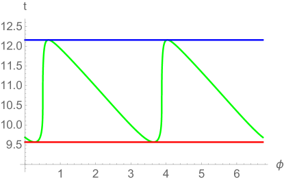
There is a numerical evidence that bound is exact. Moreover, the both bounds and contain just one value of , so they can be used for reliable numerical evaluation of the first conjugate time.
10 Conclusion
In this work we used several methods for bounding conjugate points:
-
•
direct estimate of Jacobian of the exponential mapping via comparison functions (for ),
-
•
homotopy invariance of the index of the second variation (for ),
-
•
projection to lower-dimensional SR minimizers (for ).
We believe that these methods can be useful for bounding conjugate points in other SR problems.
Using the estimate of cut time obtained in work [36] (Theorem 1) and the estimate of conjugate time proved in this work (Theorem 2), one can prove Conjecture 1 and get a description of global structure of the exponential map in the SR problem on the Cartan group. So we can reduce this problem to solving a system of algebraic equations. This will be the subject of forthcoming works.
Appendix A Appendix:
Explicit formulas for coefficients of Jacobian
In this appendix we present explicit formulas for the coefficients , of the Jacobian in the domain .
| (A.1) | |||
| (A.2) | |||
Here and are elliptic integrals of the first and second kinds [42].
References
- [1] A. Agrachev, D. Barilari, U. Boscain, A comprehensive introduction to sub-Riemannian geometry, Cambridge University Press, 2019.
- [2] Agrachev A.A., Geometry of optimal control problems and Hamiltonian systems. In: Nonlinear and Optimal Control Theory, Lecture Notes in Mathematics. CIME, 1932, Springer Verlag, 2008, 1–59.
- [3] A.A. Agrachev and Yu. L. Sachkov, An Intrinsic Approach to the Control of Rolling Bodies, Proceedings of the 38-th IEEE Conference on Decision and Control, vol. 1, Phoenix, Arizona, USA, December 7–10, 1999, 431–435.
- [4] Agrachev A.A., Sachkov Yu.L., Control theory from the geometric viewpoint, Springer, 2004.
- [5] A. A. Agrachev, A. A. Sarychev, Filtration of a Lie algebra of vector fields and nilpotent approximation of control systems, Dokl. Akad. Nauk SSSR, 295 (1987), English transl. in Soviet Math. Dokl., 36 (1988), 104–108.
- [6] A. Anzaldo-Meneses, F. Monroy-Pérez, Charges in magnetic fields and sub-Riemannian geodesics, In: Contemporary trends in nonlinear geometric control theory and its applications, A. Anzaldo-Meneses, B. Bonnard, J.P. Gauthier, F. Monroy-Pérez Eds., World Scientific, 2002, pp. 183–202.
- [7] A.Ardentov, E. Hakavuori, Cut time in the sub-Riemannian problem on the Cartan group, in preparation.
- [8] Ardentov A.A., Sachkov Yu.L., Extremal trajectories in nilpotent sub-Riemannian problem on the Engel group, Matematicheskii Sbornik, 2011, Vol. 202, No. 11, 31–54 (in Russian).
- [9] A.A. Ardentov, Yu. L. Sachkov, Conjugate points in nilpotent sub-Riemannian problem on the Engel group, Journal of Mathematical Sciences, Vol. 195, No. 3, December, 2013, 369–390.
- [10] A.A. Ardentov, Yu. L. Sachkov, Cut time in sub-Riemannian problem on Engel group, ESAIM: Control, Optimisation and Calculus of Variations, 21 (2015), 958–988.
- [11] A.A. Ardentov, Yu. L. Sachkov, Maxwell Strata and Cut Locus in the Sub-Riemannian Problem on the Engel Group, Regular and Chaotic Dynamics, December 2017, Vol. 22, Issue 8, pp 909–936.
- [12] Bellaiche A. The tangent space in sub-Riemannian geometry// In: Sub-Riemannian geometry, A. Bellaiche and J.-J. Risler, Eds., Birkhäuser, Basel, Swizerland, 1996, 1–78.
- [13] V. N. Berestovskii, I. A. Zubareva, Geodesics and shortest arcs of a special sub-Riemannian metric on the Lie group SO(3), Siberian Math. J., 56:4 (2015), 601–611
- [14] V. N. Berestovskiǐ, I. A. Zubareva, Geodesics and shortest arcs of a special sub-Riemannian metric on the Lie group SL(2), Siberian Math. J., 57:3 (2016), 411–424
- [15] Bizyaev I. A., Borisov A. V., Kilin A. A., Mamaev I. S., Integrability and Nonintegrability of Sub-Riemannian Geodesic Flows on Carnot Groups, Regular and Chaotic Dynamics, 2016, vol. 21, no. 6, pp. 759-774
- [16] Boscain U., Rossi F., Invariant Carnot-Caratheodory metrics on , , and Lens Spaces. SIAM, Journal on Control and Optimization, 2008, 47, 1851-1878.
- [17] Brockett R. Control theory and singular Riemannian geometry// In: New Directions in Applied Mathematics, (P. Hilton and G. Young eds.), Springer-Verlag, New York, 11–27.
- [18] Brockett R., Dai L. Non-holonomic kinematics and the role of elliptic functions in constructive controllability// In: Nonholonomic Motion Planning, Z. Li and J. Canny, Eds., Kluwer, Boston, 1993, 1–21.
- [19] Ya. Butt, A.I. Bhatti, Yu. Sachkov, Cut Locus and Optimal Synthesis in Sub-Riemannian Problem on the Lie Group , Journal of Dynamical and Control Systems, 23 (2017), 155–195
- [20] E. Cartan, Lès systemes de Pfaff a cinque variables et lès equations aux derivees partielles du second ordre, Ann. Sci. Ècole Normale 27 (1910), 3: 109–192.
- [21] L.Euler, Methodus inveniendi lineas curvas maximi minimive proprietate gaudentes, sive Solutio problematis isoperimitrici latissimo sensu accepti, Lausanne, Geneva, 1744.
- [22] V.Jurdjevic, The geometry of the plate-ball problem, Arch. Rat. Mech. Anal., v. 124 (1993), 305–328.
- [23] Jurdjevic V. Geometric Control Theory, Cambridge University Press, 1997.
- [24] J.P. Laumond, Nonholonomic motion planning for mobile robots, LAAS Report 98211, May 1998, LAAS-CNRS, Toulouse, France.
- [25] L.Lokutsievskii, Yu. Sachkov, Liouville nonintegrability of sub-Riemannian problems on free Carnot groups of step 4, Sbornik: Mathematics, 209:5 (2018), 74–-119.
- [26] A.E.H.Love, A Treatise on the Mathematical Theory of Elasticity, 4th ed., New York: Dover, 1927.
- [27] A. Marigo and A. Bicchi, Rolling bodies with regular surface: the holonomic case, In Differential geometry and control: Summer Research Institute on Differential Geometry and Control, June 29–July 19, 1997, Univ. Colorado, Boulder, G. Ferreyra et al., eds., Proc. Sympos. Pure Math. 64, Amer. Math. Soc., Providence, RI, 1999, 241–256.
- [28] R. Montgomery, A Tour of Subriemannian Geometries, Their Geodesics and Applications. American Mathematical Society (2002).
- [29] O. Myasnichenko. Nilpotent (3, 6) sub-Riemannian problem, Journal of Dynamical and Control Systems, 8:4 (2002), pp. 573–597
- [30] Pontryagin L.S., Boltayanskii V.G., Gamkrelidze R.V.,Mishchenko E.F., The mathematical theory of optimal processes, Wiley (1962) (Translated from Russian).
- [31] M. M. Postnikov, Lie groups and Lie algebras (in Russian), Nauka, Moscow, 1982.
- [32] Sachkov Yu.L., Exponential map in the generalized Dido problem (in Russian). Mat. Sb., 2003, 194:9, 63–90.
- [33] Sachkov Yu.L., Symmetries of Flat Rank Two Distributions and Sub-Riemannian Structures, Transactions of the American Mathematical Society, 356 (2004), 2: 457–494.
- [34] Sachkov Yu.L., Discrete symmetries in the generalized Dido problem, Sbornik: Mathematics (2006),197(2): 95–116.
- [35] Sachkov Yu.L., The Maxwell set in the generalized Dido problem, Sbornik: Mathematics (2006),197(4): 123–150.
- [36] Sachkov Yu.L., Complete description of the Maxwell strata in the generalized Dido problem, Sbornik: Mathematics (2006),197(6): 111-160.
- [37] Sachkov Yu.L., Conjugate points in Euler’s elastic problem // Journal of Dynamical and Control Systems (Springer, New York), Vol 14 (2008), No. 3, 409–439.
- [38] Sachkov Yu.L., Conjugate and cut time in sub-Riemannian problem on the group of motions of a plane, ESAIM: COCV, 16 (2010), 1018–1039.
- [39] Sarychev A.V., The index of second variation of a control system, Matem. Sbornik 113 (1980), 464–486. English transl. in: Math. USSR Sbornik 41 (1982), 383–401.
- [40] M. Vendittelli, J.P. Laumond, and G. Oriolo, Steering nonholonomic systems via nilpotent approximations: The general two-trailer system, IEEE International Conference on Robotics and Automation, May 10–15, Detroit, MI, 1999.
- [41] A.M. Vershik, V.Y. Gershkovich, Nonholonomic Dynamical Systems. Geometry of distributions and variational problems. (Russian) In: Itogi Nauki i Tekhniki: Sovremennye Problemy Matematiki, Fundamental’nyje Napravleniya, Vol. 16, VINITI, Moscow, 1987, 5–85. (English translation in: Encyclopedia of Math. Sci. 16, Dynamical Systems 7, Springer Verlag.)
- [42] Whittaker E.T., Watson G.N., A Course of Modern Analysis, Cambridge University Press, 1927.