YITP-20-71

IPMU20-0060


Holographic Pseudo Entropy

Yoshifumi Nakataa,b, Tadashi Takayanagia,c,d, Yusuke Takia,

Kotaro Tamaokaa and Zixia Weia

aCenter for Gravitational Physics,
Yukawa Institute for Theoretical Physics, Kyoto University,
Kitashirakawa Oiwakecho, Sakyo-ku, Kyoto 606-8502, Japan

bJST, PRESTO,
4-1-8 Honcho, Kawaguchi, Saitama 332-0012, Japan

cInamori Research Institute for Science,
620 Suiginya-cho, Shimogyo-ku, Kyoto 600-8411 Japan

dKavli Institute for the Physics and Mathematics of the Universe (WPI),
University of Tokyo, Kashiwa, Chiba 277-8582, Japan

We introduce a quantity, called pseudo entropy, as a generalization of entanglement entropy via post-selection. In the AdS/CFT correspondence, this quantity is dual to areas of minimal area surfaces in time-dependent Euclidean spaces which are asymptotically AdS. We study its basic properties and classifications in qubit systems. In specific examples, we provide a quantum information theoretic meaning of this new quantity as an averaged number of Bell pairs when the post-selection is performed. We also present properties of the pseudo entropy for random states. We then calculate the pseudo entropy in the presence of local operator excitations for both the two dimensional free massless scalar CFT and two dimensional holographic CFTs. We find a general property in CFTs that the pseudo entropy is highly reduced when the local operators get closer to the boundary of the subsystem. We also compute the holographic pseudo entropy for a Janus solution, dual to an exactly marginal perturbation of a two dimensional CFT and find its agreement with a perturbative calculation in the dual CFT. We show the linearity property holds for holographic states, where the holographic pseudo entropy coincides with a weak value of the area operator. Finally, we propose a mixed state generalization of pseudo entropy and give its gravity dual.

1 Introduction

In recent developments of theoretical physics, entanglement entropy has played crucial roles, unifying theoretical frameworks in quantum information theory, condensed matter physics, and high energy physics. Entanglement entropy measures the amount of quantum entanglement, which is an important resource in quantum information theory [2, 3]. It also becomes a useful quantum order parameter in condensed matter physics [4, 5]. In high energy physics, this quantity provides a universal characterization of degrees of freedom in quantum field theories [6, 7, 8, 9, 10]. Moreover, the geometric formula of entanglement entropy [11, 12, 13], based on the anti de-Sitter space/ conformal field theory (AdS/CFT) correspondence [14, 15] or holography in a more general context [16, 17], motivates us expect that spacetimes in gravity emerge from quantum entanglement [18, 19].

The AdS/CFT relates path integrals in conformal field theories (CFTs) to gravitational partition functions in anti-de Sitter (AdS) spaces in an equivalent way [14, 15]. This allows us to understand quantum states in quantum many-body systems, which are normally algebraically complicated, in the light of a much simpler geometrical language. One typical example of this advantage of AdS/CFT is the computation of entanglement entropy. In AdS/CFT, the entanglement entropy in CFTs can be computed as the area of extremal surface [11, 12], whose derivations based on the bulk-boundary correspondence were given in [20, 21]. The entanglement entropy is defined by dividing the Hilbert space as =ABtensor-productsubscript𝐴subscript𝐵\mathcal{H}=\mathcal{H}_{A}\otimes\mathcal{H}_{B} and by calculating the von Neumann entropy

S(ρA)=Tr[ρAlogρA],𝑆subscript𝜌𝐴Trdelimited-[]subscript𝜌𝐴subscript𝜌𝐴\displaystyle S(\rho_{A})=-\mbox{Tr}[\rho_{A}\log\rho_{A}], (1.1)

where ρA=TrB[|ΨΨ|]subscript𝜌𝐴subscriptTr𝐵delimited-[]ketΨbraΨ\rho_{A}=\mbox{Tr}_{B}[|\Psi\rangle\langle\Psi|] is the reduced density matrix for the total quantum state |ΨketΨ|\Psi\rangle\in\mathcal{H}. At the AdS boundary, the extremal surface, whose area gives the above entanglement entropy, is supposed to end on the boundary of A𝐴A.

In a static asymptotically AdS spacetime, the extremal surface sits on the canonical time slice and therefore coincides with the minimal area surface on that slice [11]. This static setup can be Wick rotated into a Euclidean AdS/CFT setup in a straightforward way. On the other hand, in a generic asymptotically AdS spacetime which is time-dependent, there is no common canonical time slice on which extremal surfaces at a fixed boundary time extend [12]. The Wick rotation which brings this Lorentzian time-dependent metric into a Euclidean one is subtle as the metric can become complex valued in general under this procedure.

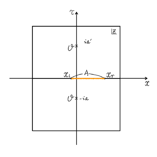
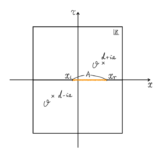
This raises a simple question: what is the meaning of the area of minimal surfaces in Euclidean asymptotically AdS spaces which are time-dependent? Via the AdS/CFT, such a geometry is typically dual to a path-integral in the dual CFT with time-dependent sources as sketched in figure 1. We write the coordinate of the Euclidean time as τ𝜏\tau. By focusing on a particular Euclidean time τ=0𝜏0\tau=0, the upper path-integral (i.e. 0τ<0𝜏0\leq\tau<\infty) defines a quantum state |φket𝜑|{\varphi}\rangle, while the lower one (i.e. <τ0)-\infty<\tau\leq 0) defines another quantum state |ψket𝜓|\psi\rangle. In particular, the gravity partition function on the whole Euclidean space, which is asymptotically AdS, coincides with the inner product φ|ψinner-product𝜑𝜓\langle{\varphi}|\psi\rangle.

Refer to caption
Figure 1: The calculation of holographic pseudo entropy. At the time specified as the dotted circle, the bra state and ket state are different. Accordingly, the asymptotically AdS Euclidean geometry is time-dependent. The dots are excitations by inserting external sources or operators to CFTs.

In this paper we argue that the area of a minimal area surface in a (generically time-dependent) Euclidean asymptotically AdS space calculates the following CFT quantity analogous to the von Neumann entropy, which we call pseudo entropy:

S(𝒯Aψ|φ)=Tr[𝒯Aψ|φlog𝒯Aψ|φ],𝑆subscriptsuperscript𝒯conditional𝜓𝜑𝐴Trdelimited-[]subscriptsuperscript𝒯conditional𝜓𝜑𝐴subscriptsuperscript𝒯conditional𝜓𝜑𝐴\displaystyle S(\mathcal{T}^{\psi|{\varphi}}_{A})=-\mbox{Tr}[\mathcal{T}^{\psi|{\varphi}}_{A}\log\mathcal{T}^{\psi|{\varphi}}_{A}], (1.2)

where 𝒯Aψ|φ=TrB[𝒯ψ|φ]subscriptsuperscript𝒯conditional𝜓𝜑𝐴subscriptTr𝐵delimited-[]superscript𝒯conditional𝜓𝜑\mathcal{T}^{\psi|{\varphi}}_{A}=\mbox{Tr}_{B}[\mathcal{T}^{\psi|{\varphi}}] is defined from the transition matrix:

𝒯ψ|φ|ψφ|φ|ψ.superscript𝒯conditional𝜓𝜑ket𝜓bra𝜑inner-product𝜑𝜓\mathcal{T}^{\psi|{\varphi}}\equiv\frac{|{\psi}\rangle\langle{{\varphi}}|}{\braket{{\varphi}}{\psi}}. (1.3)

We call 𝒯Aψ|φsubscriptsuperscript𝒯conditional𝜓𝜑𝐴\mathcal{T}^{\psi|{\varphi}}_{A} a reduced transition matrix. Notice that these matrices 𝒯Aψ|φsubscriptsuperscript𝒯conditional𝜓𝜑𝐴\mathcal{T}^{\psi|{\varphi}}_{A} and 𝒯ψ|φsuperscript𝒯conditional𝜓𝜑\mathcal{T}^{\psi|{\varphi}} are not Hermitian in general and therefore we cannot regard them as quantum (mixed) states in an ordinary sense. Indeed, in general the entropic quantity S(𝒯Aψ|φ)𝑆subscriptsuperscript𝒯conditional𝜓𝜑𝐴S(\mathcal{T}^{\psi|{\varphi}}_{A}) is complex valued. Nevertheless, such generalized density matrices naturally arise in the context of the post-selection where the initial state |ψket𝜓|\psi\rangle is post-selected into the state |φket𝜑|{\varphi}\rangle. In the post-selection setup, a quantity analogue to the expectation value of an observable operator 𝒪𝒪{\cal O} can be defined by

𝒪=φ|𝒪|ψφ|ψ=Tr[𝒪𝒯ψ|φ].delimited-⟨⟩𝒪quantum-operator-product𝜑𝒪𝜓inner-product𝜑𝜓Trdelimited-[]𝒪superscript𝒯conditional𝜓𝜑\displaystyle\langle{\cal O}\rangle=\frac{\langle{\varphi}|{\cal O}|\psi\rangle}{\langle{\varphi}|\psi\rangle}=\mbox{Tr}[{\cal O}\mathcal{T}^{\psi|{\varphi}}]. (1.4)

This is known as a weak value [22] and has been studied since it can be used in certain experiments (refer e.g. [23] for a review). Note that this quantity also takes complex values in general. Refer to [24] for studies of conditional entropy of post-selected states.

The main purpose of this paper is to introduce the novel quantity (1.2), which we call pseudo entropy, in quantum many-body systems and field theories mainly motivated by the above holographic consideration.111We should distinguish the pseudo entropy, defined through the post-selection process as we explained in the above, from the (standard) entanglement entropy after projection measurements. The latter was studied in [25, 26] for two dimensional CFTs. Since this quantity provides a new fundamental relationship between geometries in gravity and quantum information in CFT, we expect that this helps us to understand the basic principle of the AdS/CFT correspondence and eventually quantum gravity. Also, its involving the information of two independent quantum states makes it largely different from known quantum informational quantities which are related to geometries in gravity. At the same time, this quantity can serve as a new class of order parameters in quantum many-body systems.

This paper is organized as follows. In section 2, we will present the basic definitions and properties of pseudo entropy. We will also give a general replica method which will be used to calculate the pseudo entropy in quantum field theories. Moreover, we will explain the holographic calculation of pseudo entropy in AdS/CFT. In section 3, we examine properties of pseudo entropy in qubit systems. Firstly we classify the reduced transition matrices and also point out a monotonicity property in two qubit systems. Next we will provide an interpretation of pseudo entropy for a class of transition matrices in terms of averaged number of Bell pairs that could have been distilled from the intermediate state when a final state is post-selected. We also show a couple of typical properties of pseudo entropy. In section 4, we will present computations of pseudo Rényi entropy in a two dimensional free scalar CFT by choosing the quantum states to be locally excited states. In section 5, we study holographic pseudo entropy. After we explain its general properties, we give explicit results in a Janus AdS/CFT, which corresponds to the pseudo entropy for CFT states with two different external fields. We also present results of holographic pseudo entropy for locally excited states. We will also show the linearity is satisfied in our holographic formula. In section 6, we give a mixed state generalization of pseudo entropy, based on reflected entropy. In section 7, we summarize our conclusions and discuss future problems. In appendix A, we give a detailed discussion of the expressions of pseudo (Rényi) entropy. In appendix B, we present a calculation of pseudo entropy for thermo field double states. In appendix C, we calculate pseudo entropy for two coupled harmonic oscillators. In appendix D, we provide how to compute the average of the pseudo entropy for random states. In appendix E, we analyze pseudo entropy for quantum states with perturbative external fields. In appendix F, we study the pseudo entropy and fidelity for local operator excited states. In appendix G, we leave a proof for the linearity of pseudo entropy associated with linear combination of heavy states.

2 Basics of Pseudo Entropy

Here we introduce a quantity, called pseudo entropy, which is a generalization of entropy from an ordinary quantum state to a process of a post-selection. After we give its definition and basic properties, we explain general methods to calculate this quantity in quantum field theories and the AdS/CFT.

2.1 Definition of Pseudo Entropy

Consider two pure quantum states |ψket𝜓|\psi\rangle and |φket𝜑|{\varphi}\rangle which satisfy φ|ψ0inner-product𝜑𝜓0\braket{{\varphi}}{\psi}\neq 0. We introduce the transition matrix between them 𝒯ψ|φsuperscript𝒯conditional𝜓𝜑\mathcal{T}^{\psi|{\varphi}} as follows:

𝒯ψ|φ|ψφ|φ|ψ,superscript𝒯conditional𝜓𝜑ket𝜓bra𝜑inner-product𝜑𝜓\mathcal{T}^{\psi|{\varphi}}\equiv\frac{|{\psi}\rangle\langle{{\varphi}}|}{\braket{{\varphi}}{\psi}}, (2.1)

which is normalized such that its trace is one.

Note that this satisfies

(𝒯ψ|φ)n=𝒯ψ|φ,superscriptsuperscript𝒯conditional𝜓𝜑𝑛superscript𝒯conditional𝜓𝜑\displaystyle\left(\mathcal{T}^{\psi|{\varphi}}\right)^{n}=\mathcal{T}^{\psi|{\varphi}}, (2.2)

and thus we find

Tr[(𝒯ψ|φ)n]=1,Trdelimited-[]superscriptsuperscript𝒯conditional𝜓𝜑𝑛1\displaystyle\mbox{Tr}[\left(\mathcal{T}^{\psi|{\varphi}}\right)^{n}]=1, (2.3)

for any n+𝑛superscriptn\in\mathbb{N}^{+}. Under the exchange of |ψket𝜓|\psi\rangle and |φket𝜑|{\varphi}\rangle, we find

𝒯ψ|φ=[𝒯φ|ψ].superscript𝒯conditional𝜓𝜑superscriptdelimited-[]superscript𝒯conditional𝜑𝜓\displaystyle\mathcal{T}^{\psi|{\varphi}}=\left[\mathcal{T}^{{\varphi}|\psi}\right]^{\dagger}. (2.4)

We divide the total system into two subsystems A𝐴A and B𝐵B such that the total Hilbert space \mathcal{H} is given by a tensor product:

=AB.tensor-productsubscript𝐴subscript𝐵\displaystyle\mathcal{H}=\mathcal{H}_{A}\otimes\mathcal{H}_{B}. (2.5)

Accordingly we introduce the reduced transition matrix

𝒯Aψ|φTrB[𝒯ψ|φ]=TrB[|ψφ|φ|ψ].subscriptsuperscript𝒯conditional𝜓𝜑𝐴subscriptTr𝐵delimited-[]superscript𝒯conditional𝜓𝜑subscriptTr𝐵delimited-[]ket𝜓bra𝜑inner-product𝜑𝜓\mathcal{T}^{\psi|{\varphi}}_{A}\equiv\mathrm{Tr}_{B}\left[{\mathcal{T}}^{\psi|{\varphi}}\right]=\mbox{Tr}_{B}\left[\frac{|\psi\rangle\langle{{\varphi}}|}{\braket{{\varphi}}{\psi}}\right]. (2.6)

Now we introduce “n𝑛n-th Rényi entropy” of the transition matrix 𝒯Aψ|φsubscriptsuperscript𝒯conditional𝜓𝜑𝐴\mathcal{T}^{\psi|{\varphi}}_{A} in the same way as we define the n𝑛n-th Rényi entropy of a quantum state ρ𝜌\rho:

S(n)(𝒯Aψ|φ)11nlogTr[(𝒯Aψ|φ)n](n+,n2),superscript𝑆𝑛subscriptsuperscript𝒯conditional𝜓𝜑𝐴11𝑛Trdelimited-[]superscriptsubscriptsuperscript𝒯conditional𝜓𝜑𝐴𝑛formulae-sequence𝑛superscript𝑛2\displaystyle S^{(n)}(\mathcal{T}^{\psi|{\varphi}}_{A})\equiv\frac{1}{1-n}\log\mbox{Tr}\left[(\mathcal{T}^{\psi|{\varphi}}_{A})^{n}\right]\leavevmode\nobreak\ \leavevmode\nobreak\ (n\in\mathbb{N}^{+},n\geq 2), (2.7)

where we can simply choose the branch of the log function: π<Im[log(z)]π𝜋Imdelimited-[]𝑧𝜋-\pi<{\rm Im}\left[\log(z)\right]\leq\pi. We call this quantity S(n)(𝒯Aψ|φ)superscript𝑆𝑛subscriptsuperscript𝒯conditional𝜓𝜑𝐴S^{(n)}({\mathcal{T}}^{\psi|{\varphi}}_{A}) the pseudo n𝑛n-th Rényi entropy. In the following of this paper, we use log(z)𝑧\log(z) to denote the principal value of the logarithmic function. Notice that, since 𝒯Aψ|φsubscriptsuperscript𝒯conditional𝜓𝜑𝐴\mathcal{T}^{\psi|{\varphi}}_{A} is not a quantum state (i.e. Hermitian and non-negative), this pseudo Rényi entropy takes a complex value in general. Note also that when B𝐵B is empty, i.e. 𝒯Aψ|φ=𝒯ψ|φsubscriptsuperscript𝒯conditional𝜓𝜑𝐴superscript𝒯conditional𝜓𝜑\mathcal{T}^{\psi|{\varphi}}_{A}=\mathcal{T}^{\psi|{\varphi}}, it is obvious that its entropy is vanishing

S(n)(𝒯ψ|φ)=0.superscript𝑆𝑛superscript𝒯conditional𝜓𝜑0\displaystyle S^{(n)}(\mathcal{T}^{\psi|{\varphi}})=0. (2.8)

This can be easily seen from (2.3).

For n+𝑛superscriptn\in\mathbb{N}^{+}, n2𝑛2n\geq 2, S(n)(𝒯Aψ|φ)superscript𝑆𝑛subscriptsuperscript𝒯conditional𝜓𝜑𝐴S^{(n)}({\mathcal{T}}^{\psi|{\varphi}}_{A}) admits an alternative expression

S(n)(𝒯Aψ|φ)=11nlog[jλj(𝒯Aψ|φ)n],superscript𝑆𝑛subscriptsuperscript𝒯conditional𝜓𝜑𝐴11𝑛subscript𝑗subscript𝜆𝑗superscriptsubscriptsuperscript𝒯conditional𝜓𝜑𝐴𝑛\displaystyle S^{(n)}({\mathcal{T}}^{\psi|{\varphi}}_{A})=\frac{1}{1-n}\log\left[\sum_{j}\lambda_{j}({\mathcal{T}}^{\psi|{\varphi}}_{A})^{n}\right], (2.9)

where λj(𝒯Aψ|φ)subscript𝜆𝑗subscriptsuperscript𝒯conditional𝜓𝜑𝐴\lambda_{j}({\mathcal{T}}^{\psi|{\varphi}}_{A}) are the eigenvalues of 𝒯Aψ|φsubscriptsuperscript𝒯conditional𝜓𝜑𝐴{\mathcal{T}}^{\psi|{\varphi}}_{A}.222 Note that since 𝒯Aψ|φsubscriptsuperscript𝒯conditional𝜓𝜑𝐴{\mathcal{T}}^{\psi|{\varphi}}_{A} is not Hermitian in general, we cannot always diagonalize it either by the unitary matrices or even by regular matrices. Nevertheless, its eigenvalues are always well-defined and (2.9) follows directly from a Jordan decomposition of 𝒯Aψ|φsubscriptsuperscript𝒯conditional𝜓𝜑𝐴{\mathcal{T}}^{\psi|{\varphi}}_{A}. Refer to appendix A for a review of Jordan normal form and an argument about pseudo Rényi entropy using it.

This expression can be extended to n+\{1}𝑛\superscript1n\in\mathbb{R}^{+}\backslash\{1\} where ansuperscript𝑎𝑛a^{n} is defined as

anenlog(a)(a,n+).superscript𝑎𝑛superscript𝑒𝑛𝑎formulae-sequence𝑎𝑛superscript\displaystyle a^{n}\equiv e^{n\log(a)}\leavevmode\nobreak\ \leavevmode\nobreak\ (a\in\mathbb{C},n\in\mathbb{R}^{+}). (2.10)

This allows us to take the n1𝑛1n\rightarrow 1 limit and define a von Neumann version of pseudo entropy as

S(𝒯Aψ|φ)limn1S(n)(𝒯Aψ|φ)=jλj(𝒯Aψ|φ)log[λj(𝒯Aψ|φ)].𝑆subscriptsuperscript𝒯conditional𝜓𝜑𝐴subscript𝑛1superscript𝑆𝑛subscriptsuperscript𝒯conditional𝜓𝜑𝐴subscript𝑗subscript𝜆𝑗subscriptsuperscript𝒯conditional𝜓𝜑𝐴subscript𝜆𝑗subscriptsuperscript𝒯conditional𝜓𝜑𝐴\displaystyle S({\mathcal{T}}^{\psi|{\varphi}}_{A})\equiv\lim_{n\rightarrow 1}S^{(n)}({\mathcal{T}}^{\psi|{\varphi}}_{A})=-\sum_{j}\lambda_{j}({\mathcal{T}}^{\psi|{\varphi}}_{A})\log\left[\lambda_{j}({\mathcal{T}}^{\psi|{\varphi}}_{A})\right]. (2.11)

We call this the pseudo entropy of 𝒯Aψ|φsubscriptsuperscript𝒯conditional𝜓𝜑𝐴{\mathcal{T}}^{\psi|{\varphi}}_{A}, or the entanglement pseudo entropy of A𝐴A.

Finally, we would like to note that pseudo (Rényi) entropy can be expressed in matrix form as follows:

S(n)(𝒯Aψ|φ)=11nlogTr(𝒯Aψ|φ)n,(n+\{1})superscript𝑆𝑛subscriptsuperscript𝒯conditional𝜓𝜑𝐴11𝑛Trsuperscriptsubscriptsuperscript𝒯conditional𝜓𝜑𝐴𝑛𝑛\superscript1\displaystyle S^{(n)}({\mathcal{T}}^{\psi|{\varphi}}_{A})=\frac{1}{1-n}\log\mathrm{Tr}\left({\mathcal{T}}^{\psi|{\varphi}}_{A}\right)^{n},\leavevmode\nobreak\ \leavevmode\nobreak\ (n\in\mathbb{R}^{+}\backslash\{1\}) (2.12)
S(𝒯Aψ|φ)=Tr(𝒯Aψ|φlog𝒯Aψ|φ),𝑆subscriptsuperscript𝒯conditional𝜓𝜑𝐴Trsubscriptsuperscript𝒯conditional𝜓𝜑𝐴subscriptsuperscript𝒯conditional𝜓𝜑𝐴\displaystyle S({\mathcal{T}}^{\psi|{\varphi}}_{A})=-\mathrm{Tr}\left({\mathcal{T}}^{\psi|{\varphi}}_{A}\log{\mathcal{T}}^{\psi|{\varphi}}_{A}\right), (2.13)

if we give proper treatments to some subtle points. See appendix A for a discussion on it.

A few comments are in order. In the main parts of this paper, especially in the context of quantum field theories and the AdS/CFT correspondence, we focus on the case where Tr[(𝒯Aψ|φ)n]Trdelimited-[]superscriptsubscriptsuperscript𝒯conditional𝜓𝜑𝐴𝑛\mbox{Tr}\left[(\mathcal{T}^{\psi|{\varphi}}_{A})^{n}\right] is positive. Therefore, we do not need to worry about the choice of branch of the log function. In more generic examples, Tr[(𝒯Aψ|φ)n]Trdelimited-[]superscriptsubscriptsuperscript𝒯conditional𝜓𝜑𝐴𝑛\mbox{Tr}\left[(\mathcal{T}^{\psi|{\varphi}}_{A})^{n}\right] takes complex values and the choice of the branch is important. Though in the above we just chose a simple one π<Im[log(z)]π𝜋Imdelimited-[]𝑧𝜋-\pi<{\rm Im}\left[\log(z)\right]\leq\pi,333We would like to thank very much a referee for pointing out that this particular choice of the branch may be relevant when one wants to apply Carlson’s theorem to prove the uniqueness of extension of holographic pseudo Rényi entropy to non-integer replica number n𝑛n, under the assumption that all the eigenvalues of the corresponding reduced transition matrix are not negative numbers. We would like to leave the precise discussion and justifications for the assumptions above as a future problem. we would like to keep open the possibility that there might be a better choice for applications in physics, leaving as a future problem.

2.2 Basic Properties of Pseudo Entropy

First we have to note that the pseudo entropy S(n)(𝒯Aψ|φ)superscript𝑆𝑛subscriptsuperscript𝒯conditional𝜓𝜑𝐴S^{(n)}({\mathcal{T}}^{\psi|{\varphi}}_{A}) is complex valued in general because the eigenvalues of the transition matrix 𝒯Aψ|φsubscriptsuperscript𝒯conditional𝜓𝜑𝐴\mathcal{T}^{\psi|{\varphi}}_{A} can be complex. Only in special choices of states |ψket𝜓|\psi\rangle and |φket𝜑|{\varphi}\rangle, we find real and non-negative eigenvalues of 𝒯Aψ|φsubscriptsuperscript𝒯conditional𝜓𝜑𝐴\mathcal{T}^{\psi|{\varphi}}_{A}, which we will be especially interested in this paper.

In general, we can easily prove the following basic properties for n+𝑛superscriptn\in\mathbb{R}^{+},

(i)If|ψhas no entanglement, then S(n)(𝒯Aψ|φ)=0.𝑖Ifket𝜓has no entanglement, then superscript𝑆𝑛subscriptsuperscript𝒯conditional𝜓𝜑𝐴0\displaystyle(i)\ \mbox{If}\ |\psi\rangle\ \mbox{has no entanglement, then }\ S^{(n)}(\mathcal{T}^{\psi|{\varphi}}_{A})=0. (2.14)
(ii)If Tr(𝒯Aψ|φ)n and all eigenvalues of 𝒯Aψ|φ are in \,𝑖𝑖If Tr(𝒯Aψ|φ)n and all eigenvalues of 𝒯Aψ|φ are in \,\displaystyle(ii)\ \mbox{If $\mathrm{Tr}({\mathcal{T}}^{\psi|{\varphi}}_{A})^{n}$ and all eigenvalues of ${\mathcal{T}}^{\psi|{\varphi}}_{A}$ are in $\mathbb{C}\backslash\mathbb{R}^{-}$, }
then S(n)(𝒯Aψ|φ)=S(n)(𝒯Aφ|ψ).then superscript𝑆𝑛subscriptsuperscript𝒯conditional𝜓𝜑𝐴superscript𝑆𝑛superscriptsubscriptsuperscript𝒯conditional𝜑𝜓𝐴\displaystyle\leavevmode\nobreak\ \leavevmode\nobreak\ \leavevmode\nobreak\ \leavevmode\nobreak\ \leavevmode\nobreak\ \mbox{then }S^{(n)}(\mathcal{T}^{\psi|{\varphi}}_{A})=S^{(n)}(\mathcal{T}^{{\varphi}|\psi}_{A})^{*}. (2.15)
(iii)S(n)(𝒯Aψ|φ)=S(n)(𝒯Bψ|φ).𝑖𝑖𝑖superscript𝑆𝑛subscriptsuperscript𝒯conditional𝜓𝜑𝐴superscript𝑆𝑛subscriptsuperscript𝒯conditional𝜓𝜑𝐵\displaystyle(iii)\ S^{(n)}(\mathcal{T}^{\psi|{\varphi}}_{A})=S^{(n)}(\mathcal{T}^{\psi|{\varphi}}_{B}). (2.16)

The property (i)𝑖(i) follows because when |ψ=|ψA|ψ′′Bket𝜓subscriptketsuperscript𝜓𝐴subscriptketsuperscript𝜓′′𝐵|\psi\rangle=|\psi^{\prime}\rangle_{A}|\psi^{\prime\prime}\rangle_{B}, we can show (𝒯Aψ|φ)n=𝒯Aψ|φsuperscriptsubscriptsuperscript𝒯conditional𝜓𝜑𝐴𝑛subscriptsuperscript𝒯conditional𝜓𝜑𝐴\left(\mathcal{T}^{\psi|{\varphi}}_{A}\right)^{n}=\mathcal{T}^{\psi|{\varphi}}_{A}. The property (ii)𝑖𝑖(ii)444The preconditions of (ii)𝑖𝑖(ii) are imposed since log(z)=(log(z))𝑧superscriptsuperscript𝑧\log(z)=\left(\log(z^{*})\right)^{*} does not hold for z𝑧superscriptz\in\mathbb{R}^{-} in our convention. Note that these preconditions are sufficient but not necessary. The precondition “eigenvalues of 𝒯Aψ|φsubscriptsuperscript𝒯conditional𝜓𝜑𝐴{\mathcal{T}}^{\psi|{\varphi}}_{A} are in \\superscript\mathbb{C}\backslash\mathbb{R}^{-}” can be removed if we restrict to n+\{1}𝑛\superscript1n\in\mathbb{N}^{+}\backslash\{1\}. In section 3.5, we will use pseudo Tsallis entropy Tq(𝒯Aψ|φ)=(1tr(𝒯Aψ|φ)q)/(q1)subscript𝑇𝑞subscriptsuperscript𝒯conditional𝜓𝜑𝐴1trsuperscriptsubscriptsuperscript𝒯conditional𝜓𝜑𝐴𝑞𝑞1T_{q}({\mathcal{T}}^{\psi|{\varphi}}_{A})=(1-\mathrm{tr}({\mathcal{T}}^{\psi|{\varphi}}_{A})^{q})/(q-1) for analysis. It satisfies Tq(𝒯Aψ|φ)=Tq(𝒯Aφ|ψ)subscript𝑇𝑞subscriptsuperscript𝒯conditional𝜓𝜑𝐴subscript𝑇𝑞superscriptsubscriptsuperscript𝒯conditional𝜑𝜓𝐴T_{q}({\mathcal{T}}^{\psi|{\varphi}}_{A})=T_{q}({\mathcal{T}}^{{\varphi}|\psi}_{A})^{*} for q+\{1}𝑞\superscript1q\in\mathbb{N}^{+}\backslash\{1\}. can be found from the relation (2.4). The property (iii)𝑖𝑖𝑖(iii) can also be proved via an explicit calculation.

2.3 Classifications of Transition Matrices

In this paper, we mainly focus on the transition matrices which give positive S(n)(𝒯Aψ|φ)superscript𝑆𝑛subscriptsuperscript𝒯conditional𝜓𝜑𝐴S^{(n)}({\mathcal{T}}^{\psi|{\varphi}}_{A}) for n>0𝑛0n>0. To understand how special this class is, we would like to classify the transition matrices.

We start with a Hilbert space {\mathcal{H}} factorized into two parts as =ABtensor-productsubscript𝐴subscript𝐵{\mathcal{H}}={\mathcal{H}}_{A}\otimes{\mathcal{H}}_{B}. Let us denote the set of transition matrices on {\mathcal{H}} as 𝒯()𝒯\mathscr{T}({\mathcal{H}}). Consider several special classes of transition matrices given as follows.

  • 𝒜𝒜\mathscr{A}: The set of transition matrices which give real-valued Tr(𝒯Aψ|φ)nTrsuperscriptsubscriptsuperscript𝒯conditional𝜓𝜑𝐴𝑛\mathrm{Tr}\left({\mathcal{T}}^{\psi|{\varphi}}_{A}\right)^{n} for n>0𝑛0n>0.

  • \mathscr{B}: The set of transition matrices which give nonnegative real S(n)(𝒯Aψ|φ)superscript𝑆𝑛subscriptsuperscript𝒯conditional𝜓𝜑𝐴S^{(n)}({\mathcal{T}}^{\psi|{\varphi}}_{A}) for n>0𝑛0n>0.

  • 𝒞𝒞\mathscr{C}: The set of transition matrices which give 𝒯Aψ|φsubscriptsuperscript𝒯conditional𝜓𝜑𝐴{\mathcal{T}}^{\psi|{\varphi}}_{A} whose eigenvalues are real and nonnegative.

  • 𝒟𝒟\mathscr{D}: The set of transition matrices which give positive semi-definite Hermitian 𝒯Aψ|φsubscriptsuperscript𝒯conditional𝜓𝜑𝐴{\mathcal{T}}^{\psi|{\varphi}}_{A}.

  • \mathscr{E}: The set of transition matrices which give positive semi-definite Hermitian 𝒯Aψ|φsubscriptsuperscript𝒯conditional𝜓𝜑𝐴{\mathcal{T}}^{\psi|{\varphi}}_{A} and positive semi-definite Hermitian 𝒯Bψ|φsubscriptsuperscript𝒯conditional𝜓𝜑𝐵{\mathcal{T}}^{\psi|{\varphi}}_{B}.

It is not difficult to figure out that 𝒟𝒞𝒜𝒯()𝒟𝒞𝒜𝒯\mathscr{E}\subseteq\mathscr{D}\subseteq\mathscr{C}\subseteq\mathscr{B}\subseteq\mathscr{A}\subseteq\mathscr{T}({\mathcal{H}}).

For example, in a trivial setup where dim=dimA=dimB=1dimdimsubscript𝐴dimsubscript𝐵1{\rm dim}{\mathcal{H}}={\rm dim}{\mathcal{H}}_{A}={\rm dim}{\mathcal{H}}_{B}=1 and 𝒯ψ|φ=1superscript𝒯conditional𝜓𝜑1{\mathcal{T}}^{\psi|{\varphi}}=1, these classes degenerate, i.e. =𝒟=𝒞==𝒜=𝒯()𝒟𝒞𝒜𝒯\mathscr{E}=\mathscr{D}=\mathscr{C}=\mathscr{B}=\mathscr{A}=\mathscr{T}({\mathcal{H}}).

In particular, for 2-qubit systems, we find 𝒟𝒞=𝒜𝒯()𝒟𝒞𝒜𝒯\mathscr{E}\subset\mathscr{D}\subset\mathscr{C}=\mathscr{B}\subset\mathscr{A}\subset\mathscr{T}({\mathcal{H}}), as we will see in section 3.1. We will explore various properties of pseudo entropy in qubit systems in section 3.

With these in mind, the only nontrivial part remained in the general inclusion relation 𝒟𝒞𝒜𝒯()𝒟𝒞𝒜𝒯\mathscr{E}\subseteq\mathscr{D}\subseteq\mathscr{C}\subseteq\mathscr{B}\subseteq\mathscr{A}\subseteq\mathscr{T}({\mathcal{H}}) is whether there is a system in which there exists a 𝒯ψ|φsuperscript𝒯conditional𝜓𝜑{\mathcal{T}}^{\psi|{\varphi}} belonging to \mathscr{B} but not to 𝒞𝒞\mathscr{C}. The answer is yes. The following two states in a 2-qutrit system give such an example

|ψ=(UI)|φ,ket𝜓tensor-product𝑈𝐼ket𝜑\displaystyle\ket{\psi}=\left(U\otimes I\right)\ket{{\varphi}}, (2.17)
|φ=25|0|0+110|1|1+110|2|2,ket𝜑tensor-product25ket0ket0tensor-product110ket1ket1tensor-product110ket2ket2\displaystyle\ket{{\varphi}}=\frac{2}{\sqrt{5}}\ket{0}\otimes\ket{0}+\frac{1}{\sqrt{10}}\ket{1}\otimes\ket{1}+\frac{1}{\sqrt{10}}\ket{2}\otimes\ket{2}, (2.18)

where

U=|00|+cosπ4|11|sinπ4|12|+sinπ4|21|+cosπ4|22|.𝑈ket0quantum-operator-product0𝜋41quantum-operator-product1𝜋41quantum-operator-product2𝜋42quantum-operator-product1𝜋42bra2\displaystyle U=|0\rangle\langle 0|+\cos\frac{\pi}{4}|1\rangle\langle 1|-\sin\frac{\pi}{4}|1\rangle\langle 2|+\sin\frac{\pi}{4}|2\rangle\langle 1|+\cos\frac{\pi}{4}|2\rangle\langle 2|. (2.19)

In this case

𝒯Aψ|φsubscriptsuperscript𝒯conditional𝜓𝜑𝐴\displaystyle{\mathcal{T}}^{\psi|{\varphi}}_{A} =5242+1(45|00|+1102|11|1102|12|+1102|21|+1102|22|),absent5242145ket0quantum-operator-product011021quantum-operator-product111021quantum-operator-product211022quantum-operator-product111022bra2\displaystyle=\frac{5\sqrt{2}}{4\sqrt{2}+1}\left(\frac{4}{5}|0\rangle\langle 0|+\frac{1}{10\sqrt{2}}|1\rangle\langle 1|-\frac{1}{10\sqrt{2}}|1\rangle\langle 2|+\frac{1}{10\sqrt{2}}|2\rangle\langle 1|+\frac{1}{10\sqrt{2}}|2\rangle\langle 2|\right),

and the three eigenvalues of 𝒯Aψ|φsubscriptsuperscript𝒯conditional𝜓𝜑𝐴{\mathcal{T}}^{\psi|{\varphi}}_{A} are

88+2p,1+i2(8+2)qeiω,1i2(8+2)qeiω.formulae-sequence882𝑝formulae-sequence1𝑖282𝑞superscript𝑒𝑖𝜔1𝑖282𝑞superscript𝑒𝑖𝜔\displaystyle\frac{8}{8+\sqrt{2}}\equiv p,\leavevmode\nobreak\ \leavevmode\nobreak\ \frac{1+i}{\sqrt{2}(8+\sqrt{2})}\equiv qe^{i\omega},\leavevmode\nobreak\ \leavevmode\nobreak\ \frac{1-i}{\sqrt{2}(8+\sqrt{2})}\equiv qe^{-i\omega}. (2.21)

Clearly this example is in class 𝒜𝒜\mathscr{A} but not in class 𝒞𝒞\mathscr{C}. We can see that, for n<1𝑛1n<1,

Tr(𝒯Aψ|φ)n=pn+(qeiω)n+(qeiω)n=pn+2qncos(nω)>p+2qcosω=1,Trsuperscriptsubscriptsuperscript𝒯conditional𝜓𝜑𝐴𝑛superscript𝑝𝑛superscript𝑞superscript𝑒𝑖𝜔𝑛superscript𝑞superscript𝑒𝑖𝜔𝑛superscript𝑝𝑛2superscript𝑞𝑛𝑛𝜔𝑝2𝑞𝜔1\displaystyle\mathrm{Tr}\left({\mathcal{T}}^{\psi|{\varphi}}_{A}\right)^{n}=p^{n}+(qe^{i\omega})^{n}+(qe^{-i\omega})^{n}=p^{n}+2q^{n}\cos(n\omega)>p+2q\cos\omega=1, (2.22)

and hence S(n)(𝒯Aψ|φ)>0superscript𝑆𝑛subscriptsuperscript𝒯conditional𝜓𝜑𝐴0S^{(n)}({\mathcal{T}}^{\psi|{\varphi}}_{A})>0. For n>1𝑛1n>1,

Tr(𝒯Aψ|φ)n=pn+(qeiω)n+(qeiω)n>pn2qn>0.Trsuperscriptsubscriptsuperscript𝒯conditional𝜓𝜑𝐴𝑛superscript𝑝𝑛superscript𝑞superscript𝑒𝑖𝜔𝑛superscript𝑞superscript𝑒𝑖𝜔𝑛superscript𝑝𝑛2superscript𝑞𝑛0\displaystyle\mathrm{Tr}\left({\mathcal{T}}^{\psi|{\varphi}}_{A}\right)^{n}=p^{n}+(qe^{i\omega})^{n}+(qe^{-i\omega})^{n}>p^{n}-2q^{n}>0. (2.23)

Moreover, for 1<n21𝑛21<n\leq 2,

Tr(𝒯Aψ|φ)n=pn+(qeiω)n+(qeiω)n=pn+2qncos(nω)<p+2qcosω=1,Trsuperscriptsubscriptsuperscript𝒯conditional𝜓𝜑𝐴𝑛superscript𝑝𝑛superscript𝑞superscript𝑒𝑖𝜔𝑛superscript𝑞superscript𝑒𝑖𝜔𝑛superscript𝑝𝑛2superscript𝑞𝑛𝑛𝜔𝑝2𝑞𝜔1\displaystyle\mathrm{Tr}\left({\mathcal{T}}^{\psi|{\varphi}}_{A}\right)^{n}=p^{n}+(qe^{i\omega})^{n}+(qe^{-i\omega})^{n}=p^{n}+2q^{n}\cos(n\omega)<p+2q\cos\omega=1, (2.24)

and for 2<n2𝑛2<n,

Tr(𝒯Aψ|φ)n=pn+(qeiω)n+(qeiω)npn+2qn<p2+2q2=3333+2<1.Trsuperscriptsubscriptsuperscript𝒯conditional𝜓𝜑𝐴𝑛superscript𝑝𝑛superscript𝑞superscript𝑒𝑖𝜔𝑛superscript𝑞superscript𝑒𝑖𝜔𝑛superscript𝑝𝑛2superscript𝑞𝑛superscript𝑝22superscript𝑞2333321\displaystyle\mathrm{Tr}\left({\mathcal{T}}^{\psi|{\varphi}}_{A}\right)^{n}=p^{n}+(qe^{i\omega})^{n}+(qe^{-i\omega})^{n}\leq p^{n}+2q^{n}<p^{2}+2q^{2}=\frac{33}{33+\sqrt{2}}<1. (2.25)

Therefore, 0<Tr(𝒯Aψ|φ)n<10Trsuperscriptsubscriptsuperscript𝒯conditional𝜓𝜑𝐴𝑛10<\mathrm{Tr}\left({\mathcal{T}}^{\psi|{\varphi}}_{A}\right)^{n}<1 for n>1𝑛1n>1 and hence S(n)(𝒯Aψ|φ)>0superscript𝑆𝑛subscriptsuperscript𝒯conditional𝜓𝜑𝐴0S^{(n)}({\mathcal{T}}^{\psi|{\varphi}}_{A})>0. On the other hand, we can explicitly confirm that S(𝒯Aψ|φ)>0𝑆subscriptsuperscript𝒯conditional𝜓𝜑𝐴0S({\mathcal{T}}^{\psi|{\varphi}}_{A})>0. As a result, this example is in class \mathscr{B} but not in class 𝒞𝒞\mathscr{C}.

2.4 Pseudo Entropy in QFT

(Entanglement) pseudo entropy can also be computed in quantum field theories using a replica trick in path integral formalism. This is just a straightforward generalization of the replica trick for computing conventional entanglement entropy given in [8, 9]. The upshot is that we can simply generalize the replica trick such that the initial and final state are different, keeping the replicating procedure the same, to calculate the pseudo entropy.

For simplicity, let us firstly consider a QFT which lives on an infinite line \mathbb{R} parameterized by x𝑥x and under a Euclidean time evolution (or imaginary time evolution). The following inner product can be evaluated using a path integral over a manifold with proper boundary conditions imposed.

β|eTH[ϕ^(x)]|α=0<τ<Txdϕ(τ,x)eS[ϕ(τ,x)]=[Uncaptioned image]quantum-operator-product𝛽superscript𝑒𝑇𝐻delimited-[]^italic-ϕ𝑥𝛼subscriptproduct0𝜏𝑇subscriptproduct𝑥𝑑italic-ϕ𝜏𝑥superscript𝑒𝑆delimited-[]italic-ϕ𝜏𝑥[Uncaptioned image]\displaystyle\braket{\beta}{e^{-TH[\hat{\phi}(x)]}}{\alpha}=\int\prod_{0<\tau<T}\prod_{x}d\phi(\tau,x)\leavevmode\nobreak\ e^{-S[\phi(\tau,x)]}=\vbox{\hbox{\includegraphics[height=86.11084pt]{PIba.pdf}}} (2.26)

Here, |αket𝛼\ket{\alpha} and |βket𝛽\ket{\beta} are some pure states in the QFT, ϕ^(x)^italic-ϕ𝑥\hat{\phi}(x) is the field operator, ϕ(τ,x)italic-ϕ𝜏𝑥{\phi}(\tau,x) is the field configuration, H[ϕ^(x)]𝐻delimited-[]^italic-ϕ𝑥H[\hat{\phi}(x)] is the Hamiltonian and S[ϕ(τ,x)]𝑆delimited-[]italic-ϕ𝜏𝑥S[{\phi}(\tau,x)] is the (Euclidean) action. Therefore, we can regard a path integral over a manifold with a free boundary as a pure state. Here we use dashed lines to denote the free boundary. For example,

eTH[ϕ^(x)]|α=[Uncaptioned image]superscript𝑒𝑇𝐻delimited-[]^italic-ϕ𝑥ket𝛼[Uncaptioned image]\displaystyle e^{-TH[\hat{\phi}(x)]}\ket{\alpha}=\vbox{\hbox{\includegraphics[height=86.11084pt]{PIa.pdf}}} (2.27)

Now, let us consider the following two states given by path integral555 Notice that in the pictures below we just write specific examples. Though we took |φket𝜑\ket{{\varphi}} to be a direct product state just for an illustration, we can consider other non-direct product states like |ψket𝜓\ket{\psi}.

|ψ=[Uncaptioned image]ket𝜓[Uncaptioned image]\displaystyle\ket{\psi}=\vbox{\hbox{\includegraphics[height=86.11084pt]{PIpsi.pdf}}} (2.28)
|φ=[Uncaptioned image]ket𝜑[Uncaptioned image]\displaystyle\ket{{\varphi}}=\vbox{\hbox{\includegraphics[height=86.11084pt]{PIvv.pdf}}} (2.29)

Then,

|ψφ|=[Uncaptioned image]ket𝜓bra𝜑[Uncaptioned image]\displaystyle|\psi\rangle\langle{\varphi}|=\vbox{\hbox{\includegraphics[height=86.11084pt]{PIT.pdf}}} (2.30)

and

φ|ψ=[Uncaptioned image]inner-product𝜑𝜓[Uncaptioned image]\displaystyle\braket{{\varphi}}{\psi}=\vbox{\hbox{\includegraphics[height=86.11084pt]{PInorm.pdf}}} (2.31)

From these two path integrals we can get the transition matrix 𝒯ψ|φsuperscript𝒯conditional𝜓𝜑{\mathcal{T}}^{\psi|{\varphi}}. We can divide the time slice into two parts A𝐴A and B𝐵B and accordingly factorize the total Hilbert space as =ABtensor-productsubscript𝐴subscript𝐵{\mathcal{H}}={\mathcal{H}}_{A}\otimes{\mathcal{H}}_{B}. Here, we take A𝐴A as the left-hand part and B𝐵B as the right-hand part. Then, we have,

TrB(|ψφ|)=[Uncaptioned image]subscriptTr𝐵ket𝜓bra𝜑[Uncaptioned image]\displaystyle\mathrm{Tr}_{B}\left(|\psi\rangle\langle{\varphi}|\right)=\vbox{\hbox{\includegraphics[height=86.11084pt]{PITA.pdf}}} (2.32)

and the n𝑛n-th replica turns out to be

TrA(TrB(|ψφ|))n=[Uncaptioned image]subscriptTr𝐴superscriptsubscriptTr𝐵ket𝜓bra𝜑𝑛[Uncaptioned image]\displaystyle\mathrm{Tr}_{A}\left(\mathrm{Tr}_{B}\left(|\psi\rangle\langle{\varphi}|\right)\right)^{n}=\vbox{\hbox{\includegraphics[height=129.16626pt]{PITAn.pdf}}} (2.33)

Let us denote the manifold corresponding to φ|ψinner-product𝜑𝜓\braket{{\varphi}}{\psi} as Σ1subscriptΣ1\Sigma_{1} and the one corresponding to TrA(TrB(|ψφ|))nsubscriptTr𝐴superscriptsubscriptTr𝐵ket𝜓bra𝜑𝑛\mathrm{Tr}_{A}\left(\mathrm{Tr}_{B}\left(|\psi\rangle\langle{\varphi}|\right)\right)^{n} as ΣnsubscriptΣ𝑛\Sigma_{n}. Also let us use Zsubscript𝑍Z_{\mathcal{M}} to denote the path integral over the manifold {\mathcal{M}}. Then, the n𝑛n-th pseudo Rényi entropy can be computed as

S(n)(𝒯Aψ|φ)=11nlog(ZΣn(ZΣ1)n),superscript𝑆𝑛subscriptsuperscript𝒯conditional𝜓𝜑𝐴11𝑛subscript𝑍subscriptΣ𝑛superscriptsubscript𝑍subscriptΣ1𝑛\displaystyle S^{(n)}({\mathcal{T}}^{\psi|{\varphi}}_{A})=\frac{1}{1-n}\log\left(\frac{Z_{\Sigma_{n}}}{(Z_{\Sigma_{1}})^{n}}\right), (2.34)

and the entanglement pseudo entropy can be obtained by taking the n1𝑛1n\rightarrow 1 limit.

It is useful to note that if we consider an Euclidean quantum field theory whose action is real valued and add a time-dependent source which is also real valued, we expect the partition function is positive. Therefore, in this case, S(n)(𝒯Aψ|φ)superscript𝑆𝑛subscriptsuperscript𝒯conditional𝜓𝜑𝐴S^{(n)}({\mathcal{T}}^{\psi|{\varphi}}_{A}) is real for any n𝑛n. In this paper, especially via connection to the AdS/CFT, we have in mind this class of Euclidean field theory.

In section 4, as one of the simplest examples of calculations of pseudo Rényi entropy in quantum field theories, we will present explicit calculations of pseudo entropy in a two dimensional conformal field theory (CFT), described by a massless free scalar field ϕitalic-ϕ\phi. We will define |ψket𝜓|\psi\rangle and |φket𝜑|{\varphi}\rangle as excited states by acting a primary operator 𝒪(x,τ)𝒪𝑥𝜏{\cal O}(x,\tau) on the vacuum with different points (x1,τ1)subscript𝑥1subscript𝜏1(x_{1},\tau_{1}) and (x2,τ2)subscript𝑥2subscript𝜏2(x_{2},\tau_{2}) such that |ψ𝒪(w1,w¯1)|0proportional-toket𝜓𝒪subscript𝑤1subscript¯𝑤1ket0|\psi\rangle\propto\mathcal{O}(w_{1},\bar{w}_{1})\ket{0} and |φ𝒪(w2,w¯2)|0proportional-toket𝜑𝒪subscript𝑤2subscript¯𝑤2ket0|{\varphi}\rangle\propto\mathcal{O}(w_{2},\bar{w}_{2})\ket{0}, where w=x+iτ𝑤𝑥𝑖𝜏w=x+i\tau. The reduced transition matrix looks like

𝒯Aψ|φ=𝒩TrB[𝒪(w1,w¯1)|00|𝒪(w2,w¯2)],subscriptsuperscript𝒯conditional𝜓𝜑𝐴𝒩subscriptTr𝐵delimited-[]𝒪subscript𝑤1subscript¯𝑤1ket0bra0superscript𝒪subscript𝑤2subscript¯𝑤2\mathcal{T}^{\psi|{\varphi}}_{A}=\mathcal{N}\cdot\mbox{Tr}_{B}[\mathcal{O}(w_{1},\bar{w}_{1})\ket{0}\bra{0}\mathcal{O}^{\dagger}(w_{2},\bar{w}_{2})], (2.35)

where 𝒩𝒩\mathcal{N} is a normalization factor to secure the unit norm.
Refer to caption
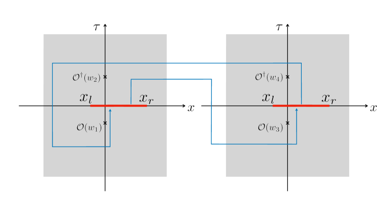
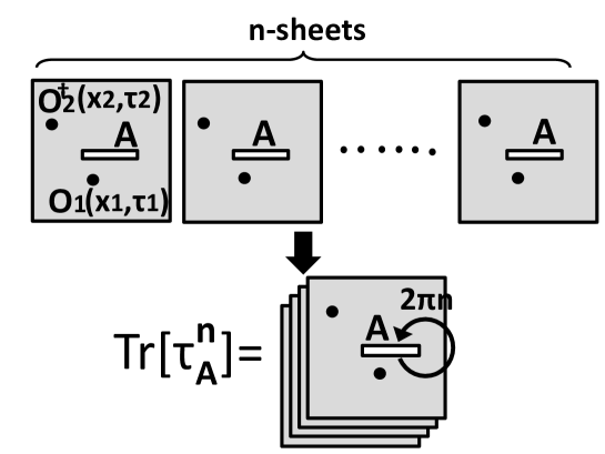
Figure 2: The replica method calculation of pseudo entropy in two dimensional CFTs for locally excited states.

We are interested in the difference between the pseudo Rényi entropy and the Rényi entropy of the ground state.

ΔSA(n)=S(n)(𝒯Aψ|φ)S(n)(ρA(0)),Δsubscriptsuperscript𝑆𝑛𝐴superscript𝑆𝑛subscriptsuperscript𝒯conditional𝜓𝜑𝐴superscript𝑆𝑛subscriptsuperscript𝜌0𝐴\Delta S^{(n)}_{A}=S^{(n)}(\mathcal{T}^{\psi|\varphi}_{A})-S^{(n)}(\rho^{(0)}_{A}), (2.36)

where ρA(0)=TrB|00|subscriptsuperscript𝜌0𝐴subscriptTr𝐵ket0bra0\rho^{(0)}_{A}=\mbox{Tr}_{B}\ket{0}\bra{0}, i.e. the reduced density matrix for the CFT vacuum.

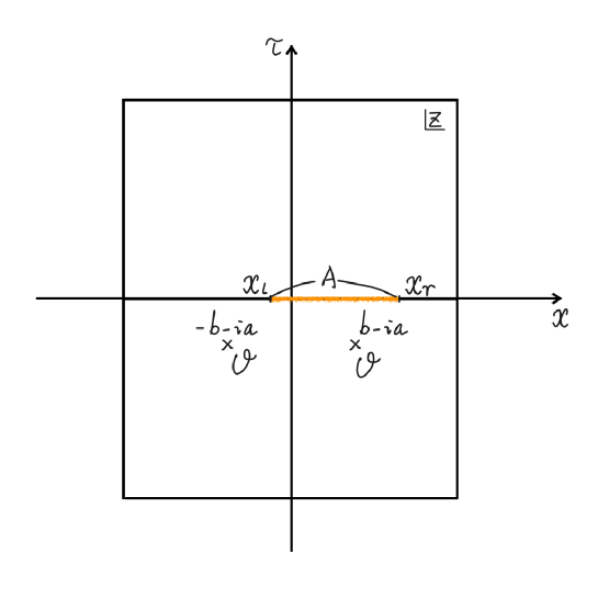
The trace Tr(𝒯Aψ|φ)nsuperscriptsubscriptsuperscript𝒯conditional𝜓𝜑𝐴𝑛(\mathcal{T}^{\psi|{\varphi}}_{A})^{n} can be obtained from the path-integral by gluing n𝑛n-sheets with two operators 𝒪𝒪\mathcal{O} and 𝒪superscript𝒪\mathcal{O}^{\dagger} inserted as shown in figure 2. We denote this replicated space as ΣnsubscriptΣ𝑛\Sigma_{n}. As in [27, 28] for the ordinary Rényi entropy via the replica method, we can calculate the difference (2.36) from the 2n2𝑛2n point function on ΣnsubscriptΣ𝑛\Sigma_{n} as follows

ΔSA(n)=11n[log𝒪(w1,w¯1)𝒪(w2,w¯2)𝒪(w2n,w¯2n)Σn(𝒪(w1,w¯1)𝒪(w2,w¯2)Σ1)n].Δsubscriptsuperscript𝑆𝑛𝐴11𝑛delimited-[]subscriptdelimited-⟨⟩superscript𝒪subscript𝑤1subscript¯𝑤1𝒪subscript𝑤2subscript¯𝑤2𝒪subscript𝑤2𝑛subscript¯𝑤2𝑛subscriptΣ𝑛superscriptsubscriptdelimited-⟨⟩superscript𝒪subscript𝑤1subscript¯𝑤1𝒪subscript𝑤2subscript¯𝑤2subscriptΣ1𝑛\displaystyle\Delta S^{(n)}_{A}=\frac{1}{1-n}\left[\log\frac{\langle\mathcal{O}^{\dagger}(w_{1},\bar{w}_{1})\mathcal{O}(w_{2},\bar{w}_{2})\cdot\cdot\cdot\mathcal{O}(w_{2n},\bar{w}_{2n})\rangle_{\Sigma_{n}}}{\left(\langle\mathcal{O}^{\dagger}(w_{1},\bar{w}_{1})\mathcal{O}(w_{2},\bar{w}_{2})\rangle_{\Sigma_{1}}\right)^{n}}\right]. (2.37)

We take wi=xi+iτisubscript𝑤𝑖subscript𝑥𝑖𝑖subscript𝜏𝑖w_{i}=x_{i}+i\tau_{i} to be the location of the operator insertion in each sheet. By applying the conformal map (we chose the subsystem A𝐴A to be an interval [xl,xr]subscript𝑥𝑙subscript𝑥𝑟[x_{l},x_{r}]),

wxlwxr=zn,𝑤subscript𝑥𝑙𝑤subscript𝑥𝑟superscript𝑧𝑛\displaystyle\frac{w-x_{l}}{w-x_{r}}=z^{n}, (2.38)

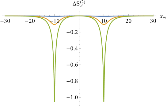
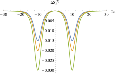
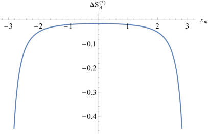
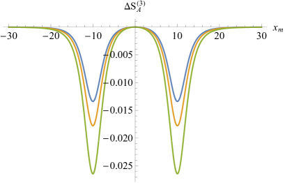
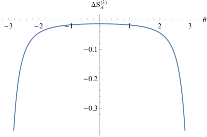
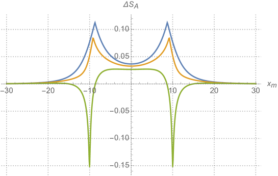
we can relate the above 2n2𝑛2n point function on ΣnsubscriptΣ𝑛\Sigma_{n} to that on a standard complex plane. We will evaluate ΔSA(n)Δsubscriptsuperscript𝑆𝑛𝐴\Delta S^{(n)}_{A} explicitly in section 4 for n=2,3𝑛23n=2,3. We will also present holographic pseudo entropy for such locally excited states in section 5.4.

2.5 Holographic Pseudo Entropy

As a special class of QFTs, holographic CFTs admit classical gravity duals via the AdS/CFT correspondence [14]. This allows us to compute the pseudo entropy holographically. Consider a computation of the inner product φ|ψinner-product𝜑𝜓\langle{\varphi}|\psi\rangle in the path-integral formalism of CFT. This quantity is identical to the partition function obtained by gluing along a time slice two Euclidean path-integrals, each of which produces |ψket𝜓|\psi\rangle and |φket𝜑|{\varphi}\rangle, respectively (depicted as the boundary of figure 1). If we insert operators O1(x1),O2(x2),subscript𝑂1subscript𝑥1subscript𝑂2subscript𝑥2O_{1}(x_{1}),O_{2}(x_{2}),\cdot\cdot\cdot on this time slice in this total path-integral, then we have (after dividing the inner product)

φ|O1(x1)O2(x2)|ψφ|ψ=Tr[𝒯ψ|φO1(x1)O2(x2)].quantum-operator-product𝜑subscript𝑂1subscript𝑥1subscript𝑂2subscript𝑥2𝜓inner-product𝜑𝜓Trdelimited-[]superscript𝒯conditional𝜓𝜑subscript𝑂1subscript𝑥1subscript𝑂2subscript𝑥2\displaystyle\frac{\langle{\varphi}|O_{1}(x_{1})O_{2}(x_{2})\cdot\cdot\cdot|\psi\rangle}{\langle{\varphi}|\psi\rangle}=\mbox{Tr}[{\mathcal{T}}^{\psi|{\varphi}}\cdot O_{1}(x_{1})O_{2}(x_{2})\cdot\cdot\cdot]. (2.39)

The AdS/CFT correspondence relates a d+1𝑑1d+1 dimensional gravity on an AdSd+1 to a d𝑑d dimensional holographic CFT. The gravity dual of this inner product is the classical partition function of an asymptotically AdS Euclidean space, which is obtained from the standard rule of the AdS/CFT. Note that since the bra and ket state on the time slice is different, there is neither (Euclidean) time-translational invariance nor the time reversal symmetry on the time slice. In this sense, we have the genuine Euclidean time-dependent geometry as the classical gravity dual.

Now we take a subsystem A𝐴A on the time slice in the holographic CFT and consider its (von Neumann) pseudo entropy S(𝒯Aψ|φ)𝑆subscriptsuperscript𝒯conditional𝜓𝜑𝐴S({\mathcal{T}}^{\psi|{\varphi}}_{A}). We argue that this is simply given by generalizing the holographic entanglement entropy [11, 12] to the gravity background with Euclidean time-dependence (refer to figure 1):

S(𝒯Aψ|φ)=MinΓA[A(ΓA)4GN],𝑆subscriptsuperscript𝒯conditional𝜓𝜑𝐴subscriptMinsubscriptΓ𝐴delimited-[]AsubscriptΓ𝐴4subscript𝐺𝑁\displaystyle S({\mathcal{T}}^{\psi|{\varphi}}_{A})=\mbox{Min}_{\Gamma_{A}}\left[\frac{\mbox{A}(\Gamma_{A})}{4G_{N}}\right], (2.40)

where ΓAsubscriptΓ𝐴\Gamma_{A} satisfies ΓA=AsubscriptΓ𝐴𝐴\partial\Gamma_{A}=\partial A and is homologous to A𝐴A.

Since it is straightforward to derive this formula as the authors of [20] did in the case of holographic entanglement entropy, here we give only a brief sketch of this. In the replica calculation explained in the previous subsection, we can obtain the n𝑛n-th pseudo Rényi entropy by computing TrA(TrB(|ψφ|))nsubscriptTr𝐴superscriptsubscriptTr𝐵ket𝜓bra𝜑𝑛\mathrm{Tr}_{A}\left(\mathrm{Tr}_{B}\left(|\psi\rangle\langle{\varphi}|\right)\right)^{n} as a partition function on n𝑛n-replicated geometry ΣnsubscriptΣ𝑛\Sigma_{n}. In this geometry, the deficit angle 2π(1n)2𝜋1𝑛2\pi(1-n) is present around the boundary of A𝐴A (i.e. A𝐴\partial A). In the AdS/CFT description, this partition function on ΣnsubscriptΣ𝑛\Sigma_{n} is equal to that of classical gravity on an asymptotically AdS space whose boundary coincides with the replicated space ΣnsubscriptΣ𝑛\Sigma_{n}. Naively the solution to Einstein equation with this boundary geometry is given by extending the deficit angle on A𝐴\partial A towards the bulk AdS. We call this extended surface with the deficit angle as ΓAsubscriptΓ𝐴\Gamma_{A}. However, the true solution to Einstein equation should be smooth and this deficit angle surface in the bulk, which is singular, is not an appropriate solution. Nevertheless, this naive prescription gives a correct von Neumann entropy (but not correct Rényi entropy). This is because the difference between the true solution and the singular solution is O(n1)𝑂𝑛1O(n-1) when n𝑛n is very closed to 111 and thus the values of the gravity action evaluated on these two solutions differ by O((n1)2)𝑂superscript𝑛12O\left((n-1)^{2}\right), which does not contribute in the von Neumann entropy limit n1𝑛1n\to 1. To see this, note that at n=1𝑛1n=1 the two solutions coincide with the standard AdS solution which satisfies the Einstein equation.

The gravity action takes the familiar form:

IG=116πGNdd+1xg(R2Λ)+,subscript𝐼𝐺116𝜋subscript𝐺𝑁superscript𝑑𝑑1𝑥𝑔𝑅2Λ\displaystyle I_{G}=-\frac{1}{16\pi G_{N}}\int d^{d+1}x\sqrt{g}\left(R-2\Lambda\right)+\cdot\cdot\cdot, (2.41)

where the omission \cdot\cdot\cdot includes the boundary term as well as matter field contributions which do not contribute to the entropy. In the presence of the deficit angle on ΓAsubscriptΓ𝐴\Gamma_{A}, the Ricci scalar behaves as R=4π(1n)δΓA(x)𝑅4𝜋1𝑛subscript𝛿subscriptΓ𝐴𝑥R=4\pi(1-n)\delta_{\Gamma_{A}}(x), where δΓA(x)subscript𝛿subscriptΓ𝐴𝑥\delta_{\Gamma_{A}}(x) is the delta-function which localizes on ΓAsubscriptΓ𝐴\Gamma_{A}. Therefore we can evaluate the O(n1)𝑂𝑛1O(n-1) term of the gravity action

IG=n14GNA(ΓA)+,subscript𝐼𝐺𝑛14subscript𝐺𝑁𝐴subscriptΓ𝐴\displaystyle I_{G}=\frac{n-1}{4G_{N}}A(\Gamma_{A})+\cdot\cdot\cdot, (2.42)

where the terms \cdot\cdot\cdot are all proportional to n𝑛n, which does not contribute to the entropy. The gravity partition function is expressed as ZG=eIGsubscript𝑍𝐺superscript𝑒subscript𝐼𝐺Z_{G}=e^{-I_{G}} in terms of the on-shell gravity action IGsubscript𝐼𝐺I_{G}. Finally the holographic pseudo entropy is computed as A(ΓA)4GN𝐴subscriptΓ𝐴4subscript𝐺𝑁\frac{A(\Gamma_{A})}{4G_{N}} by taking n1𝑛1n\to 1 limit of the formula (2.34). Solving Einstein equation corresponds to minimizing the area with respect to the change of ΓAsubscriptΓ𝐴\Gamma_{A}. These arguments derive the holographic formula (2.40).

Interestingly, this holographic formula tells us that the pseudo entropy computed for a classical gravity dual is always real and non-negative, assuming the bulk metric is real valued. This is because the only source for the holographic entanglement entropy by the replica trick is the Einstein Hilbert term which gives rise to the area term as in [20], as long as we consider Einstein gravity coupled to various matter fields. In the field theory side we can understand this as follows. Typically the Euclidean gravity with a real valued metric is dual to an Euclidean CFT with real valued external sources. In such a theory, the partition functions are positive and the same is true for Tr(𝒯Aψ|φ)nsuperscriptsubscriptsuperscript𝒯conditional𝜓𝜑𝐴𝑛(\mathcal{T}^{\psi|{\varphi}}_{A})^{n}. Also we expect the analyticity about the replica number n𝑛n, which can be confirmed in explicit results from CFT calculations in section 5.4. Therefore, we can compute the pseudo entropy without worrying about the choice of branch of the log function.

Notice also that the basic properties of (2.14), (2.15), and (2.16) are obvious in the holographic formula. Moreover, it is clear from the geometric property of asymptotically AdS backgrounds that the holographic pseudo entropy obeys the area law as in the standard entanglement entropy [6, 7]. We will give more details of holographic pseudo entropy with several examples in section 5.

We would like to mention that if we Wick rotate a generic Lorentzian time-dependent solution of Einstein gravity into an Euclidean time-dependent solution, we encounter a complex valued metric. In this case we expect the minimal area becomes complex valued. Though, in the present paper we will not discuss such cases, leaving it as a future problem, we would like to note that this looks consistent with the fact that the pseudo entropy is generically complex valued.

It is intriguing to compare this formula with the covariant holographic entanglement entropy [12], which calculates the entanglement entropy under time evolutions as the area of an extremal surface in a Lorentzian time-dependent asymptotically AdS spacetime. Our pseudo entropy formula in Euclidean asymptotically AdS spaces, may be regarded as a Wick rotation of the covariant holographic entanglement entropy from the gravity dual viewpoint. However, note that the former computes the von Neumann entropy for a standard quantum state, while the latter computes the von Neumann entropy for a transition matrix.

It is also useful to note that we can express the holographic pseudo entropy by using the area operator 𝒜^^𝒜\hat{\cal{A}} introduced in [29] as follows:

S(𝒯Aψ|φ)=φ|𝒜^4GN|ψφ|ψ,𝑆subscriptsuperscript𝒯conditional𝜓𝜑𝐴quantum-operator-product𝜑^𝒜4subscript𝐺𝑁𝜓inner-product𝜑𝜓\displaystyle S({\mathcal{T}}^{\psi|{\varphi}}_{A})=\frac{\langle{\varphi}|\frac{\hat{\cal{A}}}{4G_{N}}|\psi\rangle}{\langle{\varphi}|\psi\rangle}, (2.43)

i.e. the weak value of the area operator. We assume that |ψket𝜓|\psi\rangle and |φket𝜑|{\varphi}\rangle are in the same subspace of the low energy Hilbert space. Notice that if |ψket𝜓|\psi\rangle and |φket𝜑|{\varphi}\rangle are descendants of two different primaries, which are orthogonal to each other, then the φ|𝒜^|ψquantum-operator-product𝜑^𝒜𝜓\langle{\varphi}|\hat{\cal{A}}|\psi\rangle does vanish. Using this fact, we will confirm the expected linearity of the area operator in section 5.6.

3 Pseudo Entropy in Qubit Systems

In this section, we study pseudo entropy in qubit systems in detail.

3.1 Classification in 2-Qubit Systems

An arbitrary pure state in a 2-qubit system can be written as (up to an overall normalization)

|ψ=|00+a|11,(0a1)ket𝜓ket00𝑎ket110𝑎1\displaystyle\ket{\psi}=\ket{00}+a\ket{11},\leavevmode\nobreak\ \leavevmode\nobreak\ (0\leq a\leq 1) (3.1)

by choosing the basis appropriately. Here, we use the notation |ij|iA|jBket𝑖𝑗tensor-productsubscriptket𝑖𝐴subscriptket𝑗𝐵\ket{ij}\equiv|i\rangle_{A}\otimes|j\rangle_{B}. In such a basis, another arbitrary bipartite state can be written as (up to an overall normalization)

|φ=|00+beiθ|11+ceiξ|01+deiη|10,ket𝜑ket00𝑏superscript𝑒𝑖𝜃ket11𝑐superscript𝑒𝑖𝜉ket01𝑑superscript𝑒𝑖𝜂ket10\displaystyle\ket{{\varphi}}=\ket{00}+be^{-i\theta}\ket{11}+ce^{-i\xi}\ket{01}+de^{-i\eta}\ket{10}, (3.2)
(b,c,d0,πθ,ξ,ηπ).formulae-sequence𝑏𝑐𝑑0formulae-sequence𝜋𝜃𝜉𝜂𝜋\displaystyle(b,c,d\geq 0,\leavevmode\nobreak\ -\pi\leq\theta,\xi,\eta\leq\pi).

The transition matrix between the two states is reduced to

𝒯Aψ|φsubscriptsuperscript𝒯conditional𝜓𝜑𝐴\displaystyle{\mathcal{T}}^{\psi|{\varphi}}_{A} =11+abeiθ(|00|+aceiξ|10|+deiη|01|+abeiθ|11|)absent11𝑎𝑏superscript𝑒𝑖𝜃ket0quantum-operator-product0𝑎𝑐superscript𝑒𝑖𝜉1quantum-operator-product0𝑑superscript𝑒𝑖𝜂0quantum-operator-product1𝑎𝑏superscript𝑒𝑖𝜃1bra1\displaystyle=\frac{1}{1+abe^{i\theta}}\left(|0\rangle\langle 0|+ace^{i\xi}|1\rangle\langle 0|+de^{i\eta}|0\rangle\langle 1|+abe^{i\theta}|1\rangle\langle 1|\right)
(11+abeiθdeiη1+abeiθaceiξ1+abeiθabeiθ1+abeiθ)absentmatrix11𝑎𝑏superscript𝑒𝑖𝜃𝑑superscript𝑒𝑖𝜂1𝑎𝑏superscript𝑒𝑖𝜃𝑎𝑐superscript𝑒𝑖𝜉1𝑎𝑏superscript𝑒𝑖𝜃𝑎𝑏superscript𝑒𝑖𝜃1𝑎𝑏superscript𝑒𝑖𝜃\displaystyle\equiv\begin{pmatrix}{\frac{1}{1+abe^{i\theta}}}&{\frac{de^{i\eta}}{1+abe^{i\theta}}}\\ {\frac{ace^{i\xi}}{1+abe^{i\theta}}}&{\frac{abe^{i\theta}}{1+abe^{i\theta}}}\end{pmatrix} (3.3)

It is easy to see

𝒯ψ|φ𝒜 0det(𝒯Aψ|φ).superscript𝒯conditional𝜓𝜑𝒜 0subscriptsuperscript𝒯conditional𝜓𝜑𝐴\displaystyle{\mathcal{T}}^{\psi|{\varphi}}\in\mathscr{A}\leavevmode\nobreak\ \Longleftrightarrow\leavevmode\nobreak\ 0\leq\det{({\mathcal{T}}^{\psi|{\varphi}}_{A})}. (3.4)

It is also not hard to find that the following three statements are equivalent:

S(n)(𝒯Aψ|φ)takesnonnegativerealvaluesforn>0,i.e.𝒯ψ|φ.formulae-sequencesuperscript𝑆𝑛subscriptsuperscript𝒯conditional𝜓𝜑𝐴takesnonnegativerealvaluesfor𝑛0iesuperscript𝒯conditional𝜓𝜑\displaystyle S^{(n)}({\mathcal{T}}^{\psi|{\varphi}}_{A}){\rm\leavevmode\nobreak\ takes\leavevmode\nobreak\ nonnegative\leavevmode\nobreak\ real\leavevmode\nobreak\ values\leavevmode\nobreak\ for}\leavevmode\nobreak\ n>0{\rm,\leavevmode\nobreak\ i.e.\leavevmode\nobreak\ }{\mathcal{T}}^{\psi|{\varphi}}\in\mathscr{B}.
\displaystyle\Longleftrightarrow\leavevmode\nobreak\ Bothλ1andλ2arerealandnonnegative,i.e.𝒯ψ|φ𝒞.formulae-sequenceBothsubscript𝜆1andsubscript𝜆2arerealandnonnegativeiesuperscript𝒯conditional𝜓𝜑𝒞\displaystyle{\rm Both}\leavevmode\nobreak\ \lambda_{1}\leavevmode\nobreak\ {\rm and}\leavevmode\nobreak\ \lambda_{2}\leavevmode\nobreak\ {\rm are\leavevmode\nobreak\ real\leavevmode\nobreak\ and\leavevmode\nobreak\ nonnegative,\leavevmode\nobreak\ i.e.\leavevmode\nobreak\ }{\mathcal{T}}^{\psi|{\varphi}}\in\mathscr{C}. (3.5)
\displaystyle\Longleftrightarrow\leavevmode\nobreak\ 0det(𝒯Aψ|φ)1/4.0subscriptsuperscript𝒯conditional𝜓𝜑𝐴14\displaystyle 0\leq\det({\mathcal{T}}^{\psi|{\varphi}}_{A})\leq 1/4.

Let us then figure out when 𝒯ψ|φsuperscript𝒯conditional𝜓𝜑{\mathcal{T}}^{\psi|{\varphi}} gives positive semi-definite Hermitian 𝒯Aψ|φsubscriptsuperscript𝒯conditional𝜓𝜑𝐴{\mathcal{T}}^{\psi|{\varphi}}_{A}, i.e. 𝒯ψ|φ𝒟superscript𝒯conditional𝜓𝜑𝒟{\mathcal{T}}^{\psi|{\varphi}}\in\mathscr{D}. For two states |ψket𝜓\ket{\psi} and |φket𝜑\ket{{\varphi}} where

|ψ=|00+a|11,(0a1),ket𝜓ket00𝑎ket110𝑎1\displaystyle\ket{\psi}=\ket{00}+a\ket{11},\leavevmode\nobreak\ \leavevmode\nobreak\ (0\leq a\leq 1), (3.6)

𝒯Aψ|φsubscriptsuperscript𝒯conditional𝜓𝜑𝐴{\mathcal{T}}^{\psi|{\varphi}}_{A} is Hermitian if and only if

{b,b1/a0cπξπcasesformulae-sequence𝑏𝑏1𝑎otherwise0𝑐otherwise𝜋𝜉𝜋otherwise\displaystyle\exists\begin{cases}b\in\mathbb{R},b\neq-1/a\\ 0\leq c\\ -\pi\leq\xi\leq\pi\end{cases}
s.t.formulae-sequencest\displaystyle{\rm s.t.}
|φ=|00ket𝜑ket00\displaystyle\ket{{\varphi}}=\ket{00} +b|11+ceiξ|01+aceiξ|10.𝑏ket11𝑐superscript𝑒𝑖𝜉ket01𝑎𝑐superscript𝑒𝑖𝜉ket10\displaystyle+b\ket{11}+ce^{-i\xi}\ket{01}+ace^{i\xi}\ket{10}. (3.7)

In this case,

𝒯Aψ|φispositivesemidefinitea=0orbac2.subscriptsuperscript𝒯conditional𝜓𝜑𝐴ispositivesemidefinite𝑎0or𝑏𝑎superscript𝑐2\displaystyle{\mathcal{T}}^{\psi|{\varphi}}_{A}{\rm\leavevmode\nobreak\ is\leavevmode\nobreak\ positive\leavevmode\nobreak\ semi\mathchar 45\relax definite}\Longleftrightarrow\leavevmode\nobreak\ a=0\leavevmode\nobreak\ {\rm or}\leavevmode\nobreak\ b\geq ac^{2}. (3.8)

Note that 𝒯Aψ|φsubscriptsuperscript𝒯conditional𝜓𝜑𝐴{\mathcal{T}}^{\psi|{\varphi}}_{A} and 𝒯Bψ|φsubscriptsuperscript𝒯conditional𝜓𝜑𝐵{\mathcal{T}}^{\psi|{\varphi}}_{B} are not necessarily Hermitian at the same time. For two states |ψket𝜓\ket{\psi} and |φket𝜑\ket{{\varphi}} where

|ψ=|00+a|11,(0a1),ket𝜓ket00𝑎ket110𝑎1\displaystyle\ket{\psi}=\ket{00}+a\ket{11},\leavevmode\nobreak\ \leavevmode\nobreak\ (0\leq a\leq 1), (3.9)

both 𝒯Aψ|φsubscriptsuperscript𝒯conditional𝜓𝜑𝐴{\mathcal{T}}^{\psi|{\varphi}}_{A} and 𝒯Bψ|φsubscriptsuperscript𝒯conditional𝜓𝜑𝐵{\mathcal{T}}^{\psi|{\varphi}}_{B} are Hermitian if and only if it is either of the following two cases.
Case I: b,b1/aformulae-sequence𝑏𝑏1𝑎\exists b\in\mathbb{R},b\neq-1/a, s.t.

|φ=|00+b|11.ket𝜑ket00𝑏ket11\displaystyle\ket{{\varphi}}=\ket{00}+b\ket{11}. (3.10)

Case II: a=1𝑎1a=1 and

{b,b1/a0cπξπcasesformulae-sequence𝑏𝑏1𝑎otherwise0𝑐otherwise𝜋𝜉𝜋otherwise\displaystyle\exists\begin{cases}b\in\mathbb{R},b\neq-1/a\\ 0\leq c\\ -\pi\leq\xi\leq\pi\end{cases}
s.t.formulae-sequencest\displaystyle{\rm s.t.}
|φ=|00ket𝜑ket00\displaystyle\ket{{\varphi}}=\ket{00} +b|11+ceiξ|01+ceiξ|10.𝑏ket11𝑐superscript𝑒𝑖𝜉ket01𝑐superscript𝑒𝑖𝜉ket10\displaystyle+b\ket{11}+ce^{-i\xi}\ket{01}+ce^{i\xi}\ket{10}. (3.11)

In case I,

Both𝒯Aψ|φand𝒯Bψ|φarepositivesemidefinitea=0orb0.Bothsubscriptsuperscript𝒯conditional𝜓𝜑𝐴andsubscriptsuperscript𝒯conditional𝜓𝜑𝐵arepositivesemidefinite𝑎0or𝑏0\displaystyle{\rm Both}\leavevmode\nobreak\ {\mathcal{T}}^{\psi|{\varphi}}_{A}\leavevmode\nobreak\ {\rm and}\leavevmode\nobreak\ {\mathcal{T}}^{\psi|{\varphi}}_{B}\leavevmode\nobreak\ {\rm are\leavevmode\nobreak\ positive\leavevmode\nobreak\ semi\mathchar 45\relax definite}\leavevmode\nobreak\ \Longleftrightarrow\leavevmode\nobreak\ a=0\leavevmode\nobreak\ {\rm or}\leavevmode\nobreak\ b\geq 0. (3.12)

In case II,

Both𝒯Aψ|φand𝒯Bψ|φarepositivesemidefinitebc2.Bothsubscriptsuperscript𝒯conditional𝜓𝜑𝐴andsubscriptsuperscript𝒯conditional𝜓𝜑𝐵arepositivesemidefinite𝑏superscript𝑐2\displaystyle{\rm Both}\leavevmode\nobreak\ {\mathcal{T}}^{\psi|{\varphi}}_{A}\leavevmode\nobreak\ {\rm and}\leavevmode\nobreak\ {\mathcal{T}}^{\psi|{\varphi}}_{B}\leavevmode\nobreak\ {\rm are\leavevmode\nobreak\ positive\leavevmode\nobreak\ semi\mathchar 45\relax definite}\leavevmode\nobreak\ \Longleftrightarrow\leavevmode\nobreak\ b\geq c^{2}. (3.13)
Counting the Degrees of Freedom of 2-Qubit Transition Matrix

Choosing the basis like (3.1) and (3.2), it can be observed that there are 7 independent variables666We are counting the number of independent real variables which take continuous value. to characterize the transition matrix 𝒯ψ|φsuperscript𝒯conditional𝜓𝜑{\mathcal{T}}^{\psi|{\varphi}}. However, as we can see in (3.3), only 6 independent variables remain in 𝒯Aψ|φsubscriptsuperscript𝒯conditional𝜓𝜑𝐴{\mathcal{T}}^{\psi|{\varphi}}_{A}. Moreover, since the pseudo entropy can be computed from the two eigenvalues, there are only 2 independent variables that are relevant.

Considering transition matrices which give nonnegative real S(n)(𝒯Aψ|φ)superscript𝑆𝑛subscriptsuperscript𝒯conditional𝜓𝜑𝐴S^{(n)}({\mathcal{T}}^{\psi|{\varphi}}_{A}) for n>0𝑛0n>0, as we can see from (3.5), there are 6 independent variables for 𝒯ψ|φsuperscript𝒯conditional𝜓𝜑{\mathcal{T}}^{\psi|{\varphi}} and 5 independent variables for 𝒯Aψ|φsubscriptsuperscript𝒯conditional𝜓𝜑𝐴{\mathcal{T}}^{\psi|{\varphi}}_{A}.

If we focus on transition matrices which give positive semi-definite Hermitian 𝒯Aψ|φsubscriptsuperscript𝒯conditional𝜓𝜑𝐴{\mathcal{T}}^{\psi|{\varphi}}_{A}, according to (3.7) and (3.8), there are 4 independent variables for 𝒯ψ|φsuperscript𝒯conditional𝜓𝜑{\mathcal{T}}^{\psi|{\varphi}} and 3 independent variables for 𝒯Aψ|φsubscriptsuperscript𝒯conditional𝜓𝜑𝐴{\mathcal{T}}^{\psi|{\varphi}}_{A}.

Moreover, when both 𝒯Aψ|φsubscriptsuperscript𝒯conditional𝜓𝜑𝐴{\mathcal{T}}^{\psi|{\varphi}}_{A} and 𝒯Bψ|φsubscriptsuperscript𝒯conditional𝜓𝜑𝐵{\mathcal{T}}^{\psi|{\varphi}}_{B} are positive semi-definite Hermitian, the transition matrices can be classified in two cases. In case I, there are 2 independent variables for 𝒯ψ|φsuperscript𝒯conditional𝜓𝜑{\mathcal{T}}^{\psi|{\varphi}} and 1 independent variables for 𝒯Aψ|φsubscriptsuperscript𝒯conditional𝜓𝜑𝐴{\mathcal{T}}^{\psi|{\varphi}}_{A}. In case II, there are 3 independent variables for 𝒯ψ|φsuperscript𝒯conditional𝜓𝜑{\mathcal{T}}^{\psi|{\varphi}} and 3 independent variables for 𝒯Aψ|φsubscriptsuperscript𝒯conditional𝜓𝜑𝐴{\mathcal{T}}^{\psi|{\varphi}}_{A}.

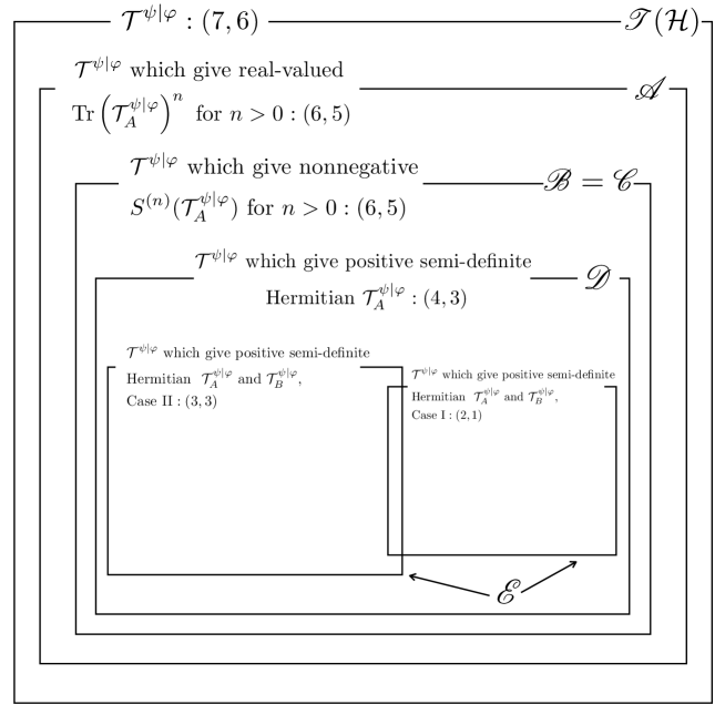
Figure 3 shows the Venn diagram of the classification of 2-qubit transition matrices we have discussed above.
Refer to caption
Figure 3: The Venn diagram of the classification of 2-qubit transition matrices. For each class of states, we use (m,n)𝑚𝑛(m,n) to represent that there are m𝑚m independent variables for 𝒯ψ|φsuperscript𝒯conditional𝜓𝜑{\mathcal{T}}^{\psi|{\varphi}} and n𝑛n independent variables for 𝒯Aψ|φsubscriptsuperscript𝒯conditional𝜓𝜑𝐴{\mathcal{T}}^{\psi|{\varphi}}_{A}.

Let us present an exotic example as follows, which belongs to the class 𝒜𝒜\mathscr{A} but not to \mathscr{B}.

Example 1.

For this we choose

|ψ=12(|00+eiθ|11),ket𝜓12ket00superscript𝑒𝑖𝜃ket11\displaystyle|\psi\rangle=\frac{1}{\sqrt{2}}(|00\rangle+e^{i\theta}|11\rangle),
|φ=12(|00+|11).ket𝜑12ket00ket11\displaystyle|{\varphi}\rangle=\frac{1}{\sqrt{2}}(|00\rangle+|11\rangle). (3.14)

We obtain

𝒯Aψ|φ=11+eiθ(|00|+eiθ|11|),subscriptsuperscript𝒯conditional𝜓𝜑𝐴11superscript𝑒𝑖𝜃ket0quantum-operator-product0superscript𝑒𝑖𝜃1bra1\displaystyle{\mathcal{T}}^{\psi|{\varphi}}_{A}=\frac{1}{1+e^{i\theta}}\left(|0\rangle\langle 0|+e^{i\theta}|1\rangle\langle 1|\right), (3.15)

where the eigenvalues are complex valued and each of them is complex conjugate to the other. We can evaluate the pseudo Rényi entropy

S(n)(𝒯Aψ|φ)=11nlog[cosnθ22n1cosn(θ2)].superscript𝑆𝑛subscriptsuperscript𝒯conditional𝜓𝜑𝐴11𝑛𝑛𝜃2superscript2𝑛1superscript𝑛𝜃2\displaystyle S^{(n)}({\mathcal{T}}^{\psi|{\varphi}}_{A})=\frac{1}{1-n}\log\left[\frac{\cos\frac{n\theta}{2}}{2^{n-1}\cos^{n}\left(\frac{\theta}{2}\right)}\right]. (3.16)

In particular for n=2𝑛2n=2, we find

S(2)(𝒯Aψ|φ)=log(1+cosθcosθ),superscript𝑆2subscriptsuperscript𝒯conditional𝜓𝜑𝐴1𝜃𝜃\displaystyle S^{(2)}({\mathcal{T}}^{\psi|{\varphi}}_{A})=\log\left(\frac{1+\cos\theta}{\cos\theta}\right), (3.17)

which is larger than log22\log 2 for 0<|θ|<π20𝜃𝜋20<|\theta|<\frac{\pi}{2} and is complex valued for π2<|θ|<π𝜋2𝜃𝜋\frac{\pi}{2}<|\theta|<\pi.

The pseudo von Neumann entropy reads

S(𝒯Aψ|φ)=log[2cosθ2]+θ2tanθ2.𝑆subscriptsuperscript𝒯conditional𝜓𝜑𝐴2𝜃2𝜃2𝜃2\displaystyle S({\mathcal{T}}^{\psi|{\varphi}}_{A})=\log\left[2\cos\frac{\theta}{2}\right]+\frac{\theta}{2}\cdot\tan\frac{\theta}{2}. (3.18)

Also note that, in this case, the two states |ψket𝜓\ket{\psi} and |φket𝜑\ket{{\varphi}} satisfy S(ρAψ)=S(ρAφ)𝑆subscriptsuperscript𝜌𝜓𝐴𝑆subscriptsuperscript𝜌𝜑𝐴S(\rho^{\psi}_{A})=S(\rho^{{\varphi}}_{A}) where ρAψ=TrB(|ψψ|)superscriptsubscript𝜌𝐴𝜓subscriptTr𝐵ket𝜓bra𝜓\rho_{A}^{\psi}=\mathrm{Tr}_{B}\left(|\psi\rangle\langle\psi|\right). We have

S(𝒯Aψ|φ)S(ρAψ)=S(𝒯Aψ|φ)S(ρAφ)𝑆subscriptsuperscript𝒯conditional𝜓𝜑𝐴𝑆subscriptsuperscript𝜌𝜓𝐴𝑆subscriptsuperscript𝒯conditional𝜓𝜑𝐴𝑆subscriptsuperscript𝜌𝜑𝐴\displaystyle S({\mathcal{T}}^{\psi|{\varphi}}_{A})-S(\rho^{\psi}_{A})=S({\mathcal{T}}^{\psi|{\varphi}}_{A})-S(\rho^{{\varphi}}_{A})
=\displaystyle= log[cosθ2]+θ2tanθ20.𝜃2𝜃2𝜃20\displaystyle\log\left[\cos\frac{\theta}{2}\right]+\frac{\theta}{2}\cdot\tan\frac{\theta}{2}\geq 0. (3.19)

However, note that the original periodicity of θ𝜃\theta disappears.

3.2 A Monotonicity of Pseudo Entropy in 2-Qubit Systems

Consider two states |ψket𝜓\ket{\psi} and |φket𝜑\ket{{\varphi}} in a 2-qubit system =ABtensor-productsubscript𝐴subscript𝐵{\mathcal{H}}={\mathcal{H}}_{A}\otimes{\mathcal{H}}_{B} which are related by a local basis transformation:

|ψ=(UV)|φket𝜓tensor-product𝑈𝑉ket𝜑\displaystyle\ket{\psi}=(U\otimes V)\ket{{\varphi}} (3.20)

where U𝑈U and V𝑉V are unitary transformations on Asubscript𝐴{\mathcal{H}}_{A} and Bsubscript𝐵{\mathcal{H}}_{B} respectively. A significant feature of 2-qubit systems in this setup is the following monotonicity under the unitary transformations:

S(n)(𝒯Aψ|φ)S(n)(TrB(|ψψ|))=S(n)(TrB(|φφ|))forn>0,formulae-sequencesuperscript𝑆𝑛subscriptsuperscript𝒯conditional𝜓𝜑𝐴superscript𝑆𝑛subscriptTr𝐵ket𝜓bra𝜓superscript𝑆𝑛subscriptTr𝐵ket𝜑bra𝜑for𝑛0\displaystyle S^{(n)}({\mathcal{T}}^{\psi|{\varphi}}_{A})\geq S^{(n)}(\mathrm{Tr}_{B}(|\psi\rangle\langle\psi|))=S^{(n)}(\mathrm{Tr}_{B}(|{\varphi}\rangle\langle{\varphi}|)){\leavevmode\nobreak\ \leavevmode\nobreak\ \rm for\leavevmode\nobreak\ \leavevmode\nobreak\ }n>0, (3.21)

if all the eigenvalues of 𝒯Aψ|φsubscriptsuperscript𝒯conditional𝜓𝜑𝐴{\mathcal{T}}^{\psi|{\varphi}}_{A} are real and nonnegative.

3.2.1 Proof

We present a proof by explicitly writing down the reduced transition matrix. We can always choose the basis such that

|ψ=c|0|0′′+s|1|1′′ket𝜓𝑐ketsuperscript0ketsuperscript0′′𝑠ketsuperscript1ketsuperscript1′′\displaystyle\ket{\psi}=c\ket{0^{\prime}}\ket{0^{\prime\prime}}+s\ket{1^{\prime}}\ket{1^{\prime\prime}} (3.22)
|φ=c|0|0+s|1|1ket𝜑𝑐ket0ket0𝑠ket1ket1\displaystyle\ket{{\varphi}}=c\ket{0}\ket{0}+s\ket{1}\ket{1} (3.23)

where 0sc10𝑠𝑐10\leq s\leq c\leq 1, c2+s2=1superscript𝑐2superscript𝑠21c^{2}+s^{2}=1 and,

|0=U|0,|1=U|1,formulae-sequenceketsuperscript0𝑈ket0ketsuperscript1𝑈ket1\displaystyle\ket{0^{\prime}}=U\ket{0},\leavevmode\nobreak\ \ket{1^{\prime}}=U\ket{1}, (3.24)
|0′′=V|0,|1′′=V|1.formulae-sequenceketsuperscript0′′𝑉ket0ketsuperscript1′′𝑉ket1\displaystyle\ket{0^{\prime\prime}}=V\ket{0},\leavevmode\nobreak\ \ket{1^{\prime\prime}}=V\ket{1}. (3.25)

Then,

|ψφ|ket𝜓bra𝜑\displaystyle|\psi\rangle\langle{\varphi}|
=\displaystyle= c2(U|00|)(V|00|)+cs(U|01|)(V|01|)tensor-productsuperscript𝑐2𝑈ket0bra0𝑉ket0bra0tensor-product𝑐𝑠𝑈ket0bra1𝑉ket0bra1\displaystyle\leavevmode\nobreak\ \leavevmode\nobreak\ c^{2}\left(U|0\rangle\langle 0|\right)\otimes\left(V|0\rangle\langle 0|\right)+cs\left(U|0\rangle\langle 1|\right)\otimes\left(V|0\rangle\langle 1|\right)
+cs(U|10|)(V|10|)+s2(U|11|)(V|11|).tensor-product𝑐𝑠𝑈ket1bra0𝑉ket1bra0tensor-productsuperscript𝑠2𝑈ket1bra1𝑉ket1bra1\displaystyle+cs\left(U|1\rangle\langle 0|\right)\otimes\left(V|1\rangle\langle 0|\right)+s^{2}\left(U|1\rangle\langle 1|\right)\otimes\left(V|1\rangle\langle 1|\right). (3.26)

Let us introduce the following notation:

M=M00|00|+M01|01|+M10|10|+M11|11|=(M00M01M10M11).𝑀subscript𝑀00ket0quantum-operator-product0subscript𝑀010quantum-operator-product1subscript𝑀101quantum-operator-product0subscript𝑀111bra1matrixsubscript𝑀00subscript𝑀01subscript𝑀10subscript𝑀11\displaystyle M=M_{00}|0\rangle\langle 0|+M_{01}|0\rangle\langle 1|+M_{10}|1\rangle\langle 0|+M_{11}|1\rangle\langle 1|=\begin{pmatrix}M_{00}&M_{01}\\ M_{10}&M_{11}\\ \end{pmatrix}. (3.27)

Tracing out the subsystem B𝐵B, we have

TrB(|ψφ|)=(c2V00U00+csV01U01s2V11U01+csV10U00c2V00U10+csV01U11s2V11U11+csV10U10).subscriptTr𝐵ket𝜓bra𝜑matrixsuperscript𝑐2subscript𝑉00subscript𝑈00𝑐𝑠subscript𝑉01subscript𝑈01superscript𝑠2subscript𝑉11subscript𝑈01𝑐𝑠subscript𝑉10subscript𝑈00superscript𝑐2subscript𝑉00subscript𝑈10𝑐𝑠subscript𝑉01subscript𝑈11superscript𝑠2subscript𝑉11subscript𝑈11𝑐𝑠subscript𝑉10subscript𝑈10\displaystyle\mathrm{Tr}_{B}\left(|\psi\rangle\langle{\varphi}|\right)=\begin{pmatrix}c^{2}V_{00}U_{00}+csV_{01}U_{01}&s^{2}V_{11}U_{01}+csV_{10}U_{00}\\ c^{2}V_{00}U_{10}+csV_{01}U_{11}&s^{2}V_{11}U_{11}+csV_{10}U_{10}\\ \end{pmatrix}. (3.28)

Thus we get the reduced transition matrix

𝒯Aψ|φ=1Δ(c2V00U00+csV01U01s2V11U01+csV10U00c2V00U10+csV01U11s2V11U11+csV10U10),subscriptsuperscript𝒯conditional𝜓𝜑𝐴1Δmatrixsuperscript𝑐2subscript𝑉00subscript𝑈00𝑐𝑠subscript𝑉01subscript𝑈01superscript𝑠2subscript𝑉11subscript𝑈01𝑐𝑠subscript𝑉10subscript𝑈00superscript𝑐2subscript𝑉00subscript𝑈10𝑐𝑠subscript𝑉01subscript𝑈11superscript𝑠2subscript𝑉11subscript𝑈11𝑐𝑠subscript𝑉10subscript𝑈10\displaystyle{\mathcal{T}}^{\psi|{\varphi}}_{A}=\frac{1}{\Delta}\begin{pmatrix}c^{2}V_{00}U_{00}+csV_{01}U_{01}&s^{2}V_{11}U_{01}+csV_{10}U_{00}\\ c^{2}V_{00}U_{10}+csV_{01}U_{11}&s^{2}V_{11}U_{11}+csV_{10}U_{10}\\ \end{pmatrix}, (3.29)

where

Δ=Tr(𝒯Aψ|φ)=c2V00U00+csV01U01+s2V11U11+csV10U10.ΔTrsubscriptsuperscript𝒯conditional𝜓𝜑𝐴superscript𝑐2subscript𝑉00subscript𝑈00𝑐𝑠subscript𝑉01subscript𝑈01superscript𝑠2subscript𝑉11subscript𝑈11𝑐𝑠subscript𝑉10subscript𝑈10\displaystyle\Delta=\mathrm{Tr}\left({\mathcal{T}}^{\psi|{\varphi}}_{A}\right)=c^{2}V_{00}U_{00}+csV_{01}U_{01}+s^{2}V_{11}U_{11}+csV_{10}U_{10}. (3.30)

It is sufficient to consider the situation in which U,VSU(2)𝑈𝑉SU2U,V\in{\rm SU(2)}. This allows us to have

U=(pqqp),V=(rttr)formulae-sequence𝑈matrix𝑝superscript𝑞𝑞superscript𝑝𝑉matrix𝑟superscript𝑡𝑡superscript𝑟\displaystyle U=\begin{pmatrix}p&-q^{*}\\ q&p^{*}\\ \end{pmatrix},\leavevmode\nobreak\ V=\begin{pmatrix}r&-t^{*}\\ t&r^{*}\\ \end{pmatrix} (3.31)

where |p|2+|q|2=|r|2+|t|2=1superscript𝑝2superscript𝑞2superscript𝑟2superscript𝑡21|p|^{2}+|q|^{2}=|r|^{2}+|t|^{2}=1. We then get

ΔΔ\displaystyle\Delta =c2pr+csqt+s2pr+csqtabsentsuperscript𝑐2𝑝𝑟𝑐𝑠superscript𝑞superscript𝑡superscript𝑠2superscript𝑝superscript𝑟𝑐𝑠𝑞𝑡\displaystyle=c^{2}pr+csq^{*}t^{*}+s^{2}p^{*}r^{*}+csqt
=Re(pr)+2csRe(qt)+i(c2s2)Im(pr)absentRe𝑝𝑟2𝑐𝑠Re𝑞𝑡𝑖superscript𝑐2superscript𝑠2Im𝑝𝑟\displaystyle={\rm Re}(pr)+2cs{\rm Re}(qt)+i(c^{2}-s^{2}){\rm Im}(pr) (3.32)

and

det𝒯Aψ|φ=c2s2Δ2.subscriptsuperscript𝒯conditional𝜓𝜑𝐴superscript𝑐2superscript𝑠2superscriptΔ2\displaystyle\det{{\mathcal{T}}^{\psi|{\varphi}}_{A}}=\frac{c^{2}s^{2}}{\Delta^{2}}. (3.33)

The two eigenvalues of 𝒯Aψ|φsubscriptsuperscript𝒯conditional𝜓𝜑𝐴{\mathcal{T}}^{\psi|{\varphi}}_{A} are the two solutions of

F(λ)λ2λ+c2s2Δ2=0.𝐹𝜆superscript𝜆2𝜆superscript𝑐2superscript𝑠2superscriptΔ20\displaystyle F(\lambda)\equiv\lambda^{2}-\lambda+\frac{c^{2}s^{2}}{\Delta^{2}}=0. (3.34)

We denote them as λλ+subscript𝜆subscript𝜆\lambda_{-}\leq\lambda_{+}. Both λsubscript𝜆\lambda_{-} and λ+subscript𝜆\lambda_{+} are real and nonnegative if and only if

0c2s2Δ214.0superscript𝑐2superscript𝑠2superscriptΔ214\displaystyle 0\leq\frac{c^{2}s^{2}}{\Delta^{2}}\leq\frac{1}{4}. (3.35)

In this case ΔΔ\Delta\in\mathbb{R} and hence

|Δ|Δ\displaystyle|\Delta| =|Re(pr)+2csRe(qt)|absentRe𝑝𝑟2𝑐𝑠Re𝑞𝑡\displaystyle=|{\rm Re}(pr)+2cs{\rm Re}(qt)|
|Re(pr)|+2cs|Re(qt)|absentRe𝑝𝑟2𝑐𝑠Re𝑞𝑡\displaystyle\leq|{\rm Re}(pr)|+2cs|{\rm Re}(qt)|
|Re(pr)|+(c2+s2)|Re(qt)|absentRe𝑝𝑟superscript𝑐2superscript𝑠2Re𝑞𝑡\displaystyle\leq|{\rm Re}(pr)|+(c^{2}+s^{2})|{\rm Re}(qt)|
=|Re(pr)|+|Re(qt)|absentRe𝑝𝑟Re𝑞𝑡\displaystyle=|{\rm Re}(pr)|+|{\rm Re}(qt)|
|p||r|+|q||t|absent𝑝𝑟𝑞𝑡\displaystyle\leq|p||r|+|q||t|
=cos(αβ)1.absent𝛼𝛽1\displaystyle=\cos(\alpha-\beta)\leq 1. (3.36)

where in the last line we recognize |p|=cosα,|q|=sinα,|r|=cosβ,|t|=sinβformulae-sequence𝑝𝛼formulae-sequence𝑞𝛼formulae-sequence𝑟𝛽𝑡𝛽|p|=\cos\alpha,\leavevmode\nobreak\ |q|=\sin\alpha,\leavevmode\nobreak\ |r|=\cos\beta,\leavevmode\nobreak\ |t|=\sin\beta. Let us go back to our statement (3.21). Under the condition that the eigenvalues of 𝒯Aψ|φsubscriptsuperscript𝒯conditional𝜓𝜑𝐴{\mathcal{T}}^{\psi|{\varphi}}_{A} are real and positive,

S(n)(𝒯Aψ|φ)S(n)(TrB(|ψψ|))=S(n)(TrB(|φφ|))forn>0formulae-sequencesuperscript𝑆𝑛subscriptsuperscript𝒯conditional𝜓𝜑𝐴superscript𝑆𝑛subscriptTr𝐵ket𝜓bra𝜓superscript𝑆𝑛subscriptTr𝐵ket𝜑bra𝜑for𝑛0\displaystyle S^{(n)}({\mathcal{T}}^{\psi|{\varphi}}_{A})\geq S^{(n)}(\mathrm{Tr}_{B}(|\psi\rangle\langle\psi|))=S^{(n)}(\mathrm{Tr}_{B}(|{\varphi}\rangle\langle{\varphi}|)){\leavevmode\nobreak\ \leavevmode\nobreak\ \rm for\leavevmode\nobreak\ \leavevmode\nobreak\ }n>0
\displaystyle\Longleftrightarrow\leavevmode\nobreak\ 0s2λλ+c21(Majorization[30])formulae-sequence0superscript𝑠2subscript𝜆subscript𝜆superscript𝑐21Majorization[30]\displaystyle 0\leq s^{2}\leq\lambda_{-}\leq\lambda_{+}\leq c^{2}\leq 1\leavevmode\nobreak\ \leavevmode\nobreak\ {\rm(Majorization\cite[cite]{[\@@bibref{}{Nielsen98}{}{}]})}
\displaystyle\Longleftrightarrow\leavevmode\nobreak\ F(c2)=c2s2(1Δ21)0,𝐹superscript𝑐2superscript𝑐2superscript𝑠21superscriptΔ210\displaystyle F(c^{2})=c^{2}s^{2}\left(\frac{1}{\Delta^{2}}-1\right)\geq 0, (3.37)

and the last line follows directly from (3.36).

3.2.2 Beyond Two Qubits

We would like to note that the same statement is not true in general Hilbert space. Let us see a representative example in 2-qutrit systems.

Example 2.

Consider the following two states.

|ψ=12(|0|0+|1|1),ket𝜓12ket0ket0ket1ket1\displaystyle\ket{\psi}=\frac{1}{\sqrt{2}}\left(\ket{0}\ket{0}+\ket{1}\ket{1}\right), (3.38)
|φ=12(|0|0+|1|2).ket𝜑12ket0ket0ket1ket2\displaystyle\ket{{\varphi}}=\frac{1}{\sqrt{2}}\left(\ket{0}\ket{0}+\ket{1}\ket{2}\right). (3.39)

The two states are related by a local basis transformation and

S(n)(TrB(|ψψ|))=S(n)(TrB(|φφ|))=log2forn>0.formulae-sequencesuperscript𝑆𝑛subscriptTr𝐵ket𝜓bra𝜓superscript𝑆𝑛subscriptTr𝐵ket𝜑bra𝜑2for𝑛0\displaystyle S^{(n)}(\mathrm{Tr}_{B}(|\psi\rangle\langle\psi|))=S^{(n)}(\mathrm{Tr}_{B}(|{\varphi}\rangle\langle{\varphi}|))=\log 2{\leavevmode\nobreak\ \leavevmode\nobreak\ \rm for\leavevmode\nobreak\ \leavevmode\nobreak\ }n>0. (3.40)

On the other hand,

𝒯Aψ|φ=(100000000),𝒯Bψ|φ=(100001000).formulae-sequencesubscriptsuperscript𝒯conditional𝜓𝜑𝐴matrix100000000subscriptsuperscript𝒯conditional𝜓𝜑𝐵matrix100001000\displaystyle{\mathcal{T}}^{\psi|{\varphi}}_{A}=\begin{pmatrix}1&0&0\\ 0&0&0\\ 0&0&0\end{pmatrix},{\mathcal{T}}^{\psi|{\varphi}}_{B}=\begin{pmatrix}1&0&0\\ 0&0&1\\ 0&0&0\end{pmatrix}. (3.41)

and hence

S(n)(𝒯Aψ|φ)=0<log2=S(n)(TrB(|ψψ|))=S(n)(TrB(|φφ|))forn>0.formulae-sequencesuperscript𝑆𝑛subscriptsuperscript𝒯conditional𝜓𝜑𝐴02superscript𝑆𝑛subscriptTr𝐵ket𝜓bra𝜓superscript𝑆𝑛subscriptTr𝐵ket𝜑bra𝜑for𝑛0\displaystyle S^{(n)}({\mathcal{T}}^{\psi|{\varphi}}_{A})=0<\log 2=S^{(n)}(\mathrm{Tr}_{B}(|\psi\rangle\langle\psi|))=S^{(n)}(\mathrm{Tr}_{B}(|{\varphi}\rangle\langle{\varphi}|)){\leavevmode\nobreak\ \leavevmode\nobreak\ \rm for\leavevmode\nobreak\ \leavevmode\nobreak\ }n>0. (3.42)

The third dimension plays a crucial role in the distinguishment from 2-qubit cases.

It is easy to understand this difference between 2-qubit systems and higher dimensional systems. Let us denote the eigenvalues of TrB(|φφ|)subscriptTr𝐵ket𝜑bra𝜑{\rm Tr}_{B}\left(|{\varphi}\rangle\langle{\varphi}|\right) as a>b>c𝑎𝑏𝑐a>b>c. Now in this case the local unitary transformation only changes the eigenspace corresponding to b𝑏b and c𝑐c. Therefore, by using the result in the 2-qubit case, the eigenvalues change toward majorization[30]. On the other hand, if we take the normalization into consideration and look at the whole Hilbert space, we can see that the normalization changes the eigenvalues toward an opposite direction of majorization. As a result, we cannot justify whether S(n)(𝒯Aψ|φ)superscript𝑆𝑛subscriptsuperscript𝒯conditional𝜓𝜑𝐴S^{(n)}({\mathcal{T}}^{\psi|{\varphi}}_{A}) is larger than S(n)(TrB(|ψψ|))=S(n)(TrB(|φφ|))superscript𝑆𝑛subscriptTr𝐵ket𝜓bra𝜓superscript𝑆𝑛subscriptTr𝐵ket𝜑bra𝜑S^{(n)}(\mathrm{Tr}_{B}(|\psi\rangle\langle\psi|))=S^{(n)}(\mathrm{Tr}_{B}(|{\varphi}\rangle\langle{\varphi}|)) in general.

We also would like to point out a closely related example in 4-qubit system:

Example 3.

Consider a 4-qubit system, where the qubits are denoted by A1,A2,B1subscript𝐴1subscript𝐴2subscript𝐵1A_{1},A_{2},B_{1} and B2subscript𝐵2B_{2}, respectively. We regard the first two qubits as A𝐴A i.e. A=A1A2𝐴subscript𝐴1subscript𝐴2A=A_{1}A_{2} and similarly for the latter two qubits B=B1B2𝐵subscript𝐵1subscript𝐵2B=B_{1}B_{2}. For the states

|ψ=(|0000+|0110)/2,ket𝜓ket0000ket01102\displaystyle\ket{\psi}=(\ket{0000}+\ket{0110})/\sqrt{2}, (3.43)
|φ=(|0000+|1001)/2,ket𝜑ket0000ket10012\displaystyle\ket{{\varphi}}=(\ket{0000}+\ket{1001})/\sqrt{2}, (3.44)

it is straightforward to see S(𝒯Aψ|φ)=0𝑆subscriptsuperscript𝒯conditional𝜓𝜑𝐴0S({\mathcal{T}}^{\psi|{\varphi}}_{A})=0 and S(TrB(|ψψ|))=S(TrB(|φφ|))=log2𝑆subscriptTr𝐵ket𝜓bra𝜓𝑆subscriptTr𝐵ket𝜑bra𝜑2S(\mathrm{Tr}_{B}(|\psi\rangle\langle\psi|))=S(\mathrm{Tr}_{B}(|{\varphi}\rangle\langle{\varphi}|))=\log 2. In this example, |φket𝜑\ket{{\varphi}} is obtained from |ψket𝜓\ket{\psi} by replacing the Bell pair of A2B1subscript𝐴2subscript𝐵1A_{2}B_{1} with that of A1B2subscript𝐴1subscript𝐵2A_{1}B_{2}. This implies the entanglement swapping (or transition) reduces the values of pseudo entropy compared with the original amount of quantum entanglement for each of states.

Moreover, as we discuss in appendix B for thermofield double states and appendix C for two coupled harmonic oscillators, we can find physical examples with larger degrees of freedom which tend to satisfy the opposite inequality, namely, the pseudo entropy gets smaller than the averaged original entanglement entropy.

3.2.3 A Weaker Inequality

Nevertheless, we would like to mention that in general Hilbert spaces, a weaker bound can be obtained. We consider

|ψ=(U1)|φket𝜓tensor-product𝑈1ket𝜑\displaystyle\ket{\psi}=(U\otimes 1)\ket{{\varphi}} (3.45)

where the unitary transformation U𝑈U only acts on the Hilbert space Asubscript𝐴\mathcal{H}_{A}. We assume Asubscript𝐴\mathcal{H}_{A} and Bsubscript𝐵\mathcal{H}_{B} are arbitrary and |φABket𝜑tensor-productsubscript𝐴subscript𝐵\ket{{\varphi}}\in\mathcal{H}_{A}\otimes\mathcal{H}_{B} can be any quantum state. In this setup, if we set ρφ=TrB|φφ|subscript𝜌𝜑subscriptTr𝐵ket𝜑bra𝜑\rho_{\varphi}=\mbox{Tr}_{B}|{\varphi}\rangle\langle{\varphi}|, then the transition matrix looks like

𝒯Aψ|φ=UρφTr[Uρφ].subscriptsuperscript𝒯conditional𝜓𝜑𝐴𝑈subscript𝜌𝜑Trdelimited-[]𝑈subscript𝜌𝜑\displaystyle{\mathcal{T}}^{\psi|{\varphi}}_{A}=\frac{U\cdot\rho_{\varphi}}{\mbox{Tr}[U\cdot\rho_{\varphi}]}. (3.46)

By writing the eigenvalues of ρAφsubscriptsuperscript𝜌𝜑𝐴\rho^{\varphi}_{A} and UρAφ𝑈subscriptsuperscript𝜌𝜑𝐴U\cdot\rho^{\varphi}_{A} as {σi}subscript𝜎𝑖\{\sigma_{i}\} and {λi}subscript𝜆𝑖\{\lambda_{i}\} in decreasing order, respectively, the Weyl’s inequality leads to the relation

i=1k|λi|pi=1k(σi)p,superscriptsubscript𝑖1𝑘superscriptsubscript𝜆𝑖𝑝superscriptsubscript𝑖1𝑘superscriptsubscript𝜎𝑖𝑝\displaystyle\sum_{i=1}^{k}|\lambda_{i}|^{p}\leq\sum_{i=1}^{k}(\sigma_{i})^{p}, (3.47)

for any k(dimA)annotated𝑘absentdimsubscript𝐴k(\leq\mbox{dim}\mathcal{H}_{A}).

If we assume the eigenvalues of UρAφ𝑈subscriptsuperscript𝜌𝜑𝐴U\cdot\rho^{\varphi}_{A} are real and non-negative, then the above inequality gives the weaker bound:

S(n)(𝒯Aψ|φ)S(n)(ρAφ)+nn1logφ|ψ.superscript𝑆𝑛subscriptsuperscript𝒯conditional𝜓𝜑𝐴superscript𝑆𝑛subscriptsuperscript𝜌𝜑𝐴𝑛𝑛1inner-product𝜑𝜓\displaystyle S^{(n)}({\mathcal{T}}^{\psi|{\varphi}}_{A})\geq S^{(n)}(\rho^{\varphi}_{A})+\frac{n}{n-1}\log\langle{\varphi}|\psi\rangle. (3.48)

3.3 Pseudo Entropy as Number of Bell Pairs in Class \mathscr{E}

In this subsection we would like to present an interpretation of pseudo entropy as a number of Bell pairs included in intermediate states by focusing on the class \mathscr{E}, which is supposed to be least exotic.777 Even though there are case I and case II in class \mathscr{E} (see Fig.3), the case II can be reduced to case I via unitary transformation of the basis. Therefore we can focus on the case I..

For this, let us consider the following states:

Example 4.

We choose the two quantum states as follows

|ψ1AB=cosθ1|00AB+sinθ1|11AB,subscriptketsubscript𝜓1𝐴𝐵subscript𝜃1subscriptket00𝐴𝐵subscript𝜃1subscriptket11𝐴𝐵\displaystyle|\psi_{1}\rangle_{AB}=\cos\theta_{1}|00\rangle_{AB}+\sin\theta_{1}|11\rangle_{AB},
|ψ2AB=cosθ2|00AB+sinθ2|11AB.subscriptketsubscript𝜓2𝐴𝐵subscript𝜃2subscriptket00𝐴𝐵subscript𝜃2subscriptket11𝐴𝐵\displaystyle|\psi_{2}\rangle_{AB}=\cos\theta_{2}|00\rangle_{AB}+\sin\theta_{2}|11\rangle_{AB}. (3.49)

We assume 0θ1,θ2π2formulae-sequence0subscript𝜃1subscript𝜃2𝜋20\leq\theta_{1},\theta_{2}\leq\frac{\pi}{2} or π2θ1,θ2πformulae-sequence𝜋2subscript𝜃1subscript𝜃2𝜋\frac{\pi}{2}\leq\theta_{1},\theta_{2}\leq\pi in order to be in class 𝒟𝒟\mathscr{D} (i.e. 𝒯Aψ1|ψ2subscriptsuperscript𝒯conditionalsubscript𝜓1subscript𝜓2𝐴{\mathcal{T}}^{\psi_{1}|\psi_{2}}_{A} is positive semi-definite Hermitian matrix). The reduced density matrix in each state reads

ρA(i)=cos2θi|00|+sin2θi|11|.(i=1,2)\displaystyle\rho^{(i)}_{A}=\cos^{2}\theta_{i}|0\rangle\langle 0|+\sin^{2}\theta_{i}|1\rangle\langle 1|.\ \ \ (i=1,2) (3.50)

The entanglement entropy for each state is found as

S(ρA(i))=cos2θilogcos2θisin2θilogsin2θi,(i=1,2).𝑆subscriptsuperscript𝜌𝑖𝐴superscript2subscript𝜃𝑖superscript2subscript𝜃𝑖superscript2subscript𝜃𝑖superscript2subscript𝜃𝑖𝑖12\displaystyle S(\rho^{(i)}_{A})=-\cos^{2}\theta_{i}\log\cos^{2}\theta_{i}-\sin^{2}\theta_{i}\log\sin^{2}\theta_{i},\ \ \ (i=1,2). (3.51)

The transition matrix is found as

𝒯Aψ1|ψ2=1cos(θ1θ2)(cosθ1cosθ2|00|+sinθ1sinθ2|11|).subscriptsuperscript𝒯conditionalsubscript𝜓1subscript𝜓2𝐴1subscript𝜃1subscript𝜃2subscript𝜃1subscript𝜃2ket0quantum-operator-product0subscript𝜃1subscript𝜃21bra1\displaystyle\mathcal{T}^{\psi_{1}|\psi_{2}}_{A}=\frac{1}{\cos(\theta_{1}-\theta_{2})}(\cos\theta_{1}\cos\theta_{2}|0\rangle\langle 0|+\sin\theta_{1}\sin\theta_{2}|1\rangle\langle 1|). (3.52)

The pseudo Rényi entropy is computed as

S(n)(𝒯Aψ1|ψ2)=11nlog[(cosθ1cosθ2cos(θ1θ2))n+(sinθ1sinθ2cos(θ1θ2))n].superscript𝑆𝑛subscriptsuperscript𝒯conditionalsubscript𝜓1subscript𝜓2𝐴11𝑛superscriptsubscript𝜃1subscript𝜃2subscript𝜃1subscript𝜃2𝑛superscriptsubscript𝜃1subscript𝜃2subscript𝜃1subscript𝜃2𝑛\displaystyle S^{(n)}(\mathcal{T}^{\psi_{1}|\psi_{2}}_{A})=\frac{1}{1-n}\log\left[\left(\frac{\cos\theta_{1}\cos\theta_{2}}{\cos(\theta_{1}-\theta_{2})}\right)^{n}+\left(\frac{\sin\theta_{1}\sin\theta_{2}}{\cos(\theta_{1}-\theta_{2})}\right)^{n}\right]. (3.53)

The entanglement pseudo entropy is found as

S(𝒯Aψ1|ψ2)=𝑆subscriptsuperscript𝒯conditionalsubscript𝜓1subscript𝜓2𝐴absent\displaystyle S(\mathcal{T}^{\psi_{1}|\psi_{2}}_{A})= (cosθ1cosθ2cos(θ1θ2))log(cosθ1cosθ2cos(θ1θ2))subscript𝜃1subscript𝜃2subscript𝜃1subscript𝜃2subscript𝜃1subscript𝜃2subscript𝜃1subscript𝜃2\displaystyle-\left(\frac{\cos\theta_{1}\cos\theta_{2}}{\cos(\theta_{1}-\theta_{2})}\right)\cdot\log\left(\frac{\cos\theta_{1}\cos\theta_{2}}{\cos(\theta_{1}-\theta_{2})}\right) (3.54)
(sinθ1sinθ2cos(θ1θ2))log(sinθ1sinθ2cos(θ1θ2)).subscript𝜃1subscript𝜃2subscript𝜃1subscript𝜃2subscript𝜃1subscript𝜃2subscript𝜃1subscript𝜃2\displaystyle\ \ -\left(\frac{\sin\theta_{1}\sin\theta_{2}}{\cos(\theta_{1}-\theta_{2})}\right)\cdot\log\left(\frac{\sin\theta_{1}\sin\theta_{2}}{\cos(\theta_{1}-\theta_{2})}\right).

This is plotted in the left picture of Fig.4.

When θ1=θ2subscript𝜃1subscript𝜃2\theta_{1}=\theta_{2}, this is reduced to the ordinary entanglement entropy (3.51). Moreover, when θ1+θ2=π2(2m+1)subscript𝜃1subscript𝜃2𝜋22𝑚1\theta_{1}+\theta_{2}=\frac{\pi}{2}(2m+1) (here m𝑚m is an integer), we always find S(𝒯Aψ1|ψ2)=log2𝑆subscriptsuperscript𝒯conditionalsubscript𝜓1subscript𝜓2𝐴2S(\mathcal{T}^{\psi_{1}|\psi_{2}}_{A})=\log 2. This is intriguing because even though the entanglement entropies for |ψ1ketsubscript𝜓1|\psi_{1}\rangle and |ψ2ketsubscript𝜓2|\psi_{2}\rangle are small, the pseudo entropy can be large.

It is useful to note that the following difference which measures such an enhancement:

S(𝒯Aψ1|ψ2)12(S(ρA(1))+S(ρA(2)))𝑆subscriptsuperscript𝒯conditionalsubscript𝜓1subscript𝜓2𝐴12𝑆subscriptsuperscript𝜌1𝐴𝑆subscriptsuperscript𝜌2𝐴\displaystyle S(\mathcal{T}^{\psi_{1}|\psi_{2}}_{A})-\frac{1}{2}(S(\rho^{(1)}_{A})+S(\rho^{(2)}_{A})) (3.55)

can be both positive and negative in general as in the right picture of Fig.4.
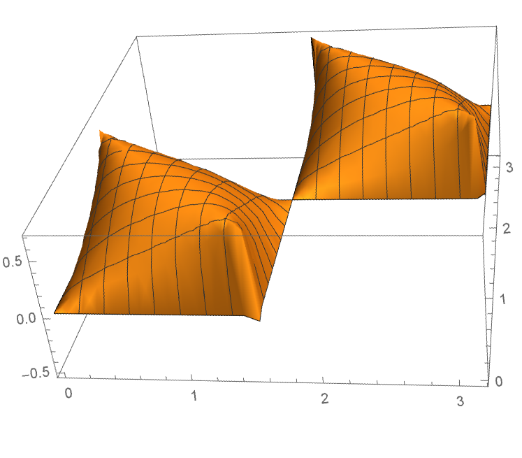
Refer to caption Refer to caption
Figure 4: We plot the pseudo entropy for the two qubit system as a function θ1subscript𝜃1\theta_{1} (horizontal axis) and θ2subscript𝜃2\theta_{2} (depth axis) in the left graph. The right one shows the pseudo entropy minus the averaged entanglement entropy i.e. (3.55). We took the range 0θ1,2π0subscript𝜃12𝜋0\leq\theta_{1,2}\leq\pi. The region where no graph is shown gives complex valued pseudo entropy.

3.3.1 Interpretation via Quantum Entanglement

Now let us consider an interpretation of pseudo entropy from the view point of quantum entanglement by extending the well-known argument [30, 31] for the entanglement entropy. Again we assume two quantum states are in the form (3.49). We regard |ψ1ketsubscript𝜓1|\psi_{1}\rangle as the initial state and |ψ2ketsubscript𝜓2|\psi_{2}\rangle as the final state of the post-selection. We would like to estimate the averaged number of Bell pairs that could have been potentially distilled from intermediate states before the state was actually post-selected. More specifically, we rewrite ψ2|ψ1inner-productsubscript𝜓2subscript𝜓1\langle\psi_{2}|\psi_{1}\rangle as nψ2|nn|ψ1subscript𝑛inner-productsubscript𝜓2𝑛inner-product𝑛subscript𝜓1\sum_{n}\langle\psi_{2}|n\rangle\langle n|\psi_{1}\rangle and consider the number of Bell pairs that can be distilled from the intermediate state |nket𝑛|n\rangle. Since the state would have appeared with probability pn=(ψ2|nn|ψ1)/ψ2|ψ1subscript𝑝𝑛inner-productsubscript𝜓2𝑛inner-product𝑛subscript𝜓1inner-productsubscript𝜓2subscript𝜓1p_{n}=(\langle\psi_{2}|n\rangle\langle n|\psi_{1}\rangle)/\langle\psi_{2}|\psi_{1}\rangle, we take the average over pnsubscript𝑝𝑛p_{n}. This protocol is obviously not real since the post-selected state is |ψ2ketsubscript𝜓2\ket{\psi_{2}}, but not |nket𝑛\ket{n}. We however think that this quantity is worth studying from a theoretical viewpoint since the quantity allows us to assess the amount of entanglement that is virtually involved in the post-selection process.

Motivated by the LOCC interpretation of entanglement entropy we would like to take the asymptotic limit and consider the M𝑀M replicated states

|ψiM=(ci|00+si|11)M,superscriptketsubscript𝜓𝑖tensor-productabsent𝑀superscriptsubscript𝑐𝑖ket00subscript𝑠𝑖ket11tensor-productabsent𝑀\displaystyle|\psi_{i}\rangle^{\otimes M}=(c_{i}|00\rangle+s_{i}|11\rangle)^{\otimes M}, (3.56)

where we defined ci=cosθisubscript𝑐𝑖subscript𝜃𝑖c_{i}=\cos\theta_{i} and si=sinθisubscript𝑠𝑖subscript𝜃𝑖s_{i}=\sin\theta_{i}. This is expanded in the form:

|ψiM=k=0MciMksika=1CkM|Pa(k)A|Pa(k)B,(i=1,2)superscriptketsubscript𝜓𝑖tensor-productabsent𝑀superscriptsubscript𝑘0𝑀superscriptsubscript𝑐𝑖𝑀𝑘superscriptsubscript𝑠𝑖𝑘superscriptsubscript𝑎1subscriptsubscript𝐶𝑘𝑀subscriptketsubscriptsuperscript𝑃𝑘𝑎𝐴subscriptketsubscriptsuperscript𝑃𝑘𝑎𝐵𝑖12\displaystyle|\psi_{i}\rangle^{\otimes M}=\sum_{k=0}^{M}c_{i}^{M-k}s_{i}^{k}\sum_{a=1}^{{}_{M}C_{k}}|P^{(k)}_{a}\rangle_{A}|P^{(k)}_{a}\rangle_{B},\ \ (i=1,2) (3.57)

where CkM=M!(Mk)!k!subscriptsubscript𝐶𝑘𝑀𝑀𝑀𝑘𝑘{}_{M}C_{k}=\frac{M!}{(M-k)!k!} is the combination factor and we introduced orthonormal basis states |Pa(k)ketsubscriptsuperscript𝑃𝑘𝑎|P^{(k)}_{a}\rangle (k=0,1,,M,a=1,2,,CkM)formulae-sequence𝑘01𝑀𝑎12subscriptsubscript𝐶𝑘𝑀(k=0,1,\cdot\cdot\cdot,M,\ \ a=1,2,\cdot\cdot\cdot,{}_{M}C_{k}) for the M𝑀M qubits such that |Pa(k)ketsubscriptsuperscript𝑃𝑘𝑎|P^{(k)}_{a}\rangle includes Mk𝑀𝑘M-k |0ket0|0\rangle-states and k𝑘k |1ket1|1\rangle-states as follows

|P1(0)=|000,ketsubscriptsuperscript𝑃01ket000\displaystyle|P^{(0)}_{1}\rangle=|00\cdot\cdot\cdot 0\rangle,
|P1(1)=|100,|P2(1)=|010,,|PM(1)=|001,formulae-sequenceketsubscriptsuperscript𝑃11ket100formulae-sequenceketsubscriptsuperscript𝑃12ket010ketsubscriptsuperscript𝑃1𝑀ket001\displaystyle|P^{(1)}_{1}\rangle=|10\cdot\cdot\cdot 0\rangle,\ \ \ |P^{(1)}_{2}\rangle=|01\cdot\cdot\cdot 0\rangle,\ \ \ \cdot\cdot\cdot,\ \ \ \ |P^{(1)}_{M}\rangle=|00\cdot\cdot\cdot 1\rangle,

For this basis we introduce the projection operators

Πk=i=1CkM|Pi(k)APi(k)|,subscriptΠ𝑘superscriptsubscript𝑖1subscriptsubscript𝐶𝑘𝑀subscriptketsubscriptsuperscript𝑃𝑘𝑖𝐴brasubscriptsuperscript𝑃𝑘𝑖\displaystyle\Pi_{k}=\sum_{i=1}^{{}_{M}C_{k}}|P^{(k)}_{i}\rangle_{A}\langle P^{(k)}_{i}|, (3.59)

such that k=0MΠk=1superscriptsubscript𝑘0𝑀subscriptΠ𝑘1\sum_{k=0}^{M}\Pi_{k}=1. This projector ΠksubscriptΠ𝑘\Pi_{k} projects a given state into the maximally entangled state

|Ψk=1CkMi=1CkM|Pi(k)A|Pi(k)B,ketsubscriptΨ𝑘1subscriptsubscript𝐶𝑘𝑀superscriptsubscript𝑖1subscriptsubscript𝐶𝑘𝑀subscriptketsubscriptsuperscript𝑃𝑘𝑖𝐴subscriptketsubscriptsuperscript𝑃𝑘𝑖𝐵\displaystyle|\Psi_{k}\rangle=\frac{1}{\sqrt{{}_{M}C_{k}}}\sum_{i=1}^{{}_{M}C_{k}}|P^{(k)}_{i}\rangle_{A}|P^{(k)}_{i}\rangle_{B}, (3.60)

It is obvious that we can distill log2CkMsubscript2subscriptsubscript𝐶𝑘𝑀\log_{2}{}_{M}C_{k} Bell pairs from |ΨkketsubscriptΨ𝑘|\Psi_{k}\rangle.

The probability pksubscript𝑝𝑘p_{k} of the appearance of the state |ΨkketsubscriptΨ𝑘|\Psi_{k}\rangle in the transition ψ2|ψ1inner-productsubscript𝜓2subscript𝜓1\langle\psi_{2}|\psi_{1}\rangle is computed as

pk=ψ2|MΠk|ψ1Mψ2|M|ψ1M=(c1c2)Mk(s1s2)k(c1c2+s1s2)MCkMsubscript𝑝𝑘superscriptbrasubscript𝜓2tensor-productabsent𝑀subscriptΠ𝑘superscriptketsubscript𝜓1tensor-productabsent𝑀superscriptbrasubscript𝜓2tensor-productabsent𝑀superscriptketsubscript𝜓1tensor-productabsent𝑀superscriptsubscript𝑐1subscript𝑐2𝑀𝑘superscriptsubscript𝑠1subscript𝑠2𝑘superscriptsubscript𝑐1subscript𝑐2subscript𝑠1subscript𝑠2𝑀subscriptsubscript𝐶𝑘𝑀\displaystyle p_{k}=\frac{\langle\psi_{2}|^{\otimes M}\Pi_{k}|\psi_{1}\rangle^{\otimes M}}{\langle\psi_{2}|^{\otimes M}|\psi_{1}\rangle^{\otimes M}}=\frac{(c_{1}c_{2})^{M-k}(s_{1}s_{2})^{k}}{(c_{1}c_{2}+s_{1}s_{2})^{M}}\cdot{}_{M}C_{k} (3.61)

Therefore we can estimate the number of Bell pairs which we could have distilled during the transition ψ2|ψ1inner-productsubscript𝜓2subscript𝜓1\langle\psi_{2}|\psi_{1}\rangle as follows:

N¯=k=0Mpklog2CkM=k=0MCkM(c1c2)Mk(s1s2)k(c1c2+s1s2)Mlog2CkM,¯𝑁superscriptsubscript𝑘0𝑀subscript𝑝𝑘subscript2subscriptsubscript𝐶𝑘𝑀superscriptsubscript𝑘0𝑀subscriptsubscript𝐶𝑘𝑀superscriptsubscript𝑐1subscript𝑐2𝑀𝑘superscriptsubscript𝑠1subscript𝑠2𝑘superscriptsubscript𝑐1subscript𝑐2subscript𝑠1subscript𝑠2𝑀subscript2subscriptsubscript𝐶𝑘𝑀\displaystyle\bar{N}=\sum_{k=0}^{M}p_{k}\log_{2}{}_{M}C_{k}=\sum_{k=0}^{M}{}_{M}C_{k}\cdot\frac{(c_{1}c_{2})^{M-k}(s_{1}s_{2})^{k}}{(c_{1}c_{2}+s_{1}s_{2})^{M}}\cdot\log_{2}{}_{M}C_{k}, (3.62)

By using the Stirling formula n!nnen(n)similar-to𝑛superscript𝑛𝑛superscript𝑒𝑛𝑛n!\sim n^{n}e^{-n}\ (n\to\infty), we find that the summation over k𝑘k is localized at the point

k=Msinθ1sinθ2cos(θ1θ2).subscript𝑘𝑀subscript𝜃1subscript𝜃2subscript𝜃1subscript𝜃2\displaystyle k_{*}=M\cdot\frac{\sin\theta_{1}\sin\theta_{2}}{\cos(\theta_{1}-\theta_{2})}. (3.63)

Thus we obtain

limMN¯M=subscript𝑀¯𝑁𝑀absent\displaystyle\lim_{M\to\infty}\frac{\bar{N}}{M}= (cosθ1cosθ2cos(θ1θ2))log(cosθ1cosθ2cos(θ1θ2))subscript𝜃1subscript𝜃2subscript𝜃1subscript𝜃2subscript𝜃1subscript𝜃2subscript𝜃1subscript𝜃2\displaystyle-\left(\frac{\cos\theta_{1}\cos\theta_{2}}{\cos(\theta_{1}-\theta_{2})}\right)\cdot\log\left(\frac{\cos\theta_{1}\cos\theta_{2}}{\cos(\theta_{1}-\theta_{2})}\right) (3.64)
(sinθ1sinθ2cos(θ1θ2))log(sinθ1sinθ2cos(θ1θ2)).subscript𝜃1subscript𝜃2subscript𝜃1subscript𝜃2subscript𝜃1subscript𝜃2subscript𝜃1subscript𝜃2\displaystyle\ \ -\left(\frac{\sin\theta_{1}\sin\theta_{2}}{\cos(\theta_{1}-\theta_{2})}\right)\cdot\log\left(\frac{\sin\theta_{1}\sin\theta_{2}}{\cos(\theta_{1}-\theta_{2})}\right).

This coincides with the entanglement pseudo entropy (3.54).

In this way, the averaged number of Bell pairs which could have been virtually distilled during the post-selection process coincides with our pseudo entropy in the class 𝒟𝒟\mathscr{D}. Notice that formally the above argument can be analytically continued to arbitrary complex valued θ1subscript𝜃1\theta_{1} and θ2subscript𝜃2\theta_{2}, though its physical interpretation is less clear.

3.4 Violation of Sub-additivity

Subadditivity and strong subadditivity are important properties of von Neumann entropy of quantum states. Considering a density matrix ρ𝜌\rho in a multipartite system whose Hilbert space is factorized as =ABCtensor-productsubscript𝐴subscript𝐵subscript𝐶{\mathcal{H}}={\mathcal{H}}_{A}\otimes{\mathcal{H}}_{B}\otimes{\mathcal{H}}_{C}\otimes\cdots, then subadditivity

S(ρA)+S(ρB)S(ρAB)0𝑆subscript𝜌𝐴𝑆subscript𝜌𝐵𝑆subscript𝜌𝐴𝐵0\displaystyle S(\rho_{A})+S(\rho_{B})-S(\rho_{AB})\geq 0 (3.65)

and strong subadditivity[32, 33]

S(ρAC)+S(ρBC)S(ρABC)S(ρC)0𝑆subscript𝜌𝐴𝐶𝑆subscript𝜌𝐵𝐶𝑆subscript𝜌𝐴𝐵𝐶𝑆subscript𝜌𝐶0\displaystyle S(\rho_{AC})+S(\rho_{BC})-S(\rho_{ABC})-S(\rho_{C})\geq 0 (3.66)

are always satisfied.

It is obvious that neither subaddtivity nor strong subadditivity holds for pseudo entropy since it can be complex in general. However, one may wonder whether they hold if we restrict our transition matrices to a much more special class in which 𝒯ψ|φsuperscript𝒯conditional𝜓𝜑{\mathcal{T}}^{\psi|{\varphi}} give 𝒯Aψ|φsubscriptsuperscript𝒯conditional𝜓𝜑𝐴{\mathcal{T}}^{\psi|{\varphi}}_{A}, 𝒯Bψ|φsubscriptsuperscript𝒯conditional𝜓𝜑𝐵{\mathcal{T}}^{\psi|{\varphi}}_{B}, …, 𝒯ABψ|φsubscriptsuperscript𝒯conditional𝜓𝜑𝐴𝐵{\mathcal{T}}^{\psi|{\varphi}}_{AB}, … whose eigenvalues are real and nonnegative. The answer to this question is no. Let us present a counter example.

Example 5.

Consider the following two states on a 3-qubit system =ABCtensor-productsubscript𝐴subscript𝐵subscript𝐶{\mathcal{H}}={\mathcal{H}}_{A}\otimes{\mathcal{H}}_{B}\otimes{\mathcal{H}}_{C}:

|ψ=(IIU)|φ,ket𝜓tensor-product𝐼𝐼𝑈ket𝜑\displaystyle\ket{\psi}=\left(I\otimes I\otimes U\right)\ket{{\varphi}}, (3.67)
|φ=cosα|000+sinα|111,ket𝜑𝛼ket000𝛼ket111\displaystyle\ket{{\varphi}}=\cos{\alpha}\ket{000}+\sin{\alpha}\ket{111}, (3.68)

where I𝐼I is the identity transformation and U𝑈U is a unitary transformation which satisfies

U|0=cosθ|0+sinθ|1,𝑈ket0𝜃ket0𝜃ket1\displaystyle U\ket{0}=\cos{\theta}\ket{0}+\sin{\theta}\ket{1}, (3.69)
U|1=sinθ|0+cosθ|1.𝑈ket1𝜃ket0𝜃ket1\displaystyle U\ket{1}=-\sin{\theta}\ket{0}+\cos{\theta}\ket{1}. (3.70)

Then it is easy to figure out

|ψ=cosθcosα|000+sinθcosα|001+sinθsinα|110+cosθsinα|111ket𝜓𝜃𝛼ket000𝜃𝛼ket001𝜃𝛼ket110𝜃𝛼ket111\displaystyle\ket{\psi}=\cos{\theta}\cos{\alpha}\ket{000}+\sin{\theta}\cos{\alpha}\ket{001}+\sin{\theta}\sin{\alpha}\ket{110}+\cos{\theta}\sin{\alpha}\ket{111} (3.71)

and

𝒯Aψ|φ=TrBC(𝒯ψ|φ)=subscriptsuperscript𝒯conditional𝜓𝜑𝐴subscriptTr𝐵𝐶superscript𝒯conditional𝜓𝜑absent\displaystyle{\mathcal{T}}^{\psi|{\varphi}}_{A}=\mathrm{Tr}_{BC}\left({\mathcal{T}}^{\psi|{\varphi}}\right)= cos2α|00|+sin2α|11|,superscript2𝛼ket0quantum-operator-product0superscript2𝛼1bra1\displaystyle\leavevmode\nobreak\ \cos^{2}{\alpha}|0\rangle\langle 0|+\sin^{2}{\alpha}|1\rangle\langle 1|, (3.72)
𝒯Bψ|φ=TrAC(𝒯ψ|φ)=subscriptsuperscript𝒯conditional𝜓𝜑𝐵subscriptTr𝐴𝐶superscript𝒯conditional𝜓𝜑absent\displaystyle{\mathcal{T}}^{\psi|{\varphi}}_{B}=\mathrm{Tr}_{AC}\left({\mathcal{T}}^{\psi|{\varphi}}\right)= cos2α|00|+sin2α|11|,superscript2𝛼ket0quantum-operator-product0superscript2𝛼1bra1\displaystyle\leavevmode\nobreak\ \cos^{2}{\alpha}|0\rangle\langle 0|+\sin^{2}{\alpha}|1\rangle\langle 1|, (3.73)
𝒯ABψ|φ=TrC(𝒯ψ|φ)=subscriptsuperscript𝒯conditional𝜓𝜑𝐴𝐵subscriptTr𝐶superscript𝒯conditional𝜓𝜑absent\displaystyle{\mathcal{T}}^{\psi|{\varphi}}_{AB}=\mathrm{Tr}_{C}\left({\mathcal{T}}^{\psi|{\varphi}}\right)=\leavevmode\nobreak\ cos2α|0000|+tanθcosαsinα|0011|superscript2𝛼ket00quantum-operator-product00𝜃𝛼𝛼00bra11\displaystyle\cos^{2}{\alpha}|00\rangle\langle 00|+\tan{\theta}\cos{\alpha}\sin{\alpha}|00\rangle\langle 11|
\displaystyle- tanθcosαsinα|1100|+sin2α|1111|.𝜃𝛼𝛼ket11quantum-operator-product00superscript2𝛼11bra11\displaystyle\tan{\theta}\cos{\alpha}\sin{\alpha}|11\rangle\langle 00|+\sin^{2}{\alpha}|11\rangle\langle 11|. (3.74)

The eigenvalues of 𝒯Aψ|φ=𝒯Bψ|φsubscriptsuperscript𝒯conditional𝜓𝜑𝐴subscriptsuperscript𝒯conditional𝜓𝜑𝐵{\mathcal{T}}^{\psi|{\varphi}}_{A}={\mathcal{T}}^{\psi|{\varphi}}_{B} are

cos2α,sin2αsuperscript2𝛼superscript2𝛼\displaystyle\cos^{2}{\alpha},\leavevmode\nobreak\ \sin^{2}{\alpha} (3.75)

and the eigenvalues of 𝒯ABψ|φsubscriptsuperscript𝒯conditional𝜓𝜑𝐴𝐵{\mathcal{T}}^{\psi|{\varphi}}_{AB} are

0, 0,12(1+cos4α+cos2θ1+cos2θ),12(1cos4α+cos2θ1+cos2θ).0 01214𝛼2𝜃12𝜃1214𝛼2𝜃12𝜃\displaystyle 0,\leavevmode\nobreak\ 0,\leavevmode\nobreak\ \frac{1}{2}\left(1+\sqrt{\frac{\cos{4\alpha}+\cos{2\theta}}{1+\cos{2\theta}}}\right),\leavevmode\nobreak\ \frac{1}{2}\left(1-\sqrt{\frac{\cos{4\alpha}+\cos{2\theta}}{1+\cos{2\theta}}}\right). (3.76)

In a similar manner, we can find that the nonzero eigenvalues of 𝒯BCψ|φsubscriptsuperscript𝒯conditional𝜓𝜑𝐵𝐶{\mathcal{T}}^{\psi|{\varphi}}_{BC} and 𝒯ACψ|φsubscriptsuperscript𝒯conditional𝜓𝜑𝐴𝐶{\mathcal{T}}^{\psi|{\varphi}}_{AC} are (3.75) and the eigenvalues of 𝒯Cψ|φsubscriptsuperscript𝒯conditional𝜓𝜑𝐶{\mathcal{T}}^{\psi|{\varphi}}_{C} are the same as the nonzero ones of (3.76). Therefore, in this case, 𝒯ψ|φsuperscript𝒯conditional𝜓𝜑{\mathcal{T}}^{\psi|{\varphi}} give 𝒯Aψ|φsubscriptsuperscript𝒯conditional𝜓𝜑𝐴{\mathcal{T}}^{\psi|{\varphi}}_{A}, 𝒯Bψ|φsubscriptsuperscript𝒯conditional𝜓𝜑𝐵{\mathcal{T}}^{\psi|{\varphi}}_{B}, …, 𝒯ABψ|φsubscriptsuperscript𝒯conditional𝜓𝜑𝐴𝐵{\mathcal{T}}^{\psi|{\varphi}}_{AB}, … whose eigenvalues are real and nonnegative if and only if (cos4α+cos2θ)04𝛼2𝜃0(\cos{4\alpha}+\cos{2\theta})\geq 0. Now we would like to check if S(𝒯Aψ|φ)+S(𝒯Bψ|φ)S(𝒯ABψ|φ)𝑆subscriptsuperscript𝒯conditional𝜓𝜑𝐴𝑆subscriptsuperscript𝒯conditional𝜓𝜑𝐵𝑆subscriptsuperscript𝒯conditional𝜓𝜑𝐴𝐵S({\mathcal{T}}^{\psi|{\varphi}}_{A})+S({\mathcal{T}}^{\psi|{\varphi}}_{B})-S({\mathcal{T}}^{\psi|{\varphi}}_{AB}) is nonnegative or not. Noticing the symmetry, it is sufficient to look at α[0,π/4]𝛼0𝜋4\alpha\in[0,\pi/4] and θ[0,π/2]𝜃0𝜋2\theta\in[0,\pi/2]. Figure 5 shows this region. The colored part shows (cos4α+cos2θ)04𝛼2𝜃0(\cos{4\alpha}+\cos{2\theta})\geq 0 where S(𝒯Aψ|φ)+S(𝒯Bψ|φ)S(𝒯ABψ|φ)<0𝑆subscriptsuperscript𝒯conditional𝜓𝜑𝐴𝑆subscriptsuperscript𝒯conditional𝜓𝜑𝐵𝑆subscriptsuperscript𝒯conditional𝜓𝜑𝐴𝐵0S({\mathcal{T}}^{\psi|{\varphi}}_{A})+S({\mathcal{T}}^{\psi|{\varphi}}_{B})-S({\mathcal{T}}^{\psi|{\varphi}}_{AB})<0 in the blue region and S(𝒯Aψ|φ)+S(𝒯Bψ|φ)S(𝒯ABψ|φ)0𝑆subscriptsuperscript𝒯conditional𝜓𝜑𝐴𝑆subscriptsuperscript𝒯conditional𝜓𝜑𝐵𝑆subscriptsuperscript𝒯conditional𝜓𝜑𝐴𝐵0S({\mathcal{T}}^{\psi|{\varphi}}_{A})+S({\mathcal{T}}^{\psi|{\varphi}}_{B})-S({\mathcal{T}}^{\psi|{\varphi}}_{AB})\geq 0 in the yellow region.

Refer to caption
Figure 5: The region of α[0,π/4]𝛼0𝜋4\alpha\in[0,\pi/4] and θ[0,π/2]𝜃0𝜋2\theta\in[0,\pi/2]. The colored part shows the region in which all eigenvalues of all reduced transition matrices are real and nonnegative. S(𝒯Aψ|φ)+S(𝒯Bψ|φ)S(𝒯ABψ|φ)<0𝑆subscriptsuperscript𝒯conditional𝜓𝜑𝐴𝑆subscriptsuperscript𝒯conditional𝜓𝜑𝐵𝑆subscriptsuperscript𝒯conditional𝜓𝜑𝐴𝐵0S({\mathcal{T}}^{\psi|{\varphi}}_{A})+S({\mathcal{T}}^{\psi|{\varphi}}_{B})-S({\mathcal{T}}^{\psi|{\varphi}}_{AB})<0 in the blue region and S(𝒯Aψ|φ)+S(𝒯Bψ|φ)S(𝒯ABψ|φ)0𝑆subscriptsuperscript𝒯conditional𝜓𝜑𝐴𝑆subscriptsuperscript𝒯conditional𝜓𝜑𝐵𝑆subscriptsuperscript𝒯conditional𝜓𝜑𝐴𝐵0S({\mathcal{T}}^{\psi|{\varphi}}_{A})+S({\mathcal{T}}^{\psi|{\varphi}}_{B})-S({\mathcal{T}}^{\psi|{\varphi}}_{AB})\geq 0 in the yellow region.

Due to the existence of the blue region, subadditivity is violated in this example. Then it is obvious that strong subadditivity is also violated.

3.5 Pseudo Entropy for Random States

We here provide generic properties of pseudo entropy by investigating the pseudo entropy for Haar random states. A Haar random state is defined as a pure state drawn from a Hilbert space uniformly at random according to the unitarily invariant probability measure 𝖧𝖧{\sf H}. Such a measure is unique and is called the Haar measure. A Haar random state is often denoted by |ϕ𝖧similar-toketitalic-ϕ𝖧\ket{\phi}\sim{\sf H}. Due to the unitary invariance of the Haar measure, a Haar random state is suitable to check typical properties of quantum pure states. Following this idea, we numerically and analytically investigate the pseudo entropy S(𝒯Aψ|φ)𝑆subscriptsuperscript𝒯conditional𝜓𝜑𝐴S(\mathcal{T}^{\psi|{\varphi}}_{A}) when φ𝜑{\varphi} and ψ𝜓\psi are independent Haar random states.

We first numerically provide in figure 6 the distribution of pseudo entropy S(𝒯Aψ|φ)𝑆subscriptsuperscript𝒯conditional𝜓𝜑𝐴S(\mathcal{T}^{\psi|{\varphi}}_{A}) over |ψ,|φ𝖧similar-toket𝜓ket𝜑𝖧\ket{\psi},\ket{\varphi}\sim{\sf H}. As a reference, we also provide the distribution of usual entanglement entropy S(φA)𝑆subscript𝜑𝐴S({\varphi}_{A}) over |φ𝖧similar-toket𝜑𝖧\ket{\varphi}\sim{\sf H} where φATrB|φφ|subscript𝜑𝐴subscriptTr𝐵ket𝜑bra𝜑\varphi_{A}\equiv{\mathrm{Tr}_{B}}|{\varphi}\rangle\langle{\varphi}|. Despite the facts that pseudo entropy is in general complex-valued and that its absolute value can be arbitrarily large, the distribution centers around a moderately small real value. In the case of dimA=8dimensionsubscript𝐴8\dim{\mathcal{H}}_{A}=8 and dimB=32dimensionsubscript𝐵32\dim{\mathcal{H}}_{B}=32, the value is roughly 3.63.63.6, which is larger than but comparable with the the maximum of the entanglement entropy, i.e. logdimA2.08dimensionsubscript𝐴2.08\log\dim{\mathcal{H}}_{A}\approx 2.08. Also, the distribution seems to be symmetric about the real axis (see also Panel (C)). In Panel (D), we present the distribution of entanglement entropy over a Haar random state, where we clearly observe that the distribution highly concentrates around a nearly maximal value. This phenomena, i.e., most random states are highly entangled, has been repeatedly pointed out in the literature [34, 35, 36, 37, 38, 39] and is a consequence of the concentration of measure phenomena [39, 40], one of the generic properties of the Haar measure. Compared to the strong concentration of entanglement entropy for a random state, the distribution of pseudo entropy concentrates rather weakly. This is, however, likely to be due to the fact that there is no obvious upper bound on |S(𝒯Aψ|φ)|𝑆subscriptsuperscript𝒯conditional𝜓𝜑𝐴|S(\mathcal{T}^{\psi|{\varphi}}_{A})|, which is in contrast to finite range [0,log[dimA]]0dimensionsubscript𝐴[0,\log[\dim{\mathcal{H}}_{A}]] of the entanglement entropy. We hence expect that concentration also occurs, though it may be weak, even for pseudo entropy. We will discuss this point later. We would like to note that no instances are found in region Re[S(𝒯Aψ|φ)]<0Redelimited-[]𝑆subscriptsuperscript𝒯conditional𝜓𝜑𝐴0{\rm Re}[S({\mathcal{T}}^{\psi|{\varphi}}_{A})]<0 in figure 6. This implies that the probability for a transition matrix given by two Haar random states to satisfy Re[S(𝒯Aψ|φ)]<0Redelimited-[]𝑆subscriptsuperscript𝒯conditional𝜓𝜑𝐴0{\rm Re}[S({\mathcal{T}}^{\psi|{\varphi}}_{A})]<0 is very small. However, this does not mean that Re[S(𝒯Aψ|φ)]0Redelimited-[]𝑆subscriptsuperscript𝒯conditional𝜓𝜑𝐴0{\rm Re}[S({\mathcal{T}}^{\psi|{\varphi}}_{A})]\geq 0 holds for all transition matrices. For example, if we take |ψ=(|0A|0B+|1A|1B)/2ket𝜓tensor-productsubscriptket0𝐴subscriptket0𝐵tensor-productsubscriptket1𝐴subscriptket1𝐵2|\psi\rangle=(|0\rangle_{A}\otimes|0\rangle_{B}+|1\rangle_{A}\otimes|1\rangle_{B})/\sqrt{2} and |φ=(2|0A|0B|1A|1B)/5ket𝜑tensor-product2subscriptket0𝐴subscriptket0𝐵tensor-productsubscriptket1𝐴subscriptket1𝐵5|{\varphi}\rangle=(2|0\rangle_{A}\otimes|0\rangle_{B}-|1\rangle_{A}\otimes|1\rangle_{B})/\sqrt{5} where {|0A,,|7A}subscriptket0𝐴subscriptket7𝐴\{|0\rangle_{A},\cdots,|7\rangle_{A}\} gives a orthonormal basis of Asubscript𝐴{\mathcal{H}}_{A} and {|0B,,|31B}subscriptket0𝐵subscriptket31𝐵\{|0\rangle_{B},\cdots,|31\rangle_{B}\} gives a orthonormal basis of Bsubscript𝐵{\mathcal{H}}_{B}, then we can easily see that the eigenvalues of 𝒯Aψ|φsubscriptsuperscript𝒯conditional𝜓𝜑𝐴{\mathcal{T}}^{\psi|{\varphi}}_{A} are given by {2,1,0,,0}2100\{2,-1,0,\cdots,0\} and hence Re[S(𝒯Aψ|φ)]=2log2<0Redelimited-[]𝑆subscriptsuperscript𝒯conditional𝜓𝜑𝐴220{\rm Re}[S({\mathcal{T}}^{\psi|{\varphi}}_{A})]=-2\log 2<0.

Refer to caption
Figure 6: Distributions of the pseudo entropy S(𝒯Aψ|φ)𝑆subscriptsuperscript𝒯conditional𝜓𝜑𝐴S(\mathcal{T}^{\psi|{\varphi}}_{A}) over Haar random states |φket𝜑\ket{{\varphi}} and |ψket𝜓\ket{\psi} (Panels A, B, and C) and that of the entanglement entropy S(φA)𝑆subscript𝜑𝐴S({\varphi}_{A}) over |φ𝖧similar-toket𝜑𝖧\ket{\varphi}\sim{\sf H} (Panel D). They are obtained for dimA=8dimensionsubscript𝐴8\dim{\mathcal{H}}_{A}=8 and dimB=32dimensionsubscript𝐵32\dim{\mathcal{H}}_{B}=32 with the number of sampling 655360655360655360. In Panel (A), we provide the distribution of the pseudo entropy. The color-bar on the right shows the corresponding probability for each color. As it is complex-valued in general, we plot the histogram over its real and imaginary parts. Note that the black part on the left-hand side implies that no instance was observed. In Panels (B) and (C), the real and imaginary parts of the pseudo entropy are plotted, respectively. As a reference, we also provide the distribution of the entanglement entropy over a Haar random state in Panel (D), where the inset enlarges a non-trivial part of the distribution.

The distribution of pseudo entropy can be more elaborated in terms of the Tsallis entropy instead of the von Neumann entropy. The Tsallis entropy is a generalization of the von Neumann entropy into a one-parameter family and is defined by Tq(ρ)=(1tr[ρq])/(q1)subscript𝑇𝑞𝜌1trdelimited-[]superscript𝜌𝑞𝑞1T_{q}(\rho)=(1-\mathrm{tr}[\rho^{q}])/(q-1) for q𝑞q\in\mathbb{R}, where ρ𝜌\rho is normally a density matrix. Similarly to the Rényi entropy, it converges to the von Neumann entropy in the limit of q1𝑞1q\rightarrow 1. Using the Tsallis entropy, we define the pseudo Tsallis entropy Tq(𝒯Aψ|φ)subscript𝑇𝑞superscriptsubscript𝒯𝐴conditional𝜓𝜑T_{q}({\mathcal{T}}_{A}^{\psi|\varphi}) for the reduced transition matrix 𝒯Aψ|φsubscriptsuperscript𝒯conditional𝜓𝜑𝐴{\mathcal{T}}^{\psi|{\varphi}}_{A}.

By the standard technique, we can show that the average of the pseudo Tsallis entropy over Haar random states |ψ,|φ𝖧similar-toket𝜓ket𝜑𝖧\ket{\psi},\ket{\varphi}\sim{\sf H} exactly coincides with that of the entanglement Tsallis entropy over a Haar random state |φ𝖧similar-toket𝜑𝖧\ket{\varphi}\sim{\sf H} for any q+\{1}𝑞\superscript1q\in\mathbb{N}^{+}\backslash\{1\}, i.e.

𝔼|φ,|ψ𝖧[Tq(𝒯Aψ|φ)]=𝔼|φ𝖧[Tq(φA)],subscript𝔼similar-toket𝜑ket𝜓𝖧delimited-[]subscript𝑇𝑞superscriptsubscript𝒯𝐴conditional𝜓𝜑subscript𝔼similar-toket𝜑𝖧delimited-[]subscript𝑇𝑞subscript𝜑𝐴\mathbb{E}_{\ket{\varphi},\ket{\psi}\sim{\sf H}}\bigl{[}T_{q}({\mathcal{T}}_{A}^{\psi|\varphi})\bigr{]}=\mathbb{E}_{\ket{\varphi}\sim{\sf H}}\bigl{[}T_{q}(\varphi_{A})\bigr{]}, (3.77)

where 𝔼𝔼\mathbb{E} represents the expectation over random states specified by the subscript, φA=TrB|φφ|subscript𝜑𝐴subscriptTr𝐵ket𝜑bra𝜑\varphi_{A}=\mathrm{Tr}_{B}|\varphi\rangle\langle\varphi| is the reduced density matrix of |φket𝜑\ket{\varphi} in A𝐴A. See Appendix D for the proof. Recalling that the Tsallis entropy for quantum states takes the values between 00 and (1(dimA)1q)/(q1)<11superscriptdimensionsubscript𝐴1𝑞𝑞11(1-(\dim{\mathcal{H}}_{A})^{1-q})/(q-1)<1, we readily obtain from (3.77) that, although the pseudo Tsallis entropy generally takes complex values with arbitrarily large absolute values, its average remains between 00 and (1(dimA)1q)/(q1)1superscriptdimensionsubscript𝐴1𝑞𝑞1(1-(\dim{\mathcal{H}}_{A})^{1-q})/(q-1). Note however that this does not imply that higher moments of the distributions also coincide, which can be explicitly checked by the same technique used in appendix D. Thus, as far as we are concerned with the pseudo Tsallis entropy for random states, higher moments of the distributions are the factors that differentiate it from the entanglement Tsallis entropy.
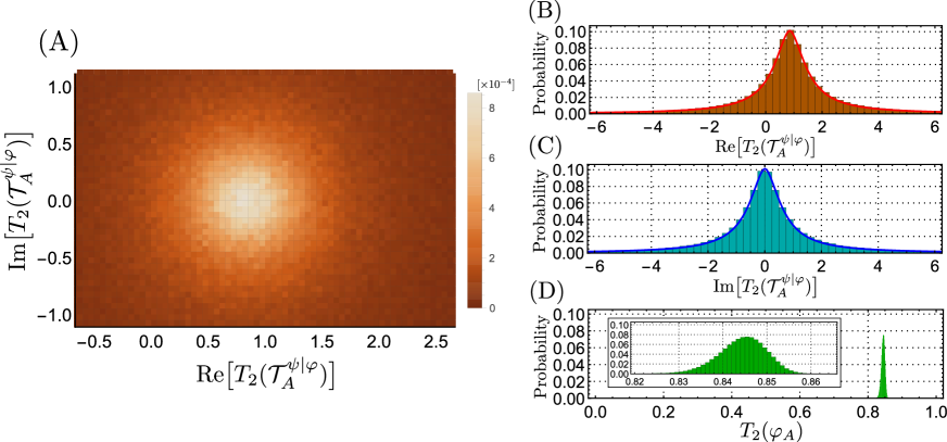
Refer to caption
Figure 7: Distributions of the pseudo Tsallis entropy T2(𝒯Aψ|φ)subscript𝑇2subscriptsuperscript𝒯conditional𝜓𝜑𝐴T_{2}(\mathcal{T}^{\psi|{\varphi}}_{A}) over Haar random states |φket𝜑\ket{{\varphi}} and |ψket𝜓\ket{\psi} (Panels A, B, and C) and that of the entanglement Tsallis entropy T2(φA)subscript𝑇2subscript𝜑𝐴T_{2}({\varphi}_{A}) over |φ𝖧similar-toket𝜑𝖧\ket{\varphi}\sim{\sf H} (Panel D). They are obtained for dimA=8dimensionsubscript𝐴8\dim{\mathcal{H}}_{A}=8 and dimB=32dimensionsubscript𝐵32\dim{\mathcal{H}}_{B}=32 with the number of sampling 655360655360655360. Similarly to Fig. 6, the distribution of the pseudo entropy over its real and imaginary parts is given in Panel (A), that only of the real part in Panel (B), that of the imaginary part in Panel (C), and that of the entanglement Tsallis entropy over a Haar random state in Panel (D). In Panels (B) and (C), we also plot inverse-polynomial functions by red and blue colours (see the main text).

To elucidate this point, we numerically demonstrate in figure 7 the distribution of the entanglement Tsallis entropy and that of pseudo Tsallis entropy over Haar random states. We especially consider q=2𝑞2q=2. It is clear that the shapes of the distributions are rather different: for the entanglement Tsallis entropy, the probability density function (PDF) is basically a Gaussian-shape flanked with rapidly decaying functions on its both sides (see Panel (D) and its inset). In contrast, the distribution of the pseudo Tsallis entropy has much heavier tails and resembles the Cauchy–Lorentz distribution rather than a Gaussian distribution (see Panel (B) and (C)). In fact, we numerically confirmed that the PDF p(Re[T2(𝒯Aψ|φ)]=t)𝑝Redelimited-[]subscript𝑇2superscriptsubscript𝒯𝐴conditional𝜓𝜑𝑡p\bigl{(}{\rm Re}[T_{2}({\mathcal{T}}_{A}^{\psi|\varphi})]=t\bigr{)} for the real part of the pseudo Tsallis entropy with q=2𝑞2q=2 to take the value t𝑡t is given by

p(Re[T2(𝒯Aψ|φ)]=t)1(tt0)1.8, where t0:=1dimA+dimBdim+1.formulae-sequenceproportional-to𝑝Redelimited-[]subscript𝑇2superscriptsubscript𝒯𝐴conditional𝜓𝜑𝑡1superscript𝑡subscript𝑡01.8assign where subscript𝑡01dimensionsubscript𝐴dimensionsubscript𝐵dimension1p\bigl{(}{\rm Re}[T_{2}({\mathcal{T}}_{A}^{\psi|\varphi})]=t\bigr{)}\propto\frac{1}{(t-t_{0})^{1.8}},\text{\ \ where\ \ }t_{0}:=1-\frac{\dim{\mathcal{H}}_{A}+\dim{\mathcal{H}}_{B}}{\dim{\mathcal{H}}+1}. (3.78)

We here point out that this PDF of the pseudo Tsallis entropy shall indicate that the values should be centered around its average t0(0,1)subscript𝑡001t_{0}\in(0,1), suggesting a weak concentration of the pseudo Tsallis entropy for random states. We hence expect that, in the large dimension limit, it is atypical for the pseudo Tsallis entropy to take abnormal values such as complex numbers with large absolute values.

We finally conclude this section with a comment on a theoretically interesting property of the entanglement distribution over a random state. It is known that the PDF for the entanglement entropy over a Haar random state has two singularities, which divides the distribution into three entanglement phases with different entanglement spectra [41, 42, 43, 44, 45, 46, 47, 48]. It is natural to ask whether the PDF p(Re[T2(𝒯Aψ|φ)]=t)𝑝Redelimited-[]subscript𝑇2superscriptsubscript𝒯𝐴conditional𝜓𝜑𝑡p\bigl{(}{\rm Re}[T_{2}({\mathcal{T}}_{A}^{\psi|\varphi})]=t\bigr{)} for the pseudo Tsallis entropy also has any singularity. This question can be analytically addressed using the technique of random matrix theory, which is the method used to analyze the PDF for the entanglement Tsallis entropy in great detail, but we will leave it as an open problem.

4 Pseudo Rényi Entropy in Free CFT

In this section, we compute pseudo Rényi entropy for a free CFT as a simple example of QFT. We consider a massless scalar field theory in two dimensional Euclidean space, whose coordinate is w=x+iτ𝑤𝑥𝑖𝜏w=x+i\tau. We would like to calculate its pseudo-Rényi entropy with respect to an interval subsystem A={(x,τ)τ=0,xlxxr}𝐴conditional-set𝑥𝜏formulae-sequence𝜏0subscript𝑥𝑙𝑥subscript𝑥𝑟A=\{(x,\tau)\mid\tau=0,\ x_{l}\leq x\leq x_{r}\} by using the replica method we described in section 2.4.

Before computing the pseudo Rényi entropy, let us briefly review the ordinary calculation of Rényi entropy of the vacuum state |0ket0\ket{0}, the detail of which is described in [9]. We define the density matrix ρA(0)=TrB[|00|]superscriptsubscript𝜌𝐴0subscriptTr𝐵delimited-[]ket0bra0\rho_{A}^{(0)}=\mathrm{Tr}_{B}[|0\rangle\langle 0|], where B𝐵B is the complement of A𝐴A. In terms of the path integral as expressed in section 2.4, |0ket0\ket{0} and 0|bra0\bra{0} are

|0=[Uncaptioned image],0|=[Uncaptioned image],formulae-sequenceket0[Uncaptioned image]bra0[Uncaptioned image]\displaystyle\ket{0}=\vbox{\hbox{\includegraphics[height=86.11084pt]{FREECFT1.pdf}}},\ \bra{0}=\vbox{\hbox{\includegraphics[height=86.11084pt]{FREECFT2.pdf}}}, (4.1)

and tracing out on B𝐵B then

ρA(0)=[Uncaptioned image].superscriptsubscript𝜌𝐴0[Uncaptioned image]\displaystyle\rho_{A}^{(0)}=\vbox{\hbox{\includegraphics[height=86.11084pt]{FREECFT3.pdf}}}. (4.2)

For calculating the Rényi entropy, we need Tr[(ρA)n]Trdelimited-[]superscriptsubscript𝜌𝐴𝑛\mathrm{Tr}[(\rho_{A})^{n}], which can be computed by replica method. We consider n𝑛n sheets and identify the upper side of A𝐴A on the k𝑘k-th sheet and the lower side of A𝐴A on the (k+1)𝑘1(k+1)-th sheet, that is,

Tr[(ρA(0))n]=[Uncaptioned image].Trdelimited-[]superscriptsuperscriptsubscript𝜌𝐴0𝑛[Uncaptioned image]\displaystyle\mathrm{Tr}[(\rho_{A}^{(0)})^{n}]=\vbox{\hbox{\includegraphics[height=86.11084pt]{FREECFT4}}}. (4.3)

The right-hand side of (4.3) is the path integral on the manifold ΣnsubscriptΣ𝑛\Sigma_{n} introduced in section 2.4. The identification between the k𝑘k-th sheet and the (k+1)𝑘1(k+1)-th sheet corresponds to the multiplication as matrix, especially the (n+1)𝑛1(n+1)-th sheet and the first sheet to tracing out. By computing this path integral, the explicit expression of (4.3) becomes

Tr[(ρA(0))n]=cn(xrxlϵ)n216n,Trdelimited-[]superscriptsuperscriptsubscript𝜌𝐴0𝑛subscript𝑐𝑛superscriptsubscript𝑥𝑟subscript𝑥𝑙italic-ϵsuperscript𝑛216𝑛\mathrm{Tr}[(\rho_{A}^{(0)})^{n}]=c_{n}\left(\frac{x_{r}-x_{l}}{\epsilon}\right)^{-\frac{n^{2}-1}{6n}}, (4.4)

where ϵitalic-ϵ\epsilon is the cutoff with the dimension of length and now the central charge is 111. Also note that cnsubscript𝑐𝑛c_{n} is a constant which depends on n𝑛n and cannnot be determined by the replica trick. Thus the n𝑛n-th Rényi entropy is

S(n)(ρA(0))=16(1+1n)logxrxlϵ+logcn1n.superscript𝑆𝑛superscriptsubscript𝜌𝐴01611𝑛subscript𝑥𝑟subscript𝑥𝑙italic-ϵsubscript𝑐𝑛1𝑛S^{(n)}(\rho_{A}^{(0)})=\frac{1}{6}\left(1+\frac{1}{n}\right)\log\frac{x_{r}-x_{l}}{\epsilon}+\frac{\log{c_{n}}}{1-n}. (4.5)

It is important that the vacuum state has the entanglement between A𝐴A and B𝐵B, so we are interested in the variation of the pseudo Rényi entropy from the ordinary Rényi entropy of the vacuum state:

ΔSA(n)S(n)(𝒯Aψ|φ)S(n)(ρA(0)).Δsubscriptsuperscript𝑆𝑛𝐴superscript𝑆𝑛subscriptsuperscript𝒯conditional𝜓𝜑𝐴superscript𝑆𝑛subscriptsuperscript𝜌0𝐴\Delta S^{(n)}_{A}\equiv S^{(n)}(\mathcal{T}^{\psi|{\varphi}}_{A})-S^{(n)}(\rho^{(0)}_{A}). (4.6)

We will compute this quantity in the following sections.

4.1 Example 1: Exciting the Same Space Point with Different Cutoffs

For the first example, we choose |ψket𝜓\ket{\psi} and |φket𝜑\ket{{\varphi}} as

|ψ=eaHCFT𝒪(x=b)|0,ket𝜓superscript𝑒𝑎subscript𝐻CFT𝒪𝑥𝑏ket0\displaystyle\ket{\psi}=e^{-aH_{\rm CFT}}\mathcal{O}(x=b)\ket{0},
|φ=eaHCFT𝒪(x=b)|0,ket𝜑superscript𝑒superscript𝑎subscript𝐻CFT𝒪𝑥superscript𝑏ket0\displaystyle\ket{{\varphi}}=e^{-a^{\prime}H_{\rm CFT}}\mathcal{O}(x=b^{\prime})\ket{0}, (4.7)

where b𝑏b (bsuperscript𝑏b^{\prime}) is the excited space point and a𝑎a (asuperscript𝑎a^{\prime}) is a cutoff to avoid UV divergence at b=b𝑏superscript𝑏b=b^{\prime}. We can also regard a𝑎a (asuperscript𝑎a^{\prime}) as Euclidean inserting time. The inserted operator is given by

𝒪=ei2ϕ+ei2ϕ,𝒪superscript𝑒𝑖2italic-ϕsuperscript𝑒𝑖2italic-ϕ\mathcal{O}=e^{\frac{i}{2}\phi}+e^{-\frac{i}{2}\phi}, (4.8)

and its conformal dimension is h=h¯=1/8¯18h=\bar{h}=1/8. This operator is analogous to a Bell pair in a two qubit system. Note that this operator creates a Bell pair at the inserted point [27, 28]. This can be seen if we decompose the scalar field into the left moving mode and right moving one as ϕ=ϕR+ϕLitalic-ϕsubscriptitalic-ϕ𝑅subscriptitalic-ϕ𝐿\phi=\phi_{R}+\phi_{L}. We can interpret the operator such that e±iϕL/2|0L|±Lsimilar-tosuperscript𝑒plus-or-minus𝑖subscriptitalic-ϕ𝐿2subscriptket0𝐿subscriptketplus-or-minus𝐿e^{\pm i\phi_{L}/2}|0\rangle_{L}\sim|\pm\rangle_{L} and e±iϕR/2|0R|±Rsimilar-tosuperscript𝑒plus-or-minus𝑖subscriptitalic-ϕ𝑅2subscriptket0𝑅subscriptketplus-or-minus𝑅e^{\pm i\phi_{R}/2}|0\rangle_{R}\sim|\pm\rangle_{R}. This allows us to regard (ei2ϕ+ei2ϕ)|0L|0R|+L|+R+|L|Rsimilar-tosuperscript𝑒𝑖2italic-ϕsuperscript𝑒𝑖2italic-ϕsubscriptket0𝐿subscriptket0𝑅subscriptket𝐿subscriptket𝑅subscriptket𝐿subscriptket𝑅(e^{\frac{i}{2}\phi}+e^{-\frac{i}{2}\phi})|0\rangle_{L}|0\rangle_{R}\sim|+\rangle_{L}|+\rangle_{R}+|-\rangle_{L}|-\rangle_{R}, i.e. a Bell pair. If we chose 𝒪=ei2ϕ𝒪superscript𝑒𝑖2italic-ϕ\mathcal{O}=e^{\frac{i}{2}\phi} instead of (4.8), we would always get the trivial result ΔSA(2)=0Δsubscriptsuperscript𝑆2𝐴0\Delta S^{(2)}_{A}=0.

Note that (4.1) is written in the Schrödinger picture. When we perform the path integral, the corresponding operators are inserted at

(w1,w¯1)(bia,b+ia),(w2,w¯2)(b+ia,bia)formulae-sequencesubscript𝑤1subscript¯𝑤1𝑏𝑖𝑎𝑏𝑖𝑎subscript𝑤2subscript¯𝑤2superscript𝑏𝑖superscript𝑎superscript𝑏𝑖superscript𝑎\displaystyle(w_{1},\bar{w}_{1})\equiv(b-ia,b+ia),\leavevmode\nobreak\ \leavevmode\nobreak\ \leavevmode\nobreak\ \leavevmode\nobreak\ (w_{2},\bar{w}_{2})\equiv(b^{\prime}+ia^{\prime},b^{\prime}-ia^{\prime}) (4.9)

respectively.

Refer to caption
Figure 8: The manifold Σ2subscriptΣ2\Sigma_{2} for the setting in section 4.1. The lower half expresses |ψket𝜓\ket{\psi} and the upper half expresses φ|bra𝜑\bra{{\varphi}}, both of which is excited at the same space point but with different cutoffs. The upper side of the subsystem in the first sheet is identified with the lower side of the subsystem in the second sheet. These correspond to matrix multiplication and tracing out respectively.

Now we consider the case where the same space points are excited with different cutoffs, i.e., we can parameterize as w1=iasubscript𝑤1𝑖𝑎w_{1}=-ia and w2=iasubscript𝑤2𝑖superscript𝑎w_{2}=ia^{\prime}, where a,a>0𝑎superscript𝑎0a,a^{\prime}>0. Let us compute the variation of the second pseudo Rényi entropy ΔSA(2)Δsubscriptsuperscript𝑆2𝐴\Delta S^{(2)}_{A} by replica method as in [27, 28]. The manifold Σ2subscriptΣ2\Sigma_{2} is depicted in figure 8. From the formula (2.37), the pseudo 2nd Rényi entropy is

ΔSA(2)=log(𝒪(w1,w¯1)𝒪(w2,w¯2)𝒪(w3,w¯3)𝒪(w4,w¯4)Σ2(𝒪(w1,w¯1)𝒪(w2,w¯2)Σ1)2).Δsubscriptsuperscript𝑆2𝐴subscriptdelimited-⟨⟩𝒪subscript𝑤1subscript¯𝑤1superscript𝒪subscript𝑤2subscript¯𝑤2𝒪subscript𝑤3subscript¯𝑤3superscript𝒪subscript𝑤4subscript¯𝑤4subscriptΣ2superscriptsubscriptdelimited-⟨⟩𝒪subscript𝑤1subscript¯𝑤1superscript𝒪subscript𝑤2subscript¯𝑤2subscriptΣ12\Delta S^{(2)}_{A}=-\log\left(\frac{\langle\mathcal{O}(w_{1},\bar{w}_{1})\mathcal{O}^{\dagger}(w_{2},\bar{w}_{2})\mathcal{O}(w_{3},\bar{w}_{3})\mathcal{O}^{\dagger}(w_{4},\bar{w}_{4})\rangle_{\Sigma_{2}}}{(\langle\mathcal{O}(w_{1},\bar{w}_{1})\mathcal{O}^{\dagger}(w_{2},\bar{w}_{2})\rangle_{\Sigma_{1}})^{2}}\right). (4.10)

To compute the expectation values in the logarithm, we consider a conformal mapping

wxlwxr=z2.𝑤subscript𝑥𝑙𝑤subscript𝑥𝑟superscript𝑧2\frac{w-x_{l}}{w-x_{r}}=z^{2}. (4.11)

This maps Σ2subscriptΣ2\Sigma_{2} to a Riemann surface Σ1subscriptΣ1\Sigma_{1}. Let ziΣ1(i=1,,4)subscript𝑧𝑖subscriptΣ1𝑖14z_{i}\in\Sigma_{1}\ (i=1,\ldots,4) be points mapped by (4.11) from wiΣ2(i=1,,4)subscript𝑤𝑖subscriptΣ2𝑖14w_{i}\in\Sigma_{2}\ (i=1,\ldots,4) respectively, then there are the relations

z1=z3=w1xlw1xr,subscript𝑧1subscript𝑧3subscript𝑤1subscript𝑥𝑙subscript𝑤1subscript𝑥𝑟\displaystyle z_{1}=-z_{3}=\sqrt{\frac{w_{1}-x_{l}}{w_{1}-x_{r}}}, (4.12)
z2=z4=w2xlw2xr.subscript𝑧2subscript𝑧4subscript𝑤2subscript𝑥𝑙subscript𝑤2subscript𝑥𝑟\displaystyle z_{2}=-z_{4}=\sqrt{\frac{w_{2}-x_{l}}{w_{2}-x_{r}}}. (4.13)

In terms of zisubscript𝑧𝑖z_{i}, ΔSA(2)Δsubscriptsuperscript𝑆2𝐴\Delta S^{(2)}_{A} turns out to be

ΔSA(2)=log(21+|η|+|1η|),Δsubscriptsuperscript𝑆2𝐴21𝜂1𝜂\Delta S^{(2)}_{A}=\log\left(\frac{2}{1+|\eta|+|1-\eta|}\right), (4.14)

where η𝜂\eta is the cross ratio defined as

η=(z1z2)(z3z4)(z1z3)(z2z4).𝜂subscript𝑧1subscript𝑧2subscript𝑧3subscript𝑧4subscript𝑧1subscript𝑧3subscript𝑧2subscript𝑧4\eta=\frac{(z_{1}-z_{2})(z_{3}-z_{4})}{(z_{1}-z_{3})(z_{2}-z_{4})}. (4.15)

When both a𝑎a and asuperscript𝑎a^{\prime} are real (i.e. the Euclidean time evolution), we always find ΔSA(2)0Δsubscriptsuperscript𝑆2𝐴0\Delta S^{(2)}_{A}\leq 0. If we set a=a𝑎superscript𝑎a=a^{\prime}, the pseudo 2nd Rényi entropy reduces to the ordinary 2nd Rényi entropy. Therefore ΔSA(2)=0Δsubscriptsuperscript𝑆2𝐴0\Delta S^{(2)}_{A}=0 when a=a𝑎superscript𝑎a=a^{\prime} [27, 28].

Let us investigate the behavior of ΔSA(2)Δsubscriptsuperscript𝑆2𝐴\Delta S^{(2)}_{A} in an explicit example. Figure 9 shows ΔSA(2)Δsubscriptsuperscript𝑆2𝐴\Delta S^{(2)}_{A} for subsystems centered at different points x=xm(xl+xr2)𝑥annotatedsubscript𝑥𝑚absentsubscript𝑥𝑙subscript𝑥𝑟2x=x_{m}(\equiv\frac{x_{l}+x_{r}}{2}) with length l=20𝑙20l=20, where lxrxl𝑙subscript𝑥𝑟subscript𝑥𝑙l\equiv x_{r}-x_{l}. We can see that ΔSA(2)Δsubscriptsuperscript𝑆2𝐴\Delta S^{(2)}_{A} sharply decreases when either of the operator insertion points become closer to the boundary of the interval A𝐴A. This behavior can be understood from the fact that the pseudo entropy is reduced when we consider the entanglement swapping as we saw in section 3.2.2. Indeed, when the boundary of A𝐴A gets close to one of the operators, the system experiences an entanglement swapping. On the other hand, if we insert an operator in the middle of the interval A𝐴A, since the swapping does not occur near the boundaries of A𝐴A, this does not contribute to ΔSA(2)Δsubscriptsuperscript𝑆2𝐴\Delta S^{(2)}_{A}.

Refer to caption
Figure 9: ΔSA(2)Δsubscriptsuperscript𝑆2𝐴\Delta S^{(2)}_{A} for subsystems centered at different space points with length l=20𝑙20l=20. Blue line: a=4,a=6formulae-sequence𝑎4superscript𝑎6a=4,a^{\prime}=6, orange line: a=2,a=8formulae-sequence𝑎2superscript𝑎8a=2,a^{\prime}=8, green line: a=0.1,a=9.9formulae-sequence𝑎0.1superscript𝑎9.9a=0.1,a^{\prime}=9.9 case.

We can also analyze the real time evolution by setting the Euclidean times as a=δ+it1𝑎𝛿𝑖subscript𝑡1a=\delta+it_{1} and a=δit2superscript𝑎𝛿𝑖subscript𝑡2a^{\prime}=\delta-it_{2}, where δ(>0)annotated𝛿absent0\delta(>0) is an infinitesimally small parameter which regularize the local quench. When 0<xl<t1,2<xr0subscript𝑥𝑙subscript𝑡12subscript𝑥𝑟0<x_{l}<t_{1,2}<x_{r}, we find ΔSA(2)=log2Δsubscriptsuperscript𝑆2𝐴2\Delta S^{(2)}_{A}=\log 2, which is interpreted as the entanglement entropy for the Bell pair as in [27, 28].

4.2 Example 2: Exciting Different Points with the Same Cutoff
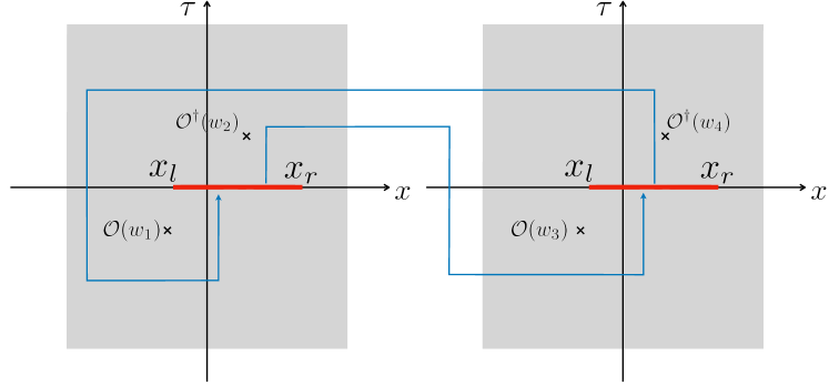
Refer to caption
Figure 10: The manifold Σ2subscriptΣ2\Sigma_{2} for the setting in section 4.2.

We consider the same states as (4.1) and this time we excite two different space points with different cutoffs, i.e. w1=diasubscript𝑤1𝑑𝑖𝑎w_{1}=-d-ia, w2=d+iasubscript𝑤2𝑑𝑖𝑎w_{2}=d+ia as depicted in figure 10. Since the difference from the previous case is only the location of the excitations, ΔSA(2)Δsubscriptsuperscript𝑆2𝐴\Delta S^{(2)}_{A} is the same as (4.14).

Figure 11 shows the behavior of ΔSA(2)Δsubscriptsuperscript𝑆2𝐴\Delta S^{(2)}_{A} as a function of the center of subsystems xmsubscript𝑥𝑚x_{m}. We again see that ΔS(2)Δsuperscript𝑆2\Delta S^{(2)} sharply decreases when an end point of the interval A𝐴A is close to either of the two operator insertion points, which can be interpreted as in the previous example.
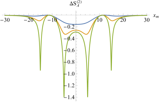
Refer to caption
Figure 11: ΔSA(2)Δsubscriptsuperscript𝑆2𝐴\Delta S^{(2)}_{A} for subsystems centered at different points with length l=20𝑙20l=20. We set the points of excitation at d=5𝑑5d=5. Blue line: a=5𝑎5a=5, orange line: a=2𝑎2a=2, green line: a=0.1𝑎0.1a=0.1 case.

4.3 Example 3: Excitations by Different Operators

In this section, we would like to consider an example of excitations at the same space points by different operators, which is similar to the setup in figure 8. We set w1=iasubscript𝑤1𝑖𝑎w_{1}=-ia and w2=iasubscript𝑤2𝑖superscript𝑎w_{2}=ia^{\prime}, and let two states be

|ψ=eaHCFT𝒪~(x=0)|0,ket𝜓superscript𝑒𝑎subscript𝐻CFT~𝒪𝑥0ket0\displaystyle\ket{\psi}=e^{-aH_{\rm CFT}}\tilde{\mathcal{O}}(x=0)\ket{0},
|φ=eaHCFT𝒪(x=0)|0,ket𝜑superscript𝑒superscript𝑎subscript𝐻CFT𝒪𝑥0ket0\displaystyle\ket{{\varphi}}=e^{-a^{\prime}H_{\rm CFT}}\mathcal{O}(x=0)\ket{0}, (4.16)

where 𝒪𝒪\mathcal{O} is same as defined in (4.8) and 𝒪~~𝒪\tilde{\mathcal{O}} is defined as

𝒪~=ei2ϕ+eiθei2ϕ.~𝒪superscript𝑒𝑖2italic-ϕsuperscript𝑒𝑖𝜃superscript𝑒𝑖2italic-ϕ\displaystyle\tilde{\mathcal{O}}=e^{\frac{i}{2}\phi}+e^{i\theta}e^{-\frac{i}{2}\phi}. (4.17)

Its conformal dimension is also h=h¯=1/8¯18h=\bar{h}=1/8 and θ[π,π]𝜃𝜋𝜋\theta\in[-\pi,\pi]. This is analogous to the states in (3.14). ΔSA(2)Δsubscriptsuperscript𝑆2𝐴\Delta S^{(2)}_{A} can be computed by replica method again, we have

ΔSA(2)=log(𝒪~(w1,w¯1)𝒪(w2,w¯2)𝒪~(w3,w¯3)𝒪(w4,w¯4)Σ2(𝒪~(w1,w¯1)𝒪(w2,w¯2)Σ1)2).Δsubscriptsuperscript𝑆2𝐴subscriptdelimited-⟨⟩~𝒪subscript𝑤1subscript¯𝑤1superscript𝒪subscript𝑤2subscript¯𝑤2~𝒪subscript𝑤3subscript¯𝑤3superscript𝒪subscript𝑤4subscript¯𝑤4subscriptΣ2superscriptsubscriptdelimited-⟨⟩~𝒪subscript𝑤1subscript¯𝑤1superscript𝒪subscript𝑤2subscript¯𝑤2subscriptΣ12\Delta S^{(2)}_{A}=-\log\left(\frac{\langle\tilde{\mathcal{O}}(w_{1},\bar{w}_{1})\mathcal{O}^{\dagger}(w_{2},\bar{w}_{2})\tilde{\mathcal{O}}(w_{3},\bar{w}_{3})\mathcal{O}^{\dagger}(w_{4},\bar{w}_{4})\rangle_{\Sigma_{2}}}{(\langle\tilde{\mathcal{O}}(w_{1},\bar{w}_{1})\mathcal{O}^{\dagger}(w_{2},\bar{w}_{2})\rangle_{\Sigma_{1}})^{2}}\right). (4.18)

Computing the expectation values in the logarithm by using the conformal mapping (4.11),

ΔSA(2)=log(1+cosθcosθ+|η|+|1η|),Δsubscriptsuperscript𝑆2𝐴1𝜃𝜃𝜂1𝜂\Delta S^{(2)}_{A}=\log\left(\frac{1+\cos\theta}{\cos\theta+|\eta|+|1-\eta|}\right), (4.19)

which reduces to (4.14) when θ=0𝜃0\theta=0. From (4.19), ΔSA(2)Δsubscriptsuperscript𝑆2𝐴\Delta S^{(2)}_{A} is always negative.

Refer to caption
Refer to caption
Figure 12: The left figure shows the behavior of ΔSA(2)Δsubscriptsuperscript𝑆2𝐴\Delta S^{(2)}_{A} as functions of the center of the interval A𝐴A i.e. xmsubscript𝑥𝑚x_{m}. Here, we take the length of the subsystem to be l=20𝑙20l=20. We fix the points of excitations at a=3,a=5formulae-sequence𝑎3superscript𝑎5a=3,a^{\prime}=5. Blue line: θ=0𝜃0\theta=0, orange line: θ=π/3𝜃𝜋3\theta=\pi/3, green line: θ=π/2𝜃𝜋2\theta=\pi/2 case. The right figure shows the behavior of ΔSA(2)Δsubscriptsuperscript𝑆2𝐴\Delta S^{(2)}_{A} as a function of the phase θ𝜃\theta at xm=10subscript𝑥𝑚10x_{m}=10 and l=20𝑙20l=20. We also fix the points of excitations at a=3,a=5formulae-sequence𝑎3superscript𝑎5a=3,a^{\prime}=5. ΔSA(2)Δsubscriptsuperscript𝑆2𝐴\Delta S^{(2)}_{A} diverges at θ=±π𝜃plus-or-minus𝜋\theta=\pm\pi.

Figure 12 shows the behavior of ΔSA(2)Δsubscriptsuperscript𝑆2𝐴\Delta S^{(2)}_{A} when we change the phase θ𝜃\theta of 𝒪~~𝒪\tilde{\mathcal{O}}. The left panel shows ΔSA(2)Δsubscriptsuperscript𝑆2𝐴\Delta S^{(2)}_{A} as functions of the center of subsections xmsubscript𝑥𝑚x_{m} and the right as a function of the phase θ𝜃\theta. We can see that ΔSA(2)Δsubscriptsuperscript𝑆2𝐴\Delta S^{(2)}_{A} becomes smaller when the “difference” between 𝒪𝒪\mathcal{O} and 𝒪~~𝒪\tilde{\mathcal{O}} is larger.

In the Lorentzian time evolution, we set a=δ+it𝑎𝛿𝑖𝑡a=\delta+it and a=δitsuperscript𝑎𝛿𝑖𝑡a^{\prime}=\delta-it. If we take the limit δ0𝛿0\delta\to 0 and assume the range 0<xl<t<xr0subscript𝑥𝑙𝑡subscript𝑥𝑟0<x_{l}<t<x_{r}, which is equivalent to the limit (η,η¯)(1,0)𝜂¯𝜂10(\eta,\bar{\eta})\to(1,0), we obtain

ΔSA(2)=log(1+cosθcosθ).Δsubscriptsuperscript𝑆2𝐴1𝜃𝜃\Delta S^{(2)}_{A}=\log\left(\frac{1+\cos\theta}{\cos\theta}\right). (4.20)

This agrees with the previous result (3.17) of a two qubit system as expected.

Moreover, we can compute the pseudo 3rd Rényi entropy by replica method. In this case, we consider the manifold Σ3subscriptΣ3\Sigma_{3} composed by three sheets. Then we have

ΔSA(3)=12log(𝒪~(w1,w¯1)𝒪(w2,w¯2)𝒪~(w3,w¯3)𝒪(w4,w¯4)𝒪~(w5,w¯5)𝒪(w6,w¯6)Σ3(𝒪~(w1,w¯1)𝒪(w2,w¯2)Σ1)3).Δsubscriptsuperscript𝑆3𝐴12subscriptdelimited-⟨⟩~𝒪subscript𝑤1subscript¯𝑤1superscript𝒪subscript𝑤2subscript¯𝑤2~𝒪subscript𝑤3subscript¯𝑤3superscript𝒪subscript𝑤4subscript¯𝑤4~𝒪subscript𝑤5subscript¯𝑤5superscript𝒪subscript𝑤6subscript¯𝑤6subscriptΣ3superscriptsubscriptdelimited-⟨⟩~𝒪subscript𝑤1subscript¯𝑤1superscript𝒪subscript𝑤2subscript¯𝑤2subscriptΣ13\Delta S^{(3)}_{A}=-\frac{1}{2}\log\left(\frac{\langle\tilde{\mathcal{O}}(w_{1},\bar{w}_{1})\mathcal{O}^{\dagger}(w_{2},\bar{w}_{2})\tilde{\mathcal{O}}(w_{3},\bar{w}_{3})\mathcal{O}^{\dagger}(w_{4},\bar{w}_{4})\tilde{\mathcal{O}}(w_{5},\bar{w}_{5})\mathcal{O}^{\dagger}(w_{6},\bar{w}_{6})\rangle_{\Sigma_{3}}}{(\langle\tilde{\mathcal{O}}(w_{1},\bar{w}_{1})\mathcal{O}^{\dagger}(w_{2},\bar{w}_{2})\rangle_{\Sigma_{1}})^{3}}\right). (4.21)

The expectation values are computed in a Riemann surface mapped by conformal mapping

wxlwxr=z3,𝑤subscript𝑥𝑙𝑤subscript𝑥𝑟superscript𝑧3\displaystyle\frac{w-x_{l}}{w-x_{r}}=z^{3}, (4.22)

then the new coordinates have the following relations:

z1subscript𝑧1\displaystyle z_{1} =e23πiz3=e23πiz5=(w1xlw1xr)1/3,absentsuperscript𝑒23𝜋𝑖subscript𝑧3superscript𝑒23𝜋𝑖subscript𝑧5superscriptsubscript𝑤1subscript𝑥𝑙subscript𝑤1subscript𝑥𝑟13\displaystyle=e^{-\frac{2}{3}\pi i}z_{3}=e^{\frac{2}{3}\pi i}z_{5}=\left(\frac{w_{1}-x_{l}}{w_{1}-x_{r}}\right)^{1/3}, (4.23)
z2subscript𝑧2\displaystyle z_{2} =e23πiz4=e23πiz6=(w2xlw2xr)1/3.absentsuperscript𝑒23𝜋𝑖subscript𝑧4superscript𝑒23𝜋𝑖subscript𝑧6superscriptsubscript𝑤2subscript𝑥𝑙subscript𝑤2subscript𝑥𝑟13\displaystyle=e^{-\frac{2}{3}\pi i}z_{4}=e^{\frac{2}{3}\pi i}z_{6}=\left(\frac{w_{2}-x_{l}}{w_{2}-x_{r}}\right)^{1/3}. (4.24)

We define cross ratios

ηijkl=(zizj)(zkzl)(zizk)(zjzl),superscriptsubscript𝜂𝑖𝑗𝑘𝑙subscript𝑧𝑖subscript𝑧𝑗subscript𝑧𝑘subscript𝑧𝑙subscript𝑧𝑖subscript𝑧𝑘subscript𝑧𝑗subscript𝑧𝑙\eta_{ij}^{kl}=\frac{(z_{i}-z_{j})(z_{k}-z_{l})}{(z_{i}-z_{k})(z_{j}-z_{l})}, (4.25)

where the subscripts and superscripts are 1i,j,k,l6formulae-sequence1𝑖𝑗𝑘𝑙61\leq i,j,k,l\leq 6. In terms of ηijklsuperscriptsubscript𝜂𝑖𝑗𝑘𝑙\eta_{ij}^{kl}, ΔSA(3)Δsubscriptsuperscript𝑆3𝐴\Delta S^{(3)}_{A} can be computed as

ΔSA(3)=12log(2(1+cosθ)32cos32θ+3cosθ2(|η1432|2+|η5614|2+|η3256|2)).Δsubscriptsuperscript𝑆3𝐴122superscript1𝜃3232𝜃3𝜃2superscriptsuperscriptsubscript𝜂14322superscriptsuperscriptsubscript𝜂56142superscriptsuperscriptsubscript𝜂32562\Delta S^{(3)}_{A}=\frac{1}{2}\log\left(\frac{\sqrt{2}(1+\cos\theta)^{\frac{3}{2}}}{\cos\frac{3}{2}\theta+3\cos\frac{\theta}{2}(|\eta_{14}^{32}|^{2}+|\eta_{56}^{14}|^{2}+|\eta_{32}^{56}|^{2})}\right). (4.26)
Refer to caption
Refer to caption
Figure 13: The left figure shows the behavior of ΔSA(3)Δsubscriptsuperscript𝑆3𝐴\Delta S^{(3)}_{A} as functions of the center of the interval A𝐴A i.e. xmsubscript𝑥𝑚x_{m}. Here, we take the length of the subsystem to be l=20𝑙20l=20. We fix the points of excitations at a=3,a=5formulae-sequence𝑎3superscript𝑎5a=3,a^{\prime}=5. Blue line: θ=0𝜃0\theta=0, orange line: θ=π/3𝜃𝜋3\theta=\pi/3, green line: θ=π/2𝜃𝜋2\theta=\pi/2 case. The right figure shows the behavior of ΔSA(3)Δsubscriptsuperscript𝑆3𝐴\Delta S^{(3)}_{A} as a function of the phase θ𝜃\theta at xm=10subscript𝑥𝑚10x_{m}=10 and l=20𝑙20l=20. We also fix the points of excitations at a=3,a=5formulae-sequence𝑎3superscript𝑎5a=3,a^{\prime}=5. ΔSA(3)Δsubscriptsuperscript𝑆3𝐴\Delta S^{(3)}_{A} diverges at θ=±π𝜃plus-or-minus𝜋\theta=\pm\pi.

The behavior of ΔSA(3)Δsubscriptsuperscript𝑆3𝐴\Delta S^{(3)}_{A} is similar to that of ΔSA(2)Δsubscriptsuperscript𝑆2𝐴\Delta S^{(2)}_{A}. Figure 13 shows the behavior of ΔSA(3)Δsubscriptsuperscript𝑆3𝐴\Delta S^{(3)}_{A}, which are very similar to the graphs in figure 12.

In the Lorenzian time evolution 0<xl<t<xr0subscript𝑥𝑙𝑡subscript𝑥𝑟0<x_{l}<t<x_{r} with the limit δ0𝛿0\delta\to 0, we find

ΔSA(3)=12log(2(1+cosθ)32cos32θ),Δsubscriptsuperscript𝑆3𝐴122superscript1𝜃3232𝜃\Delta S^{(3)}_{A}=\frac{1}{2}\log\left(\frac{\sqrt{2}(1+\cos\theta)^{\frac{3}{2}}}{\cos{\frac{3}{2}\theta}}\right), (4.27)

which again reproduces the two qubit result (3.16) at n=3𝑛3n=3.

5 Aspects of Holographic Pseudo Entropy

In this section we will explore properties of holographic pseudo entropy defined by the minimal area formula (2.40) from various viewpoints including explicit examples.

5.1 Nonnegativeness of Holographic Pseudo (Rényi) Entropy

One surprising prediction of the holographic pseudo entropy is that this quantity is real and non-negative in the classical gravity dual calculation when we assume the bulk metric is real valued, in spite of the fact that the pseudo entropy S(𝒯Aψ|φ)𝑆subscriptsuperscript𝒯conditional𝜓𝜑𝐴S({\mathcal{T}}^{\psi|{\varphi}}_{A}) takes complex values for generic choices of |ψket𝜓|\psi\rangle and |φket𝜑|{\varphi}\rangle. Moreover, a further holographic consideration shows that pseudo (Rényi) entropies are also real and non-negative in holographic computations:

n>0,S(n)(𝒯Aψ|φ)0.formulae-sequencesuperscript𝑛for-all0superscript𝑆𝑛subscriptsuperscript𝒯conditional𝜓𝜑𝐴0\leavevmode\nobreak\ {}^{\forall}n>0,\leavevmode\nobreak\ S^{(n)}({\mathcal{T}}^{\psi|{\varphi}}_{A})\geq 0. (5.1)

To see this, similar to [49], we compute a refined version of the pseudo Rényi entropy holographically as

S~(n)(𝒯Aψ|φ)n2n(n1nS(n)(𝒯Aψ|φ))=minΓA(n)(AreaofΓA(n)4GN),superscript~𝑆𝑛subscriptsuperscript𝒯conditional𝜓𝜑𝐴superscript𝑛2𝑛𝑛1𝑛superscript𝑆𝑛subscriptsuperscript𝒯conditional𝜓𝜑𝐴subscriptsuperscriptsubscriptΓ𝐴𝑛AreaofsubscriptsuperscriptΓ𝑛𝐴4subscript𝐺𝑁\displaystyle\tilde{S}^{(n)}({\mathcal{T}}^{\psi|{\varphi}}_{A})\equiv n^{2}\frac{\partial}{\partial n}\left(\frac{n-1}{n}S^{(n)}({\mathcal{T}}^{\psi|{\varphi}}_{A})\right)=\min_{\Gamma_{A}^{(n)}}\left(\frac{{\rm Area\leavevmode\nobreak\ of\leavevmode\nobreak\ }\Gamma^{(n)}_{A}}{4G_{N}}\right), (5.2)

where ΓA(n)subscriptsuperscriptΓ𝑛𝐴\Gamma^{(n)}_{A} is a codimension-2 cosmic brane with tension

Tn=14GNn1n.subscript𝑇𝑛14subscript𝐺𝑁𝑛1𝑛\displaystyle T_{n}=\frac{1}{4G_{N}}\frac{n-1}{n}. (5.3)

and satisfies ΓA(n)=AsuperscriptsubscriptΓ𝐴𝑛𝐴\partial\Gamma_{A}^{(n)}=\partial A. Therefore, S~(n)(𝒯Aψ|φ)superscript~𝑆𝑛subscriptsuperscript𝒯conditional𝜓𝜑𝐴\tilde{S}^{(n)}({\mathcal{T}}^{\psi|{\varphi}}_{A}) is supposed to be nonnegative for any n>0𝑛0n>0. Since the pseudo Rényi entropy is just given by the following integral

S(n)(𝒯Aψ|φ)=nn11n𝑑nS~(n)(𝒯Aψ|φ)n2,superscript𝑆𝑛subscriptsuperscript𝒯conditional𝜓𝜑𝐴𝑛𝑛1superscriptsubscript1𝑛differential-dsuperscript𝑛superscript~𝑆𝑛subscriptsuperscript𝒯conditional𝜓𝜑𝐴superscript𝑛2\displaystyle S^{(n)}({\mathcal{T}}^{\psi|{\varphi}}_{A})=\frac{n}{n-1}\int_{1}^{n}dn^{\prime}\frac{\tilde{S}^{(n)}({\mathcal{T}}^{\psi|{\varphi}}_{A})}{n^{\prime 2}}, (5.4)

the non-negativity (5.1) is shown.

The inequalities (5.1) give strong restrictions in the sense that holographic transition matrices belong to (at least) class \mathscr{B}. This can be regarded as a new characterization of holographic states.

5.2 Subadditivity and Strong Subadditivity

Since the holographic pseudo entropy is real and non-negative, we can think of possibilities of other inequalities. It is clear to confirm the subadditivity expressed as

S(𝒯Aψ|φ)+S(𝒯Bψ|φ)S(𝒯ABψ|φ)0.𝑆subscriptsuperscript𝒯conditional𝜓𝜑𝐴𝑆subscriptsuperscript𝒯conditional𝜓𝜑𝐵𝑆subscriptsuperscript𝒯conditional𝜓𝜑𝐴𝐵0\displaystyle S({\mathcal{T}}^{\psi|{\varphi}}_{A})+S({\mathcal{T}}^{\psi|{\varphi}}_{B})-S({\mathcal{T}}^{\psi|{\varphi}}_{AB})\geq 0. (5.5)

Remember that the subadditivity is not always satisfied even if the eigenvalues of transition matrices are real and non-negative as we saw in section 3.4.

Next, let us turn to the strong subadditivity

S(𝒯ABψ|φ)+S(𝒯BCψ|φ)S(𝒯Bψ|φ)S(𝒯ABCψ|φ)?0superscript?𝑆subscriptsuperscript𝒯conditional𝜓𝜑𝐴𝐵𝑆subscriptsuperscript𝒯conditional𝜓𝜑𝐵𝐶𝑆subscriptsuperscript𝒯conditional𝜓𝜑𝐵𝑆subscriptsuperscript𝒯conditional𝜓𝜑𝐴𝐵𝐶0\displaystyle S({\mathcal{T}}^{\psi|{\varphi}}_{AB})+S({\mathcal{T}}^{\psi|{\varphi}}_{BC})-S({\mathcal{T}}^{\psi|{\varphi}}_{B})-S({\mathcal{T}}^{\psi|{\varphi}}_{ABC})\stackrel{{\scriptstyle?}}{{\geq}}0 (5.6)

In the static background, we can prove the strong subadditivity immediately by restricting to a canonical time slice [50]. In the Lorentzian signature, namely the covariant holographic entanglement entropy [12], we can employ the property that the minimal area on a time slice gets smaller as we deform the time slice away from the one which includes the true extremal surface, even if the all relevant extremal surfaces are not on the same time slice, as proved in [51].

However, in our Euclidean time-dependent setup, if we allow to deform the time slice to an arbitrary shape, which is dual to a quantum state via the Euclidean path-integral in CFT, we will immediately find that the strong subadditivity (5.6) can be violated as follows888We would like to thank very much a referee of this article for pointing out this important fact.. Consider a static AdS3 for simplicity and take a canonical time slice. We define four points (P,Q,R,S)𝑃𝑄𝑅𝑆(P,Q,R,S) which are lining up in this order on the time slice. If we take the subsystems A=[P,Q],B=[Q,R]formulae-sequence𝐴𝑃𝑄𝐵𝑄𝑅A=[P,Q],B=[Q,R] and C=[R,S]𝐶𝑅𝑆C=[R,S], then the strong subadditivity follows based on the argument of [50]. However, if we choose a distorted slice which passes through the points in the order (P,Q,S,R)𝑃𝑄𝑆𝑅(P,Q,S,R), then it is obvious that the strong subadditivity is violated because the strong subadditivity takes the opposite ‘wrong’ form S(𝒯ABψ|φ)+S(𝒯BCψ|φ)S(𝒯Bψ|φ)+S(𝒯ABCψ|φ)𝑆subscriptsuperscript𝒯conditional𝜓𝜑𝐴𝐵𝑆subscriptsuperscript𝒯conditional𝜓𝜑𝐵𝐶𝑆subscriptsuperscript𝒯conditional𝜓𝜑𝐵𝑆subscriptsuperscript𝒯conditional𝜓𝜑𝐴𝐵𝐶S({\mathcal{T}}^{\psi|{\varphi}}_{AB})\!+\!S({\mathcal{T}}^{\psi|{\varphi}}_{BC})\!\leq\!S({\mathcal{T}}^{\psi|{\varphi}}_{B})\!+\!S({\mathcal{T}}^{\psi|{\varphi}}_{ABC}). This problem might suggest that the notion of strong subadditivity is not useful in Euclidean setups.

Nevertheless, thinking of possible inequality analogous to the ordinary strong subadditivity in Lorentzian setups, we may focus on the strong subadditivity of holographic pseudo entropy by restricting the time slice to the canonical one on the AdS boundary, assuming that the AdS boundary is the flat space in this paper. Even under this restricted definition, we cannot derive the strong subadditivity of the holographic pseudo entropy because the minimal area gets larger if we deform the time slice, which prohibits a similar proof [51]. Let us mention, however, that we did not find any violation of (5.6) for explicit examples of classical gravity duals we studied. If we can consider a quantum mechanical superposition of several classical geometries, then as we will show in section 5.6, we will find examples which violate these inequalities as coefficients of linear combinations allow complex numbers.

5.3 A Simple Example: Janus AdS/CFT

As a simple example, we would like to analyze the holography for the Janus solutions which are dual to interface CFTs. We focus on a Janus solution in AdS3/CFT2 found in [52].

5.3.1 Holographic Pseudo Entropy in Janus AdS/CFT

The Janus solution to three dimensional AdS gravity coupled to a scalar field:

I=116πGNd3xg(Raϕaϕ+2),𝐼116𝜋subscript𝐺𝑁superscript𝑑3𝑥𝑔𝑅subscript𝑎italic-ϕsuperscript𝑎italic-ϕ2\displaystyle I=\frac{1}{16\pi G_{N}}\int d^{3}x\sqrt{g}(R-\partial_{a}\phi\partial^{a}\phi+2), (5.7)

is given by

ds2=dρ2+f(ρ)dx2+dy2y2,𝑑superscript𝑠2𝑑superscript𝜌2𝑓𝜌𝑑superscript𝑥2𝑑superscript𝑦2superscript𝑦2\displaystyle ds^{2}=d\rho^{2}+f(\rho)\frac{dx^{2}+dy^{2}}{y^{2}},
ϕ=ϕ0+12log[1+12γ2+2γtanhρ1+12γ22γtanhρ],italic-ϕsubscriptitalic-ϕ012112superscript𝛾22𝛾𝜌112superscript𝛾22𝛾𝜌\displaystyle\phi=\phi_{0}+\frac{1}{\sqrt{2}}\log\left[\frac{1+\sqrt{1-2\gamma^{2}}+\sqrt{2}\gamma\tanh\rho}{1+\sqrt{1-2\gamma^{2}}-\sqrt{2}\gamma\tanh\rho}\right],
f(ρ)=12(1+12γ2cosh2ρ),𝑓𝜌12112superscript𝛾22𝜌\displaystyle f(\rho)=\frac{1}{2}\left(1+\sqrt{1-2\gamma^{2}}\cosh 2\rho\right), (5.8)

where 0ρ0𝜌0\leq\rho\leq\infty. If we set γ=0𝛾0\gamma=0, this solution is equivalent to the ordinary Poincare AdS3 solution ds2=dz2+dτ2+dx2z2𝑑superscript𝑠2𝑑superscript𝑧2𝑑superscript𝜏2𝑑superscript𝑥2superscript𝑧2ds^{2}=\frac{dz^{2}+d\tau^{2}+dx^{2}}{z^{2}}.

If we write the exactly marginal operator (i.e. dimension two primary operator) dual to the bulk massless scalar field ϕitalic-ϕ\phi as O(x)𝑂𝑥O(x), then the above Janus solution is dual to a two dimensional holographic CFT deformed by J+𝑑x2O(x)subscript𝐽differential-dsuperscript𝑥2𝑂𝑥J_{+}\int dx^{2}O(x) in the region τ>0𝜏0\tau>0 and by J𝑑x2O(x)subscript𝐽differential-dsuperscript𝑥2𝑂𝑥J_{-}\int dx^{2}O(x) in the region τ<0𝜏0\tau<0, where J±=limρ±ϕ(ρ)subscript𝐽plus-or-minussubscript𝜌plus-or-minusitalic-ϕ𝜌J_{\pm}=\lim_{\rho\to\pm\infty}\phi(\rho). These two deformations produce different states ψ+|brasubscript𝜓\langle\psi_{+}| and |ψketsubscript𝜓|\psi_{-}\rangle, respectively and the total gravity partition function is equal to the inner product ψ+|ψinner-productsubscript𝜓subscript𝜓\langle\psi_{+}|\psi_{-}\rangle.

The time slice τ=0𝜏0\tau=0 is equivalent to ρ=0𝜌0\rho=0 in (5.8). By requiring the usual UV cutoff condition gxx=1ϵ2subscript𝑔𝑥𝑥1superscriptitalic-ϵ2g_{xx}=\frac{1}{\epsilon^{2}} we find the cutoff of the y𝑦y coordinate : y>δ𝑦𝛿y>\delta is given by

δ=ϵf(0)=1+12γ22ϵ.𝛿italic-ϵ𝑓0112superscript𝛾22italic-ϵ\displaystyle\delta=\epsilon\cdot\sqrt{f(0)}=\sqrt{\frac{1+\sqrt{1-2\gamma^{2}}}{2}}\cdot\epsilon. (5.9)

When A𝐴A is a length l𝑙l interval, the holographic pseudo entropy is calculated as the length of geodesic and this leads to

S(𝒯Aψ|ψ+)=c31+12γ22loglδc3(1γ24)loglϵ+c12γ2.𝑆subscriptsuperscript𝒯conditionalsubscript𝜓subscript𝜓𝐴𝑐3112superscript𝛾22𝑙𝛿similar-to-or-equals𝑐31superscript𝛾24𝑙italic-ϵ𝑐12superscript𝛾2\displaystyle S({\mathcal{T}}^{\psi_{-}|\psi_{+}}_{A})=\frac{c}{3}\cdot\sqrt{\frac{1+\sqrt{1-2\gamma^{2}}}{2}}\cdot\log\frac{l}{\delta}\simeq\frac{c}{3}\left(1-\frac{\gamma^{2}}{4}\right)\log\frac{l}{\epsilon}+\frac{c}{12}\gamma^{2}. (5.10)

Therefore we find the holographic pseudo entropy is reduced by O(γ2)𝑂superscript𝛾2O(\gamma^{2}) compared with the γ=0𝛾0\gamma=0 result (i.e. the vacuum case |ψ+=|ψ=|0ketsubscript𝜓ketsubscript𝜓ket0|\psi_{+}\rangle=|\psi_{-}\rangle=|0\rangle) due to the interface perturbation. This result is consistent with the perturbative analysis in (E.21).

5.3.2 CFT Perturbation Analysis

Let us analyze the previous Janus setup from the CFT viewpoint. In the replica calculation of pseudo entropy (look at figure 2), we write the exactly marginal perturbation from ϕ=ϕitalic-ϕsubscriptitalic-ϕ\phi=\phi_{-} to ϕ=ϕ+italic-ϕsubscriptitalic-ϕ\phi=\phi_{+} as Σn(+)𝑑x2JO(x)subscriptsubscriptΣ𝑛differential-dsuperscript𝑥2𝐽𝑂𝑥\int_{\Sigma_{n(+)}}dx^{2}JO(x), where J=J+J𝐽subscript𝐽subscript𝐽J=J_{+}-J_{-} and ΣnsubscriptΣ𝑛\Sigma_{n} is the nlimit-from𝑛n-sheeted Riemann surface. Also we call the upper half of ΣnsubscriptΣ𝑛\Sigma_{n} as Σn(+)subscriptΣ𝑛\Sigma_{n(+)}. The flat complex plane 2superscript2\mathbb{R}^{2} is denoted by Σ=Σn=1ΣsubscriptΣ𝑛1\Sigma=\Sigma_{n=1}.

In the path-integral, the pseudo entropy is computed via the replica method as follows

SA(n)=11nlog[eΣn(+)𝑑x2JO(x)Σn(eΣ1(+)𝑑x2JO(x)Σ1)n].subscriptsuperscript𝑆𝑛𝐴11𝑛subscriptdelimited-⟨⟩superscript𝑒subscriptsubscriptΣ𝑛differential-dsuperscript𝑥2𝐽𝑂𝑥subscriptΣ𝑛superscriptsubscriptdelimited-⟨⟩superscript𝑒subscriptsubscriptΣ1differential-dsuperscript𝑥2𝐽𝑂𝑥subscriptΣ1𝑛\displaystyle S^{(n)}_{A}=\frac{1}{1-n}\log\left[\frac{\langle e^{\int_{\Sigma_{n(+)}}dx^{2}JO(x)}\rangle_{\Sigma_{n}}}{\left(\langle e^{\int_{\Sigma_{1(+)}}dx^{2}JO(x)}\rangle_{\Sigma_{1}}\right)^{n}}\right]. (5.11)

If we take the difference from the entanglement entropy of ϕ=ϕitalic-ϕsubscriptitalic-ϕ\phi=\phi_{-} theory and perform the perturbation w.r.t J𝐽J up to the quadratic order, we get

ΔSA(n)=J21n[𝑑x2𝑑y2O(x)O(y)Σnn𝑑x2𝑑y2O(x)O(y)Σ1].Δsubscriptsuperscript𝑆𝑛𝐴superscript𝐽21𝑛delimited-[]differential-dsuperscript𝑥2differential-dsuperscript𝑦2subscriptdelimited-⟨⟩𝑂𝑥𝑂𝑦subscriptΣ𝑛𝑛differential-dsuperscript𝑥2differential-dsuperscript𝑦2subscriptdelimited-⟨⟩𝑂𝑥𝑂𝑦subscriptΣ1\displaystyle\Delta S^{(n)}_{A}=\frac{J^{2}}{1-n}\left[\int dx^{2}\int dy^{2}\langle O(x)O(y)\rangle_{\Sigma_{n}}-n\int dx^{2}\int dy^{2}\langle O(x)O(y)\rangle_{\Sigma_{1}}\right]. (5.12)

The part []delimited-[][\cdot\cdot\cdot] is estimated as (we introduce the point splitting cut off ϵitalic-ϵ\epsilon)

[]=a1loglϵ+O(1),delimited-[]subscript𝑎1𝑙italic-ϵ𝑂1\displaystyle[\cdot\cdot\cdot]=a_{1}\log\frac{l}{\epsilon}+O(1), (5.13)

where a1>0subscript𝑎10a_{1}>0 are positive constant and also a1n1proportional-tosubscript𝑎1𝑛1a_{1}\propto n-1 as these divergences arise when both x𝑥x and y𝑦y are close to one of two end points of A𝐴A. The divergences arise when the two points x𝑥x and y𝑦y get closer to each other geometrically. Though the integrals of the two point function in (5.12) include O(l2ϵ2)𝑂superscript𝑙2superscriptitalic-ϵ2O(\frac{l^{2}}{\epsilon^{2}}) terms, they cancel with each other as this quadratic divergences are also equally present in the flat space Σ1=2subscriptΣ1superscript2\Sigma_{1}=\mathbb{R}^{2}. We can explicitly confirm that a logarithmic term in (5.13) arises via the non-trivial conformal map (2.38), which vanishes at n=1𝑛1n=1.

Thus we have the estimation (up to an O(1)𝑂1O(1) factor):

ΔSAJ2loglϵ.similar-toΔsubscript𝑆𝐴superscript𝐽2𝑙italic-ϵ\displaystyle\Delta S_{A}\sim-J^{2}\log\frac{l}{\epsilon}. (5.14)

For the Janus setup the scalar action is normalized such that J2cγ2similar-tosuperscript𝐽2𝑐superscript𝛾2J^{2}\sim c\gamma^{2}. Therefore we can reproduce the behavior (5.10).

Note also that the terms (5.11) are in agreement with (E.18) in the general argument of perturbation theory given in appendix E. When two O𝑂Os are on the same sheet of Σ2subscriptΣ2\Sigma_{2}, we have the second term in (E.18), while not on the same sheet, we get the third term in (E.18).

5.4 Pseudo Entropy of Locally Excited States in Holographic CFT

In this subsection we will calculate holographic pseudo entropy for locally excited states [27, 28] in two dimensional CFTs. In AdS/3{}_{3}/CFT2, it is known that the dual geodesic lengths in a gravity dual with local excitations agree with those obtained from the two point functions of light operators in an excited state with heavy operators in holographic CFTs [53]. For example, the holographic entanglement entropy under local quenches [54] can be perfectly reproduced from the CFT calculations [55]. Therefore, below, we will present results of the pseudo entropy computed from a two dimensional holographic CFT. These are guaranteed to agree with those computed from the gravity dual using the formula (2.40) and thus we will omit the gravity dual calculation below. Refer also to appendix F for general analysis of pseudo entropy and fidelity for local operator excited states.

In the former sections, we perform the replica trick, i.e. compute the correlation functions on a replica manifold ΣnsubscriptΣ𝑛\Sigma_{n} to get the pseudo n𝑛n-th Rényi entropy. In CFT2, the replica trick admits a so-called twist operator formalism [56]. In this formalism, instead of computing correlation functions on ΣnsubscriptΣ𝑛\Sigma_{n}, we compute the correlation functions of an n𝑛n replicated CFT with twist operators inserted on the edges of A𝐴A. More specifically, in our case where scalar primaries 𝒪𝒪{\mathcal{O}} with conformal dimension (h𝒪,h𝒪)subscript𝒪subscript𝒪(h_{\mathcal{O}},h_{\mathcal{O}}) are inserted, we can compute the variation of the pseudo n𝑛n-th Rényi entropy from that in the vacuum state by using the twist operator formalism:

ΔSA(n)Δsubscriptsuperscript𝑆𝑛𝐴\displaystyle\Delta S^{(n)}_{A} =S(n)(𝒯Aψ|φ)S(n)(TrAc|00|)absentsuperscript𝑆𝑛subscriptsuperscript𝒯conditional𝜓𝜑𝐴superscript𝑆𝑛subscriptTrsuperscript𝐴𝑐ket0bra0\displaystyle=S^{(n)}({\mathcal{T}}^{\psi|{\varphi}}_{A})-S^{(n)}(\mathrm{Tr}_{A^{c}}|0\rangle\langle 0|)
=11nlog𝒪n(z1,z¯1)σn(z2,z¯2)σ~n(z3,z¯3)𝒪n(z4,z¯4)𝒪n(z1,z¯1)𝒪n(z4,z¯4)σn(z2,z¯2)σ~n(z3,z¯3).absent11𝑛expectationsubscript𝒪𝑛subscript𝑧1subscript¯𝑧1subscript𝜎𝑛subscript𝑧2subscript¯𝑧2subscript~𝜎𝑛subscript𝑧3subscript¯𝑧3subscript𝒪𝑛subscript𝑧4subscript¯𝑧4expectationsubscript𝒪𝑛subscript𝑧1subscript¯𝑧1subscript𝒪𝑛subscript𝑧4subscript¯𝑧4expectationsubscript𝜎𝑛subscript𝑧2subscript¯𝑧2subscript~𝜎𝑛subscript𝑧3subscript¯𝑧3\displaystyle=\frac{1}{1-n}\log\frac{\braket{{\mathcal{O}}_{n}(z_{1},\bar{z}_{1})\sigma_{n}(z_{2},\bar{z}_{2})\tilde{\sigma}_{n}(z_{3},\bar{z}_{3}){\mathcal{O}}_{n}(z_{4},\bar{z}_{4})}}{\braket{{\mathcal{O}}_{n}(z_{1},\bar{z}_{1}){\mathcal{O}}_{n}(z_{4},\bar{z}_{4})}\braket{\sigma_{n}(z_{2},\bar{z}_{2})\tilde{\sigma}_{n}(z_{3},\bar{z}_{3})}}. (5.15)

Here, the correlation functions are those in the n𝑛n replicated CFT whose central charge is nc𝑛𝑐nc, 𝒪n𝒪𝒪𝒪subscript𝒪𝑛tensor-product𝒪𝒪𝒪{\mathcal{O}}_{n}\equiv{\mathcal{O}}\otimes{\mathcal{O}}\otimes\cdots\otimes{\mathcal{O}} is the replicated primary whose conformal weight is (nh𝒪,nh𝒪)𝑛subscript𝒪𝑛subscript𝒪(nh_{\mathcal{O}},nh_{\mathcal{O}}) and σnsubscript𝜎𝑛\sigma_{n}(σ¯nsubscript¯𝜎𝑛\bar{\sigma}_{n}) is the n𝑛n-th twist operator with conformal weight

(hn,h¯n)=(c24(n1n),c24(n1n)).subscript𝑛subscript¯𝑛𝑐24𝑛1𝑛𝑐24𝑛1𝑛\displaystyle(h_{n},\bar{h}_{n})=\left(\frac{c}{24}\left(n-\frac{1}{n}\right),\frac{c}{24}\left(n-\frac{1}{n}\right)\right). (5.16)

If we focus on the pseudo entropy which is given by n1𝑛1n\rightarrow 1 limit, we can regard 𝒪nsubscript𝒪𝑛{\mathcal{O}}_{n} as the heavy operator and σnsubscript𝜎𝑛\sigma_{n} as the light operator and use the heavy-light 4-point function [53] to evaluate ΔSA(n)Δsubscriptsuperscript𝑆𝑛𝐴\Delta S^{(n)}_{A}. As the result, we have

ΔSAlimn1ΔSA(n)Δsubscript𝑆𝐴subscript𝑛1Δsubscriptsuperscript𝑆𝑛𝐴\displaystyle\Delta S_{A}\equiv\lim_{n\rightarrow 1}\Delta S^{(n)}_{A} =limn111nlog|η1α2(1ηα)α(1η)|4hnabsentsubscript𝑛111𝑛superscriptsuperscript𝜂1𝛼21superscript𝜂𝛼𝛼1𝜂4subscript𝑛\displaystyle=\lim_{n\rightarrow 1}\frac{1}{1-n}\log\left|\frac{\eta^{\frac{1-{\alpha}}{2}}(1-\eta^{\alpha})}{{\alpha}(1-\eta)}\right|^{-4h_{n}}
=limn111nlog|η1α2(1ηα)α(1η)|c61n2nabsentsubscript𝑛111𝑛superscriptsuperscript𝜂1𝛼21superscript𝜂𝛼𝛼1𝜂𝑐61superscript𝑛2𝑛\displaystyle=\lim_{n\rightarrow 1}\frac{1}{1-n}\log\left|\frac{\eta^{\frac{1-{\alpha}}{2}}(1-\eta^{\alpha})}{{\alpha}(1-\eta)}\right|^{\frac{c}{6}\frac{1-n^{2}}{n}}
=c6log|η1α2(1ηα)α(1η)|2,absent𝑐6superscriptsuperscript𝜂1𝛼21superscript𝜂𝛼𝛼1𝜂2\displaystyle=\frac{c}{6}\log\left|\frac{\eta^{\frac{1-{\alpha}}{2}}(1-\eta^{\alpha})}{{\alpha}(1-\eta)}\right|^{2}, (5.17)

where α124h𝒪/c𝛼124subscript𝒪𝑐{\alpha}\equiv\sqrt{1-24h_{\mathcal{O}}/c} and

ηz12z34z13z24𝜂subscript𝑧12subscript𝑧34subscript𝑧13subscript𝑧24\displaystyle\eta\equiv\frac{z_{12}z_{34}}{z_{13}z_{24}} (5.18)

is the cross ratio.

5.4.1 Exciting the Same Space Point with Different Cutoffs

For the first example, let us consider the same setup as in section 4.1, i.e. we consider 𝒯ψ|φsuperscript𝒯conditional𝜓𝜑{\mathcal{T}}^{\psi|{\varphi}} for two states

|ψket𝜓\displaystyle\ket{\psi} =eaHCFT𝒪(x=0)|0,absentsuperscript𝑒𝑎subscript𝐻CFT𝒪𝑥0ket0\displaystyle=e^{-aH_{\rm CFT}}{\mathcal{O}}(x=0)\ket{0}, (5.19)
|φket𝜑\displaystyle\ket{{\varphi}} =eaHCFT𝒪(x=0)|0.absentsuperscript𝑒superscript𝑎subscript𝐻CFT𝒪𝑥0ket0\displaystyle=e^{-a^{\prime}H_{\rm CFT}}{\mathcal{O}}(x=0)\ket{0}. (5.20)

where |0ket0\ket{0} is the CFT ground state and a𝑎a (asuperscript𝑎a^{\prime}) are UV cutoffs introduced to avoid divergence. Here |ψket𝜓\ket{\psi} is a state locally excited by a primary operators 𝒪𝒪{\mathcal{O}} at x=0𝑥0x=0. We assume 𝒪𝒪{\mathcal{O}} is a scalar primary with conformal weight (h𝒪,h𝒪)subscript𝒪subscript𝒪(h_{\mathcal{O}},h_{\mathcal{O}}). The corresponding Euclidean path integral setup is shown in figure 14. Let us consider a connected subsystem A={(x,τ)|τ=0,xlxxr}𝐴conditional-set𝑥𝜏formulae-sequence𝜏0subscript𝑥𝑙𝑥subscript𝑥𝑟A=\{(x,\tau)|\tau=0,x_{l}\leq x\leq x_{r}\}.

Refer to caption
Figure 14: The Euclidean path integral setup. The orange line shows the subsystem A𝐴A.

In the current case

z1=ia,z2=xl,z3=xr,z4=+ia,formulae-sequencesubscript𝑧1𝑖𝑎formulae-sequencesubscript𝑧2subscript𝑥𝑙formulae-sequencesubscript𝑧3subscript𝑥𝑟subscript𝑧4𝑖superscript𝑎\displaystyle z_{1}=-ia,\leavevmode\nobreak\ z_{2}=x_{l},\leavevmode\nobreak\ z_{3}=x_{r},\leavevmode\nobreak\ z_{4}=+ia^{\prime}, (5.21)
z¯1=+ia,z¯2=xl,z¯3=xr,z¯4=ia.formulae-sequencesubscript¯𝑧1𝑖𝑎formulae-sequencesubscript¯𝑧2subscript𝑥𝑙formulae-sequencesubscript¯𝑧3subscript𝑥𝑟subscript¯𝑧4𝑖superscript𝑎\displaystyle\bar{z}_{1}=+ia,\leavevmode\nobreak\ \bar{z}_{2}=x_{l},\leavevmode\nobreak\ \bar{z}_{3}=x_{r},\leavevmode\nobreak\ \bar{z}_{4}=-ia^{\prime}. (5.22)

Figure 15 shows ΔSAΔsubscript𝑆𝐴\Delta S_{A} for subsystems centered at different points x=xm𝑥subscript𝑥𝑚x=x_{m} with length l=20𝑙20l=20.

Refer to caption
Figure 15: ΔSAΔsubscript𝑆𝐴\Delta S_{A} for subsystems centered at different points x=xm𝑥subscript𝑥𝑚x=x_{m} with length l=20𝑙20l=20. α𝛼{\alpha} is set to be α=1/2𝛼12{\alpha}=1/2. The blue line shows the a=4𝑎4a=4, a=6superscript𝑎6a^{\prime}=6 case, the orange line shows the a=2𝑎2a=2, a=8superscript𝑎8a^{\prime}=8 case and green line shows the a=0.1𝑎0.1a=0.1, a=9.9superscript𝑎9.9a^{\prime}=9.9 case.

From this plot, we can see that ΔSAΔsubscript𝑆𝐴\Delta S_{A} can be both positive and negative, in contrast with the behavior of free CFT in which ΔSA(2)Δsuperscriptsubscript𝑆𝐴2\Delta S_{A}^{(2)} is always negative (figure 9). On the other hand, if we focus on the case when one of the UV cutoff is very small (for example, the green line in figure 15), we can observe that ΔSAΔsubscript𝑆𝐴\Delta S_{A} sharply decreases when the edges of A𝐴A approach the excited space point. This is similar to ΔSA(2)Δsuperscriptsubscript𝑆𝐴2\Delta S_{A}^{(2)} in free CFT.

Also note that, no matter how we choose the cutoff, ΔSAΔsubscript𝑆𝐴\Delta S_{A} at xm=0subscript𝑥𝑚0x_{m}=0 is always positive. This can be easily understood from a holographic point of view. If we perform a conformal transformation and bring the two operator excitations to infinite past and infinite future respectively, then they give a Euclidean BTZ black hole microstate in the bulk with the two edges of A𝐴A lying on the same time slice [55]. The geodesic connecting the two edges of A𝐴A should be larger in a BTZ black hole geometry than in a global AdS geometry. This observation immediately gives ΔSA>0Δsubscript𝑆𝐴0\Delta S_{A}>0 at xm=0subscript𝑥𝑚0x_{m}=0.

5.4.2 Exciting Different Space Points with the Same Cutoff

As one more example, let us consider the same setup as in section 4.2, i.e. we consider 𝒯ψ|φsuperscript𝒯conditional𝜓𝜑{\mathcal{T}}^{\psi|{\varphi}} for two states

|ψket𝜓\displaystyle\ket{\psi} =eaHCFT𝒪(x=d)|0,absentsuperscript𝑒𝑎subscript𝐻CFT𝒪𝑥𝑑ket0\displaystyle=e^{-aH_{\rm CFT}}{\mathcal{O}}(x=-d)\ket{0}, (5.23)
|φket𝜑\displaystyle\ket{{\varphi}} =eaHCFT𝒪(x=+d)|0.absentsuperscript𝑒𝑎subscript𝐻CFT𝒪𝑥𝑑ket0\displaystyle=e^{-aH_{\rm CFT}}{\mathcal{O}}(x=+d)\ket{0}. (5.24)

where |0ket0\ket{0} is the CFT ground state and a𝑎a is a UV cutoff to avoid divergence. Here |ψket𝜓\ket{\psi} (|φket𝜑\ket{{\varphi}}) is a state locally excited by a primary operators 𝒪𝒪{\mathcal{O}} on x=d𝑥𝑑x=-d (x=+d𝑥𝑑x=+d).

Refer to caption
Figure 16: The Euclidean path integral setup. The orange line shows the subsystem A𝐴A.

In this case

z1=dia,z2=xl,z3=xr,z4=d+ia,formulae-sequencesubscript𝑧1𝑑𝑖𝑎formulae-sequencesubscript𝑧2subscript𝑥𝑙formulae-sequencesubscript𝑧3subscript𝑥𝑟subscript𝑧4𝑑𝑖𝑎\displaystyle z_{1}=-d-ia,\leavevmode\nobreak\ z_{2}=x_{l},\leavevmode\nobreak\ z_{3}=x_{r},\leavevmode\nobreak\ z_{4}=d+ia, (5.25)
z¯1=d+ia,z¯2=xl,z¯3=xr,z¯4=dia.formulae-sequencesubscript¯𝑧1𝑑𝑖𝑎formulae-sequencesubscript¯𝑧2subscript𝑥𝑙formulae-sequencesubscript¯𝑧3subscript𝑥𝑟subscript¯𝑧4𝑑𝑖𝑎\displaystyle\bar{z}_{1}=-d+ia,\leavevmode\nobreak\ \bar{z}_{2}=x_{l},\leavevmode\nobreak\ \bar{z}_{3}=x_{r},\leavevmode\nobreak\ \bar{z}_{4}=d-ia. (5.26)

Figure 17 shows ΔSAΔsubscript𝑆𝐴\Delta S_{A} for subsystems centered at different points x=xm𝑥subscript𝑥𝑚x=x_{m} with length l=20𝑙20l=20.

Refer to caption
Figure 17: ΔSAΔsubscript𝑆𝐴\Delta S_{A} for subsystems centered at different points x=xm𝑥subscript𝑥𝑚x=x_{m} with length l=20𝑙20l=20, d=5𝑑5d=5, α=1/2𝛼12{\alpha}=1/2. The blue line shows the a=5𝑎5a=5 case, the orange line shows the a=2𝑎2a=2 case, and the green line shows the a=0.1𝑎0.1a=0.1 case.

From this plot, we can see that if the cutoff is small, then ΔSAΔsubscript𝑆𝐴\Delta S_{A} sharply decreases when one edge of A𝐴A gets close to one of the excitations. This is very similar to ΔSA(2)Δsuperscriptsubscript𝑆𝐴2\Delta S_{A}^{(2)}’s behavior observed in the free CFT (figure 11). However, also in this case, we can see that ΔSAΔsubscript𝑆𝐴\Delta S_{A} can be both positive and negative.

Also note that, when the cutoff a𝑎a is small enough, ΔSA<0Δsubscript𝑆𝐴0\Delta S_{A}<0 at xm=0subscript𝑥𝑚0x_{m}=0. This behavior can be easily understood from a holographic point of view. Performing a conformal transformation and bring the two operator excitations to infinite past and infinite future, then we will get a BTZ black hole microstate in the bulk. The two edges of A𝐴A lie on the same space slice and the geodesic connecting the two edges of A𝐴A should be shorter than that in a global AdS geometry. This observation immediately gives ΔSA<0Δsubscript𝑆𝐴0\Delta S_{A}<0 at xm=0subscript𝑥𝑚0x_{m}=0 when the cutoff a𝑎a is small enough.

As a concluding remark, ΔSAΔsubscript𝑆𝐴\Delta S_{A} in two local operator excited states in a holographic CFT can be both positive and negative while ΔSA(2)Δsuperscriptsubscript𝑆𝐴2\Delta S_{A}^{(2)} in the corresponding setup in the free CFT is always negative. This behavior in holographic CFT can be understood from the bulk side. If we bring the two heavy operators to infinite past and infinite future, they produce a BTZ black hole in the bulk. Whether ΔSAΔsubscript𝑆𝐴\Delta S_{A} is positive or negative roughly depends on where A𝐴A lies in this black hole geometry. As we have already seen above, if A𝐴A lies on a time slice, then ΔSAΔsubscript𝑆𝐴\Delta S_{A} becomes positive. If A𝐴A lies on a space slice, them ΔSAΔsubscript𝑆𝐴\Delta S_{A} becomes negative. However, we do not know how to interpret this behavior from a CFT point of view while the ΔSA(2)0Δsuperscriptsubscript𝑆𝐴20\Delta S_{A}^{(2)}\leq 0 behavior in the free CFT can be thought as coming from entanglement swapping.

5.4.3 Doubly Excited States and the Ground State

We can also consider the following setup in a similar manner:

|ψket𝜓\displaystyle\ket{\psi} =eaHCFT𝒪(x=b)𝒪(x=b)|0,absentsuperscript𝑒𝑎subscript𝐻CFT𝒪𝑥𝑏𝒪𝑥𝑏ket0\displaystyle=e^{-aH_{\rm CFT}}{\mathcal{O}}(x=-b){\mathcal{O}}(x=b)\ket{0}, (5.27)
|φket𝜑\displaystyle\ket{{\varphi}} =|0.absentket0\displaystyle=\ket{0}. (5.28)

Here, |0ket0\ket{0} is the CFT ground state and a𝑎a is a UV cutoff to avoid divergence. |ψket𝜓\ket{\psi} is a state999The dynamics of such a state is known as a double local quench, which is studied in [57, 58]. locally excited by two identical primary operators 𝒪𝒪{\mathcal{O}} on two different space points x=b𝑥𝑏x=-b and x=b𝑥𝑏x=b. We assume 𝒪𝒪{\mathcal{O}} is scalar primary with conformal weight (h𝒪,h𝒪)subscript𝒪subscript𝒪(h_{\mathcal{O}},h_{\mathcal{O}}). The corresponding Euclidean path integral setup is shown in figure 18. Let us consider a connected subsystem A={(x,τ)|τ=0,xlxxr}𝐴conditional-set𝑥𝜏formulae-sequence𝜏0subscript𝑥𝑙𝑥subscript𝑥𝑟A=\{(x,\tau)|\tau=0,x_{l}\leq x\leq x_{r}\}.

Refer to caption
Figure 18: The Euclidean path integral setup. The orange line shows the subsystem A𝐴A.

Here, we are considering the states given by (5.27) and (5.28). In this case,

z1=bia,z2=xl,z3=xr,z4=bia,formulae-sequencesubscript𝑧1𝑏𝑖𝑎formulae-sequencesubscript𝑧2subscript𝑥𝑙formulae-sequencesubscript𝑧3subscript𝑥𝑟subscript𝑧4𝑏𝑖𝑎\displaystyle z_{1}=-b-ia,\leavevmode\nobreak\ z_{2}=x_{l},\leavevmode\nobreak\ z_{3}=x_{r},\leavevmode\nobreak\ z_{4}=b-ia, (5.29)
z¯1=b+ia,z¯2=xl,z¯3=xr,z¯4=b+ia.formulae-sequencesubscript¯𝑧1𝑏𝑖𝑎formulae-sequencesubscript¯𝑧2subscript𝑥𝑙formulae-sequencesubscript¯𝑧3subscript𝑥𝑟subscript¯𝑧4𝑏𝑖𝑎\displaystyle\bar{z}_{1}=-b+ia,\leavevmode\nobreak\ \bar{z}_{2}=x_{l},\leavevmode\nobreak\ \bar{z}_{3}=x_{r},\leavevmode\nobreak\ \bar{z}_{4}=b+ia. (5.30)

Figure 19 shows ΔSAΔsubscript𝑆𝐴\Delta S_{A} for subsystems centered at different points x=xm𝑥subscript𝑥𝑚x=x_{m} with length l=20𝑙20l=20.

Refer to caption
Figure 19: ΔSAΔsubscript𝑆𝐴\Delta S_{A} for subsystems centered at different points x=xm𝑥subscript𝑥𝑚x=x_{m} with length l=20𝑙20l=20, b=5𝑏5b=5, α=1/2𝛼12{\alpha}=1/2. The blue line shows the a=5𝑎5a=5 case, the orange line shows the a=2𝑎2a=2 case, and the green line shows the a=0.1𝑎0.1a=0.1 case.

5.5 Pseudo Entropy for Boundary States in Holographic CFTs

From now on, we will focus on the case where one of the two states is given by the boundary state (or Cardy state). Such a state is employed to describe e.g. global quantum quenches [59]. As the most simple example, we can consider 𝒯ψ|φsuperscript𝒯conditional𝜓𝜑{\mathcal{T}}^{\psi|{\varphi}} for two states

|ψket𝜓\displaystyle\ket{\psi} =eaHCFT|B,absentsuperscript𝑒𝑎subscript𝐻CFTket𝐵\displaystyle=e^{-aH_{\rm CFT}}\ket{B}, (5.31)
|φket𝜑\displaystyle\ket{{\varphi}} =|0.absentket0\displaystyle=\ket{0}. (5.32)

where a𝑎a is a UV cutoff to avoid divergence and |Bket𝐵\ket{B} is a CFT boundary state. Figure 20 shows the corresponding Euclidean path integral setup.
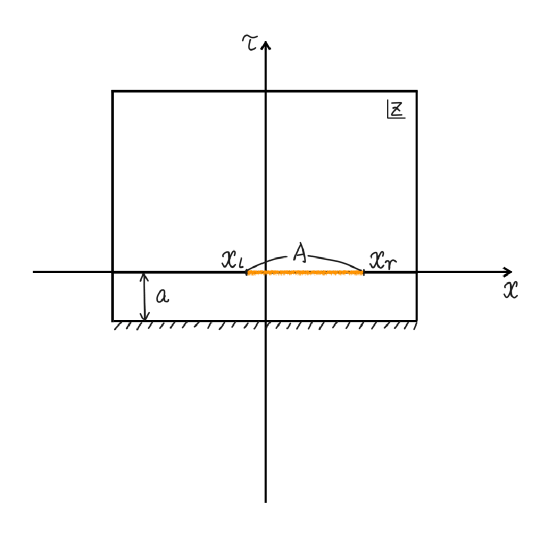
Refer to caption
Figure 20: The Euclidean path integral setup. The orange line shows the subsystem A𝐴A.

The minimal surface whose area computes holographic entanglement entropy can end on the end-of-the-world brane in AdS/BCFT [60]. Therefore, in the zero tension T=0𝑇0T=0 case, we have

SA=min{SAcon,SAdis}subscript𝑆𝐴superscriptsubscript𝑆𝐴𝑐𝑜𝑛superscriptsubscript𝑆𝐴𝑑𝑖𝑠\displaystyle S_{A}=\min\{S_{A}^{con},S_{A}^{dis}\} (5.33)
SAcon=c3loglϵsuperscriptsubscript𝑆𝐴𝑐𝑜𝑛𝑐3𝑙italic-ϵ\displaystyle S_{A}^{con}=\frac{c}{3}\log\frac{l}{\epsilon} (5.34)
SAdis=c3log2aϵsuperscriptsubscript𝑆𝐴𝑑𝑖𝑠𝑐32𝑎italic-ϵ\displaystyle S_{A}^{dis}=\frac{c}{3}\log\frac{2a}{\epsilon} (5.35)

where l𝑙l is the length of the subsystem A𝐴A and ϵitalic-ϵ\epsilon is the UV cutoff corresponding to the lattice distance. Figure 21 shows the ΔSAΔsubscript𝑆𝐴\Delta S_{A} for a subsystem A𝐴A with different length.

Refer to caption
Figure 21: ΔSAΔsubscript𝑆𝐴\Delta S_{A} for a subsystem A𝐴A with different length. Here, we set a=2𝑎2a=2.

Notice also in the limit a0𝑎0a\to 0, we obtain SAdissubscriptsuperscript𝑆𝑑𝑖𝑠𝐴S^{dis}_{A} by setting aϵsimilar-to𝑎italic-ϵa\sim\epsilon. This is consistent with (2.14) because the boundary state does not have any entanglement under a spacial decomposition [61].

5.6 Linearity of Holographic Pseudo Entropy

For CFT states dual to semiclassical geometries (holographic states), we expect the entanglement entropy can be approximated as an expectation value of the so-called area operator [29, 62, 63]. Let us consider the linear combination of holographic states,

|Ψi=k=1Mαik|ψik,ketsubscriptΨ𝑖subscriptsuperscript𝑀𝑘1subscript𝛼𝑖𝑘ketsubscript𝜓𝑖𝑘\ket{\Psi_{i}}=\sum^{M}_{k=1}\alpha_{ik}\ket{\psi_{ik}}, (5.36)

and its reduced density matrix ρAΨi=TrA¯|ΨiΨi|subscriptsuperscript𝜌subscriptΨ𝑖𝐴subscriptTr¯𝐴ketsubscriptΨ𝑖brasubscriptΨ𝑖\rho^{\Psi_{i}}_{A}=\mathrm{Tr}_{\bar{A}}\ket{\Psi_{i}}\bra{\Psi_{i}}. Then, the entanglement entropy gives

S(ρAΨi)Ψi|𝒜^4GN|ΨiΨi|Ψi=k=1M|αik|2A(ΓAψik)4GN,similar-to-or-equals𝑆subscriptsuperscript𝜌subscriptΨ𝑖𝐴brasubscriptΨ𝑖^𝒜4subscript𝐺𝑁ketsubscriptΨ𝑖inner-productsubscriptΨ𝑖subscriptΨ𝑖subscriptsuperscript𝑀𝑘1superscriptsubscript𝛼𝑖𝑘2AsubscriptsuperscriptΓsubscript𝜓𝑖𝑘𝐴4subscript𝐺𝑁S(\rho^{\Psi_{i}}_{A})\simeq\dfrac{\bra{\Psi_{i}}\frac{\hat{\mathcal{A}}}{4G_{N}}\ket{\Psi_{i}}}{\braket{\Psi_{i}}{\Psi_{i}}}=\sum^{M}_{k=1}|\alpha_{ik}|^{2}\dfrac{\mbox{A}(\Gamma^{\psi_{ik}}_{A})}{4G_{N}}, (5.37)

where A(ΓAψik)AsubscriptsuperscriptΓsubscript𝜓𝑖𝑘𝐴\mbox{A}(\Gamma^{\psi_{ik}}_{A}) corresponds to the area of the minimal surface (homologous to A𝐴A) in a geometry dual to a holographic state |ψikketsubscript𝜓𝑖𝑘\ket{\psi_{ik}}. Note that M𝑀M is supposed to be a small number compared with e𝒪(GN1)superscript𝑒𝒪superscriptsubscript𝐺𝑁1e^{\mathcal{O}{(G_{N}^{-1})}} [62]. We also assumed that ψik|ψi=δkinner-productsubscript𝜓𝑖𝑘subscript𝜓𝑖subscript𝛿𝑘\braket{\psi_{ik}}{\psi_{i\ell}}=\delta_{k\ell} and k|αik|2=1subscript𝑘superscriptsubscript𝛼𝑖𝑘21\sum_{k}|\alpha_{ik}|^{2}=1. We expect a version of the linearity of pseudo entropy for transition matrix 𝒯AΨi|Ψj=TrA¯|ΨiΨj|/Ψj|Ψisubscriptsuperscript𝒯conditionalsubscriptΨ𝑖subscriptΨ𝑗𝐴subscriptTr¯𝐴ketsubscriptΨ𝑖brasubscriptΨ𝑗inner-productsubscriptΨ𝑗subscriptΨ𝑖\mathcal{T}^{\Psi_{i}|\Psi_{j}}_{A}=\mathrm{Tr}_{\bar{A}}\ket{\Psi_{i}}\bra{\Psi_{j}}/\braket{\Psi_{j}}{\Psi_{i}},

S(𝒯AΨi|Ψj)Ψj|𝒜^4GN|ΨiΨj|Ψi=1kαjkαikkαjkαikA(ΓAψjk|ψik)4GN,similar-to-or-equals𝑆subscriptsuperscript𝒯conditionalsubscriptΨ𝑖subscriptΨ𝑗𝐴brasubscriptΨ𝑗^𝒜4subscript𝐺𝑁ketsubscriptΨ𝑖inner-productsubscriptΨ𝑗subscriptΨ𝑖1subscript𝑘subscriptsuperscript𝛼𝑗𝑘subscript𝛼𝑖𝑘subscript𝑘subscriptsuperscript𝛼𝑗𝑘subscript𝛼𝑖𝑘AsubscriptsuperscriptΓconditionalsubscript𝜓𝑗𝑘subscript𝜓𝑖𝑘𝐴4subscript𝐺𝑁S(\mathcal{T}^{\Psi_{i}|\Psi_{j}}_{A})\simeq\dfrac{\bra{\Psi_{j}}\frac{\hat{\mathcal{A}}}{4G_{N}}\ket{\Psi_{i}}}{\braket{\Psi_{j}}{\Psi_{i}}}=\frac{1}{\sum_{k}\alpha^{\ast}_{jk}\alpha_{ik}}\sum_{k}\alpha^{\ast}_{jk}\alpha_{ik}\dfrac{\mbox{A}(\Gamma^{{\psi_{jk}|\psi_{ik}}}_{A})}{4G_{N}}, (5.38)

where A(ΓAψjk|ψik)AsubscriptsuperscriptΓconditionalsubscript𝜓𝑗𝑘subscript𝜓𝑖𝑘𝐴\mbox{A}(\Gamma^{{\psi_{jk}|\psi_{ik}}}_{A}) corresponds to the minimal surface (homologous to A𝐴A) in a geometry dual to an inner product ψjk|ψikinner-productsubscript𝜓𝑗𝑘subscript𝜓𝑖𝑘\braket{\psi_{jk}}{\psi_{ik}}. It means that the holographic pseudo entropy computes a weak value of the area operator. Therefore, if one chooses coefficients ciksubscript𝑐𝑖𝑘c_{ik} and cjksubscript𝑐𝑗𝑘c_{jk} appropriately, like examples of qubit systems, one can easily obtain complex values even from holographic states. We leave a proof of (5.38) for linear combinations of so-called heavy states in appendix G.
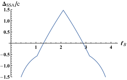
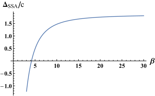
Refer to captionRefer to caption
Figure 22: Plots for ΔSSAsubscriptΔ𝑆𝑆𝐴\Delta_{SSA} (with the unit of the central charge c𝑐c) defined in (5.44). The regime ΔSSA>0subscriptΔ𝑆𝑆𝐴0\Delta_{SSA}>0 shows the breaking of strong subadditivity. For simplicity, we consider adjacent intervals: A=[0,π/3],B=[π/3,B],formulae-sequence𝐴0𝜋3𝐵𝜋3subscript𝐵A=[0,\pi/3],B=[\pi/3,\ell_{B}],and C=[B,B+π/3]𝐶subscript𝐵subscript𝐵𝜋3C=[\ell_{B},\ell_{B}+\pi/3]. Left panel: Bsubscript𝐵\ell_{B} dependence with βH1=1subscript𝛽subscript𝐻11\beta_{H_{1}}=1 and βH2=10subscript𝛽subscript𝐻210\beta_{H_{2}}=10. Note that this state satisfies both positivity and subadditivity of pseudo entropy. Right panel: βH2subscript𝛽subscript𝐻2\beta_{H_{2}} dependence with B=2π/3subscript𝐵2𝜋3\ell_{B}=2\pi/3 and βH1=1subscript𝛽subscript𝐻11\beta_{H_{1}}=1.

Here we just illustrate an example of the linear combination of holographic states which does break the strong subadditivity for pseudo entropy (5.6) even when we restrict to a canonical time slice for the definition of subsystems, while it holds the positivity. We focus on the two-dimensional holographic CFT on a cylinder with periodicity 2π2𝜋2\pi and take a given connected subsystem size as Asubscript𝐴\ell_{A}. Let us consider a superposition of two heavy states,

|Ψ±=15(|𝒪H1±2|𝒪H2),ketsubscriptΨplus-or-minus15plus-or-minusketsubscript𝒪subscript𝐻12ketsubscript𝒪subscript𝐻2\ket{\Psi_{\pm}}=\dfrac{1}{\sqrt{5}}(\ket{\mathcal{O}_{H_{1}}}\pm 2\ket{\mathcal{O}_{H_{2}}}), (5.39)

where each 𝒪Hisubscript𝒪subscript𝐻𝑖\mathcal{O}_{H_{i}} has the conformal dimension hHi=h¯Hi=𝒪(c)c24subscriptsubscript𝐻𝑖subscript¯subscript𝐻𝑖𝒪𝑐𝑐24h_{H_{i}}=\bar{h}_{H_{i}}=\mathcal{O}(c)\geq\frac{c}{24}.

The linearity relation (5.38) leads

S(𝒯AΨ+|Ψ)=53(A(ΓAH1)4GN+4A(ΓAH2)4GN),𝑆subscriptsuperscript𝒯conditionalsubscriptΨsubscriptΨ𝐴53AsubscriptsuperscriptΓsubscript𝐻1𝐴4subscript𝐺𝑁4AsubscriptsuperscriptΓsubscript𝐻2𝐴4subscript𝐺𝑁S(\mathcal{T}^{\Psi_{+}|\Psi_{-}}_{A})=\dfrac{5}{3}\left(-\dfrac{\mbox{A}(\Gamma^{H_{1}}_{A})}{4G_{N}}+4\dfrac{\mbox{A}(\Gamma^{H_{2}}_{A})}{4G_{N}}\right), (5.40)

where

𝒯AΨ+|Ψsubscriptsuperscript𝒯conditionalsubscriptΨsubscriptΨ𝐴\displaystyle\mathcal{T}^{\Psi_{+}|\Psi_{-}}_{A} =TrA¯|Ψ+Ψ|Ψ|Ψ+,absentsubscriptTr¯𝐴ketsubscriptΨbrasubscriptΨinner-productsubscriptΨsubscriptΨ\displaystyle=\mathrm{Tr}_{\bar{A}}\frac{\ket{\Psi_{+}}\bra{\Psi_{-}}}{\braket{\Psi_{-}}{\Psi_{+}}}, (5.41)
A(ΓAHi)4GNAsubscriptsuperscriptΓsubscript𝐻𝑖𝐴4subscript𝐺𝑁\displaystyle\dfrac{\mbox{A}(\Gamma^{H_{i}}_{A})}{4G_{N}} =c6log(βHiπϵsinh[πβHimin(A,2πA)]),absent𝑐6subscript𝛽subscript𝐻𝑖𝜋italic-ϵ𝜋subscript𝛽subscript𝐻𝑖minsubscript𝐴2𝜋subscript𝐴\displaystyle=\dfrac{c}{6}\log\left(\dfrac{\beta_{H_{i}}}{\pi\epsilon}\sinh\left[\dfrac{\pi}{\beta_{H_{i}}}\mathrm{min}(\ell_{A},2\pi-\ell_{A})\right]\right), (5.42)
βHisubscript𝛽subscript𝐻𝑖\displaystyle\beta_{H_{i}} =2π24hHic1.absent2𝜋24subscriptsubscript𝐻𝑖𝑐1\displaystyle=\dfrac{2\pi}{\sqrt{\frac{24h_{H_{i}}}{c}-1}}. (5.43)

Each area term describes the area of the minimal surfaces for (a micro state of) BTZ blackhole with the inverse temperature βHisubscript𝛽subscript𝐻𝑖\beta_{H_{i}}101010Strictly speaking, there is another phase for these pure states [64, 65]. In this paper, however, we neglect this phase just for simplicity.. Remarkably, this linear combination of holographic states leads the breaking of strong subadditivity for pseudo entropy, while we maintain the positivity S(𝒯AΨ+|Ψ)0𝑆subscriptsuperscript𝒯conditionalsubscriptΨsubscriptΨ𝐴0S(\mathcal{T}^{\Psi_{+}|\Psi_{-}}_{A})\geq 0, for example. To see this, let us define

ΔSSA=S(𝒯ABCΨi|Ψj)+S(𝒯BΨi|Ψj)S(𝒯ABΨi|Ψj)+S(𝒯BCΨi|Ψj).subscriptΔ𝑆𝑆𝐴𝑆subscriptsuperscript𝒯conditionalsubscriptΨ𝑖subscriptΨ𝑗𝐴𝐵𝐶𝑆subscriptsuperscript𝒯conditionalsubscriptΨ𝑖subscriptΨ𝑗𝐵𝑆subscriptsuperscript𝒯conditionalsubscriptΨ𝑖subscriptΨ𝑗𝐴𝐵𝑆subscriptsuperscript𝒯conditionalsubscriptΨ𝑖subscriptΨ𝑗𝐵𝐶\Delta_{SSA}=S(\mathcal{T}^{\Psi_{i}|\Psi_{j}}_{ABC})+S(\mathcal{T}^{\Psi_{i}|\Psi_{j}}_{B})-S(\mathcal{T}^{\Psi_{i}|\Psi_{j}}_{AB})+S(\mathcal{T}^{\Psi_{i}|\Psi_{j}}_{BC}). (5.44)

We plotted ΔSSAsubscriptΔ𝑆𝑆𝐴\Delta_{SSA} for our example in figure 22.

6 Generalizations for Operator and Mixed States

Finally, let us consider a possible generalization of the pseudo entropy for mixed states. So far, we have seen that the holographic pseudo entropy S(𝒯Aψ|φ)𝑆subscriptsuperscript𝒯conditional𝜓𝜑𝐴S(\mathcal{T}^{\psi|{\varphi}}_{A}) computes the minimal surfaces on the geometry associated with φ|ψinner-product𝜑𝜓\braket{{\varphi}}{\psi}. Based on this observation, it is natural to introduce some generalizations for mixed states which are holographically equivalent to entanglement wedge cross sections [66, 67] in the dual geometry. There are several proposals for mixed state measures dual to this cross-section [66, 67, 68, 69, 70, 71, 72], but here we define a generalization based on a canonical purification in [70].

6.1 Operator States for Transition Matrices

The entanglement entropy for a given purified density matrix can be regarded as a specific example of so-called operator entanglement entropy [73, 74] (see also [75, 76] for recent applications). Therefore, we first discuss its transition matrix and pseudo entropy counterpart. Let us start from an operator,

X=i,j[X]ij|iAjA|,𝑋subscript𝑖𝑗subscriptdelimited-[]𝑋𝑖𝑗ketsubscript𝑖𝐴brasubscript𝑗𝐴\displaystyle X=\sum_{i,j}[X]_{ij}\ket{i_{A}}\bra{j_{A}}, (6.1)

which is not necessarily to be Hermitian, XXsuperscript𝑋𝑋X^{\dagger}\neq X. We can define a corresponding operator state111111To avoid an unnecessarily ambiguity from unitary transformations, we further assume the above basis |iAketsubscript𝑖𝐴\ket{i_{A}} are product states. ,

|X=i,j[X]ij|iA|jA.ket𝑋subscript𝑖𝑗subscriptdelimited-[]𝑋𝑖𝑗ketsubscript𝑖𝐴ketsubscriptsuperscript𝑗superscript𝐴\displaystyle\ket{X}=\sum_{i,j}[X]_{ij}\ket{i_{A}}\ket{j^{\ast}_{A^{\ast}}}. (6.2)

where |jketsuperscript𝑗\ket{j^{\ast}} is a complex conjugate of |jket𝑗\ket{j}. Then, one can define any transition matrices for operator states and compute entanglement entropy for such transition matrices. From the next section, we are particularly interested in a specific case that our transition matrix121212In (6.3), we abused the notation of the transition matrix. In below, the operators assigned in the arguments of transition matrices will be assumed to be corresponding operator states. is given by

𝒯X|Xsuperscript𝒯conditional𝑋superscript𝑋\displaystyle\mathcal{T}^{X|X^{\dagger}} =|XX|X|X,absentket𝑋brasuperscript𝑋inner-productsuperscript𝑋𝑋\displaystyle=\dfrac{\ket{X}\bra{X^{\dagger}}}{\braket{X^{\dagger}}{X}}, (6.3)

where X𝑋X will be given by a transition matrix between two holographic states. Note that if we started from a Hermitian operator X𝑋X, this reduces to the usual operator entanglement for X𝑋X.

Before discussing the transition matrix as (6.3), it is rather natural to consider the ordinary operator entanglement for a single reduced transition matrix itself. In the rest part of this subsection, as a warmup exercise, we discuss entanglement entropy for a given operator state dual to a reduced transition matrix. The reader who is familiar with the reflected entropy may skip to the next subsection.

Starting from a given reduced transition matrix 𝒯Aψ|φsubscriptsuperscript𝒯conditional𝜓𝜑𝐴\mathcal{T}^{\psi|{\varphi}}_{A}, we can introduce a series of operator states,

|(𝒯Aψ|φ)m2=i,j[(𝒯Aψ|φ)m2]ij|iA|jA,ketsuperscriptsubscriptsuperscript𝒯conditional𝜓𝜑𝐴𝑚2subscript𝑖𝑗subscriptdelimited-[]superscriptsubscriptsuperscript𝒯conditional𝜓𝜑𝐴𝑚2𝑖𝑗ketsubscript𝑖𝐴ketsubscriptsuperscript𝑗superscript𝐴\ket{(\mathcal{T}^{\psi|{\varphi}}_{A})^{\frac{m}{2}}}=\sum_{i,j}[(\mathcal{T}^{\psi|{\varphi}}_{A})^{\frac{m}{2}}]_{ij}\ket{i_{A}}\ket{j^{\ast}_{A^{\ast}}}, (6.4)

where m𝑚m is assumed to be an even integer. We can then introduce reduced density matrices associated with these operator states,

ρA(m)=TrA|(𝒯Aψ|φ)m2(𝒯Aψ|φ)m2|.subscriptsuperscript𝜌𝑚𝐴subscriptTrsuperscript𝐴ketsuperscriptsubscriptsuperscript𝒯conditional𝜓𝜑𝐴𝑚2brasuperscriptsubscriptsuperscript𝒯conditional𝜓𝜑𝐴𝑚2\rho^{(m)}_{A}=\mathrm{Tr}_{A^{\ast}}\ket{(\mathcal{T}^{\psi|{\varphi}}_{A})^{\frac{m}{2}}}\bra{(\mathcal{T}^{\psi|{\varphi}}_{A})^{\frac{m}{2}}}. (6.5)

Note that we are loose about the normalization which will be taken into account later. In what follows, we focus on m1𝑚1m\rightarrow 1 limit where m𝑚m is an analytic continuation of an even integer.

If 𝒯Aψ|φsubscriptsuperscript𝒯conditional𝜓𝜑𝐴\mathcal{T}^{\psi|{\varphi}}_{A} is a physical state, nothing is what we did, just purifying and undoing a given state 𝒯Aψ|φsubscriptsuperscript𝒯conditional𝜓𝜑𝐴\mathcal{T}^{\psi|{\varphi}}_{A}. Therefore, in such cases, the pseudo entropy for 𝒯Aψ|φsubscriptsuperscript𝒯conditional𝜓𝜑𝐴\mathcal{T}^{\psi|{\varphi}}_{A} and the entanglement entropy for (6.5) (with m1𝑚1m\rightarrow 1) does match. A particularly interesting example is the class \mathscr{E} in two qubit systems (see around (3.49)) where we have a nice interpretation of the pseudo entropy as counting of Bell pairs. We stress that the transition matrices are not hermitian in general, hence the resulting physical state ρA(m)subscriptsuperscript𝜌𝑚𝐴\rho^{(m)}_{A} is not the original (𝒯Aψ|φ)msuperscriptsubscriptsuperscript𝒯conditional𝜓𝜑𝐴𝑚(\mathcal{T}^{\psi|{\varphi}}_{A})^{m} in general. We can easily confirm this discrepancy between ρA(m)subscriptsuperscript𝜌𝑚𝐴\rho^{(m)}_{A} and (𝒯Aψ|φ)msuperscriptsubscriptsuperscript𝒯conditional𝜓𝜑𝐴𝑚(\mathcal{T}^{\psi|{\varphi}}_{A})^{m} from the two qubit examples which are out of class 𝒟𝒟\mathscr{D}.

We can compute n𝑛n-th Rényi entropy for ρA(m)subscriptsuperscript𝜌𝑚𝐴\rho^{(m)}_{A} by using the standard replica trick. Figure 23 shows the replica manifold for [(𝒯Aψ|φ)m2]ij,[(𝒯Aψ|φ)m2]ij,subscriptdelimited-[]superscriptsubscriptsuperscript𝒯conditional𝜓𝜑𝐴𝑚2𝑖𝑗subscriptdelimited-[]superscriptsubscriptsuperscript𝒯conditional𝜓𝜑𝐴absent𝑚2𝑖𝑗[(\mathcal{T}^{\psi|{\varphi}}_{A})^{\frac{m}{2}}]_{ij},[(\mathcal{T}^{\psi|{\varphi}}_{A})^{\dagger\frac{m}{2}}]_{ij}, and [ρA(m)]ijsubscriptdelimited-[]subscriptsuperscript𝜌𝑚𝐴𝑖𝑗[\rho^{(m)}_{A}]_{ij}. In this case, the global structure of the replica manifold is the same as the ordinary n𝑛n-th Rényi entropy. Therefore, we can in principle reuse the replica trick calculations discussed in the previous sections. One main difference is that now we have two replica numbers m𝑚m and n𝑛n both of which will be taken to be one. From the next subsection, we move to the pseudo generalization of the reflected entropy, where we will use the similar replica trick described above with an extra complication due to topology of a replica manifold131313But with one simplification: since 𝒯Aψ|φsubscriptsuperscript𝒯conditional𝜓𝜑𝐴\mathcal{T}^{\psi|{\varphi}}_{A} is not Hermitian, there is no obvious 2subscript2\mathbb{Z}_{2} reflection symmetry in the n𝑛n-th Rényi entropy for ρA(m)subscriptsuperscript𝜌𝑚𝐴\rho^{(m)}_{A}. The lack of this symmetry causes difficulties to compute the replica partition function and to identify its bulk dual. We would like to come back this point in the future. In the next subsection, we construct a pseudo version of the reflected entropy such that we artificially hold this symmetry. It indeed makes our computation simpler. .
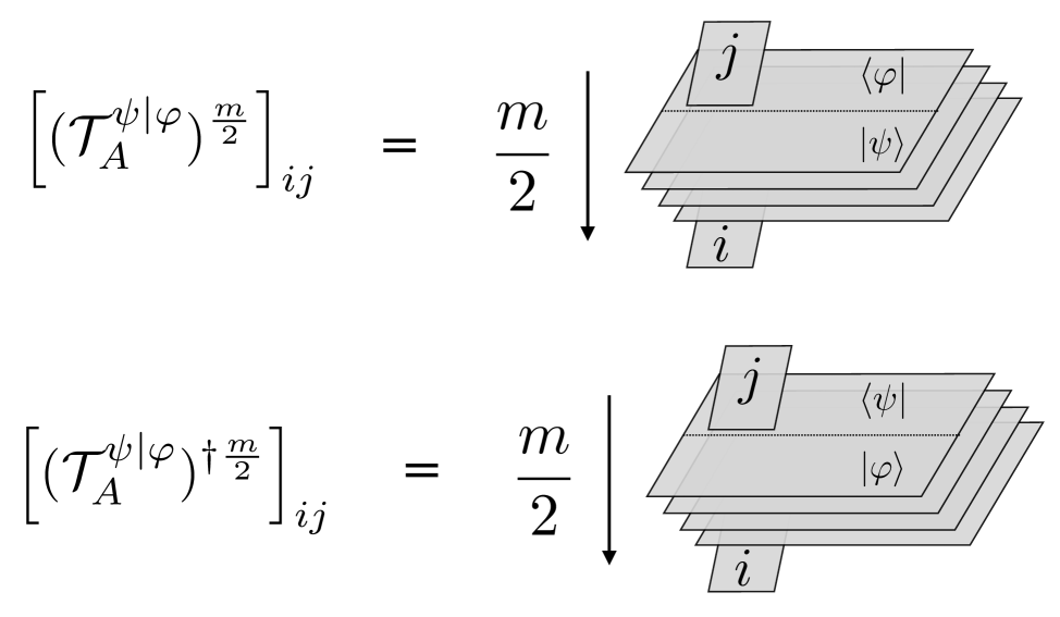
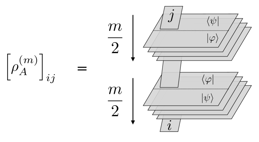
Refer to caption
Refer to caption
Figure 23: Left: replica manifolds for matrix elements of (𝒯Aψ|φ)m2superscriptsubscriptsuperscript𝒯conditional𝜓𝜑𝐴𝑚2(\mathcal{T}^{\psi|{\varphi}}_{A})^{\frac{m}{2}} and (𝒯Aψ|φ)m2superscriptsubscriptsuperscript𝒯conditional𝜓𝜑𝐴absent𝑚2(\mathcal{T}^{\psi|{\varphi}}_{A})^{\dagger\frac{m}{2}}. Right: One for ρA(m)subscriptsuperscript𝜌𝑚𝐴\rho^{(m)}_{A}. Here m𝑚m is assumed to be an even integer.

6.2 Pseudo Reflected Entropy

Based on the pseudo entropy for the operator states introduced in the previous subsection, let us define “pseudo reflected entropy” as

SR(𝒯ABψ|φ)=limm1limn1SR(n,m)(𝒯ABψ|φ),subscript𝑆𝑅subscriptsuperscript𝒯conditional𝜓𝜑𝐴𝐵subscript𝑚1subscript𝑛1subscriptsuperscript𝑆𝑛𝑚𝑅subscriptsuperscript𝒯conditional𝜓𝜑𝐴𝐵S_{R}(\mathcal{T}^{\psi|{\varphi}}_{AB})=\lim_{m\rightarrow 1}\lim_{n\rightarrow 1}S^{(n,m)}_{R}(\mathcal{T}^{\psi|{\varphi}}_{AB}), (6.6)

where

SR(n,m)(𝒯ABψ|φ)=S(n)(𝒯AA(𝒯ABψ|φ)m2|(𝒯ABψ|φ)m2).subscriptsuperscript𝑆𝑛𝑚𝑅subscriptsuperscript𝒯conditional𝜓𝜑𝐴𝐵superscript𝑆𝑛subscriptsuperscript𝒯conditionalsuperscriptsubscriptsuperscript𝒯conditional𝜓𝜑𝐴𝐵𝑚2superscriptsubscriptsuperscript𝒯conditional𝜓𝜑𝐴𝐵𝑚2𝐴superscript𝐴S^{(n,m)}_{R}(\mathcal{T}^{\psi|{\varphi}}_{AB})=S^{(n)}(\mathcal{T}^{(\mathcal{T}^{\psi|{\varphi}}_{AB})^{\frac{m}{2}}|(\mathcal{T}^{\psi|{\varphi}\,\dagger}_{AB})^{\frac{m}{2}}}_{AA^{\ast}}). (6.7)

As like the original reflected entropy, we assumed that m𝑚m is an analytic continuation of an even integer.

In particular, if B=A¯𝐵¯𝐴B=\bar{A},

𝒯AA¯ψ|φ𝒯ψ|φ=|ψφ|φ|ψ,subscriptsuperscript𝒯conditional𝜓𝜑𝐴¯𝐴superscript𝒯conditional𝜓𝜑ket𝜓bra𝜑inner-product𝜑𝜓\mathcal{T}^{\psi|{\varphi}}_{A\bar{A}}\equiv\mathcal{T}^{\psi|{\varphi}}=\dfrac{\ket{\psi}\bra{{\varphi}}}{\braket{{\varphi}}{\psi}}, (6.8)

the pseudo reflected entropy SR(𝒯AA¯ψ|φ)subscript𝑆𝑅subscriptsuperscript𝒯conditional𝜓𝜑𝐴¯𝐴S_{R}(\mathcal{T}^{\psi|{\varphi}}_{A\bar{A}}) reduces to the double of pseudo entropy,

SR(𝒯AA¯ψ|φ)=S(𝒯Aψ|φ)+S((𝒯Aψ|φ)T)=2S(𝒯Aψ|φ).subscript𝑆𝑅subscriptsuperscript𝒯conditional𝜓𝜑𝐴¯𝐴𝑆subscriptsuperscript𝒯conditional𝜓𝜑𝐴𝑆superscriptsubscriptsuperscript𝒯conditional𝜓𝜑𝐴𝑇2𝑆subscriptsuperscript𝒯conditional𝜓𝜑𝐴S_{R}(\mathcal{T}^{\psi|{\varphi}}_{A\bar{A}})=S(\mathcal{T}^{\psi|{\varphi}}_{A})+S((\mathcal{T}^{\psi|{\varphi}}_{A})^{T})=2S(\mathcal{T}^{\psi|{\varphi}}_{A}). (6.9)

In this sense, the pseudo reflected entropy gives a generalization of the pseudo entropy for mixed states. We will argue that holographic pseudo reflected entropy gives (double of) the entanglement wedge cross section on the geometry dual to φ|ψinner-product𝜑𝜓\braket{{\varphi}}{\psi},

SR(𝒯ABψ|φ)=2EW(𝒯ABψ|φ).subscript𝑆𝑅subscriptsuperscript𝒯conditional𝜓𝜑𝐴𝐵2subscript𝐸𝑊subscriptsuperscript𝒯conditional𝜓𝜑𝐴𝐵S_{R}(\mathcal{T}^{\psi|{\varphi}}_{AB})=2E_{W}(\mathcal{T}^{\psi|{\varphi}}_{AB}). (6.10)

We again stress that this definition is different from the usual operator entanglement for the transition matrix (𝒯ψ|φ)12superscriptsuperscript𝒯conditional𝜓𝜑12(\mathcal{T}^{\psi|{\varphi}})^{\frac{1}{2}}. For example, taking Hermitian conjugate for one of two X𝑋X in (6.2) is crucial to obtain the desired pure state limit in (6.9).

6.3 Replica Trick
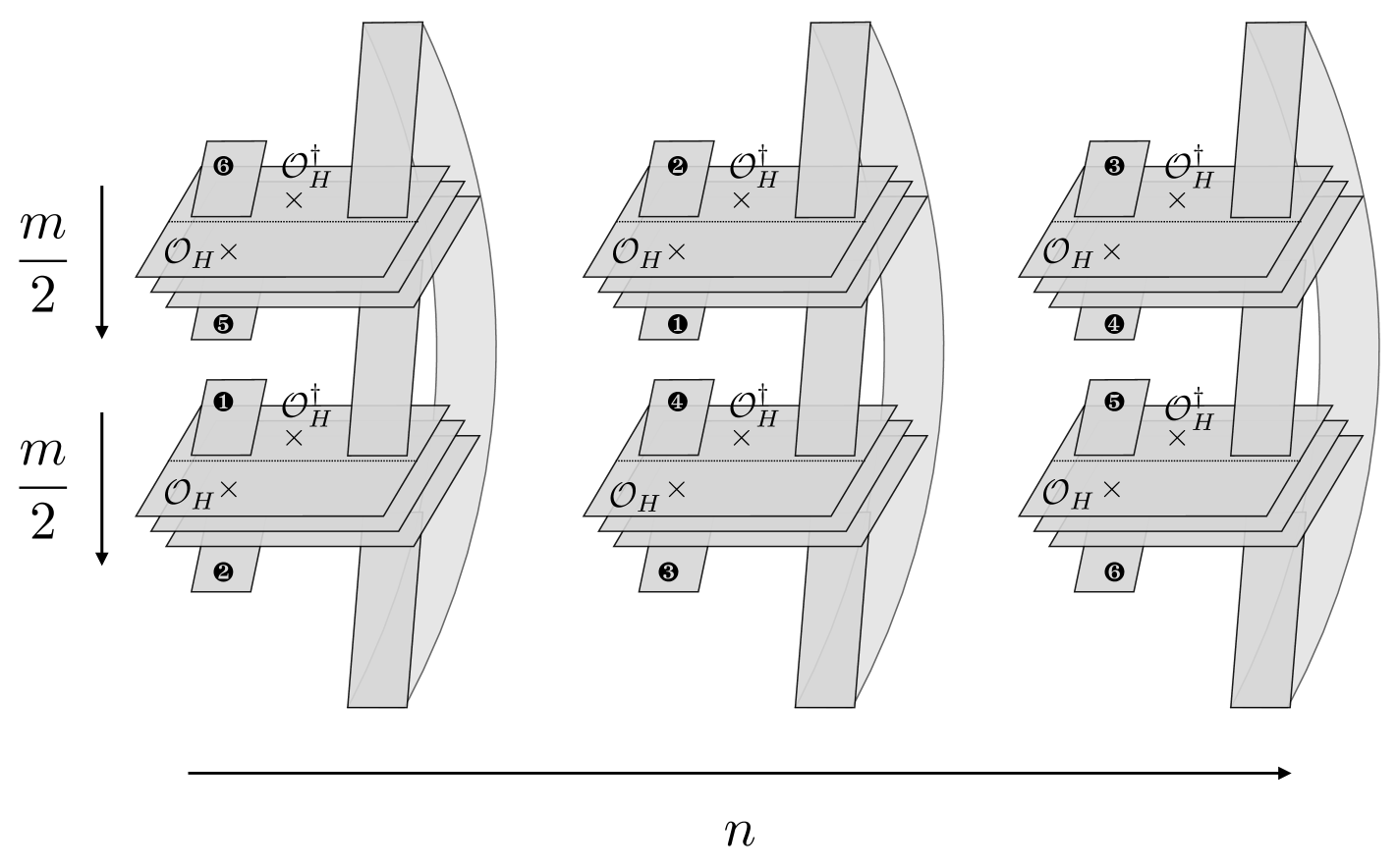
Refer to caption
Figure 24: Replica manifold for computing Zm,nsubscript𝑍𝑚𝑛Z_{m,n}. (The figure shows the n=3𝑛3n=3 case.) Each fixed n𝑛n corresponds to 𝒯AA(m)TrBB𝒯X|Xsubscriptsuperscript𝒯𝑚𝐴superscript𝐴subscriptTr𝐵superscript𝐵superscript𝒯conditional𝑋superscript𝑋\mathcal{T}^{(m)}_{AA^{\ast}}\equiv\mathrm{Tr}_{BB^{\ast}}\mathcal{T}^{X|X^{\dagger}} with X=(𝒯ABψ|φ)m2𝑋superscriptsubscriptsuperscript𝒯conditional𝜓𝜑𝐴𝐵𝑚2X=(\mathcal{T}^{\psi|{\varphi}}_{AB})^{\frac{m}{2}},  (|XAABB=|(𝒯ABψ|φ)m2ketsubscript𝑋𝐴superscript𝐴𝐵superscript𝐵ketsuperscriptsubscriptsuperscript𝒯conditional𝜓𝜑𝐴𝐵𝑚2\ket{X_{AA^{\ast}BB^{\ast}}}=\ket{(\mathcal{T}^{\psi|{\varphi}}_{AB})^{\frac{m}{2}}}). We glue each label in the figure (each circled number with black background) such that we obtain Tr(𝒯AA(m))nTrsuperscriptsubscriptsuperscript𝒯𝑚𝐴superscript𝐴𝑛\mathrm{Tr}(\mathcal{T}^{(m)}_{AA^{\ast}})^{n}. It can be rewritten as the correlator of twist operators as (6.19).

One of the main advantage of reflected entropy is that it can be computed using the correlation function of certain twist operators via the replica trick [70, 64, 65]. This is also the case for the pseudo reflected entropy. For concreteness, let us consider a reduced transition matrix obtained from two excited states,

𝒯ABψ|φ=TrAB¯(|ψφ|φ|ψ),subscriptsuperscript𝒯conditional𝜓𝜑𝐴𝐵subscriptTr¯𝐴𝐵ket𝜓bra𝜑inner-product𝜑𝜓\mathcal{T}^{\psi|{\varphi}}_{AB}=\mathrm{Tr}_{\overline{AB}}\left(\frac{\ket{\psi}\bra{{\varphi}}}{\braket{{\varphi}}{\psi}}\right), (6.11)

where

|ψ=𝒪H(w5,w¯5)|0,|φ=𝒪H(w0,w¯0)|0.formulae-sequenceket𝜓subscript𝒪𝐻subscript𝑤5subscript¯𝑤5ket0ket𝜑subscript𝒪𝐻subscript𝑤0subscript¯𝑤0ket0\ket{\psi}=\mathcal{O}_{H}(w_{5},\bar{w}_{5})\ket{0},\;\ket{{\varphi}}=\mathcal{O}_{H}(w_{0},\bar{w}_{0})\ket{0}. (6.12)

We will specify the conformal dimension later. Here we took subregions as A=[w1,w2]𝐴subscript𝑤1subscript𝑤2A=[w_{1},w_{2}], B=[w3,w4]𝐵subscript𝑤3subscript𝑤4B=[w_{3},w_{4}] and set

w1subscript𝑤1\displaystyle w_{1} =w¯1=u1,w2=w¯2=v1,w3=w¯3=u2,w4=w¯4=v2,formulae-sequenceabsentsubscript¯𝑤1subscript𝑢1subscript𝑤2subscript¯𝑤2subscript𝑣1subscript𝑤3subscript¯𝑤3subscript𝑢2subscript𝑤4subscript¯𝑤4subscript𝑣2\displaystyle=\bar{w}_{1}=u_{1},\,w_{2}=\bar{w}_{2}=v_{1},\,w_{3}=\bar{w}_{3}=u_{2},\,w_{4}=\bar{w}_{4}=v_{2}, (6.13)
w0subscript𝑤0\displaystyle w_{0} =a2+ib2,w¯0=a2ib2,w5=a1ib1,w¯5=a1+ib1,formulae-sequenceabsentsubscript𝑎2𝑖subscript𝑏2formulae-sequencesubscript¯𝑤0subscript𝑎2𝑖subscript𝑏2formulae-sequencesubscript𝑤5subscript𝑎1𝑖subscript𝑏1subscript¯𝑤5subscript𝑎1𝑖subscript𝑏1\displaystyle=a_{2}+ib_{2},\bar{w}_{0}=a_{2}-ib_{2},w_{5}=a_{1}-ib_{1},\bar{w}_{5}=a_{1}+ib_{1}, (6.14)

Based on [70], it is straightforward to construct the replica partition function for a series of canonically purified states. One can define the Rényi version of the reflected entropy as,

SR(n,m)subscriptsuperscript𝑆𝑛𝑚𝑅\displaystyle S^{(n,m)}_{R} =11nlogZm,n(Zm,1)n,absent11𝑛subscript𝑍𝑚𝑛superscriptsubscript𝑍𝑚1𝑛\displaystyle=\dfrac{1}{1-n}\log\dfrac{Z_{m,n}}{(Z_{m,1})^{n}}, (6.15)

where

Zm,nsubscript𝑍𝑚𝑛\displaystyle Z_{m,n} =Tr(𝒯AA(m))n,absentTrsuperscriptsubscriptsuperscript𝒯𝑚𝐴superscript𝐴𝑛\displaystyle=\mathrm{Tr}(\mathcal{T}^{(m)}_{AA^{\ast}})^{n}, (6.16)
𝒯AA(m)subscriptsuperscript𝒯𝑚𝐴superscript𝐴\displaystyle\mathcal{T}^{(m)}_{AA^{\ast}} =TrBB[|(𝒯ABψ|φ)m2(𝒯ABψ|φ)m2|(𝒯ψφAB)m2|(𝒯ABψ|φ)m2|missing].\displaystyle=\mathrm{Tr}_{BB^{\ast}}\left[\frac{\ket{(\mathcal{T}^{\psi|{\varphi}}_{AB})^{\frac{m}{2}}}\bra{(\mathcal{T}^{\psi|{\varphi}\,\dagger}_{AB})^{\frac{m}{2}}}}{\braket{(\mathcal{T}^{\psi}{{\varphi}\,\dagger}_{AB})^{\frac{m}{2}}}{(\mathcal{T}^{\psi|{\varphi}}_{AB})^{\frac{m}{2}}}{missing}}\right]. (6.17)

The Zm,nsubscript𝑍𝑚𝑛Z_{m,n} corresponds to a partition function on the manifold described in figure 24. Notice that each replica sheet represents the same one thanks to the Hermitian conjugate in (6.17). From (6.15), one can obtain

SR(𝒯ABψ|φ)=limm1limn111nlogZm,n(Zm,1)n,subscript𝑆𝑅subscriptsuperscript𝒯conditional𝜓𝜑𝐴𝐵subscript𝑚1subscript𝑛111𝑛subscript𝑍𝑚𝑛superscriptsubscript𝑍𝑚1𝑛S_{R}(\mathcal{T}^{\psi|{\varphi}}_{AB})=\lim_{m\rightarrow 1}\lim_{n\rightarrow 1}\dfrac{1}{1-n}\log\dfrac{Z_{m,n}}{(Z_{m,1})^{n}}, (6.18)

In particular, here we took an analytic continuation of an even integer m𝑚m. We can rewrite the Zm,nsubscript𝑍𝑚𝑛Z_{m,n} in terms of the correlation function of twist operators,

Zm,nsubscript𝑍𝑚𝑛\displaystyle Z_{m,n} =0|𝒪Hmn(w0,w¯0)σgA(u1)σgA1(v1)σgB(u2)σgB1(v2)𝒪Hmn(w5,w¯5)|0,absentquantum-operator-product0subscriptsuperscript𝒪tensor-productabsent𝑚𝑛𝐻subscript𝑤0subscript¯𝑤0subscript𝜎subscript𝑔𝐴subscript𝑢1subscript𝜎superscriptsubscript𝑔𝐴1subscript𝑣1subscript𝜎subscript𝑔𝐵subscript𝑢2subscript𝜎superscriptsubscript𝑔𝐵1subscript𝑣2subscriptsuperscript𝒪tensor-productabsent𝑚𝑛𝐻subscript𝑤5subscript¯𝑤50\displaystyle=\braket{0}{\mathcal{O}^{\otimes mn\dagger}_{H}(w_{0},\bar{w}_{0})\sigma_{g_{A}}(u_{1})\sigma_{g_{A}^{-1}}(v_{1})\sigma_{g_{B}}(u_{2})\sigma_{g_{B}^{-1}}(v_{2})\mathcal{O}^{\otimes mn}_{H}(w_{5},\bar{w}_{5})}{0}, (6.19)

where we have twist operators whose chiral conformal dimensions are given by hσgA=hσgA1=hσgB=hσgB1=nc24(m1m)nhmsubscriptsubscript𝜎subscript𝑔𝐴subscriptsubscript𝜎superscriptsubscript𝑔𝐴1subscriptsubscript𝜎subscript𝑔𝐵subscriptsubscript𝜎superscriptsubscript𝑔𝐵1𝑛𝑐24𝑚1𝑚𝑛subscript𝑚h_{\sigma_{g_{A}}}=h_{\sigma_{g_{A}^{-1}}}=h_{\sigma_{g_{B}}}=h_{\sigma_{g_{B}^{-1}}}=\frac{nc}{24}\left(m-\frac{1}{m}\right)\equiv nh_{m}, so as anti-chiral ones. These twist operators are essentially different from the ones appeared in the entanglement entropy because the global structure of the replica manifold is totally different. As a consequences of this difference, we have a particularly important OPE channel,

σgA1σgBσgBgA1+,similar-tosubscript𝜎superscriptsubscript𝑔𝐴1subscript𝜎subscript𝑔𝐵subscript𝜎subscript𝑔𝐵superscriptsubscript𝑔𝐴1\sigma_{g_{A}^{-1}}\sigma_{g_{B}}\sim\sigma_{g_{B}g_{A}^{-1}}+\cdots, (6.20)

where σgBgA1subscript𝜎subscript𝑔𝐵superscriptsubscript𝑔𝐴1\sigma_{g_{B}g_{A}^{-1}} has the conformal dimension hσgBgA1=h¯σgBgA1=2c24(n1n)2hnsubscriptsubscript𝜎subscript𝑔𝐵superscriptsubscript𝑔𝐴1subscript¯subscript𝜎subscript𝑔𝐵superscriptsubscript𝑔𝐴12𝑐24𝑛1𝑛2subscript𝑛h_{\sigma_{g_{B}g_{A}^{-1}}}=\bar{h}_{\sigma_{g_{B}g_{A}^{-1}}}=\frac{2c}{24}\left(n-\frac{1}{n}\right)\equiv 2h_{n}. Notice that this is the same correlation function as one for the reflected entropy [64, 65] except for the position of two operators 𝒪Hsubscript𝒪𝐻\mathcal{O}_{H} and 𝒪Hsubscriptsuperscript𝒪𝐻\mathcal{O}^{\dagger}_{H}.

6.4 Pseudo Reflected Entropy in Holographic CFT

Let us focus our analysis on the holographic CFT2. We specify two excited states in transition matrix with heavy states whose conformal dimensions are given by hH=h¯H=𝒪(c)c24subscript𝐻subscript¯𝐻𝒪𝑐𝑐24h_{H}=\bar{h}_{H}=\mathcal{O}(c)\geq\frac{c}{24}. In holographic CFT2, the correlation functions are well-approximated by the single conformal block. The 666-point correlation functions of our interest are often referred as heavy-heavy-light-light-light-light (HHLLLL) correlation functions, whose conformal blocks under the large c𝑐c limit are studied in literature. We apply a conformal map from cylinder to plane,

z=eiw~,w~=ww5ww0,formulae-sequence𝑧superscript𝑒𝑖~𝑤~𝑤𝑤subscript𝑤5𝑤subscript𝑤0z=e^{-i\tilde{w}},\;\tilde{w}=\dfrac{w-w_{5}}{w-w_{0}}, (6.21)

so that we get familiar forms of HHLLLL blocks in literature (refer to [77, 78] where the related conformal blocks are presented explicitly).
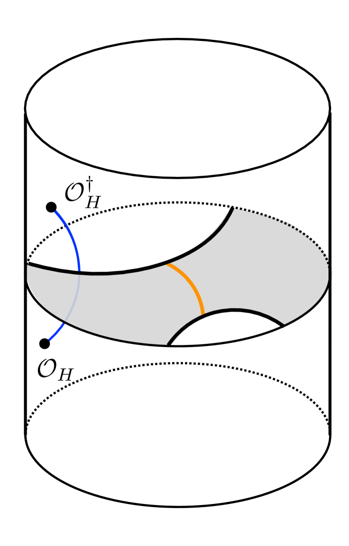
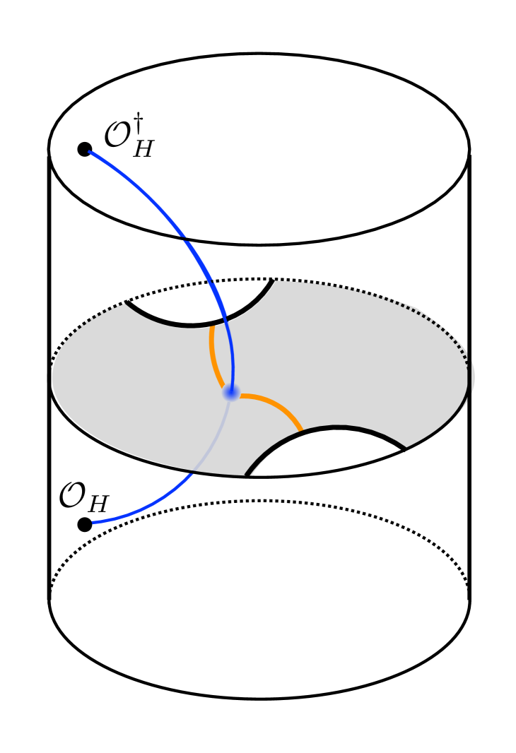
Refer to captionRefer to caption
Figure 25: Two typical phases for the entanglement wedge cross section in the geometry dual to φ|ψinner-product𝜑𝜓\braket{{\varphi}}{\psi}. Left: a connected cross section. Right: a disconnected cross section. Here we skip intermediate phases between left and right panels where we have transition of the entanglement wedge itself.

We have essentially two classes of non-zero entanglement wedge cross section. We can classify them with respect to whether the resulting cross sections have disconnected pieces or not. We will call these classes as disconnected or connected phases. The simplest cross section in the connected phase accords with one in the BTZ blackhole (see left panel of figure 25),

SR(𝒯ABψ|φ)=c6logcoth(αx4)+(anti-holomorphic),subscript𝑆𝑅subscriptsuperscript𝒯conditional𝜓𝜑𝐴𝐵𝑐6hyperbolic-cotangent𝛼𝑥4anti-holomorphicS_{R}(\mathcal{T}^{\psi|{\varphi}}_{AB})=\dfrac{c}{6}\log\coth\left(\dfrac{\alpha x}{4}\right)+(\textrm{anti-holomorphic}), (6.22)

where the cross ratios x,x¯𝑥¯𝑥x,\bar{x} are given by

x=(w~1w~2)(w~3w~4)(w~1w~3)(w~2w~4)=(u1v1)(u2v2)(u1u2)(v1v2)=x¯,𝑥subscript~𝑤1subscript~𝑤2subscript~𝑤3subscript~𝑤4subscript~𝑤1subscript~𝑤3subscript~𝑤2subscript~𝑤4subscript𝑢1subscript𝑣1subscript𝑢2subscript𝑣2subscript𝑢1subscript𝑢2subscript𝑣1subscript𝑣2¯𝑥x=\frac{(\tilde{w}_{1}-\tilde{w}_{2})(\tilde{w}_{3}-\tilde{w}_{4})}{(\tilde{w}_{1}-\tilde{w}_{3})(\tilde{w}_{2}-\tilde{w}_{4})}=\frac{(u_{1}-v_{1})(u_{2}-v_{2})}{(u_{1}-u_{2})(v_{1}-v_{2})}=\bar{x}, (6.23)

and

α=2π24hHc1.𝛼2𝜋24subscript𝐻𝑐1\alpha=\frac{2\pi}{\sqrt{\frac{24h_{H}}{c}-1}}. (6.24)

Therefore, this cross section does not depend on the location of heavy states in the Euclidian manifold. It is rather natural—because except for back reaction of the geometry, the cross section has no direct connection with the geodesics created by the heavy operators.

For sufficiently large subsystems, we reach the disconnected phase, where the cross section consists of two disconnected contributions both of which end at the horizon of blackhole (see right panel of figure 25),

SR(𝒯ABψ|φ)=c6logcoth(αx144)+c6logcoth(αx234)+(anti-holomorphic).subscript𝑆𝑅subscriptsuperscript𝒯conditional𝜓𝜑𝐴𝐵𝑐6hyperbolic-cotangent𝛼subscript𝑥144𝑐6hyperbolic-cotangent𝛼subscript𝑥234anti-holomorphicS_{R}(\mathcal{T}^{\psi|{\varphi}}_{AB})=\dfrac{c}{6}\log\coth\left(\dfrac{\alpha x_{14}}{4}\right)+\dfrac{c}{6}\log\coth\left(\dfrac{\alpha x_{23}}{4}\right)+(\textrm{anti-holomorphic}). (6.25)

where

x14=(w1w4)(w0w5)(w1w0)(w2w0),x23=(w2w3)(w0w5)(w2w0)(w3w0),formulae-sequencesubscript𝑥14subscript𝑤1subscript𝑤4subscript𝑤0subscript𝑤5subscript𝑤1subscript𝑤0subscript𝑤2subscript𝑤0subscript𝑥23subscript𝑤2subscript𝑤3subscript𝑤0subscript𝑤5subscript𝑤2subscript𝑤0subscript𝑤3subscript𝑤0x_{14}=\dfrac{(w_{1}-w_{4})(w_{0}-w_{5})}{(w_{1}-w_{0})(w_{2}-w_{0})},\;x_{23}=\dfrac{(w_{2}-w_{3})(w_{0}-w_{5})}{(w_{2}-w_{0})(w_{3}-w_{0})}, (6.26)

so as anti-holomorphic ones, x¯14subscript¯𝑥14\bar{x}_{14} and x¯23subscript¯𝑥23\bar{x}_{23}. These results are consistent with the entanglement wedge cross section as is obvious from the related conformal blocks.

7 Conclusions and Discussions

In this paper, we introduced a novel quantity called pseudo entropy motivated by a natural question in AdS/CFT: what is the CFT quantity dual to the minimal codimension-2 surface in the bulk AdS which ends on the boundary when there is no time reversal symmetry. A Euclidean path integral with time reversal symmetry in CFT gives a density matrix, while that without time reversal symmetry can be regarded as a transition matrix. A minimal codimension-2 surface anchored on a time reversal symmetric time slice gives the entanglement entropy of a reduced density matrix while that does not lie on such a time slice gives the pseudo entropy of a reduced transition matrix. In this sense, pseudo entropy is a straightforward generalization of entanglement entropy.

We studied general properties of pseudo entropy in section 2 and then focused on plenty of explicit examples in qubit systems, free CFT, and holographic setups in section 3, 4, 5. In section 6, we introduced the pseudo reflected entropy based on the pseudo entropy for the operator state. In particular, we argued it is equivalent to double of the entanglement wedge cross section in the dual geometry.

Pseudo entropy, introduced in the present paper with the above motivation and calculations, is a new fundamental quantity defined for any quantum systems. Therefore we expect this to open new directions to study quantum information theory, condensed matter physics and high energy theory. Below we summarize our conclusions on these analysis in more details as well as future problems from a comprehensive point of view.

Pseudo Entropy in Qubit Systems and Operational Meaning

We classified the structure of two qubit transition matrices with the relation to pseudo entropy in figure 3. In general, the transition matrices 𝒯Aψ|φsubscriptsuperscript𝒯conditional𝜓𝜑𝐴{\mathcal{T}}^{\psi|{\varphi}}_{A} are not Hermitian and are not regular quantum states, which lead to complex values of pseudo entropy in general. Nevertheless, this quantity shares several properties common also to entanglement entropy. We also uncovered several useful behaviors of pseudo entropy in qubit systems. In two qubit systems, we find that the pseudo entropy always gets increased under local unitary transformations. However, this is only a special property of two qubit systems, and we find the pseudo entropy in general gets reduced under local unitary transformations in larger systems especially when the entanglement swapping occurs. We observed this kind of reductions of pseudo entropy in a number of our examples in CFTs.

We then focus on the class \mathscr{B}, i.e. the case where the pseudo (Rényi) entropies are all real and non-negative. Our CFT examples in this paper fit into this class. In particular, when the reduced transition matrices 𝒯Aψ|φsubscriptsuperscript𝒯conditional𝜓𝜑𝐴{\mathcal{T}}^{\psi|{\varphi}}_{A} and 𝒯Bψ|φsubscriptsuperscript𝒯conditional𝜓𝜑𝐵{\mathcal{T}}^{\psi|{\varphi}}_{B} are Hermitian and positive semi-definite (i.e. the class \mathscr{E}), we showed that the pseudo entropy can be interpreted as the averaged number of Bell pairs included in intermediate states between the initial state and final state. This allows us to quantitatively investigate the amount of virtual entanglement involved in the post-selection process. It will be of interest to consider what physical phenomena follow from the virtual entanglement behind a given process. It is also important to know how to measure pseudo entropy in real experiments, and to provide a similar interpretation of pseudo entropy for general transition matrices.

We have also investigated the pseudo entropy when both |ψket𝜓\ket{\psi} and |φket𝜑\ket{{\varphi}} are chosen uniformly at random from the whole Hilbert space. It was observed that the pseudo entropy seems to weakly concentrate around a moderately small real value. This may indicate that, despite the facts that pseudo entropy is in general complex-valued and that its absolute value can be arbitrarily large, it is atypical for states to take such abnormal values of pseudo entropy, especially in the large dimension limit.

Holographic Pseudo Entropy

Our main motivation of considering pseudo entropy is the holographic duality. For a generic transition matrix and a generic factorization of the Hilbert space, pseudo entropy takes complex values. However, as we have seen in section 5.1, holographic pseudo n𝑛n-th Rényi entropy is nonnegative for any n>0𝑛0n>0, assuming a single classical gravity background with a real valued bulk metric. This gives rather strong restrictions since this implies that, no matter what spatial factorization we take for the whole Hilbert space, the reduced transition matrix should belong to class \mathscr{B}.

Moreover, one may also go further to expect that the reduced transition matrices in holographic setups have only real and nonnegative eigenvalues, i.e. they belong to class 𝒞𝒞\mathscr{C}. One way to check this expectation would be to evaluate weak values of observables other than the area operator. This is also left as a future problem.

Nevertheless, holographic transition matrix generically do not give Hermitian reduced transition matrices and hence do not belong to 𝒟𝒟\mathscr{D}. Indeed, it is straightforward to explicitly check Tr[(𝒯Aψ|φ)2]Tr[𝒯Aψ|φ(𝒯Aψ|φ)]Trdelimited-[]superscriptsubscriptsuperscript𝒯conditional𝜓𝜑𝐴2Trdelimited-[]subscriptsuperscript𝒯conditional𝜓𝜑𝐴superscriptsubscriptsuperscript𝒯conditional𝜓𝜑𝐴\mathrm{Tr}\left[\left({\mathcal{T}}^{\psi|{\varphi}}_{A}\right)^{2}\right]\neq\mathrm{Tr}\left[{\mathcal{T}}^{\psi|{\varphi}}_{A}\left({\mathcal{T}}^{\psi|{\varphi}}_{A}\right)^{\dagger}\right] and hence 𝒯Aψ|φ(𝒯Aψ|φ)subscriptsuperscript𝒯conditional𝜓𝜑𝐴superscriptsubscriptsuperscript𝒯conditional𝜓𝜑𝐴{\mathcal{T}}^{\psi|{\varphi}}_{A}\neq\left({\mathcal{T}}^{\psi|{\varphi}}_{A}\right)^{\dagger}.

As one of the simplest examples,we compute the holographic pseudo entropy explicitly for the Janus solution in AdS/3{}_{3}/CFT2, which is dual to two quantum states given by two different exactly marginal deformations. We showed that the coefficient of the logarithmic divergence of the pseudo entropy is decreased by the Janus perturbation and that the perturbative analysis in the dual field theory correctly reproduces this behavior.

Also, we found that transition matrices between two linear combinations of holographic states are even out of class 𝒜𝒜\mathscr{A} in general as we have seen in section 5.6. In the AdS/CFT, this is dual to a quantum mechanical superposition of two different classical gravity duals. We showed that in this general case, the holographic pseudo entropy is equal to the weak value of the area operator and this possesses the linearity property.

Since holographic pseudo entropy is a codimension-2 surface in the bulk, we also expect that it is possible to account for the holographic pseudo entropy as Hayward term or gravity edge modes [79, 80] if we focus on the fixed-area contribution and whether the basis for fixed area-states is universal or not.

Comparisons of Pseudo Entropy in Free and Holographic CFTs

We found the class \mathscr{B} property (i.e. all pseudo Rényi entropies take non-negative real values) arises naturally in general field theories when we prepare the two states |ψket𝜓|\psi\rangle and |φket𝜑|{\varphi}\rangle by Euclidean path-integrals. It is obvious that the transition matrices constructed by Euclidean path-integrals with real valued action and external sources at least belong to the class 𝒜𝒜\mathscr{A} because the transition matrices themselves are also real valued. In addition, Tr(𝒯Aψ|φ)n>0Trsuperscriptsubscriptsuperscript𝒯conditional𝜓𝜑𝐴𝑛0{\mathrm{Tr}\left({\mathcal{T}}^{\psi|{\varphi}}_{A}\right)^{n}}>0 for any n>0𝑛0n>0 in this special case. This means that the pseudo Rényi entropies are real valued. Moreover, we found in our explicit examples that the resulting pseudo entropy is non-negative. Indeed, the pseudo entropy typically follows the area law as in the standard entanglement entropy in field theories [6, 7]. In the two dimensional massless free scalar CFT, we calculated pseudo Rényi entropies when |ψket𝜓|\psi\rangle and |φket𝜑|{\varphi}\rangle are (different) locally excited states and found real valued pseudo entropy. In this free theory example, we always find that the pseudo entropy gets smaller than that for the ground state. In particular, the pseudo entropy is reduced sharply when the positions of the local operator excitations get closer to the boundaries of the subsystem A𝐴A. We interpret this behavior as the reduction of pseudo entropy in the presence of the entanglement swapping.

We studied the pseudo entropy for similar locally excited states in holographic CFTs. We again found the reduction of pseudo entropy when the positions of the local operators are close to the boundaries of the subsystem. Moreover, as opposed to the results in free CFTs, we observed that the holographic pseudo entropy can also increase when the local excitation is close to the center of the subsystem. This positive contribution seems to be a special feature of holographic CFTs, which is missing in free CFTs. It is a long-standing question what kinds of quantum states admit classical geometry duals and there are many known restrictions characterizing these states such as the monogamy of mutual information [81], holographic entropy cone [82] and holographic entropy arrangement [83]. For the behaviors of entanglement entropy under local excitations, it is also known that holographic results show a characteristic growth [54, 55], which is largely different from the free or integrable CFT results [27, 28]. Our study suggests that pseudo entropy can be used as another novel restriction. Also, since the calculation of pseudo entropy involves two quantum states, it is clear that this restriction is independent of those known ones. It will be an intriguing future direction to pursue this further.

One can also study pseudo entropy in alternative setups. One possibly interesting class is the confomal field theory on a manifold with boundaries (BCFT). We have already studied one of the simplest examples in section 5.5 while there are also other setups such as joining quenched state [84], splitting quenched state [85], etc. left to explore.

It will also be intriguing to explore condensed matter applications. Pseudo entropy is expected to provide a new quantum order parameter which depends both the initial state and final state. Therefore an important future direction is to analyze how pseudo entropy probes quantum properties of excited states in quantum many-body systems under topological orders or quantum phase transitions.

Subadditivity and Strong Subadditivity

In section 3.4, we have seen that even a transition matrix which gives reduced transition matrices whose eigenvalues are real and nonnegative, i.e. a transition matrix in class 𝒞𝒞\mathscr{C} for any factorization, do not always satisfy subadditivity and strong subadditivity. On the other hand, we showed that holographic transition matrices for a single classical gravity background satisfy subadditivity and no evidence suggests that they do not satisfy strong subadditivity. While we leave the confirmation of strong subadditivity of holographic pseudo entropy as a future problem, we would like to note that these give another restrictions on holographic states which are independent of those discussed in the former paragraph.

Mixed State Generalization

As a mixed state generalization of the pseudo entropy, we introduced the pseudo entropy generalization of reflected entropy, motivated by the idea of so-called operator entanglement, based on the transition matrix between two operator states. As a concrete example, we defined the pseudo reflected entropy where two operator states are given by a reduced transition matrix and its Hermitian conjugate. We argued that the pseudo reflected entropy is, as the name indicates, holographically equivalent to double of the entanglement wedge cross section in the dual geometry. Notice that such generalizations are also complex-valued in general and hence constraint holographic states. We leave extensive study for more general operator states as future work. Besides the pseudo entropy generalization, we also analyzed the ordinary operator entanglement for a given transition matrix, whose holographic interpretation was left as a future problem.

Pseudo Complexity?

Motivated by holographic proposals of computational complexity [86, 87], it is also intriguing to explore if we can define a complexity measure for transition matrices, which might be called as pseudo complexity.141414Please distinguish this from the pseudo-complexity introduced in [88] (see also further disucssions in [89]), which is a coarse-grained version of complexity defined for a single quantum state. On the other hand, our pseudo complexity is a fined grained complexity defined for two different quantum states. As one simple way to define such a quantity, we can employ the canonical purification of any given (reduced) transition matrix |(𝒯Aψ|φ)12ketsuperscriptsubscriptsuperscript𝒯conditional𝜓𝜑𝐴12\ket{(\mathcal{T}^{\psi|{\varphi}}_{A})^{\frac{1}{2}}}, explained in section 6 and apply known definitions of complexity in quantum field theories e.g. [90, 91, 92, 93, 94, 95, 96]. However, such a computational complexity for a pure transition matrix 𝒯ψ|φ|ψφ|φ|ψsuperscript𝒯conditional𝜓𝜑ket𝜓bra𝜑inner-product𝜑𝜓\mathcal{T}^{\psi|{\varphi}}\equiv\frac{|{\psi}\rangle\langle{{\varphi}}|}{\braket{{\varphi}}{\psi}} is simply given by the sum of complexity for the state |ψket𝜓|\psi\rangle and φ|bra𝜑\langle{\varphi}| as the canonical purification is just a direct product of them. This sum rule looks too simple compared with any expected gravity duals such as the minimal volume or gravity action in the gravity duals where non-trivial back reactions should be taken into account, depending on the choices of |ψket𝜓|\psi\rangle and φ|bra𝜑\langle{\varphi}|. In this sense, other approaches to CFT duals of volumes, which are based on the information metric [97] and its suitable modification [98], seem to be able to capture the above mentioned gravitational back reactions even for pure transition matrices. This is because the information metric and its generalization is based on two point functions of the form φ|O1O2|ψquantum-operator-product𝜑subscript𝑂1subscript𝑂2𝜓\langle{\varphi}|O_{1}O_{2}|\psi\rangle. More details of possible definitions of pseudo complexity and their gravity duals will be left as a future problem.

Acknowledgements

We are grateful to Dmitry Ageev, Koji Hashimoto, Norihiro Iizuka, Masahiro Nozaki, Hirosi Ooguri, Noburo Shiba and Tomonori Ugajin for useful discussions and comments. YN is supported by JST, PRESTO Grant Number JPMJPR1865, Japan. TT and KT are supported by the Simons Foundation through the “It from Qubit” collaboration. TT is supported by Inamori Research Institute for Science and World Premier International Research Center Initiative (WPI Initiative) from the Japan Ministry of Education, Culture, Sports, Science and Technology (MEXT). TT is also supported by JSPS Grant-in-Aid for Scientific Research (A) No.16H02182 and by JSPS Grant-in-Aid for Challenging Research (Exploratory) 18K18766. KT is also supported by JSPS Grant-in-Aid for Research Activity start-up No.19K2344. ZW is supported by the ANRI Fellowship and Grant-in-Aid for JSPS Fellows No.20J23116. TT would like to thank the organizers and participants of the online conference “Frontiers of holographic duality” at Steklov Mathematical Institute and the East Asian String Webinar Series at Osaka U. where this work was presented.

Appendix A Expressing Pseudo (Rényi) Entropy in Matrix Form

Throughout this paper, we study pseudo (Rényi) entropy of reduced transition matrices which is a straightforward generalization of Rényi entropy and von Neumann entropy of density matrices. In section 2, we firstly define the pseudo n𝑛n-th Rényi entropy of 𝒯Aψ|φsubscriptsuperscript𝒯conditional𝜓𝜑𝐴{\mathcal{T}}^{\psi|{\varphi}}_{A} for n+\{1}𝑛\superscript1n\in\mathbb{N}^{+}\backslash\{1\} in a matrix form which can be alternatively written down with eigenvalues151515Recall that log(z)𝑧\log(z) is used to denote the principal value of logarithmic function with π<Im[log(z)]π𝜋Im𝑧𝜋-\pi<\operatorname{Im}[\log(z)]\leq\pi.

S(n)(𝒯Aψ|φ)11nlogTr[(𝒯Aψ|φ)n]=11nlog[jλj(𝒯Aψ|φ)n]superscript𝑆𝑛subscriptsuperscript𝒯conditional𝜓𝜑𝐴11𝑛Trdelimited-[]superscriptsubscriptsuperscript𝒯conditional𝜓𝜑𝐴𝑛11𝑛subscript𝑗subscript𝜆𝑗superscriptsubscriptsuperscript𝒯conditional𝜓𝜑𝐴𝑛\displaystyle S^{(n)}(\mathcal{T}^{\psi|{\varphi}}_{A})\equiv\frac{1}{1-n}\log\mbox{Tr}\left[(\mathcal{T}^{\psi|{\varphi}}_{A})^{n}\right]=\frac{1}{1-n}\log\left[\sum_{j}\lambda_{j}({\mathcal{T}}^{\psi|{\varphi}}_{A})^{n}\right] (A.1)

where λj(M)subscript𝜆𝑗𝑀\lambda_{j}(M) are the eigenvalues of M𝑀M.161616We will use λjsubscript𝜆𝑗\lambda_{j} instead for simplicity when there is no ambiguity on which matrix we are considering. Then we use the eigenvalue form to extend the definition of pseudo n𝑛n-th Rényi entropy to n+\{1}𝑛\superscript1n\in\mathbb{R}^{+}\backslash\{1\} as171717anenlog(a)superscript𝑎𝑛superscript𝑒𝑛𝑎a^{n}\equiv e^{n\log(a)} for a\{0}𝑎\0a\in\mathbb{C}\backslash\{0\}, n+𝑛superscriptn\in\mathbb{R}^{+}, and 0nlima0ansuperscript0𝑛subscript𝑎0superscript𝑎𝑛0^{n}\equiv\lim_{a\rightarrow 0}a^{n} = 0 for n+𝑛superscriptn\in\mathbb{R}^{+}.

S(n)(𝒯Aψ|φ)11nlog[jλj(𝒯Aψ|φ)n],superscript𝑆𝑛subscriptsuperscript𝒯conditional𝜓𝜑𝐴11𝑛subscript𝑗subscript𝜆𝑗superscriptsubscriptsuperscript𝒯conditional𝜓𝜑𝐴𝑛\displaystyle S^{(n)}({\mathcal{T}}^{\psi|{\varphi}}_{A})\equiv\frac{1}{1-n}\log\left[\sum_{j}\lambda_{j}({\mathcal{T}}^{\psi|{\varphi}}_{A})^{n}\right], (A.2)

and take the n1𝑛1n\rightarrow 1 limit to define pseudo entropy1818180log0lima0aloga=000subscript𝑎0𝑎𝑎00\log 0\equiv\lim_{a\rightarrow 0}a\log a=0.

S(𝒯Aψ|φ)𝑆subscriptsuperscript𝒯conditional𝜓𝜑𝐴\displaystyle S({\mathcal{T}}^{\psi|{\varphi}}_{A}) limn1S(n)(𝒯Aψ|φ)absentsubscript𝑛1superscript𝑆𝑛subscriptsuperscript𝒯conditional𝜓𝜑𝐴\displaystyle\equiv\lim_{n\rightarrow 1}S^{(n)}({\mathcal{T}}^{\psi|{\varphi}}_{A})
=limn111nlog(jλjn)absentsubscript𝑛111𝑛subscript𝑗superscriptsubscript𝜆𝑗𝑛\displaystyle=\lim_{n\rightarrow 1}\frac{1}{1-n}\log\left(\sum_{j}\lambda_{j}^{n}\right)
=limε01εlog(jλj1ε)absentsubscript𝜀01𝜀subscript𝑗superscriptsubscript𝜆𝑗1𝜀\displaystyle=\lim_{\varepsilon\rightarrow 0}\frac{1}{\varepsilon}\log\left(\sum_{j}\lambda_{j}^{1-\varepsilon}\right)
=limε01εlog(je(1ε)logλj)absentsubscript𝜀01𝜀subscript𝑗superscript𝑒1𝜀subscript𝜆𝑗\displaystyle=\lim_{\varepsilon\rightarrow 0}\frac{1}{\varepsilon}\log\left(\sum_{j}e^{(1-\varepsilon)\log\lambda_{j}}\right)
=limε01εlog[jλj(1εlogλj+𝒪(ε2))]absentsubscript𝜀01𝜀subscript𝑗subscript𝜆𝑗1𝜀subscript𝜆𝑗𝒪superscript𝜀2\displaystyle=\lim_{\varepsilon\rightarrow 0}\frac{1}{\varepsilon}\log\left[\sum_{j}\lambda_{j}\left(1-\varepsilon\log{\lambda_{j}}+\mathcal{O}(\varepsilon^{2})\right)\right]
=limε01εlog(1εjλjlogλj+𝒪(ε2))absentsubscript𝜀01𝜀1𝜀subscript𝑗subscript𝜆𝑗subscript𝜆𝑗𝒪superscript𝜀2\displaystyle=\lim_{\varepsilon\rightarrow 0}\frac{1}{\varepsilon}\log\left(1-\varepsilon\sum_{j}\lambda_{j}\log\lambda_{j}+\mathcal{O}(\varepsilon^{2})\right)
=jλj(𝒯Aψ|φ)log[λj(𝒯Aψ|φ)].absentsubscript𝑗subscript𝜆𝑗subscriptsuperscript𝒯conditional𝜓𝜑𝐴subscript𝜆𝑗subscriptsuperscript𝒯conditional𝜓𝜑𝐴\displaystyle=-\sum_{j}\lambda_{j}({\mathcal{T}}^{\psi|{\varphi}}_{A})\log\left[\lambda_{j}({\mathcal{T}}^{\psi|{\varphi}}_{A})\right]. (A.3)

Thinking about the special case when we are considering the pseudo (Rényi) entropy of a density matrix ρ𝜌\rho, then it simply reduce to Rényi entropy or von Neumann entropy and admits the following expression in matrix form:

S(n)(ρ)=11nlog(Trρn),superscript𝑆𝑛𝜌11𝑛Trsuperscript𝜌𝑛\displaystyle S^{(n)}(\rho)=\frac{1}{1-n}\log\left(\mathrm{Tr}\rho^{n}\right), (A.4)
S(ρ)=Tr(ρlogρ).𝑆𝜌Tr𝜌𝜌\displaystyle S(\rho)=-\mathrm{Tr}\left(\rho\log\rho\right). (A.5)

A natural question is whether pseudo (Rényi) entropy of general reduced transition matrices admits a similar expression in matrix form:

S(n)(𝒯Aψ|φ)=?11nlog(Tr(𝒯Aψ|φ)n),superscript?superscript𝑆𝑛subscriptsuperscript𝒯conditional𝜓𝜑𝐴11𝑛Trsuperscriptsubscriptsuperscript𝒯conditional𝜓𝜑𝐴𝑛\displaystyle S^{(n)}({\mathcal{T}}^{\psi|{\varphi}}_{A})\stackrel{{\scriptstyle?}}{{=}}\frac{1}{1-n}\log\left(\mathrm{Tr}\left({\mathcal{T}}^{\psi|{\varphi}}_{A}\right)^{n}\right), (A.6)
S(𝒯Aψ|φ)=?Tr(𝒯Aψ|φlog𝒯Aψ|φ).superscript?𝑆subscriptsuperscript𝒯conditional𝜓𝜑𝐴Trsubscriptsuperscript𝒯conditional𝜓𝜑𝐴subscriptsuperscript𝒯conditional𝜓𝜑𝐴\displaystyle S({\mathcal{T}}^{\psi|{\varphi}}_{A})\stackrel{{\scriptstyle?}}{{=}}-\mathrm{Tr}\left({\mathcal{T}}^{\psi|{\varphi}}_{A}\log{\mathcal{T}}^{\psi|{\varphi}}_{A}\right). (A.7)

The answer is yes, while we have to clarify some subtle points on the definition of matrix functions and their traces. To see this, let us start by reviewing the expression (A.4) and (A.5).

Rényi entropy and von Neumann entropy revisted

When we talk about functions of a d×d𝑑𝑑d\times d Hermitian matrix ρ𝜌\rho, what are we talking about? For an arbitrary function f(x)𝑓𝑥f(x) defined on \mathbb{R}, the corresponding function of Hermitian matrices f(ρ)𝑓𝜌f(\rho) is defined as

f(ρ)Udiag(f(λ1),f(λ2),,f(λd))U𝑓𝜌𝑈diag𝑓subscript𝜆1𝑓subscript𝜆2𝑓subscript𝜆𝑑superscript𝑈\displaystyle f(\rho)\equiv U{\rm diag}\left(f(\lambda_{1}),f(\lambda_{2}),\cdots,f(\lambda_{d})\right)U^{\dagger} (A.8)

where

ρ=Udiag(λ1,λ2,,λd)U𝜌𝑈diagsubscript𝜆1subscript𝜆2subscript𝜆𝑑superscript𝑈\displaystyle\rho=U{\rm diag}\left(\lambda_{1},\lambda_{2},\cdots,\lambda_{d}\right)U^{\dagger} (A.9)

is an eigenvalue decomposition of ρ𝜌\rho. Here, we note that f(ρ)𝑓𝜌f(\rho) is unique even though the way of decomposition is not. A crucial property is that, for any unitary V𝑉V,

f(VρV)=Vf(ρ)V.𝑓𝑉𝜌superscript𝑉𝑉𝑓𝜌superscript𝑉\displaystyle f(V\rho V^{\dagger})=Vf(\rho)V^{\dagger}. (A.10)

This then allows us to have

S(n)(ρ)=11nlog(jλjn)=11nlog(Trρn),superscript𝑆𝑛𝜌11𝑛subscript𝑗superscriptsubscript𝜆𝑗𝑛11𝑛Trsuperscript𝜌𝑛\displaystyle S^{(n)}(\rho)=\frac{1}{1-n}\log\left(\sum_{j}\lambda_{j}^{n}\right)=\frac{1}{1-n}\log\left(\mathrm{Tr}\rho^{n}\right), (A.11)
S(ρ)=jλjlogλj=Tr(ρlogρ).𝑆𝜌subscript𝑗subscript𝜆𝑗subscript𝜆𝑗Tr𝜌𝜌\displaystyle S(\rho)=-\sum_{j}\lambda_{j}\log\lambda_{j}=-\mathrm{Tr}\left(\rho\log\rho\right). (A.12)
Pseudo (Rényi) entropy in matrix form

When we want to write pseudo (Rényi) entropy in matrix form, we should extend the domain of definition of matrix functions to general matrices. We cannot use diagonalization to define it like (A.8) since not all the matrices are diagonalizable. However, we would like to have a definition of matrix functions which satisfies the following properties.

  • f(M)𝑓𝑀f(M) should reduce to (A.8) when M𝑀M is Hermitian.

  • It should satisfy an extension of (A.10).

  • It should be consistent with conventional definitions for simple functions such as positive integer power functions defined by matrix multiplication, negative integer power functions defined by inverse matrices of positive ones, fractional power functions defined by inverse functions of integer ones, exponential function defined by infinite power series, logarithmic function defined by the inverse function of exponential function, etc.

  • The power function f(M)=Mn𝑓𝑀superscript𝑀𝑛f(M)=M^{n}, if exists, should be continuous with respect to n𝑛n. This is desirable because we are now concerned at pseudo Rényi entropy which is supposed to be continuous with respect to n𝑛n.

There are many definitions of matrix functions, and many of them are equivalent [99]. Now, we would like to pick up a definition which is convenient to perform calculations. Recall that any d×d𝑑𝑑d\times d matrix can be brought into a Jordan normal form

P1MP=(Jm1(λ1)00Jmp(λp))Jdiag(J1,J2,,Jp)superscript𝑃1𝑀𝑃subscript𝐽subscript𝑚1subscript𝜆1missing-subexpression0missing-subexpressionmissing-subexpression0missing-subexpressionsubscript𝐽subscript𝑚𝑝subscript𝜆𝑝𝐽diagsubscript𝐽1subscript𝐽2subscript𝐽𝑝\displaystyle P^{-1}MP=\left(\begin{array}[]{ccc}{J_{m_{1}}\left(\lambda_{1}\right)}&{}\hfil&{0}\\ {}\hfil&{\ddots}&{}\hfil\\ {0}&{}\hfil&{J_{m_{p}}\left(\lambda_{p}\right)}\end{array}\right)\equiv J\equiv{\rm diag}\left(J_{1},J_{2},\cdots,J_{p}\right) (A.16)

where

Jk=Jmk(λk)=(λk10λk1λk10λk)subscript𝐽𝑘subscript𝐽subscript𝑚𝑘subscript𝜆𝑘subscript𝜆𝑘1missing-subexpressionmissing-subexpression0missing-subexpressionsubscript𝜆𝑘1missing-subexpressionmissing-subexpressionmissing-subexpressionmissing-subexpressionmissing-subexpressionmissing-subexpressionmissing-subexpressionmissing-subexpressionsubscript𝜆𝑘10missing-subexpressionmissing-subexpressionmissing-subexpressionsubscript𝜆𝑘\displaystyle J_{k}=J_{m_{k}}(\lambda_{k})=\left(\begin{array}[]{ccccc}{\lambda_{k}}&{1}&{}\hfil&{}\hfil&{0}\\ {}\hfil&{\lambda_{k}}&{1}&{}\hfil&{}\hfil\\ {}\hfil&{}\hfil&{\ddots}&{\ddots}&{}\hfil\\ {}\hfil&{}\hfil&{}\hfil&{\lambda_{k}}&{1}\\ {0}&{}\hfil&{}\hfil&{}\hfil&{\lambda_{k}}\end{array}\right) (A.22)

is an mk×mksubscript𝑚𝑘subscript𝑚𝑘m_{k}\times m_{k} Jordan block. Note that the k=1pmk=dsuperscriptsubscript𝑘1𝑝subscript𝑚𝑘𝑑\sum_{k=1}^{p}m_{k}=d diagonal elements of J𝐽J are the d𝑑d eigenvalues of M𝑀M and a specific order is chosen to label the eigenvalues.

For a function f(z)𝑓𝑧f(z) defined on \mathbb{C} and any matrix M𝑀M with a Jordan decomposition given above, if f(λk),f(λk),,f(mk1)(λk)𝑓subscript𝜆𝑘superscript𝑓subscript𝜆𝑘superscript𝑓subscript𝑚𝑘1subscript𝜆𝑘f(\lambda_{k}),f^{\prime}(\lambda_{k}),\cdots,f^{(m_{k}-1)}(\lambda_{k}) exist for any k𝑘k, then the corresponding matrix function can be defined as [99]

f(M)Pf(J)P1=Pdiag(f(J1),f(J2),,f(Jp))P1𝑓𝑀𝑃𝑓𝐽superscript𝑃1𝑃diag𝑓subscript𝐽1𝑓subscript𝐽2𝑓subscript𝐽𝑝superscript𝑃1\displaystyle f(M)\equiv Pf(J)P^{-1}=P{\rm diag}\left(f(J_{1}),f(J_{2}),\cdots,f(J_{p})\right)P^{-1} (A.23)

where

f(Jk)(f(λk)f(λk)f(mk1)(λk)(mk1)!f(λk)f(λk)f(λk)).𝑓subscript𝐽𝑘𝑓subscript𝜆𝑘superscript𝑓subscript𝜆𝑘superscript𝑓subscript𝑚𝑘1subscript𝜆𝑘subscript𝑚𝑘1missing-subexpression𝑓subscript𝜆𝑘missing-subexpressionmissing-subexpressionsuperscript𝑓subscript𝜆𝑘missing-subexpressionmissing-subexpressionmissing-subexpression𝑓subscript𝜆𝑘\displaystyle f\left(J_{k}\right)\equiv\left(\begin{array}[]{cccc}f\left(\lambda_{k}\right)&f^{\prime}\left(\lambda_{k}\right)&\dots&\frac{f^{\left(m_{k}-1\right)}\left(\lambda_{k}\right)}{\left(m_{k}-1\right)!}\\ &f\left(\lambda_{k}\right)&\ddots&\vdots\\ &&\ddots&f^{\prime}\left(\lambda_{k}\right)\\ &&&f\left(\lambda_{k}\right)\end{array}\right). (A.28)

Note that f(M)𝑓𝑀f(M) is unique even though the way of Jordan decomposition is not. It is easy to check that this definition satisfies the properties listed above. Moreover, it satisfies

f(XMX1)=Xf(M)X1𝑓𝑋𝑀superscript𝑋1𝑋𝑓𝑀superscript𝑋1\displaystyle f(XMX^{-1})=Xf(M)X^{-1} (A.29)

for any non-singular matrix X𝑋X. Therefore, matrix functions given by this definition, once exist, immediately lead us to

S(n)(M)=11nlog[jλj(M)n]=11nlogTrMn,superscript𝑆𝑛𝑀11𝑛subscript𝑗subscript𝜆𝑗superscript𝑀𝑛11𝑛Trsuperscript𝑀𝑛\displaystyle S^{(n)}(M)=\frac{1}{1-n}\log\left[\sum_{j}\lambda_{j}(M)^{n}\right]=\frac{1}{1-n}\log\mathrm{Tr}M^{n}, (A.30)
S(M)=jλj(M)log[λj(M)]=Tr(MlogM).𝑆𝑀subscript𝑗subscript𝜆𝑗𝑀subscript𝜆𝑗𝑀Tr𝑀𝑀\displaystyle S(M)=-\sum_{j}\lambda_{j}(M)\log\left[\lambda_{j}\left(M\right)\right]=-\mathrm{Tr}\left(M\log M\right). (A.31)

Now all we need to do is to check whether the matrix function Mnsuperscript𝑀𝑛M^{n} and MlogM𝑀𝑀M\log M are defined in our case. For both pseudo Rényi entropy and pseudo entropy, for a Jordan block Jksubscript𝐽𝑘J_{k} with λk0subscript𝜆𝑘0\lambda_{k}\neq 0, (Jk)n(n+)superscriptsubscript𝐽𝑘𝑛𝑛superscript(J_{k})^{n}\leavevmode\nobreak\ (n\in\mathbb{R}^{+}) and JklogJksubscript𝐽𝑘subscript𝐽𝑘J_{k}\log J_{k} are well-defined. However, for a Jordan block Jksubscript𝐽𝑘J_{k} with λk=0subscript𝜆𝑘0\lambda_{k}=0, things are different since the 1,2,,mk12subscript𝑚𝑘1,2,...,m_{k}-th order derivative of znsuperscript𝑧𝑛z^{n} and zlogz𝑧𝑧z\log z do not always exist at z=0𝑧0z=0. We have to do something to cope with f(Jm(0))𝑓subscript𝐽𝑚0f(J_{m}(0)).

This problem can be resolved by performing the following identifications:

Tr(Jm(0))nlimz0Tr(Jm(z))n=0,Trsuperscriptsubscript𝐽𝑚0𝑛subscript𝑧0Trsuperscriptsubscript𝐽𝑚𝑧𝑛0\displaystyle\mathrm{Tr}\left(J_{m}(0)\right)^{n}\equiv\lim_{z\rightarrow 0}\mathrm{Tr}\left(J_{m}(z)\right)^{n}=0, (A.32)
Tr(Jm(0)logJm(0))limz0TrJm(z)logJm(z)=0.Trsubscript𝐽𝑚0subscript𝐽𝑚0subscript𝑧0Trsubscript𝐽𝑚𝑧subscript𝐽𝑚𝑧0\displaystyle\mathrm{Tr}\left(J_{m}(0)\log J_{m}(0)\right)\equiv\lim_{z\rightarrow 0}\mathrm{Tr}J_{m}(z)\log J_{m}(z)=0. (A.33)

These may seem cunning, but they are just generalizations of the treatment

0log0limz0zlogz=000subscript𝑧0𝑧𝑧0\displaystyle 0\log 0\equiv\lim_{z\rightarrow 0}z\log z=0 (A.34)

which we have already encountered when defining von Neumann entropy. With the above identifications in mind, now we can write our pseudo (Rényi) entropy in matrix form.

S(n)(M)=11nlog(TrMn),superscript𝑆𝑛𝑀11𝑛Trsuperscript𝑀𝑛\displaystyle S^{(n)}(M)=\frac{1}{1-n}\log\left(\mathrm{Tr}M^{n}\right), (A.35)
S(M)=Tr(MlogM).𝑆𝑀Tr𝑀𝑀\displaystyle S(M)=-\mathrm{Tr}\left(M\log M\right). (A.36)

Appendix B Thermofield Double States

Consider two thermofield double states at different inverse temperatures β1subscript𝛽1\beta_{1} and β2subscript𝛽2\beta_{2}:

|ψ1=1Z(β)neβ12En|nA|nB,ketsubscript𝜓11𝑍𝛽subscript𝑛superscript𝑒subscript𝛽12subscript𝐸𝑛subscriptket𝑛𝐴subscriptket𝑛𝐵\displaystyle|\psi_{1}\rangle=\frac{1}{\sqrt{Z(\beta)}}\sum_{n}e^{-\frac{\beta_{1}}{2}E_{n}}|n\rangle_{A}|n\rangle_{B},
|ψ1=1Z(β)neβ22En|nA|nB,ketsubscript𝜓11𝑍superscript𝛽subscript𝑛superscript𝑒subscript𝛽22subscript𝐸𝑛subscriptket𝑛𝐴subscriptket𝑛𝐵\displaystyle|\psi_{1}\rangle=\frac{1}{\sqrt{Z(\beta^{\prime})}}\sum_{n}e^{-\frac{\beta_{2}}{2}E_{n}}|n\rangle_{A}|n\rangle_{B}, (B.1)

where the two identical CFTs are called A𝐴A and B𝐵B.

The transition matrix reads

𝒯Aψ1|ψ2=1Z(β1+β22)neβ1+β22En|nAn|.subscriptsuperscript𝒯conditionalsubscript𝜓1subscript𝜓2𝐴1𝑍subscript𝛽1subscript𝛽22subscript𝑛superscript𝑒subscript𝛽1subscript𝛽22subscript𝐸𝑛subscriptket𝑛𝐴bra𝑛\displaystyle\mathcal{T}^{\psi_{1}|\psi_{2}}_{A}=\frac{1}{Z\left(\frac{\beta_{1}+\beta_{2}}{2}\right)}\sum_{n}e^{-\frac{\beta_{1}+\beta_{2}}{2}E_{n}}|n\rangle_{A}\langle n|. (B.2)

Finally the pseudo entropy is found as

S(𝒯Aψ1|ψ2)=Sth(β1+β22),𝑆subscriptsuperscript𝒯conditionalsubscript𝜓1subscript𝜓2𝐴subscript𝑆𝑡subscript𝛽1subscript𝛽22\displaystyle S(\mathcal{T}^{\psi_{1}|\psi_{2}}_{A})=S_{th}\left(\frac{\beta_{1}+\beta_{2}}{2}\right), (B.3)

where Sth(β)subscript𝑆𝑡𝛽S_{th}(\beta) is the standard thermal entropy at the inverse temperature β𝛽\beta. In d𝑑d dimensional CFTs, the thermal entropy behaves as Sth(β)β1dproportional-tosubscript𝑆𝑡𝛽superscript𝛽1𝑑S_{th}(\beta)\propto\beta^{1-d} and thus we find

S(𝒯Aψ1|ψ2)12(Sth(β1)+Sth(β2)).𝑆subscriptsuperscript𝒯conditionalsubscript𝜓1subscript𝜓2𝐴12subscript𝑆𝑡subscript𝛽1subscript𝑆𝑡subscript𝛽2\displaystyle S(\mathcal{T}^{\psi_{1}|\psi_{2}}_{A})\leq\frac{1}{2}(S_{th}(\beta_{1})+S_{th}(\beta_{2})). (B.4)

Thus the pseudo entropy is reduced when compared with the average of the original entanglement entropies.

Appendix C Two Harmonic Oscillators

Consider a system of two interacting harmonic oscillators whose Hamiltonian is given by

H=aa+bb+λ(ab+ab),𝐻superscript𝑎𝑎superscript𝑏𝑏𝜆superscript𝑎superscript𝑏𝑎𝑏\displaystyle H=a^{\dagger}a+b^{\dagger}b+\lambda(a^{\dagger}b^{\dagger}+ab), (C.1)

where λ𝜆\lambda is a parameter of the interaction.

The ground state can be found by a Bogoliubov transformation as usual and is found as

|Ψθ=1coshθn=0(tanhθ)n|nA|nB,ketsubscriptΨ𝜃1𝜃superscriptsubscript𝑛0superscript𝜃𝑛subscriptket𝑛𝐴subscriptket𝑛𝐵\displaystyle|\Psi_{\theta}\rangle=\frac{1}{\cosh\theta}\sum_{n=0}^{\infty}(-\tanh\theta)^{n}|n\rangle_{A}|n\rangle_{B}, (C.2)

where we set

λ=2sinhθcoshθ1+2sinh2θ.𝜆2𝜃𝜃12superscript2𝜃\displaystyle\lambda=\frac{2\sinh\theta\cosh\theta}{1+2\sinh^{2}\theta}. (C.3)

Note also the standard definition |nA=1n!(a)n|0Asubscriptket𝑛𝐴1𝑛superscriptsuperscript𝑎𝑛subscriptket0𝐴|n\rangle_{A}=\frac{1}{\sqrt{n!}}(a^{\dagger})^{n}|0\rangle_{A} and |nB=1n!(b)n|0Bsubscriptket𝑛𝐵1𝑛superscriptsuperscript𝑏𝑛subscriptket0𝐵|n\rangle_{B}=\frac{1}{\sqrt{n!}}(b^{\dagger})^{n}|0\rangle_{B}.

The entanglement entropy when we trace out one of the harmonic oscillators becomes

SAθ=cosh2θlogcosh2θsinh2θlogsinh2θs(θ).superscriptsubscript𝑆𝐴𝜃superscript2𝜃superscript2𝜃superscript2𝜃superscript2𝜃𝑠𝜃\displaystyle S_{A}^{\theta}=\cosh^{2}\theta\log\cosh^{2}\theta-\sinh^{2}\theta\log\sinh^{2}\theta\equiv s(\theta). (C.4)

Now we turn to the pseudo entropy for |Ψθ1ketsubscriptΨsubscript𝜃1|\Psi_{\theta_{1}}\rangle and |Ψθ2ketsubscriptΨsubscript𝜃2|\Psi_{\theta_{2}}\rangle. First note

Ψθ2|Ψθ1=1cosh(θ1θ2),inner-productsubscriptΨsubscript𝜃2subscriptΨsubscript𝜃11subscript𝜃1subscript𝜃2\displaystyle\langle\Psi_{\theta_{2}}|\Psi_{\theta_{1}}\rangle=\frac{1}{\cosh(\theta_{1}-\theta_{2})}, (C.5)

and

𝒯AΨθ1|Ψθ2=cosh(θ1θ2)coshθ1coshθ2n=0(tanhθ1tanhθ2)n|nAn|.subscriptsuperscript𝒯conditionalsubscriptΨsubscript𝜃1subscriptΨsubscript𝜃2𝐴subscript𝜃1subscript𝜃2subscript𝜃1subscript𝜃2superscriptsubscript𝑛0superscriptsubscript𝜃1subscript𝜃2𝑛subscriptket𝑛𝐴bra𝑛\displaystyle\mathcal{T}^{\Psi_{\theta_{1}}|\Psi_{\theta_{2}}}_{A}=\frac{\cosh(\theta_{1}-\theta_{2})}{\cosh\theta_{1}\cosh\theta_{2}}\cdot\sum_{n=0}^{\infty}(\tanh\theta_{1}\tanh\theta_{2})^{n}|n\rangle_{A}\langle n|. (C.6)

Thus the pseudo entropy reads

S(𝒯AΨθ1|Ψθ2)=s(θ~),𝑆subscriptsuperscript𝒯conditionalsubscriptΨsubscript𝜃1subscriptΨsubscript𝜃2𝐴𝑠~𝜃\displaystyle S(\mathcal{T}^{\Psi_{\theta_{1}}|\Psi_{\theta_{2}}}_{A})=s(\tilde{\theta}), (C.7)

where θ~~𝜃\tilde{\theta} is defined such that

tanhθ1tanhθ2=tanh2θ~.subscript𝜃1subscript𝜃2superscript2~𝜃\displaystyle\tanh\theta_{1}\tanh\theta_{2}=\tanh^{2}\tilde{\theta}. (C.8)

It is again easy to see the inequality

S(𝒯AΨθ1|Ψθ2)12(SAθ1+SAθ2).𝑆subscriptsuperscript𝒯conditionalsubscriptΨsubscript𝜃1subscriptΨsubscript𝜃2𝐴12superscriptsubscript𝑆𝐴subscript𝜃1superscriptsubscript𝑆𝐴subscript𝜃2\displaystyle S(\mathcal{T}^{\Psi_{\theta_{1}}|\Psi_{\theta_{2}}}_{A})\leq\frac{1}{2}(S_{A}^{\theta_{1}}+S_{A}^{\theta_{2}}). (C.9)

This is because the function s(θ)𝑠𝜃s(\theta) is convex as a function of logtanhθ𝜃\log\tanh\theta.

Appendix D Pseudo entropy for Haar random states

We here show that

𝔼|φ,|ψ𝖧[Tr[(𝒯Aψ|φ)q]]=𝔼|φ𝖧[Tr[(φA)q]],subscript𝔼similar-toket𝜑ket𝜓𝖧delimited-[]Trdelimited-[]superscriptsubscriptsuperscript𝒯conditional𝜓𝜑𝐴𝑞subscript𝔼similar-toket𝜑𝖧delimited-[]Trdelimited-[]superscriptsubscript𝜑𝐴𝑞\mathbb{E}_{\ket{\varphi},\ket{\psi}\sim{\sf H}}\bigl{[}\mathrm{Tr}\bigl{[}(\mathcal{T}^{\psi|{\varphi}}_{A})^{q}\bigr{]}\bigr{]}=\mathbb{E}_{\ket{\varphi}\sim{\sf H}}\bigl{[}\mathrm{Tr}\bigl{[}(\varphi_{A})^{q}\bigr{]}\bigr{]}, (D.1)

for q+𝑞superscriptq\in\mathbb{N}^{+}, which readily implies (3.77). As q=1𝑞1q=1 is trivial, we consider q=2,3,𝑞23q=2,3,\dots.

We start with a relation that, for any permutation σ𝜎\sigma of degree m𝑚m, and for any operators O1,,Omsubscript𝑂1subscript𝑂𝑚O_{1},\dots,O_{m} on a Hilbert space {\mathcal{H}},

Tr[O1O2Om]=Tr[(Oσ1(1)Oσ1(2)Oσ1(m))𝕊σ],Trdelimited-[]subscript𝑂1subscript𝑂2subscript𝑂𝑚Trdelimited-[]tensor-productsubscript𝑂superscript𝜎11subscript𝑂superscript𝜎12subscript𝑂superscript𝜎1𝑚subscript𝕊𝜎\mathrm{Tr}\bigl{[}O_{1}O_{2}\dots O_{m}\bigr{]}=\mathrm{Tr}\bigl{[}(O_{\sigma^{-1}(1)}\otimes O_{\sigma^{-1}(2)}\otimes\dots\otimes O_{\sigma^{-1}(m)})\mathbb{S}_{\rm\sigma}\bigr{]}, (D.2)

where 𝕊σsubscript𝕊𝜎\mathbb{S}_{\rm\sigma} is a unitary representation, defined on msuperscripttensor-productabsent𝑚{\mathcal{H}}^{\otimes m}, of the permutation σ𝜎\sigma. The action of 𝕊σsubscript𝕊𝜎\mathbb{S}_{\rm\sigma} is given simply by 𝕊σ|i1i2im=|iσ(1)iσ(2)iσ(m)subscript𝕊𝜎ketsubscript𝑖1subscript𝑖2subscript𝑖𝑚ketsubscript𝑖𝜎1subscript𝑖𝜎2subscript𝑖𝜎𝑚\mathbb{S}_{\sigma}\ket{i_{1}i_{2}\dots i_{m}}=\ket{i_{\sigma(1)}i_{\sigma(2)}\dots i_{\sigma(m)}}. In particular, when σ𝜎\sigma is a cyclic permutation, it follows that

Tr[O1O2Om]=Tr[(O1O2Om)𝕊cyc].Trdelimited-[]subscript𝑂1subscript𝑂2subscript𝑂𝑚Trdelimited-[]tensor-productsubscript𝑂1subscript𝑂2subscript𝑂𝑚subscript𝕊cyc\mathrm{Tr}\bigl{[}O_{1}O_{2}\dots O_{m}\bigr{]}=\mathrm{Tr}\bigl{[}(O_{1}\otimes O_{2}\otimes\dots\otimes O_{m})\mathbb{S}_{\rm cyc}\bigr{]}. (D.3)

Note that this is equivalent to the replica trick. Using this, we have

Tr[(𝒯Aψ|φ)q]Trdelimited-[]superscriptsubscriptsuperscript𝒯conditional𝜓𝜑𝐴𝑞\displaystyle\mathrm{Tr}\bigl{[}(\mathcal{T}^{\psi|{\varphi}}_{A})^{q}\bigr{]} =Tr[(𝒯Aψ|φ)q𝕊cyc]absentTrdelimited-[]superscriptsubscriptsuperscript𝒯conditional𝜓𝜑𝐴tensor-productabsent𝑞subscript𝕊cyc\displaystyle=\mathrm{Tr}\bigl{[}(\mathcal{T}^{\psi|{\varphi}}_{A})^{\otimes q}\ \mathbb{S}_{\rm cyc}\bigr{]} (D.4)
=Tr[(|ψφ|φ|ψ)q(𝕊cycIBq)],absentTrdelimited-[]superscriptket𝜓bra𝜑inner-product𝜑𝜓tensor-productabsent𝑞tensor-productsubscript𝕊cycsuperscriptsubscript𝐼𝐵tensor-productabsent𝑞\displaystyle=\mathrm{Tr}\biggl{[}\biggl{(}\frac{|{\psi}\rangle\!\langle{{\varphi}}|}{\braket{{\varphi}}{\psi}}\biggr{)}^{\otimes q}\bigl{(}\mathbb{S}_{\rm cyc}\otimes I_{B}^{\otimes q}\bigr{)}\biggr{]}, (D.5)

where 𝕊cycsubscript𝕊cyc\mathbb{S}_{\rm cyc} is the cyclic operator on the q𝑞q copies of the system A𝐴A, and IBsubscript𝐼𝐵I_{B} is the identity operator on B𝐵B. Due to this relation, it suffices to consider W:=𝔼|φ,|ψ𝖧[(|ψφ|φ|ψ)q]assign𝑊subscript𝔼similar-toket𝜑ket𝜓𝖧delimited-[]superscriptket𝜓bra𝜑inner-product𝜑𝜓tensor-productabsent𝑞W:=\mathbb{E}_{\ket{\varphi},\ket{\psi}\sim{\sf H}}\bigl{[}\bigl{(}\frac{|{\psi}\rangle\!\langle{{\varphi}}|}{\braket{{\varphi}}{\psi}}\bigr{)}^{\otimes q}\bigr{]} to obtain the left-hand side of Eq. (D.1).

To explicitly write down W𝑊W, we use the fact that W𝑊W commutes with Uqsuperscript𝑈tensor-productabsent𝑞U^{\otimes q} for any U𝑈U on AB𝐴𝐵AB due to the unitary invariance of the Haar measure. Furthermore, since |ψφ|φ|ψket𝜓bra𝜑inner-product𝜑𝜓\frac{|{\psi}\rangle\!\langle{{\varphi}}|}{\braket{{\varphi}}{\psi}} is a rank-one operator, the support of W𝑊W is the symmetric subspace symqsubscriptsymsuperscripttensor-productabsent𝑞{\mathcal{H}}_{\rm sym}\subset{\mathcal{H}}^{\otimes q}, where =ABtensor-productsubscript𝐴subscript𝐵{\mathcal{H}}={\mathcal{H}}_{A}\otimes{\mathcal{H}}_{B}. Recalling that the symmetric subspace is an irreducible representation of a unitary U𝒰(dim)𝑈𝒰dimensionU\in\mathcal{U}(\dim{\mathcal{H}}) acting on qsuperscripttensor-productabsent𝑞{\mathcal{H}}^{\otimes q} as Uqsuperscript𝑈tensor-productabsent𝑞U^{\otimes q}, it follows from the Shur’s lemma that

𝔼|φ,|ψ𝖧[(|ψφ|φ|ψ)q]=ΠsymTr[Πsym],subscript𝔼similar-toket𝜑ket𝜓𝖧delimited-[]superscriptket𝜓bra𝜑inner-product𝜑𝜓tensor-productabsent𝑞subscriptΠsymTrdelimited-[]subscriptΠsym\mathbb{E}_{\ket{\varphi},\ket{\psi}\sim{\sf H}}\biggl{[}\biggl{(}\frac{|{\psi}\rangle\!\langle{{\varphi}}|}{\braket{{\varphi}}{\psi}}\biggr{)}^{\otimes q}\biggr{]}=\frac{\Pi_{\rm sym}}{\mathrm{Tr}[\Pi_{\rm sym}]}, (D.6)

where ΠsymsubscriptΠsym\Pi_{\rm sym} is the projection onto the symmetric subspace symsubscriptsym{\mathcal{H}}_{\rm sym}, and the coefficient is determined from the fact that the trace of the left-hand side is 111. Thus, we obtain

𝔼|φ,|ψ𝖧[Tr[(𝒯Aψ|φ)q]]=Tr[ΠsymTr[Πsym](𝕊cycIBq)].subscript𝔼similar-toket𝜑ket𝜓𝖧delimited-[]Trdelimited-[]superscriptsubscriptsuperscript𝒯conditional𝜓𝜑𝐴𝑞Trdelimited-[]subscriptΠsymTrdelimited-[]subscriptΠsymtensor-productsubscript𝕊cycsuperscriptsubscript𝐼𝐵tensor-productabsent𝑞\mathbb{E}_{\ket{\varphi},\ket{\psi}\sim{\sf H}}\bigl{[}\mathrm{Tr}\bigl{[}(\mathcal{T}^{\psi|{\varphi}}_{A})^{q}\bigr{]}\bigr{]}=\mathrm{Tr}\biggl{[}\frac{\Pi_{\rm sym}}{\mathrm{Tr}[\Pi_{\rm sym}]}\bigl{(}\mathbb{S}_{\rm cyc}\otimes I_{B}^{\otimes q}\bigr{)}\biggr{]}. (D.7)

We can use the same technique to compute 𝔼|φ𝖧Tr[(φA)q]subscript𝔼similar-toket𝜑𝖧Trdelimited-[]superscriptsubscript𝜑𝐴𝑞\mathbb{E}_{\ket{\varphi}\sim{\sf H}}\mathrm{Tr}[(\varphi_{A})^{q}], resulting in a well-known relation that

𝔼|φ𝖧[Tr[(φA)q]]=Tr[ΠsymTr[Πsym](𝕊cycIBq)].subscript𝔼similar-toket𝜑𝖧delimited-[]Trdelimited-[]superscriptsubscript𝜑𝐴𝑞Trdelimited-[]subscriptΠsymTrdelimited-[]subscriptΠsymtensor-productsubscript𝕊cycsuperscriptsubscript𝐼𝐵tensor-productabsent𝑞\mathbb{E}_{\ket{\varphi}\sim{\sf H}}\bigl{[}\mathrm{Tr}\bigl{[}(\varphi_{A})^{q}\bigr{]}\bigr{]}=\mathrm{Tr}\biggl{[}\frac{\Pi_{\rm sym}}{\mathrm{Tr}[\Pi_{\rm sym}]}\bigl{(}\mathbb{S}_{\rm cyc}\otimes I_{B}^{\otimes q}\bigr{)}\biggr{]}. (D.8)

Thus, we obtain (D.1). As a concrete example, when q=2𝑞2q=2, the value can be directly computed to be

𝔼|φ,|ψ𝖧[Tr[(𝒯Aψ|φ)q]]=𝔼|φ𝖧[Tr[(φA)q]]=dimA+dimBdim+1.subscript𝔼similar-toket𝜑ket𝜓𝖧delimited-[]Trdelimited-[]superscriptsubscriptsuperscript𝒯conditional𝜓𝜑𝐴𝑞subscript𝔼similar-toket𝜑𝖧delimited-[]Trdelimited-[]superscriptsubscript𝜑𝐴𝑞dimensionsubscript𝐴dimensionsubscript𝐵dimension1\mathbb{E}_{\ket{\varphi},\ket{\psi}\sim{\sf H}}\bigl{[}\mathrm{Tr}\bigl{[}(\mathcal{T}^{\psi|{\varphi}}_{A})^{q}\bigr{]}\bigr{]}=\mathbb{E}_{\ket{\varphi}\sim{\sf H}}\bigl{[}\mathrm{Tr}\bigl{[}(\varphi_{A})^{q}\bigr{]}\bigr{]}=\frac{\dim{\mathcal{H}}_{A}+\dim{\mathcal{H}}_{B}}{\dim{\mathcal{H}}+1}. (D.9)

Appendix E Pseudo Entropy in Perturbative External Field

Consider a quantum state |ψ0ketsubscript𝜓0|\psi_{0}\rangle, which for example we can choose to be the ground state of a given quantum many-body system. We write the Schmidt decomposition of this state as

|ψ0=iλi|iA|iB,ketsubscript𝜓0subscript𝑖subscript𝜆𝑖subscriptket𝑖𝐴subscriptket𝑖𝐵\displaystyle|\psi_{0}\rangle=\sum_{i}\sqrt{\lambda_{i}}|i\rangle_{A}|i\rangle_{B}, (E.1)

where |iAsubscriptket𝑖𝐴|i\rangle_{A} and |iBsubscriptket𝑖𝐵|i\rangle_{B} are orthonormal basis included in Asubscript𝐴{\mathcal{H}}_{A} and Bsubscript𝐵{\mathcal{H}}_{B}. Its reduced density matrix for A𝐴A is given by

ρA(0)=TrB[|ψ0ψ0|]=iλi|iAi|.subscriptsuperscript𝜌0𝐴subscriptTr𝐵delimited-[]ketsubscript𝜓0brasubscript𝜓0subscript𝑖subscript𝜆𝑖subscriptket𝑖𝐴bra𝑖\displaystyle\rho^{(0)}_{A}=\mbox{Tr}_{B}[|\psi_{0}\rangle\langle\psi_{0}|]=\sum_{i}\lambda_{i}|i\rangle_{A}\langle i|. (E.2)

We consider two states |ψ1ketsubscript𝜓1|\psi_{1}\rangle and |ψ2ketsubscript𝜓2|\psi_{2}\rangle via infinitesimally small perturbations from |ψ0ketsubscript𝜓0|\psi_{0}\rangle. In terms of infinitesimally small parameters γ1subscript𝛾1\gamma_{1} and γ2subscript𝛾2\gamma_{2}, we can write them

|ψi=1|γi|2|ψ0+γi|χi,(i=1,2),ketsubscript𝜓𝑖1superscriptsubscript𝛾𝑖2ketsubscript𝜓0subscript𝛾𝑖ketsubscript𝜒𝑖𝑖12\displaystyle|\psi_{i}\rangle=\sqrt{1-|\gamma_{i}|^{2}}|\psi_{0}\rangle+\gamma_{i}|\chi_{i}\rangle,\ \ \ (i=1,2), (E.3)

where |χiketsubscript𝜒𝑖|\chi_{i}\rangle are orthogonal to |ψ0ketsubscript𝜓0|\psi_{0}\rangle i.e. χi|ψ0=0inner-productsubscript𝜒𝑖subscript𝜓00\langle\chi_{i}|\psi_{0}\rangle=0. In this case the transition matrix looks like

𝒯Aψ1|ψ2subscriptsuperscript𝒯conditionalsubscript𝜓1subscript𝜓2𝐴\displaystyle\mathcal{T}^{\psi_{1}|\psi_{2}}_{A}
=TrB[1|γ1|21|γ2|2|ψ0ψ0|+γ11|γ2|2|χ1ψ0|+γ21|γ1|2|ψ0χ2|+γ1γ2|χ1χ2|]1|γ1|21|γ2|2+γ1γ2χ2|χ1absentsubscriptTr𝐵delimited-[]1superscriptsubscript𝛾121superscriptsubscript𝛾22ketsubscript𝜓0quantum-operator-productsubscript𝜓0subscript𝛾11superscriptsubscript𝛾22subscript𝜒1quantum-operator-productsubscript𝜓0subscriptsuperscript𝛾21superscriptsubscript𝛾12subscript𝜓0quantum-operator-productsubscript𝜒2subscript𝛾1subscriptsuperscript𝛾2subscript𝜒1brasubscript𝜒21superscriptsubscript𝛾121superscriptsubscript𝛾22subscript𝛾1subscriptsuperscript𝛾2inner-productsubscript𝜒2subscript𝜒1\displaystyle=\!\frac{\mbox{Tr}_{B}\!\left[\!\sqrt{1-|\gamma_{1}|^{2}}\!\sqrt{1-|\gamma_{2}|^{2}}|\psi_{0}\rangle\!\langle\psi_{0}|\!+\!\gamma_{1}\!\sqrt{1-|\gamma_{2}|^{2}}|\chi_{1}\rangle\!\langle\psi_{0}|\!+\!\gamma^{*}_{2}\!\sqrt{1-|\gamma_{1}|^{2}}|\psi_{0}\rangle\!\langle\chi_{2}|\!+\!\gamma_{1}\gamma^{*}_{2}|\chi_{1}\rangle\!\langle\chi_{2}|\right]}{\sqrt{1-|\gamma_{1}|^{2}}\sqrt{1-|\gamma_{2}|^{2}}+\gamma_{1}\gamma^{*}_{2}\langle\chi_{2}|\chi_{1}\rangle}
TrB[(1|γ1|2/2|γ2|2/2)|ψ0ψ0|+γ1|χ1ψ0|+γ2|ψ0χ2|+γ1γ2|χ1χ2|](1|γ1|2/2|γ2|2/2)+γ1γ2χ2|χ1similar-to-or-equalsabsentsubscriptTr𝐵delimited-[]1superscriptsubscript𝛾122superscriptsubscript𝛾222ketsubscript𝜓0quantum-operator-productsubscript𝜓0subscript𝛾1subscript𝜒1quantum-operator-productsubscript𝜓0subscriptsuperscript𝛾2subscript𝜓0quantum-operator-productsubscript𝜒2subscript𝛾1subscriptsuperscript𝛾2subscript𝜒1brasubscript𝜒21superscriptsubscript𝛾122superscriptsubscript𝛾222subscript𝛾1subscriptsuperscript𝛾2inner-productsubscript𝜒2subscript𝜒1\displaystyle\simeq\frac{\mbox{Tr}_{B}\left[(1-|\gamma_{1}|^{2}/2-|\gamma_{2}|^{2}/2)|\psi_{0}\rangle\langle\psi_{0}|+\gamma_{1}|\chi_{1}\rangle\langle\psi_{0}|+\gamma^{*}_{2}|\psi_{0}\rangle\langle\chi_{2}|+\gamma_{1}\gamma^{*}_{2}|\chi_{1}\rangle\langle\chi_{2}|\right]}{(1-|\gamma_{1}|^{2}/2-|\gamma_{2}|^{2}/2)+\gamma_{1}\gamma^{*}_{2}\langle\chi_{2}|\chi_{1}\rangle}
ρA(0)γ1γ2χ2|χ1ρA(0)+γ1TrB[|χ1ψ0|]+γ2TrB[|ψ0χ2|]+γ1γ2TrB[|χ1χ2|],similar-to-or-equalsabsentsubscriptsuperscript𝜌0𝐴subscript𝛾1subscriptsuperscript𝛾2inner-productsubscript𝜒2subscript𝜒1subscriptsuperscript𝜌0𝐴subscript𝛾1subscriptTr𝐵delimited-[]ketsubscript𝜒1brasubscript𝜓0subscriptsuperscript𝛾2subscriptTr𝐵delimited-[]ketsubscript𝜓0brasubscript𝜒2subscript𝛾1subscriptsuperscript𝛾2subscriptTr𝐵delimited-[]ketsubscript𝜒1brasubscript𝜒2\displaystyle\simeq\rho^{(0)}_{A}-\gamma_{1}\gamma^{*}_{2}\langle\chi_{2}|\chi_{1}\rangle\rho^{(0)}_{A}+\gamma_{1}\mbox{Tr}_{B}[|\chi_{1}\rangle\langle\psi_{0}|]+\gamma^{*}_{2}\mbox{Tr}_{B}[|\psi_{0}\rangle\langle\chi_{2}|]+\gamma_{1}\gamma^{*}_{2}\mbox{Tr}_{B}[|\chi_{1}\rangle\langle\chi_{2}|],

where in the final expression we only keep terms up to quadratic terms of γ𝛾\gamma.

E.1 First Order Perturbation

If we write δ𝒯12,A=𝒯Aψ1|ψ2ρA(0)𝛿subscript𝒯12𝐴subscriptsuperscript𝒯conditionalsubscript𝜓1subscript𝜓2𝐴subscriptsuperscript𝜌0𝐴\delta\mathcal{T}_{12,A}=\mathcal{T}^{\psi_{1}|\psi_{2}}_{A}-\rho^{(0)}_{A}, the first order perturbation of pseudo entropy is estimated as the first law like relation:

S(𝒯Aψ1|ψ2)S(ρA(0))TrA[(logρA(0))δ𝒯12,A].similar-to-or-equals𝑆subscriptsuperscript𝒯conditionalsubscript𝜓1subscript𝜓2𝐴𝑆subscriptsuperscript𝜌0𝐴subscriptTr𝐴delimited-[]subscriptsuperscript𝜌0𝐴𝛿subscript𝒯12𝐴\displaystyle S(\mathcal{T}^{\psi_{1}|\psi_{2}}_{A})-S(\rho^{(0)}_{A})\simeq\mbox{Tr}_{A}[(-\log\rho^{(0)}_{A})\cdot\delta\mathcal{T}_{12,A}]. (E.5)

Thus we can find the O(γ)𝑂𝛾O(\gamma) contribution as follows:

S(𝒯Aψ1|ψ2)S(ρA(0))TrA[(logρA(0))(γ1TrB[|χ1ψ0|]+γ2TrB[|ψ0χ2|])],similar-to-or-equals𝑆subscriptsuperscript𝒯conditionalsubscript𝜓1subscript𝜓2𝐴𝑆subscriptsuperscript𝜌0𝐴subscriptTr𝐴delimited-[]subscriptsuperscript𝜌0𝐴subscript𝛾1subscriptTr𝐵delimited-[]ketsubscript𝜒1brasubscript𝜓0subscriptsuperscript𝛾2subscriptTr𝐵delimited-[]ketsubscript𝜓0brasubscript𝜒2\displaystyle S(\mathcal{T}^{\psi_{1}|\psi_{2}}_{A})-S(\rho^{(0)}_{A})\simeq\mbox{Tr}_{A}\left[(-\log\rho^{(0)}_{A})\cdot\left(\gamma_{1}\mbox{Tr}_{B}[|\chi_{1}\rangle\langle\psi_{0}|]+\gamma^{*}_{2}\mbox{Tr}_{B}[|\psi_{0}\rangle\langle\chi_{2}|]\right)\right], (E.6)

where S(ρA(0))=i(logλi)λi𝑆subscriptsuperscript𝜌0𝐴subscript𝑖subscript𝜆𝑖subscript𝜆𝑖S(\rho^{(0)}_{A})=\sum_{i}(-\log\lambda_{i})\cdot\lambda_{i}.

E.2 External Field Perturbation

Consider that |ψ1ketsubscript𝜓1|\psi_{1}\rangle and |ψ2ketsubscript𝜓2|\psi_{2}\rangle are created from |ψ0ketsubscript𝜓0|\psi_{0}\rangle by an infinitesimally small external field J𝐽J which couples to an operator O𝑂O which acts on A𝐴A:

|ψi=𝒩ieJiOi|ψ0𝒩1(1+JiOi+12Ji2Oi2)|ψ0,(i=1,2),formulae-sequenceketsubscript𝜓𝑖subscript𝒩𝑖superscript𝑒subscript𝐽𝑖subscript𝑂𝑖ketsubscript𝜓0similar-to-or-equalssubscript𝒩11subscript𝐽𝑖subscript𝑂𝑖12superscriptsubscript𝐽𝑖2superscriptsubscript𝑂𝑖2ketsubscript𝜓0𝑖12\displaystyle|\psi_{i}\rangle={\mathcal{N}_{i}}e^{J_{i}O_{i}}|\psi_{0}\rangle\simeq{\mathcal{N}_{1}}\left(1+J_{i}O_{i}+\frac{1}{2}J_{i}^{2}O_{i}^{2}\right)|\psi_{0}\rangle,\ \ \ (i=1,2), (E.7)

where 𝒩isubscript𝒩𝑖{\mathcal{N}_{i}} are the normalization factors such that ψi|ψi=1inner-productsubscript𝜓𝑖subscript𝜓𝑖1\langle\psi_{i}|\psi_{i}\rangle=1. We regard Jisubscript𝐽𝑖J_{i} as the perturbation parameter γisubscript𝛾𝑖\gamma_{i} up to a constant: γi=Ji+O(Ji2)subscript𝛾𝑖subscript𝐽𝑖𝑂superscriptsubscript𝐽𝑖2\gamma_{i}=J_{i}+O(J_{i}^{2}).

In this case, by comparing with (E.3), we can write

|χ1=iλi|aiA|iB,ketsubscript𝜒1subscript𝑖subscript𝜆𝑖subscriptketsubscript𝑎𝑖𝐴subscriptket𝑖𝐵\displaystyle|\chi_{1}\rangle=\sum_{i}\sqrt{\lambda_{i}}|a_{i}\rangle_{A}|i\rangle_{B},
|χ2=iλi|biA|iB.ketsubscript𝜒2subscript𝑖subscript𝜆𝑖subscriptketsubscript𝑏𝑖𝐴subscriptket𝑖𝐵\displaystyle|\chi_{2}\rangle=\sum_{i}\sqrt{\lambda_{i}}|b_{i}\rangle_{A}|i\rangle_{B}. (E.8)

Note that neither |aiAsubscriptketsubscript𝑎𝑖𝐴|a_{i}\rangle_{A} nor |biAsubscriptketsubscript𝑏𝑖𝐴|b_{i}\rangle_{A} forms any orthogonal basis in general.

The conditions ψ0|ψ0=χi|χi=1inner-productsubscript𝜓0subscript𝜓0inner-productsubscript𝜒𝑖subscript𝜒𝑖1\langle\psi_{0}|\psi_{0}\rangle=\langle\chi_{i}|\chi_{i}\rangle=1 and ψ0|χi=0inner-productsubscript𝜓0subscript𝜒𝑖0\langle\psi_{0}|\chi_{i}\rangle=0 leads to

iλi=1,subscript𝑖subscript𝜆𝑖1\displaystyle\sum_{i}\lambda_{i}=1,
iλiai|ai=iλibi|bi=1,subscript𝑖subscript𝜆𝑖inner-productsubscript𝑎𝑖subscript𝑎𝑖subscript𝑖subscript𝜆𝑖inner-productsubscript𝑏𝑖subscript𝑏𝑖1\displaystyle\sum_{i}\lambda_{i}\langle a_{i}|a_{i}\rangle=\sum_{i}\lambda_{i}\langle b_{i}|b_{i}\rangle=1,
iλiai|i=iλibi|i=0.subscript𝑖subscript𝜆𝑖inner-productsubscript𝑎𝑖𝑖subscript𝑖subscript𝜆𝑖inner-productsubscript𝑏𝑖𝑖0\displaystyle\sum_{i}\lambda_{i}\langle a_{i}|i\rangle=\sum_{i}\lambda_{i}\langle b_{i}|i\rangle=0. (E.9)

In this expression, the transition matrix looks like

𝒯Aψ1|ψ2subscriptsuperscript𝒯conditionalsubscript𝜓1subscript𝜓2𝐴\displaystyle\mathcal{T}^{\psi_{1}|\psi_{2}}_{A}
=(1γ1γ2)iλi|ii|+γ1iλi|aii|+γ2iλi|ibi|+γ1γ2iλi|aibi|.absent1subscript𝛾1subscriptsuperscript𝛾2subscript𝑖subscript𝜆𝑖ket𝑖quantum-operator-product𝑖subscript𝛾1subscript𝑖subscript𝜆𝑖subscript𝑎𝑖quantum-operator-product𝑖subscriptsuperscript𝛾2subscript𝑖subscript𝜆𝑖𝑖quantum-operator-productsubscript𝑏𝑖subscript𝛾1subscriptsuperscript𝛾2subscript𝑖subscript𝜆𝑖subscript𝑎𝑖brasubscript𝑏𝑖\displaystyle=(1-\gamma_{1}\gamma^{*}_{2})\sum_{i}\lambda_{i}|i\rangle\langle i|+\gamma_{1}\sum_{i}\lambda_{i}|a_{i}\rangle\langle i|+\gamma^{*}_{2}\sum_{i}\lambda_{i}|i\rangle\langle b_{i}|+\gamma_{1}\gamma^{*}_{2}\sum_{i}\lambda_{i}|a_{i}\rangle\langle b_{i}|.

If we impose the 2subscript2\mathbb{Z}_{2} symmetry of the operator Oisubscript𝑂𝑖O_{i} such that OiOisubscript𝑂𝑖subscript𝑂𝑖O_{i}\to-O_{i}, then we find

i|O1,2|i=0,quantum-operator-product𝑖subscript𝑂12𝑖0\displaystyle\langle i|O_{1,2}|i\rangle=0, (E.11)

though in general we have i|O1,2|i0quantum-operator-product𝑖subscript𝑂12𝑖0\langle i|O_{1,2}|i\rangle\neq 0. Thus we can estimate the states |aiketsubscript𝑎𝑖|a_{i}\rangle and |biketsubscript𝑏𝑖|b_{i}\rangle:

|ai=η1[O1|i+J12O1O1|iJ12(jj|O1O1|jλj)|i],ketsubscript𝑎𝑖subscript𝜂1delimited-[]subscript𝑂1ket𝑖subscript𝐽12subscript𝑂1subscript𝑂1ket𝑖subscript𝐽12subscript𝑗quantum-operator-product𝑗subscript𝑂1subscript𝑂1𝑗subscript𝜆𝑗ket𝑖\displaystyle|a_{i}\rangle=\eta_{1}\left[O_{1}|i\rangle+\frac{J_{1}}{2}O_{1}O_{1}|i\rangle-\frac{J_{1}}{2}\left(\sum_{j}\langle j|O_{1}O_{1}|j\rangle\lambda_{j}\right)|i\rangle\right],
|bi=η2[O2|i+J22O2O2|iJ22(jj|O2O2|jλj)|i],ketsubscript𝑏𝑖subscript𝜂2delimited-[]subscript𝑂2ket𝑖subscript𝐽22subscript𝑂2subscript𝑂2ket𝑖subscript𝐽22subscript𝑗quantum-operator-product𝑗subscript𝑂2subscript𝑂2𝑗subscript𝜆𝑗ket𝑖\displaystyle|b_{i}\rangle=\eta_{2}\left[O_{2}|i\rangle+\frac{J_{2}}{2}O_{2}O_{2}|i\rangle-\frac{J_{2}}{2}\left(\sum_{j}\langle j|O_{2}O_{2}|j\rangle\lambda_{j}\right)|i\rangle\right],

where η1,2subscript𝜂12\eta_{1,2} are O(1)𝑂1O(1) positive coefficients. We have also similarly the inner products:

i|ai=η1[J12i|O1O1|iJ12jλjj|O1O1|j]=O(γ1),inner-product𝑖subscript𝑎𝑖subscript𝜂1delimited-[]subscript𝐽12quantum-operator-product𝑖subscript𝑂1subscript𝑂1𝑖subscript𝐽12subscript𝑗subscript𝜆𝑗quantum-operator-product𝑗subscript𝑂1subscript𝑂1𝑗𝑂subscript𝛾1\displaystyle\langle i|a_{i}\rangle=\eta_{1}\left[\frac{J_{1}}{2}\langle i|O_{1}O_{1}|i\rangle-\frac{J_{1}}{2}\sum_{j}\lambda_{j}\langle j|O_{1}O_{1}|j\rangle\right]=O(\gamma_{1}),
i|bi=η2[J22i|O2O2|iJ22jλjj|O2O2|j]=O(γ2).inner-product𝑖subscript𝑏𝑖subscript𝜂2delimited-[]subscript𝐽22quantum-operator-product𝑖subscript𝑂2subscript𝑂2𝑖subscript𝐽22subscript𝑗subscript𝜆𝑗quantum-operator-product𝑗subscript𝑂2subscript𝑂2𝑗𝑂subscript𝛾2\displaystyle\langle i|b_{i}\rangle=\eta_{2}\left[\frac{J_{2}}{2}\langle i|O_{2}O_{2}|i\rangle-\frac{J_{2}}{2}\sum_{j}\lambda_{j}\langle j|O_{2}O_{2}|j\rangle\right]=O(\gamma_{2}).

When ij𝑖𝑗i\neq j, we have

i|aj=γ1i|O1|j=O(1),i|bj=γ2i|O2|j=O(1).formulae-sequenceinner-product𝑖subscript𝑎𝑗subscript𝛾1quantum-operator-product𝑖subscript𝑂1𝑗𝑂1inner-product𝑖subscript𝑏𝑗subscript𝛾2quantum-operator-product𝑖subscript𝑂2𝑗𝑂1\displaystyle\langle i|a_{j}\rangle=\gamma_{1}\langle i|O_{1}|j\rangle=O(1),\ \ \ \langle i|b_{j}\rangle=\gamma_{2}\langle i|O_{2}|j\rangle=O(1). (E.14)

E.3 Pseudo Rényi Entropy in a Simple Example

Let us consider the simplest setup of the previous external field perturbation. Namely, we choose γ2=0subscript𝛾20\gamma_{2}=0 and set γ1=γsubscript𝛾1𝛾\gamma_{1}=\gamma. We also assume |χ1=|χ2ketsubscript𝜒1ketsubscript𝜒2|\chi_{1}\rangle=|\chi_{2}\rangle (i.e. γ1=γ2(γ)subscript𝛾1annotatedsubscript𝛾2absent𝛾\gamma_{1}=\gamma_{2}(\equiv\gamma), which lead to |aiA=|biAsubscriptketsubscript𝑎𝑖𝐴subscriptketsubscript𝑏𝑖𝐴|a_{i}\rangle_{A}=|b_{i}\rangle_{A}. In this case we have

𝒯Aψ1|ψ2=iλi|ii|+γiλi|aii|.subscriptsuperscript𝒯conditionalsubscript𝜓1subscript𝜓2𝐴subscript𝑖subscript𝜆𝑖ket𝑖quantum-operator-product𝑖𝛾subscript𝑖subscript𝜆𝑖subscript𝑎𝑖bra𝑖\displaystyle\mathcal{T}^{\psi_{1}|\psi_{2}}_{A}=\sum_{i}\lambda_{i}|i\rangle\langle i|+\gamma\sum_{i}\lambda_{i}|a_{i}\rangle\langle i|. (E.15)

Since i|ai=O(γ)inner-product𝑖subscript𝑎𝑖𝑂𝛾\langle i|a_{i}\rangle=O(\gamma), the first order perturbation O(γ)𝑂𝛾O(\gamma) to the pseudo entanglement entropy is vanishing, we need to go beyond the first law (E.5). Instead let us consider the Pseudo 2nd Rényi entropy. This is estimated as

S(2)(𝒯Aψ1|ψ2)superscript𝑆2subscriptsuperscript𝒯conditionalsubscript𝜓1subscript𝜓2𝐴\displaystyle S^{(2)}(\mathcal{T}^{\psi_{1}|\psi_{2}}_{A}) =\displaystyle= log[iλi2+2γiλi2i|ai+γ2i,jλiλji|ajj|ai]subscript𝑖superscriptsubscript𝜆𝑖22𝛾subscript𝑖superscriptsubscript𝜆𝑖2inner-product𝑖subscript𝑎𝑖superscript𝛾2subscript𝑖𝑗subscript𝜆𝑖subscript𝜆𝑗inner-product𝑖subscript𝑎𝑗inner-product𝑗subscript𝑎𝑖\displaystyle-\log\left[\sum_{i}\lambda_{i}^{2}+2\gamma\sum_{i}\lambda_{i}^{2}\langle i|a_{i}\rangle+\gamma^{2}\sum_{i,j}\lambda_{i}\lambda_{j}\langle i|a_{j}\rangle\langle j|a_{i}\rangle\right] (E.16)
similar-to-or-equals\displaystyle\simeq S(2)(ρA(0))2γiλi2i|aiiλi2γ2i,jλiλji|ajj|aiiλi2.superscript𝑆2subscriptsuperscript𝜌0𝐴2𝛾subscript𝑖superscriptsubscript𝜆𝑖2inner-product𝑖subscript𝑎𝑖subscript𝑖superscriptsubscript𝜆𝑖2superscript𝛾2subscript𝑖𝑗subscript𝜆𝑖subscript𝜆𝑗inner-product𝑖subscript𝑎𝑗inner-product𝑗subscript𝑎𝑖subscript𝑖superscriptsubscript𝜆𝑖2\displaystyle S^{(2)}(\rho^{(0)}_{A})-\frac{2\gamma\sum_{i}\lambda_{i}^{2}\langle i|a_{i}\rangle}{\sum_{i}\lambda_{i}^{2}}-\gamma^{2}\frac{\sum_{i,j}\lambda_{i}\lambda_{j}\langle i|a_{j}\rangle\langle j|a_{i}\rangle}{\sum_{i}\lambda_{i}^{2}}.

Thus we find that the difference S(2)(𝒯Aψ1|ψ2)S(2)(ρA(0))superscript𝑆2subscriptsuperscript𝒯conditionalsubscript𝜓1subscript𝜓2𝐴superscript𝑆2subscriptsuperscript𝜌0𝐴S^{(2)}(\mathcal{T}^{\psi_{1}|\psi_{2}}_{A})-S^{(2)}(\rho^{(0)}_{A}) is O(γ2)𝑂superscript𝛾2O(\gamma^{2}) and real valued. This is explicitly estimated by (η𝜂\eta is an O(1)𝑂1O(1) positive constant)

S(2)(𝒯Aψ1|ψ2)S(2)(ρA(0))=ηCγ2,superscript𝑆2subscriptsuperscript𝒯conditionalsubscript𝜓1subscript𝜓2𝐴superscript𝑆2subscriptsuperscript𝜌0𝐴𝜂𝐶superscript𝛾2\displaystyle S^{(2)}(\mathcal{T}^{\psi_{1}|\psi_{2}}_{A})-S^{(2)}(\rho^{(0)}_{A})=-\eta\cdot C\cdot\gamma^{2}, (E.17)

where the coefficient C𝐶C is

C=iλii|OO|i+iλi2i|OO|iiλi2+i,jλiλj|i|O|j|2iλi2.𝐶subscript𝑖subscript𝜆𝑖quantum-operator-product𝑖𝑂𝑂𝑖subscript𝑖superscriptsubscript𝜆𝑖2quantum-operator-product𝑖𝑂𝑂𝑖subscript𝑖superscriptsubscript𝜆𝑖2subscript𝑖𝑗subscript𝜆𝑖subscript𝜆𝑗superscriptquantum-operator-product𝑖𝑂𝑗2subscript𝑖superscriptsubscript𝜆𝑖2\displaystyle C=-\sum_{i}\lambda_{i}\langle i|OO|i\rangle+\frac{\sum_{i}\lambda_{i}^{2}\langle i|OO|i\rangle}{\sum_{i}\lambda_{i}^{2}}+\frac{\sum_{i,j}\lambda_{i}\lambda_{j}|\langle i|O|j\rangle|^{2}}{\sum_{i}\lambda_{i}^{2}}. (E.18)

In AdS/CFT, we expect

iλi2i|OO|i(iλi2)(jλjj|OO|j)>0,subscript𝑖superscriptsubscript𝜆𝑖2quantum-operator-product𝑖𝑂𝑂𝑖subscript𝑖subscriptsuperscript𝜆2𝑖subscript𝑗subscript𝜆𝑗quantum-operator-product𝑗𝑂𝑂𝑗0\displaystyle\sum_{i}\lambda_{i}^{2}\langle i|OO|i\rangle-(\sum_{i}\lambda^{2}_{i})\cdot(\sum_{j}\lambda_{j}\langle j|OO|j\rangle)>0, (E.19)

which leads to C>0𝐶0C>0. This is because in the holographic description of geodesic length approximation of the two point function we find i|OO|iquantum-operator-product𝑖𝑂𝑂𝑖\langle i|OO|i\rangle gets monotonically decreasing as |iAsubscriptket𝑖𝐴|i\rangle_{A} has a larger (modular) energy, and because the saddle point of iλi2i|OO|isubscript𝑖superscriptsubscript𝜆𝑖2quantum-operator-product𝑖𝑂𝑂𝑖\sum_{i}\lambda_{i}^{2}\langle i|OO|i\rangle has larger λisubscript𝜆𝑖\lambda_{i} than that for the saddle point of iλii|OO|isubscript𝑖subscript𝜆𝑖quantum-operator-product𝑖𝑂𝑂𝑖\sum_{i}\lambda_{i}\langle i|OO|i\rangle.

For the von Neumann pseudo entropy in the same setup, by using the following formula (note Trδρ=0Tr𝛿𝜌0\mbox{Tr}\delta\rho=0)

Tr[log(ρ+δρ)(ρ+δρ)]Trdelimited-[]𝜌𝛿𝜌𝜌𝛿𝜌\displaystyle\mbox{Tr}[-\log(\rho+\delta\rho)\cdot(\rho+\delta\rho)]
Tr[logρρ]+Tr[δρ(logρ)]Tr[0𝑑tt(t+ρ)2δρ1t+ρδρ]+O(δρ3),similar-to-or-equalsabsentTrdelimited-[]𝜌𝜌Trdelimited-[]𝛿𝜌𝜌Trdelimited-[]subscriptsuperscript0differential-d𝑡𝑡superscript𝑡𝜌2𝛿𝜌1𝑡𝜌𝛿𝜌𝑂𝛿superscript𝜌3\displaystyle\simeq\mbox{Tr}[-\log\rho\cdot\rho]+\mbox{Tr}[\delta\rho(-\log\rho)]\!-\!\mbox{Tr}\left[\int^{\infty}_{0}dt\frac{t}{(t+\rho)^{2}}{\delta\rho}\frac{1}{t+\rho}\delta\rho\right]+O(\delta\rho^{3}), (E.20)

we obtain

S(𝒯Aψ1|ψ2)S(ρA(0))𝑆subscriptsuperscript𝒯conditionalsubscript𝜓1subscript𝜓2𝐴𝑆subscriptsuperscript𝜌0𝐴\displaystyle S(\mathcal{T}^{\psi_{1}|\psi_{2}}_{A})-S(\rho^{(0)}_{A})
γi(logλi)λii|ai+γ2i,jλiλjλjλi+λjlog(λi/λj)(λiλj)2j|aii|aj.similar-to-or-equalsabsent𝛾subscript𝑖subscript𝜆𝑖subscript𝜆𝑖inner-product𝑖subscript𝑎𝑖superscript𝛾2subscript𝑖𝑗subscript𝜆𝑖subscript𝜆𝑗subscript𝜆𝑗subscript𝜆𝑖subscript𝜆𝑗subscript𝜆𝑖subscript𝜆𝑗superscriptsubscript𝜆𝑖subscript𝜆𝑗2inner-product𝑗subscript𝑎𝑖inner-product𝑖subscript𝑎𝑗\displaystyle\simeq\gamma\sum_{i}(-\log\lambda_{i})\lambda_{i}\langle i|a_{i}\rangle+\gamma^{2}\sum_{i,j}\lambda_{i}\lambda_{j}\frac{\lambda_{j}-\lambda_{i}+\lambda_{j}\log(\lambda_{i}/\lambda_{j})}{(\lambda_{i}-\lambda_{j})^{2}}\langle j|a_{i}\rangle\langle i|a_{j}\rangle. (E.21)

This is also O(γ2)𝑂superscript𝛾2O(\gamma^{2}) and is expected to be negative in the AdS/CFT setup.

Appendix F Pseudo Entropy for Operator Excited States

Consider a setup where a quantum state |ψ0ketsubscript𝜓0|\psi_{0}\rangle, which is typically a ground state, is excited by acting an operator O(x)𝑂𝑥O(x) at two different points x1subscript𝑥1x_{1} and x2subscript𝑥2x_{2}, which are defined to be |ψ1ketsubscript𝜓1|\psi_{1}\rangle and |ψ2ketsubscript𝜓2|\psi_{2}\rangle

|ψ1=𝒩1O(x1)|ψ0,ketsubscript𝜓1subscript𝒩1𝑂subscript𝑥1ketsubscript𝜓0\displaystyle|\psi_{1}\rangle={\mathcal{N}}_{1}O(x_{1})|\psi_{0}\rangle,
|ψ2=𝒩2O(x2)|ψ0.ketsubscript𝜓2subscript𝒩2𝑂subscript𝑥2ketsubscript𝜓0\displaystyle|\psi_{2}\rangle={\mathcal{N}}_{2}O(x_{2})|\psi_{0}\rangle.

We decompose the total Hilbert space into Asubscript𝐴{\mathcal{H}}_{A} and Bsubscript𝐵{\mathcal{H}}_{B} by dividing the space in quantum field theory into two subregions A𝐴A and B𝐵B such that operator O(x1)𝑂subscript𝑥1O(x_{1}) and O(x2)𝑂subscript𝑥2O(x_{2}) both acts on Asubscript𝐴{\mathcal{H}}_{A}. In this case we can rewrite

|ψ1=iλi|aiA|iB,ketsubscript𝜓1subscript𝑖subscript𝜆𝑖subscriptketsubscript𝑎𝑖𝐴subscriptket𝑖𝐵\displaystyle|\psi_{1}\rangle=\sum_{i}\sqrt{\lambda_{i}}|a_{i}\rangle_{A}|i\rangle_{B},
|ψ2=iλi|biA|iB,ketsubscript𝜓2subscript𝑖subscript𝜆𝑖subscriptketsubscript𝑏𝑖𝐴subscriptket𝑖𝐵\displaystyle|\psi_{2}\rangle=\sum_{i}\sqrt{\lambda_{i}}|b_{i}\rangle_{A}|i\rangle_{B},

where we introduced

|aiA=𝒩1O(x1)|iA,subscriptketsubscript𝑎𝑖𝐴subscript𝒩1𝑂subscript𝑥1subscriptket𝑖𝐴\displaystyle|a_{i}\rangle_{A}={\mathcal{N}}_{1}O(x_{1})|i\rangle_{A},
|biA=𝒩2O(x2)|iA.subscriptketsubscript𝑏𝑖𝐴subscript𝒩2𝑂subscript𝑥2subscriptket𝑖𝐴\displaystyle|b_{i}\rangle_{A}={\mathcal{N}}_{2}O(x_{2})|i\rangle_{A}.

By taking the inner products we obtain

iλi=iλiai|ai=iλibi|bi=1,subscript𝑖subscript𝜆𝑖subscript𝑖subscript𝜆𝑖inner-productsubscript𝑎𝑖subscript𝑎𝑖subscript𝑖subscript𝜆𝑖inner-productsubscript𝑏𝑖subscript𝑏𝑖1\displaystyle\sum_{i}\lambda_{i}=\sum_{i}\lambda_{i}\langle a_{i}|a_{i}\rangle=\sum_{i}\lambda_{i}\langle b_{i}|b_{i}\rangle=1,
iλibi|ai=ψ2|ψ1.subscript𝑖subscript𝜆𝑖inner-productsubscript𝑏𝑖subscript𝑎𝑖inner-productsubscript𝜓2subscript𝜓1\displaystyle\sum_{i}\lambda_{i}\langle b_{i}|a_{i}\rangle=\langle\psi_{2}|\psi_{1}\rangle. (F.4)

Note that ai|aiinner-productsubscript𝑎𝑖subscript𝑎𝑖\langle a_{i}|a_{i}\rangle and bi|biinner-productsubscript𝑏𝑖subscript𝑏𝑖\langle b_{i}|b_{i}\rangle are real valued and positive as is true for two point functions.

The reduce density matrices for |ψ1ketsubscript𝜓1|\psi_{1}\rangle and |ψ2ketsubscript𝜓2|\psi_{2}\rangle read

ρA(1)=iλi|aiAai|,ρA(2)=iλi|biAbi|,formulae-sequencesubscriptsuperscript𝜌1𝐴subscript𝑖subscript𝜆𝑖subscriptketsubscript𝑎𝑖𝐴brasubscript𝑎𝑖subscriptsuperscript𝜌2𝐴subscript𝑖subscript𝜆𝑖subscriptketsubscript𝑏𝑖𝐴brasubscript𝑏𝑖\displaystyle\rho^{(1)}_{A}=\sum_{i}\lambda_{i}|a_{i}\rangle_{A}\langle a_{i}|,\ \ \ \rho^{(2)}_{A}=\sum_{i}\lambda_{i}|b_{i}\rangle_{A}\langle b_{i}|,
ρB(1)=i,jλiλjaj|ai|iBj|,ρB(2)=iλiλjbj|bi|iBj|.formulae-sequencesubscriptsuperscript𝜌1𝐵subscript𝑖𝑗subscript𝜆𝑖subscript𝜆𝑗inner-productsubscript𝑎𝑗subscript𝑎𝑖subscriptket𝑖𝐵bra𝑗subscriptsuperscript𝜌2𝐵subscript𝑖subscript𝜆𝑖subscript𝜆𝑗inner-productsubscript𝑏𝑗subscript𝑏𝑖subscriptket𝑖𝐵bra𝑗\displaystyle\rho^{(1)}_{B}=\sum_{i,j}\sqrt{\lambda_{i}\lambda_{j}}\langle a_{j}|a_{i}\rangle|i\rangle_{B}\langle j|,\ \ \ \rho^{(2)}_{B}=\sum_{i}\sqrt{\lambda_{i}\lambda_{j}}\langle b_{j}|b_{i}\rangle|i\rangle_{B}\langle j|. (F.5)

In general we can write

ai|aj=δijfi(11)+rij(11),bi|bj=δijfi(22)+rij22,ai|bj=δijfi(12)+rij12,formulae-sequenceinner-productsubscript𝑎𝑖subscript𝑎𝑗subscript𝛿𝑖𝑗subscriptsuperscript𝑓11𝑖subscriptsuperscript𝑟11𝑖𝑗formulae-sequenceinner-productsubscript𝑏𝑖subscript𝑏𝑗subscript𝛿𝑖𝑗subscriptsuperscript𝑓22𝑖subscriptsuperscript𝑟22𝑖𝑗inner-productsubscript𝑎𝑖subscript𝑏𝑗subscript𝛿𝑖𝑗subscriptsuperscript𝑓12𝑖subscriptsuperscript𝑟12𝑖𝑗\displaystyle\langle a_{i}|a_{j}\rangle=\delta_{ij}f^{(11)}_{i}+r^{(11)}_{ij},\ \ \ \langle b_{i}|b_{j}\rangle=\delta_{ij}f^{(22)}_{i}+r^{22}_{ij},\ \ \ \langle a_{i}|b_{j}\rangle=\delta_{ij}f^{(12)}_{i}+r^{12}_{ij}, (F.6)

where the diagonal part fi(11,22,12)subscriptsuperscript𝑓112212𝑖f^{(11,22,12)}_{i} are all real valued and positive. Note fi(11)i|OO|isimilar-tosubscriptsuperscript𝑓11𝑖quantum-operator-product𝑖𝑂𝑂𝑖f^{(11)}_{i}\sim\langle i|OO|i\rangle and is thus i𝑖i-dependent.

We would like to argue that when the operator O𝑂O is light ΔOcmuch-less-thansubscriptΔ𝑂𝑐\Delta_{O}\ll c in holographic CFTs, the diagonal term is dominant firijmuch-greater-thansubscript𝑓𝑖subscript𝑟𝑖𝑗f_{i}\gg r_{ij} as can be seen from the HHLL conformal block calculations. Below we assume this light operator approximation. In this approximation we have

iλifi(11)=iλifi(22)=1,subscript𝑖subscript𝜆𝑖subscriptsuperscript𝑓11𝑖subscript𝑖subscript𝜆𝑖subscriptsuperscript𝑓22𝑖1\displaystyle\sum_{i}\lambda_{i}f^{(11)}_{i}=\sum_{i}\lambda_{i}f^{(22)}_{i}=1,
iλifi(12)=ψ2|ψ1.subscript𝑖subscript𝜆𝑖subscriptsuperscript𝑓12𝑖inner-productsubscript𝜓2subscript𝜓1\displaystyle\sum_{i}\lambda_{i}f^{(12)}_{i}=\langle\psi_{2}|\psi_{1}\rangle. (F.7)

F.1 Pseudo Rényi Entropy

Let us evaluate the Pseudo 2nd Rényi entropy for the transition between |ψ1ketsubscript𝜓1|\psi_{1}\rangle and |ψ2ketsubscript𝜓2|\psi_{2}\rangle. This is essentially the trace of the square of the transition matrix, estimated as

Tr(𝒯Aψ1|ψ2)2Trsuperscriptsubscriptsuperscript𝒯conditionalsubscript𝜓1subscript𝜓2𝐴2\displaystyle\mbox{Tr}\left(\mathcal{T}^{\psi_{1}|\psi_{2}}_{A}\right)^{2} =\displaystyle= i,jλiλjbj|aibi|aj(iλibi|aj)2subscript𝑖𝑗subscript𝜆𝑖subscript𝜆𝑗inner-productsubscript𝑏𝑗subscript𝑎𝑖inner-productsubscript𝑏𝑖subscript𝑎𝑗superscriptsubscript𝑖subscript𝜆𝑖inner-productsubscript𝑏𝑖subscript𝑎𝑗2\displaystyle\frac{\sum_{i,j}\lambda_{i}\lambda_{j}\langle b_{j}|a_{i}\rangle\langle b_{i}|a_{j}\rangle}{\left(\sum_{i}\lambda_{i}\langle b_{i}|a_{j}\rangle\right)^{2}} (F.8)
similar-to-or-equals\displaystyle\simeq i(fi(12))2λi2(iλifi(12))2.subscript𝑖superscriptsubscriptsuperscript𝑓12𝑖2superscriptsubscript𝜆𝑖2superscriptsubscript𝑖subscript𝜆𝑖subscriptsuperscript𝑓12𝑖2\displaystyle\frac{\sum_{i}(f^{(12)}_{i})^{2}\lambda_{i}^{2}}{\left(\sum_{i}\lambda_{i}f^{(12)}_{i}\right)^{2}}.

On the other hand, another trace is estimated as

Tr[𝒯Aψ1|ψ2(𝒯Aψ1|ψ2)]Trdelimited-[]subscriptsuperscript𝒯conditionalsubscript𝜓1subscript𝜓2𝐴superscriptsubscriptsuperscript𝒯conditionalsubscript𝜓1subscript𝜓2𝐴\displaystyle\mbox{Tr}\left[\mathcal{T}^{\psi_{1}|\psi_{2}}_{A}\left(\mathcal{T}^{\psi_{1}|\psi_{2}}_{A}\right)^{\dagger}\right] =\displaystyle= i,jλiλjaj|aibi|bj(iλibi|aj)2subscript𝑖𝑗subscript𝜆𝑖subscript𝜆𝑗inner-productsubscript𝑎𝑗subscript𝑎𝑖inner-productsubscript𝑏𝑖subscript𝑏𝑗superscriptsubscript𝑖subscript𝜆𝑖inner-productsubscript𝑏𝑖subscript𝑎𝑗2\displaystyle\frac{\sum_{i,j}\lambda_{i}\lambda_{j}\langle a_{j}|a_{i}\rangle\langle b_{i}|b_{j}\rangle}{\left(\sum_{i}\lambda_{i}\langle b_{i}|a_{j}\rangle\right)^{2}} (F.9)
similar-to-or-equals\displaystyle\simeq ifi(11)fi(22)λi2(iλifi(12))2.subscript𝑖subscriptsuperscript𝑓11𝑖subscriptsuperscript𝑓22𝑖superscriptsubscript𝜆𝑖2superscriptsubscript𝑖subscript𝜆𝑖subscriptsuperscript𝑓12𝑖2\displaystyle\frac{\sum_{i}f^{(11)}_{i}f^{(22)}_{i}\lambda_{i}^{2}}{\left(\sum_{i}\lambda_{i}f^{(12)}_{i}\right)^{2}}.

These results show Tr(𝒯Aψ1|ψ2)2Tr[𝒯Aψ1|ψ2(𝒯Aψ1|ψ2)]Trsuperscriptsubscriptsuperscript𝒯conditionalsubscript𝜓1subscript𝜓2𝐴2Trdelimited-[]subscriptsuperscript𝒯conditionalsubscript𝜓1subscript𝜓2𝐴superscriptsubscriptsuperscript𝒯conditionalsubscript𝜓1subscript𝜓2𝐴\mbox{Tr}\left(\mathcal{T}^{\psi_{1}|\psi_{2}}_{A}\right)^{2}\neq\mbox{Tr}\left[\mathcal{T}^{\psi_{1}|\psi_{2}}_{A}\left(\mathcal{T}^{\psi_{1}|\psi_{2}}_{A}\right)^{\dagger}\right] in general and thus we find 𝒯Aψ1|ψ2subscriptsuperscript𝒯conditionalsubscript𝜓1subscript𝜓2𝐴\mathcal{T}^{\psi_{1}|\psi_{2}}_{A} is not hermitian.

F.2 Rényi Analogue of Fidelity

To study the distinguishability between |ψ1ketsubscript𝜓1|\psi_{1}\rangle and |ψ2ketsubscript𝜓2|\psi_{2}\rangle when we trace out a subsystem, we calculate a Rényi analogue of fidelity [100, 101]. When we trace out B𝐵B we obtain

I(ρA(1),ρA(2))𝐼subscriptsuperscript𝜌1𝐴subscriptsuperscript𝜌2𝐴\displaystyle I(\rho^{(1)}_{A},\rho^{(2)}_{A}) =Tr[ρA(1)ρA(2)]Tr[(ρA(1))2]Tr[(ρA(2))2]absentTrdelimited-[]subscriptsuperscript𝜌1𝐴subscriptsuperscript𝜌2𝐴Trdelimited-[]superscriptsubscriptsuperscript𝜌1𝐴2Trdelimited-[]superscriptsubscriptsuperscript𝜌2𝐴2\displaystyle=\frac{\mbox{Tr}[\rho^{(1)}_{A}\rho^{(2)}_{A}]}{\sqrt{\mbox{Tr}[(\rho^{(1)}_{A})^{2}]\mbox{Tr}[(\rho^{(2)}_{A})^{2}]}} (F.10)
=i,jλiλj|ai|bj|2(i,jλiλj|ai|aj|2)(i,jλiλj|bi|bj|2)absentsubscript𝑖𝑗subscript𝜆𝑖subscript𝜆𝑗superscriptinner-productsubscript𝑎𝑖subscript𝑏𝑗2subscript𝑖𝑗subscript𝜆𝑖subscript𝜆𝑗superscriptinner-productsubscript𝑎𝑖subscript𝑎𝑗2subscript𝑖𝑗subscript𝜆𝑖subscript𝜆𝑗superscriptinner-productsubscript𝑏𝑖subscript𝑏𝑗2\displaystyle=\frac{\sum_{i,j}\lambda_{i}\lambda_{j}|\langle a_{i}|b_{j}\rangle|^{2}}{\sqrt{(\sum_{i,j}\lambda_{i}\lambda_{j}|\langle a_{i}|a_{j}\rangle|^{2})\cdot(\sum_{i,j}\lambda_{i}\lambda_{j}|\langle b_{i}|b_{j}\rangle|^{2})}}
iλi2|fi(12)|2(iλi2|fi(11)|2)(iλi2|fi(22)|2).similar-to-or-equalsabsentsubscript𝑖subscriptsuperscript𝜆2𝑖superscriptsubscriptsuperscript𝑓12𝑖2subscript𝑖superscriptsubscript𝜆𝑖2superscriptsubscriptsuperscript𝑓11𝑖2subscript𝑖superscriptsubscript𝜆𝑖2superscriptsubscriptsuperscript𝑓22𝑖2\displaystyle\simeq\frac{\sum_{i}\lambda^{2}_{i}|f^{(12)}_{i}|^{2}}{\sqrt{(\sum_{i}\lambda_{i}^{2}|f^{(11)}_{i}|^{2})(\sum_{i}\lambda_{i}^{2}|f^{(22)}_{i}|^{2})}}.

This is a non-trivial function which has a peak I=1𝐼1I=1 at x1=x2subscript𝑥1subscript𝑥2x_{1}=x_{2}, which means we can distinguish two different points, as expected.

When we trace out A𝐴A, on the other hand, we get

I(ρB(1),ρB(2))𝐼subscriptsuperscript𝜌1𝐵subscriptsuperscript𝜌2𝐵\displaystyle I(\rho^{(1)}_{B},\rho^{(2)}_{B}) =Tr[ρB(1)ρB(2)]Tr[(ρB(1))2]Tr[(ρB(2))2]absentTrdelimited-[]subscriptsuperscript𝜌1𝐵subscriptsuperscript𝜌2𝐵Trdelimited-[]superscriptsubscriptsuperscript𝜌1𝐵2Trdelimited-[]superscriptsubscriptsuperscript𝜌2𝐵2\displaystyle=\frac{\mbox{Tr}[\rho^{(1)}_{B}\rho^{(2)}_{B}]}{\sqrt{\mbox{Tr}[(\rho^{(1)}_{B})^{2}]\mbox{Tr}[(\rho^{(2)}_{B})^{2}]}} (F.11)
iλi2fi(11)fi(22)(iλi2|fi(11)|2)(iλi2|fi(22)|2).similar-to-or-equalsabsentsubscript𝑖subscriptsuperscript𝜆2𝑖subscriptsuperscript𝑓11𝑖subscriptsuperscript𝑓22𝑖subscript𝑖superscriptsubscript𝜆𝑖2superscriptsubscriptsuperscript𝑓11𝑖2subscript𝑖superscriptsubscript𝜆𝑖2superscriptsubscriptsuperscript𝑓22𝑖2\displaystyle\simeq\frac{\sum_{i}\lambda^{2}_{i}f^{(11)}_{i}f^{(22)}_{i}}{\sqrt{(\sum_{i}\lambda_{i}^{2}|f^{(11)}_{i}|^{2})(\sum_{i}\lambda_{i}^{2}|f^{(22)}_{i}|^{2})}}.

If we employ a saddle point approximation on the summation over i𝑖i with the assumption that the function fisubscript𝑓𝑖f_{i} does not depend on i𝑖i radically, which is equivalent to a probe approximation, then we simply find I1similar-to-or-equals𝐼1I\simeq 1. Therefore we cannot distinguish the two points. This is expected as we insert the operator O𝑂O in the subsystem A𝐴A and we cannot detect this from ρBsubscript𝜌𝐵\rho_{B}. These results are consistent with the CFT derivation of entanglement wedge structure in holographic CFTs found in [101].

When the operator O𝑂O is heavy, the off diagonal term rijsubscript𝑟𝑖𝑗r_{ij} in (F.6) gets important. In this case we need a more complicated analysis, which we will not pursue in this paper.

F.3 Fidelity

Next we examine the genuine fidelity in the same way. When we trace out B𝐵B we can evaluate the fidelity as follows. First we note iλi|aiai|iλifi(11)|aiai|similar-to-or-equalssubscript𝑖subscript𝜆𝑖ketsubscript𝑎𝑖brasubscript𝑎𝑖subscript𝑖subscript𝜆𝑖subscriptsuperscript𝑓11𝑖ketsubscript𝑎𝑖brasubscript𝑎𝑖\sqrt{\sum_{i}\lambda_{i}|a_{i}\rangle\langle a_{i}|}\simeq\sum_{i}\sqrt{\frac{\lambda_{i}}{f^{(11)}_{i}}}|a_{i}\rangle\langle a_{i}|) and this leads to

ρA(1)ρA(2)ρA(1)subscriptsuperscript𝜌1𝐴subscriptsuperscript𝜌2𝐴subscriptsuperscript𝜌1𝐴\displaystyle\sqrt{\sqrt{\rho^{(1)}_{A}}\rho^{(2)}_{A}\sqrt{\rho^{(1)}_{A}}}
iλifi|ai|bi||aiai|.similar-to-or-equalsabsentsubscript𝑖subscript𝜆𝑖subscript𝑓𝑖inner-productsubscript𝑎𝑖subscript𝑏𝑖ketsubscript𝑎𝑖brasubscript𝑎𝑖\displaystyle\simeq\sum_{i}\frac{\lambda_{i}}{f_{i}}\cdot|\langle a_{i}|b_{i}\rangle|\cdot|a_{i}\rangle\langle a_{i}|. (F.12)

Thus the fidelity is found as

Tr[ρA(1)ρA(2)ρA(1)]Trdelimited-[]subscriptsuperscript𝜌1𝐴subscriptsuperscript𝜌2𝐴subscriptsuperscript𝜌1𝐴\displaystyle\mbox{Tr}\left[\sqrt{\sqrt{\rho^{(1)}_{A}}\rho^{(2)}_{A}\sqrt{\rho^{(1)}_{A}}}\right]
iλi|fi(12)|ψ2|ψ1.similar-to-or-equalsabsentsubscript𝑖subscript𝜆𝑖subscriptsuperscript𝑓12𝑖similar-to-or-equalsinner-productsubscript𝜓2subscript𝜓1\displaystyle\simeq\sum_{i}\lambda_{i}|f^{(12)}_{i}|\simeq\langle\psi_{2}|\psi_{1}\rangle. (F.13)

In this way, even though we trace out B𝐵B, the fidelity remains the same as the value for the original pure state.

On the other hand, if we trace out B𝐵B, we get

Tr[ρB(1)ρB(2)ρB(1)]Trdelimited-[]subscriptsuperscript𝜌1𝐵subscriptsuperscript𝜌2𝐵subscriptsuperscript𝜌1𝐵\displaystyle\mbox{Tr}\left[\sqrt{\sqrt{\rho^{(1)}_{B}}\rho^{(2)}_{B}\sqrt{\rho^{(1)}_{B}}}\right]
iλifi(11)fi(22)1,similar-to-or-equalsabsentsubscript𝑖subscript𝜆𝑖subscriptsuperscript𝑓11𝑖subscriptsuperscript𝑓22𝑖similar-to-or-equals1\displaystyle\simeq\sum_{i}\lambda_{i}\sqrt{f^{(11)}_{i}f^{(22)}_{i}}\simeq 1, (F.14)

where in the last we again employed the saddle point approximation. This means that when we trace out B𝐵B we cannot distinguish the two points.

All these are consistent with the CFT derivation of entanglement wedge given in [101].

Appendix G Linearity of Pseudo Entropy from Heavy States

In this appendix, we give a sketch of proof for the linearity of pseudo entropy discussed in section 5.6. First, let us introduce the following pure states,

|ΨiketsubscriptΨ𝑖\displaystyle\ket{\Psi_{i}} =j=1Mαij|𝒪Hj,(i=1,2),absentsubscriptsuperscript𝑀𝑗1subscript𝛼𝑖𝑗ketsubscript𝒪subscript𝐻𝑗𝑖12\displaystyle=\sum^{M}_{j=1}\alpha_{ij}\ket{\mathcal{O}_{H_{j}}},\;\;\;(i=1,2), (G.1)

and consider a transition matrix,

𝒯Ψ1|Ψ2=|Ψ1Ψ2|Ψ2|Ψ1.superscript𝒯conditionalsubscriptΨ1subscriptΨ2ketsubscriptΨ1brasubscriptΨ2inner-productsubscriptΨ2subscriptΨ1\mathcal{T}^{\Psi_{1}|\Psi_{2}}=\dfrac{\ket{\Psi_{1}}\bra{\Psi_{2}}}{\braket{\Psi_{2}}{\Psi_{1}}}.\\ (G.2)

In what follows, we will focus on holographic CFTs in two-dimension. Here each |𝒪Hjketsubscript𝒪subscript𝐻𝑗\ket{\mathcal{O}_{H_{j}}} is a so-called heavy state supposed to be dual to a microstate of the BTZ black hole [55]. We will mention local operators located on more general points e.g. 𝒪Hj(xi,τi)|0subscript𝒪subscript𝐻𝑗subscript𝑥𝑖subscript𝜏𝑖ket0\mathcal{O}_{H_{j}}(x_{i},\tau_{i})\ket{0} later. Based on the replica trick, we first compute

TrA(𝒯Ψ1|Ψ2)n=Ψ2|σn(0)σ¯n()|Ψ1Ψ2|Ψ1n,subscriptTr𝐴superscriptsuperscript𝒯conditionalsubscriptΨ1subscriptΨ2𝑛quantum-operator-productsubscriptΨ2subscript𝜎𝑛0subscript¯𝜎𝑛subscriptΨ1superscriptinner-productsubscriptΨ2subscriptΨ1𝑛\mathrm{Tr}_{A}(\mathcal{T}^{\Psi_{1}|\Psi_{2}})^{n}=\dfrac{\braket{\Psi_{2}}{\sigma_{n}(0)\bar{\sigma}_{n}(\ell)}{\Psi_{1}}}{\braket{\Psi_{2}}{\Psi_{1}}^{n}}, (G.3)

where we defined the reduced transition matrix 𝒯AΨ1|Ψ2subscriptsuperscript𝒯conditionalsubscriptΨ1subscriptΨ2𝐴\mathcal{T}^{\Psi_{1}|\Psi_{2}}_{A} as

𝒯AΨ1|Ψ2=TrA¯𝒯Ψ1|Ψ2.subscriptsuperscript𝒯conditionalsubscriptΨ1subscriptΨ2𝐴subscriptTr¯𝐴superscript𝒯conditionalsubscriptΨ1subscriptΨ2\mathcal{T}^{\Psi_{1}|\Psi_{2}}_{A}=\mathrm{Tr}_{\bar{A}}\mathcal{T}^{\Psi_{1}|\Psi_{2}}. (G.4)

For a while, we focus on the numerator of (G.3). Let us unpack the summand,

Ψ2|σn(0)σ¯n()|Ψ1quantum-operator-productsubscriptΨ2subscript𝜎𝑛0subscript¯𝜎𝑛subscriptΨ1\displaystyle\braket{\Psi_{2}}{\sigma_{n}(0)\bar{\sigma}_{n}(\ell)}{\Psi_{1}}
=a1,aM=0nb1,bM=0nα21a1α2MaMα11b1α1MbM0|𝒪h({ai})()σn(0)σ¯n()𝒪h({bi})()|0,absentsuperscriptsubscriptsubscript𝑎1subscript𝑎𝑀0𝑛superscriptsubscriptsubscript𝑏1subscript𝑏𝑀0𝑛subscriptsuperscript𝛼absentsubscript𝑎121subscriptsuperscript𝛼absentsubscript𝑎𝑀2𝑀subscriptsuperscript𝛼subscript𝑏111subscriptsuperscript𝛼subscript𝑏𝑀1𝑀quantum-operator-product0subscriptsuperscript𝒪subscript𝑎𝑖subscript𝜎𝑛0subscript¯𝜎𝑛subscript𝒪subscript𝑏𝑖0\displaystyle=\sum_{a_{1},\cdots a_{M}=0}^{n}\sum_{b_{1},\cdots b_{M}=0}^{n}\alpha^{\ast a_{1}}_{21}\cdots\alpha^{\ast a_{M}}_{2M}\alpha^{b_{1}}_{11}\cdots\alpha^{b_{M}}_{1M}\braket{0}{\mathcal{O}^{\dagger}_{h(\{a_{i}\})}(\infty)\sigma_{n}(0)\bar{\sigma}_{n}(\ell)\mathcal{O}_{h(\{b_{i}\})}(-\infty)}{0}, (G.5)

where

𝒪h({ai})(𝒪H1)a1(𝒪HM)aM+(n!a1!aM!1)permutations.subscript𝒪subscript𝑎𝑖superscriptsubscript𝒪subscript𝐻1subscript𝑎1superscriptsubscript𝒪subscript𝐻𝑀subscript𝑎𝑀𝑛subscript𝑎1subscript𝑎𝑀1permutations\mathcal{O}_{h(\{a_{i}\})}\equiv(\mathcal{O}_{H_{1}})^{a_{1}}\cdots(\mathcal{O}_{H_{M}})^{a_{M}}+\left(\dfrac{n!}{a_{1}!\cdots a_{M}!}-1\right)\textrm{permutations}. (G.6)

Here iai=ibi=nsubscript𝑖subscript𝑎𝑖subscript𝑖subscript𝑏𝑖𝑛\sum_{i}a_{i}=\sum_{i}b_{i}=n. Due to the single conformal block approximation under the large c𝑐c limit[102], we can only maintain pieces with ai=bisubscript𝑎𝑖subscript𝑏𝑖a_{i}=b_{i}. This approximation should be valid as long as we have Me𝒪(c)much-less-than𝑀superscript𝑒𝒪𝑐M\ll e^{\mathcal{O}(c)} [62]. The only difference from the usual entanglement entropy is that we now allow α1jα2jsubscript𝛼1𝑗subscript𝛼2𝑗\alpha_{1j}\neq\alpha_{2j}. Therefore, the remaining calculation is completely parallel to one for the entanglement entropy in [62]. Thus, we can finally obtain linearity of pseudo-entropy,

S(𝒯AΨ1|Ψ2)=i=1Mα2iα1iΨ2|Ψ1S(𝒯A𝒪Hi|𝒪Hi)=i=1Mα2iα1iΨ2|Ψ1S(ρA𝒪Hi),𝑆subscriptsuperscript𝒯conditionalsubscriptΨ1subscriptΨ2𝐴subscriptsuperscript𝑀𝑖1subscriptsuperscript𝛼2𝑖subscript𝛼1𝑖inner-productsubscriptΨ2subscriptΨ1𝑆subscriptsuperscript𝒯conditionalsubscript𝒪subscript𝐻𝑖subscript𝒪subscript𝐻𝑖𝐴subscriptsuperscript𝑀𝑖1subscriptsuperscript𝛼2𝑖subscript𝛼1𝑖inner-productsubscriptΨ2subscriptΨ1𝑆subscriptsuperscript𝜌subscript𝒪subscript𝐻𝑖𝐴S(\mathcal{T}^{\Psi_{1}|\Psi_{2}}_{A})=\sum^{M}_{i=1}\dfrac{\alpha^{\ast}_{2i}\alpha_{1i}}{\braket{\Psi_{2}}{\Psi_{1}}}S(\mathcal{T}^{\mathcal{O}_{H_{i}}|\mathcal{O}_{H_{i}}}_{A})=\sum^{M}_{i=1}\dfrac{\alpha^{\ast}_{2i}\alpha_{1i}}{\braket{\Psi_{2}}{\Psi_{1}}}S(\rho^{\mathcal{O}_{H_{i}}}_{A}), (G.7)

where

ρA𝒪Hi=TrA¯|𝒪Hi𝒪Hi|,subscriptsuperscript𝜌subscript𝒪subscript𝐻𝑖𝐴subscriptTr¯𝐴ketsubscript𝒪subscript𝐻𝑖brasubscript𝒪subscript𝐻𝑖\rho^{\mathcal{O}_{H_{i}}}_{A}=\mathrm{Tr}_{\bar{A}}\ket{\mathcal{O}_{H_{i}}}\bra{\mathcal{O}_{H_{i}}}, (G.8)

and each S(ρA𝒪Hi)𝑆subscriptsuperscript𝜌subscript𝒪subscript𝐻𝑖𝐴S(\rho^{\mathcal{O}_{H_{i}}}_{A}) is the standard entanglement entropy for the physical state ρA𝒪Hisubscriptsuperscript𝜌subscript𝒪subscript𝐻𝑖𝐴\rho^{\mathcal{O}_{H_{i}}}_{A}.

In the main text, we considered the heavy state located in a more general position, 𝒪Hj(xi,τi)|0subscript𝒪subscript𝐻𝑗subscript𝑥𝑖subscript𝜏𝑖ket0\mathcal{O}_{H_{j}}(x_{i},\tau_{i})\ket{0}. In particular, such a state is not yet normalized. If we started from a linear combination of the unnormalized states,

|Ψi=kαik|ψ~ikkαik𝒪Hk(xik,τik)|0,ketsubscriptΨ𝑖subscript𝑘subscript𝛼𝑖𝑘ketsubscript~𝜓𝑖𝑘subscript𝑘subscript𝛼𝑖𝑘subscript𝒪subscript𝐻𝑘subscript𝑥𝑖𝑘subscript𝜏𝑖𝑘ket0\ket{\Psi_{i}}=\sum_{k}\alpha_{ik}\ket{\tilde{\psi}_{ik}}\equiv\sum_{k}\alpha_{ik}\mathcal{O}_{H_{k}}(x_{ik},\tau_{ik})\ket{0}, (G.9)

the original linearity of entanglement entropy should become,

S(ρAΨi)Ψi|𝒜^4GN|ΨiΨi|Ψi=k=1M|αik|2ψ~ik|ψ~ikA(ΓAψ~ik)4GNk=1M|αik|2ψ~ik|ψ~iksimilar-to-or-equals𝑆subscriptsuperscript𝜌subscriptΨ𝑖𝐴brasubscriptΨ𝑖^𝒜4subscript𝐺𝑁ketsubscriptΨ𝑖inner-productsubscriptΨ𝑖subscriptΨ𝑖subscriptsuperscript𝑀𝑘1superscriptsubscript𝛼𝑖𝑘2inner-productsubscript~𝜓𝑖𝑘subscript~𝜓𝑖𝑘AsubscriptsuperscriptΓsubscript~𝜓𝑖𝑘𝐴4subscript𝐺𝑁subscriptsuperscript𝑀𝑘1superscriptsubscript𝛼𝑖𝑘2inner-productsubscript~𝜓𝑖𝑘subscript~𝜓𝑖𝑘S(\rho^{\Psi_{i}}_{A})\simeq\dfrac{\bra{\Psi_{i}}\frac{\hat{\mathcal{A}}}{4G_{N}}\ket{\Psi_{i}}}{\braket{\Psi_{i}}{\Psi_{i}}}=\dfrac{\sum^{M}_{k=1}|\alpha_{ik}|^{2}\braket{\tilde{\psi}_{ik}}{\tilde{\psi}_{ik}}\frac{\mathrm{A}(\Gamma^{\tilde{\psi}_{ik}}_{A})}{4G_{N}}}{\sum^{M}_{k=1}|\alpha_{ik}|^{2}\braket{\tilde{\psi}_{ik}}{\tilde{\psi}_{ik}}} (G.10)

Of course, after redefinition of the each coefficient, it reduces to the original one. It is also the case for the pseudo-entropy,

S(𝒯AΨi|Ψj)Ψj|𝒜^4GN|ΨiΨj|Ψi=k=1Mαjkαikψ~jk|ψ~ikA(ΓAψ~jk|ψ~ik)4GNk=1Mαjkαikψ~jk|ψ~iksimilar-to-or-equals𝑆subscriptsuperscript𝒯conditionalsubscriptΨ𝑖subscriptΨ𝑗𝐴brasubscriptΨ𝑗^𝒜4subscript𝐺𝑁ketsubscriptΨ𝑖inner-productsubscriptΨ𝑗subscriptΨ𝑖subscriptsuperscript𝑀𝑘1superscriptsubscript𝛼𝑗𝑘subscript𝛼𝑖𝑘inner-productsubscript~𝜓𝑗𝑘subscript~𝜓𝑖𝑘AsubscriptsuperscriptΓconditionalsubscript~𝜓𝑗𝑘subscript~𝜓𝑖𝑘𝐴4subscript𝐺𝑁subscriptsuperscript𝑀𝑘1superscriptsubscript𝛼𝑗𝑘subscript𝛼𝑖𝑘inner-productsubscript~𝜓𝑗𝑘subscript~𝜓𝑖𝑘S(\mathcal{T}^{\Psi_{i}|\Psi_{j}}_{A})\simeq\dfrac{\bra{\Psi_{j}}\frac{\hat{\mathcal{A}}}{4G_{N}}\ket{\Psi_{i}}}{\braket{\Psi_{j}}{\Psi_{i}}}=\dfrac{\sum^{M}_{k=1}\alpha_{jk}^{\ast}\alpha_{ik}\braket{\tilde{\psi}_{jk}}{\tilde{\psi}_{ik}}\frac{\mathrm{A}(\Gamma^{\tilde{\psi}_{jk}|\tilde{\psi}_{ik}}_{A})}{4G_{N}}}{\sum^{M}_{k=1}\alpha_{jk}^{\ast}\alpha_{ik}\braket{\tilde{\psi}_{jk}}{\tilde{\psi}_{ik}}} (G.11)

where ΓAψ~jk|ψ~iksubscriptsuperscriptΓconditionalsubscript~𝜓𝑗𝑘subscript~𝜓𝑖𝑘𝐴\Gamma^{\tilde{\psi}_{jk}|\tilde{\psi}_{ik}}_{A} corresponds to the minimal surface (homologous to A𝐴A) in a geometry associated with ψ~jk|ψ~ikinner-productsubscript~𝜓𝑗𝑘subscript~𝜓𝑖𝑘\braket{\tilde{\psi}_{jk}}{\tilde{\psi}_{ik}}. In our present example, it is equivalent to the two-point function of the heavy operators,

ψ~jk|ψ~ik=0|𝒪Hk(xj,τj)𝒪Hk(xi,τi)|01.inner-productsubscript~𝜓𝑗𝑘subscript~𝜓𝑖𝑘quantum-operator-product0subscriptsuperscript𝒪subscript𝐻𝑘subscript𝑥𝑗subscript𝜏𝑗subscript𝒪subscript𝐻𝑘subscript𝑥𝑖subscript𝜏𝑖01\braket{\tilde{\psi}_{jk}}{\tilde{\psi}_{ik}}=\braket{0}{\mathcal{O}^{\dagger}_{H_{k}}(x_{j},\tau_{j})\mathcal{O}_{H_{k}}(x_{i},\tau_{i})}{0}\neq 1. (G.12)

Note that in the numerator, this contribution universally appears from each HHLL conformal block.

References

  • [1]
  • [2] R. Horodecki, P. Horodecki, M. Horodecki and K. Horodecki, “Quantum entanglement,” Rev. Mod. Phys.  81 (2009) 865 doi:10.1103/RevModPhys.81.865 [quant-ph/0702225].
  • [3] M. A. Nielsen and I. L. Chuang, ”Quantum computation and quantum information”, Cambridge University Press, Cambridge U.K., (2000).
  • [4] G. Vidal, J. I. Latorre, E. Rico and A. Kitaev, “Entanglement in quantum critical phenomena,” Phys. Rev. Lett. 90 (2003), 227902 doi:10.1103/PhysRevLett.90.227902 [arXiv:quant-ph/0211074 [quant-ph]].
  • [5] A. Kitaev and J. Preskill, “Topological entanglement entropy,” Phys. Rev. Lett. 96 (2006), 110404 doi:10.1103/PhysRevLett.96.110404 [arXiv:hep-th/0510092 [hep-th]]; M. Levin and X. G. Wen, “Detecting Topological Order in a Ground State Wave Function,” Phys. Rev. Lett. 96 (2006), 110405 doi:10.1103/PhysRevLett.96.110405 [arXiv:cond-mat/0510613 [cond-mat.str-el]].
  • [6] L. Bombelli, R. K. Koul, J. Lee and R. D. Sorkin, “A Quantum Source of Entropy for Black Holes,” Phys. Rev. D 34 (1986) 373.
  • [7] M. Srednicki, “Entropy and area,” Phys. Rev. Lett.  71 (1993) 666 [arXiv:hep-th/9303048 [hep-th]].
  • [8] C. Holzhey, F. Larsen and F. Wilczek, “Geometric and renormalized entropy in conformal field theory,” Nucl. Phys. B 424 (1994) 443 [arXiv:hep-th/9403108 [hep-th]].
  • [9] P. Calabrese and J. L. Cardy, “Entanglement entropy and quantum field theory,” J. Stat. Mech. 0406 (2004) P06002 [arXiv:hep-th/0405152 [hep-th]].
  • [10] H. Casini and M. Huerta, “A Finite entanglement entropy and the c-theorem,” Phys. Lett. B 600 (2004), 142-150 doi:10.1016/j.physletb.2004.08.072 [arXiv:hep-th/0405111 [hep-th]].
  • [11] S. Ryu and T. Takayanagi, “Holographic derivation of entanglement entropy from AdS/CFT,” Phys. Rev. Lett.  96 (2006) 181602 [arXiv:hep-th/0603001 [hep-th]]; “Aspects of holographic entanglement entropy,” JHEP 0608 (2006) 045 [arXiv:hep-th/0605073 [hep-th]].
  • [12] V. E. Hubeny, M. Rangamani and T. Takayanagi, “A Covariant holographic entanglement entropy proposal,” JHEP 0707 (2007) 062 [arXiv:0705.0016 [hep-th]].
  • [13] M. Rangamani and T. Takayanagi, “Holographic Entanglement Entropy,” Lect. Notes Phys. 931 (2017), pp.1-246 doi:10.1007/978-3-319-52573-0 [arXiv:1609.01287 [hep-th]]; T. Nishioka, S. Ryu and T. Takayanagi, “Holographic Entanglement Entropy: An Overview,” J. Phys. A 42 (2009), 504008 doi:10.1088/1751-8113/42/50/504008 [arXiv:0905.0932 [hep-th]].
  • [14] J. M. Maldacena, “The Large N limit of superconformal field theories and supergravity,” Int. J. Theor. Phys. 38 (1999) 1113–1133 [arXiv:hep-th/9711200 [hep-th]].
  • [15] S. S. Gubser, I. R. Klebanov and A. M. Polyakov, “Gauge theory correlators from noncritical string theory,” Phys. Lett. B 428 (1998) 105 [arXiv:hep-th/9802109 [hep-th]]; E. Witten, “Anti-de Sitter space and holography,” Adv. Theor. Math. Phys.  2 (1998) 253 [arXiv:hep-th/9802150 [hep-th]].
  • [16] G. ’t Hooft, “Dimensional reduction in quantum gravity,” Conf. Proc. C 930308 (1993), 284-296 [arXiv:gr-qc/9310026 [gr-qc]].
  • [17] L. Susskind, “The World as a hologram,” J. Math. Phys. 36 (1995), 6377-6396 doi:10.1063/1.531249 [arXiv:hep-th/9409089 [hep-th]].
  • [18] B. Swingle, “Entanglement Renormalization and Holography,” Phys. Rev. D 86 (2012), 065007 doi:10.1103/PhysRevD.86.065007 [arXiv:0905.1317 [cond-mat.str-el]].
  • [19] M. Van Raamsdonk, “Building up spacetime with quantum entanglement,” Gen. Rel. Grav. 42 (2010), 2323-2329 doi:10.1142/S0218271810018529 [arXiv:1005.3035 [hep-th]].
  • [20] A. Lewkowycz and J. Maldacena, “Generalized gravitational entropy,” JHEP 1308 (2013) 090 [arXiv:1304.4926 [hep-th]].
  • [21] X. Dong, A. Lewkowycz and M. Rangamani, “Deriving covariant holographic entanglement,” JHEP 11 (2016) 028 [arXiv:1607.07506 [hep-th]].
  • [22] Y. Aharonov, D. Z. Albert, L. Vaidman, “How the result of a measurement of a component of the spin of a spin-1/2 particle can turn out to be 100,” Phys. Rev. Lett. 60 (1988) 1351.
  • [23] J. Dressel, M. Malik, F. M. Miatto, A. N. Jordan, R. W. Boyd, “Colloquium: Understanding Quantum Weak Values: Basics and Applications,” Rev. Mod. Phys. 86 (2014) 307 [arXiv:1305.7154 [quant-ph]].
  • [24] S. Salek, R. Schubert, and K. Wiesner, “Negative conditional entropy of postselected states,” Phys. Rev. A 90 (2014) 022116 [arXiv:1305.0932 [quant-ph]].
  • [25] M. A. Rajabpour, “Post measurement bipartite entanglement entropy in conformal field theories,” Phys. Rev. B 92 (2015) 075108 [arXiv:1501.07831 [cond-mat.stat-mech]]; “Fate of the area-law after partial measurement in quantum field theories,” arXiv:1503.07771 [hep-th]; “Entanglement entropy after a partial projective measurement in 1+1111+1 dimensional conformal field theories: exact results,” J. Stat. Mech. 1606 (2016) 063109 [arXiv:1512.03940 [hep-th]].
  • [26] T. Numasawa, N. Shiba, T. Takayanagi and K. Watanabe, “EPR Pairs, Local Projections and Quantum Teleportation in Holography,” JHEP 08 (2016) 077 [arXiv:1604.01772 [hep-th]].
  • [27] M. Nozaki, T. Numasawa and T. Takayanagi, “Quantum Entanglement of Local Operators in Conformal Field Theories,” Phys. Rev. Lett.  112 (2014) 111602 [arXiv:1401.0539 [hep-th]]; M. Nozaki, “Notes on Quantum Entanglement of Local Operators,” JHEP 1410 (2014) 147 [arXiv:1405.5875 [hep-th]].
  • [28] S. He, T. Numasawa, T. Takayanagi and K. Watanabe, “Quantum dimension as entanglement entropy in two dimensional conformal field theories,” Phys. Rev. D 90 (2014) 041701 [arXiv:1403.0702 [hep-th]].
  • [29] T. Faulkner, A. Lewkowycz and J. Maldacena, “Quantum corrections to holographic entanglement entropy,” JHEP 11 (2013) 074 [arXiv:1307.2892 [hep-th]].
  • [30] M. A. Nielsen, “Conditions for a class of entanglement transformations,” Phys. Rev. Lett. 83 (1999) 436–439 [arXiv:quant-ph/9811053 [quant-ph]].
  • [31] C. H. Bennett, H. J. Bernstein, S. Popescu, B. Schumacher, “Concentrating Partial Entanglement by Local Operations,” Phys. Rev. A 53 (1996) 2046 [arXiv:quant-ph/9511030 [quant-ph]].
  • [32] E. H. Lieb and M. B. Ruskai, “A fundamental property of quantum-mechanical entropy,” Phys. Rev. Lett. 30 (1973) 434–436.
  • [33] E. H. Lieb and M. B. Ruskai, “Proof of the strong subadditivity of quantum-mechanical entropy,” J. Math. Phys. 14 (1973) 1938–1941.
  • [34] E. Lubkin, “Entropy of an n𝑛n‐system from its correlation with a k𝑘k‐reservoir,” J. of Math. Phys. 19 (1978) 1028–1031.
  • [35] D. N. Page, “Average entropy of a subsystem,” Phys. Rev. Lett. 71 (1993) 1291–1294 [arXiv:gr-qc/9305007 [gr-qc]].
  • [36] S. K. Foong and S. Kanno, “Proof of Page’s conjecture on the average entropy of a subsystem,” Phys. Rev. Lett. 72 (1994) 1148–1151.
  • [37] J. Sánchez-Ruiz, “Simple proof of Page’s conjecture on the average entropy of a subsystem,” Phys. Rev. E 52 (1995) 5653–5655.
  • [38] S. Sen, “Average Entropy of a Quantum Subsystem,” Phys. Rev. Lett. 77 (1996) 1–3 [arXiv:hep-th/9601132 [hep-th]].
  • [39] P. Hayden, D. W. Leung and A. Winter, “Aspects of Generic Entanglement,” Comm. Math. Phys. 265 (2006) 95–117 [arXiv:quant-ph/0407049 [quant-ph]].
  • [40] M. Ledoux, “The Concentration of Measure Phenomenon,” American Mathematical Society Providence, RI, USA, 2001.
  • [41] O. Giraud, “Purity distribution for bipartite random pure states,” J. Phys. A Math. Theor. 40 (2007) F1053–F1062 [arXiv:0710.2045 [quant-ph]].
  • [42] P. Facchi, U. Marzolino, G. Parisi, S. Pascazio and A. Scardicchio, “Phase Transitions of Bipartite Entanglement,” Phys. Rev. Lett. 101 (2008) 050502 [arXiv:0712.0015 [quant-ph]].
  • [43] A. De Pasquale, P. Facchi, G. Parisi, S. Pascazio and A. Scardicchio, “Phase transitions and metastability in the distribution of the bipartite entanglement of a large quantum system,” Phys. Rev. A 81 (2010) 052324 [arXiv:0911.3888 [quant-ph]].
  • [44] C. Nadal, S. N. Majumdar and M. Vergassola, “Phase Transitions in the Distribution of Bipartite Entanglement of a Random Pure State,” Phys. Rev. Lett. 104 (2010) 110501 [arXiv:0911.2844 [cond-mat.stat-mech]].
  • [45] A. D. Pasquale, P. Facchi, V. Giovannetti, G. Parisi, S. Pascazio and A. Scardicchio, “Statistical distribution of the local purity in a large quantum system,” J. Phys. A Math. Theor. 45 (2011) 015308 [arXiv:1106.5330 [quant-ph]].
  • [46] C. Nadal; S. N. Majumdar and M. Vergassola, “Statistical Distribution of Quantum Entanglement for a Random Bipartite State,” J. Stat. Phys. 142 (2011) 403–438 [arXiv:1006.4091 [cond-mat.stat-mech]].
  • [47] P. Facchi, G. Florio, G. Parisi, S. Pascazio and K. Yuasa, “Entropy-driven phase transitions of entanglement,” Phys. Rev. A 87 (2013) 052324 [arXiv:1302.3383 [quant-ph]].
  • [48] P. Facchi, G. Parisi, S. Pascazio, A. Scardicchio and K. Yuasa, “Phase diagram of bipartite entanglement,” J. Phys. A Math. Theor. 52 (2019) 414002 [arXiv:1906.01269 [quant-ph]].
  • [49] X. Dong, “The Gravity Dual of Renyi Entropy,” Nature Commun.  7 (2016) 12472 [arXiv:1601.06788 [hep-th]].
  • [50] M. Headrick and T. Takayanagi, “A Holographic proof of the strong subadditivity of entanglement entropy,” Phys. Rev. D 76 (2007) 106013 [arXiv:0704.3719 [hep-th]].
  • [51] A. C. Wall, “Maximin Surfaces, and the Strong Subadditivity of the Covariant Holographic Entanglement Entropy,” Class. Quant. Grav. 31 (2014) no.22, 225007 [arXiv:1211.3494 [hep-th]].
  • [52] D. Bak, M. Gutperle and S. Hirano, “Three dimensional Janus and time-dependent black holes,” JHEP 0702 (2007) 068 [arXiv:hep-th/0701108 [hep-th]].
  • [53] A. Fitzpatrick, J. Kaplan and M. T. Walters, “Universality of Long-Distance AdS Physics from the CFT Bootstrap,” JHEP 08 (2014) 145 [arXiv:1403.6829 [hep-th]].
  • [54] M. Nozaki, T. Numasawa and T. Takayanagi, “Holographic Local Quenches and Entanglement Density,” JHEP 1305 (2013) 080 [arXiv:1302.5703 [hep-th]].
  • [55] C. T. Asplund, A. Bernamonti, F. Galli and T. Hartman, “Holographic Entanglement Entropy from 2d CFT: Heavy States and Local Quenches,” JHEP 1502 (2015) 171 [arXiv:1410.1392 [hep-th]].
  • [56] J. Cardy, O. Castro-Alvaredo and B. Doyon, “Form factors of branch-point twist fields in quantum integrable models and entanglement entropy,” J. Statist. Phys. 130 (2008) 129-168 [arXiv:0706.3384 [hep-th]].
  • [57] P. Caputa, T. Numasawa, T. Shimaji, T. Takayanagi and Z. Wei, “Double Local Quenches in 2D CFTs and Gravitational Force,” JHEP 09 (2019) 018 [arXiv:1905.08265 [hep-th]].
  • [58] Y. Kusuki and M. Miyaji, “Entanglement Entropy after Double-Excitation as Interaction Measure,” Phys. Rev. Lett.  124 (2020) 061601 [arXiv:1908.03351 [hep-th]].
  • [59] P. Calabrese and J. L. Cardy, “Evolution of entanglement entropy in one-dimensional systems,” J. Stat. Mech. 0504 (2005) P04010 [arXiv:cond-mat/0503393 [cond-mat]].
  • [60] T. Takayanagi, “Holographic Dual of BCFT,” Phys. Rev. Lett. 107 (2011) 101602 [arXiv:1105.5165 [hep-th]]; M. Fujita, T. Takayanagi and E. Tonni, “Aspects of AdS/BCFT,” JHEP 11 (2011) 043 [arXiv:1108.5152 [hep-th]].
  • [61] M. Miyaji, S. Ryu, T. Takayanagi and X. Wen, “Boundary States as Holographic Duals of Trivial Spacetimes,” JHEP 1505 (2015) 152 [arXiv:1412.6226 [hep-th]].
  • [62] A. Almheiri, X. Dong and B. Swingle, “Linearity of Holographic Entanglement Entropy,” JHEP 1702 (2017) 074 [arXiv:1606.04537 [hep-th]].
  • [63] D. Harlow, “The Ryu-Takayanagi Formula from Quantum Error Correction,” Commun. Math. Phys.  354 (2017) no.3 865 [arXiv:1607.03901 [hep-th]].
  • [64] Y. Kusuki and K. Tamaoka, “Dynamics of Entanglement Wedge Cross Section from Conformal Field Theories,” arXiv:1907.06646 [hep-th].
  • [65] Y. Kusuki and K. Tamaoka, “Entanglement Wedge Cross Section from CFT: Dynamics of Local Operator Quench,” JHEP 2002 (2020) 017 [arXiv:1909.06790 [hep-th]].
  • [66] T. Takayanagi and K. Umemoto, “Entanglement of purification through holographic duality,” Nature Phys. 14 (2018) no.6 573 [arXiv:1708.09393 [hep-th]].
  • [67] P. Nguyen, T. Devakul, M. G. Halbasch, M. P. Zaletel and B. Swingle, “Entanglement of purification: from spin chains to holography,” JHEP 1801 (2018) 098 [arXiv:1709.07424 [hep-th]].
  • [68] J. Kudler-Flam and S. Ryu, “Entanglement negativity and minimal entanglement wedge cross sections in holographic theories,” Phys. Rev. D 99 (2019) 106014 [arXiv:1808.00446 [hep-th]].
  • [69] K. Tamaoka, “Entanglement Wedge Cross Section from the Dual Density Matrix,” Phys. Rev. Lett. 122 (2019) 141601 [arXiv:1809.09109 [hep-th]].
  • [70] S. Dutta and T. Faulkner, “A canonical purification for the entanglement wedge cross-section,” arXiv:1905.00577 [hep-th].
  • [71] K. Umemoto, “Quantum and Classical Correlations Inside the Entanglement Wedge,” Phys. Rev. D 100 (2019) 126021 [arXiv:1907.12555 [hep-th]].
  • [72] J. Levin, O. DeWolfe and G. Smith, “Correlation measures and distillable entanglement in AdS/CFT,” Phys. Rev. D 101 (2020) 046015 [arXiv:1909.04727 [hep-th]].
  • [73] J. N. Bandyopadhyay and A. Lakshminarayan, “Entangling power of quantum chaotic evolutions via operator entanglement,” arXiv:quant-ph/0504052 [quant-ph].
  • [74] T. Prosen and I. Pizorn, “Operator space entanglement entropy in a transverse Ising chain,” Phys. Rev. A 76 (2007) 032316 [arXiv:0706.2480 [quant-ph]].
  • [75] P. Hosur, X. L. Qi, D. A. Roberts and B. Yoshida, “Chaos in quantum channels,” JHEP 02 (2016) 004 [arXiv:1511.04021 [hep-th]].
  • [76] L. Nie, M. Nozaki, S. Ryu and M. T. Tan, “Signature of quantum chaos in operator entanglement in 2d CFTs,” J. Stat. Mech. 1909 (2019) 093107 [arXiv:1812.00013 [hep-th]].
  • [77] P. Banerjee, S. Datta and R. Sinha, “Higher-point conformal blocks and entanglement entropy in heavy states,” JHEP 1605 (2016) 127 [arXiv:1601.06794 [hep-th]].
  • [78] H. Hirai, K. Tamaoka and T. Yokoya, “Towards Entanglement of Purification for Conformal Field Theories,” PTEP 2018 (2018) 063B03 [arXiv:1803.10539 [hep-th]].
  • [79] T. Takayanagi and K. Tamaoka, “Gravity Edges Modes and Hayward Term,” JHEP 02 (2020) 167 [arXiv:1912.01636 [hep-th]].
  • [80] M. Botta-Cantcheff, P. J. Martinez and J. F. Zarate, “Rényi entropies and area operator from gravity with Hayward term,” arXiv:2005.11338 [hep-th].
  • [81] P. Hayden, M. Headrick and A. Maloney, “Holographic Mutual Information is Monogamous,” Phys. Rev. D 87 (2013) 046003 [arXiv:1107.2940 [hep-th]].
  • [82] N. Bao, S. Nezami, H. Ooguri, B. Stoica, J. Sully and M. Walter, “The Holographic Entropy Cone,” JHEP 09 (2015) 130 [arXiv:1505.07839 [hep-th]].
  • [83] V. E. Hubeny, M. Rangamani and M. Rota, “The holographic entropy arrangement,” Fortsch. Phys. 67 (2019) 1900011 [arXiv:1812.08133 [hep-th]].
  • [84] P. Calabrese and J. Cardy, “Entanglement and correlation functions following a local quench: a conformal field theory approach,” J. Stat. Mech. 0710 (2007) P10004 [arXiv:0708.3750 [cond-mat.stat-mech]].
  • [85] T. Shimaji, T. Takayanagi and Z. Wei, “Holographic Quantum Circuits from Splitting/Joining Local Quenches,” JHEP 03 (2019) 165 [arXiv:1812.01176 [hep-th]].
  • [86] D. Stanford and L. Susskind, “Complexity and Shock Wave Geometries,” Phys. Rev. D 90 (2014) 126007 [arXiv:1406.2678 [hep-th]].
  • [87] A. R. Brown, D. A. Roberts, L. Susskind, B. Swingle and Y. Zhao, “Holographic Complexity Equals Bulk Action?,” Phys. Rev. Lett.  116 (2016) 191301 [arXiv:1509.07876 [hep-th]].
  • [88] A.  Bouland, B.  Fefferman, U.  Vazirani, ”Computational pseudorandomness, the wormhole growth paradox, and constraints on the AdS/CFT duality,” [arXiv:1910.14646 [quant-ph]].
  • [89] L. Susskind, “Horizons Protect Church-Turing,” [arXiv:2003.01807 [hep-th]].
  • [90] S. Chapman, M. P. Heller, H. Marrochio and F. Pastawski, “Toward a Definition of Complexity for Quantum Field Theory States,” Phys. Rev. Lett. 120 (2018) 121602 [arXiv:1707.08582 [hep-th]].
  • [91] R. Jefferson and R. C. Myers, “Circuit complexity in quantum field theory,” JHEP 10 (2017) 107 [arXiv:1707.08570 [hep-th]].
  • [92] P. Caputa, N. Kundu, M. Miyaji, T. Takayanagi and K. Watanabe, “Anti-de Sitter Space from Optimization of Path Integrals in Conformal Field Theories,” Phys. Rev. Lett. 119 (2017) 071602 [arXiv:1703.00456 [hep-th]]. “Liouville Action as Path-Integral Complexity: From Continuous Tensor Networks to AdS/CFT,” JHEP 11 (2017) 097 [arXiv:1706.07056 [hep-th]].
  • [93] P. Caputa and J. M. Magan, “Quantum Computation as Gravity,” Phys. Rev. Lett. 122 (2019) 231302 [arXiv:1807.04422 [hep-th]].
  • [94] B. Chen, B. Czech and Z. Z. Wang, “Cutoff Dependence and Complexity of the CFT2 Ground State,” arXiv:2004.11377 [hep-th].
  • [95] J. Erdmenger, M. Gerbershagen and A. L. Weigel, “Complexity measures from geometric actions on Virasoro and Kac-Moody orbits,” arXiv:2004.03619 [hep-th].
  • [96] M. Flory and M. P. Heller, “Complexity and Conformal Field Theory,” arXiv:2005.02415 [hep-th].
  • [97] M. Miyaji, T. Numasawa, N. Shiba, T. Takayanagi and K. Watanabe, “Distance between Quantum States and Gauge-Gravity Duality,” Phys. Rev. Lett. 115 (2015) 261602 [arXiv:1507.07555 [hep-th]].
  • [98] A. Belin, A. Lewkowycz and G. Sárosi, “The boundary dual of the bulk symplectic form,” Phys. Lett. B 789 (2019) 71-75 [arXiv:1806.10144 [hep-th]]. “Complexity and the bulk volume, a new York time story,” JHEP 03 (2019) 044 [arXiv:1811.03097 [hep-th]].
  • [99] N. J. Higham, “Functions of matrices: theory and computation,” Society for Industrial Mathematics, 2008.
  • [100] J. Cardy, “Thermalization and Revivals after a Quantum Quench in Conformal Field Theory,” Phys. Rev. Lett. 112 (2014) 220401 [arXiv:1403.3040 [cond-mat.stat-mech]].
  • [101] Y. Suzuki, T. Takayanagi and K. Umemoto, “Entanglement Wedges from the Information Metric in Conformal Field Theories,” Phys. Rev. Lett. 123 (2019) 221601 [arXiv:1908.09939 [hep-th]]; Y. Kusuki, Y. Suzuki, T. Takayanagi and K. Umemoto, “Looking at Shadows of Entanglement Wedges,” arXiv:1912.08423 [hep-th].
  • [102] T. Hartman, “Entanglement Entropy at Large Central Charge,” arXiv:1303.6955 [hep-th].