Sparse SVM for Sufficient Data Reduction

Abstract

Kernel-based methods for support vector machines (SVM) have shown highly advantageous performance in various applications. However, they may incur prohibitive computational costs for large-scale sample datasets. Therefore, data reduction (reducing the number of support vectors) appears to be necessary, which gives rise to the topic of the sparse SVM. Motivated by this problem, the sparsity constrained kernel SVM optimization has been considered in this paper in order to control the number of support vectors. Based on the established optimality conditions associated with the stationary equations, a Newton-type method is developed to handle the sparsity constrained optimization. This method is found to enjoy the one-step convergence property if the starting point is chosen to be close to a local region of a stationary point, thereby leading to a super-high computational speed. Numerical comparisons with several powerful solvers demonstrate that the proposed method performs exceptionally well, particularly for large-scale datasets in terms of a much lower number of support vectors and shorter computational time.

1 Introduction

Support vector machines (SVM) were first introduced by Cortes and Vapnik [1] and are currently popular classification tools in machine learning, statistic and pattern recognition. The goal is to find a hyperplane in the input space that best separates the training dataset to enable accurate prediction of the class of some newly input data. The paper focuses on the binary classification problem: suppose that we are given a training dataset $\{({\bf x}_{i},y_{i}):i=1,2,\cdots,m\},$ where ${\bf x}_{i}\in{\mathbb{R}}^{n}$ is the sample vector and $y_{i}\in\{-1,1\}$ is the binary class. The task is to train a hyperplane $\langle{\bf w},{\bf x}\rangle+b=w_{1}x_{1}+\cdots+w_{n}x_{n}+b=0$ with variable ${\bf w}\in{\mathbb{R}}^{n}$ and bias $b\in{\mathbb{R}}$ to be estimated based on the training dataset. For any newly input vector $\overline{\bf x}$, one can predict the corresponding class $\overline{y}$ by $\overline{y}=1$ if $\langle{\bf w},\overline{\bf x}\rangle+b>0$ and $\overline{y}=-1$ otherwise. There are two possible scenarios to find an optimal hyperplane: linearly separable and inseparable training datasets in the input space. For the latter, the popular approach is to solve the so-called soft-margin SVM optimization.

There is a vast body of work on the design of the loss functions $\ell$ for dealing with the soft-margin SVM optimization. One of the most well-known loss functions is the Hinge loss, giving rise to the Hinge soft-margin SVM model. To address such a problem, the dual kernel-based SVM optimization is usually used, for which the objective function involves an $m\times m$-order Gram matrix known as the kernel matrix. The complexity of computing this kernel matrix is approximately $O(m^{2}n)$, thereby making it impossible to develop methods for training on million-size data since data storage on such a scale requires large memory and the incurred computational cost is prohibitively high. Therefore, to overcome this drawback, data reduction has drawn much attention with the goal of using a small portion of samples to train a classifier.

It is well known that by the Representer Theorem, the classifier ${\bf w}^{*}$ can be expressed as

$${\bf w}^{*}=\sum_{i=1}^{m}\alpha_{i}^{*}y_{i}{\bf x}_{i},$$ (1)

where ${\bf{\bm{\alpha}}}^{*}$ is a solution to the dual kernel-based SVM optimization. The training vectors ${\bf x}_{i}$ corresponding to nonzero $\alpha_{i}^{*}$ are known as the support vectors. If large numbers of coefficients $\alpha_{i}^{*}$ are zeros, then the number of the support vectors can be reduced significantly. Therefore, computations and storage for large scale size data are possible since only the support vectors are used. However, solutions to the dual kernel-based SVM optimization are not sparse enough generally. An impressive number of approaches have been developed for guaranteeing that the solution is sufficiently sparse. The methods aiming to reduce the number of support vectors can be categorized as the sparse SVM group. We will explore more in the sequel.

1.1 Selective Literature Review

Extensive work has focused on designing loss functions $\ell$ to cast efficient soft-margin SVM models that can be summarized into two classes based on the convexity of $\ell$. Convex soft margin loss functions include the famous hinge loss [1], the pinball loss [3, 2], the hybrid Huber loss [4, 5, 6], the square loss [7, 8], the exponential loss [9] and log loss [10]. Convexity makes the computations of their corresponding SVM models tractable, but it also induces the unboundedness, thereby reducing the robustness of these functions to the outliers from the training data. To overcome this drawback, [11],[12] set an upper bound and enforce the loss functions to stop increasing after a certain point. This makes the convex loss functions become nonconvex. Other nonconvex losses include the ramp loss [13], the truncated pinball loss [14], the asymmetrical truncated pinball loss [15], the sigmoid loss [16], and the normalized sigmoid cost loss [17]. Compared with the convex margin loss functions, most nonconvex functions are less sensitive to the outliers due to their boundedness. However, nonconvexity generally gives rise to difficulties in numerical computations.

A research effort following a different direction investigated methods for data reduction, namely, reducing the number of the support vectors, giving rise to the topic of the sparse SVM. One of the earliest attempts can be traced back to [18], where it was suggested to solve the kernel SVM optimization problem to find a solution first and then seek a sparse approximation through support vector regression. This idea was then adopted as a key component of the method developed in [19].The famous reduced SVM (RSVM) in [20] randomly picked a subset of the training set, and then searched for a solution (supported only on the picked training set) to a smooth SVM optimization that minimized the loss on the entire training set. In [21], from (1), they substituted ${\bf w}$ by the expression $\sum_{i=1}^{m}\alpha_{i}y_{i}{\bf x}_{i}$ and employed the $\ell_{1}$-norm regularization of ${\bf{\bm{\alpha}}}$ in the soft-margin loss model, leading to effective variable/sample selections because the $\ell_{1}$-norm regularization can render a sparse structure of the solution [22]. Similarly, [23] also took advantage of the expression of (1). They performed a greedy method, where in each step, a new training sample was carefully selected into the set of the training vectors to form a new subproblem. Since the number of the training vectors was relatively small in comparison with the total size of the training samples, the subproblem was on small scale and thus can be addressed by Newton method quickly. In [24], a subgradient descent algorithm was proposed where in each step, only the samples with the correct classification inside the margin but maximizing a gap were selected. Other relevant methods include the so-called reduced set methods [25, 26], the Forgetron algorithm [27], the condensed vector machines training method [28] and those in [29, 30]. Numerical experiments have demonstrated that these methods perform exceptionally well for the reduction in the number of support vectors.

We note that some sparse SVM methods [20, 23] aim to reduce the size of the dual problem, a quadratic kernel-based optimization, to reduce computational cost and the required storage. For the same purpose, two alternatives are available for dealing with data on large scales. The first is to process the data prior to employing a method. For instance, [31, 32] select informative samples and remove the useless samples to reduce the computational cost but while preserving the accuracy. For another example, the ‘cascade’ SVM [33] and the mixture SVM [34] split the dataset into several disjointed subsets and then carry out parallel optimization to accelerate the computation. The second approach effectively benefits from kernel tricks. Nystr$\ddot{\rm o}$m method [35] and the sparse greedy approximation technique [36] can be adopted to construct the Gram matrix to reduce the cost of solving the kernel-based dual problem. Moreover, [37, 38] exploited the low-rank kernel representations to make the interior point method tractable for large scale datasets.

1.2 Methodology

Mathematically, the soft-margin SVM takes the form of

$$\min_{{\bf w}\in{\mathbb{R}}^{n},{b\in{\mathbb{R}}}}~{}~{}\frac{1}{2}\|{\bf w}\|^{2}+C\sum_{i=1}^{m}\ell\Big{[}1-y_{i}(\langle{\bf w},{\bf x}_{i}\rangle+b)\Big{]},$$ (2)

where $C>0$ is a penalty parameter, $\|\cdot\|$ is the Euclidean norm and $\ell$ is a loss function. One of the most famous loss functions is the Hinge loss $\ell_{\rm H}(t):=\max\{0,t\}$, giving rise to the Hinge loss soft-margin SVM, for which the dual problem is the following quadratic kernel-based SVM optimization,

$$\min_{{\bf{\bm{\alpha}}}\in{\mathbb{R}}^{m}} d({\bf{\bm{\alpha}}}):=\frac{1}{2}\sum_{i=1}^{m}\sum_{j=1}^{m}\alpha_{i}\alpha_{j}y_{i}y_{j}\langle{\bf x}_{i},{\bf x}_{j}\rangle-\sum_{i=1}^{m}\alpha_{i},$$

$${\rm s.t.} \sum_{i=1}^{m}\alpha_{i}y_{i}=0,~{}~{}0\leq\alpha_{i}\leq C,i\in[m],$$ (3)

where $[m]:=\{1,\cdots,m\}$. In this paper, we focus on the following soft-margin SVM,

$$\min_{{\bf w}\in{\mathbb{R}}^{n},{b\in{\mathbb{R}}}}~{}~{}\frac{1}{2}\|{\bf w}\|^{2}+\sum_{i=1}^{m}\ell_{cC}\Big{[}1-y_{i}(\langle{\bf w},{\bf x}_{i}\rangle+b)\Big{]},$$ (4)

where the soft-margin loss $\ell_{cC}$ is defined by

$$\ell_{cC}(t):=\begin{cases}{Ct^{2}}/{2},&t\geq 0,\\ ~{}{ct^{2}}/{2},&t<0.\end{cases}$$ (5)

Here, $c>0$ is chosen to be smaller than $C$, namely $c<C$. The soft-margin SVM (4) implies that it gives penalty $C$ for $t_{i}:=1-y_{i}(\langle{\bf w},{\bf x}_{i}\rangle+b)\geq 0$ and $c$ otherwise. Note that $\ell_{cC}$ is reduced to the squared Hinge loss $(\ell_{\rm H}(t))^{2}$ when $c=0$. Theorem 2.1 shows that the dual problem of (4) takes the form of

$$\min_{{\bf{\bm{\alpha}}}\in{\mathbb{R}}^{m}}~{}D({\bf{\bm{\alpha}}}):=d({\bf{\bm{\alpha}}})+\sum_{i=1}^{m}h_{cC}(\alpha_{i}),~{}~{}{\rm s.t.}~{}\sum_{i=1}^{m}\alpha_{i}y_{i}=0,$$ (6)

where $h_{cC}$ is defined by

$$h_{cC}(t):=\begin{cases}{t^{2}}/{(2C)},&t\geq 0,\\ {t^{2}}/{(2c)},&t<0.\end{cases}$$ (7)

Motivated by the work in the sparse SVM [18]-[30], in this paper, we aim to solve the following sparsity constrained kernel-based SVM optimization problem,

$$\min_{{\bf{\bm{\alpha}}}\in{\mathbb{R}}^{m}}~{}D({\bf{\bm{\alpha}}}),~{}~{}{\rm s.t.}~{}\sum_{i=1}^{m}\alpha_{i}y_{i}=0,~{}\|{\bf{\bm{\alpha}}}\|_{0}\leq s,$$ (8)

where $s\in[m]$ is a given integer satisfying $s\ll m$ and is called the sparsity level, and $\|{\bf{\bm{\alpha}}}\|_{0}$ is the zero norm of ${\bf{\bm{\alpha}}}$, counting the number of nonzero elements of ${\bf{\bm{\alpha}}}$. Compared with the classic kernel SVM model (1.2), the problem (8) has at least three advantages: A1) The objective function is strongly convex; hence, the optimal solution exists (see Theorem 2.2) and is unique under mild conditions (see Theorem 2.4). By contrast, the objective function of (1.2) is convex but not strongly convex when $n\leq m$. This means that it may have multiple optimal solutions. A2) Since the bounded constraints $0\leq\alpha_{i}\leq C,i\in[m]$ are absent, the computation is somewhat more tractable. Note that when $m$ is large, these bounded constraints in (1.2) may incur some computational costs if no additional efforts, such as the use of the perturbed KKT optimality conditions [37, 38], are paid. A3) Most importantly, the constraint $\|{\bf{\bm{\alpha}}}\|_{0}\leq s$ means that at most $s$ nonzero elements are contained in ${\bf{\bm{\alpha}}}$, i.e., the number of the support vectors is expected to be less than $s$ by (1). Thus, the number can be controlled to be small.

1.3 Contributions

The contributions of this paper are summarized as follows.

C1) As mentioned above, the sparsity constrained model (8) has its advantages. To the best of our knowledge, this is the first paper that employs the sparsity constraint into the kernel SVM model. Such a constraint allows us to control the number of support vectors and hence to perform sufficient data reduction, making extremely large scale computation possible and significantly reducing the demand for huge hardware memory.

C2) Based on the established optimality condition associated with the stationary equations by Theorem 2.3, a Newton-type method is employed. The method shows very low computational complexity and enjoys one-step convergence property. This convergence result is much better than the locally quadratic convergence property that is typical of Newton-type methods. Specifically, the method converges to a stationary point within one step if the chosen starting point is close enough to the stationary point, see Theorem 3.1. Moreover, since the sparsity level $s$ that is used to control the number of support vectors is unknown in practice, the selection of $s\in[m]$ is somewhat tedious. However, we successfully design a mechanism to tune the sparsity level $s$ adaptively.

C3) Numerical experiments have demonstrated that the proposed method performs exceptionally well particularly for datasets with $m\gg n$. Compared with several leading solvers, it takes much shorter computational time due to a tiny number of support vectors used for large scale data.

1.4 Preliminaries

We present some notation to be employed throughout the paper in Table I.

TABLE I: List of notations

Notation	Description
$[m]$	The index set $\{1,2,\cdots,m\}$.
$|T|$	The number of elements of an index set $T\subseteq[m]$.
$\overline{T}$	The complementary set of an index set $T$, namely, $[m]\setminus T$.
${\bf{\bm{\alpha}}}_{T}$	The sub-vector of ${\bf{\bm{\alpha}}}$ indexed on $T$ and ${\bf{\bm{\alpha}}}_{T}\in{\mathbb{R}}^{|T|}.$
$|{\bf{\bm{\alpha}}}|$	$:=(|\alpha|,\cdots,|\alpha|)^{\top}$.
$\|{\bf{\bm{\alpha}}}\|_{[s]}$	The $s$th largest element of $|{\bf{\bm{\alpha}}}|$.
${\rm supp}({\bf{\bm{\alpha}}})$	The support set of ${\bf{\bm{\alpha}}}$, namely, $\{i\in[m]:\alpha_{i}\neq 0\}$.
${\bf y}$	The labels/classes $(y_{1},\ldots,y_{m})^{\top}\in{\mathbb{R}}^{m}$.
$X$	The samples data $[{\bf x}_{1}~{}\cdots~{}{\bf x}_{m}]^{\top}\in{\mathbb{R}}^{m\times n}$.
$Q$	$:=[y_{1}{\bf x}_{1}~{}\cdots~{}y_{m}{\bf x}_{m}]\in{\mathbb{R}}^{n\times m}$.
$Q_{T}$	The sub-matrix containing the columns of $Q$ indexed on ${T}$.
$Q_{\Gamma,T}$	The sub-matrix containing the rows of $Q_{T}$ indexed on ${\Gamma}$.
$I$	The identity matrix.
$P$	$:=Q^{\top}Q+I/C$.
${\bf 1}$	$:=(1,\cdots,1)^{\top}$ whose dimension varies in the context.
$N({{\bf{\bm{\alpha}}}},\delta)$	The neighbourhood of ${{\bf{\bm{\alpha}}}}$ with radius $\delta>0$, namely,
	$\{{\bf u}\in{\mathbb{R}}^{m}:\|{\bf u}-{{\bf{\bm{\alpha}}}}\|<\delta\}.$

Notation in Table I enables us to rewrite $D({\bf{\bm{\alpha}}})$ in (8) as

$$D({\bf{\bm{\alpha}}})=\frac{1}{2}\|Q{\bf{\bm{\alpha}}}\|^{2}+\frac{1}{2}\langle E({\bf{\bm{\alpha}}}){\bf{\bm{\alpha}}},{\bf{\bm{\alpha}}}\rangle-\langle\bf 1,{\bf{\bm{\alpha}}}\rangle,$$ (9)

where $E({\bf{\bm{\alpha}}})$ is a diagonal matrix with

$$E_{ii}({\bf{\bm{\alpha}}}):=(E({\bf{\bm{\alpha}}}))_{ii}=\left\{\begin{array}[]{lll}1/C,&\alpha_{i}\geq 0,\\ 1/c,&\alpha_{i}<0.\end{array}\right.$$ (12)

The gradient $\nabla D({\bf{\bm{\alpha}}})$ and Hessian $H({\bf{\bm{\alpha}}})$ of $D({\bf{\bm{\alpha}}})$ are

$$\begin{array}[]{lll}\nabla D({\bf{\bm{\alpha}}}):=H({\bf{\bm{\alpha}}}){\bf{\bm{\alpha}}}-{\bf 1},&&H({\bf{\bm{\alpha}}}):=Q^{\top}Q+E({\bf{\bm{\alpha}}}).\end{array}$$ (14)

It is observed that the Hessian matrix is positive definite for any ${\bf{\bm{\alpha}}}\in{\mathbb{R}}^{m}$ and

$$H({\bf{\bm{\alpha}}})\succeq Q^{\top}Q+I/C=P\succ 0,$$ (15)

due to $C>c$, where $A\succeq 0$ ($A\succ 0$) means $A$ is semi-definite (definite) positive. Here, $A\succeq B$ represents that $A-B$ is semi-definite positive. For notational convenience, hereafter, for a given ${\bf{\bm{\alpha}}}\in{\mathbb{R}}^{m}$ and $b\in{\mathbb{R}}$, let

$${\bf z} := ({\bf{\bm{\alpha}}};b)=\left[\begin{array}[]{c}{\bf{\bm{\alpha}}}\\ b\end{array}\right].$$ (18)

Based on this, we denote the following functions

$$\begin{array}[]{lll}g({\bf z})&:=&\nabla D({\bf{\bm{\alpha}}})+{\bf y}b\overset{\eqref{gradient-hessian}}{=}H({\bf{\bm{\alpha}}}){\bf{\bm{\alpha}}}-{\bf 1}+{\bf y}b,\\ g_{T}({\bf z})&:=&(g({\bf z}))_{T},~{}~{}~{}~{}H_{T}({\bf{\bm{\alpha}}}):=(H({\bf{\bm{\alpha}}}))_{TT}.\end{array}$$ (21)

Here, $g({\bf z})$ is a vector and $g_{T}({\bf z})$ is a sub-vector of $g({\bf z})$. $H({\bf{\bm{\alpha}}})$ is a matrix and $H_{T}({\bf{\bm{\alpha}}})$ is the sub-principal matrix of $H({\bf{\bm{\alpha}}})$ indexed by $T$. Similar rules are also applied for ${\bf z}^{*}$ and ${\bf z}^{k}$.

1.5 Organization

The rest of the paper is organized as follows. In the next section, we focus on the sparsity constrained model (8), establishing the optimality condition associated with the $\eta$-stationary point. The condition is then equivalently transferred to stationary equations that allow us to adopt the Newton method in Section 3 where we also prove that the proposed method converges to a stationary point within one step. Furthermore, a strategy of tuning the sparsity level $s$ is employed to derive NSSVM. Numerical experiments are presented in Section 4, where the implementation of NSSVM as well as its comparisons with some leading solvers are provided. We draw the conclusion in the last section and present all of the proofs in the appendix.

2 Optimality

Prior to the establishment of the optimality condition of the sparsity constrained kernel SVM optimization (8), hereafter, for a point ${\bf{\bm{\alpha}}}^{*}\in{\mathbb{R}}^{m}$, its support set is always denoted by

$$S_{*} := {\rm supp}({\bf{\bm{\alpha}}}^{*}).$$ (22)

We now claim that (6) is indeed the dual problem of (4).

Theorem 2.1

Problem (6) is the dual problem of (4) and admits a unique optimal solution, say ${\bf{\bm{\alpha}}}^{*}$. Furthermore, the optimal solution of the primal problem (4) is

$$\widehat{\bf w}=Q{\bf{\bm{\alpha}}}^{*},~{}~{}\widehat{b}=\frac{\langle{\bf y}_{S_{*}},{\bf 1}-H_{S_{*}}({\bf{\bm{\alpha}}}^{*}){\bf{\bm{\alpha}}}^{*}_{S_{*}}\rangle}{|S_{*}|}.$$ (23)

Before we embark on the main theory in this section, we explore more of the sparse constraint. Let ${\mathbb{P}}_{s}$ be defined by

$${\mathbb{P}}_{s}({\bf{\bm{\alpha}}})={\rm argmin}_{{\bf u}}\Big{\{}\|{\bf u}-{\bf{\bm{\alpha}}}\|:\|{\bf u}\|_{0}\leq s\Big{\}},$$ (24)

which can be obtained by retaining the $s$ largest elements in magnitude from ${\bf{\bm{\alpha}}}$ and setting the remaining to zero. ${\mathbb{P}}_{s}$ is known as the Hard-thresholding operator. To well characterize the solution of (24), we define a useful set by

$${\mathbb{T}}_{s}({\bf{\bm{\alpha}}}):=\left\{T\subseteq[m]:\begin{array}[]{ll}|T|=s,\\ |\alpha_{i}|\geq|\alpha_{j}|,\forall i\in T,\forall j\notin T\end{array}\right\}.$$ (27)

This definition of ${\mathbb{T}}_{s}$ allows us to express ${\mathbb{P}}_{s}$ as

$$~{}~{}~{}~{}~{}~{}~{}~{}{\mathbb{P}}_{s}({\bf{\bm{\alpha}}}):=\left\{\left({\bf{\bm{\alpha}}}_{T};~{}0\right):~{}T\in{\mathbb{T}}_{s}({\bf{\bm{\alpha}}})\right\}.$$ (28)

As the $s$th largest element of $|{\bf{\bm{\alpha}}}|$ may not be unique, ${\mathbb{T}}_{s}({\bf{\bm{\alpha}}})$ may have multiple elements, so does ${\mathbb{P}}_{s}({\bf{\bm{\alpha}}})$. For example, consider $\overline{\bf{\bm{\alpha}}}=(1,-1,0,0)^{\top}$. It is easy to check that ${\mathbb{T}}_{1}(\overline{\bf{\bm{\alpha}}})=\{\{1\},\{2\}\}$, ${\mathbb{P}}_{1}(\overline{\bf{\bm{\alpha}}})=\{(1,0,0,0)^{\top},(0,-1,0,0)^{\top}\}$ and ${\mathbb{T}}_{2}(\overline{\bf{\bm{\alpha}}})=\{\{1,2\}\}$, ${\mathbb{P}}_{2}(\overline{\bf{\bm{\alpha}}})=\{\overline{\bf{\bm{\alpha}}}\}$.

2.1 $\eta$-Stationary Point

In this part, we focus on the sparsity constrained kernel SVM problem (8). First, we conclude that it admits a global solution/minimizer.

Theorem 2.2

The global minimizers of (8) exist.

The Lagrangian function of (8) is $L({\bf{\bm{\alpha}}},b):=D({\bf{\bm{\alpha}}})+b\langle{\bf{\bm{\alpha}}},{\bf y}\rangle$, where $b$ is the Lagrangian multiplier. To find a solution to (8), we consider its Lagrangian dual problem

$$\max_{b\in{\mathbb{R}}}\min_{{\bf{\bm{\alpha}}}\in{\mathbb{R}}^{m}}\{L({\bf{\bm{\alpha}}},b):\|{\bf{\bm{\alpha}}}\|_{0}\leq s\}.$$ (29)

We note that $\nabla_{{\bf{\bm{\alpha}}}}L({\bf{\bm{\alpha}}},b)=g({\bf z})$ from (21) and $\nabla_{b}L({\bf{\bm{\alpha}}},b)=\langle{\bf{\bm{\alpha}}},{\bf y}\rangle$. Based on these, we introduce the concept of an $\eta$-stationary point of the problem (8).

Definition 2.1

We say ${\bf{\bm{\alpha}}}^{*}$ is an $\eta$-stationary point of (8) with $\eta>0$ if there is $b^{*}\in{\mathbb{R}}$ such that

$$\left\{\begin{array}[]{cll}{\bf{\bm{\alpha}}}^{*}&\in&{\mathbb{P}}_{s}\Big{[}{\bf{\bm{\alpha}}}^{*}-\eta g({\bf z}^{*})\Big{]},\\ 0&=&\langle{\bf{\bm{\alpha}}}^{*},{\bf y}\rangle.\end{array}\right.$$ (32)

From the notation (18) that ${\bf z}^{*}=({\bf{\bm{\alpha}}}^{*};b^{*})$. We also say ${\bf z}^{*}$ is an $\eta$-stationary point of (8) if it satisfies the above conditions. We characterize an $\eta$-stationary point of (8) as a system of equations through the following theorem.

Theorem 2.3

A point ${\bf z}^{*}$ is an $\eta$-stationary point of (8) with $\eta>0$ if and only if $\exists~{}T_{*}\in{\mathbb{T}}_{s}({\bf{\bm{\alpha}}}^{*}-\eta g({\bf z}^{*}))$ such that

$$F({\bf z}^{*};T_{*}) := \left[\begin{array}[]{c}g_{T_{*}}({\bf z}^{*})\\ {\bf{\bm{\alpha}}}_{\overline{T}_{*}}^{*}\\ \langle{\bf{\bm{\alpha}}}_{T_{*}}^{*},{\bf y}_{T_{*}}\rangle\end{array}\right]=0.$$ (36)

We call (36) the stationary equations that allow for employing the Newton method used to find solutions to system of equations. It is well known that the (generalized) Jacobian of the involved equations is required to update the Newton direction. Therefore, comparing with the conditions in (32), equations in (36) enable easier implementation of the Newton method. More specifically, (32) involves inclusions and its Jacobian is difficult to obtain as ${\mathbb{P}}_{s}(\cdot)$ is nondifferentiable. By contrast, for any fixed $T\in{\mathbb{T}}_{s}({\bf{\bm{\alpha}}}-\eta g({\bf z}))$, all functions in $F({\bf z};T)$ are differentiable and the Jacobian matrix of $F({\bf z};T)$ can be derived by,

$$\nabla F({\bf z};T)=\left[\begin{array}[]{ccc}H_{T}({\bf{\bm{\alpha}}})&0&{\bf y}_{T}\\ 0&I&0\\ {\bf y}_{T}^{\top}&0&0\end{array}\right],$$ (40)

which is always nonsingular due to $H_{T}({\bf{\bm{\alpha}}})\succ 0$.

Remark 2.1

What is the role of $b^{*}$? The second condition in (36) indicates $S_{*}\subseteq T_{*}.$ Then the first equation in (36) and (21) yields that

$$0=g_{S_{*}}({\bf z}^{*})=H_{S_{*}}({\bf{\bm{\alpha}}}^{*}){\bf{\bm{\alpha}}}^{*}_{S_{*}}-{\bf 1}+{\bf y}_{S_{*}}b^{*},$$

which together with (23) means $b^{*}=\widehat{b}$. Namely, $b^{*}$ is the bias. Therefore, seeking an $\eta$-stationary point can acquire the solution to the dual problem (8) and the bias $b^{*}$ to the primal problem (4) at the same time.

We now reveal the relationships among local minimizers, global minimizers and $\eta$-stationary points. These relationships indicate that to pursue a local (or even a global) minimizer, we instead find an $\eta$-stationary point because it could be effectively derived from (36) by the numerical method proposed in the next section.

Theorem 2.4

Consider a feasible point ${\bf{\bm{\alpha}}}^{*}$ to the problem (8), namely, $\|{\bf{\bm{\alpha}}}^{*}\|_{0}\leq s$ and $\langle{\bf{\bm{\alpha}}}^{*},{\bf y}\rangle=0$. We have the following relationships.

i) For local minimizers and $\eta$-stationary points, it has

• an $\eta$-stationary point ${\bf{\bm{\alpha}}}^{*}$ is also a local minimizer.

• a local minimizer ${\bf{\bm{\alpha}}}^{*}$ is an $\eta$-stationary point either for any $\eta>0$ if $\|{\bf{\bm{\alpha}}}^{*}\|_{0}<s$ or for any $0<\eta\leq\eta^{*}$ if $\|{\bf{\bm{\alpha}}}^{*}\|_{0}=s$, where $\eta^{*}>0$ is relied on ${\bf{\bm{\alpha}}}^{*}$.

ii) For global minimizers and $\eta$-stationary points, it has

• if $\|{\bf{\bm{\alpha}}}^{*}\|_{0}<s$, then the local minimizer, the global minimizer and the $\eta$-stationary point are identical to each other and unique.

• if $\|{\bf{\bm{\alpha}}}^{*}\|_{0}=s$, and the point ${\bf{\bm{\alpha}}}^{*}$ is an $\eta$-stationary point with $\eta\geq C$, then it is also a global minimizer. Moreover, it is also unique if $\eta>C$.

Theorem 2.2 states that the global minimizers (also being a local minimizer) of (8) exist. In addition, Theorem 2.4 b) shows that a local minimizer of (8) is an $\eta$-stationary point. Therefore, the $\eta$-stationary point exists, indicating that there must exist $b^{*}$ such (32).

3 Newton Method

This section applies the Newton method for solving equation (36). Let ${\bf z}^{k}$ be defined in (18) and the current approximation to a solution of (36). Choose one index set

$$T_{k}\in{\mathbb{T}}_{s}({\bf{\bm{\alpha}}}^{k}-\eta g({\bf z}^{k})).$$ (41)

Then find the Newton direction ${\bf d}^{k}\in{\mathbb{R}}^{m+1}$ by solving the following linear equations,

$$\nabla F({\bf z}^{k};T_{k}){\bf d}^{k}=-F({\bf z}^{k};T_{k}).$$ (42)

Substituting (36) and (40) into (42), we obtain

$$\left[\begin{array}[]{ccc}H_{T_{k}}({\bf{\bm{\alpha}}}^{k})&0&{\bf y}_{T_{k}}\\ 0&I&0\\ {\bf y}_{T_{k}}^{\top}&0&0\end{array}\right]\left[\begin{array}[]{l}{\bf d}^{k}_{T_{k}}\\ {\bf d}^{k}_{\overline{T}_{k}}\\ d^{k}_{m+1}\end{array}\right]=-\left[\begin{array}[]{c}g_{T_{k}}({\bf z}^{k})\\ {\bf{\bm{\alpha}}}^{k}_{\overline{T}_{k}}\\ \langle{\bf{\bm{\alpha}}}_{T_{k}}^{k},{\bf y}_{T_{k}}\rangle\end{array}\right].$$ (52)

After we get the direction, the full Newton step size is taken, namely, ${\bf z}^{k+1}={\bf z}^{k}+{\bf d}^{k}$, to derive

$${\bf z}^{k+1}=\left[\begin{array}[]{l}{\bf{\bm{\alpha}}}^{k}_{T_{k}}\\ {\bf{\bm{\alpha}}}^{k}_{\overline{T}_{k}}\\ b^{k}\end{array}\right]+\left[\begin{array}[]{l}{\bf d}^{k}_{T_{k}}\\ {\bf d}^{k}_{\overline{T}_{k}}\\ d^{k}_{m+1}\end{array}\right]=\left[\begin{array}[]{c}{\bf{\bm{\alpha}}}^{k}_{T_{k}}+{\bf d}^{k}_{T_{k}}\\ 0\\ b^{k}+d^{k}_{m+1}\end{array}\right].$$ (62)

Now we summarize the whole framework in Algorithm 1.

Algorithm 1 Newton method for sparse SVM.

  Give parameters $C>c,\eta,\epsilon,K>0,s\in[m]$.

  Initialize ${\bf z}^{0}$, pick $T_{0}\in{\mathbb{T}}_{s}({\bf{\bm{\alpha}}}^{0}-\eta g({\bf z}^{0}))$ and set $k:=0$.

  while $\|F({\bf z}^{k};T_{k})\|\geq\epsilon$ and $k\leq K$ do

      Update ${\bf d}^{k}$ by solving (52).

      Update ${\bf z}^{k+1}$ by (62).

      Update $T_{k+1}\in{\mathbb{T}}_{s}({\bf{\bm{\alpha}}}^{k+1}-\eta g({\bf z}^{k+1}))$ and $k:=k+1$.

  end while

  return  the solution ${\bf z}^{k}$.

It is easy to see from (52) that ${\bf d}^{k}_{\overline{T}_{k}}=-{\bf{\bm{\alpha}}}^{k}_{\overline{T}_{k}}$ is derived directly. Therefore, every new point is always sparse due to

$$\|{\bf{\bm{\alpha}}}^{k+1}\|_{0}\overset{\eqref{form4}}{=}\|{\bf{\bm{\alpha}}}^{k}_{T_{k}}+{\bf d}^{k}_{T_{k}}\|_{0}\leq|T_{k}|=s.$$

Moreover, the major computation in (52) is from the part on $T_{k}$. However, $|T_{k}|=s$ can be controlled to have a very small scale compared to $m+1$, leading to a considerably low computational complexity.

3.1 Complexity Analysis

To derive the Newton direction in (52), we need to calculate

$$d^{k}_{m+1} = -\frac{\left\langle{\bf y}_{T_{k}},~{}\Theta^{-1}g_{T_{k}}({\bf z}^{k})-{\bf{\bm{\alpha}}}_{T_{k}}^{k}\right\rangle}{\langle{\bf y}_{T_{k}},~{}\Theta^{-1}{\bf y}_{T_{k}}^{k}\rangle},$$

$${\bf d}^{k}_{{T}_{k}~{}~{}} = -\Theta^{-1}\left[g_{T_{k}}({\bf z}^{k})+d^{k}_{m+1}{\bf y}_{T_{k}}\right],$$ (63)

$${\bf d}^{k}_{\overline{T}_{k}}~{}~{} = -{\bf{\bm{\alpha}}}^{k}_{\overline{T}_{k}},$$

where $\Theta:=H_{T_{k}}({\bf{\bm{\alpha}}}^{k})$. For the computational complexity of Algorithm 1, we observe that calculations of $\Theta^{-1}$ and ${\mathbb{T}}_{s}$ dominate the whole computation. Their total complexity in each step is approximately

$${O}\left(mn+\max\{n,s\}s^{2}\right).$$ (64)

This can be derived by the following analysis:

• Recall the definition (14) of $H(\cdot)$ that

  $$\Theta=(E({\bf{\bm{\alpha}}}^{k}))_{T_{k}T_{k}}+Q_{T_{k}}^{\top}Q_{T_{k}}.$$

  The complexity of computing $\Theta$ is about ${O}(ns^{2})$ since $|T_{k}|=s$. Computing its inverse has the complexity of at most ${O}(s^{3})$. Therefore, the complexity of deriving $\Theta^{-1}$ is ${O}(\max\{n,s\}s^{2}).$

• To pick $T_{k+1}$ from ${\mathbb{T}}_{s}$, we need to compute $g({\bf z}^{k+1})$ and select the $k$ largest elements of $|{\bf{\bm{\alpha}}}^{k+1}-\eta g({\bf z}^{k+1})|$. The complexity of computing the former is $O(mn)$ due to the computation of $Q^{\top}(Q_{T_{k}}{\bf{\bm{\alpha}}}^{k+1}_{T_{k}})$ and the complexity of computing the latter is $O(m+s{\rm ln}s)$. Here, we use the MATLAB built-in function maxk to select the $s$ largest elements.

We now summarize the complexity of Algorithm 1 and some other methods in Table II, where in [20] and [39, 40], their proposed method solved a quadratic programming in each iteration $k$, and $N_{k}$ was the number of iterations used to solve the quadratic programming. In [37, 38], $r$ was the rank of $Q^{\top}Q$ or its an approximation. Moreover, $\bar{m}$ was the number of the pre-selected samples from the total samples [20], and $m_{k}$ was the number of the samples used at the $k$th iteration [28]. In the setting where data involves large numbers of samples, i.e., $m$ is considerably large in comparison with $n$, the rank $r\approx n$, which means Algorithm 1 has the lowest computational complexity among the second-order methods. It is well-known that second-order methods can converge quickly within a small number of iterations. Therefore, Algorithm 1 can be executed super-fast, which has been demonstrated by numerical experiments.

TABLE II: Complexity of different algorithms.

Methods	Reference	Complexity	Descriptions
First-order	[20]	$\mathcal{O}(mn+N_{k}\bar{m}^{2})$	$\bar{m}\in[1,m]$
	[24]	$\mathcal{O}(mn)$
	[28]	$\mathcal{O}(m_{k}^{3}+mm_{k})$	$m_{k}\in[1,m]$
	[39]	$\mathcal{O}(N_{k}mn+n{\rm ln}(B))$	$B\in(1,n]$
	[40]	$\mathcal{O}(N_{k}m^{2})$
Second-order	[37]	$\mathcal{O}(mr^{2})$	$r\in[1,m]$
	[38]	$\mathcal{O}(m^{2}(n+r))$	$r\in[1,m]$
	[41]	$\mathcal{O}(m^{3})$
	Algorithm 1	${O}\left(mn+\max\{n,s\}s^{2}\right)$	$s\in[1,m]$

3.2 One-Step Convergence

For a point ${\bf z}^{*}=({\bf{\bm{\alpha}}}^{*};b^{*})$ with ${\bf{\bm{\alpha}}}^{*}$ feasible to (8), define

$$\eta^{*} := \begin{cases}\|{\bf{\bm{\alpha}}}^{*}\|_{[s]}\|g({\bf z}^{*})\|_{[1]}^{-1},&\|{\bf{\bm{\alpha}}}^{*}\|_{0}=s,\\ +\infty,&\|{\bf{\bm{\alpha}}}^{*}\|_{0}<s,\end{cases}$$ (65)

The convergence result is stated by the following theorem.

Theorem 3.1

Let ${\bf z}^{*}$ be an $\eta$-stationary point of the problem (8) with $0<\eta<\eta^{*}$, where $\eta^{*}$ is given by (65). Let $\{{\bf z}^{k}\}$ be the sequence generated by Algorithm 1. There always exists a $\delta^{*}>0$ such that if at a certain iteration, ${\bf z}^{k}\in N({\bf z}^{*},\delta^{*})$, then

$${\bf z}^{k+1}={\bf z}^{*},~{}~{}~{}~{}\|F({\bf z}^{k+1},T_{k+1})\|=0.$$

Namely, Algorithm 1 terminates at the th$(k+1)$ step.

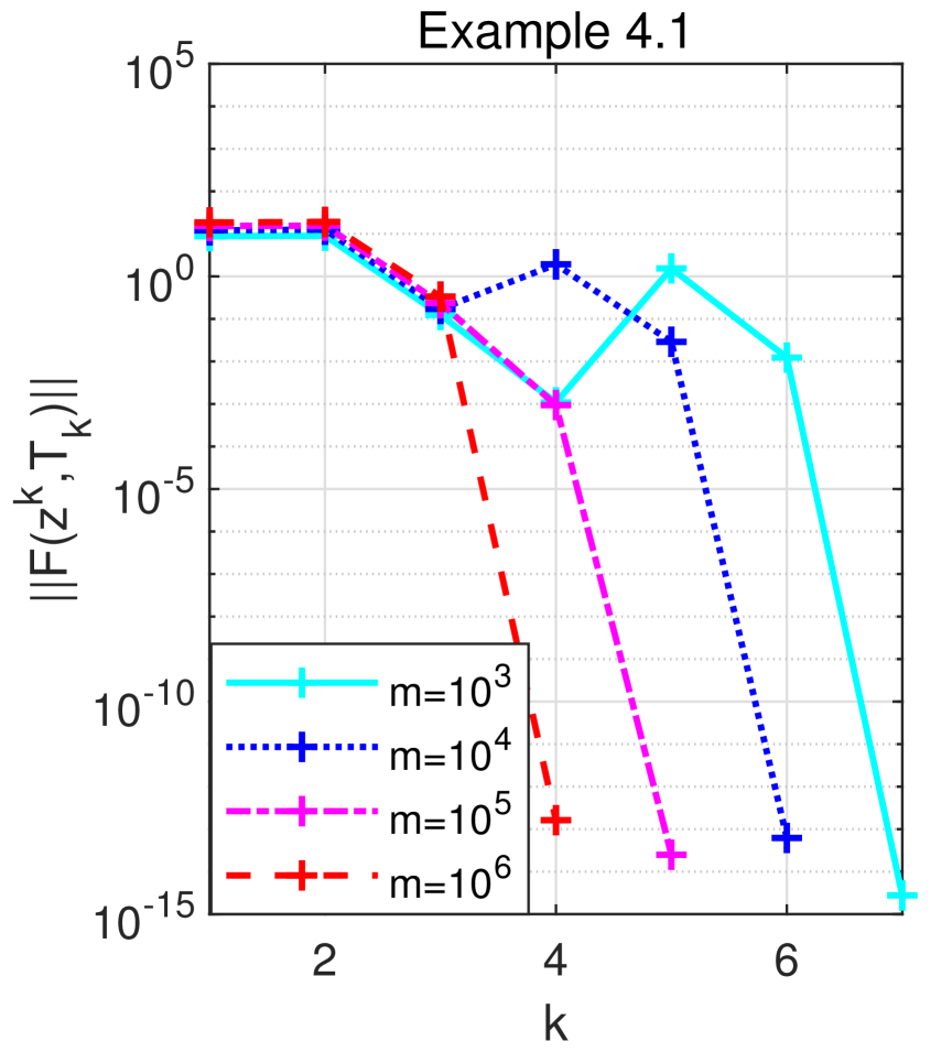
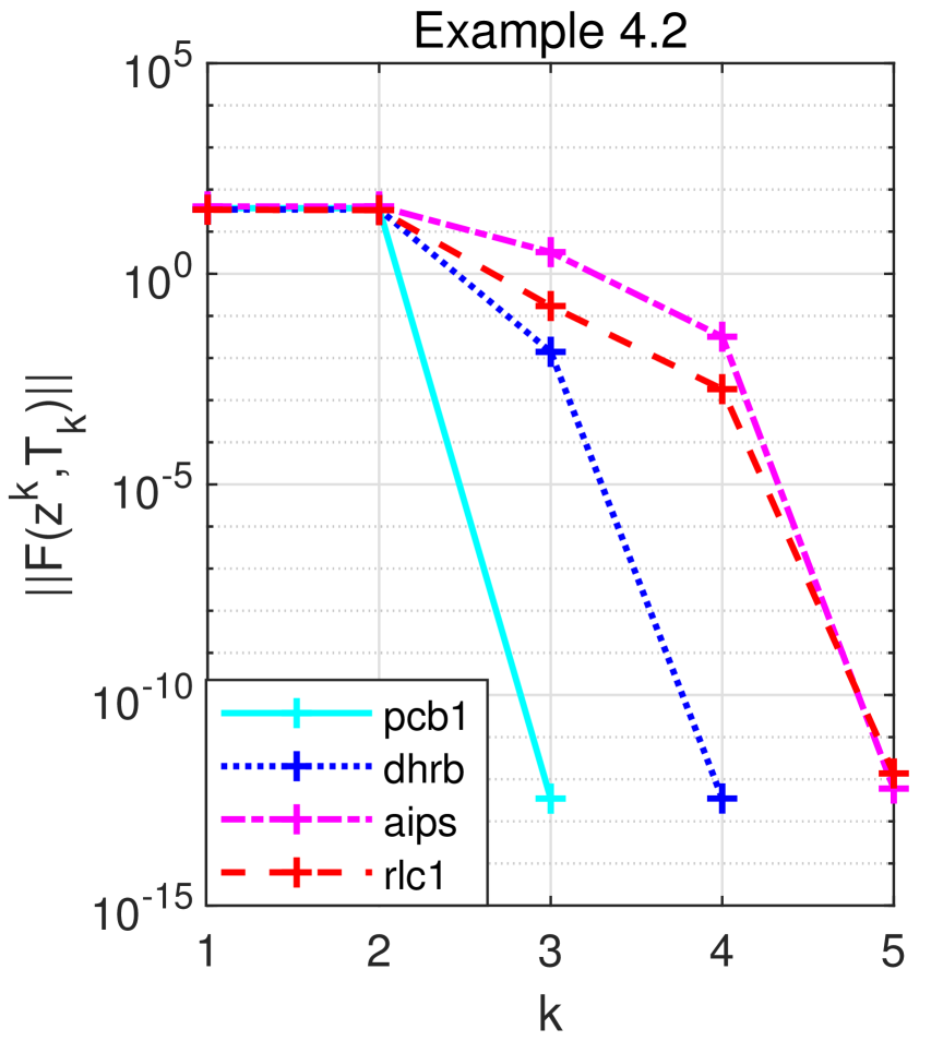
Figure 1: Decreasing of $\|F({\bf z}^{k},T_{k})\|$.

We note that Algorithm 1 can terminate at the next step if the current point falls into a local area of an $\eta$-stationary point. This means that if by chance the starting point is chosen within the local area, the proposed algorithm will take one step to terminate. Hence, it enjoys a fast convergence property. Of course, this depends on the choices of the initial point. In reality, how close the initial point is to an $\eta$-stationary point is unknown. Nevertheless, numerical experiments show that the proposed method is insensitive the choice of the starting point. It can take a few steps to converge. For instance, the results of Algorithm 1 solving Example 4.1 and Example 4.2 with the initial point ${\bf{\bm{\alpha}}}^{0}=0$ and $b^{0}={\rm sgn}(\langle{\bf y},{\bf 1}\rangle)$ were presented in Fig. 1. The line of pcb1 showed that the point ${\bf z}^{3}$ at step 3 may fall into a local area of an $\eta$-stationary point since $\|F({\bf z}^{4},T_{4})\|(\approx 10^{-12})$ almost reached 0 at step 4. Therefore, it terminated at step 4. This showed potential of termination at the next step, even though the initial point was not close to the $\eta$-stationary point. Similar observations can be found for all other lines.

Moreover, Theorem 2.4 states that the $\eta$-stationary point is a local minimizer of the problem (8). Hence, Algorithm 1 at least converges to a local minimizer. If further $\|{\bf z}^{*}\|_{0}<s$ or $\|{\bf z}^{*}\|_{0}=s$ and $\eta^{*}\geq C$, then the $\eta$-stationary point is also a global minimizer by Theorem 2.4 c) and d), namely, Algorithm 1 converges to the global minimizer.

3.3 Sparsity Level Tuning

One major issue encountered in practice is that the sparsity level $s$ in (8) is usually unknown beforehand. The level has two important effects: (i) A larger $s$ corresponds to better classifications since more samples are taken into consideration. (ii) However, a smaller $s$ leads to higher computational speed of Algorithm 1 because the complexity in (64) depends on $s$. Moreover, according to (1) that the number of support vectors is smaller than $\|{\bf{\bm{\alpha}}}\|_{0}\leq s$, a smaller $s$ results in a smaller number of support vectors. Therefore, to balance these two requirements, we design the following rule to update the unknown $s$. We start with a small integer and then increase it until the following halting conditions are satisfied

$$\|F({\bf z}^{k};T_{k})\| < \epsilon,$$ (66)

$$\Big{|}{\tt ACC}({\bf{\bm{\alpha}}}^{k})-\max_{j\in[k-1]}{\tt ACC}({\bf{\bm{\alpha}}}^{j})\Big{|} < 10^{-4},$$ (67)

where we admit ${\tt ACC}({\bf{\bm{\alpha}}}^{-1})=0$ and ${\tt ACC}({\bf{\bm{\alpha}}})$ is defined by

$${\tt ACC}({\bf{\bm{\alpha}}}):=\left[1-\frac{1}{m}{\|{\rm sgn}(X{\bf{\bm{\alpha}}}+b)-{\bf y}\|_{0}}\right]\times 100\%,$$ (68)

with ${\rm sgn}(t)=1$ if $t>0$ and $-1$ otherwise. The halting condition (66) means that ${\bf{\bm{\alpha}}}^{k}$ is almost an $\eta$-stationary point due to the small $\|F({\bf z}^{k};T_{k})\|$, while (67) implies that the classification accuracy ${\tt ACC}({\bf{\bm{\alpha}}}^{k})$ does not increase significantly. Therefore, it is unreasonable to further increase $s$ to achieve a better solution because a larger $s$ will lead to greater computational cost. Our numerical experiments demonstrate that Algorithm 1 under this scheme works very well. Overall, we derive NSSVM in Algorithm 2.

Algorithm 2 NSSVM: Newton method for sparse SVM with adaptively tuning the sparsity level $s$.

  Give parameters $C>c,\eta,\epsilon,K>0,\sigma>1,s_{0}\in[m]$.

  Initialize ${\bf z}^{0}$, pick $T_{0}\in{\mathbb{T}}_{s_{0}}({\bf{\bm{\alpha}}}^{0}-\eta g({\bf z}^{0}))$ and set $k:=0$.

  while ${\bf z}^{k}$ violates (66) and (67) and $k\leq$MaxIt do

      Update ${\bf d}^{k}$ by solving (52).

      Update ${\bf z}^{k+1}$ by (62).

      Update $s_{k+1}=\sigma s_{k}$ if $k$ is a multiple of $10$ or (66) is met, and $s_{k+1}=s_{k}$ otherwise.

      Update $T_{k+1}\in{\mathbb{T}}_{s_{k+1}}({\bf{\bm{\alpha}}}^{k+1}-\eta g({\bf z}^{k+1}))$ and $k:=k+1$.

  end while

  return  the solution ${\bf z}^{k}$.

4 Numerical Experiments

This part conducts extensive numerical experiments of Algorithm 1 and Algorithm 2 (NSSVM) by using MATLAB (R2019a) on a laptop with $32$GB memory and Inter(R) Core(TM) i9-9880H 2.3Ghz CPU.

4.1 Testing Examples

We first consider a two-dimensional example with synthetic data, where the features come from Gaussian distributions.

Example 4.1 (Synthetic data in ${\mathbb{R}}^{2}$ [6, 42])

Samples ${\bf x}_{i}$ with positive labels $y_{i}=+1$ are drawn from the normal distribution with mean $(0.5,-3)^{\top}$ and variance $\Sigma$, and samples ${\bf x}_{j}$ with negative labels $y_{j}=-1$ are drawn from the normal distribution with mean $(-0.5,3)^{\top}$ and variance $\Lambda$, where $\Sigma$ and $\Lambda$ are diagonal matrices with $\Sigma_{11}=\Lambda_{11}=0.2,~{}\Sigma_{22}=\Lambda_{22}=3.$ We generate $2m$ samples with equal numbers of two classes and then evenly split them into a training and a testing set.

Example 4.2 (Real data in higher dimensions)

We select 30 datasets with $m\gg n$ from the libraries: libsvm, uci and kiggle. Here, $aeb:=a\times 10^{b}$. All datasets are feature-wisely scaled to $[-1,1]$ and all of the classes that are not $1$ are treated as $-1$. Their details are presented in Table III, where $7$ datasets have the testing data. For each of the dataset without the testing data, we split the dataset into two parts. The first part contains 90% of samples treated as the training data and the rest are the testing data.

TABLE III: Descriptions of real datasets.

Data	Datasets	Source		Train	Test
			$n$	$m$	$m_{t}$
pcb1	Polish companies bankruptcy data	uci	64	7027	0
pcb2		uci	64	10173	0
pcb3		uci	64	10503	0
pcb4		uci	64	9792	0
pcb5		uci	64	5910	0
a5a	A5a	libsvm	123	6414	26147
a6a	A6a	libsvm	123	11220	21341
a7a	A7a	libsvm	123	16100	16461
a8a	A8a	libsvm	123	22696	9865
a9a	A9a	libsvm	123	32561	16281
mrpe	malware analysis datasets	kaggle	1024	51959	0
dhrb	hospital readmissions bnary	kaggle	17	59557	0
aips	airline passenger satisfaction	kaggle	22	103904	25976
sctp	santander customer transaction	kaggle	200	200000	0
skin	skin_nonskin	libsvm	3	245056	0
ccfd	credit card fraud dtection	kaggle	28	284807	0
rlc1	record linkage comparison patterns	uci	9	574914	0
$\cdots$		$\cdots$	$\cdots$	$\cdots$	$\cdots$
rlc10		uci	9	574914	0
covt	covtype.binary	libsvm	54	581012	0
susy	susy	uci	18	$5e6$	0
hepm	hepmass	uci	28	$7e6$	$35e5$
higg	higgs	uci	28	$11e6$	0

To compare the performance of all selected methods, let ${\bf{\bm{\alpha}}}$ be the solution/classifier generated by one method. We report the CPU time (TIME), the training classification accuracy (ACC) by (68) where $X$ and ${\bf y}$ are the training samples and classes, the testing classification accuracy (TACC) by (68) where $X$ and ${\bf y}$ are the testing samples and classes, and the number of support vectors (NSV).

4.2 Implementation and parameters tuning

The starting point ${\bf z}^{0}$ is initialized as ${\bf{\bm{\alpha}}}^{0}=0$ and $b^{0}={\rm sgn}(\langle{\bf y},{\bf 1}\rangle)$ if no additional information is provided. The maximum number of iterations and the tolerance are set as $K=1000$, $\epsilon=\max\{\sqrt{m}$ and $\sqrt{n}\}10^{-6}$. Recall that the model (8) involves three important parameters $C,c$ and $s$ and the $\eta$-stationary point has the parameter $\eta$. We now apply Algorithm 1 for tuning them as described below.

4.2.1 Effect of $\eta$

For Example 4.1, we fix $C=2^{-2},c=C/2,s=0.005m$ and vary $\eta\in[10^{-8},10^{-2}]$ and $m\in\{2,4,6,8\}\times 10^{4}$ to examine the effect of $\eta$ on Algorithm 1. For each case $(m,\eta)$, we run 100 trials and report the average results in Fig. 2. It is clearly observed that the method was insensitive to $\eta$ in the range $[10^{-8},10^{-6}]$. For each $m$, the ACC lines were stabilized at a certain level when $\eta\in[10^{-8},10^{-6}]$, increased when $\eta\in[10^{-6},10^{-4}]$ and then decreased. It appears that $\eta$ of approximately $10^{-4}$ gave the best performance for Algorithm 1 in terms of the highest ACC. Moreover, we tested problems with different dimensions and found that $\eta=1/m$ enabled the algorithm to achieve steady behaviour. Therefore, we set this option for $\eta$ in the subsequent numerical experiments if no additional information is provided.

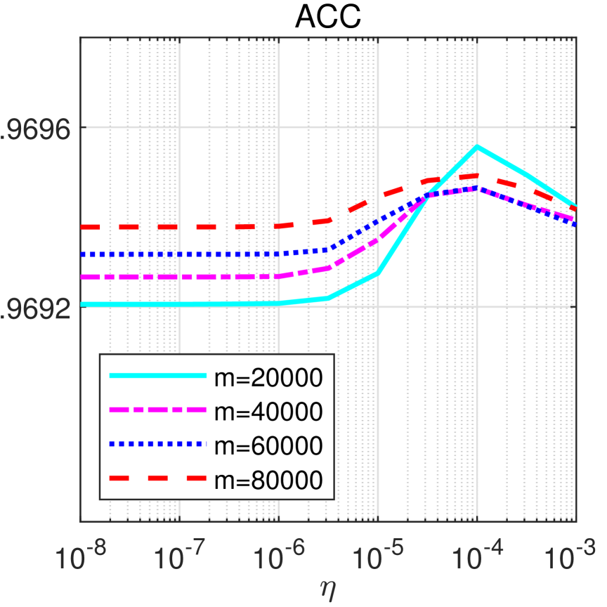
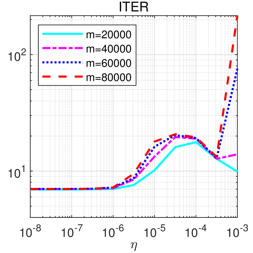
Figure 2: Effect of $\eta$.

4.2.2 Effect of $C$ and $c$

To see the effect of parameters $C$ and $c$, we choose $C\in\{2^{-3},2^{-2},2^{-1},2^{0},2^{1}\}$ and $c=aC$, where $a\in[0.001,1]$. Again, we apply Algorithm 1 for solving Example 4.1 with fixing $m=10000$ and $s=0.005m$. The average results were recoded in Fig. 3, where it was observed that ACC reached the highest peak at $a=c/C=0.01$. When $c/C\geq 0.02$, the bigger $C$ was, the higher ACC was but the larger ITER was as well. To balance the accuracy and the number of iterations, in the following numerical experiments, we set $C=0.25$ and $c=0.01C$ unless specified otherwise.

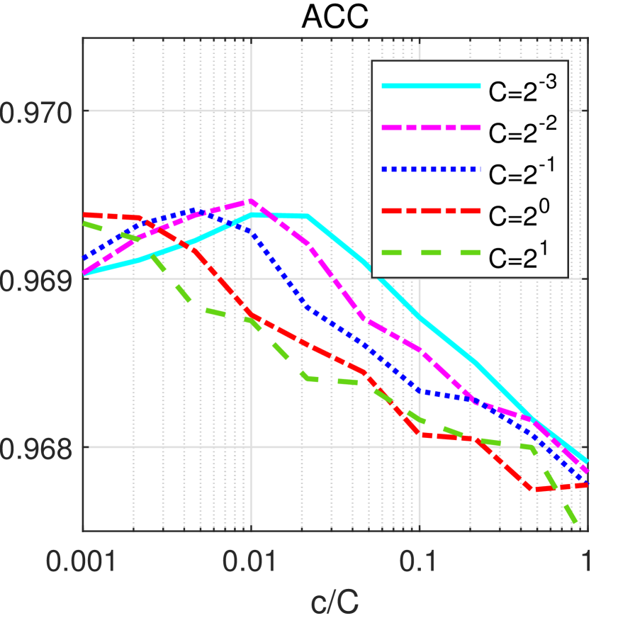
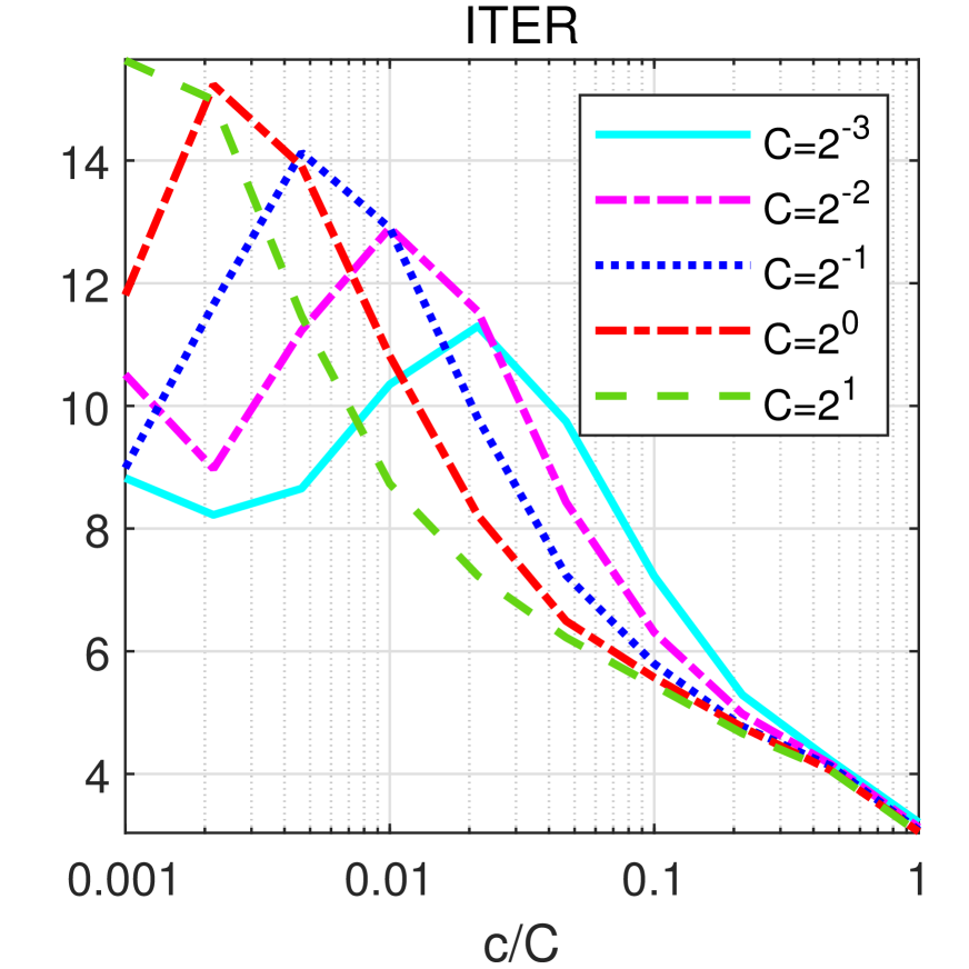
Figure 3: Effect of $C$ and $c$.

4.2.3 Effect of $s$

Apparently, the sparsity level $s$ has a strong influence on the solutions to the problem (8) and impacts the computational complexity of Algorithm 1. Below, we use the following rule to tune the sparsity level $s$,

$$s(\beta):=\lceil\beta n({\rm log}_{2}(m/n))^{2}\rceil,$$

where $\lceil t\rceil$ presents the smallest integer that is no less than $t$, and $\beta$ is chosen based on the problem to be solved. We use this rule because it relies on the dimensions of a given problem and allows Algorithm 1 to deliver an overall desirable performance. By setting $s=s(\beta)$, we focus on selecting a proper $\beta$. We note that $s$ increases with the rising of $\beta$. As demonstrated in Fig. 4, where Example 4.1 was solved again, the average results showed the effect of $\beta\in[0.1,1]$ (i.e., the effect of $s$) of the algorithm. It is observed from the figure that ACC increased with increasing $s$ but gradually stabilized at a certain level after $\beta>0.4$, indicating that there was no need to increase $s$ beyond this point. Furthermore, the small number of iterations showed that Algorithm 1 can converge quickly.

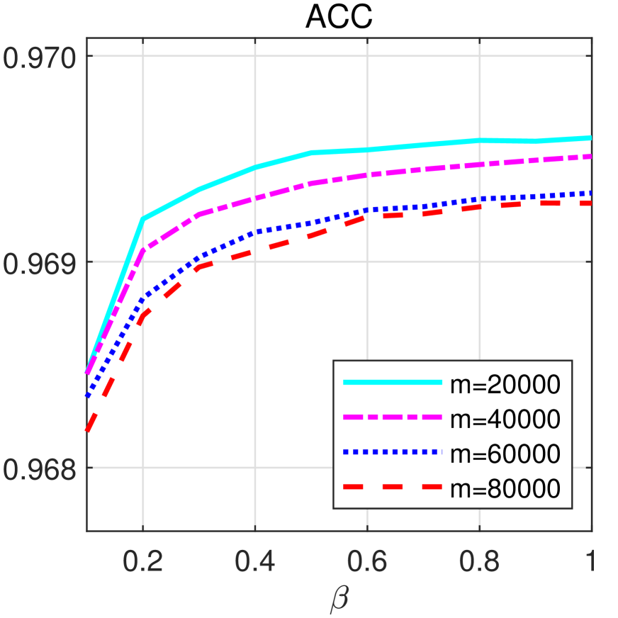
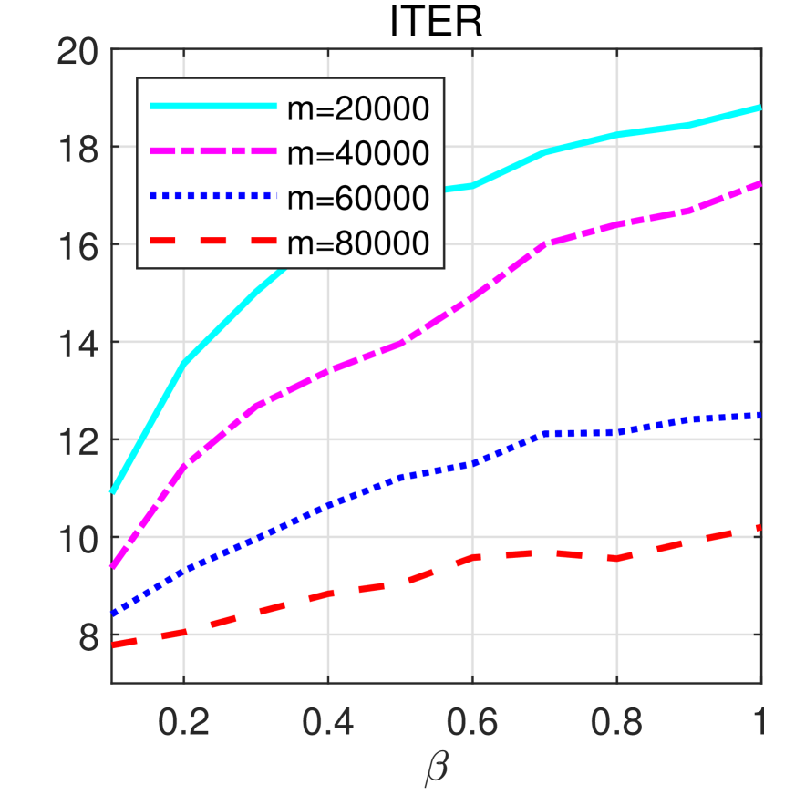
Figure 4: Effect of $s$.

4.2.4 Effect of the initial points

Theorem 3.1 states that the algorithm can converge at the next step if the initial point is sufficiently close to an $\eta$-stationary point that however is unknown beforehand. Therefore, we examine how the initial points affect the performance of Algorithm 1. To carry out this study, we apply the algorithm for solving Example 4.1 with $m=10^{6}$ and $s=s(1)$, and Example 4.2 with datasets: rcl1, rcl2, rcl3 and $s=s(0.05)$. For each data, we run the algorithm under $50$ different initial points ${\bf{\bm{\alpha}}}^{0}$. The first point is ${\bf{\bm{\alpha}}}^{0}=0$ and the other $49$ points have randomly generated entries from the uniform distribution, namely, $\alpha_{i}^{0}\sim U[0,1]$. The results were plotted in Fig. 5, where the x-axis represents the 50 initial points. For each dataset, all ACC stabilized at a certain level, indicating that these initial points had little effect on the accuracy. The results for ${\tt ITER}$ illustrated that the algorithm converged very quickly, stopping within $6$ steps for all cases. To summarize, Algorithm 1 was not too sensitive to the choice of the initial point for these datasets. Hence, for simplicity, we initialize our algorithm with ${\bf{\bm{\alpha}}}^{0}=0$ and $b^{0}={\rm sgn}(\langle{\bf y},{\bf 1}\rangle)$ in the sequel.

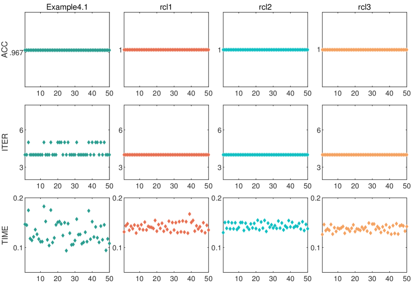
Figure 5: Robust to the initial points ${\bf{\bm{\alpha}}}^{0}$.

4.3 Algorithm 1 v.s. Algorithm 2: NSSVM

We now turn our attention to NSSVM in Algorithm 2. It reduces to Algorithm 1 if we set $\sigma=1$, namely, $s_{k}=s_{0}$ remains invariant. However, to distinguish them, in the following, we always set $\sigma=1.1$. In this subsection, we focus on how the sparsity level tuning strategy in NSSVM affects the final results. For Algorithm 1, we implement it with different fixed $si=s(\beta_{i}),i=1,2,3$ and name it Alg1-si. In particular, we use $\beta_{1}=0.4,\beta_{2}=0.5,\beta_{3}=0.8$. Recall that NSSVM also requires an initial sparsity level $s_{0}$ that is set as $s_{0}=s(0.4)=s1$. Therefore, NSSVM and Alg1-s1 start with the same initial sparsity level.

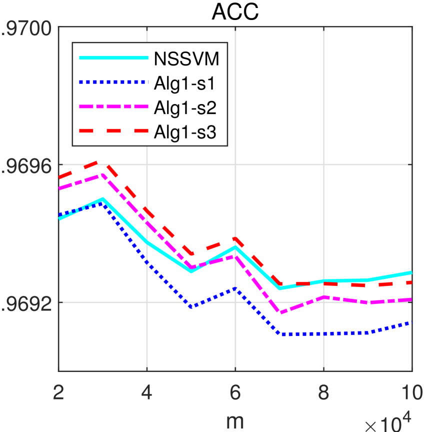
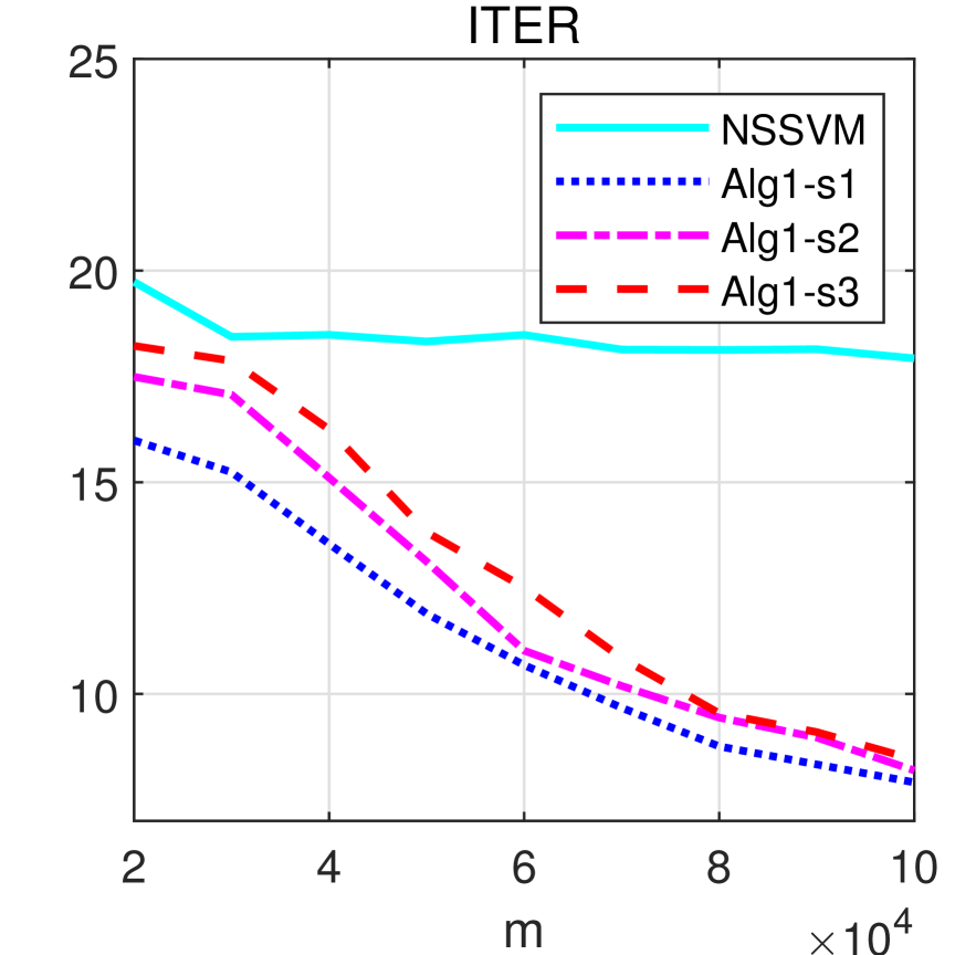
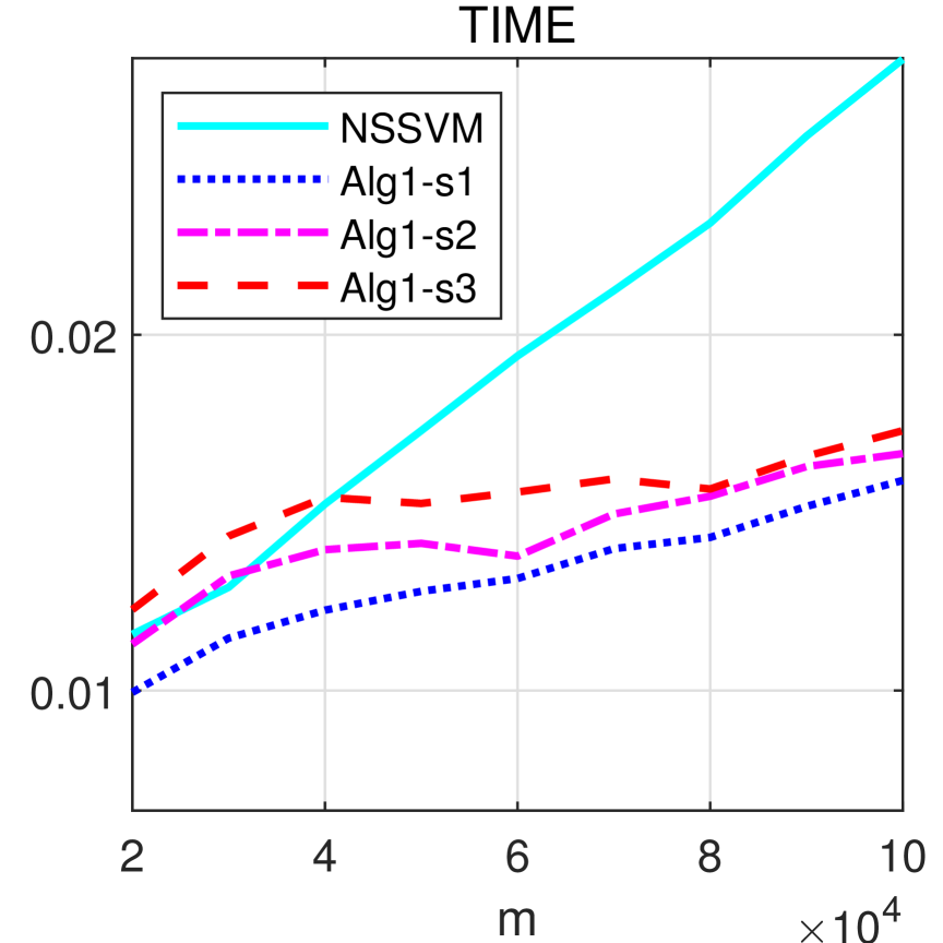
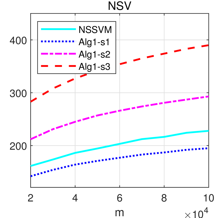
Figure 6: Algorithm 1 v.s. Algorithm 2

The average results of two algorithms used to solve Example 4.1 were displayed in Fig. 6. First, despite starting with the same initial sparsity level, NSSVM generated higher ACC than Alg1-s1 because it used more support vectors (i.e., higher NSV) due to the tuning strategy. Second, NSSVM obtained higher ACC than that produced by Alg1-s2 and Alg1-s3 when $m\geq 70000$, but yielded much lower NSV. This indicated that the tuning strategy performed well to find a proper sparsity level to maximize the accuracy. Clearly, NSSVM required longer time because the tuning strategy led to more steps to meet the stopping criteria (66). Nevertheless, NSSVM still ran quickly, requiring less than 0.03 second and 20 steps to converge.

We also compared Algorithm 1 and NSSVM for solving the real datasets, and omitted similar observations. In a nutshell, the tuning strategy enables NSSVM to deliver higher accuracy with slightly longer computational time. Based on this, we next conduct some numerical comparisons between NSSVM and some state-of-the-art solvers.

4.4 Numerical Comparisons

We note that NSSVM involves four parameters $(\eta,C,c,s0)$. On the one hand, it is impractical to derive a universal combination of these four parameters for all datasets. On the other hand, tuning them for each dataset will increase the computational cost. Therefore, in the following numerical experiments, we seek to avoid using different parameters for different datasets. Typically, we fix $\eta=1/m$ and $c=0.01C$, but select $C$ and $s_{0}$ as specified in Table IV.

TABLE IV: Selection of parameters.

	cases	$C$	$s_{0}$
Example 4.1	$m\leq 10^{4}$	0.25	$s(0.5)$
	$m>10^{4}$	0.25	$s(1)$
	higg, susy, covt, hemp	$\log_{2}(m)$	$s(10)$
Example 4.2	a5a-a9a	$0.25$	$s(0.2)$
	other	$0.25$	$s(0.05)$

4.4.1 Benchmark methods

There is an impressive body of work that has developed numerical methods to tackle the SVM, such as those in [47, 43, 45, 44, 46]. They perform very well, especially for datasets in small or mediate size. Unfortunately, it is unlikely to find a MATLAB implementation for sparse SVM on which we could successfully perform the experiments. For instance, the methods in [45] for RSVM [20] and the one in [24] were programmed by C++ and couldn’t run by MATLAB.

TABLE V: Benchmark methods.

Algs.	Source of Code	Ref.	$\ell$
HSVM	libsvm	[47]	Hinge loss
SSVM	liblssvm	[43]	Squared Hinge loss
LSVM	liblinear	[48]	Hinge loss
FSVM	fitclinear		Hinge loss
SNSVM	Li’s lab	[46]	Squared Hinge loss

Therefore, we select five solvers in Table V that do not aim at the sparse SVM. They address the soft-margin SVM models (2) with different loss functions $\ell$. Note that fitclinear is a Matlab built-in solver with initializing Solver = ‘dual’ in order to obtain the number of the support vectors. For the same reason, we set -s 3 for FSVM. It runs much faster if we set -s 2, but such a setting does not offer the number of support vectors. The other three methods also involve some parameters. For simplicity, all of these parameters are set to their default values.

4.4.2 Comparisons for datasets with small sizes

We first applied five solvers for solving Example 4.1 with small scales $m=200,400$ and depicted the classifiers in Fig. 7 where the Bayes classifier was $w_{2}=0.25w_{1}$, see the black dotted line. We did not run HSVM because it solved the dual problem and did not provide the solution $({\bf w},b)$. Overall, all solvers can classify the dataset well.

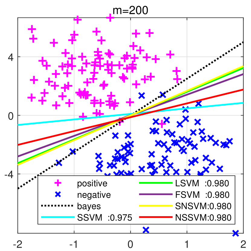
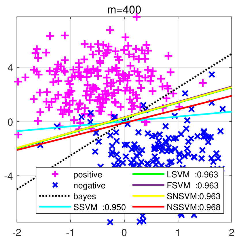
Figure 7: Classifiers by five solvers for Example 4.1.

We then used six solvers to address Example 4.1 with different sample sizes $m\in[2000,10^{4}]$. Average results over 100 trials were reported in Fig. 8. It is observed that NSSVM obtained the largest ACC, but rendered smallest TACC for most cases. This was probably due to the smallest number of support vectors used. Evidently, LSVM and SNSVM ran the fastest, followed by FSVM and NSSVM.

Next, six methods were used to handle Example 4.2 with small scale datasets. As shown in Table VI, where ‘$--$’ denoted that SSVM required memory that was beyond the capacity of our laptop; here, again NSSVM did not show the advantage of delivering the accuracy. This was not surprising because it used a relatively small number of support vectors. However, it ran the fastest for most datasets.

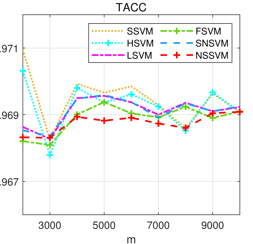
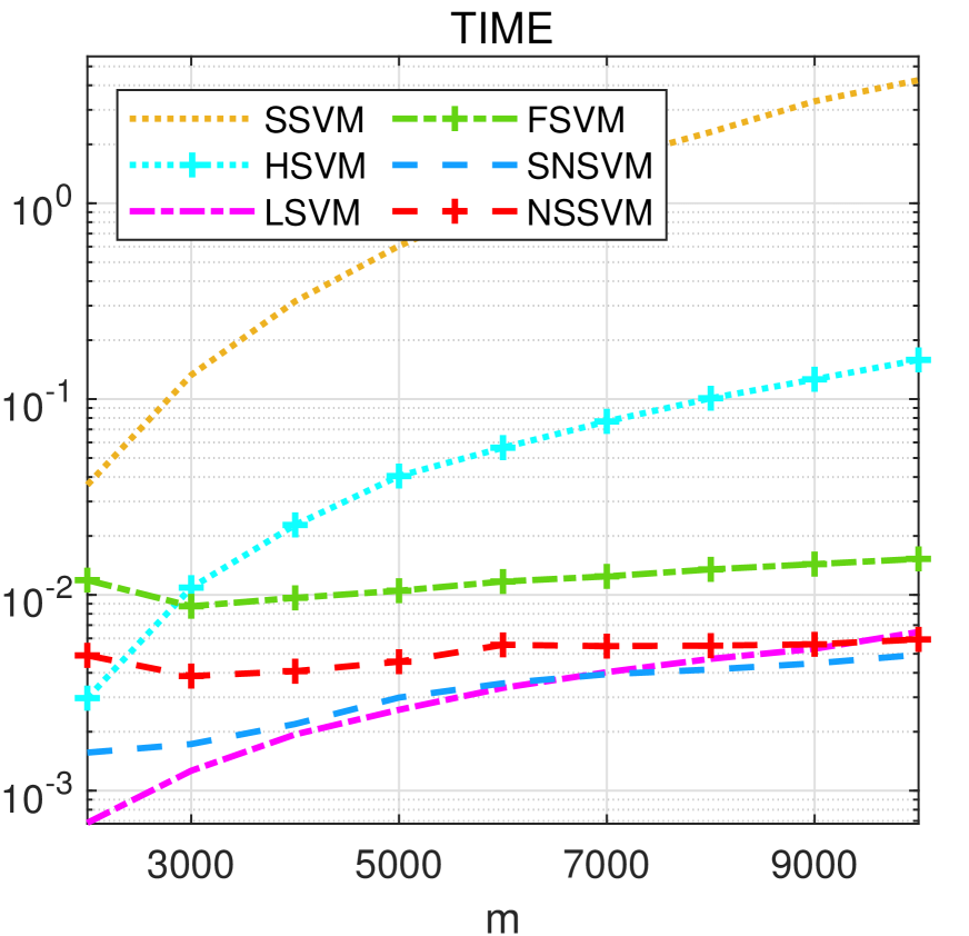
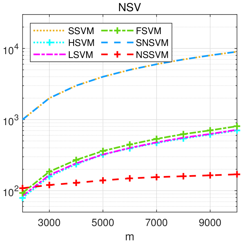
Figure 8: Average results of six solvers for Example 4.1.

To summarize, NSSVM did not present the advantage of higher accuracy for dealing with small scale datasets. One reason for this is that the solution to the model (8) may not be sufficiently sparse for small scale datasets. In other words, there is no strong need to perform data reduction for these datasets. Hence, in the sequel, we employ four methods to address test problems with datasets on much larger scales. However, we remove HSVM and SSVM from comparisons in the following since they either are too slow or required memory beyond the capability of our device.

TABLE VI: Results of six solvers solving Example 4.2 with datasets with small sizes.

	SSVM	HSVM	LSVM	FSVM	SNSVM	NSSVM
	ACC (%)
pcb1	96.21	96.22	96.22	96.22	96.24	96.24
pcb2	95.95	95.96	95.96	95.96	95.97	95.95
pcb3	95.31	95.31	95.31	95.31	95.30	95.31
pcb4	94.71	94.74	94.74	94.74	94.72	94.71
pcb5	93.04	93.12	93.16	93.16	93.18	93.04
a5a	24.46	85.06	85.05	81.82	85.16	84.10
a6a	$--$	84.89	84.87	76.11	84.80	83.95
a7a	$--$	84.88	84.96	81.93	84.89	84.16
a8a	$--$	84.69	84.67	83.00	84.74	84.01
a9a	$--$	84.99	84.99	80.63	84.96	84.04
	TACC (%)
pcb	95.73	95.58	95.58	95.58	95.58	95.58
pcb2	96.85	97.15	97.15	97.15	97.15	97.15
pcb3	95.05	95.05	95.05	95.05	95.05	95.05
pcb4	94.69	94.99	94.99	94.99	94.89	94.99
pcb5	93.06	93.23	93.23	93.23	93.23	93.23
a5a	84.42	84.39	84.39	81.07	84.50	83.60
a6a	$--$	84.72	84.66	76.12	84.77	84.13
a7a	$--$	84.84	84.82	82.26	85.00	84.00
a8a	$--$	85.16	85.13	83.47	85.42	84.59
a9a	$--$	84.98	85.00	80.96	84.94	84.47
	TIME (in seconds)
pcb1	1.905	0.702	0.037	0.241	0.057	0.082
pcb2	4.656	1.577	0.051	0.243	0.064	0.039
pcb3	4.987	1.761	0.046	0.064	0.044	0.019
pcb4	4.282	1.722	0.048	0.051	0.038	0.016
pcb5	1.241	0.805	0.044	0.033	0.021	0.013
a5	29.72	5.414	0.030	0.110	0.044	0.049
a6a	$--$	11.15	0.051	0.247	0.107	0.085
a7a	$--$	19.15	0.067	0.072	0.179	0.097
a8a	$--$	33.07	0.105	0.067	0.287	0.121
a9a	$--$	70.59	0.158	0.072	0.361	0.130
	NSV
pcb1	6325	497	2320	2263	6325	190
pcb2	9156	791	4166	3557	9156	182
pcb3	9453	981	4692	4375	9453	184
pcb4	8813	990	4538	4762	8813	179
pcb5	5319	758	2167	2440	5319	145
a5a	6414	2294	2332	3891	6414	882
a6a	$--$	4011	4082	6910	11220	1148
a7a	$--$	5757	5899	9931	16100	1339
a8a	$--$	8135	8292	13992	22696	1534
a9a	$--$	11533	11772	20030	32561	1754

4.4.3 Comparisons for datasets with large sizes

This part focus on instances with much larger scales. First, we employ four algorithms to solve Example 4.1 with $m$ from $[10^{5},10^{8}]$. The data reported in Table VII were the results averaged over 20 trials. Since LSVM ran for too long when $m>10^{6}$, its results were omitted. The training classification accuracy values for NSSVM, SNSVM and LSVM were similar and were better than those obtained by FSVM. However, it is clearly observed that NSSVM ran the fastest and used much fewer support vectors. Moreover, the superiority of NSSVM becomes more evident with larger $m$.

TABLE VII: Results of four solvers solving Example 4.1 with large-scale datasets.

$m$	LSVM	FSVM	SNSVM	NSSVM		LSVM	FSVM	SNSVM	NSSVM
	ACC (%)					TACC (%)
$10^{5}$	96.95	96.91	96.95	96.95		96.96	96.93	96.96	96.94
$10^{6}$	96.94	96.91	96.94	96.94		96.94	96.93	96.94	96.93
$10^{7}$	$--$	96.92	96.93	96.93		$--$	96.93	96.93	96.93
$10^{8}$	$--$	96.91	96.93	96.93		$--$	96.93	96.93	96.93
	TIME (in seconds)					NSV$/m$
$10^{5}$	0.10	0.10	0.04	0.04		7.83e-2	8.85e-2	1	5.94e-3
$10^{6}$	3.88	2.43	0.36	0.33		7.81e-2	8.87e-2	1	8.62e-4
$10^{7}$	$--$	30.62	3.42	2.08		$--$	8.88e-2	1	1.09e-4
$10^{8}$	$--$	447.1	34.1	12.3		$--$	8.89e-2	1	1.44e-5

TABLE VIII: Results of four solvers solving Example 4.2 with datasets with large sizes.

	LSVM	FSVM	SNSVM	NSSVM		LSVM	FSVM	SNSVM	NSSVM
	ACC (%)					TACC (%)
mrpe	95.01	94.78	95.08	95.00		95.25	94.90	95.25	95.25
dhrb	82.70	82.71	83.25	82.76		83.43	83.43	84.11	83.48
aips	87.66	87.26	87.42	86.54		87.41	87.08	87.13	85.99
sctp	89.95	78.01	91.20	90.50		90.00	77.80	91.19	90.51
skin	92.90	92.73	92.37	91.04		92.66	92.45	92.23	90.63
ccfd	99.94	99.94	99.92	99.94		99.92	99.92	99.88	99.92
rlc1	100.0	100.0	100.0	100.0		100.0	100.0	100.0	100.0
rlc2	100.0	100.0	100.0	100.0		100.0	100.0	100.0	100.0
rlc3	100.0	100.0	100.0	100.0		100.0	100.0	99.99	100.0
rlc4	100.0	100.0	100.0	100.0		100.0	100.0	100.0	100.0
rlc5	100.0	100.0	100.0	100.0		100.0	100.0	100.0	100.0
rlc6	100.0	100.0	100.0	100.0		100.0	100.0	99.99	99.99
rlc7	100.0	100.0	100.0	100.0		100.0	100.0	100.0	100.0
rlc8	100.0	100.0	100.0	100.0		100.0	100.0	100.0	100.0
rlc9	100.0	100.0	100.0	100.0		100.0	100.0	100.0	100.0
rlc10	100.0	100.0	100.0	100.0		100.0	100.0	100.0	100.0
covt	76.29	75.73	75.67	75.67		76.15	75.47	75.54	75.51
susy	78.44	78.55	78.66	78.82		78.39	78.52	78.63	78.79
hepm	78.36	83.31	83.63	83.74		78.33	83.23	83.61	83.71
higg	47.01	63.84	64.13	64.16		46.98	63.79	64.07	64.08
	TIME (in seconds)					NSV$/m$
mrpe	31.75	2.28	5.37	1.06		8.23e-1	5.60e-1	1	3.63e-2
dhrb	0.17	0.10	0.07	0.04		7.68e-1	6.92e-1	1	2.59e-3
aips	0.87	0.21	0.18	0.09		3.01e-1	5.30e-1	1	2.33e-3
sctp	13.48	1.09	10.61	0.38		3.82e-1	5.79e-1	1	5.84e-3
skin	0.42	0.33	0.11	0.08		1.97e-1	2.55e-1	1	2.20e-4
ccfd	2.66	0.52	0.40	0.16		5.56e-3	1.01e-2	1	9.41e-4
rlc1	0.39	0.66	0.25	0.11		3.32e-4	5.95e-4	1	2.17e-4
rlc2	0.39	0.51	0.26	0.17		2.47e-4	5.13e-4	1	2.40e-4
rlc3	0.49	0.56	0.23	0.12		2.85e-4	5.86e-4	1	2.17e-4
rlc4	0.38	0.67	0.25	0.18		2.68e-4	5.79e-4	1	2.40e-4
rlc5	0.40	0.57	0.26	0.12		2.89e-4	5.76e-4	1	2.17e-4
rlc6	0.50	0.51	0.27	0.21		2.44e-4	5.51e-4	1	2.64e-4
rlc7	0.38	0.52	0.25	0.12		2.84e-4	5.31e-4	1	2.17e-4
rlc8	0.68	0.67	0.25	0.12		2.68e-4	5.77e-4	1	2.17e-4
rlc9	0.66	0.54	0.25	0.12		3.04e-4	6.00e-4	1	2.17e-4
rlc10	0.39	0.55	0.25	0.12		3.25e-4	5.91e-4	1	2.17e-4
covt	13.23	2.05	9.22	1.11		4.75e-1	5.93e-1	1	1.61e-1
susy	596.3	16.69	16.44	2.43		4.15e-1	4.74e-1	1	1.26e-2
hepm	1688	28.39	26.97	3.62		3.45e-1	4.76e-1	1	1.27e-2
higg	2938	46.86	61.75	4.78		2.37e-1	7.30e-1	1	8.56e-3

Results obtained by four solvers for classifying real datasets in Example 4.2 on larger scales were reported in Table VIII. For the accuracy, there was no significant difference of ACC and TACC produced by four solvers. For the computational speed, it is clearly observed that NSSVM ran the fastest for all datasets. With regard to the number of support vectors, NSSVM outperformed the other methods because it obtained the smallest NSV. Taking higg as an instance, the other three solvers respectively produced $0.237m,0.73m$, and $m$ support vectors and consumed $2938$, $46.86$ and $61.75$ seconds to classify the data. By contrast, our proposed method used $0.00856m$ support vectors and only required $4.78$ seconds to achieve the highest classification accuracy.

In summary, NSSVM delivered the desirable classification accuracy and ran rapidly by using a relatively small number of support vectors for large-scale datasets.

5 Conclusion

The sparsity constraint was employed in the kernel-based SVM model (8) allowing for the control of the number of support vectors. Therefore, the memory required for data storage and the computational cost were significantly reduced, enabling large scale computation. We feel that the established theory and the proposed Newton type method deserve to be further explored for using the SVM model with some nonlinear kernel-based models.

Shenglong Zhou received the B.Sc. degree in information and computing science in 2011 and the M.Sc. degree in operational research in 2014 from Beijing Jiaotong University, China, and the Ph.D. degree in operational research in 2018 from the University of Southampton, the United Kingdom, where he was the Research Fellow from 2017 to 2019 and is currently a Teaching Fellow. His research interests include the theory and methods of optimization in the fields of sparse, low-rank matrix and bilevel optimization.

Appendix A Proofs of all theorems

Proof of Theorem 2.1

proof By introducing $u_{i}=1-y_{i}(\langle{\bf w},{\bf x}_{i}\rangle+b)$, the problem (4) is rewritten as

$$\min_{{\bf w},{\bf u}} \frac{1}{2}\|{\bf w}\|^{2}+\sum_{i=1}^{m}\ell_{cC}\left(u_{i}\right),$$ (69)

$${\rm s.t.} u_{i}+y_{i}(\langle{\bf w},{\bf x}_{i}\rangle+b)=1,~{}i\in[m].$$

The Lagrangian function of the above problem is

$$L({\bf w},{\bf u},b,{\bf{\bm{\alpha}}}) := \frac{1}{2}\|{\bf w}\|^{2}+\sum_{i=1}^{m}\ell_{cC}\left(u_{i}\right)$$

$$- \sum_{i=1}^{m}\alpha_{i}\Big{(}u_{i}+y_{i}(\langle{\bf w},{\bf x}_{i}\rangle+b)-1\Big{)}.$$

The dual problem of (69) is then given by

$$\max_{\bf{\bm{\alpha}}}\min_{{\bf w},{\bf u},b}L({\bf w},{\bf u},b,{\bf{\bm{\alpha}}}).$$ (70)

For a fixed ${\bf{\bm{\alpha}}}$, the inner problem $\min_{{\bf w},{\bf u},b}L({\bf w},{\bf u},b,{\bf{\bm{\alpha}}})$ has three variables that are independent of each other. Hence, it can be divided into three sub-problems

$$\min_{{\bf w},{\bf u},b}~{}~{}L({\bf w},{\bf u},b,{\bf{\bm{\alpha}}})$$

$$= \min_{{\bf w}}~{}\frac{1}{2}\|{\bf w}\|^{2}-\sum_{i=1}^{m}\alpha_{i}y_{i}\langle{\bf w},{\bf x}_{i}\rangle+\sum_{i=1}^{m}\alpha_{i}$$

$$+ \min_{{\bf u}}\sum_{i=1}^{m}\Big{(}\ell_{cC}(u_{i})-\alpha_{i}u_{i}\Big{)}-\underset{b}{\min}\sum_{i=1}^{m}\alpha_{i}y_{i}b.$$

For the sub-problem with respect to ${\bf w}$, the optimal solution ${\bf w}$ is attained at $w_{j}-\sum_{i=1}^{m}\alpha_{i}y_{i}x_{ij}=0,i\in[n]$, namely,

$${\bf w}=Q{\bf{\bm{\alpha}}}.$$ (72)

using notation $Q$ in Table I. Substituting (72) into the following objective function yields

$$\underset{{\bf w}}{\min}~{}\frac{1}{2}\|{\bf w}\|^{2}-\sum_{i=1}^{m}\alpha_{i}y_{i}\langle{\bf w},{\bf x}_{i}\rangle=-\frac{1}{2}\|Q{\bf{\bm{\alpha}}}\|^{2}.$$ (73)

For the sub-problem with respect to ${\bf u}$, the optimal solution ${\bf u}$ is attained at, for $i\in[m]$,

$$0=\ell^{\prime}_{c,C}(u_{i})-\alpha_{i}~{}~{}\Longleftrightarrow~{}~{}\alpha_{i}=\left\{\begin{array}[]{rr}Cu_{i},&u_{i}\geq 0,\\ cu_{i},&u_{i}<0,\end{array}\right.$$ (76)

where $\ell^{\prime}_{c,C}(u_{i})$ is the derivative of $\ell^{\prime}_{c,C}$ at $u_{i}$ that leads to

$$\ell_{cC}(u_{i})-\alpha_{i}u_{i} = \begin{cases}{C}u_{i}^{2}/2-\alpha_{i}u_{i},&u_{i}\geq 0,\\ {c}u_{i}^{2}/2-\alpha_{i}u_{i},&u_{i}<0,\end{cases}$$

$$= \begin{cases}-{\alpha_{i}^{2}}/{(2C)},&\alpha_{i}\geq 0,\\ -{\alpha_{i}^{2}}/{(2c)},&\alpha_{i}<0,\\ \end{cases}$$

$$= -h_{cC}(\alpha_{i}).$$

Therefore, we have the sub-problem

$$\underset{{\bf u}}{\min}~{}\sum_{i=1}^{m}\Big{(}\ell_{cC}(u_{i})-\alpha_{i}u_{i}\Big{)}=-\sum_{i=1}^{m}h_{cC}(\alpha_{i}).$$ (77)

For the third sub-problem with respect to $b$, the optimal solution is attained at

$$\langle{\bf{\bm{\alpha}}},{\bf y}\rangle=\sum_{i=1}^{m}\alpha_{i}y_{i}=0.$$ (78)

This results in

$${\min}_{b}\sum_{i=1}^{m}\alpha_{i}y_{i}b=0.$$

Overall, the sub-problem (A) becomes

$$\min_{{\bf w},{\bf u},b}~{}L({\bf w},{\bf u},b,{\bf{\bm{\alpha}}})=-\frac{1}{2}\|Q{\bf{\bm{\alpha}}}\|^{2}+\sum_{i=1}^{m}\alpha_{i}-h_{cC}(\alpha_{i})$$ (79)

where ${\bf{\bm{\alpha}}}$ satisfies (78). Hence, the dual problem (70) is equivalent to

$$\min_{\bf{\bm{\alpha}}}\Big{\{}-\min_{{\bf w},{\bf u},b}L({\bf w},{\bf u},b,{\bf{\bm{\alpha}}})\Big{\}}$$

$$= \min_{\bf{\bm{\alpha}}}\left\{\frac{1}{2}\|Q{\bf{\bm{\alpha}}}\|^{2}-\sum_{i=1}^{m}\alpha_{i}+h_{cC}(\alpha_{i}):\langle{\bf{\bm{\alpha}}},{\bf y}\rangle=0\right\},$$

which is same as (6). Let $(\widehat{\bf w},\widehat{\bf u},\widehat{b})$ and ${\bf{\bm{\alpha}}}^{*}$ be the optimal solutions to the primal problem (69) and dual problem (A), respectively. Then from (72), $\widehat{\bf w}=Q{\bf{\bm{\alpha}}}^{*}$. For $\widehat{b}$, it follows

$$y_{i}\widehat{b} \overset{\eqref{SM-SVM-h-equ}}{=} 1-\widehat{u}_{i}-\langle\widehat{\bf w},y_{i}{\bf x}_{i}\rangle$$

$$\overset{\eqref{SM-SVM-h-equ-dual-sub1-opt}}{=} 1-\widehat{u}_{i}-\langle Q{\bf{\bm{\alpha}}}^{*},y_{i}{\bf x}_{i}\rangle$$

$$\overset{\eqref{SM-SVM-h-equ-dual-sub2-opt},\eqref{diag-hessian}}{=} 1-E_{ii}({\bf{\bm{\alpha}}}^{*})\alpha_{i}^{*}-\langle Q{\bf{\bm{\alpha}}}^{*},y_{i}{\bf x}_{i}\rangle,$$

$$\overset{\eqref{SM-SVM-h-equ-dual-sparse-opt}}{=} 1-E_{iS_{*}}({\bf{\bm{\alpha}}}^{*})\alpha_{S_{*}}^{*}-\langle Q_{S_{*}}{\bf{\bm{\alpha}}}^{*}_{S_{*}},Q_{i}\rangle,$$

$$\overset{\eqref{gradient-hessian}}{=} 1-H_{iS_{*}}({\bf{\bm{\alpha}}}^{*})\alpha_{S_{*}}^{*},$$

for any $i\in S_{*}={\rm supp}({\bf{\bm{\alpha}}}^{*})$. This leads to

$$\widehat{b}=y_{i}-y_{i}H_{iS_{*}}({\bf{\bm{\alpha}}}^{*})\alpha_{S_{*}}^{*},\forall~{}i\in S_{*}.$$

Summing both sides of the above equation for all $i\in S_{*}$ yields $\widehat{b}$ in (23), completing the proof. $\Box$

Proof of Theorem 2.2

proof The solution set is nonempty since $0$ satisfies the constraints of (8). The problem can be written as

$$\min_{|T|\leq s,T\subseteq[m]}\Big{\{}\min_{{\bf{\bm{\alpha}}}\in{\mathbb{R}}^{m}}D(\alpha):\langle{\bf{\bm{\alpha}}}_{T},{\bf y}_{T}\rangle=0\Big{\}}.$$ (81)

It follows from (15) that $D(\cdot)$ is strongly convex. Therefore, the inner problem is a strongly convex program that admits a unique solution, say $\alpha_{T}$. In addition, the choices of $T$ such that $|T|\leq s,T\subseteq[m]$ are finitely many. To derive the global optimal solution, we pick one $T$ from the choices making $D(\alpha_{T})$ the smallest. $\Box$

Proof of Theorem 2.3

proof It follows from ${\bf z}^{*}$ being an $\eta$-stationary point and (32) that $\langle{\bf{\bm{\alpha}}}^{*},{\bf y}\rangle=0$ and

$${\bf{\bm{\alpha}}}^{*} \in {\mathbb{P}}_{s}\left({\bf{\bm{\alpha}}}^{*}-\eta g({\bf z}^{*})\right)$$

$$\overset{\eqref{P-s-T}}{=} \left\{\left[\begin{array}[]{c}{\bf{\bm{\alpha}}}^{*}_{T}-\eta g_{T}({\bf z}^{*})\\ 0\end{array}\right]:T\in{\mathbb{T}}_{s}({\bf{\bm{\alpha}}}^{*}-\eta g({\bf z}^{*}))\right\},$$

which is equivalent to stating that there exists a $T_{*}\in{\mathbb{T}}_{s}({\bf{\bm{\alpha}}}^{*}-\eta g({\bf z}^{*}))$ satisfying ${\bf{\bm{\alpha}}}_{\overline{T}_{*}}^{*}=0$ and $0=g_{T_{*}}({\bf z}^{*}).$ This can reach the conclusion immediately. $\Box$

A Lemma for Theorem 2.4

To prove Theorem 2.4, we need the following Lemma.

Lemma A.1

Consider a feasible point ${\bf{\bm{\alpha}}}^{*}$ to the problem (8), namely, $\|{\bf{\bm{\alpha}}}^{*}\|_{0}\leq s$ and $\langle{\bf{\bm{\alpha}}}^{*},{\bf y}\rangle=0$.

• It is a local minimizer if and only if there is $b^{*}\in{\mathbb{R}}$ such that

  $$\left\{\begin{array}[]{rll}g_{S_{*}}({\bf z}^{*})&=&0,\\ \langle{\bf{\bm{\alpha}}}^{*},{\bf y}\rangle&=&0,\\ \|{\bf{\bm{\alpha}}}^{*}\|_{0}&=&s,\end{array}\right.~{}~{}{\rm or}~{}~{}\left\{\begin{array}[]{rll}g({\bf z}^{*})&=&0,\\ \langle{\bf{\bm{\alpha}}}^{*},{\bf y}\rangle&=&0,\\ \|{\bf{\bm{\alpha}}}^{*}\|_{0}&<&s.\end{array}\right.$$ (89)

• If $\|{\bf{\bm{\alpha}}}^{*}\|_{0}<s$, then the local minimizer and the global minimizer are identical to each other and unique.

proof We only prove that the global minimizer ${\bf{\bm{\alpha}}}^{*}$ is unique if $\|{\bf{\bm{\alpha}}}^{*}\|_{0}<s$. The proofs of the remaining parts can be seen in [49, Theorem 3.2]. The condition in (15) indicates $D({\bf{\bm{\alpha}}})$ is a strongly convex function and thus enjoys the property

$$D({\bf{\bm{\alpha}}}) \overset{\eqref{hessian}}{\geq} D({\bf{\bm{\alpha}}}^{\prime})+\langle\nabla D({\bf{\bm{\alpha}}}^{\prime}),{\bf{\bm{\alpha}}}-{\bf{\bm{\alpha}}}^{\prime}\rangle$$ (90)

$$+ \langle{\bf{\bm{\alpha}}}-{\bf{\bm{\alpha}}}^{\prime},P({\bf{\bm{\alpha}}}-{\bf{\bm{\alpha}}}^{\prime})\rangle/2,$$

for any ${\bf{\bm{\alpha}}},{\bf{\bm{\alpha}}}^{\prime}\in{\mathbb{R}}^{m}$. If there is another global minimizer ${\bf{\bm{\alpha}}}\neq{\bf{\bm{\alpha}}}^{*}$, then the strong convexity of $D(\cdot)$ gives rise to

$$D({\bf{\bm{\alpha}}})-D({\bf{\bm{\alpha}}}^{*})$$

$$\overset{\eqref{strong-convex}}{\geq} \langle{\bf{\bm{\alpha}}}-{\bf{\bm{\alpha}}}^{*},P({\bf{\bm{\alpha}}}-{\bf{\bm{\alpha}}}^{*})\rangle/2+\langle\nabla D({\bf{\bm{\alpha}}}^{*}),{\bf{\bm{\alpha}}}-{\bf{\bm{\alpha}}}^{*}\rangle$$

$$\overset{\eqref{beta-mu}}{=} \langle{\bf{\bm{\alpha}}}-{\bf{\bm{\alpha}}}^{*},P({\bf{\bm{\alpha}}}-{\bf{\bm{\alpha}}}^{*})\rangle/2+\langle g({\bf z}^{*})-{\bf y}b^{*},{\bf{\bm{\alpha}}}-{\bf{\bm{\alpha}}}^{*}\rangle$$

$$\overset{\eqref{SM-SVM-h-equ-dual-sparse-opt-kkt}}{=} \langle{\bf{\bm{\alpha}}}-{\bf{\bm{\alpha}}}^{*},P({\bf{\bm{\alpha}}}-{\bf{\bm{\alpha}}}^{*})\rangle/2-\langle{\bf y}b^{*},{\bf{\bm{\alpha}}}-{\bf{\bm{\alpha}}}^{*}\rangle$$

$$\overset{\eqref{SM-SVM-h-equ-dual-sparse-opt-kkt}}{=} \langle{\bf{\bm{\alpha}}}-{\bf{\bm{\alpha}}}^{*},P({\bf{\bm{\alpha}}}-{\bf{\bm{\alpha}}}^{*})\rangle/2$$

$$\overset{\eqref{hessian}}{>} 0,$$

where the third equation is valid because global minimizers ${\bf{\bm{\alpha}}}$ and ${\bf{\bm{\alpha}}}^{*}$ satisfy $\langle{\bf{\bm{\alpha}}}^{*},{\bf y}\rangle=\langle{\bf{\bm{\alpha}}},{\bf y}\rangle=0$. It follows from the global optimality that $D({\bf{\bm{\alpha}}}^{*})=D({\bf{\bm{\alpha}}})$, contradicting the above inequality. Therefore, ${\bf{\bm{\alpha}}}^{*}$ is unique. $\Box$

Proof of Theorem 2.4

proof a) It follows from [50, Lemma 2.2] that an $\eta$-stationary point in (32) can be equivalently written as

$$\left\{\begin{array}[]{rlr}g_{S_{*}}({\bf z}^{*})&=&0,\\ \eta\|g_{\overline{S}_{*}}({\bf z}^{*})\|_{[1]}&\leq&\|{\bf{\bm{\alpha}}}^{*}\|_{[s]},\\ \|{\bf{\bm{\alpha}}}^{*}\|_{0}&\leq&s,\\ \langle{\bf{\bm{\alpha}}}^{*},{\bf y}\rangle&=&0.\end{array}\right.$$ (95)

This clearly indicates (89) by $\|{\bf{\bm{\alpha}}}^{*}\|_{[s]}=0$ if $\|{\bf{\bm{\alpha}}}^{*}\|_{0}<s$. Therefore it is a local minimizer by Lemma A.1 a).

b) If $\|{\bf{\bm{\alpha}}}^{*}\|_{0}<s$, then Lemma A.1 a) states that a local minimizer ${\bf{\bm{\alpha}}}^{*}$ satisfies the second condition in (89) which is same as (95). Therefore, it is also an $\eta$-stationary point for any $\eta>0$. If $\|{\bf{\bm{\alpha}}}^{*}\|_{0}=s$, then $\|{\bf{\bm{\alpha}}}^{*}\|_{[s]}>0$, which implies

$$\eta^{*}:={\|{\bf{\bm{\alpha}}}^{*}\|_{[s]}}/({2\|H({\bf{\bm{\alpha}}}^{*}){\bf{\bm{\alpha}}}^{*}-{\bf 1}\|_{[1]}})>0.$$

A local minimizer satisfies the first condition in (89),

$$g_{S_{*}}({\bf z}^{*})\overset{\eqref{beta-mu}}{=}(H({\bf{\bm{\alpha}}}^{*}){\bf{\bm{\alpha}}}^{*})_{S_{*}}-{\bf 1}+{\bf y}_{S_{*}}b^{*}=0,$$

which gives rise to

$$|b^{*}|=\|{\bf y}_{S_{*}}\|_{[1]}|b^{*}|=\|(H({\bf{\bm{\alpha}}}^{*}){\bf{\bm{\alpha}}}^{*})_{S_{*}}-{\bf 1}\|_{[1]}$$

because of $|{\bf y}|={\bf 1}$. In addition, $0<\eta<\eta^{*}$ gives rise to

$$\|g_{\overline{S}_{*}}({\bf z}^{*})\|_{[1]}$$

$$\overset{\eqref{beta-mu}}{=} \|(H({\bf{\bm{\alpha}}}^{*}){\bf{\bm{\alpha}}}^{*})_{\overline{S}_{*}}-{\bf 1}+{\bf y}_{\overline{S}_{*}}b^{*}\|_{[1]}$$

$$\leq \|(H({\bf{\bm{\alpha}}}^{*}){\bf{\bm{\alpha}}}^{*})_{\overline{S}_{*}}-{\bf 1}\|_{[1]}+|b^{*}|\|{\bf y}_{\overline{S}_{*}}\|_{[1]}$$

$$= \|(H({\bf{\bm{\alpha}}}^{*}){\bf{\bm{\alpha}}}^{*})_{\overline{S}_{*}}-{\bf 1}\|_{[1]}+|b^{*}|$$

$$= \|(H({\bf{\bm{\alpha}}}^{*}){\bf{\bm{\alpha}}}^{*})_{\overline{S}_{*}}-{\bf 1}\|_{[1]}+\|(H({\bf{\bm{\alpha}}}^{*}){\bf{\bm{\alpha}}}^{*})_{S_{*}}-{\bf 1}\|_{[1]}$$

$$\leq \|H({\bf{\bm{\alpha}}}^{*}){\bf{\bm{\alpha}}}^{*}-{\bf 1}\|_{[1]}2$$

$$= \|{\bf{\bm{\alpha}}}^{*}\|_{[s]}/\eta^{*}$$

$$\leq \|{\bf{\bm{\alpha}}}^{*}\|_{[s]}/\eta.$$

This verifies the second inequality in (95), together with (89) claiming the conclusion.

c) An $\eta$-stationary point ${\bf{\bm{\alpha}}}^{*}$ with $\|{\bf{\bm{\alpha}}}^{*}\|_{0}<s$ satisfies the condition (95), which is same as the second case $\|{\bf{\bm{\alpha}}}^{*}\|_{0}<s$ in (89). Namely, ${\bf{\bm{\alpha}}}^{*}$ is also a local minimizer, which makes the conclusion immediately from Lemma A.1 b).

d) An $\eta$-stationary point ${\bf{\bm{\alpha}}}^{*}$ with $\|{\bf{\bm{\alpha}}}^{*}\|_{0}=s$ satisfies

$$~{}~{}~{}~{}{\bf{\bm{\alpha}}}^{*}\overset{\eqref{SM-SVM-h-equ-dual-sparse-tau}}{\in}{\mathbb{P}}_{s}({\bf{\bm{\alpha}}}^{*}-\eta g({\bf z}^{*}))\overset{\eqref{HTP-operator}}{=}\underset{\|{\bf{\bm{\alpha}}}\|_{0}\leq s}{\rm argmin}\|{\bf{\bm{\alpha}}}-({\bf{\bm{\alpha}}}^{*}-\eta g({\bf z}^{*}))\|,$$

which means for any feasible point, namely, $\|{\bf{\bm{\alpha}}}\|_{0}\leq s$ and $\langle{\bf{\bm{\alpha}}},{\bf y}\rangle=0$, we have

$$\left\|{\bf{\bm{\alpha}}}^{*}-({\bf{\bm{\alpha}}}^{*}-\eta g({\bf z}^{*}))\right\|^{2}\leq\left\|{\bf{\bm{\alpha}}}-({\bf{\bm{\alpha}}}^{*}-\eta g({\bf z}^{*}))\right\|^{2}.$$

This suffices to

$$-\|{\bf{\bm{\alpha}}}^{*}-{\bf{\bm{\alpha}}}\|^{2}\leq 2\eta\langle{\bf{\bm{\alpha}}}-{\bf{\bm{\alpha}}}^{*},g({\bf z}^{*})\rangle.$$ (96)

The strong and quadratic convexity of $D(\cdot)$ gives rise to

$$2D({\bf{\bm{\alpha}}})-2D({\bf{\bm{\alpha}}}^{*})$$

$$\overset{\eqref{strong-convex}}{\geq} \langle{\bf{\bm{\alpha}}}-{\bf{\bm{\alpha}}}^{*},P({\bf{\bm{\alpha}}}-{\bf{\bm{\alpha}}}^{*})\rangle+2\langle\nabla D({\bf{\bm{\alpha}}}^{*}),{\bf{\bm{\alpha}}}-{\bf{\bm{\alpha}}}^{*}\rangle$$

$$\overset{\eqref{beta-mu}}{=} \langle{\bf{\bm{\alpha}}}-{\bf{\bm{\alpha}}}^{*},P({\bf{\bm{\alpha}}}-{\bf{\bm{\alpha}}}^{*})\rangle+2\langle g({\bf z}^{*})-{\bf y}b^{*},{\bf{\bm{\alpha}}}-{\bf{\bm{\alpha}}}^{*}\rangle$$

$$\overset{\eqref{SM-SVM-h-equ-dual-sparse-tau-equ}}{=} \langle{\bf{\bm{\alpha}}}-{\bf{\bm{\alpha}}}^{*},P({\bf{\bm{\alpha}}}-{\bf{\bm{\alpha}}}^{*})\rangle+2\langle g({\bf z}^{*}),{\bf{\bm{\alpha}}}-{\bf{\bm{\alpha}}}^{*}\rangle$$

$$\overset{\eqref{fact1}}{\geq} \langle{\bf{\bm{\alpha}}}-{\bf{\bm{\alpha}}}^{*},P({\bf{\bm{\alpha}}}-{\bf{\bm{\alpha}}}^{*})\rangle-\|{\bf{\bm{\alpha}}}^{*}-{\bf{\bm{\alpha}}}\|^{2}/\eta$$

$$= \langle{\bf{\bm{\alpha}}}-{\bf{\bm{\alpha}}}^{*},(P-I/\eta)({\bf{\bm{\alpha}}}-{\bf{\bm{\alpha}}}^{*})\rangle$$

$$\geq 0,$$

where the last inequity follows from

$$P-{I}/{\eta}=\left[{1}/{C}-{1}/{\eta}\right]I+Q^{\top}Q\succeq 0$$

by $\eta\geq C$. Therefore, ${\bf{\bm{\alpha}}}^{*}$ is a global minimizer. If there is another global minimizer $\hat{\bf{\bm{\alpha}}}\neq{\bf{\bm{\alpha}}}^{*}$, then the strictness $\succ$ in the above condition by $\eta>C$ leads to a contradiction,

$$0 = D(\hat{\bf{\bm{\alpha}}})-D({\bf{\bm{\alpha}}}^{*})$$

$$\geq \langle\hat{\bf{\bm{\alpha}}}-{\bf{\bm{\alpha}}}^{*},(P-I/\eta)(\hat{\bf{\bm{\alpha}}}-{\bf{\bm{\alpha}}}^{*})\rangle$$

$$> 0.$$

Hence, ${\bf{\bm{\alpha}}}^{*}$ is unique. The proof is completed. $\Box$

A Lemma for Theorem 3.1

Before proving Theorem 3.1, we first present some properties regarding an $\eta$-stationary point of (8).

Lemma A.2

Let ${\bf z}^{*}$ be an $\eta$-stationary point of (8) with $0<\eta<\eta^{*}$, where $\eta^{*}$ is given by (65). Then there always exists a $\delta^{*}>0$ such that for any ${\bf z}\in N({\bf z}^{*},\delta^{*})$ with $\|{\bf{\bm{\alpha}}}\|_{0}\leq s$, the following results hold.

• If $\|{\bf{\bm{\alpha}}}^{*}\|_{0}=s$, then

  $${\mathbb{T}}_{s}({\bf{\bm{\alpha}}}-\eta g({\bf z})={\mathbb{T}}_{s}({\bf{\bm{\alpha}}}^{*}-\eta g({\bf z}^{*}))=\{S_{*}\}.$$ (97)

  If $\|{\bf{\bm{\alpha}}}^{*}\|_{0}<s$, then for any $T\in{\mathbb{T}}_{s}({\bf{\bm{\alpha}}}-\eta g({\bf z}))$ and any ${T_{*}}\in{\mathbb{T}}_{s}({\bf{\bm{\alpha}}}^{*}-\eta g({\bf z}^{*}))$, it holds

  $$S_{*}\subseteq(T_{*}\cap T).$$ (98)

• For any $T\in{\mathbb{T}}_{s}({\bf{\bm{\alpha}}}-\eta g({\bf z}))$, it holds

  $$F({\bf z}^{*};T)=0.$$ (99)

proof a) It follows from Theorem 2.3 and ${\bf z}^{*}$ being an $\eta$-stationary point of (8) that $F({\bf z}^{*};T_{*})=0$ for any ${T_{*}}\in{\mathbb{T}}_{s}({\bf{\bm{\alpha}}}^{*}-\eta g({\bf z}^{*}))$. We first derive

$$E({\bf{\bm{\alpha}}}^{*}){\bf{\bm{\alpha}}}^{*}=E({\bf{\bm{\alpha}}}){\bf{\bm{\alpha}}}^{*}.$$ (100)

If ${\bf{\bm{\alpha}}}^{*}=0$, it is true clearly. If ${\bf{\bm{\alpha}}}^{*}\neq 0$, we have

$$\alpha_{i}^{*}>0\Longrightarrow\alpha_{i}>0,~{}~{}~{}~{}\alpha_{i}^{*}<0\Longrightarrow\alpha_{i}<0.$$ (101)

If (101) is not true, then there is a $j$ that violates one of the above relations, namely $\alpha_{j}^{*}$ and $\alpha_{j}$ have different signs. As a consequence,

$$|\alpha_{j}^{*}|<|\alpha_{j}^{*}-\alpha_{j}|\leq\|{\bf{\bm{\alpha}}}^{*}-{\bf{\bm{\alpha}}}\|<\delta^{*}.$$

This is a contradiction for a sufficiently small positive $\delta^{*}$. Therefore, we must have (101). Recall that $E({\bf{\bm{\alpha}}})$ is a diagonal matrix with diagonal elements given by (12). It follows

$$[(E({\bf{\bm{\alpha}}}^{*})-E({\bf{\bm{\alpha}}})){\bf{\bm{\alpha}}}^{*}]_{i}$$

$$= [E_{ii}({\bf{\bm{\alpha}}}^{*})-E_{ii}({\bf{\bm{\alpha}}})]\alpha_{i}^{*}$$

$$\overset{\eqref{EE00},\eqref{diag-hessian}}{=} \left\{\begin{array}[]{rr}(1/C-1/C)\alpha_{i}^{*},&\alpha_{i}^{*}>0\\ (1/c-1/c)\alpha_{i}^{*},&\alpha_{i}^{*}<0\\ (E_{ii}({\bf{\bm{\alpha}}}^{*})-E_{ii}({\bf{\bm{\alpha}}}))0,&\alpha_{i}^{*}=0\\ \end{array}\right.$$

$$= 0.$$

Therefore, (100) is true, allowing us to derive that

$$\|H({\bf{\bm{\alpha}}}^{*}){\bf{\bm{\alpha}}}^{*}-H({\bf{\bm{\alpha}}}){\bf{\bm{\alpha}}}\|$$ (103)

$$\overset{\eqref{gradient-hessian}}{=} \|(E({\bf{\bm{\alpha}}}^{*})+Q^{\top}Q){\bf{\bm{\alpha}}}^{*}-(E({\bf{\bm{\alpha}}})+Q^{\top}Q){\bf{\bm{\alpha}}}\|$$

$$\leq \|E({\bf{\bm{\alpha}}}^{*}){\bf{\bm{\alpha}}}^{*}-E({\bf{\bm{\alpha}}}){\bf{\bm{\alpha}}}\|+\|Q\|^{2}\|{\bf{\bm{\alpha}}}^{*}-{\bf{\bm{\alpha}}}\|$$

$$\overset{\eqref{EE0}}{=} \|E({\bf{\bm{\alpha}}})({\bf{\bm{\alpha}}}^{*}-{\bf{\bm{\alpha}}})\|+\|Q\|^{2}\|{\bf{\bm{\alpha}}}^{*}-{\bf{\bm{\alpha}}}\|$$

$$\overset{\eqref{diag-hessian}}{\leq} (1/c+\|Q\|^{2})\|{\bf{\bm{\alpha}}}^{*}-{\bf{\bm{\alpha}}}\|$$

$$\leq (1/c+\|Q\|^{2})\delta^{*},$$

where $\|Q\|$ is the spectral norm of $Q$. This suffices to

$$\|g({\bf z}^{*})-g({\bf z})\|$$ (104)

$$\overset{\eqref{beta-mu}}{=} \|H({\bf{\bm{\alpha}}}^{*}){\bf{\bm{\alpha}}}^{*}-H({\bf{\bm{\alpha}}}){\bf{\bm{\alpha}}}+(b^{*}-b){\bf y}\|$$

$$\leq \|H({\bf{\bm{\alpha}}}^{*}){\bf{\bm{\alpha}}}^{*}-H({\bf{\bm{\alpha}}}){\bf{\bm{\alpha}}}\|+|b^{*}-b|\|{\bf y}\|$$

$$\overset{\eqref{contrad-s-00}}{\leq} (1/c+\|Q\|^{2}+\sqrt{m})\delta^{*}.$$

Case i) $\|{\bf{\bm{\alpha}}}^{*}\|_{0}=s$. Since $|T_{*}|=s$ and ${\bf{\bm{\alpha}}}_{\overline{T}_{*}}^{*}=0$ from (36), it holds $T_{*}={\rm supp}({\bf{\bm{\alpha}}}^{*})=S_{*}$. If $\|g_{\overline{S}_{*}}({\bf z}^{*})\|_{[1]}=0$, then

$$\|{\bf{\bm{\alpha}}}^{*}_{\overline{S}_{*}}-\eta g_{\overline{S}_{*}}({\bf z}^{*})\|_{[1]} \overset{\eqref{stationary-equation-T}}{=} 0<\|{\bf{\bm{\alpha}}}^{*}_{S_{*}}\|_{[s]}$$ (105)

$$\overset{\eqref{stationary-equation-T}}{=} \|{\bf{\bm{\alpha}}}^{*}_{S_{*}}-\eta g_{S_{*}}({\bf z}^{*})\|_{[s]}$$

If $\|g_{\overline{S}_{*}}({\bf z}^{*})\|_{[1]}\neq 0$, then

$$\|{\bf{\bm{\alpha}}}^{*}_{\overline{S}_{*}}-\eta g_{\overline{S}_{*}}({\bf z}^{*})\|_{[1]} \overset{\eqref{stationary-equation-T}}{=} \eta\|g_{\overline{S}_{*}}({\bf z}^{*})\|_{[1]}$$

$$< \eta^{*}\|g_{\overline{S}_{*}}({\bf z}^{*})\|_{[1]}$$

$$\overset{\eqref{tau*}}{=} \|{\bf{\bm{\alpha}}}^{*}_{S_{*}}\|_{[s]}$$

$$\overset{\eqref{stationary-equation-T}}{=} \|{\bf{\bm{\alpha}}}^{*}_{S_{*}}-\eta g_{S_{*}}({\bf z}^{*})\|_{[s]}$$

Therefore, both scenarios derive (105). This means $S_{*}$ contains the $s$ largest elements of $|{\bf{\bm{\alpha}}}^{*}_{S_{*}}-\eta g_{S_{*}}({\bf z}^{*})|$, together with the definition of ${\mathbb{T}}_{s}$ in (27) indicating

$${\mathbb{T}}_{s}({\bf{\bm{\alpha}}}^{*}-\eta g({\bf z}^{*}))=\{S_{*}\}.$$

Next, we show ${\mathbb{T}}_{s}({\bf{\bm{\alpha}}}-\eta g({\bf z}))=\{S_{*}\}$ , i.e., to show

$$\|{\bf{\bm{\alpha}}}_{\overline{S}_{*}}-\eta g_{\overline{S}_{*}}({\bf z})\|_{[1]}<\|{\bf{\bm{\alpha}}}_{S_{*}}-\eta g_{S_{*}}({\bf z})\|_{[s]}$$ (106)

For sufficiently small $\delta^{*}$, ${\bf{\bm{\alpha}}}$ can be close enough to ${\bf{\bm{\alpha}}}^{*}$ and $g({\bf z})$ can be close enough to $g({\bf z}^{*})$ from (104). These and (106) guarantee (106) immediately.

Case ii) $\|{\bf{\bm{\alpha}}}^{*}\|_{0}<s$. The fact ${\bf{\bm{\alpha}}}_{\overline{T}_{*}}^{*}=0$ from (36) indicates $S_{*}\subseteq T_{*}$. We next show $S_{*}\subseteq T$. If ${\bf{\bm{\alpha}}}^{*}=0$, then $S_{*}=\emptyset\subseteq T$ clearly. Therefore, we focus on ${\bf{\bm{\alpha}}}^{*}\neq 0$. Since $\|{\bf{\bm{\alpha}}}^{*}\|_{0}<s$, $\|{\bf{\bm{\alpha}}}^{*}\|_{[s]}=0$, which together with (95) derives

$$g({\bf z}^{*})=0,$$ (107)

implying that the indices of $s$ largest elements of $|{\bf{\bm{\alpha}}}^{*}-\eta g({\bf z}^{*})|=|{\bf{\bm{\alpha}}}^{*}|$ contain $S_{*}$. Note that

$${\bf{\bm{\alpha}}}-\eta g({\bf z})=({\bf{\bm{\alpha}}}_{S_{*}}-\eta g_{S_{*}}({\bf z});{\bf{\bm{\alpha}}}_{\overline{S}_{*}}-\eta g_{\overline{S}_{*}}({\bf z}))$$

Again, for sufficiently small $\delta^{*}$, ${\bf{\bm{\alpha}}}$ and $g({\bf z})$ can be close enough to ${\bf{\bm{\alpha}}}^{*}$ and $g({\bf z}^{*})$ from (104). Therefore, ${\bf{\bm{\alpha}}}_{S_{*}}-\eta g_{S_{*}}({\bf z})$ and ${\bf{\bm{\alpha}}}_{\overline{S}_{*}}-\eta g_{\overline{S}_{*}}({\bf z})$ are close to ${\bf{\bm{\alpha}}}^{*}_{S_{*}}-\eta g_{S_{*}}({\bf z}^{*})={\bf{\bm{\alpha}}}^{*}_{S_{*}}$ and ${\bf{\bm{\alpha}}}^{*}_{\overline{S}_{*}}-\eta g_{\overline{S}_{*}}({\bf z}^{*})=0$, respectively. These imply $S_{*}\subseteq T$.

b) To prove $F({\bf z}^{*};T)=0$, we need to show

$$F({\bf z}^{*};T)=\left[\begin{array}[]{c}g_{T}({\bf z}^{*})\\ {\bf{\bm{\alpha}}}_{\overline{T}}^{*}\\ \langle{\bf{\bm{\alpha}}}_{T}^{*},{\bf y}_{T}\rangle\end{array}\right]=0.$$ (111)

If $\|{\bf{\bm{\alpha}}}^{*}\|_{0}=s$, then $T=S_{*}=T_{*}$ by a), deriving the desired result by (36) immediately. If $\|{\bf{\bm{\alpha}}}^{*}\|_{0}<s$, then $g_{T}({\bf z}^{*})=0$ by (107). Again from b), $S_{*}\subseteq(T\cap T_{*})$ means $\overline{T}\subseteq\overline{S}_{*}$, indicating that ${\bf{\bm{\alpha}}}_{\overline{T}}^{*}=0$ due to ${\bf{\bm{\alpha}}}_{\overline{S}_{*}}^{*}=0$. Finally,

$$\langle{\bf{\bm{\alpha}}}_{T}^{*},{\bf y}_{T}\rangle = \langle{\bf{\bm{\alpha}}}^{*}_{S_{*}},{\bf y}_{S_{*}}\rangle+\langle{\bf{\bm{\alpha}}}^{*}_{T\setminus S_{*}},{\bf y}_{T\setminus S_{*}}\rangle=\langle{\bf{\bm{\alpha}}}^{*}_{S_{*}},{\bf y}_{S_{*}}\rangle$$

$$= \langle{\bf{\bm{\alpha}}}^{*}_{T_{*}},{\bf y}_{T_{*}}\rangle-\langle{\bf{\bm{\alpha}}}^{*}_{T_{*}\setminus S_{*}},{\bf y}_{T_{*}\setminus S_{*}}\rangle\overset{\eqref{stationary-equation-T}}{=}0.$$

The proof is finished. $\Box$

Proof of Theorem 3.1

proof Consider a point ${\bf z}_{t}^{k}:={\bf z}^{*}+t({\bf z}^{k}-{\bf z}^{*})$ with $t\in[0,1]$. Since ${\bf z}^{k}\in N({\bf z}^{*},\delta^{*})$, it also holds ${\bf z}_{t}^{k}\in N({\bf z}^{*},\delta^{*})$ due to

$$\|{\bf z}_{t}^{k}-{\bf z}^{*}\|=t\|{\bf z}^{k}-{\bf z}^{*}\|\leq\|{\bf z}^{k}-{\bf z}^{*}\|<\delta^{*}.$$

We first prove that

$$E({\bf{\bm{\alpha}}}^{k})=E({\bf{\bm{\alpha}}}_{t}^{k}).$$ (112)

In fact, if ${\bf{\bm{\alpha}}}^{*}=0$, then ${\bf{\bm{\alpha}}}_{t}^{k}=t{\bf{\bm{\alpha}}}^{k}$, implying that ${\bf{\bm{\alpha}}}_{t}^{k}$ and ${\bf{\bm{\alpha}}}^{k}$ have the same signs. This together with the definition (12) of $E(\cdot)$ shows (112) immediately. If ${\bf{\bm{\alpha}}}^{*}\neq 0$, then the same reasoning proving (101) also derives that

$$\alpha_{i}^{*}>0 \Longrightarrow \alpha_{i}^{k}>0,~{}~{}(\alpha_{t}^{k})_{i}=(1-t)\alpha_{i}^{*}+t\alpha_{i}^{k}>0,$$

$$\alpha_{i}^{*}<0 \Longrightarrow \alpha_{i}^{k}<0,~{}~{}(\alpha_{t}^{k})_{i}=(1-t)\alpha_{i}^{*}+t\alpha_{i}^{k}<0,$$

$$\alpha_{i}^{*}=0 \Longrightarrow ~{}~{}~{}~{}~{}~{}~{}~{}~{}~{}~{}~{}~{}~{}~{}(\alpha_{t}^{k})_{i}=t\alpha_{i}^{k}.$$

These also mean ${\bf{\bm{\alpha}}}_{t}^{k}$ and ${\bf{\bm{\alpha}}}^{k}$ have the same signs. Namely, (112) is true and results in

$$~{}~{}H({\bf{\bm{\alpha}}}^{k}) \overset{\eqref{gradient-hessian}}{=} E({\bf{\bm{\alpha}}}^{k})+Q^{\top}Q$$

$$\overset{\eqref{Ea-Ea}}{=} E({\bf{\bm{\alpha}}}_{t}^{k})+Q^{\top}Q=H({\bf{\bm{\alpha}}}_{t}^{k}),$$

contributing to $\nabla F({\bf z}^{k}_{t};T_{k})=\nabla F({\bf z}^{k};T_{k})$ due to

$$\left[\begin{array}[]{ccc}H_{T_{k}}({\bf{\bm{\alpha}}}_{t}^{k})&0&{\bf y}_{T_{k}}\\ 0&I&0\\ {\bf y}_{T_{k}}^{\top}&0&0\end{array}\right]=\left[\begin{array}[]{ccc}H_{T_{k}}({\bf{\bm{\alpha}}}^{k})&0&{\bf y}_{T_{k}}\\ 0&I&0\\ {\bf y}_{T_{k}}^{\top}&0&0\end{array}\right].$$

for any $T_{k}\in{\mathbb{T}}_{s}({\bf{\bm{\alpha}}}^{k}-\eta g({\bf z}^{k}))$. It follows from the mean value theorem that there exists a ${\bf z}^{k}_{t}$ satisfying

$$F({\bf z}^{k};T_{k}) \overset{\eqref{stationary-equation-T-1}}{=} F({\bf z}^{k};T_{k})-F({\bf z}^{*};T_{k})$$

$$= \nabla F({\bf z}^{k}_{t};T_{k})({\bf z}^{k}-{\bf z})$$

$$= \nabla F({\bf z}^{k};T_{k})({\bf z}^{k}-{\bf z}^{*}).$$

This together with $\nabla F({\bf z}^{k};T_{k})$ being always nonsingular due to (40) enables to show that

$${\bf z}^{*} = {\bf z}^{k}-(\nabla F({\bf z}^{k};T_{k}))^{-1}F({\bf z}^{k};T_{k})$$

$$\overset{\eqref{Newton-Method}}{=} {\bf z}^{k}+{\bf d}^{k}\overset{\eqref{form4}}{=}{\bf z}^{k+1}.$$

Finally, for any $T_{k+1}\in{\mathbb{T}}_{s}({\bf{\bm{\alpha}}}^{k+1}-\eta g({\bf z}^{k+1}))={\mathbb{T}}_{s}({\bf{\bm{\alpha}}}^{*}-\eta g({\bf z}^{*}))$, it follows from ${\bf z}^{*}$ being an $\eta$-stationary point that

$$\|F({\bf z}^{k+1},T_{k+1})\|=\|F({\bf z}^{*},T_{k+1})\|\overset{\eqref{stationary-equation-T}}{=}0.$$

The entire proof is completed. $\Box$

References

- [1] C. Cortes and V. Vapnik, Support vector networks, Machine learning, 20(3), 273-297, 1995.
- [2] X. Huang, L. Shi and A.K. Suykens, Support vector machine classifier with pinball loss, IEEE Transactions on Pattern Analysis and Machine Intelligence, 36(5), 984-997, 2014.
- [3] V. Jumutc, X. Huang and A. Suykens, Fixed-size Pegasos for hinge and pinball loss SVM, International Joint Conference on Neural Networks, 2013.
- [4] S. Rosset and J. Zhu, Piecewise linear regularized solution paths, The Annals of Statistics, 35(3), 1012-1030, 2007.
- [5] L. Wang, J. Zhu, and H. Zou, Hybrid huberized support vector machines for microarray classification, Bioinformatics, 24(3), 412-419, 2008.
- [6] Y. Xu, I. Akrotirianakis, and A. Chakraborty, Proximal gradient method for huberized support vector machine, Pattern Analysis and Applications, 19(4), 989-1005, 2016.
- [7] A. Suykens and J. Vandewalle, Least squares support vector machine classifiers, Neural Processing Letters, 9(3), 293-300, 1999.
- [8] X. Yang, L. Tan and L. He, A robust least squares support vector machine for regression and classification with noise, Neurocomputing, 140, 41-52, 2014.
- [9] Y. Freund and R. E. Schapire, A decision theoretic generalization of on-line learning and an application to boosting, Journal of Computer and System Sciences, 55(1), 119-139, 1997.
- [10] J. Friedman, T. Hastie, and R. Tibshirani, Additive logistic regression: a statistical view of boosting, Annals of statistics, 28(2), 337-374, 2000.
- [11] L. Mason, P. Bartlett and J. Baxter, Improved generalization through explicit optimization of margins, Machine Learning, 38(3), 243-255, 2000.
- [12] F. Pérez-Cruz, A. Navia-Vazquez, A. Figueiras-Vidal and A. Artes-Rodriguez. Empirical risk minimization for support vector classifiers, IEEE Transactions on Neural Networks, 14(2), 296-303, 2003.
- [13] R. Collobert, F. Sinz, J. Weston, and L. Bottou, Large scale transductive SVMs, Journal of Machine Learning Research, 7(1), 1687-1712, 2006.
- [14] X. Shen, L. Niu, Z. Qi, and Y. Tian, Support vector machine classifier with truncated pinball loss, Pattern Recognition, 68, 2017.
- [15] L. Yang and H. Dong, Support vector machine with truncated pinball loss and its application in pattern recognition, Chemometrics and Intelligent Laboratory Systems, 177, 89-99, 2018.
- [16] F. Pérez-Cruz, A. Navia-Vazquez, P. Alarcón-Dian and A. Artes-Rodriguez, Support vector classifier with hyperbolic tangent penalty function, Acoustics, Speech, and Signal Processing, 2000.
- [17] L. Mason, J. Baxter, P. Bartlett and M. Frean, Boosting algorithms as gradient descent, In Advances in neural information processing systems, 1999.
- [18] E. Osuna and G. Federico, Reducing the run-time complexity of support vector machines, In International Conference on Pattern Recognition, 1998.
- [19] Y. Zhan and D. Shen, Design efficient support vector machine for fast classification, Pattern Recognition, 38(1), 157-161, 2005.
- [20] Y. Lee and O. Mangasarian, RSVM: Reduced support vector machines, In Proceedings of the 2001 SIAM International Conference on Data Mining, 1-17, 2001.
- [21] J. Bi, K. Bennett, M. Embrechts, C. Breneman, and M. Song, Dimensionality reduction via sparse support vector machines, Journal of Machine Learning Research, 3, 1229-1243, 2003.
- [22] R. Tibshirani, Regression shrinkage and selection via the lasso, Journal of the Royal Statistical Society: Series B (Methodological), 58.1, 267-288, 1996.
- [23] S. Keerthi, O. Chapelle, and D. DeCoste, Building support vector machines with reduced classifier complexity, Journal of Machine Learning Research, 7, 1493-1515, 2006.
- [24] A. Cotter, S. Shalev-Shwartz and N. Srebro, Learning optimally sparse support vector machines, In International Conference on Machine Learning, 266-274, 2013.
- [25] C. Burges, Simplified support vector decision rules, In ICML, 96, 71-77,1996 .
- [26] C. Burges and B. Schölkopf, Improving the accuracy and speed of support vector machines, In Advances in neural information processing systems, 375–381, 1997.
- [27] O. Dekel, S. Shalev-Shwartz and Y. Singer, The Forgetron: A kernel-based perceptron on a fixed budget. In Advances in neural information processing systems, 259-266, 2006.
- [28] D. Nguyen, K. Matsumoto, Y. Takishima and K. Hashimoto, Condensed vector machines: learning fast machine for large data, IEEE transactions on neural networks, 21(12), 1903-1914, 2010.
- [29] R. Koggalage and S. Halgamuge, Reducing the number of training samples for fast support vector machine classification, Neural Information Processing-Letters and Reviews, 2(3), 57-65, 2004.
- [30] M. Wu, B. Schölkopf and G. Bakir, Building sparse large margin classifiers, In Proceedings of the 22nd international conference on Machine learning, 996-1003, 2005.
- [31] S. Wang, Z. Li, C. Liu, X. Zhang and H. Zhang, Training data reduction to speed up SVM training, Applied intelligence, 41(2), 405-420, 2014.
- [32] N. Panda, E.Y. Chang and G. Wu, Concept boundary detection for speeding up SVMs, In Proceedings of the 23rd international conference on Machine learning, pp. 681-688, 2006.
- [33] H. Graf, E. Cosatto, L. Bottou, I. Dourdanovic and Vapnik, V., Parallel support vector machines: The cascade SVM. Advances in neural information processing systems, 17, pp.521-528, 2004.
- [34] R. Collobert, S. Bengio and Y. Bengio, A parallel mixture of SVMs for very large scale problems, Neural computation, 14(5), 1105-1114, 2002.
- [35] C. Williams and M. Seeger, Using the Nystrm method to speed up kernel machines. In Proceedings of the 14th annual conference on neural information processing systems, No. CONF, 682-688 , 2001.
- [36] A. Smola, and B. Schlkopf, Sparse greedy matrix approximation for machine learning, 2000.
- [37] S. Fine and K. Scheinberg, Efficient SVM Training Using Low-Rank Kernel Representations, Journal of Machine Learning Research, 2, 243–264, 2001.
- [38] S. Zhang, R. Shah, and P. Wu, TensorSVM: accelerating kernel machines with tensor engine, in Proceedings of the 34th ACM International Conference on Supercomputing, Barcelona, Spain, 1–11, 2020.
- [39] M. Tan, L. Wang, and I. W. Tsang, Learning sparse svm for feature selection on very high dimensional datasets, In ICML, 2010.
- [40] Z. Liu, D. Elashoff and S. Piantadosi, Sparse support vector machines with approximation for ultra-high dimensional omics data. Artificial intelligence in medicine, 96, 134-141, 2019.
- [41] J. Lopez, K. De Brabanter, J. R. Dorronsoro, and J. A. K. Suykens, Sparse LS-SVMs with -norm minimization, In Proceedings of the European Symposium on Artificial Neural Networks, Computational Intelligence and Machine Learning, 189-194. 2011.
- [42] X. Huang, L. Shi and J. Suykens, Solution path for pin-svm classifiers with positive and negative values, IEEE transactions on neural networks and learning systems, 28(7), 1584-1593, 2016.
- [43] K. Pelckmans, J. Suykens, T. Gestel, J. Brabanter, L. Lukas, B. Hamers, B. Moor and J. Vandewalle, A matlab/c toolbox for least square support vector machines, ESATSCD-SISTA Technical Report, 02-145, 2002.
- [44] Y. Wu and Y. Liu, Robust truncated hinge loss support vector machines, Journal of the American Statistical Association, 102(479), 974-983 ,2007.
- [45] K. Lin and C. Lin., A study on reduced support vector machines, IEEE transactions on Neural Networks, 14(6), 1449-1459, 2003.
- [46] J. Yin and Q. Li, A semismooth Newton method for support vector classification and regression, Computational Optimization and Applications, 73(2), 477-508, 2019.
- [47] C. Chang and C. Lin, LIBSVM: A library for support vector machines, ACM transactions on intelligent systems and technology, 2(3), 1-27, 2011.
- [48] R. Fan, K. Chang, C. Hsieh, X. Wang and C. Lin, Liblinear: A library for large linear classification, Journal of machine learning research, 9, 1871-1874, 2008.
- [49] L. Pan, J. Fan and N. Xiu, Optimality conditions for sparse nonlinear programming, Science China Mathematics, 60(5), 759-776, 2017.
- [50] A. Beck and Y. Eldar, Sparsity constrained nonlinear optimization: Optimality conditions and algorithms, SIAM Journal on Optimization, 23(3), 1480–1509, 2013.