Rotating Gauss–Bonnet BTZ Black Holes

Abstract

We obtain rotating black hole solutions to the novel 3D Gauss–Bonnet theory of gravity recently proposed. These solutions generalize the BTZ metric and are not of constant curvature. They possess an ergoregion and outer horizon, but do not have an inner horizon. We present their basic properties and show that they break the universality of thermodynamics present for their static charged counterparts, whose properties we also discuss. Extending our considerations to higher dimensions, we also obtain novel 4D Gauss–Bonnet rotating black strings.

I Introduction

Higher-curvature theories of gravity continue to remain of considerable interest, in part because most approaches to quantum gravity suggest that the Einstein–Hilbert action is modified by such corrections, and in part because such theories provide a new arena for testing our understanding of classical gravity in strong gravitational fields. The most promising and widely studied candidates are Lovelock theories Lovelock:1971yv : they are the most general theories built from the Riemann curvature tensor that retain second-order equations of motion for the metric. However they have the property that their additional contributions to the action are either topological or identically zero for $D<5$.

A new proposal Glavan:2019inb for circumventing this limitation for Gauss–Bonnet gravity (the simplest of the Lovelock theories) has generated considerable interest recently. By treating the spacetime dimension as a parameter of the theory and rescaling the Gauss–Bonnet coupling $\alpha$, it is possible to obtain $D=4$ and $D=3$ versions of this theory. Although the original proposal involved taking limits of solutions to the field equations, raising a variety of issues of consistency Gurses:2020ofy ; Hennigar:2020lsl ; Bonifacio:2020vbk , it is possible to obtain consistent actions in $D<5$ without making any assumptions about either actual solutions or extra dimensions Fernandes:2020nbq ; Hennigar:2020lsl ; Hennigar:2020fkv . This approach is a generalization of one applied quite some time ago to obtain a $D\to 2$ limit of general relativity Mann:1992ar , and is consistent with a dimensional reduction procedure recently expounded Lu:2020iav ; Kobayashi:2020wqy , provided the internal space is flat. The resultant theory is the following scalar-tensor theory of gravity

$$S = \int d^{D}x\sqrt{-g}\Bigl{[}R-2\Lambda+\alpha\Bigl{(}\phi{\cal G}+4G^{ab}\partial_{a}\phi\partial_{b}\phi$$ (1)

$$\qquad\qquad\qquad-4(\partial\phi)^{2}\Box\phi+2((\nabla\phi)^{2})^{2}\Bigr{)}\Bigr{]}\,,$$

where ${\cal G}=R_{abcd}R^{abcd}-4R_{ab}R^{ab}+R^{2}$ is the Gauss–Bonnet term (which identically vanishes in $D<4$ dimensions) and $G_{ab}$ is the Einstein tensor. For $D=3$ there is no scalar propagating degree of freedom Lu:2020mjp .

Much effort has been expended analyzing the consequences of lower-dimensional Gauss–Bonnet gravity, including black holes, star-like solutions, radiating and collapsing solutions, cosmological solutions, black hole thermodynamics and various physical implications (see citations of Glavan:2019inb ). All black hole solutions so far have been for spherically symmetric metrics.

We present here the first example of an exact rotating solution in $D=3$ Gauss–Bonnet gravity (1). Unlike previous solutions that were simply an embedding of the rotating Banados–Teitelboim–Zanelli (BTZ) Banados:1992wn metric that required curvature in the internal space Ma:2020ufk , our solutions are a novel generalization of the rotating BTZ metric and provide us with a new class of rotating black holes in $(2+1)$ dimensions without constant curvature that might be expected from quantum gravitational corrections to the classical action. Having such solutions will be of considerable value, since many problems intractable in higher-dimensions can be solved (or at least ameliorated) by considering BTZ black holes Ross:1992ba ; Carlip:1995qv ; Cardoso:2001hn ; Konoplya:2004ik .

II Static black holes

The field equations of the $D=3$ version of Gauss–Bonnet gravity (1) yield the following solution Hennigar:2020fkv (see also Konoplya:2020ibi ; Ma:2020ufk ):

$$ds^{2}=-f_{GB}dt^{2}+\frac{dr^{2}}{f_{GB}}+r^{2}d\varphi^{2}\,,\quad\phi=\ln(r/l)\,,$$ (2)

where

$$f^{\pm}_{GB}=-\frac{r^{2}}{2\alpha}\Bigl{(}1\pm\sqrt{1+\frac{4\alpha}{r^{2}}f_{E}}\Bigr{)}\,,$$ (3)

is the Gauss–Bonnet generalization of the (static) Einstein theory BTZ metric function Banados:1992wn

$$f_{E}=\frac{r^{2}}{\ell^{2}}-m\,,$$ (4)

with $m$ and $l$ integration constants and $\Lambda=-1/\ell^{2}$.

Denoting the black hole solution by $f_{GB}\equiv f^{-}_{GB}$, it is simple to show that not only are the horizons located at the same value of $r_{+}$ for the two theories, but the temperatures

$$T=\frac{f^{\prime}_{E}(r_{+})}{4\pi}=\frac{f^{\prime}_{GB}(r_{+})}{4\pi}$$ (5)

are also the same. Futhermore, since the scalar field $\phi$ is finite on the horizon, the entropies coincide

$$S=\frac{\pi r_{+}}{2}$$ (6)

despite the fact that the Gauss–Bonnet theory (1) is a higher-curvature theory and the entropy is calculated using the Wald prescription Iyer:1994ys .

The result is a ‘universal thermodynamics’:

$$M = \frac{m}{8}=\frac{r_{+}^{2}}{8\ell^{2}}\,,\quad T=\frac{f^{\prime}}{4\pi}=\frac{r_{+}}{2\pi\ell^{2}}\,,\quad S=\frac{\pi r_{+}}{2}\,,$$

$$P = \frac{1}{8\pi\ell^{2}}\,,\quad V=\pi r_{+}^{2}\,,\quad\psi_{\alpha}=0\,,$$ (7)

identical to that of the familiar BTZ black hole in Einstein gravity, albeit with the additional potential $\psi_{\alpha}$ conjugate to $\alpha$. This is quite intriguing – even though the curvature is not constant, the thermodynamic parameters are the same for any value of $\alpha$. We also obtain

$$\delta M=T\delta S+V\delta P+\psi_{\alpha}\delta\alpha\,,\quad 0=TS-2PV+2\psi_{\alpha}\alpha\,,$$ (8)

which are the standard first law and Smarr relations Kastor:2010gq . It is known that the thermodynamic properties of higher-dimensional Lovelock black branes are identical to those of black branes in Einstein gravity Cadoni:2016hhd ; Hennigar:2017umz . The observations here are consistent with this property, now extended to lower dimensions.

Charged generalizations of the solution (2) in the Maxwell and Born–Infeld theories are discussed in the appendix.

III Rotating black holes

III.1 BTZ solution

Before proceeding to consider the rotating Gauss–Bonnet BTZ black hole, it will be helpful to make some remarks on an alternate form for the rotating BTZ metric in Einstein gravity. This metric can be obtained by ‘boosting’ the static BTZ black hole according to Lemos:1994xp ; Lemos:1995cm :

$$t\to\Xi t-a\varphi\,,\quad\varphi\to\frac{at}{\ell^{2}}-\Xi\varphi\,,\quad\Xi^{2}=1+\frac{a^{2}}{\ell^{2}}\,,$$ (9)

yielding the metric

$$ds^{2}=-f_{E}(\Xi dt-ad\varphi)^{2}+\frac{r^{2}}{\ell^{4}}(adt-\Xi\ell^{2}d\varphi)^{2}+\frac{dr^{2}}{f_{E}}\,,$$ (10)

where $f_{E}$ is the metric function (4). The usual form of the metric

$$ds^{2} = -\hat{f}dt^{2}+\hat{r}^{2}\Bigl{(}d\varphi-\frac{J}{2\hat{r}^{2}}dt\Bigr{)}^{2}+\frac{d\hat{r}^{2}}{\hat{f}}\,,$$

$$\hat{f} = \frac{\hat{r}^{2}}{\ell^{2}}-\hat{m}+\frac{J^{2}}{4\hat{r}^{2}}\,,$$ (11)

for the rotating BTZ black hole can be recovered by a simple shift of the radial coordinate:

$${\hat{r}}^{2}=-f_{E}a^{2}+r^{2}\Xi^{2}\quad\Rightarrow\quad r=\sqrt{\hat{r}^{2}-ma^{2}}\,,$$ (12)

together with setting

$$J=2\Xi am\,,\quad\hat{m}=m\Bigl{(}1+\frac{2a^{2}}{\ell^{2}}\Bigr{)}\,.$$ (13)

Written in the ‘Kerr-like’ coordinates (10), the event horizon is located at the largest root of $f_{E}=0$, while the inner horizon is located at $r=0$. The corresponding thermodynamic quantities are

$$M = \frac{m(2\Xi^{2}-1)}{8}\,,\quad J=\frac{1}{4}\Xi am\,,\quad\Omega=\frac{a}{\Xi\ell^{2}}\,,$$

$$T = \frac{f_{E}^{\prime}}{4\pi\Xi}=\frac{r_{+}}{2\pi\Xi\ell^{2}}\,,\quad S=\frac{\pi\Xi r_{+}}{2}\,,$$

$$P = \frac{1}{8\pi\ell^{2}}\,,\quad V=\pi\Xi^{2}r_{+}^{2}\,,$$ (14)

and obey the standard first law and Smarr relations:

$$\delta M=T\delta S+\Omega\delta J+V\delta P\,,\quad 0=TS-2PV+\Omega J\,.$$ (15)

While there is no clear advantage to using (10) in Einstein gravity, we will now see that this form of the metric allows for considerable simplification when obtaining solutions with rotation to the equations of (1).

III.2 Gauss–Bonnet black holes

To obtain a rotating solution in the Gauss–Bonnet theory we perform the same type of boost used in the Einstein case, but modified to account for the fact that the higher-curvature corrections result in modifications to the AdS length scale of the theory:

$$t\to\Xi_{\rm eff}t-a\varphi\,,\ \varphi\to\frac{at}{\ell_{\rm eff}^{2}}-\Xi_{\rm eff}\varphi\,,\ \Xi_{\rm eff}^{2}=1+\frac{a^{2}}{\ell_{\rm eff}^{2}}\,,$$ (16)

applied to the metric (2), where

$$\ell_{\rm eff}=\sqrt{\frac{2\alpha}{\sqrt{X_{\alpha}}-1}}\,,\quad X_{\alpha}=1+\frac{4\alpha}{\ell^{2}}\,.$$ (17)

This yields

$$ds^{2} = \!-f_{GB}(\Xi_{\mbox{\tiny eff}}dt\!-\!ad\varphi)^{2}\!+\!\frac{r^{2}}{\ell_{\mbox{\tiny eff}}^{4}}(adt\!-\!\Xi_{\mbox{\tiny eff}}\ell_{\mbox{\tiny eff}}^{2}d\varphi)^{2}\!+\!\frac{dr^{2}}{f_{GB}}\,,$$

$$\phi = \ln(r/l)\,,$$ (18)

with $f_{GB}$ given by $f^{-}_{GB}$ in (3), and $l$ an arbitrary integration constant. Had we instead used the ‘bare’ cosmological length scale $\ell$ in the boost, the resulting metric would rotate at infinity, complicating the thermodynamics Gibbons:2004ai .

The metric (18) is an exact solution to the field equations of (1) and is the Gauss–Bonnet generalization of the rotating BTZ black hole. However, there are some important differences worth commenting on. Consider constant $r$-surfaces in the geometry. The determinant of the induced metric on these surfaces is

$$\sigma=-r^{2}f_{GB}\,.$$ (19)

The surfaces corresponding to $r=0$ and $f_{GB}=0$ are null and are horizons in this coordinate system. For the ordinary BTZ black hole (10), the largest root of $f_{E}=0$ corresponds to the event horizon while $r=0$ corresponds to the inner Cauchy horizon. However, in the Gauss–Bonnet case, the metric function need not even extend all the way to $r=0$. For positive coupling the metric function is real only when Hennigar:2020fkv

$$r>2\sqrt{\frac{\alpha m}{X_{\alpha}}},$$ (20)

and at this value of $r$ there is a branch singularity. Thus, it is clear that when $\alpha>0$ the metric cannot extend to $r=0$. At the branch singularity, the metric (monotonically) approaches

$$f_{GB}\to-\frac{2m}{X_{\alpha}}\,,$$ (21)

and so crosses zero only once. In this case, a curvature singularity is reached prior to the location of the would-be inner horizon.

If $\alpha<0$ the situation is more interesting, since the metric extends all the way to $r=0$. However, in the vicinity of $r=0$ the metric function behaves as

$$f(r)\to\sqrt{-\frac{m}{\alpha}}r+{\cal O}(r^{2})$$ (22)

and there is a curvature singularity at the origin Hennigar:2020fkv .

Despite this exotic causal structure, the rotating Gauss–Bonnet BTZ black hole possesses other features expected of a rotating geometry. Ergoregions are regions of spacetime where the Killing field $\partial/\partial t$ becomes spacelike. In the present case, this corresponds to the following condition:

$$g_{tt}=-f_{GB}\Xi_{\rm eff}^{2}+\frac{r^{2}a^{2}}{\ell_{\rm eff}^{2}}>0\,.$$ (23)

Clearly, at the horizon (and necessarily also for some region outside of it) $g_{tt}>0$ and an ergoregion is present.

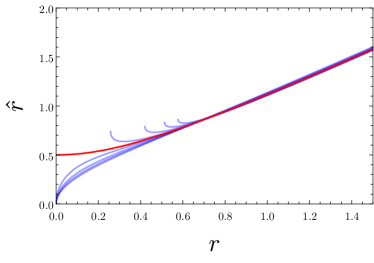
Figure 1: Here we show plots of $\hat{r}$ vs. $r$ for the BTZ black hole (red), and the Gauss–Bonnet corrected BTZ black hole (blue curves). The blue curves lying above the red curve have $\alpha>0$, while those lying below the red curve have $\alpha<0$. In this plot we have fixed $m=1,a=1/2,\ell=1$. The blues curves (from bottom to top) correspond to $\alpha=-1/8$ to $\alpha=+1/8$ in increments of $1/28$. At large-$r$, all cases have $\hat{r}\approx r$.

The metric can be cast into ‘ADM form’, which is commonly used for the rotating BTZ black hole (III.1):

$$ds^{2}=-N^{2}dt^{2}+\hat{r}^{2}\left(N^{\varphi}dt+d\varphi\right)^{2}+\frac{d\hat{r}^{2}}{\hat{f}}\,.$$ (24)

This requires transforming the radial coordinate according to

$$\hat{r}^{2}=-f_{GB}a^{2}+r^{2}\Xi_{\rm eff}^{2}=r^{2}+\frac{2a^{2}m}{\sqrt{X_{\alpha}}+\sqrt{X_{\alpha}-\frac{4\alpha m}{r^{2}}}}\,,$$ (25)

with the lapse and shift given by

$$N^{2}=\frac{r^{2}f_{GB}}{\hat{r}^{2}}\,,\quad N^{\varphi}=\frac{a\Xi_{\rm eff}}{\hat{r}^{2}}\left[f_{GB}-\frac{r^{2}}{\ell_{\rm eff}^{2}}\right]\,,$$ (26)

and analog of the metric function $\hat{f}=1/g_{\hat{r}\hat{r}}$ is

$$\hat{f}_{GB}=\frac{f_{GB}\left[2r\Xi^{2}_{\rm eff}-a^{2}f^{\prime}_{GB}\right]^{2}}{4\hat{r}^{2}}\,.$$ (27)

Inverting (25) to obtain $r(\hat{r})$ is algebraically straightforward, but the resultant expressions are quite cumbersome, and so we plot $\hat{r}$ as a function of $r$ in Fig. 1. For $\alpha>0$, we see that $\hat{r}$ fails to exist beyond the branch singularity (where the spacetime curvature also diverges). For $\alpha<0$, $\hat{r}\to 0$ as $r\to 0$. This is a consequence of the fact mentioned above that $f_{GB}\to 0$ as $r\to 0$. As such, the behaviour of this coordinate is markedly from the ordinary BTZ black hole.

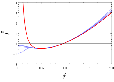
Figure 2: Here we show plots of $\hat{f}$ vs. $\hat{r}$ for the BTZ black hole (red), and the Gauss–Bonnet corrected BTZ black hole (blue curves) with $\alpha<0$. The curves correspond to $\alpha=-1/8$ to $0$ in increments of $1/28$ (top to bottom). We have set the physical parameters $(M,J)=(1,1/2)$ for all cases, with $\ell=1$. At large distances, the metric function behaves as $\hat{f}_{GB}\sim\hat{r}^{2}/\ell_{\rm eff}^{2}$.

We plot the metric function $\hat{f}$ in Fig. 2 instead of presenting the cumbersome expression, with the BTZ case in red. At large distances the metric function behaves as $\hat{f}_{GB}\sim\hat{r}^{2}/\ell_{\rm eff}^{2}$, while near the event horizon the curves are remarkably close to one another. Significant differences appear deep inside the black hole, with the Gauss–Bonnet-BTZ solution failing to exhibit an inner horizon. The behaviour of the lapse is qualitatively the same as $\hat{f}$, with the only notable difference being that $N\to 0$ as $\hat{r}\to 0$ for all negative coupling.

We find that the thermodynamic parameters are now

$$M = \frac{m(2\Xi_{\mbox{\tiny eff}}^{2}-1)}{8}\,,\quad J=\frac{\Xi_{\mbox{\tiny eff}}am}{4}\,,\quad\Omega=\frac{a}{\Xi_{\mbox{\tiny eff}}\ell^{2}_{\mbox{\tiny eff}}}\,,$$

$$T = \frac{f_{GB}^{\prime}}{4\pi\Xi_{\mbox{\tiny eff}}}=\frac{r_{+}}{2\pi\ell^{2}\Xi_{\mbox{\tiny eff}}}\,,\quad S=\frac{\pi\Xi_{\mbox{\tiny eff}}r_{+}}{2}\,,$$

$$P = \frac{1}{8\pi\ell^{2}}\,,\quad V=\pi r_{+}^{2}\Bigl{(}1+\frac{a^{2}}{\ell^{2}\sqrt{X_{\alpha}}}\Bigr{)}\,,$$

$$\psi_{\alpha} = \frac{r_{+}^{2}a^{2}}{16\alpha^{2}\ell^{2}\sqrt{X_{\alpha}}}\Bigl{(}\sqrt{X_{\alpha}}-1-\frac{2\alpha}{\ell^{2}}\Bigr{)}\,,$$ (28)

and obey the respective standard first law and Smarr relation

$$\delta M = T\delta S+\Omega\delta J+V\delta P+\psi_{\alpha}\delta\alpha\,,$$ (29)

$$0 = TS-2PV+\Omega J+2\psi_{\alpha}\alpha\,.$$ (30)

The thermodynamics of this rotating black hole is significantly different from that of its BTZ counterpart: universality of thermodynamics is no longer valid in the presence of rotation. One can easily check that when $\alpha>0$ the isoperimetric ratio Cvetic:2010jb is ${\cal R}=1-\frac{a^{2}}{2\ell^{2}}\frac{\alpha}{\ell^{2}+a^{2}}+O(\alpha^{2})$, indicating that these rotating black holes are super-entropic Hennigar:2014cfa .

IV Rotating black string

It is straightforward to generalize our considerations to $D=4$. We find the following generalization of the black string Lemos:1994xp ; Lemos:1995cm :

$$ds^{2} = -f_{GB}dt^{2}+\frac{dr^{2}}{f_{GB}}+r^{2}d\varphi^{2}+r^{2}dx^{2}\,,\quad\phi=\ln(r/l)\,,$$

$$f_{GB} = \frac{r^{2}}{2\alpha}\Bigl{(}1\pm\sqrt{1-\frac{4\alpha}{r^{2}}f_{E}}\Bigr{)}\,,\quad f_{E}=\frac{r^{2}}{\ell^{2}}-\frac{2M}{r}\,,$$ (31)

and its rotating generalization

$$ds^{2} = -f_{GB}(\Xi_{\mbox{\tiny eff}}dt-ad\varphi)^{2}+\frac{r^{2}}{\ell_{\mbox{\tiny eff}}^{4}}(adt-\Xi_{\mbox{\tiny eff}}\ell_{\mbox{\tiny eff}}^{2}d\varphi)^{2}$$ (32)

$$+\frac{dr^{2}}{f_{GB}}+r^{2}dx^{2}\,,$$

where

$$\Xi_{\mbox{\tiny eff}}=\sqrt{1+\frac{a^{2}}{\ell_{\mbox{\tiny eff}}^{2}}}\,,\quad\ell_{\mbox{\tiny eff}}=\sqrt{\frac{2\alpha}{1-\sqrt{X_{-\alpha}}}}\,,$$ (33)

and the sign difference in $\alpha$ compared to (17) is a consequence of setting $D=4$ in (1).

The thermodynamic quantities (per unit length of the string) are

$$M = \frac{m\Xi_{\mbox{\tiny eff}}(\Xi_{\mbox{\tiny eff}}^{2}+1)}{4}\,,\quad J=\frac{am\Xi_{\mbox{\tiny eff}}^{2}}{4}\,,\quad\Omega=\frac{a}{\Xi_{\mbox{\tiny eff}}\ell^{2}_{\mbox{\tiny eff}}}\,,$$

$$T = \frac{f_{GB}^{\prime}}{4\pi\Xi_{\mbox{\tiny eff}}}=\frac{3}{4}\frac{r_{+}}{\pi\ell^{2}\Xi_{\mbox{\tiny eff}}}\,,\quad S=\frac{\pi\Xi_{\mbox{\tiny eff}}r_{+}^{2}}{2}\,,\quad P=\frac{1}{8\pi\ell^{2}}\,,$$

$$\psi_{\alpha} = \frac{a^{2}r_{+}^{3}}{4\ell^{6}(1+\sqrt{X_{-\alpha}})^{2}\sqrt{X_{-\alpha}}}\sqrt{1\!+\!\frac{2a^{2}}{\ell^{2}(1+\sqrt{X_{-\alpha}})}}\,,$$

$$V = \frac{\pi r_{+}^{3}(a^{2}+4\sqrt{X_{-\alpha}}\ell^{2})}{6\ell^{2}\sqrt{X_{-\alpha}}}\sqrt{1\!+\!\frac{2a^{2}}{\ell^{2}(1+\sqrt{X_{-\alpha}})}}\,,$$ (34)

and obey the standard first law and (4D) Smarr relations:

$$\delta M = T\delta S+\Omega\delta J+V\delta P+\psi_{\alpha}\delta\alpha\,,$$

$$M = 2(TS-PV+\Omega J+\psi_{\alpha}\alpha)\,.$$ (35)

We expect that a similar construction works for black branes if we set $D>4$ in (1) as well, generalizing thus the construction in Awad:2002cz ; Dehghani:2002wn ; Dehghani:2006dh . Contrary to the statements in those paper, however, in order to formulate correct thermodynamics of these objects one needs to employ the effective AdS radius $\ell_{\mbox{\tiny eff}}$ rather than the bare AdS radius $\ell$ in the boost formulae. Once this is done a metric that is non-rotating at infinity is obtained and its thermodynamics (with correct thermodynamic quantities) can be constructed.

V Conclusions

The novel rotating Gauss-Bonnet BTZ black holes obtained in this paper have a number of remarkable properties. As with their BTZ counterparts, they posses an ergoregion and an outer horizon. However they possess no inner horizon – instead they have a cuvature singularity that precludes its formation. If the $\alpha$-dependent terms in (1) arise from quantum gravitational effects, this would be evidence that quantum gravity eliminates unstable inner horizons. Furthermore, rotation breaks the universality of the thermodynamics present in the spherically symmetric case.

We have also also shown that rotating black string solutions exist for $D=4$ Gauss-Bonnet gravity. Their horizon and ergosphere properties are qualitatively similar to the $D=3$ case, and we expect our construction extends to higher-dimensions.

It would be interesting to explore connections between this class of rotating metrics and strong cosmic censorship, which is now known for fail for the rotating BTZ black hole Dias:2019ery ; Balasubramanian:2019qwk . Such a study would provide insight as to the role non-linearity in curvature might play in this regard.

Appendix A Charged Black Holes

The static solution (2)–(4) can be easily generalized to include the effects of the (possibly non-linear) electromagnetic field, by adding the following action:

$$S_{EM}=\int d^{3}x\sqrt{-g}{\cal L}(F)\,,\quad F=F_{ab}F^{ab}\,$$ (36)

to the theory (1). Considering first the Maxwell theory

$${\cal L}_{M}=-F\,,$$ (37)

we find that

$$ds^{2} = -f_{GB}dt^{2}+\frac{dr^{2}}{f_{GB}}+r^{2}d\varphi^{2}\,,$$

$$f^{\pm}_{GB} = -\frac{r^{2}}{2\alpha}\Bigl{(}1\pm\sqrt{1+\frac{4\alpha}{r^{2}}f_{E}}\Bigr{)}\,,\quad\phi=\ln(r/l)\,,\quad$$ (38)

describes for $f^{-}_{GB}$ a charged Gauss–Bonnet BTZ black hole, provided the metric function $f_{E}$ and the vector potential $A$ correspond to those of the charged BTZ black hole in the Einstein gravity Banados:1992wn :

$$f_{E}=\frac{r^{2}}{\ell^{2}}-m-2e^{2}\ln(r/r_{0})\,,\quad A=-e\ln(r/r_{0})dt\,,$$ (39)

with $r_{0}$, $l$, and $m$ arbitrary integration constants.

Similarly, for the Born–Infeld theory born1934foundations ,

$${\cal L}_{BI}=-b^{2}\Bigl{(}\sqrt{1+\frac{2F}{b^{2}}}-1\Bigr{)}\,,$$ (40)

which reduces to the Maxwell Lagrangian (37) in the limit $b\to\infty$, we find that the solution takes the form (38), where now the Einstein metric function $f_{E}$ and vector potential $A$ are those of the Born–Infeld charged BTZ black hole Cataldo:1999wr ; Myung:2008kd :

$$f_{E} = \frac{r^{2}}{\ell^{2}}-m+\frac{1}{2}rb^{2}\Bigl{(}r-\sqrt{r^{2}+r_{1}^{2}}\Bigr{)}$$

$$- \frac{1}{2}r_{0}b^{2}\Bigl{(}r_{0}-\sqrt{r_{0}^{2}+r_{1}^{2}}\Bigr{)}-2e^{2}\ln\left(\frac{r+\sqrt{r^{2}+r_{1}^{2}}}{r_{0}+\sqrt{r_{0}^{2}+r_{1}^{2}}}\right)\,,$$

$$A = -e\ln\left(\frac{r+\sqrt{r^{2}+r_{1}^{2}}}{r_{0}+\sqrt{r_{0}^{2}+r_{1}^{2}}}\right)dt\,,\quad r_{1}=\frac{2e}{b}\,,$$ (41)

where again $r_{0},l,m$ are arbitrary integration constants.

We expect that the form (38) remains valid for charged Gauss–Bonnet BTZ black holes in any theory of non-linear electrodynamics characterized by the action (36). If so, the charged Gauss–Bonnet BTZ black holes share the same horizon radius $r_{+}$ and the same temperature

$$T=\frac{f^{\prime}_{E}(r_{+})}{4\pi}=\frac{f^{\prime}_{GB}(r_{+})}{4\pi}\,$$ (42)

with their Einstein gravity cousins. If their vector fields also coincide, then the thermodynamics is likewise universal.

In particular, for the Born–Infeld theory we have the following thermodynamic quantities:

$$M = \frac{m}{8}\,,\quad T=\frac{f_{E}^{\prime}(r_{+})}{4\pi}=\frac{r_{+}}{2\pi\ell^{2}}\,,\quad S=\frac{1}{2}\pi r_{+}\,,$$

$$Q = e\,,\quad\phi=-\frac{e}{2}\ln\left(\frac{r+\sqrt{r^{2}+r_{1}^{2}}}{r_{0}+\sqrt{r_{0}^{2}+r_{1}^{2}}}\right)\,,$$

$$P = \frac{1}{8\pi\ell^{2}}\,,\quad V=\pi r_{+}^{2}\,,$$ (43)

valid both for the Einstein and Gauss–Bonnet theories. These quantities satisfy the following first law of black hole thermodynamics:

$$\delta M=T\delta S+\phi\delta Q+V\delta P\,,$$ (44)

where we have treated the integration constant $r_{0}$ to be a scale that is independent of the AdS radius $\ell$. To write the corresponding Smarr relation one would need to include the variations the cosmological constant, as well as the variations of $r_{0}$ and of the Born–Infeld parameter $b$ and include the corresponding ‘Born-Infeld polarization’ term into considerations, see Gunasekaran:2012dq . The Maxwell case is recovered upon setting $b\to\infty$.

The obtained solutions in this appendix can be considered as $D=3$ versions of the charged Gauss–Bonnet black holes recently studied in four dimensions Fernandes:2020rpa ; Yang:2020jno . We shall consider extending these solutions to include rotation in a future paper.

References

- (1) D. Lovelock, The Einstein tensor and its generalizations, J. Math. Phys. 12 (1971) 498–501.
- (2) D. Glavan and C. Lin, Einstein-Gauss-Bonnet gravity in 4-dimensional space-time, Phys. Rev. Lett. 124 (2020) 081301, [1905.03601].
- (3) M. Gurses, T. C. Sisman and B. Tekin, Is there a novel Einstein-Gauss-Bonnet theory in four dimensions?, 2004.03390.
- (4) R. A. Hennigar, D. Kubiznak, R. B. Mann and C. Pollack, On Taking the limit of Gauss-Bonnet Gravity: Theory and Solutions, 2004.09472.
- (5) J. Bonifacio, K. Hinterbichler and L. A. Johnson, Amplitudes and 4D Gauss-Bonnet Theory, 2004.10716.
- (6) P. G. Fernandes, P. Carrilho, T. Clifton and D. J. Mulryne, Derivation of Regularized Field Equations for the Einstein-Gauss-Bonnet Theory in Four Dimensions, 2004.08362.
- (7) R. A. Hennigar, D. Kubiznak, R. B. Mann and C. Pollack, Lower-dimensional Gauss–Bonnet Gravity and BTZ Black Holes, 2004.12995.
- (8) R. B. Mann and S. F. Ross, The limit of general relativity, Class. Quant. Grav. 10 (1993) 1405–1408, [gr-qc/9208004].
- (9) H. Lu and Y. Pang, Horndeski Gravity as Limit of Gauss-Bonnet, 2003.11552.
- (10) T. Kobayashi, Effective scalar-tensor description of regularized Lovelock gravity in four dimensions, 2003.12771.
- (11) H. Lu and P. Mao, Asymptotic structure of Einstein-Gauss-Bonnet theory in lower dimensions, 2004.14400.
- (12) M. Banados, C. Teitelboim and J. Zanelli, The Black hole in three-dimensional space-time, Phys. Rev. Lett. 69 (1992) 1849–1851, [hep-th/9204099].
- (13) L. Ma and H. Lu, Vacua and Exact Solutions in Lower- Limits of EGB, 2004.14738.
- (14) S. Ross and R. B. Mann, Gravitationally collapsing dust in (2+1)-dimensions, Phys. Rev. D 47 (1993) 3319–3322, [hep-th/9208036].
- (15) S. Carlip, The (2+1)-Dimensional black hole, Class. Quant. Grav. 12 (1995) 2853–2880, [gr-qc/9506079].
- (16) V. Cardoso and J. P. Lemos, Scalar, electromagnetic and Weyl perturbations of BTZ black holes: Quasinormal modes, Phys. Rev. D 63 (2001) 124015, [gr-qc/0101052].
- (17) R. Konoplya, Influence of the back reaction of the Hawking radiation upon black hole quasinormal modes, Phys. Rev. D 70 (2004) 047503, [hep-th/0406100].
- (18) R. A. Konoplya and A. Zhidenko, BTZ black holes with higher curvature corrections in the 3D Einstein-Lovelock theory, 2003.12171.
- (19) V. Iyer and R. M. Wald, Some properties of Noether charge and a proposal for dynamical black hole entropy, Phys. Rev. D50 (1994) 846–864, [gr-qc/9403028].
- (20) D. Kastor, S. Ray and J. Traschen, Smarr Formula and an Extended First Law for Lovelock Gravity, Class. Quant. Grav. 27 (2010) 235014, [1005.5053].
- (21) M. Cadoni, A. M. Frassino and M. Tuveri, On the universality of thermodynamics and ratio for the charged Lovelock black branes, JHEP 05 (2016) 101, [1602.05593].
- (22) R. A. Hennigar, Criticality for charged black branes, JHEP 09 (2017) 082, [1705.07094].
- (23) J. Lemos, Cylindrical black hole in general relativity, Phys. Lett. B 353 (1995) 46–51, [gr-qc/9404041].
- (24) J. P. Lemos and V. T. Zanchin, Rotating charged black string and three-dimensional black holes, Phys. Rev. D 54 (1996) 3840–3853, [hep-th/9511188].
- (25) G. Gibbons, M. Perry and C. Pope, The First law of thermodynamics for Kerr-anti-de Sitter black holes, Class. Quant. Grav. 22 (2005) 1503–1526, [hep-th/0408217].
- (26) M. Cvetic, G. W. Gibbons, D. Kubiznak and C. N. Pope, Black Hole Enthalpy and an Entropy Inequality for the Thermodynamic Volume, Phys. Rev. D84 (2011) 024037, [1012.2888].
- (27) R. A. Hennigar, D. Kubiznak and R. B. Mann, Entropy Inequality Violations from Ultraspinning Black Holes, Phys. Rev. Lett. 115 (2015) 031101, [1411.4309].
- (28) A. M. Awad, Higher dimensional charged rotating solutions in (A)dS space-times, Class. Quant. Grav. 20 (2003) 2827–2834, [hep-th/0209238].
- (29) M. Dehghani, Charged rotating black branes in anti-de Sitter Einstein-Gauss-Bonnet gravity, Phys. Rev. D 67 (2003) 064017, [hep-th/0211191].
- (30) M. Dehghani and R. B. Mann, Thermodynamics of rotating charged black branes in third order Lovelock gravity and the counterterm method, Phys. Rev. D 73 (2006) 104003, [hep-th/0602243].
- (31) O. J. Dias, H. S. Reall and J. E. Santos, The BTZ black hole violates strong cosmic censorship, JHEP 12 (2019) 097, [1906.08265].
- (32) V. Balasubramanian, A. Kar and G. S rosi, Holographic Probes of Inner Horizons, 1911.12413.
- (33) M. Born and L. Infeld, Foundations of the new field theory, Proceedings of the Royal Society of London. Series A, Containing Papers of a Mathematical and Physical Character 144 (1934) 425–451.
- (34) M. Cataldo and A. Garcia, Three dimensional black hole coupled to the Born-Infeld electrodynamics, Phys. Lett. B 456 (1999) 28–33, [hep-th/9903257].
- (35) Y. S. Myung, Y.-W. Kim and Y.-J. Park, Thermodynamics of Einstein-Born-Infeld black holes in three dimensions, Phys. Rev. D 78 (2008) 044020, [0804.0301].
- (36) A. M. Frassino, R. B. Mann and J. R. Mureika, Lower-Dimensional Black Hole Chemistry, Phys. Rev. D 92 (2015) 124069, [1509.05481].
- (37) M. Appels, L. Cuspinera, R. Gregory, P. Krtouš and D. Kubizňák, Are “Superentropic” black holes superentropic?, JHEP 02 (2020) 195, [1911.12817].
- (38) S. Gunasekaran, R. B. Mann and D. Kubiznak, Extended phase space thermodynamics for charged and rotating black holes and Born-Infeld vacuum polarization, JHEP 11 (2012) 110, [1208.6251].
- (39) P. G. Fernandes, Charged Black Holes in AdS Spaces in Einstein Gauss-Bonnet Gravity, 2003.05491.
- (40) K. Yang, B.-M. Gu, S.-W. Wei and Y.-X. Liu, Born-Infeld Black Holes in novel 4D Einstein-Gauss-Bonnet gravity, 2004.14468.