Tensor Decomposition for Multi-agent Predictive State Representation

Abstract

Predictive state representation (PSR) uses a vector of action-observation sequence to represent the system dynamics and subsequently predicts the probability of future events. It is a concise knowledge representation that is well studied in a single-agent planning problem domain. To the best of our knowledge, there is no existing work on using PSR to solve multi-agent planning problems. Learning a multi-agent PSR model is quite difficult especially with the increasing number of agents, not to mention the complexity of a problem domain. In this paper, we resort to tensor techniques to tackle the challenging task of multi-agent PSR model development problems. By first focusing on a two-agent setting, we construct the system dynamics matrix as a high order tensor for a PSR model, learn the prediction parameters and deduce state vectors directly through two different tensor decomposition methods respectively, and derive the transition parameters via linear regression. Subsequently, we generalize the PSR learning approaches in a multi-agent setting. Experimental results show that our methods can effectively solve multi-agent PSR modelling problems in multiple problem domains.

Keywords Predictive state representations $\cdot$ Tensor optimization $\cdot$ Learning approaches

1 Introduction

Predictive State Representation (PSR) is a dynamic system modelling method and uses a vector of action-observation sequence to represent system states, which is subsequently used to solve a sequence prediction problem [1]. The system dynamics matrix theory provides a matrix-based modelling technique for learning PSR [2]. Currently the PSR discovery and learning algorithms have been well studied except that the algorithmic reliability and efficiency needs to be improved, e.g., the search based techniques [3, 4, 5], the spectral learning approach [6, 7], the compressed sensing approach [8, 9] and the sub-state space method [10]. However, the PSR research is solely conducted in a single-agent decision making setting.

Learning a multi-agent PSR model is rather difficult since available data contains interactive behaviour of multiple agents, e.g. their observations and actions, and the interaction data is often to be considered as a high dimensional space particularly with the increasing number of agents. Moreover, the multi-agent system dynamics matrix is often filled with noise and when the available data is not sufficient in a complicated problem domain, it would be hard to learn a good PSR model in a large multi-agent problem domain. Meanwhile, the computational cost will be dramatically increased since a large number of tests need to be conducted in order to build high dimensional matrices for learning a multi-agent PSR model.

In this paper, we focus on a PSR model with more than one agent and investigate a high dimensional system dynamics matrix, namely tensor, for learning the multi-agent PSR model. The key underlying idea is to take advantage of a highly connected structure of a tensor and the property of tensor decomposition that can extract the latent low-rank components (even though the data is noisy). The difficulty lies in the embedding of tensor into the multi-agent PSR model and the learning of model prediction parameters, state vectors and prediction equation. We present two commonly used tensor decomposition techniques (CP decomposition and its generalized form Tucker decomposition) to solve the PSR discovery and learning problems. Thus, the model prediction parameters and the compressed vector for representing states can be obtained from the decomposition results. Inspired by the transformed PSR model [11], we obtain the model transition parameters via linear regression after constructing auxiliary matrices. We conduct experiments on several problem domains including one extremely large domain, and the results demonstrate the expected performance.

The rest of this paper is organized as follows. In Section 2, we extend a single-agent PSR model, which leads to a multi-agent PSR model, to represent a multi-agent planning problem. Section 3 introduces system dynamics tensor for learning a multi-agent PSR model. Sections 4 and 5 are devoted to the theoretical analysis of learning the multi-agent PSR model of dynamical systems through a tensor decomposition. We present experimental study on several domains in Section 6. In Section 7, we discuss related works on learning PSR. Finally, we conclude our work and give some suggestions on the future work.

2 Technical Background of Multi-agent PSRs

Linear PSRs are a systematic-studied type of PSRs for modelling a dynamic system [1]. The dynamic environment considered here is a discrete-time, controlled dynamic system with $N$-agent ($N\geq 2$), which produces a sequence of actions and observations with one action and one observation per time step. We extend all necessary definitions of a single-agent PSR model to a multi-agent PSR in this section. In order to clearly represent various notations, we use non-bold lowercase letters, boldface lowercase letters, capital letters, calligraphic letters and so on. We summarize a set of main notations in Table 1.

Table 1: Summary of notations

$\textit{a,o,t,h},\phi$	action, observation, test, history, null (joint) history
A,O,T,H	the set of actions, observations, tests and histories
$\text{Q},\textit{D}$	core test set, system dynamics matrix
$m_{t}$	projection vector
$m_{ao},M_{ao}$	(one-step) projection vector and transition matrix
a,o,t,h	joint action, joint observation, joint test, joint history
$\mathcal{A,O,T,H}$	the set of joint actions, joint observations, joint tests and joint histories
$\textbf{Q},\textbf{H},\mathcal{Q}$	core joint test set, core joint history set, core test tensor
$\textbf{D},\mathcal{D}$	system dynamics matrix, system dynamics tensor
$m_{\textbf{t}},m_{{i_{1}}\dots i_{N}}$	projection vector
$m_{\textbf{ao}},M_{\textbf{ao}}$	(one-step) projection vector and transition matrix
$\mathcal{H}_{s}$	joint history set at time step $s$
$\tilde{m}_{*},\tilde{M}_{*}$	projection vector and transition matrix of TPSR
$F$	projection matrix of TPSR
$s$	time step
$\Phi_{d},\Psi_{d}$	training dataset and test dataset
$p(\cdot),p(\cdot|\cdot)$	probabilistic operator and conditional probabilistic operator
$\mathcal{I}(e,\mathcal{S})$	an index that records the index of the element $e$ in set $\mathcal{S}$
$\mathcal{I}(\mathcal{S}^{\prime},\mathcal{S})$	an index set that records the indices of elements of subset $\mathcal{S}^{\prime}$ in set $\mathcal{S}$
$A,A_{i:},A_{:j}$	a matrix, its $i$-th row vector and $j$-th column vector
$A^{T},A^{-1}$	the transpose and (pseudo-)inverse of matrix $A$
$A_{\mathcal{I}}$	a sub-matrix of $A$ consisting of rows indicated by set $\mathcal{I}$
$A^{(i)}$	the $i$-th factor matrix in Tucker decomposition
$\mathcal{A}$	a tensor
$\mathcal{A}_{(k)}$	mode-$k$ matricization of tensor $\mathcal{A}$
$\times_{n}$	the $n$-mode product of a tensor with a matrix
$*,\circ,\otimes$	Hadamard product, outer product, Kronecker product of vectors

2.1 Single-agent PSR

In a controllable dynamical system with a single agent, the agent continuously performs a sequence of actions a chose from the action set $A=\{a^{1},a^{2},\dots,a^{|A|}\}$ according to any policy $\pi$ and senses a sequence of observations o which can be identified in the observation set $O=\{o^{1},o^{2},\dots,o^{|O|}\}$. At time step $s$, the agent has already experienced a sequence of action-observation pairs that are called as history $h$, i.e. $h_{s}=\textit{a}_{1}\textit{o}_{1}\dots\textit{a}_{s}\textit{o}_{s}$ for any possible history at time step $s$. All possible histories at the entire horizon forms a history set $H$. After an agent applies $ao$ at time step $s$, the history $h_{s}$ is updated to history $h_{s+1}=h_{s}ao$. The agent may expect to follow a special sequence of action-observation pairs with the length $l$ which is called as test $t$ beginning immediately at time step $s$, i.e. $t=\textit{a}_{1}\textit{o}_{1}\dots\textit{a}_{l}\textit{o}_{l}$. All possible tests in the future form a test set $T$. The probability of the occurrence of a test $t$ given the history $h_{s}$ is denoted as $p(t|h_{s})$, which can be calculated by prediction equation, thus

$$p(t|h_{s})=f(p(\text{Q}|h_{s}))=p(\text{Q}|h_{s})m_{t}$$

where $f$ is the project function in a linear PSR, $p(\text{Q}|h_{s})$ is the state vector at time step $s$, and $m_{t}$ is the projection vector of test $t$. The new state vector of a linear PSR is calculated by updating equation, thus

$$p(\text{Q}|{h}_{s+1})=\frac{p(\text{Q}|{h}_{s})M_{{ao}}}{p(\text{Q}|{h}_{s}){m}_{{ao}}}$$

where $m_{ao}$ is the projection vector for $t=ao$ and $M_{ao}$ is a matrix consisted of one-step extension projection vectors. In short, a single agent linear PSR model in a controlled partially observable system has the parameters $<{A},{O},\text{Q},\{{m}_{{ao}}\},\{M_{{ao}}\},p(\text{Q}|\phi)>$: the set of actions ${A}$, the set of observations ${O}$, the set of core tests Q, the model parameters ${m}_{{ao}}$ and $M_{{ao}}$ ($\forall\leavevmode\nobreak\ {a}\in{A},{o}\in{O}$), and an initial prediction vector $p(\text{Q}|\phi)$, where $\phi$ is the null history at initial time step $s=0$.

2.2 Multi-agent PSR

For a dynamic $N$-agent system, the joint action $\textbf{a}=a^{(1)}a^{(2)}\cdots a^{(N)}$ represents a sequence of executable actions that agents, e.g. agent (1), $\cdots$, ($N$), can operate simultaneously, and the joint observation $\textbf{o}=o^{(1)}o^{(2)}\cdots o^{(N)}$ represents the observations that the agents may receive in their interactions. Then we have the action set $A^{p}=\{{a}^{1},{a}^{2},\ldots,{a}^{|{A}|-1},{a}^{|{A}|}\}$ to represent all valid actions that agent $p$ can perform, and the observation set $O^{p}=\{{o}^{1},{o}^{2},\ldots,{o}^{|{O}|-1},{o}^{|{O}|}\}$ for all observations that the agent $p$ may receive in the interaction. Hence, we assume that $\mathcal{A}=\{\textbf{a}^{1},\textbf{a}^{2},\ldots,\textbf{a}^{|\mathcal{A}|-1},\textbf{a}^{|\mathcal{A}|}\}$ is a set of all executable joint actions that agents can operate and $\mathcal{O}=\{\textbf{o}^{1},\textbf{o}^{2},\ldots,\textbf{o}^{|\mathcal{O}|-1},\textbf{o}^{|\mathcal{O}|}\}$ is a set of all joint observations that the agents may receive.

A joint test $\textbf{t}=\textbf{a}_{1}\textbf{o}_{1}\textbf{a}_{2}\textbf{o}_{2}\cdots\textbf{a}_{l}\textbf{o}_{l}$ represents the sequence of joint action-observation pairs of all the agents that they may encounter in the future. Accordingly, we have the action sequence $\textbf{t}^{\textbf{a}}=\textbf{a}_{1}\textbf{a}_{2}\cdots\textbf{a}_{l}$ and the observation sequence $\textbf{t}^{\textbf{o}}=\textbf{o}_{1}\textbf{o}_{2}\cdots\textbf{o}_{l}$. The joint test set is a set of all possible joint tests t of the agents, denoted as $\mathcal{T}$. A test is a limited sequence of action-observation pairs in a single agent scenario, e.g., test $t_{i_{1}}^{(i)}=a_{1}^{(i)}o_{1}^{(i)}a_{2}^{(i)}o_{2}^{(i)}\cdots a_{l}^{(i)}o_{l}^{(i)}$ represents the ${i_{1}}$-th sequence of action-observation pairs of the $i$-th agent’s test set $\mathcal{T}^{(i)}$. Then a joint test can be expressed by using the test of all the agents, e.g., $\textbf{t}_{i}=t_{i_{1}}^{(1)}\cdots t_{i_{N}}^{(N)}$, which is the $i$-th joint test in joint test set $\mathcal{T}$. A joint history has the same structure as the joint test, which is used to describe the entire sequence of past action-observation pairs, e.g., joint history $\textbf{h}_{s}=\textbf{a}_{1}\textbf{o}_{1}\textbf{a}_{2}\textbf{o}_{2}\ldots\textbf{a}_{s}\textbf{o}_{s}$ at time step $s$ and the joint history will be updated to $\textbf{h}_{s+1}=\textbf{h}_{s}\textbf{ao}$ after agents taking the joint action a and seeing the joint observation o from the joint history $\textbf{h}_{s}$. The joint history set is a set of all possible joint histories h of the agents, denoted as $\mathcal{H}$. And we denote a joint history set of all possible joint histories $\textbf{h}_{s}$ of the agents with length $s$, denoted as $\mathcal{H}_{s}\subset\mathcal{H}$, i.e., $\mathcal{H}_{s}=\{\textbf{h}|\textbf{h}\in\mathcal{H},|\textbf{h}|=s\}$, which contains all possible joint histories that agents have encountered at time step $s$. Therefore, the joint history set $\mathcal{H}$ can be described as $\mathcal{H}=\{\mathcal{H}_{s=0}=\phi,\mathcal{H}_{s=1},\dots,\mathcal{H}_{s=L}\}$ sampled from training dataset $\Phi_{d}$, where $L$ is max-length of sequences of action-observation in $\Phi_{d}$.

A sequence prediction problem is defined as predicting the probabilities of different joint observation sequences when agents execute the joint action sequence given an arbitrary history. Thus, to make a prediction of a joint test t given the prior joint history $\textbf{h}_{s}\in\mathcal{H}_{s}$ at time step $s$, denoted by $p(\textbf{t}|\textbf{h}_{s})$, is defined as

$$p(\textbf{t}|\textbf{h}_{s})=prob(\textbf{t}^{\textbf{o}}|\textbf{h}_{s}\textbf{t}^{\textbf{a}}).$$ (1)

For any set of joint tests $\textbf{Q}=\{\textbf{q}_{i}|\textbf{q}_{i}\in\mathcal{T},i\in\{1,2,\dots,n\}\}$, its prediction vector (or state vector) is $p(\textbf{Q}|\textbf{h}_{s})=[p(\textbf{q}_{1}|\textbf{h}_{s}),\ldots,p(\textbf{q}_{n}|\textbf{h}_{s})]\in\mathbb{R}^{1\times n}$. If $p(\textbf{Q}|\textbf{h}_{s})$ forms sufficient statistic at any joint history $\textbf{h}_{s}$ in the dynamic system at time step $s$, i.e., all tests can be predicted based on $p(\textbf{Q}|\textbf{h}_{s})$ (in other words, there exists a function $f_{\textbf{t}}$ such that $p(\textbf{t}|\textbf{h}_{s})=f_{\textbf{t}}(p(\textbf{Q}|\textbf{h}_{s}))$ for any test t), then the set Q is called core joint test set. We will denote $p(\textbf{Q}|\textbf{h}_{s}\leftarrow\textbf{h}_{k})$ as $p(\textbf{Q}|\ \textbf{h}_{k})$ for any given joint history $\textbf{h}_{k}\in\mathcal{H}$($k\in[1,|\mathcal{H}|$) at time step $s=|\textbf{h}_{k}|$ for simplicity. For linear PSRs, the function $f_{\textbf{t}}$ is a linear function. Thus, the prediction formula Eq. (1) can be rewritten as

$$p(\textbf{t}|\textbf{h}_{s})=p(\textbf{Q}|\textbf{h}_{s}){m}_{\textbf{t}},$$ (2)

where ${m}_{\textbf{t}}\in\mathbb{R}^{n\times 1}$ is called projection vector. For $\textbf{t}_{i}=t_{i_{1}}^{(1)}\cdots t_{i_{N}}^{(N)}$, Eq. (2) becomes

$$p(t_{i_{1}}^{(1)}\cdots t_{i_{N}}^{(N)}|\textbf{h}_{s})=p(\textbf{Q}|\textbf{h}_{s}){m}_{t_{i_{1}},\dots,t_{i_{N}}},$$

we will denote ${m}_{t_{i_{1}},\dots,t_{i_{N}}}$ as ${m}_{{i_{1}}\dots i_{N}}$ for simplicity. For example, in a 2-agent system, the projection vector for a joint test $\textbf{t}=t_{i}^{(1)}t_{j}^{(2)}$ can be denoted by ${m}_{ij}$. The projection vector for a one-step joint test $\textbf{t}=\textbf{ao}$ in a multi-agent system is denoted by $m_{\textbf{ao}}$.

When a system receives the agents’ joint action a, it immediately transforms into a next state, which means the PSR model should update its state at the same time. The update calculates the new state $p(\textbf{Q}|\textbf{h}_{s+1})$ from the previous state $p(\textbf{Q}|\textbf{h}_{s})$ after agents take the joint action a and receive the observation o from the history $\textbf{h}_{s}$. The initial state is $p(\textbf{Q}|\phi)$ when $\textbf{h}_{s}$ takes the null joint history $\phi$ at time step $s=0$. For any core joint test $\textbf{q}_{i}\in\textbf{Q}$ and $\textbf{h}_{s+1}=\textbf{h}_{s}\textbf{ao}$, $\forall\,\textbf{a}\in\mathcal{A},\textbf{o}\in\mathcal{O}$, we compute the update as follows:

$$p(\textbf{q}_{i}|\textbf{h}_{s+1})=\frac{p(\textbf{ao}\textbf{q}_{i}|\textbf{h}_{s})}{p(\textbf{ao}|\textbf{h}_{s})}=\frac{p(\textbf{Q}|\textbf{h}_{s}){m}_{\textbf{ao}\textbf{q}_{i}}}{p(\textbf{Q}|\textbf{h}_{s}){m}_{\textbf{ao}}},$$ (3)

where ${m}_{\textbf{ao}}$ and ${m}_{\textbf{aoq}_{i}}$ are ${m}_{\textbf{t}}$ for each one-step joint test (ao) and each one-step extension ($\textbf{ao}\textbf{q}_{i}$) respectively. The first equality of Eq. (3) is obtained by Bayes rule, and the second one is computed by Eq. (2). By defining the matrix $M_{\textbf{ao}}\in\mathbb{R}^{n\times n}$, in which the $i$-th column vector is ${m}_{\textbf{ao}\textbf{q}_{i}}$, we have

$$M_{\textbf{ao}}=[{m}_{\textbf{ao}\textbf{q}_{1}}\leavevmode\nobreak\ \leavevmode\nobreak\ {m}_{\textbf{ao}\textbf{q}_{2}}\leavevmode\nobreak\ \leavevmode\nobreak\ \cdots\leavevmode\nobreak\ \leavevmode\nobreak\ {m}_{\textbf{ao}\textbf{q}_{n}}],\leavevmode\nobreak\ \leavevmode\nobreak\ \forall\,\textbf{a}\in\mathcal{A},\textbf{o}\in\mathcal{O}.$$

Subsequently, Eq. (3) can be rewritten as

$$p(\textbf{Q}|\textbf{h}_{s+1})=\frac{p(\textbf{Q}|\textbf{h}_{s})M_{\textbf{ao}}}{p(\textbf{Q}|\textbf{h}_{s}){m}_{\textbf{ao}}}.$$ (4)

The vectors {${m}_{\textbf{ao}}$} and matrices $\{M_{\textbf{ao}}\}$ ($\forall\textbf{a}\in\mathcal{A},\textbf{o}\in\mathcal{O})$ are called the model parameters of the linear PSR model. If an initial prediction vector $p(\textbf{Q}|\phi)$ for a given null joint history $\phi$, the prediction vector $p(\textbf{Q}|\textbf{h}_{s})$ can be calculated step by step for any time $s$. In addition, for any test $\textbf{t}=\textbf{a}_{1}\textbf{o}_{1}\textbf{a}_{2}\textbf{o}_{2}\cdots\textbf{a}_{l}\textbf{o}_{l}$, its corresponding projection vector $m_{\textbf{t}}$ can be computed by the chain rule in terms of conditional probability, Eqs. (1) and (4), i.e.,

$$m_{\textbf{t}}=M_{\textbf{a}_{1}\textbf{o}_{1}}M_{\textbf{a}_{2}\textbf{o}_{2}}\cdots M_{\textbf{a}_{l-1}\textbf{o}_{l-1}}m_{\textbf{a}_{l}\textbf{o}_{l}}.$$

Notice that when the model parameters and the initial prediction vector of the linear PSR model are known, i.e., the modelling of the entire PSR model is completed, we can make the sequential prediction $p(\textbf{t}|\textbf{h})$. If the core joint tests Q is found, the parameters can be computed as follows.

$$\begin{array}[]{l}{m}_{\textbf{ao}}=p(\textbf{Q}|\textbf{H})^{-1}p(\textbf{ao}|\textbf{H}),\\ {m}_{\textbf{aoq}_{i}}=p(\textbf{Q}|\textbf{H})^{-1}p(\textbf{aoq}_{i}|\textbf{H}),\end{array}$$

where H is called core joint history set. The values of $p(\textbf{Q}|\textbf{H}),$ $p(\textbf{ao}|\textbf{H})$ and $p(\textbf{aoq}_{i}|\textbf{H})$ can be estimated through the training data in the following.

$$p(\textbf{Q}|\textbf{H})=\begin{bmatrix}p(\textbf{q}_{1}|\textbf{h}_{1})&p(\textbf{q}_{2}|\textbf{h}_{1})&\cdots&p(\textbf{q}_{n}|\textbf{h}_{1})\\ p(\textbf{q}_{1}|\textbf{h}_{2})&p(\textbf{q}_{2}|\textbf{h}_{2})&\cdots&p(\textbf{q}_{n}|\textbf{h}_{2})\\ \vdots&\vdots&\ddots&\vdots\\ p(\textbf{q}_{1}|\textbf{h}_{|\textbf{H}|})&p(\textbf{q}_{2}|\textbf{h}_{|\textbf{H}|})&\cdots&p(\textbf{q}_{n}|\textbf{h}_{|\textbf{H}|})\end{bmatrix},$$

$$p(\textbf{ao}|\textbf{H})=\begin{bmatrix}p(\textbf{ao}|\textbf{h}_{1})\\ p(\textbf{ao}|\textbf{h}_{2})\\ \vdots\\ p(\textbf{ao}|\textbf{h}_{|\textbf{H}|})\end{bmatrix},\leavevmode\nobreak\ \text{and}\quad p(\textbf{aoq}_{i}|\textbf{H})=\begin{bmatrix}p(\textbf{aoq}_{i}|\textbf{h}_{1})\\ p(\textbf{aoq}_{i}|\textbf{h}_{2})\\ \vdots\\ p(\textbf{aoq}_{i}|\textbf{h}_{|\textbf{H}|})\end{bmatrix}.$$

In a summary, a linear PSR model in a controlled partially observable system has the parameters $<\mathcal{A},\mathcal{O},\textbf{Q},\{{m}_{\textbf{ao}}\},\{M_{\textbf{ao}}\},p(\textbf{Q}|\phi)>$: the set of joint actions $\mathcal{A}$, the set of joint observations $\mathcal{O}$, the set of core joint tests Q, the model parameters ${m}_{\textbf{ao}}$ and $M_{\textbf{ao}}$ ($\forall\leavevmode\nobreak\ \textbf{a}\in\mathcal{A},\textbf{o}\in\mathcal{O}$), and an initial prediction vector $p(\textbf{Q}|\phi)$, where $\phi$ is the null joint history. The process of finding Q is called the discovery problem, while the computation of the projection vectors by using Q to represent all the other tests is called the learning problem.

In a variant of PSRs, transformed predictive representation (TPSR) [11] tries to maintain a small number of linear combinations of the probabilities of a larger number of tests instead of maintaining probability distributions over the outcomes of a small set of tests. Therefore, we are aiming to learn a multi-agent PSR model based on TPSR in this paper. Traditionally, the parameters $<\mathcal{A},\mathcal{O},x_{s},\{\tilde{m}_{\textbf{ao}}\},\{\tilde{M}_{\textbf{ao}}\},x_{0}>$ describes a TPSR model, where $x_{s}$ is the compressed state vector, $x_{0}$ is an initial compressed state vector and the other parameters are the same as a usual linear PSR model. In fact, $x_{s}$ is a compressed version of system prediction vector $p(\textbf{Q}|\textbf{h}_{s})$, and hence $x_{0}$ is a reduced version of an initial prediction vector $p(\textbf{Q}|\textbf{h}_{s=0}=\phi)$. Therefore, $x_{s}\in\mathbb{R}^{1\times R}$ can be calculated by multiplying $p(\textbf{Q}|\textbf{h}_{s})$ by a projection matrix ${F}$, namely:

$$x_{s}=p(\textbf{Q}|\textbf{h}_{s}){F},$$ (5)

where the matrix ${F}\in\mathbb{\mathbb{R}}^{|\textbf{Q}|\times R}$, $|\textbf{Q}|$ is the size of core joint test set Q. Therefore, for a given joint history $\textbf{h}_{k}\in\mathcal{H}$($k\in[1,|\mathcal{H}|]$) at time step $s=|\textbf{h}_{k}|$, we have $x_{s}=p(\textbf{Q}|\textbf{h}_{k}){F}$ and can denote $x_{s}$ as $x_{k}$ for simplicity. Hence, for a given joint history $\textbf{h}_{k}\in\mathcal{H}$($k\in[1,|\mathcal{H}|]$) at time step $s=|\textbf{h}_{k}|$, the prediction formula Eq. (2) and the state update Eq. (4) can be rewritten as

$$p(\textbf{t}|\textbf{h}_{k})=x_{k}\tilde{m}_{\textbf{t}},$$ (6)

and

$$x_{k+1}=\frac{x_{k}\tilde{M}_{\textbf{ao}}}{x_{k}\tilde{m}_{\textbf{ao}}},$$ (7)

where $\tilde{m}_{\textbf{ao}}\in\mathbb{R}^{R\times 1}$ is called a projection vector or model prediction parameter, which can be calculated in Eqs. (2), (5) and (6), i.e., $\tilde{m}_{\textbf{ao}}={F}^{-1}m_{\textbf{ao}}$ , and $\tilde{M}_{\textbf{ao}}\in\mathbb{R}^{R\times R}$ is called a transition matrix or model update parameter, which can be calculated in Eqs. (4), (5), (7) and $\tilde{m}_{\textbf{ao}}={F}^{-1}m_{\textbf{ao}}$, i.e., $\tilde{M}_{\textbf{ao}}={F}^{-1}M_{\textbf{ao}}{F}$. However, it is difficult to solve the transformation matrix ${F}$ directly in order to learn the model parameters. Generally, the two parameters learned for TPSR will not be identical to those learned in a traditional PSR model. It can no longer interpret the elements of $x_{k}$ as probabilities as they may be negative or even larger than 1. Since the two parameters fully summary the system updating rule and sequential prediction, we will learn them in another way without the help of the projection matrix ${F}$ in this paper.

3 System Dynamics Tensor for Multi-agent PSRs

In this section, we construct the system dynamics matrix as a high order tensor for learning a multi-agent PSR model, and give the formulas to calculate the system marginal dynamic matrix and the PSR model under each agent’s perspective. The PSR model of each agent can be used to predict its future sequences given the experienced history of the system.

We propose a system dynamics tensor for learning a multi-agent PSR model based on a tensor approach. For a system with $N$ agents, we use $\mathcal{D}\in\mathbb{\mathbb{R}}^{n_{1}\times n_{2}\times n_{3}\times\cdots\times n_{N+1}}$ to denote a system dynamics tensor, whose element is $\mathcal{D}_{i_{1}i_{2}\cdots i_{N}k}=p(t_{i_{1}}^{(1)}\dots t_{i_{N}}^{(N)}|\textbf{h}_{k})$, which can be estimated by the reset algorithm [3], where $t_{i_{1}}^{(1)}$, $t_{i_{2}}^{(2)}$, $\ldots$, $t_{i_{N}}^{(N)}$ are the tests for each agent and $\textbf{h}_{k}\in\mathcal{H}$($k\in[1,|\mathcal{H}|)$) is the given joint history at time step $s=|\textbf{h}_{k}|$. Then, the discovery problem is transferred into finding a minimal linearly independent set (i.e., core joint test set Q), so that the whole fibers listed in the set Q form a basis of the space spanned by the mode-$(N+1)$ fibers of tensor $\mathcal{D}$, and these fibers together form a sub-tensor, namely core test tensor $\mathcal{Q}$.

Without loss of generality, let us discuss a 2-agent scenario, the system dynamic tensor $\mathcal{D}\in\mathbb{\mathbb{R}}^{n_{1}\times n_{2}\times n_{3}}$ is a 3rd order tensor now, where $n_{3}=|\mathcal{H}|$ and $n_{i}=|\mathcal{T}^{(i)}|(i=1,2)$, as intuitively shown in Fig. 1. Its element, e.g., $p(t_{1}^{(1)}t_{2}^{(2)}|{\textbf{a}^{1}\textbf{o}^{1}})$, is corresponding to the test $t_{1}^{(1)}={a^{1}o^{2}}$ in test set $\mathcal{T}^{(1)}$ of agent 1, the test $t_{2}^{(2)}={a^{2}o^{2}}$ in test set $\mathcal{T}^{(2)}$ of agent 2, and the joint history ${\textbf{a}^{1}\textbf{o}^{1}}$ in joint history set $\mathcal{H}$. The corresponding system marginal dynamics matrices (i.e., $D^{(1)}\in\mathbb{\mathbb{R}}^{|\mathcal{T}^{(1)}|\times|\mathcal{H}^{(1)}|}$ and $D^{(2)}\in\mathbb{\mathbb{R}}^{|\mathcal{T}^{(2)}|\times|\mathcal{H}^{(2)}|}$) can be calculated by the elements of system dynamics tensor $\mathcal{D}$ according to the probability theory. Let us take the computation of $D^{(1)}$ as an example. For any $\textbf{t}^{(1)}\in\mathcal{T}^{(1)}$, $\textbf{h}^{(1)}\in\mathcal{H}^{(1)}$, the element $D^{(1)}_{\textbf{t}^{(1)},\textbf{h}^{(1)}}$ is computed as follows:

$$D^{(1)}_{\textbf{t}^{(1)},\textbf{h}^{(1)}} = {p(\textbf{t}^{(1)}|\textbf{h}^{(1)})}$$

$$= \sum_{\textbf{h}^{(2)},|\textbf{h}^{(2)}|=|\textbf{h}^{(1)}|}\leavevmode\nobreak\ \leavevmode\nobreak\ {\sum_{\textbf{t}^{(2)},|\textbf{t}^{(2)}|=|\textbf{t}^{(1)}|}{p(\textbf{t}^{(1)}\textbf{t}^{(2)}|\textbf{h}^{(1)}\textbf{h}^{(2)})}}$$

$$= \sum_{\textbf{h}^{(2)},|\textbf{h}^{(2)}|=|\textbf{h}^{(1)}|}\leavevmode\nobreak\ \leavevmode\nobreak\ {\sum_{\textbf{t}^{(2)},|\textbf{t}^{(2)}|=|\textbf{t}^{(1)}|}{\mathcal{D}_{\textbf{t}^{(1)}\textbf{t}^{(2)},\textbf{h}^{(1)}\textbf{h}^{(2)}}}},$$

where the second equation is obtained by summing up all the histories and tests of all the other agents (i.e., agent 2 in this case) with length $|\textbf{h}^{(2)}|=|\textbf{h}^{(1)}|$ and $|\textbf{t}^{(2)}|=|\textbf{t}^{(1)}|$, marked as two red directions on the upper left hand side of Fig. 1. For simplicity, we write the two system marginal dynamics matrices as follows.

$$\begin{aligned} D^{(1)}=\sum_{\textbf{h}^{(2)}\in\mathcal{H}^{(2)}}{\sum_{\textbf{t}^{(2)}\in\mathcal{T}^{(2)}}\mathcal{D}},\leavevmode\nobreak\ \text{and}\quad D^{(2)}=\sum_{\textbf{h}^{(1)}\in\mathcal{H}^{(1)}}{\sum_{\textbf{t}^{(1)}\in\mathcal{T}^{(1)}}\mathcal{D}}\end{aligned}.$$

The two dimensions of each matrix reflect test and history, respectively.

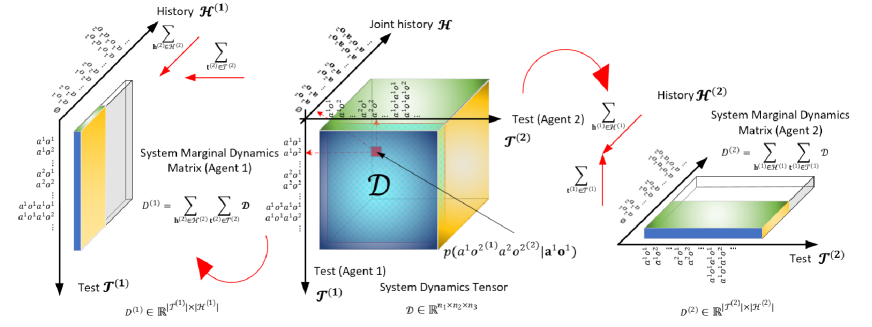
Figure 1: Diagram of system marginal dynamics matrices obtained by system dynamics tensor of 2-agent system

On the other hand, the system dynamics matrix [1] can be employed for learning a multi-agent PSR model as an alternative way since we will apply the traditional matrix-based single-agent PSR learning algorithms to the multi-agent PSRs in Section 6.1.2. The matrix consists of joint histories and tests, and their elements can be estimated by the reset algorithm [3]. The difference between system dynamics matrix and system dynamics tensor is that we put the joint tests of all the agents in only one dimension when constructing a system dynamics matrix.

For a two-agent system, the system dynamics matrix $\textbf{D}\in\mathbb{\mathbb{R}}^{|\mathcal{T}|\times|\mathcal{H}|}$ can be depicted as a two-dimensional matrix in Fig. 2. For example, the element $p({\textbf{a}^{2}\textbf{o}^{1}}|{\textbf{a}^{1}\textbf{o}^{1}})$ of matrix D is corresponding to the joint test $\textbf{a}^{2}\textbf{o}^{1}$ in the joint test set $\mathcal{T}$, and the joint history ${\textbf{a}^{1}\textbf{o}^{1}}$ in the joint history set $\mathcal{H}$. The corresponding system marginal dynamics matrices (i.e., $D^{(1)}\in\mathbb{\mathbb{R}}^{|\mathcal{T}^{(1)}|\times|\mathcal{H}^{(1)}|}$ and $D^{(2)}\in\mathbb{\mathbb{R}}^{|\mathcal{T}^{(2)}|\times|\mathcal{H}^{(2)}|}$) can be obtained by the elements of matrix D. Let us take the calculation of $D^{(1)}$ as an example. For any $\textbf{t}^{(1)}\in\mathcal{T}^{(1)}$, $\textbf{h}^{(1)}\in\mathcal{H}^{(1)}$, the element $D^{(1)}_{\textbf{t}^{(1)},\textbf{h}^{(1)}}$ is calculated below.

$$D^{(1)}_{\textbf{t}^{(1)},\textbf{h}^{(1)}} = p(\textbf{t}^{(1)}|\textbf{h}^{(1)})$$

$$= \sum_{\textbf{h}^{(2)},|\textbf{h}^{(2)}|=|\textbf{h}^{(1)}|}\leavevmode\nobreak\ \leavevmode\nobreak\ {\sum_{\textbf{t}^{(2)},|\textbf{t}^{(2)}|=|\textbf{t}^{(1)}|}{p(\textbf{t}^{(1)}\textbf{t}^{(2)}|\textbf{h}^{(1)}\textbf{h}^{(2)})}}$$

$$= \sum_{\textbf{h}^{(2)},|\textbf{h}^{(2)}|=|\textbf{h}^{(1)}|}\leavevmode\nobreak\ \leavevmode\nobreak\ {\sum_{\textbf{t}^{(2)},|\textbf{t}^{(2)}|=|\textbf{t}^{(1)}|}{\textbf{D}_{\textbf{t}^{(1)}\textbf{t}^{(2)},\textbf{h}^{(1)}\textbf{h}^{(2)}}}},$$

where the second equation is obtained by summing up all the histories and testes of all the other agents (i.e., agent 2 in this case) with length $|\textbf{h}^{(2)}|=|\textbf{h}^{(1)}|$ and $|\textbf{t}^{(2)}|=|\textbf{t}^{(1)}|$, as shown in the left hand side of Fig. 2. Hence, the two dimensions of $D^{(1)}$ reflect history and test of agent 1, respectively. For simplicity, we write the two system marginal dynamics matrices as follows.

$$D^{(1)}=\sum_{\textbf{h}^{(2)}\in\mathcal{H}^{(2)}}{\sum_{\textbf{t}^{(2)}\in\mathcal{T}^{(2)}}\textbf{D}},\leavevmode\nobreak\ \text{and}\quad D^{(2)}=\sum_{\textbf{h}^{(1)}\in\mathcal{H}^{(1)}}{\sum_{\textbf{t}^{(1)}\in\mathcal{T}^{(1)}}\textbf{D}}.$$

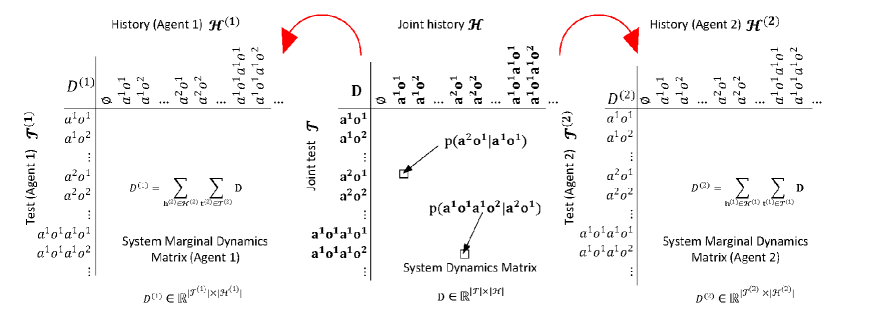
Figure 2: Diagram of system marginal dynamics matrices obtained by the system dynamics matrix of 2-agent system

Correspondingly, the system PSR model in the perspective of two agents has the following parameters.

$$\left\{\begin{aligned} <\mathcal{A}^{(1)},\mathcal{O}^{(1)},\textbf{Q}^{(1)},\{\sum_{\textbf{ao}^{(2)}}{m}_{\textbf{ao}}\},\{\sum_{\textbf{ao}^{(2)}}M_{\textbf{ao}}\},\sum_{\textbf{Q}^{(2)}}p(\textbf{Q}|\phi)>\\ <\mathcal{A}^{(2)},\mathcal{O}^{(2)},\textbf{Q}^{(2)},\{\sum_{\textbf{ao}^{(1)}}{m}_{\textbf{ao}}\},\{\sum_{\textbf{ao}^{(1)}}M_{\textbf{ao}}\},\sum_{\textbf{Q}^{(1)}}p(\textbf{Q}|\phi)>\end{aligned}\right..$$

Similarly, for a general multi-agent system, the system marginal dynamics matrices can be obtained by the system dynamics tensor $\mathcal{D}$ and the system dynamics matrix D respectively, and the PSR model of each agent can also be directly obtained from the learned multi-agent PSR model, namely:

$$\left\{\begin{aligned} D^{(1)}&=\sum_{\textbf{h}^{(\neq 1)}\in\mathcal{H}^{(\neq 1)}}{\sum_{\textbf{t}^{(\neq 1)}\in\mathcal{T}^{(\neq 1)}}\mathcal{D}}\\ &\vdots\\ D^{(N)}&=\sum_{\textbf{h}^{(\neq N)}\in\mathcal{H}^{(\neq N)}}{\sum_{\textbf{t}^{(\neq N)}\in\mathcal{T}^{(\neq N)}}\mathcal{D}}\end{aligned}\right.\leavevmode\nobreak\ \text{and}\quad\left\{\begin{aligned} D^{(1)}&=\sum_{\textbf{h}^{(\neq 1)}\in\mathcal{H}^{(\neq 1)}}{\sum_{\textbf{t}^{(\neq 1)}\in\mathcal{T}^{(\neq 1)}}\textbf{D}}\\ &\vdots\\ D^{(N)}&=\sum_{\textbf{h}^{(\neq N)}\in\mathcal{H}^{(\neq N)}}{\sum_{\textbf{t}^{(\neq N)}\in\mathcal{T}^{(\neq N)}}\textbf{D}}\end{aligned}\right.,$$

and

$$\left\{\begin{aligned} <\mathcal{A}^{(1)},\mathcal{O}^{(1)},\textbf{Q}^{(1)},\{\sum_{\textbf{ao}^{(\neq 1)}}{m}_{\textbf{ao}}\},\{\sum_{\textbf{ao}^{(\neq 1)}}M_{\textbf{ao}}\},\sum_{\textbf{Q}^{(\neq 1)}}p(\textbf{Q}|\phi)>\\ \vdots\hskip 200.0003pt\\ <\mathcal{A}^{(N)},\mathcal{O}^{(N)},\textbf{Q}^{(N)},\{\sum_{\textbf{ao}^{(\neq N)}}{m}_{\textbf{ao}}\},\{\sum_{\textbf{ao}^{(\neq N)}}M_{\textbf{ao}}\},\sum_{\textbf{Q}^{(\neq N)}}p(\textbf{Q}|\phi)>\\ \end{aligned}\right..$$

Accordingly we can use these matrices and the PSR model for individual agent planning.

4 Learning 2-agent PSR via Tensor Decomposition

In this section, we propose a new framework for learning 2-agent PSR via tensor decomposition. We elaborate how to obtain the prediction parameters $\tilde{m}_{ij}$ and the state vector $x_{k}$ of the PSR model through CP decomposition (CP) and Tucker decomposition (TD) respectively, and then use a linear regression to learn the transition parameters $\tilde{M}_{\textbf{ao}}$ of the model from the training data.

4.1 Learning Prediction Parameters and State Vectors

After obtaining interactive data $\Phi_{d}$ between two agents, we construct the system dynamics tensor $\mathcal{D}\in\mathbb{\mathbb{R}}^{n_{1}\times n_{2}\times n_{3}}$, whose element is $\mathcal{D}_{ijk}=p(t_{i}^{(1)}t_{j}^{(2)}|\textbf{h}_{k})$, where $t_{i}^{(1)}$ is the $i$-th test sequence of the $1$st agent’s test set $\mathcal{T}^{(1)}$, $t_{j}^{(2)}$ is the $j$-th test sequence of the $2$nd agent’s test set $\mathcal{T}^{(2)}$ and $\textbf{h}_{k}\in\mathcal{H}$($k\in[1,|\mathcal{H}|)$) is the given joint history at time step $s=|\textbf{h}_{k}|$. We use two main tensor decomposition approaches on tensor $\mathcal{D}$ for learning the prediction parameters and the state vector respectively.

4.1.1 CP Decomposition Learning Method

The CP decomposition decomposes a tensor into a sum of rank-one tensors that can be concisely written in Eq. (8).

$$\mathcal{D}\approx[\textbf{$\lambda$};A,B,C]\equiv\sum^{R}_{r=1}\lambda_{r}a_{r}\circ b_{r}\circ c_{r},$$ (8)

where $R$ is a positive integer, “$\circ$” denotes outer product of vectors, and $\lambda_{r}\in\mathbb{R}$, $a_{r}\in\mathbb{R}^{n_{1}}$, $b_{r}\in\mathbb{R}^{n_{2}}$ and $c_{r}\in\mathbb{R}^{n_{3}}$ for $r=1,2,\ldots,R$. The factor matrices $A$, $B$ and $C$ consist of the vectors, i.e., $A=[a_{1}\ a_{2}\ \cdots\ a_{R}]\in\mathbb{\mathbb{R}}^{n_{1}\times R}$, $B=[b_{1}\ b_{2}\ \cdots\ b_{R}]\in\mathbb{\mathbb{R}}^{n_{2}\times R}$ and $C=[c_{1}\ c_{2}\ \cdots\ c_{R}]\in\mathbb{\mathbb{R}}^{n_{3}\times R}$. For any $i\in\{1,\ldots,n_{1}\}$, $j\in\{1,\ldots,n_{2}\}$ and $k\in\{1,\ldots,n_{3}\}$, we observe that each element of the tensor $\mathcal{D}$ can be written in Eq. (9).

$$\mathcal{D}_{ijk}=\sum^{R}_{r=1}\lambda_{r}A_{ir}B_{jr}C_{kr},$$ (9)

where $A_{ir}$ is the $(i,r)$-th element of matrix $A$, and likewise for $B_{jr}$ and $C_{kr}$, for $r=1,2,\ldots,R$.

Let $x_{k}=[x_{k}(1)\cdots x_{k}(R)]\in\mathbb{\mathbb{R}}^{1\times R}$, $k\in\{1,\ldots,n_{3}\}$ be the $k$-th row vector $C_{k:}$. Since the joint histories of dynamic system stored in the 3rd dimension of the tensor $\mathcal{D}$ are compressed in the matrix $C$, its row vector $x_{k}$ is a summary of joint history $\textbf{h}_{k}\in\mathcal{H}$($k\in[1,|\mathcal{H}|$) and can be considered as a compressed version of the system state vector $p(\textbf{Q}|\textbf{h}_{k})$ at time step $s=|\textbf{h}_{k}|$. On the other hand, for any $r\in\{1,2,\ldots,R\}$, we define the scalar $\tilde{m}_{ij}(r)=\lambda_{r}A_{ir}B_{jr}$, and then construct the column vector $\tilde{m}_{ij}={[\tilde{m}_{ij}(1)\ \tilde{m}_{ij}(2)\ \cdots\ \tilde{m}_{ij}(R)]}^{T}\in\mathbb{\mathbb{R}}^{R}$. Thus, we have

$$\tilde{m}_{ij}=(\lambda\ast A_{i:}\ast B_{j:})^{T},$$ (10)

where $\lambda=[\lambda_{1}\cdots\lambda_{R}]\in\mathbb{\mathbb{R}}^{1\times R}$, “$\ast$” denotes the Hadamard product (vector element-wise product), $A_{i:}$ denotes the $i$-th row vector of $A$ and likewise for $B_{j:}$. Then, from (6), we rewrite Eq. (9) as

$$\mathcal{D}_{ijk}=\sum^{R}_{r=1}\tilde{m}_{ij}(r)x_{k}(r)=x_{k}(\lambda\ast A_{i:}\ast B_{j:})^{T}=x_{k}\tilde{m}_{ij}.$$

Hence, the prediction parameters $\tilde{m}_{ij}$ and the compressed state vector $x_{k}$ are obtained from the tensor decomposition results. Remark that we do not compute $x_{k}$ directly from Eq. (5), and $p(\textbf{Q}|\textbf{h}_{k})$ and $F$ are unknown currently.

The computation process of learning the prediction parameters $\tilde{m}_{ij}$ and the compressed state vector $x_{k}$ by CP decomposition is shown in Fig. 3. After applying the CP decomposition to the system dynamics tensor, we have 3 factor matrices and a diagonal tensor in Step 1. For each element $\mathcal{D}_{ijk}$ in tensor $\mathcal{D}$, it can be realized by the CP decomposition results shown in Step 2. Hence, we can deduce the prediction parameters from $\mathcal{D}_{ijk}$ in Step 3. Moreover, the system state vector is also obtained for a further use.

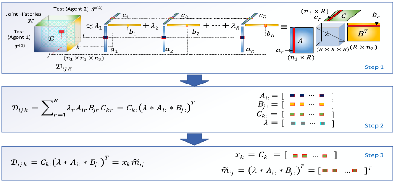
Figure 3: The process of learning the prediction parameters $\tilde{m}_{ij}$ and the compressed state vector $x_{k}$ by CP decomposition

4.1.2 Tucker Decomposition Learning Method

The Tucker decomposition decomposes a tensor into a core tensor multiplied (or transformed) by a matrix along each mode, i.e.,

$$\mathcal{D}\approx[\mathcal{G};A,B,C]\equiv\mathcal{G}\times_{1}A\times_{2}B\times_{3}C\hskip 35.00005pt$$

$$=\sum^{P}_{p=1}\sum^{Q}_{q=1}\sum^{R}_{r=1}g_{pqr}a_{p}\circ b_{q}\circ c_{r},$$ (11)

where “$\times_{k}$” denotes $k$-mode product of tensor $\mathcal{G}$ by a matrix with appropriate dimensions and $P,Q,R$ are all positive integers. Usually $P<n_{1}$, $Q<n_{2}$ and $R<n_{3}$, the core tensor $\mathcal{G}$ can be thought of as a compressed version of $\mathcal{D}$. The factor matrices $A,B$ and $C$ can be computed in Eq. 12. $A=[a_{1}\ a_{2}\ \cdots\ a_{P}]\in\mathbb{\mathbb{R}}^{n_{1}\times P}$, $B=[b_{1}\ b_{2}\ \cdots\ b_{Q}]\in\mathbb{\mathbb{R}}^{n_{2}\times Q}$ and $C=[c_{1}\ c_{2}\ \cdots\ c_{R}]\in\mathbb{\mathbb{R}}^{n_{3}\times R}$. Similarly, each element of the tensor $\mathcal{D}$ can be written as

$$\mathcal{D}_{ijk}=\sum^{P}_{p=1}\sum^{Q}_{q=1}\sum^{R}_{r=1}g_{pqr}A_{ip}B_{jq}C_{kr}.$$ (12)

Let $x_{k}=[x_{k}(1)\cdots x_{k}(R)]\in\mathbb{\mathbb{R}}^{1\times R}$, $k\in\{1,\ldots,n_{3}\}$ be the $k$-th row vector $C_{k:}$. As discussed in Section 4.1.1, the row vector of $C$ is the compressed state vector $x_{k}$ of the TPSR model. For any $r\in\{1,2,\ldots,R\}$, we define the scalar $\tilde{m}_{ij}(r)=\sum^{P}_{p=1}\sum^{Q}_{q=1}g_{pqr}A_{ip}B_{jq}$, and construct the column vector $\tilde{m}_{ij}={[\tilde{m}_{ij}(1)\ \tilde{m}_{ij}(2)\ \cdots\ \tilde{m}_{ij}(R)]}^{T}\in\mathbb{\mathbb{R}}^{R}$. Thus, we get

$$\tilde{m}_{ij}=\mathcal{G}_{(3)}(B_{j:}\otimes A_{i:})^{T},$$ (13)

where “$\otimes$” denotes Kronecker product, and $\mathcal{G}_{(3)}$ is the mode-3 unfolding of the core tensor $\mathcal{G}$. Hence, from Eq. (6), Eq. (12) becomes

$$\mathcal{D}_{ijk}=\sum^{R}_{r=1}\tilde{m}_{ij}(r)x_{k}(r)=x_{k}\tilde{m}_{ij}.$$

The computation process of learning the prediction parameters $\tilde{m}_{ij}$ and the compressed state vector $x_{k}$ by Tucker decomposition is shown in Fig. 4. Similarly, we obtain 3 factor matrices and a core tensor after applying the Tucker decomposition in Step 1. Then in Step 2, each element $\mathcal{D}_{ijk}$ can be reorganized by the Tucker decomposition results. Hence, we can deduce the prediction parameters in Step 3 and the system state vector as well.

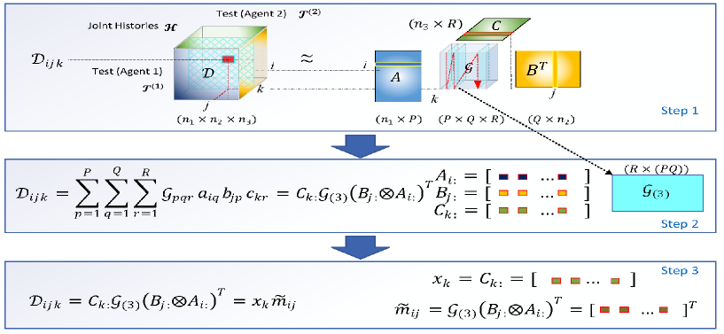
Figure 4: The process of learning the prediction parameters $\tilde{m}_{ij}$ and the compressed state vector $x_{k}$ by Tucker decomposition

We may add some proper constraints to Equations (8) and (11) to ensure solution uniqueness or algorithm convergence in the tensor decompositions. We assume that the norm of all columns of $A,B$ and $C$ are 1 for Eq. (8), and $A,B$ and $C$ are column-wise orthonormal for problem (11). If we further add non-negative constraints on $A,B$ and $C$, the problems become non-negative CP decomposition (NCP) and non-negative Tucker decomposition (NTD), respectively. There are many methods devoted for solving these NP-hard problems (in general), and the corresponding algorithms may converge to a stationary point and enjoy convergence guarantee under certain conditions, see e.g., [12], [13] and [14].

4.2 Learning Transition Parameters

In Section 4.1, we have derived the prediction parameters $\{\tilde{m}_{ij}\}$ for the TPSR model through two tensor decomposition methods respectively, see Steps 1-2 of Fig. 5. From the analysis in Section 2, we can find the subset of one-step projection vectors $\{\tilde{m}_{\textbf{ao}}\}$ from the prediction parameter set $\{\tilde{m}_{ij}\}$ for each $\textbf{a}\textbf{o}\in\mathcal{A}\times\mathcal{O}$, which is important in learning the model transition parameters $M_{\textbf{ao}}$. In addition, we know that it is very difficult and not necessary to get the transformation matrix ${F}$. Therefore, we try to learn the model transition parameters $M_{\textbf{ao}}$ through a linear regression from the training data, see Steps 3-4 of Fig. 5.

For any $\textbf{a}\in\mathcal{A},\textbf{o}\in\mathcal{O}$, we find all the joint histories $\textbf{h}\in\mathcal{H}$ ending with action-observation ao and construct a subset of joint history set $\mathcal{H}$, i.e., $\mathcal{H}^{\prime}_{\textbf{ao}}=\{\textbf{h}|\textbf{h}=\textbf{h}^{\prime}\textbf{ao},\textbf{h}\in\mathcal{H},\textbf{h}^{\prime}\in\mathcal{H}\}$. Moreover, for every joint history $\textbf{h}^{\prime}\in\mathcal{H}^{\prime}_{\textbf{ao}}$, we cut off the action-observation ao, obtain the new joint history $\textbf{h}=\textbf{h}^{\prime}\setminus\textbf{ao}$ which absolutely belongs to the joint history set $\mathcal{H}$, and then construct a subset of joint history set $\mathcal{H}$, i.e., $\mathcal{H}^{\prime}=\{\textbf{h}|\textbf{h}=\textbf{h}^{\prime}\setminus\textbf{ao},\textbf{h}\in\mathcal{H},\textbf{h}^{\prime}\in\mathcal{H}^{\prime}_{\textbf{ao}}\}$. We see that the size of the joint history set $\mathcal{H}^{\prime}$ is equal to that of the joint history set $\mathcal{H}^{\prime}_{\textbf{ao}}$, i.e., $|\mathcal{H}^{\prime}|=|\mathcal{H}^{\prime}_{\textbf{ao}}|$.

Let $\mathcal{I}(\mathcal{H}^{\prime},\mathcal{H})$ be an index set that records the indices of each element of the subset $\mathcal{H}^{\prime}$ in the set $\mathcal{H}$. Particularly, $\mathcal{I}(\textbf{h}_{k}\in\mathcal{H}^{\prime},\mathcal{H})$ is an index that records the index of joint history $\textbf{h}_{k}\in\mathcal{H}^{\prime}$ in the set $\mathcal{H}$. Given $x_{k}\leavevmode\nobreak\ (k\in\mathcal{I}(\mathcal{H}^{\prime},\mathcal{H}))$, we multiply both sides of Eq. (7) by ${x_{k}\tilde{m}_{\textbf{ao}}}$, and obtain a series of equations with a size equal to $|\mathcal{H}^{\prime}|$. Thus, we have

$$\left\{\begin{aligned} x_{\mathcal{I}(\textbf{h}_{1}^{\prime}\in\mathcal{H}^{\prime}_{\textbf{ao}},\mathcal{H})}x_{\mathcal{I}(\textbf{h}_{1}\in\mathcal{H}^{\prime},\mathcal{H})}\tilde{m}_{\textbf{ao}}&=x_{\mathcal{I}(\textbf{h}_{1}\in\mathcal{H}^{\prime},\mathcal{H})}\tilde{M}_{\textbf{ao}}\\ x_{\mathcal{I}(\textbf{h}_{2}^{\prime}\in\mathcal{H}^{\prime}_{\textbf{ao}},\mathcal{H})}x_{\mathcal{I}(\textbf{h}_{2}\in\mathcal{H}^{\prime},\mathcal{H})}\tilde{m}_{\textbf{ao}}&=x_{\mathcal{I}(\textbf{h}_{2}\in\mathcal{H}^{\prime},\mathcal{H})}\tilde{M}_{\textbf{ao}}\\ \vdots\hskip 20.00003pt&=\hskip 10.00002pt\vdots\\ x_{\mathcal{I}(\textbf{h}_{|\mathcal{H}^{\prime}_{\textbf{ao}}|}^{\prime}\in\mathcal{H}^{\prime}_{\textbf{ao}},\mathcal{H})}x_{\mathcal{I}(\textbf{h}_{|\mathcal{H}^{\prime}|}\in\mathcal{H}^{\prime},\mathcal{H})}\tilde{m}_{\textbf{ao}}&=x_{\mathcal{I}(\textbf{h}_{|\mathcal{H}^{\prime}|}\in\mathcal{H}^{\prime},\mathcal{H})}\tilde{M}_{\textbf{ao}}\end{aligned}\right.,$$

where $\textbf{h}_{k}^{\prime}=\textbf{h}_{k}\textbf{ao}$, $k=1,2,\ldots,|\mathcal{H}^{\prime}|$ and the subscripts $\mathcal{I}(\textbf{h}_{k}^{\prime}\in\mathcal{H}^{\prime}_{\textbf{ao}},\mathcal{H})$ and $\mathcal{I}(\textbf{h}_{k}\in\mathcal{H}^{\prime},\mathcal{H})$ indicate the row indices of the factor matrix $C$. Then, we extract the row $x_{\mathcal{I}(\textbf{h}_{k}\in\mathcal{H}^{\prime},\mathcal{H})}$ from $C$ according to the index $\mathcal{I}(\textbf{h}_{k}\in\mathcal{H}^{\prime},\mathcal{H})$, and construct the system state matrix $X\in\mathbb{\mathbb{R}}^{|\mathcal{H}^{\prime}|\times R}$, i.e., $X\leftarrow C_{\mathcal{I}(\mathcal{H}^{\prime},\mathcal{H})}$. Similarly, we extract the row $x_{\mathcal{I}(\textbf{h}_{k}^{\prime}\in\mathcal{H}^{\prime}_{\textbf{ao}},\mathcal{H})}$ from $C$ and construct the one-step extension system state matrix $X_{\textbf{ao}}\in\mathbb{\mathbb{R}}^{|\mathcal{H}^{\prime}_{\textbf{ao}}|\times R}$, i.e., $X_{\textbf{ao}}\leftarrow C_{\mathcal{I}(\mathcal{H}_{\textbf{ao}}^{\prime},\mathcal{H})}$. For simplicity, we denote $C_{\mathcal{I}(\mathcal{H}^{\prime},\mathcal{H})}$ and $C_{\mathcal{I}(\mathcal{H}^{\prime}_{\textbf{ao}},\mathcal{H})}$ as $C_{\mathcal{H}^{\prime}}$ and $C_{\mathcal{H}^{\prime}_{\textbf{ao}}}$, respectively. Hence, we have

$$X=\begin{bmatrix}x_{\mathcal{I}(\textbf{h}_{1}\in\mathcal{H}^{\prime},\mathcal{H})}\\ x_{\mathcal{I}(\textbf{h}_{2}\in\mathcal{H}^{\prime},\mathcal{H})}\\ \vdots\\ x_{\mathcal{I}(\textbf{h}_{|\mathcal{H}^{\prime}|}\in\mathcal{H}^{\prime},\mathcal{H})}\end{bmatrix},\leavevmode\nobreak\ \text{and}\quad X_{\textbf{ao}}=\begin{bmatrix}x_{\mathcal{I}(\textbf{h}_{1}^{\prime}\in\mathcal{H}^{\prime}_{\textbf{ao}},\mathcal{H})}\\ x_{\mathcal{I}(\textbf{h}_{2}^{\prime}\in\mathcal{H}^{\prime}_{\textbf{ao}},\mathcal{H})}\\ \vdots\\ x_{\mathcal{I}(\textbf{h}_{|\mathcal{H}^{\prime}_{\textbf{ao}}|}^{\prime}\in\mathcal{H}^{\prime}_{\textbf{ao}},\mathcal{H})}\end{bmatrix}.$$

Let $d_{\textbf{ao}}=X\tilde{m}_{\textbf{ao}}$, and $D_{\textbf{ao}}$ be the matrix with $d_{\textbf{ao}}$ on its diagonal. Thus, Eq. (4.2) can be written as

$$D_{\textbf{ao}}X_{\textbf{ao}}=X\tilde{M}_{\textbf{ao}}.$$ (14)

The value $\tilde{M}_{\textbf{ao}}$ will be exactly true if we have a perfect estimation of $X$, $X_{\textbf{ao}}$ and $\tilde{m}_{\textbf{ao}}$ from infinite training data. With finite training data, it is generally not possible to have precise $\tilde{M}_{\textbf{ao}}$ in Eq. (14). Hence we formulate the following optimization problem below

$$\min\limits_{\tilde{M}}\dfrac{1}{2}\|D_{\textbf{ao}}X_{\textbf{ao}}-X\tilde{M}\|_{F}^{2},$$

where $\|\cdot\|_{F}$ is the Frobenius norm of a matrix. Taking derivative on $\tilde{M}$, we have the optimal solution

$$\tilde{M}^{*}_{\textbf{ao}}={(X^{T}X)}^{-1}(X^{T}D_{\textbf{ao}}X_{\textbf{ao}}).$$ (15)

Fig. 5 shows the detailed calculations of $\tilde{m}_{\textbf{ao}}$, $\tilde{M}_{\textbf{ao}}$, and $X$, $X_{\textbf{ao}}$ and $D_{\textbf{ao}}$ as well. As shown in the figure, we offer two frameworks for decomposing the tensor, and obtain a state matrix $C$, which means that the state vector of state matrix $C$ is updated while the system updates along the red dashed link after receiving the joint action-observation ao. After applying tensor decomposition (either CP or Tucker) to the system dynamics tensor $\mathcal{D}$ (Step 1), we immediately obtain the prediction parameters $\tilde{m}_{\textbf{ao}}$ in Step 2. In Step 3, starting from the joint histories of the longest action-observation sequences (L), the process goes: \small{1}⃝ finds out all the rows of $C$ corresponding to the action-observation sequence ending with ao, which can be indexed by the elements of joint history set $\mathcal{H}^{\prime}_{\textbf{ao}}$; \small{2}⃝ finds out the corresponding rows of $C$ after deleting ao, which can be indexed by the elements of joint history set $\mathcal{H}^{\prime}$; \small{3}⃝ puts the row vectors from \small{1}⃝ into the matrix $X_{\textbf{ao}}$; \small{4}⃝ puts the row vectors from \small{2}⃝ into the matrix $X$; \small{5}⃝-\small{7}⃝ repeat from \small{1}⃝ to \small{4}⃝ until the empty sequences appear. Finally, we calculate $\tilde{M}_{\textbf{ao}}$ in Eq. (15) in Step 4.

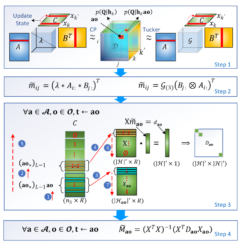
Figure 5: Tensor decomposition for learning 2-agent PSR

5 Multi-agent PSR via Tensor Decomposition

We extend the learning 2-agent PSR model to the case of multiple agents. Given a dynamic system has $N$ agents, we have tensor $\mathcal{D}\in\mathbb{\mathbb{R}}^{n_{1}\times n_{2}\times n_{3}\times\cdots\times n_{N+1}}$, whose element is $\mathcal{D}_{i_{1}i_{2}\dots i_{N}k}=p(t_{i_{1}}^{(1)}\cdots t_{i_{N}}^{(N)}|\textbf{h}_{k})$ . Its CP decomposition:

$$\mathcal{D} \approx[\textbf{$\lambda$};A^{(1)},A^{(2)},\dots,A^{({N+1})}]$$

$$\equiv\sum^{R}_{r=1}\lambda_{r}a_{r}^{(1)}\circ a_{r}^{(2)}\circ\cdots\circ a_{r}^{{({N+1})}},$$

and its Tucker decomposition:

$$\mathcal{D} \approx[\mathcal{G};A^{(1)},A^{(2)},\dots,A^{({N+1})}]$$

$$\equiv\mathcal{G}\times_{1}A^{(1)}\times_{2}A^{(2)}\times_{3}\cdots\times_{N+1}A^{({N+1})}\hskip 42.00003pt\hskip 25.00003pt$$

$$=\sum^{R_{1}}_{r_{1}=1}\sum^{R_{2}}_{r_{2}=1}\cdots\sum^{R_{N+1}}_{r_{N+1}=1}g_{r_{1}r_{2}\dots r_{N+1}}a_{r_{1}}^{(1)}\circ a_{r_{2}}^{(2)}\circ\cdots\circ a_{r_{N+1}}^{({N+1})}.$$

Therefore, analogous to Section 4, we have the prediction parameters of the PSR model

$$\tilde{m}_{i_{1}\dots i_{N}}=(\lambda\ast A_{i_{1}:}^{(1)}\ast A_{i_{2}:}^{(2)}\ast\cdots\ast A_{i_{N}:}^{({N})})^{T},$$ (16)

$$\tilde{m}_{i_{1}\dots i_{N}}=\mathcal{G}_{(N+1)}(A_{i_{N}:}^{({N})}\otimes A_{i_{N-1}:}^{({N-1})}\otimes\dots\otimes A_{i_{1}:}^{(1)})^{T},$$ (17)

via CP and Tucker decomposition methods, respectively. The state vector is given by

$$x_{k}=A_{k:}^{({N+1})},$$ (18)

and the transition matrix is

$$\tilde{M}_{\textbf{ao}}={(X^{T}X)}^{-1}(X^{T}D_{\textbf{ao}}X_{\textbf{ao}}).$$ (19)

after constructing $X$ and $X_{\textbf{ao}}$, computing $d_{\textbf{ao}}$ and constructing $D_{\textbf{ao}}$.

Algorithm 5 summarizes the learning procedures. First, we construct the system dynamics tensor $\mathcal{D}$ from agents’ interaction data set $\Phi_{d}$ (line 1). We then apply either CP or Tucker decomposition to the system dynamics tensor $\mathcal{D}$, and obtain the prediction parameters $\tilde{m}_{i_{1}\dots i_{N}}$ through Eq. (16) or Eq. (17) (lines 2-8). Subsequently, we compute the state vector $x_{k}$ by Eq. (18) (lines 9-11). For any $\textbf{a}\in\mathcal{A},\textbf{o}\in\mathcal{O}$, we construct the matrices $X$ and $X_{\textbf{ao}}$ in Step 3 of Fig. 5 (lines 13-16), compute vector $d_{\textbf{ao}}$ and construct matrix $D_{\textbf{ao}}$ with $d_{\textbf{ao}}$ on its diagonal (lines 17-20), and then compute the transition matrix $\tilde{M}_{\textbf{ao}}$ by Eq. (19) (line 21). Finally, we get all the parameters that are needed in order to learn a multi-agent PSR model.

  Algorithm 1: Tensor-based algorithm for learning multi-agent PSR   Data: number of agents $N$, agents’ interaction data $\Phi_{d}$, decomposition $Methods$ (CP or Tucker), dimension of state compression $R$ (or $(R_{1},R_{2},\dots,R_{N+1})$).

Result: system state vector $x_{k}$, model parameters $\tilde{M}_{i_{1}\dots i_{N}}$ and $\tilde{m}_{i_{1}\dots i_{N}}$.

1 Construct system dynamics tensor $\mathcal{D}$ from data $\Phi_{d}$;

2 if $Method=CP$ then

3       $[A^{(1)},A^{(2)},\dots,A^{({N+1})}]\leftarrow CP(\mathcal{D},R)$;

4       $\tilde{m}_{i_{1}\dots i_{N}}\leftarrow(\lambda*A_{i_{1}:}^{(1)}*A_{i_{2}:}^{(2)}*\cdots*A_{i_{N}:}^{({N})})^{T}$;

5      

6else

7       $[\mathcal{G},A^{(1)},A^{(2)},\dots,A^{({N+1})}]=Tucker(\mathcal{D},(R_{1},R_{2},\dots,R_{N+1}))$;

8       $\tilde{m}_{i_{1}\dots i_{N}}\leftarrow\mathcal{G}_{(N+1)}(A_{i_{N}:}^{({N})}\otimes A_{i_{N-1}:}^{({N-1})}\otimes\cdots\otimes A_{i_{1}:}^{(1)})^{T}$;

9      

10 end if

11foreach $k\in\{1,\dots,n_{N+1}\}$ do

12       $x_{k}\leftarrow A_{k:}^{({N+1})}$;

13      

14 end foreach

15foreach $\textbf{a}\in\mathcal{A},\textbf{o}\in\mathcal{O}$ do

16       $\mathcal{H}^{\prime}_{\textbf{ao}}\leftarrow\{\textbf{h}|\textbf{h}=\textbf{h}^{\prime}\textbf{ao},\textbf{h}\in\mathcal{H},\textbf{h}^{\prime}\in\mathcal{H}\}$;

17       $\mathcal{H}^{\prime}\leftarrow\{\textbf{h}|\textbf{h}=\textbf{h}^{\prime}\setminus\textbf{ao},\textbf{h}\in\mathcal{H},\textbf{h}^{\prime}\in\mathcal{H}^{\prime}_{\textbf{ao}}\}$;

18       $X\leftarrow C_{\mathcal{H}^{\prime}}$ ;

19       $X_{\textbf{ao}}\leftarrow C_{\mathcal{H}^{\prime}_{\textbf{ao}}}$;

20       $\textbf{t}\leftarrow\textbf{ao}$;

21       $\tilde{m}_{\textbf{ao}}\leftarrow\tilde{m}_{\textbf{t}}$;

22       $d_{\textbf{ao}}\leftarrow X\tilde{m}_{\textbf{ao}}$;

23       $D_{\textbf{ao}}\leftarrow diag(d_{\textbf{ao}}^{1},\ldots,d_{\textbf{ao}}^{|\mathcal{H}^{\prime}|})$;

24       $\tilde{M}_{\textbf{ao}}\leftarrow{(X^{T}X)}^{-1}(X^{T}D_{\textbf{ao}}X_{\textbf{ao}})$;

25      

26 end foreach

 

6 Experimental Study

We implement the prediction models in the platform of MATLAB, and all the computations are conducted on a Windows PC with a 16-core Intel E5-2640 2.60 GHz CPU and 64 GB memory. In order to evaluate the learnt PSR models, a series of action-observation sequences (whose length ranges from 1 to 15) are needed to test and evaluate the predictive performance of the models in various problem domains. Therefore, we test our approach on four extended versions of standard benchmarks taken from the literatures, i.e., Tag [15], Gridworld$*$ [8], ColoredGridworld$*$ [9] and Poc-Man$*$ [16]. Moreover, we simply add one more agent in domains Tag and Gridworld$*$ to construct 3-agent systems for testing purpose. All of them are large domains and were originally defined in a partially observable Markov decision process (POMDP) [17].

For every problem domain $d$, agents are given a random exploration strategy to continuously execute actions in the environment to obtain observations. This is to construct the training sample set $\Phi_{d}$ and the test sample set $\Psi_{d}$. In the training sample set $\Phi_{d}$, there were 2000 action-observation sequences each of which is with a maximum length of 10 (because some sequences would terminate early, e.g., reaching the target). There are 3000 action-observation sequences each of which has a maximum length of 15 in the test sample set $\Psi_{d}$.

We conduct 20 experiments (rounds) to evaluate the average performance of each model in every domain. In every test, the single-round test training set used in model training is randomly selected from the training sequence set $\Phi_{d}$, which has 500 action-observation sequences ( Poc-Man$*$ uses 400 training sequences, considering that it has a relatively large state space), while the single-round test set used in the test has about 1000 action-observation sequences, which is also randomly selected from $\Psi_{d}$.

6.1 Experimental Settings

6.1.1 Problem Domains

\small{1}⃝ Tag

The domain Tag depicted in Fig. 6 is a test-bed proposed for multi-agent research [15, 18], in which a chasing Robot tracks and tags its Opponent in an uncertain environment. There is a set of five executable actions $A=\{\textit{North, East, South, West, Tag}\}$ for Robot, while $A=\{\textit{North, East, South, West, Noop}\}$ for Opponent. Each agent receives a -1 bonus for each move. If they are in the same grid, Robot can fully observe Opponent and should perform $Tag$ action to win a +10 reward; otherwise, a negative bonus -10 is returned. The Opponent moves away from Robot with a chance of 0.8, otherwise stays still. If Opponent is tagged, the game is over and Opponent will obtain a -10 bonus. After agents have performed any action, each agent can sensor the surrounding in four directions and receive a noisy observation $o_{i}$ to check whether there are any walls blocking its movement. Therefore, the space of the agents’ observation is $O=\{o_{1},o_{2},\dots,o_{16}\}$. The state space for Robot is $S=\{s_{1},s_{2},\dots,s_{29}\}$ and Opponent is $S=\{s_{1},s_{2},\dots,s_{29},s_{tagged}\}$, which is a set of all possible locations plus with a special tagged state $s_{tagged}$.

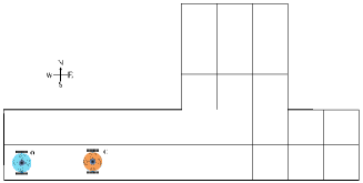
Figure 6: Tag with a medium number of states and observations.

\small{2}⃝ Gridworld$*$ and ColoredGridworld$*$

The domains GridWorld$*$ and ColoredGridWorld$*$ are a direct extension of the domain GridWorld [9, 8]. All these domains have a 5 $\times$ 12 grid maze (see Fig. 7), in which agents must navigate from a fixed start state towards a goal grid. The main difference between them lies in the different responses of the environment to the interactions performed by agents or the different observation that the agents receive. In GridWorld$*$, an agent can sensor the surrounding in four directions and receive a noisy observation to check whether there are any walls blocking its movement, which results in $2^{4}$ possible observations. While in ColoredGridWorld$*$, the agent can see colored walls with three possible colors. Hence there are 3 possible observations per wall, which results in $2^{8}$ possible observations in total. In addition, the complexity of colored walls increases the size of observation space exponentially, which results in a huge set of possible tests and histories. The set of all executable actions of each agent is $A=\{\textit{North, East, South, West}\}$. An agent fails to execute an action with the probability 0.2. If this happens, the agent randomly moves in a direction orthogonal to the specified direction. A reward of 1 is returned at the target state (resetting the environment) and a negative bonus -1 is costed for each move of the agent. The state space of the agent is a set of all possible locations plus with a goal state $s_{52}$, i.e., $S=\{s_{1},s_{2},\dots,s_{52}\}$.

(a) Gridworld

(b) ColoredGridworld

Figure 7: Gridworld$*$ and ColoredGridworld$*$ with a medium number of states and observations.The grid with red circle is the goal grid.

\small{3}⃝ Poc-Man$*$

The Poc-Man$*$ domain is commonly used for examining the performance of PSR models, which is a variant of the popular video game Pac-Man [16]. In Poc-Man$*$, the two agents (marked by yellow points in Fig. 8) navigate in the maze, gather randomly placed food pellets and keep away from four ghosts (marked by red points in Fig. 8) just like in the game scenario Pac-Man. However, in this domain, the agents can only use noisy and partial observations about local environment states to accomplish their mission, which is not identical to the video game version. The set of all executable actions of each agent is $A=\{\textit{North, East, South, West}\}$. An agent fails to execute an action with probability 0.2. If this happens, each agent randomly moves in a direction orthogonal to the specified direction. After the agents have performed any action, they can sensor the surrounding in four directions and receive a noisy observation to check whether there are any walls blocking its movement.

Meanwhile, a reward of 1 is returned when each agent finds food pellets and a negative bonus -1 is costed for each move of each agent. Learning a perfect predictive representation of this domain is a challenging task because it has a large size of state space($\lvert\mathcal{S}\rvert\approx 10^{56}$) and observation space($\lvert\mathcal{O}\rvert\approx 2^{18}$).

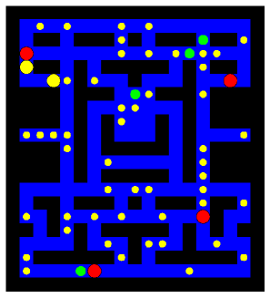
Figure 8: Pocman$*$ with a large number of states and observations.

In summary, these domains have different sizes of observation space and state space, which represents different uncertainties and randomness of dynamic systems. In Table 2, we list the size of the action space, observation space and system state space of each domain for comparative analysis. Meanwhile, we also show the relationship between the agents in each domain.

Table 2: Structure of each domain

Domain	$|\mathcal{A}|=|A\times A|$	$|\mathcal{O}|=|O\times O|$	$|\mathcal{S}|=|S\times S|$	Relationship
Tag	$5\times 5$	$2^{4}\times 2^{4}$	870	Competitive
Gridworld$*$	$4\times 4$	$2^{4}\times 2^{4}$	2704	Competitive
ColoredGridworld$*$	$4\times 4$	$2^{8}\times 2^{8}$	2704	Competitive
Poc-Man$*$	$4\times 4$	$\approx 2^{9}\times 2^{9}$	$\approx 10^{56}$	Cooperative

6.1.2 Comparative Methods

We aim to learn a complete PSR model in different multi-agent systems as elaborated above. Note that many algorithms focus on learning a local model of the underlying system with the aim of making only predictions in specific situations. Thus, these algorithms are not included in the comparison. For all domains, we compare our new learning PSRs techniques (CP, NCP, TD and NTD) to traditional methods, i.e., TPSR and compressed PSR (CPSR) approaches [9, 8]. For a fair comparison, we set the compressed dimension of our algorithms ($R$ in CP (NCP) and $(P,Q,R)$ in TD (NTD)) to be the same as that of TPSR and CPSR algorithms.

6.1.3 Performance Measurements

The main purpose of a dynamic system is to predict the probabilities of different observations when executing an action given an arbitrary history. We evaluate the learnt models in terms of prediction accuracy, which computes the gap between the true predictions and the predictions given by the learnt model over all test sequences. For each domain, there are no related POMDP files, which contains the true value of each step prediction or could obtain through calculating. Hence, we cannot obtain the true predictions and use Monte-Carlo roll-out predictions [8] instead.

The error function used in our experiments is called absolute error (AE) that computes the average of absolute error of one-step prediction error per time step given an arbitrary history $\textbf{h}_{k}$ at time step $s=|\textbf{h}_{k}|$, as shown in Eq. (20).

$$AE=\frac{1}{N_{T}}\sum_{t=1}^{N_{T}}\lvert\hat{p}(\textbf{o}_{k+1}^{t}|\textbf{h}_{k}^{t}\textbf{a}_{k+1}^{t})-p(\textbf{o}_{k+1}^{t}|\textbf{h}_{k}^{t}\textbf{a}_{k+1}^{t})\rvert.$$ (20)

where $N_{T}$ is the total number of test sequences ($N_{T}=1000\times 20$), which is equal to the size of single-round test set times the total number of rounds, and the test of length $k$ starting from 0 to $L-1$ ($L=15$) are used, respectively. In Eq. (20), $p(\cdot)$ is the probability obtained from the Monte-Carlo roll-out prediction and $\hat{p}(\cdot)$ is the estimated probability computed by the learnt model.

6.2 Results

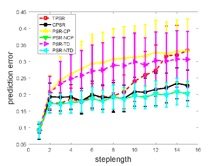
(a) Gridworld$*$

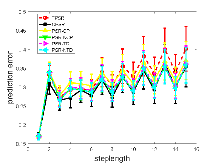
(b) ColoredGridworld$*$

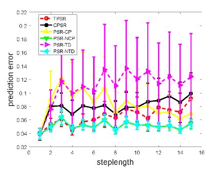
(c) Poc-man$*$

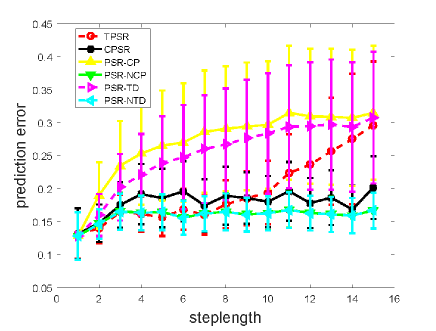
(d) Tag

Figure 9: Comparison analysis of tensor methods, TPSR and CPSR for 2-agent domains Gridworld$*$, GridworldColor$*$, Poc-Man$*$ and Tag

We conduct the experiments to calculate the model accuracy by comparing the one-step prediction accuracy of the evaluated methods in six problem domains (2-agent domains including Tag, Gridworld$*$, ColoredGridworld$*$, and Poc-Man$*$, and 3-agent domains including Tag and Gridworld$*$), and the average runtime for each domain is also obtained.

In Fig. 9, the $x$-axis is the step length of action-observation and the $y$-axis is the mean prediction error of 20,000 trials ($N_{T}=1000\times 20$) calculated by Eq. (20). As it can be seen from Fig. 9, for almost all cases in 2-agent system, our algorithms (PSR-CP and PSR-TD) perform as well as all the other algorithms, but are not very well when the step-length is bigger than two except ColoredGridworld$*$. While PSR-NCP and PSR-NTD perform best and produce more competitive predictions than other algorithms in all horizons for all domains. As shown in Fig. 9(c), both PSR-NCP and PSR-NTD algorithm are able to learn more accurate models compared to the TPSR and CPSR algorithms in the Poc-Man$*$ domain, although the domain is more suitable for the CPSR approach. The reason why PSR-NCP and PSR-NTD are technically superior to their competitors is due to the fact that they get a non-negative solution, while CP and TD optimizations do not have a nonnegativity constraint.

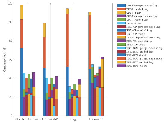
Figure 10: Runtime in building and testing the models for four different 2-agent domains

The running time of each algorithm is given in Fig. 10, including the time of three parts:

\small{1}⃝ Data preprocessing includes establishing and normalizing the dynamics matrix (tensor) of the system and the auxiliary matrices of an algorithm. When an algorithm needs more auxiliary matrices, the computational time will inevitably increase. Especially with the extension of the action-observation sequence or the increasing complexity of a problem domain, the dynamics matrix will eventually become very large. Compared to our methods, TPSR and CPSR methods cost much more time.

\small{2}⃝ Modelling includes finding the core joint test set of PSR and learning model parameters. TPSR and CPSR need to perform singular value decomposition (SVD) operations on the dynamics matrix, and our algorithms need to solve tensor decomposition problems. Our methods perform as well as TPSR and CPSR methods in this part. With the benefit of tensor decomposition, we can truly improve the efficiency of the algorithm.

\small{3}⃝ Making prediction. In Poc-Man$*$, our methods spend more time than the others because our methods obtain a larger set of projection vectors, which costs much time to the state update of the model when the prediction is carried out.

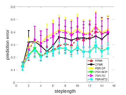
(a) Gridworld$*$ ($N=3$)

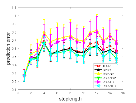
(b) Tag ($N=3$)

Figure 11: Comparison analysis of tensor methods, TPSR and CPSR for 3-agent domains Gridworld$*$ and Tag

In Fig. 11, we add one more agent for domain Gridworld$*$ and a Robot agent for domain Tag. For all horizons of these two domains, PSR-NCP and PSR-NTD perform better than all the other algorithms and produce more competitive predictions. This also show the scalability of our approaches in this article.

In summary, the good performance of our approach is partially due to the fact that the tensor decomposition can dig out the embedded connections of high dimensional data and it is not largely effected by noise in the dynamic system.

7 Related Works

Predictive state representation (PSR) represents state of a dynamical system using a function of a vector of statistics about future actions and observations [1]. Littman et al. [1] introduced the PSR principles, theories and modeling methods, and presented a detailed description of the conversion relationship between the PSR models and others. They demonstrated the advantages of PSR models when the models are compared to other traditional approaches, e.g. POMDPs. After more than a decade of development, most of the PSR research work is devoted to the following four issues: the PSR principles, core test discovery, PSR model learning and PSR-based planning, where the second and third ones are the main interest in this field.

Littman et al. [1] proposed an algorithm based on sufficient training data for modeling the PSR model of the dynamical system. Specifically, this work is based on the assumption that the core tests are known, and then uses gradient descent method to learn from the training data for getting the PSR model. Later on, McCracken et al. [19] developed constrained gradient descent method, thus the efficiency and accuracy of the PSR model has been improved greatly. James et al. [3] studied a special class of controlled dynamic systems with a reset operation and provided the first discovery and learning algorithm for PSRs. Moreover, James et al. [20] proposed a model called memory-PSRs and also use landmarks while learning PSRs. It can reduce the size of the model (in comparison to a PSR model). In addition, many dynamical systems have memories that can serve as landmarks that completely determine the current state. The detection and recognition of landmarks is advantageous because they can serve to reset a model that has gotten off-track, which happens usually when the model is learned from samples. However, there are many irrecoverable dynamical systems that cannot be reset in practice. For this reason, some researchers are dedicated to non-resettable dynamical systems. Wolfe et al. [4] proposed a suffix-history algorithm and a temporal difference algorithm for non-returnable dynamical systems. Wiewiora et al. [21] learned PSR from a single sequence (i.e., history).

Rosencrantz et al. [11] proposed the transformed PSR (TPSR), which tried to alleviate the discovery problem and learn the parameters of TPSR efficiently by using matrix singular value decomposition for reducing the dimension of system dynamics matrix, and then using the optimization technology for acquiring the system PSR model. In a recent few years, some variants of TPSR were inspired by this idea such as spectral learning approach [22, 6, 23, 24, 7, 11], compressed sensing approach [8, 9], etc. Unlike the traditional iterative methods mentioned before, which can only be used in a toy problem domain, matrix dimension reduction methods have a quite well performance in practice.

Among these models, researchers often addressed the discovery problem by specifying a large set of tests that contains a sufficient subset for state representation. Hamilton et al. [9, 8] presented compressed transformed PSR algorithms for a relatively large domain with a particularly sparse structure. Compared to TPSR, CPSR allows for an increase in the efficiency and predictive power. Furthermore, Kulesza et al. [24] also did research on data inadequate sampling situation and the corresponding algorithm ensures the accuracy of the PSR models in both theory and practice, which significantly reduces prediction errors compared to standard spectral learning approaches. On the other side, there exist other kind of approaches for learning PSR models. Kulesza et al. [7] introduced a TPSR-based model with a weighted loss function to overcome the consequence of discarding arbitrarily small singular values of the system dynamics matrix. They showed that the algorithm can effectively reduce the prediction error within the error bounds; however, the algorithm requires the training data to be sufficiently sampled.

Some researchers learned PSR models using machine learning methods and optimization approaches. Liu et al. [10] partitioned the entire state space into several sub-state space and learnt each separate sub-state space via the landmark technique. Liu et al. [25] formulated the discovery problem as a sequential decision making problem, which can be solved using Monte-carlo tree search. Zeng et al. [26] formulated the discovering of the set of core tests as an optimization problem, and then applied alternating direction method of multipliers to solve the problem, which did not require the specification of the number of core tests. Huang et al. [5] proposed a method for selecting a finite set of columns or rows for spectral learning via adopting a concept of model entropy to measure the accuracy of the learnt model. Hefny et al. [27] introduced Recurrent Predictive State Policy (RPSP) networks, a recurrent architecture that brings insights from predictive state representations to reinforcement learning in POMDPs environments. Liu et al. [28] proposed online learning and planning approach for POMDPs domains along with theoretical advantages of PSRs and no prior knowledge of the underlying system is required. Zhang et al. [29] proposed an algorithm extracts causal state representations from recurrent neural networks (RNNs) for learning state representations, that are trained to predict subsequent observations given the history and generalizes PSRs to non-linear predictive models and allows for a formal comparison between generator and history-based state abstractions. Although they have applied many new technologies in the PSR field, they did not extend the PSR of a single-agent scenario to a multi-agent one.

8 Conclusion and Future Work

In this paper, by utilizing the concept of tensor, we formulate the PSR discovery and learning problem as a tensor decomposition problem. With the benefit of tensor decomposition techniques, we extend a single-agent PSR in a multi-agent setting and update the parameters for PSR models as well. Experimental results show that our method significantly outperforms other popular methods. Future work would study efficient techniques for learning multi-agent PSRs, i.e., how to develop a more efficient tool for finding a core joint test set from system dynamics tensor through optimization techniques.

References

- [1] M.L Littman and R.S Sutton. Predictive representations of state. In International Conference on Neural Information Processing Systems: Natural and Synthetic, pages 1555–1561, 2001.
- [2] S.P Singh, M.R James, and M.R Rudary. Predictive state representations: a new theory for modeling dynamical systems. In Conference on Uncertainty in Artificial Intelligence, pages 512–519, 2004.
- [3] M.R James and S.P Singh. Learning and discovery of predictive state representations in dynamical systems with reset. In Proceedings of the 21st International Conference on Machine Learning, pages 695–702, 2004.
- [4] B. Wolfe, M. R James, and S. P Singh. Learning predictive state representations in dynamical systems without reset. In Proceedings of the 22nd International Conference on Machine Learning, pages 980–987, 2005.
- [5] C. Huang, Y. An, Z. Sun, Z. Hong, and Y. Liu. Basis selection in spectral learning of predictive state representations. Neurocomputing, 310(1):183–189, 2018.
- [6] B. Boots and G.J Gordon. An online spectral learning algorithm for partially observable dynamical systems. In Proceedings of the 25th AAAI Conference on Artificial Intelligence, pages 293–300, 2011.
- [7] A. Kulesza, N. Jiang, and S.P Singh. Spectral learning of predictive state representations with insufficient statistics. In Proceedings of the 29th AAAI Conference on Artificial Intelligence, pages 2715–2721, 2015.
- [8] W. L Hamilton, M. Fard, and J. Pineau. Efficient learning and planning with compressed predictive states. Journal of Machine Learning Research, 15(1):3395–3439, 2014.
- [9] W. L Hamilton, M. Fard, and J. Pineau. Modelling sparse dynamical systems with compressed predictive state representations. In Proceedings of the 30th International Conference on Machine Learning, volume 28, pages 178–186, 2013.
- [10] Y. Liu, Y. Tang, and Y. Zeng. Predictive state representations with state space partitioning. In Proceedings of the 14th International Conference on Autonomous Agents and Multiagent Systems, pages 1259–1266, 2015.
- [11] M. Rosencrantz, G.J Gordon, and S. Thrun. Learning low dimensional predictive representations. In Proceedings of the 21st International Conference on Machine Learning, page 88, 2004.
- [12] T.G Kolda and B.W Bader. Tensor decompositions and applications. Siam Review, 51(3):455–500, 2009.
- [13] Y. Xu and W. Yin. A block coordinate descent method for multi-convex optimization with applications to nonnegative tensor factorization and completion. Siam Journal on Imaging Sciences, 6(3):1758–1789, 2015.
- [14] J. Kim, Y. He, and H K Park. Algorithms for nonnegative matrix and tensor factorizations: a unified view based on block coordinate descent framework. Journal of Global Optimization, 58(2):285–319, 2014.
- [15] J. Pineau, G.J Gordon, and S. Thrun. Point-based value iteration: An anytime algorithm for pomdps. In International Joint Conference on Artificial Intelligence, pages 1025–1030, 2003.
- [16] D. Silver and J. Veness. Monte-carlo planning in large pomdps. In Neural Information Processing Systems, pages 2164–2172, 2010.
- [17] L.P. Kaelbling, M.L Littman, and A.R Cassandra. Planning and acting in partially observable stochastic domains. Artificial Intelligence, 101(1):99–134, 1998.
- [18] M. Rosencrantz, G. Gordon, and S. Thrun. Locating moving entities in indoor environments with teams of mobile robots. In Proceedings of the second international joint conference on Autonomous agents and multiagent systems, pages 233–240. ACM, 2003.
- [19] P.N Mccracken and M.H Bowling. Online discovery and learning of predictive state representations. In Advances in Neural Information Processing Systems, volume 18, pages 875–882, 2006.
- [20] M.R. James, B. Wolfe, and S. Singh. Combining memory and landmarks with predictive state representations. In International Joint Conference on Artificial Intelligence, pages 734–739, 2005.
- [21] E. Wiewiora. Learning predictive representations from a history. In Proceedings of the 22nd International Conference on Machine Learning, Bonn, Germany, pages 969–976, 2005.
- [22] B. Boots and G.J Gordon. Predictive state temporal difference learning. In Advances in Neural Information Processing Systems, volume 23, page 271–279, 2010.
- [23] B. Boots, S. M Siddiqi, and G. J Gordon. Closing the learning-planning loop with predictive state representations. International Journal of Robotics Research, 30(7):954–966, 2010.
- [24] A. Kulesza, N. Jiang, and S.P Singh. Low-rank spectral learning with weighted loss functions. pages 517–525, 2015.
- [25] Y. Liu, H. Zhu, Y. Zeng, and Z. Dai. Learning predictive state representations via monte-carlo tree search. In International Joint Conference on Artificial Intelligence, pages 3192–3198, 2016.
- [26] Y. Zeng, B. Ma, B. Chen, J. Tang, and M. He. Group sparse optimization for learning predictive state representations. Information Sciences, 412:1–13, 2017.
- [27] A. Hefny, Z. Marinho, W. Sun, S. Srinivasa, and G. Gordon. Recurrent predictive state policy networks. arXiv preprint arXiv:1803.01489, 2018.
- [28] Y. Liu and J. Zheng. Online learning and planning in partially observable domains without prior knowledge. arXiv preprint arXiv:1906.05130, 2019.
- [29] A. Zhang, Z. C Lipton, L. Pineda, K. Azizzadenesheli, A. Anandkumar, L. Itti, J. Pineau, and T. Furlanello. Learning causal state representations of partially observable environments. arXiv preprint arXiv:1906.10437, 2019.