Multi-View Graph Neural Networks
for Molecular Property Prediction

Abstract

The crux of molecular property prediction is to generate meaningful representations of the molecules. One promising route is to exploit the molecular graph structure through Graph Neural Networks (GNNs). It is well known that both atoms and bonds significantly affect the chemical properties of a molecule, so an expressive model shall be able to exploit both node (atom) and edge (bond) information simultaneously. Guided by this observation, we present Multi-View Graph Neural Network ($\mathsf{MV}$-$\mathsf{GNN}$), a multi-view message passing architecture to enable more accurate predictions of molecular properties. In $\mathsf{MV}$-$\mathsf{GNN}$, we introduce a shared self-attentive readout component and disagreement loss to stabilize the training process. This readout component also renders the whole architecture interpretable. We further boost the expressive power of $\mathsf{MV}$-$\mathsf{GNN}$ by proposing a cross-dependent message passing scheme that enhances information communication of the two views, which results in the $\mathsf{MV}$-${\mathsf{GNN^{cross}}}$ variant. Lastly, we theoretically justify the expressiveness of the two proposed models in terms of distinguishing non-isomorphism graphs. Extensive experiments demonstrate that $\mathsf{MV}$-$\mathsf{GNN}$ models achieve remarkably superior performance over the state-of-the-art models on a variety of challenging benchmarks. Meanwhile, visualization results of the node importance are consistent with prior knowledge, which confirms the interpretability power of $\mathsf{MV}$-$\mathsf{GNN}$ models.

1 Introduction

Molecular property prediction is a challenging task in drug discovery, and attracts increasingly more attention in the last decades. For example, designing molecular fingerprints based on the radial group of the molecular structure, then use the converted fingerprint for property prediction [16]. Specifically, a particular property of a given molecule is identified by applying specific models. However, traditional molecular property prediction methods usually i) requires chemical experts to conduct professional experiments to validate the property label, ii) desires high R&D cost and massive amount of time, and iii) asks for specialized model for different properties, which lacks generalization capacity [37, 7].

To date, Graph Neural Networks (GNNs) have gained increasingly more popularity due to its capability of modeling graph structured data. Successes have been achieved in various domains, such as social network [54, 20], knowledge-graphs [17, 18], and recommendation systems [31, 34]. Molecular property prediction is also a promising application of GNNs since a molecule could be represented as a topological graph by treating atoms as nodes, and bonds as edges. Compared with other representations for molecules, such as SMILES [36], which represents molecules as sequences but losses structural information, graph representation of molecules can naturally capture the information from the molecular structure, including both the nodes (atoms) and edges (bonds). In this sense, a molecular property prediction task is equivalent to a supervised graph classification problem (see, for example, toxicity prediction [38] and protein interface prediction [10]).

Figure 1: The upper two molecules share same bond structures, but contains different atoms. The lower two molecules share same atoms, but equip with different bonds.

Despite the fruitful results obtained by GNNs, there remains two limitations: 1) Most of the GNN models focus either on the embedding of nodes or edges. However, in many practical scenarios, nodes and edges play equally important roles. For example, in a knowledge graph, a node represents an entity, and the edge indicates the interact ontologies and semantics between linked nodes. Different edges that represent different relations hence may lead to different answers. Especially, molecular property prediction also demands information from both atoms and bonds to generate precise graph embeddings. Molecules with different atoms (nodes) but same bonds (edges) are distinct compounds with different properties and so as to different bonds (edges) but same atoms (nodes). As shown in Figure 1(upper), equipped with same bonds, only one-atom difference make the two molecules distinct Octanol/Water Partition Coefficients. Caffine is more hydrophilic while 6-Thiocaffeine is more lipophilic [3]. Similarly, in Figure 1(lower), the molecular formulas of Acetone and Propen-2-ol are exactly the same, but the bond difference makes Acetone behave mild irritation to human eyes, nose, skin, etc. Accordingly, both nodes and edges are fairly essential for molecular property prediction. Therefore, how to properly integrate both node and edge information in a unified manner is the first challenge. 2) Exsiting GNNs usually lack interpretability power, which is actually crucial for drug discovery tasks. Take molecular property prediction as an example, being aware of how the model validate the property will help practitioners figure out the key components that determine certain properties [39].

In pursuit of tackling the above challenges, we propose a new multi-view architecture: $\mathsf{MV}$-$\mathsf{GNN}$, which considers the diversity of different aspects for one single target [51]. $\mathsf{MV}$-$\mathsf{GNN}$ consists of two sub-modules that generate the graph embeddings from node and edge, respectively. Therefore, it investigates the molecular graph from two views simultaneously. Meanwhile, we design a shared self-attentive readout component to produce the graph-level embedding and interpretability results as well. To stabilize the training process of the multi-view architecture, we present a disagreement loss to restrain the difference of the predictions between two sub-modules. Furthermore, we propose a cross-dependent message passing scheme to enable more efficient information communication between different views, the resulted variant is termed as $\mathsf{MV}$-${\mathsf{GNN^{cross}}}$. Comprehensive experiments on 11 benchmarks demonstrate the superiority of $\mathsf{MV}$-$\mathsf{GNN}$ and $\mathsf{MV}$-${\mathsf{GNN^{cross}}}$.

Overall, our main contributions are: 1) We propose $\mathsf{MV}$-$\mathsf{GNN}$, a multi-view architecture for molecular property predictions. It involves a shared self-attentive readout component that produces interpretable results, and a disagreement loss to stabilize the training process of the two-view pipeline. 2) In order to encourage information communication in $\mathsf{MV}$-$\mathsf{GNN}$, we propose a cross-dependent message passing scheme, which constitutes the variant $\mathsf{MV}$-${\mathsf{GNN^{cross}}}$. It is empirically demonstrated to have superior expressive power than $\mathsf{MV}$-$\mathsf{GNN}$. 3) In terms of theories on expressive power, we show that $\mathsf{MV}$-$\mathsf{GNN}$ is at least as powerful as the well-justified Graph Isomorphism Network (GIN) [60], and $\mathsf{MV}$-${\mathsf{GNN^{cross}}}$ is strictly more powerful than GIN. 4) Extensive experiments on 11 benchmark datasets validate the effectiveness of $\mathsf{MV}$-$\mathsf{GNN}$ models. Namely, the overall performance of $\mathsf{MV}$-$\mathsf{GNN}$ and $\mathsf{MV}$-${\mathsf{GNN^{cross}}}$ achieve up to 3.6% improvement on classification benchmarks and 28.7% improvement on regression benchmarks compared with SOTA methods. Moreover, case studies on toxicity prediction demonstrate the interpretability power of $\mathsf{MV}$-$\mathsf{GNN}$ and $\mathsf{MV}$-${\mathsf{GNN^{cross}}}$.

2 Preliminaries on Molecular Representations and Generalized GNNs

We abstract a molecule $c$ as a topological graph $G_{c}=(\mathcal{V},\mathcal{E})$, where $|\mathcal{V}|=p$ refers to the set of $p$ nodes (atoms) and $|\mathcal{E}|=q$ refers to a set of $q$ edges (bonds). $\mathcal{N}_{v}$ denotes the neighborhood set of node $v$. We denote the feature of node $v$ as ${\mathbf{x}}_{v}\in\mathbb{R}^{d_{n}}$ and the feature of edge $(v,k)$ as ${\mathbf{e}}_{vk}\in\mathbb{R}^{d_{e}}$. $d_{n}$ and $d_{e}$ refer to the feature dimensions of nodes and edges, respectively. Exemplar node and edge features are the chemical relevant features such as atomic mass and bond type. Please refer to Appendix D for detailed feature extraction process. Properties of a molecule ${\mathbf{y}}$ constitute the targets of the predictive task. Given a molecule $c$ and its associated graph representation $G_{c}$, molecular property prediction aims to predict the properties ${\mathbf{y}}_{c}$ according to the embedding $\xi_{c}$ of $G_{c}$. The values of ${\mathbf{y}}$ are either categorical values (e.g., toxicity and permeability [41, 32]) for classification tasks or real values (e.g., atomization energy and the electronic spectra [4, 40]) for regression tasks.

Generalized GNNs. Most of the GNN models are built upon the message passing process, which aggregates and passes the feature information of corresponding neighboring nodes to produce new hidden states of the nodes. After the message passing process, all hidden states of the nodes are fed into a readout component, to produce the final graph-level embedding. Here we present a generalized version of the message passing scheme. Suppose there are $L$ iterations/layers, and iteration $l$ contains $K_{l}$ hops. In iteration $l$, the $k$-th hop of message passing can be formulated as,

(Message Aggregation) $$\mathbf{m}_{v}^{{(l,k)}}=\text{AGG}^{(l)}(\{\mathbf{h}_{v}^{(l,k-1)},\mathbf{h}_{u}^{(l,k-1)},\mathbf{e}_{uv}\;|\;u\in\mathcal{N}_{v}\}),$$ (1)

(State Update) $$\mathbf{h}_{v}^{(l,k)}=\text{MLP}^{(l)}(\mathbf{m}_{v}^{{(l,k)}}),$$ (2)

where we make the convention that $\mathbf{h}_{v}^{(l,0)}:=\mathbf{h}_{v}^{(l-1,K_{l-1})}$. $\text{AGG}^{(l)}$ denotes the aggregation function, $\mathbf{m}_{v}^{{(l,k)}}$ is the aggregated message, and $\text{MLP}^{(l)}$ is a multi-layer perceptron. There are several popular choices for the aggregation function $\text{AGG}^{(l)}$, such as mean, max pooling and the graph attention mechanism [54]. Note that for one iteration of message passing, there are a layer of trainable parameters (parameters inside $\text{AGG}^{(l)}$ and $\text{MLP}^{(l)}$). These parameters are shared across the $K_{l}$ hops within iteration $l$. After $L$ iterations of message passing, the hidden states of the last hop in the last iteration are used as the embeddings of the nodes, i.e., $\mathbf{h}_{v}^{(L,K_{L})},v\in\mathcal{V}$. Lastly, a READOUT operation is applied to generate the graph level representation,

$$\mathbf{h}_{G}=\text{READOUT}(\{\mathbf{h}_{v}^{(0,K_{0})},...,\mathbf{h}_{v}^{(L,K_{L})}\;|\;v\in\mathcal{V}\}).$$ (3)

If choosing the sum aggregation with a learnable parameter $\epsilon^{(l)}$, i.e., $\text{AGG}^{(l)}(\{\mathbf{h}_{v}^{(l,k-1)},\mathbf{h}_{u}^{(l,k-1)},\mathbf{e}_{uv}|u\in\mathcal{N}_{v}\})=((1+\epsilon^{(l)})\mathbf{h}_{v}^{(l,k-1)}+\sum_{u\in\mathcal{N}_{v}}\mathbf{h}_{u}^{(l,k-1)})||(\sum_{u\in\mathcal{N}_{v}}\mathbf{e}_{uv})$ ($||$ is the concatenation operation), then generalized GNN recovers graph isomorphism network (GIN) architecture [60], which provably generalizes the WL graph isomorphism test [57].

3 Multi-View GNN ($\mathsf{MV}$-$\mathsf{GNN}$) and its Variant $\mathsf{MV}$-${\mathsf{GNN^{cross}}}$

In this section, we will first introduce the high-level framework of $\mathsf{MV}$-$\mathsf{GNN}$ models, then illustrate each of its components in detail. Lastly we theoretically verify their expressive power.

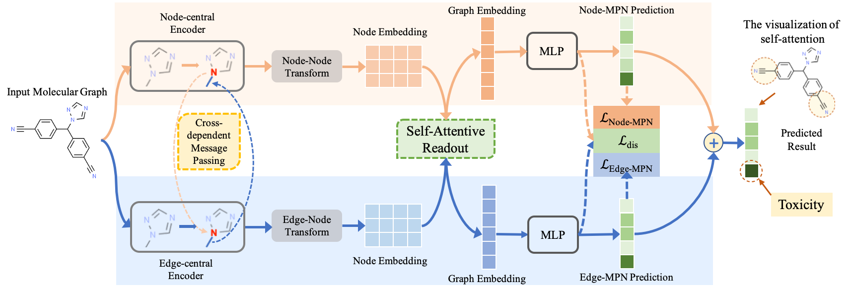
Figure 2: Overview of $\mathsf{MV}$-$\mathsf{GNN}$ models. $\mathsf{MV}$-$\mathsf{GNN}$ models pass the graph through two encoders to generate two sets of node embeddings. A shared self-attention readout learns the node importance and produce two graph embeddings accordingly. The embeddings are then fed into two MLPs to make predictions. The final prediction is the ensemble of the two predictions. Furthermore, by visualizing the learned attentions over nodes, one can identify the atoms/functional groups that are responsible for the predictions. For example, $\mathsf{MV}$-$\mathsf{GNN}$ finds out that the cyano groups contribute to the toxicity significantly.

3.1 Overview of the Multi-View Architecture

The multi-view architecture equally considers both atom features and bond features for constituting a molecular representation. As shown in Figure 2, the proposed architecture contains two concurrent sub-modules, Node-central encoder and Edge-central encoder, which output the node/edge embedding matrix from the graph topology as well as node/edge features. Next, $\mathsf{MV}$-$\mathsf{GNN}$ adopts an aggregation function to produce the graph embedding vector from the node/edge embedding matrix. Other than the mean-pooling mechanism, we propose to use the self-attentive aggregation to learn different weights of the node/edge embeddings to produce the final graph embedding. Furthermore, the self-attentive aggregation layer is shared between the node-central and edge-central encoders, to reinforce the learning of the node features and the edge features, respectively. After the self-attentive aggregation, $\mathsf{MV}$-$\mathsf{GNN}$ feeds the graph embedding from the node-central encoder and the edge-central encoder to two MLPs to fit the loss function. To stabilize the training process of this multi-view architecture, we employ the disagreement loss to enforce the outputs of the two MLPs to be close with each other.

3.2 Node-central and Edge-central Encoders

To ease the exposition, in the sequel when using one singe superscript we mean the hop index $k$ while ignoring the layer/iteration index $l$.

Node-central Encoder. $\mathsf{Node}$-$\mathsf{GNN}$ is built upon the generalized message passing in Equation 1. Additionally, we add input and output layers, to enhance its expressive power. Specifically,

$$\mathbf{m}_{v}^{{(k)}}=\text{\text{AGG}}_{\text{node}}(\{\mathbf{h}_{v}^{(k-1)},\mathbf{h}_{u}^{(k-1)},\mathbf{e}_{uv}\;|\;u\in\mathcal{N}_{v}\}),\quad\mathbf{h}_{v}^{(k)}=\text{MLP}_{\text{node}}(\{\mathbf{m}_{v}^{{(k)}},\mathbf{h}_{v}^{(0)}\}),$$ (4)

where ${\mathbf{h}}_{v}^{(0)}=\sigma({\mathbf{W}}_{\text{nin}}{\mathbf{x}}_{v})$ is the input state of $\mathsf{Node}$-$\mathsf{GNN}$, ${\mathbf{W}}_{\text{nin}}\in\mathbb{R}^{d_{\text{hid}}\times d_{n}}$ is the input weight matrix. The input layer can also be viewed as a residual connection. After $L$ iterations of message passing, we utilize an additional message passing step with a new weight matrix ${\mathbf{W}}_{\text{nout}}\in\mathbb{R}^{d_{\text{out}}\times(d_{n}+d_{\text{hid}})}$ to produce the final node embeddings:

$${\mathbf{m}}_{v}^{\text{o}} =\text{AGG}_{\text{node}}(\{{\mathbf{h}}_{u}^{(L,K_{L})},{\mathbf{x}}_{u}|u\in\mathcal{N}_{v}\}),\quad{\mathbf{h}}_{v}^{\text{o}}=\sigma({\mathbf{W}}_{\text{nout}}{\mathbf{m}}_{v}^{\text{o}}).$$ (5)

We denote ${\mathbf{H}}_{n}=[{\mathbf{h}}_{1}^{\text{o}},\cdots,{\mathbf{h}}_{p}^{\text{o}}]\in\mathbb{R}^{d_{\text{out}}\times p}$ as the output embeddings of $\mathsf{Node}$-$\mathsf{GNN}$, where $d_{\text{out}}$ is the dimension of output embeddings.

Edge-central Encoder. In classical graph theory, the line graph $L(G)$ of a graph $G$ is the graph that encodes the adjacencies between edges of $G$ [19]. $L(G)$ provides a fresh perspective to understand the original graph, i.e., the nodes are viewed as the connections while edges are viewed as entities. Therefore, it enables to perform message passing operation through edges to imitate $\mathsf{Node}$-$\mathsf{GNN}$ on $L(G)$ [62]. Namely, given an edge $(v,w)$, we can formulate the Edge-based GNN ($\mathsf{Edge}$-$\mathsf{GNN}$) as:

$${\mathbf{m}}_{vw}^{(k)} =\text{AGG}_{\text{edge}}(\{{\mathbf{h}}_{vw}^{(k-1)},{\mathbf{h}}_{uv}^{(k-1)},{\mathbf{x}}_{u}|u\in\mathcal{N}_{v}\setminus w\}),\quad{\mathbf{h}}_{vw}^{(k)}=\text{MLP}_{\text{edge}}(\{{\mathbf{m}}_{vw}^{(k-1)},{\mathbf{h}}_{vw}^{(0)}\}),$$ (6)

where ${\mathbf{h}}_{vw}^{(0)}=\sigma({\mathbf{W}}_{\text{ein}}{\mathbf{e}}_{vw})$ is the input state of $\mathsf{Edge}$-$\mathsf{GNN}$, ${\mathbf{W}}_{\text{ein}}\in\mathbb{R}^{d_{\text{hid}}\times d_{e}}$ is the input weight matrix. In Equation 6, the state vector is defined on edge $\mathbf{e}_{vw}$ and the neighboring edge set of $\mathbf{e}_{vw}$ is defined as all edges connected to the start node $v$ except the node $w$. Figure 7(b) in Appendix B shows an example of the message passing process in $\mathsf{Edge}$-$\mathsf{GNN}$.

After recurring $L$ steps of message passing, the output of $\mathsf{Edge}$-$\mathsf{GNN}$ is the state vectors for edges. In order to incorporate the shared-attentive readout to generate the graph embedding, one more round of message passing on nodes is employed to transform edge-wise embeddings to node-wise embeddings, and generate the second set of node embeddings. Specifically,

$$\text{(Edge-Node transform)}\quad{\mathbf{m}}_{v}^{\text{o}} =\text{AGG}_{\text{edge}}({\mathbf{h}}_{uv}^{(L,K_{L})},{\mathbf{x}}_{u}|u\in\mathcal{N}_{v}),\quad{\mathbf{h}}_{v}^{\text{o}}=\sigma({\mathbf{W}}_{\text{eout}}{\mathbf{m}}_{v}^{\text{o}}),$$ (7)

where ${\mathbf{W}}_{\text{eout}}\in\mathbb{R}^{d_{\text{out}}\times(d_{n}+d_{\text{hid}})}$ specifies the weight matrix. Therefore, the final output of $\mathsf{Edge}$-$\mathsf{GNN}$ provides a new set of node embeddings from the edge message passing process. This set of node embeddings are denoted as ${\mathbf{H}}_{e}=[{\mathbf{h}}_{1}^{\text{o}},\cdots,{\mathbf{h}}_{p}^{\text{o}}]\in\mathbb{R}^{d_{\text{out}}\times p}$.

3.3 Interpretable Readout Component for Generating Graph-level Embedding

To obtain a fixed length graph representation, a readout component is usually employed on the node embeddings. In this work, we considered two readout transformations to obtain the molecular representation. The first is the simple mean-pooling readout, the molecular representation is given by ${\xi}_{n}=\frac{1}{p}\sum_{{\mathbf{h}}_{i}^{o}\in{\mathbf{H}}_{n}}{\mathbf{h}}_{i}^{\text{o}}$. However, the average operation tends to produce smooth outputs. Therefore, it diminishes the expressive power. To overcome the drawbacks of mean-pooling, we develop the interpretable self-attentive readout component based on the attention mechanism [54, 27]. Namely, given an output of node-central encoder ${\mathbf{H}}_{n}\in\mathbb{R}^{d_{\text{out}}\times p}$, the self-attention ${\mathbf{S}}$ over nodes is:

$${\mathbf{S}}=\operatorname{softmax}\left({\mathbf{W}}_{2}\tanh\left({\mathbf{W}}_{1}{\mathbf{H}}_{n}\right)\right),$$ (8)

where ${\mathbf{W}}_{1}\in\mathbb{R}^{d_{\text{attn}}\times d_{\text{out}}}$ and ${\mathbf{W}}_{2}\in\mathbb{R}^{r\times d_{\text{attn}}}$ are learnable matrices. In Equation 8, ${\mathbf{W}}_{1}$ linearly transforms the node embeddings from $d_{\text{out}}$-dimensional space to a $h_{\text{attn}}$-dimensional space. ${\mathbf{W}}_{2}$ provides $r$ different insights of node importance, then followed by a softmax function to normalize the importance. To enable the feature information extracted from node and edge encoders communicating during the multi-view training process, we share the parameters ${\mathbf{W}}_{1}$ and ${\mathbf{W}}_{2}$ between the two sub-models. Given ${\mathbf{S}}$, we can obtain the graph-level embedding by $\bm{\xi}_{n}={\mathsf{Flatten}}({\mathbf{S}}{\mathbf{H}}_{n}^{\top})$. The self-attention ${\mathbf{S}}$ implies importance of the nodes when generating graph embedding, hence indicating contributions of the nodes for downstream tasks, which equips $\mathsf{MV}$-$\mathsf{GNN}$ with interpretability power.

3.4 The Disagreement Loss for $\mathsf{MV}$-$\mathsf{GNN}$ Models

Suppose the dataset contains graphs $\mathcal{G}=\{G_{i}\}_{i=1}^{K}$ and corresponding labels $\mathcal{Y}=\{{\mathbf{y}}_{i}\}_{i=1}^{K}$. Given one graph $G_{i}$, due to the nature of the multi-view architecture, we obtain two graph embeddings $\bm{\xi}_{n}$ and $\bm{\xi}_{e}$, from the node message passing and edge message passing, respectively. Feeding them into the MLPs results in two predictions $\bm{\gamma}_{n,i}$ and $\bm{\gamma}_{e,i}$ for the same target $\mathbf{y}_{i}$. Naturally, the losses should get the supervised prediction loss involved, i.e., $\mathcal{L}_{\text{pred}}=\sum_{G_{i}\in\mathcal{G}}(\mathcal{L}_{{\mathsf{Node}}\text{-}{\mathsf{GNN}}}({\mathbf{y}}_{i},\bm{\gamma}_{n,i})+\mathcal{L}_{{\mathsf{Edge}}\text{-}{\mathsf{GNN}}}({\mathbf{y}}_{i},\bm{\gamma}_{e,i}))$. The specific loss function $\mathcal{L}_{{\mathsf{Node}}\text{-}{\mathsf{GNN}}}$ and $\mathcal{L}_{{\mathsf{Edge}}\text{-}{\mathsf{GNN}}}$ should depend on the task types, say, cross-entropy for classification and mean squared error for regression.

However, with only the $\mathcal{L}_{\text{pred}}$ loss, we observed unstable behaviors of the training process, which is caused by the loose constraint of the node and edge message passings. To resolve this problem, we propose the disagreement loss, which is responsible for restraining the two predictions from node-central and edge-central encoders. Specifically, we employ the mean squared error $\mathcal{L}_{\text{dis}}=\sum_{G_{i}\in\mathcal{G}}\left|\gamma_{n,i}-\gamma_{e,i}\right|^{2}$. Overall, the shared self-attentive readout and the disagreement loss alleviate the node variant dependency, and reinforce the restriction during the training process to promise the model converge to a stationary status. Finally, the overall loss function contains two parts: $\mathcal{L}=\mathcal{L}_{\text{pred}}+\lambda\mathcal{L}_{\text{dis}}$, where $\lambda$ is a tradeoff hyper-parameter.

3.5 $\mathsf{MV}$-${\mathsf{GNN^{cross}}}$: $\mathsf{MV}$-$\mathsf{GNN}$ Equipped with the Cross-dependent Message Passing Scheme

Though $\mathsf{MV}$-$\mathsf{GNN}$ is proved to have superior performance for many molecular property prediction tasks (as verified in the experiments), we find that the information flow in $\mathsf{MV}$-$\mathsf{GNN}$ is not sufficiently efficient. Suppose all the information needed to predict the property resides in the molecule itself. For $\mathsf{MV}$-$\mathsf{GNN}$, the information flows through two distinct paths in parallel: one path is the $\mathsf{Node}$-$\mathsf{GNN}$ encoder, the other one is the $\mathsf{Edge}$-$\mathsf{GNN}$ encoder. The information from the two paths finally joins at the disagreement loss.

However, the two flows of information could meet earlier, to enable more efficient information communication. The strategy to implement this is the cross-dependent message passing scheme. On a high level, it makes the message passing operations of the node and edge cross-dependent with each other. Specifically, we change the message passing operations of the node and edge encoders (in Equations (4) and (6), respectively) to be:

$${\mathbf{m}}_{v}^{(k)} =\text{AGG}_{\text{node}}(\{{\mathbf{h}}_{v}^{(k-1)},{\mathbf{h}}_{u}^{(k-1)},{\color[rgb]{0,0,1}{\mathbf{h}}_{vu}^{(k-1)}},{\mathbf{e}}_{vu}|u\in\mathcal{N}_{v}\}),\;\mathbf{h}_{v}^{(k)}=\text{MLP}_{\text{node}}(\{\mathbf{m}_{v}^{{(k)}},\mathbf{h}_{v}^{(0)}\}),$$ (9)

$${\mathbf{m}}_{vw}^{(k)} =\text{AGG}_{\text{edge}}(\{{\mathbf{h}}_{vw}^{(k-1)},{\mathbf{h}}_{uv}^{(k-1)},{\color[rgb]{0,0,1}{\mathbf{h}}_{u}^{(k-1)}},{\mathbf{x}}_{u}|u\in\mathcal{N}_{v}\setminus w\}),\;{\mathbf{h}}_{vw}^{(k)}=\text{MLP}_{\text{edge}}(\{{\mathbf{m}}_{vw}^{(k)},{\mathbf{h}}_{vw}^{(0)}\}).$$

The first row indicates new node message passing, while the second row shows edge message passing. One can see that when applying aggregation in node message passing, we use the newest hidden states of edges (blue colored). While conducting aggregation in edge message passing, it requires the newest hidden states of nodes. In this way, the two paths of information flow become cross-dependent with each other. We will empirically show that the cross-dependent message passing scheme enables more expressive power compared to the vanilla $\mathsf{MV}$-$\mathsf{GNN}$ architecture.

3.6 Expressive Power of $\mathsf{MV}$-$\mathsf{GNN}$ and $\mathsf{MV}$-${\mathsf{GNN^{cross}}}$

$\mathsf{MV}$-$\mathsf{GNN}$ and $\mathsf{MV}$-${\mathsf{GNN^{cross}}}$ achieve superior performance compared to all baselines in the experiments. In this section, we justify its performance by studying their expressiveness under the framework of distinguishing non-isomorphic graphs. By comparing the expressive power with the well justified architecture GIN [60], we reach the following conclusions.

Proposition 1.

In terms of expressive power of models, the following conclusions hold:

1. $\mathsf{MV}$-$\mathsf{GNN}$ is at least as powerful as the Graph Isomorphism Network (GIN of [60]), which provably generalizes the WL graph isomorphism test.

2. $\mathsf{MV}$-${\mathsf{GNN^{cross}}}$ is strictly more powerful than the Graph Isomorphism Network.

Detailed proof is deferred to Appendix C. Proposition 1 shows that $\mathsf{MV}$-$\mathsf{GNN}$ models have sufficient model capacity in terms of distinguishing graphs compared to the GIN architecture and the WL graph isomorphism test. This observation also explains why it reaches superior performance on various baseline tasks, which will be further verified in the experiments.

4 Experimental Results

We conduct the performance evaluations of $\mathsf{MV}$-$\mathsf{GNN}$ and $\mathsf{MV}$-${\mathsf{GNN^{cross}}}$ with various SOTA baselines on molecular property classification and regression tasks. Due to the space limitation, the results of the regression tasks are deferred to Section E.6. We also preform the ablation studies on different components of the $\mathsf{MV}$-$\mathsf{GNN}$ models. Lastly, we conduct case studies to demonstrate the interpretability power of the proposed models. Source code will be released soon.

Datasets. We experimented with 11 popular benchmark datasets, among which six are classification tasks and the others are regression tasks. Specifically, BACE is about the biophysics property; BBBP, Tox21, Toxcast, SIDER, and Clintox record several molecular physiology properties; QM7 and QM8 contain molecular quantum mechanics information; ESOL, Lipophilicity and Freesolv document physical chemistry properties [58]. Details are deferred to Section E.1.

Baselines. We thoroughly evaluate the performance of our methods against popular baselines from both machine learning and chemistry communities. Among them, Influence Relevance Voting ($\mathsf{IRV}$) [52], $\mathsf{LogReg}$ [11], Random Forest ($\mathsf{RF}$/$\mathsf{RF\_Reg}$) [6] utilize different traditional machine learning approaches. $\mathsf{GraphConv}$ [9], $\mathsf{Weave}$ [22], $\mathsf{SchNet}$ [47], $\mathsf{MGCN}$ [30], $\mathsf{N}$-$\mathsf{Gram}$ [29], $\mathsf{MPNN}$ [15] and $\mathsf{DMPNN}$ [62] are GNN-based models. For $\mathsf{SchNet}$ and $\mathsf{MGCN}$, we use DGL [55] implementations; for $\mathsf{N}$-$\mathsf{Gram}$ and $\mathsf{DMPNN}$, we use open source codes provided by the author; for $\mathsf{MPNN}$, we use the implementation by [62]; for others, we use the MoleculeNet [58] implementations. Details can be found in Section E.2.

Dataset Splitting. We apply the scaffold splitting for all tasks on all datasets, which is more practical and challenging than random splitting. More details about this splitting method is introduced in Section E.1. Evaluation Metrics. All classification task are evaluated by AUC-ROC. For the regression task, we apply MAE and RMSE to evaluate the performance of regression task on different datasets.

4.1 Performance Evaluation on Classification Tasks

To demonstrate the effectiveness of shared self-attentive readout and the disagreement loss, we also implement two naive schemes. $\mathsf{Concat+Mean}$ concatenates the mean-pooling outputs of the two sub-modules, and $\mathsf{Concat+Attn}$ concatenates the self-attentive outputs of the two sub-modules. Table 1 summarizes the results of the classification tasks. To evaluate the robustness of our method, we report the mean and standard deviation of 10 times runs with different random seeds for $\mathsf{MV}$-$\mathsf{GNN}$, $\mathsf{MV}$-${\mathsf{GNN^{cross}}}$ and the variants. Table 1 implies the following observations: (1) our $\mathsf{MV}$-$\mathsf{GNN}$ models gain significant enhancement against SOTAs on all datasets consistently, $\mathsf{MV}$-${\mathsf{GNN^{cross}}}$ even performs slightly better than $\mathsf{MV}$-$\mathsf{GNN}$. Specifically, $\mathsf{MV}$-$\mathsf{GNN}$ gains the average AUC boost by $1.15\%$ on average compared with the SOTAs on each dataset, while $\mathsf{MV}$-${\mathsf{GNN^{cross}}}$ improves it to $1.65\%$, which is regarded as the remarkable boost, considering the challenges on these benchmarks. (2) Compared with the SOTAs, $\mathsf{MV}$-$\mathsf{GNN}$ and $\mathsf{MV}$-${\mathsf{GNN^{cross}}}$ has much smaller standard deviation, which implies that our models are more robust than the baselines. (3) Compared with the two simple variants, $\mathsf{MV}$-$\mathsf{GNN}$ and $\mathsf{MV}$-${\mathsf{GNN^{cross}}}$ demonstrate the superiority both on performance and robustness. It validates the effectiveness of the multi-view architecture with disagreement loss constraint.

Table 1: Performance of classification tasks on AUC-ROC (higher is better) with the scaffold split. Best score is marked as bold, and the best baseline is marked in gray. Green cells indicate the results of our methods.

Method	BACE	BBBP	Tox21	ToxCast	SIDER	ClinTox
$\mathsf{IRV}$	0.838±0.055	0.877±0.051	0.699±0.055	0.604±0.037	0.595±0.022	0.741±0.069
$\mathsf{LogReg}$	0.844±0.040	0.835±0.067	0.702±0.028	0.613±0.033	0.583±0.034	0.733±0.084
RF	0.856±0.019	0.881±0.050	0.744±0.051	0.582±0.049	0.622±0.042	0.712±0.066
$\mathsf{GraphConv}$	0.854±0.011	0.877±0.036	0.772±0.041	0.650±0.025	0.593±0.035	0.845±0.051
$\mathsf{Weave}$	0.791±0.008	0.837±0.065	0.741±0.044	0.678±0.024	0.543±0.034	0.823±0.023
$\mathsf{SchNet}$	0.750±0.033	0.847±0.024	0.767±0.025	0.679±0.021	0.545±0.038	0.717±0.042
$\mathsf{MGCN}$	0.734±0.030	0.850±0.064	0.707±0.016	0.663±0.009	0.552±0.018	0.634±0.042
$\mathsf{N}$-$\mathsf{Gram}$	0.876±0.035	0.912±0.013	0.769±0.027	$-$	0.632±0.005	0.855±0.037
$\mathsf{MPNN}$	0.815±0.044	0.913±0.041	0.808±0.024	0.691±0.013	0.595±0.030	0.879±0.054
$\mathsf{DMPNN}$	0.852±0.053	0.919±0.030	0.826±0.023	0.718±0.011	0.632±0.023	0.897±0.040
$\mathsf{Concat+Mean}$	0.842±0.004	0.930±0.002	0.816±0.003	0.721±0.001	0.621±0.007	0.882±0.008
$\mathsf{Concat+Attn}$	0.832±0.007	0.931±0.006	0.819±0.003	0.728±0.002	0.632±0.008	0.913±0.009
$\mathsf{MV}$-$\mathsf{GNN}$	0.863±0.002	0.938±0.003	0.833±0.001	0.729±0.006	0.644±0.003	0.930±0.003
$\mathsf{MV}$-${\mathsf{GNN^{cross}}}$	0.892±0.011	0.933±0.006	0.836±0.006	0.744±0.005	0.639±0.012	0.923±0.007

4.2 Ablation Studies on Key Design Choices

This section focuses on the impacts of three key components in the proposed $\mathsf{MV}$-$\mathsf{GNN}$ models: the disagreement loss, the shared self-attentive readout and the cross-dependent message passing scheme. We report the results of three datasets with fixed train/valid/test sets to evaluate the impacts in Table LABEL:tab:ablationstudy, which demonstrates the proposed multi-view models overall performs the best on all three datasets. Moreover, we find that both attention and disagreement loss can boost the performance compared with “No All” method. Particularly, when the self-attention mechanism is employed, the performance has already surpassed all the baseline models including $\mathsf{MPNN}$ and $\mathsf{DMPNN}$, which proves that the molecular property is affected by the various atoms differently. Hence, the weights of atoms should not be considered equivalently. Overall, the proposed $\mathsf{MV}$-$\mathsf{GNN}$ models that adopts both disagreement loss and self-attention outperforms the other variants, indicating that the combination of them would significantly facilitate the model training.

Figure 3: Ablation study on the variants of $\mathsf{MV}$-$\mathsf{GNN}$.

	ToxCast	SIDER	ClinTox
No All	0.718	0.644	0.852
Only Attention	0.728	0.646	0.901
Only Disagreement Loss	0.722	0.648	0.863
$\mathsf{MV}$-$\mathsf{GNN}$	0.731	0.652	0.907
$\mathsf{MV}$-${\mathsf{GNN^{cross}}}$	0.744	0.639	0.923

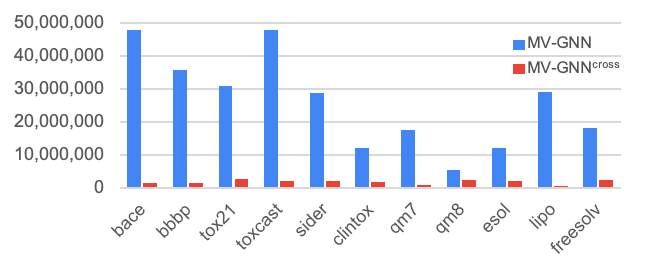
Figure 4: Model parameters comparison.

Effect of cross-dependent message passing. We plot the number of parameters in $\mathsf{MV}$-$\mathsf{GNN}$ and $\mathsf{MV}$-${\mathsf{GNN^{cross}}}$ in Figure 4. It clearly indicates that $\mathsf{MV}$-${\mathsf{GNN^{cross}}}$, while enjoying competitive performance, needs much less amount of parameters than $\mathsf{MV}$-${\mathsf{GNN^{cross}}}$. Specifically, the average number of parameters of $\mathsf{MV}$-$\mathsf{GNN}$ is 15.26 times of that of $\mathsf{MV}$-${\mathsf{GNN^{cross}}}$. This confirms that the cross-dependent message passing scheme can significantly improve the expressive power of the model, by enabling a more efficient information communication scheme in the multi-view architecture.

4.3 Case Study: Visualization of Interpretability Results

To illustrate the interpretability power of $\mathsf{MV}$-$\mathsf{GNN}$, we visualize certain molecules with the learned attention weights of $\mathsf{MV}$-$\mathsf{GNN}$ associated with each atom within one molecule from the Clintox dataset, with toxicity as the labels. Figure 5 instantiates the graph structures of the molecules along with the corresponding atom attentions. The attention values lower than 0.01 are omitted. We observe that different atoms indeed react distinctively: 1) Most carbon (C) atoms that are responsible for constructing the molecule topology have got zero attention value. It is because these kinds of sub-structures usually do not affect the toxicity of a compound. 2) Beyond that, $\mathsf{MV}$-$\mathsf{GNN}$ promotes the learning of the functional groups with impression on molecular toxicity, e.g., toxic functional group trifluoromethyl and cyanide are known responsible for the toxicity [45], which reveal extremely high attention value in Figure 5. These high attention values can be used to explain the toxicity of the molecules. Compared with the previous models, $\mathsf{MV}$-$\mathsf{GNN}$ is able to provide reasonable interpretability results for the predictions, which is crucial for the real drug discovery.

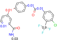
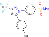
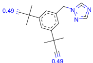
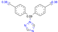
Figure 5: Visualization of attention values on ClinTox data. Attention value smaller than 0.01 is omitted. Different color indicates different elements: black: C, blue: N, red: O, green: Cl, yellow: S, sky-blue: F. First two molecules: the molecules with trifluoromethyl. Last two molecules: the molecules with cyanide.

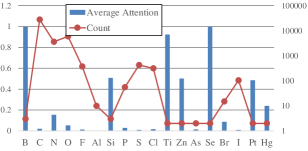
Figure 6: Statistics of attentions in ClinTox. Left axis: the average attention value of the element. Right axis: the count of the element.

Furthermore, we provide a comprehensive statistics of the attention values over the entire ClinTox dataset. Figure 6 demonstrates the average attention values and the total occurrences of each element. It is notable that, 1) atoms with high frequency do not receive high attention. For example, atom C is an essential element to maintain the molecular topology, yet it does not have significant impact on the toxicity. 2) atoms with low frequency but high attention values are generally heavy elements. For example, $\mathsf{Hg}$ (Mercury) is widely known by its toxicity. The accompanied attention value of $\mathsf{Hg}$ is relevantly high because it usually affects the toxic property greatly. Overall, the case study shows that the proposed $\mathsf{MV}$-$\mathsf{GNN}$ models are able to provide reasonable interpretability for the prediction results.

5 Brief Related Work

Molecular representation learning and GNNs are extensively studied, which renders it very difficult comprehensively surveying all previous work. Here we only summarize some of the most related ones, and leave details in Appendix A. How to get accurate molecular representation is vital for molecular property prediction. Traditionally, chemical experts design a so-called molecular fingerprint manually based on their domain knowledge, e.g., ECFP [42]. Several studies have exploited the deep learning approaches to improve the molecular representation. One perspective is to take advantage of the molecular SMILES representation [56]. Based on the SMILES, [61, 21] apply RNN-based models to generate the molecular fingerprint. Another promising perspective is to explore the graph structure of a molecule by graph neural networks (GNNs), which has attracted a surge of interest recently [46, 22, 48, 47, 29, 60, 44, 59, 54, 15, 62, 24, 30]. In this line of work various GNN-based models have been proposed for generating molecular representations [9, 1, 48, 47, 29], e.g., [9] applies convolutional networks on the molecular graphs to generate molecular fingerprint.

6 Conclusions

We propose multi-view graph neural networks ($\mathsf{MV}$-$\mathsf{GNN}$ and $\mathsf{MV}$-${\mathsf{GNN^{cross}}}$) for molecular property prediction. Unlike previous attempts focusing exclusively on either atom-oriented graph structures or bond-oriented graph structures, our method, inspired by multi-view learning, takes both atom and bond information into consideration. We develop several techniques for the multi-view architecture: a shared self-attentive attention scheme enabling the interpretability power; a disagreement loss to restrain the distance between the outputs of the two views; a cross-dependent message passing scheme to enhance information communication between the views. Extensive experiments against SOTA models demonstrate that $\mathsf{MV}$-$\mathsf{GNN}$ and $\mathsf{MV}$-${\mathsf{GNN^{cross}}}$ outperform all baselines significantly, as well as equip with strong robustness.

Appendix A Related Work in Details

The most crucial part of addressing molecular property prediction problem is to get an accurate vector representation of the molecules. Relevant studies can be categorized into three aspects: hand-crafted molecular fingerprints based methods, SMILES sequence based techniques, and graph structure based techniques.

Hand-crafted molecular fingerprints based methods. The traditional feature extraction method enlists experts to design molecular fingerprints manually, based on biological experiments and chemical knowledge [35], such as the property of molecular sub-structures. These types of fingerprint methods generally work well for particular tasks but lack universality. One representative approach is called circular fingerprints [16]. Circular fingerprints employ a fixed hash function to extract each layer’s features of a molecule based on the concatenated features of the neighborhood in the previous layer. Extended-Connectivity Fingerprint (ECFP) [42] is one of the most famous examples of hash-based fingerprints. The generated fingerprint representations usually go through machine learning models to perform further predictions, such as Logistic Regression [23], Random Forest [6], and Influence Relevance Voting (IRV) [52]. Nonetheless, this type of hand-crafted fingerprint has a notable problem: since the characteristic of the hash function is non-invertible, it might not be able to catch enough information when being converted.

SMILES sequence based techniques. SMILES sequence based models, such as Seq2seq Fingerprint [61], spot the potentially useful information of the molecular SMILES sequence data by adequately training them using Recurrent Neural Networks (RNNs), in order to obtain the vector representation of the molecule. These vectors then go through other supervised models to perform property prediction, e.g., GradientBoost [12]. The SMILES-based models are inspired by the sequence learning in Natural Language Processing [5], which takes an unlabeled dataset as the input to convert a SMILES to a fingerprint, then recovers the fingerprint back to a sequence representation for better learning.

Graph structure based techniques. A molecule could be represented as a graph based on its chemical structure, e.g., consider the atoms as the nodes, and the chemical bonds between the atoms as the edges. Thus, many graph theoretic algorithms could be applied to represent a molecule by embedding the graph features into a continuous vector [58, 28, 49]. A noted study proposed the idea of neural fingerprints, which applies convolutional neural networks on graphs directly [9]. The difference between neural fingerprints and circular fingerprints is the replacement of the hash function. Neural fingerprints apply a non-linear activated densely connected layer to generate the fingerprints. These kind of deep Graph Convolutional Neural Networks are established by learning a function on the graph node features and the graph structure matrix representation [10, 28]. Other graph-based models such as the Weave model have also been proposed [22]. The Weave model is another graph-based convolutional model. The key difference between the Weave model and neural fingerprints [9] is the updating procedure of the atom features. It combines all the atoms in a molecule with their matching pairs instead of the neighbors of the atoms. More relevant research that focus on exploiting the molecular graphs with graph convolutional network have been studied recently, e.g., [48, 47] have involved the 3D information of the molecules to help exploit the molecular graph structure. Other attempts such as [44, 59] turn to develop aggregation weights learning schemes based on the prior knowledge of Graph Attention Network [54]. Moreover, [15] proposes a framework to implement message passing process between each atom to form a molecular representation. Inspired by this work, [62, 24] convert the passing process to bond-wise instead of atom-wise. [30] introduces multilevel graph structures based on the interactions between atom-pairs.

Appendix B More Details on $\mathsf{MV}$-$\mathsf{GNN}$ Models

$\mathsf{MV}$-$\mathsf{GNN}$ models establish two sub-modules, $\mathsf{Node}$-$\mathsf{GNN}$ and $\mathsf{Edge}$-$\mathsf{GNN}$. The process for each module can be categorized into three phases: neighbor aggregation, attached features collection, and message update. As shown in Figure 7(a), for the $\mathsf{Node}$-$\mathsf{GNN}$ module, taking node $v_{3}$ as an example: 1) neighbor nodes aggregation: aggregating the node features of its neighbor nodes $v_{2}$, $v_{4}$ and $v_{5}$; 2) getting the initial edge features as the attached features from the connected edge $\bm{e}_{23}$, ${\mathbf{e}}_{34}$, and $\mathbf{e}_{35}$; 3) updating the state of $v_{3}$ using Equation 4.

Figure 7(b) demonstrates the edge message construction in the $\mathsf{Edge}$-$\mathsf{GNN}$ module. Take edge $\mathbf{e}_{35}$ as an example. 1) neighbor edges aggregation: aggregating the edge features of its neighbor edges, edge $\mathbf{e}_{23}$, edge $\mathbf{e}_{43}$; 2) getting the initial node information as the attached features from the endpoint node $v_{2}$ of edge $\mathbf{e}_{23}$, node $v_{4}$ of $\mathbf{e}_{43}$ ; 3) updating the message of $\mathbf{e}_{35}$ using Equation 6.

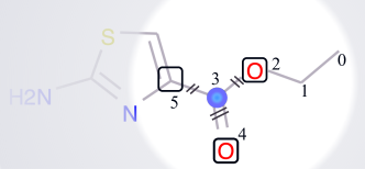
(a) $\mathsf{Node}$-$\mathsf{GNN}$ message passing

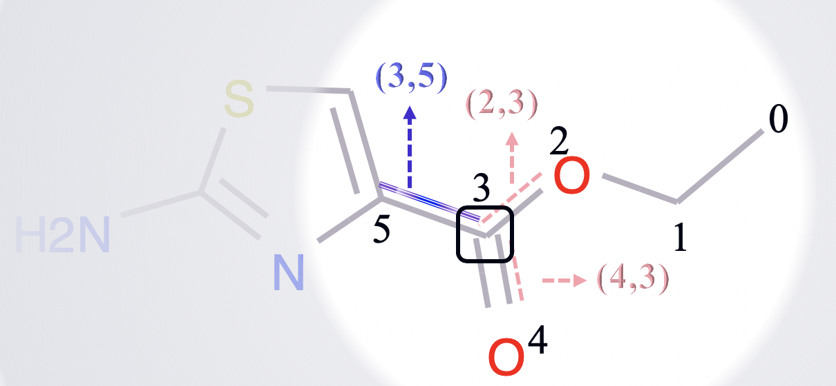
(b) $\mathsf{Edge}$-$\mathsf{GNN}$ message passing

Figure 7: Examples of the message passing phase in $\mathsf{Node}$-$\mathsf{GNN}$ (Figure 7(a)) and $\mathsf{Edge}$-$\mathsf{GNN}$ (Figure 7(b)).

Appendix C Proof of Expressive Power

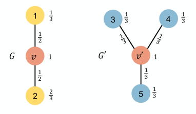
Figure 8: Example of the two subgraph structures.

Proof of Proposition 1.

Firstly we show that $\mathsf{MV}$-$\mathsf{GNN}$ is at least as powerful as the Graph Isomorphism Network (GIN of xu2018powerful [60]). $\mathsf{MV}$-$\mathsf{GNN}$ involves both node message passing and edge message passing processes, which constitutes the two-view information flows. Suppose that one blocks the information flowing in the edge passing, say, by setting the initial hidden states of all edges to be $0$. At this moment, if one takes the the sum aggregation in xu2018powerful [60] as the specific realization of the aggregation operation, then $\mathsf{MV}$-$\mathsf{GNN}$ recovers the GIN architecture. So we can conclude that $\mathsf{MV}$-$\mathsf{GNN}$ has at least the same expressive power as GIN.

Then we prove that $\mathsf{MV}$-${\mathsf{GNN^{cross}}}$ is strictly more powerful than GIN. In order to illustrate this, we construct specific graph examples such that one iteration of message passing in GIN cannot distinguish the nodes with different subgraph structures. However, $\mathsf{MV}$-${\mathsf{GNN^{cross}}}$ with the cross-dependent message passing scheme is able to discriminate the two nodes. To enable fair comparison, we assume that both GIN and $\mathsf{MV}$-${\mathsf{GNN^{cross}}}$ use the same aggregation function as in the GIN paper [60]. That is, we use the sum aggregation with a parameter $\epsilon^{(l)}$, i.e., $\text{AGG}^{(l)}(\{\mathbf{h}_{v}^{(l,k-1)},\mathbf{h}_{u}^{(l,k-1)},\mathbf{e}_{uv}|u\in\mathcal{N}_{v}\})=((1+\epsilon^{(l)})\mathbf{h}_{v}^{(l,k-1)}+\sum_{u\in\mathcal{N}_{v}}\mathbf{h}_{u}^{(l,k-1)})||(\sum_{u\in\mathcal{N}_{v}}\mathbf{e}_{uv})$ ($||$ is the concatenation operation).

Assume there are two graphs $G,G^{\prime}$ as shown in Figure 8. The two nodes therein, $v$ and $v^{\prime}$ have different local subgraph structures. For simplicity, let all the initial node features, edge features and hidden states have dimensionality as 1. Specifically, for node features and hidden states, we have $\mathbf{h}_{v}=\mathbf{x}_{v}=1$, $\mathbf{h}_{v^{\prime}}=\mathbf{x}_{v^{\prime}}=1$, $\mathbf{h}_{1}=\mathbf{x}_{1}=\frac{1}{3}$, $\mathbf{h}_{2}=\mathbf{x}_{2}=\frac{2}{3}$, $\mathbf{h}_{3}=\mathbf{h}_{4}=\mathbf{h}_{5}=\mathbf{x}_{3}=\mathbf{x}_{4}=\mathbf{x}_{5}=\frac{1}{3}$. For edge features and hidden states, one has $\mathbf{h}_{v1}=\mathbf{h}_{1v}=\mathbf{e}_{v1}=\frac{1}{2}$, $\mathbf{h}_{v2}=\mathbf{h}_{2v}=\mathbf{e}_{v2}=\frac{1}{2}$, $\mathbf{h}_{v^{\prime}3}=\mathbf{h}_{3v^{\prime}}=\mathbf{e}_{v^{\prime}3}=\frac{1}{3}$, $\mathbf{h}_{v^{\prime}4}=\mathbf{h}_{4v^{\prime}}=\mathbf{e}_{v^{\prime}4}=\frac{1}{3}$, $\mathbf{h}_{v^{\prime}5}=\mathbf{h}_{5v^{\prime}}=\mathbf{e}_{v^{\prime}5}=\frac{1}{3}$.

Under this setup, we can run one iteration of message passing by hand. Specifically,

— For GIN, suppose its generalized version considers also the initial features. Then the message of node $v$ is $\mathbf{m}_{v}=(2+\epsilon,1)$, where the first dimension indicates aggregated node hidden states, the second dimension indicates aggregated edge initial features. The message of node $v^{\prime}$ is $\mathbf{m}_{v^{\prime}}=(2+\epsilon,1)$ as well. Since the state update function is injective, after the state update, the hidden states of node $v$ and $v^{\prime}$ will become the same, thus indistinguishable.

— For $\mathsf{MV}$-${\mathsf{GNN^{cross}}}$, one complete iteration of message passing contains one edge message passing and one node message passing. Without loss of generality, let us take it as edge message passing followed by a node message passing.

Consider edge message passing firstly. The edge messages for graph $G$ are: $\mathbf{m}_{v2}=(\overbrace{1/3}^{\text{node states sum}},\overbrace{1+\epsilon/2}^{\text{edge states sum}},\overbrace{1/3}^{\text{node features sum}})$, $\mathbf{m}_{v1}=(\overbrace{2/3}^{\text{node states sum}},\overbrace{1+\epsilon/2}^{\text{edge states sum}},\overbrace{2/3}^{\text{node features sum}})$. The two messages are different, the injective state update function will map them into different new states, suppose w.l.o.g. the new states are $\mathbf{h}_{v2}=1,\mathbf{h}_{v2}=2$.

The edge messages for graph $G^{\prime}$ are: $\mathbf{m}_{v^{\prime}3}=\mathbf{m}_{v^{\prime}4}=\mathbf{m}_{v^{\prime}5}=(\overbrace{2/3}^{\text{node states sum}},\overbrace{1+\epsilon/3}^{\text{edge states sum}},\overbrace{2/3}^{\text{node features sum}})$. They will be mapped to the same new states, assume they are $\mathbf{h}_{v^{\prime}3}=\mathbf{h}_{v^{\prime}4}=\mathbf{h}_{v^{\prime}5}=2/3$.

Then consider node message passing with the newest edge hidden states. $\mathbf{m}_{v}=(\overbrace{2+\epsilon}^{\text{node states sum}},\overbrace{3}^{\text{edge states sum}},\overbrace{1}^{\text{edge features sum}})$, $\mathbf{m}_{v^{\prime}}=(\overbrace{2+\epsilon}^{\text{node states sum}},\overbrace{2}^{\text{edge states sum}},\overbrace{1}^{\text{edge features sum}})$.

Now we have different messages for nodes $v$ and $v^{\prime}$, so it will be mapped to different new hidden states by the injective multi-layer perceptron (MLP). Thus the two nodes become distinguishable under the cross-dependent message passing scheme of $\mathsf{MV}$-${\mathsf{GNN^{cross}}}$.

∎

Appendix D The Node/Edge Feature Extraction of the Molecules

The node/edge feature extraction contains two parts: 1) node/edge messages, which are constructed by aggregating neighboring nodes/edges features iteratively; 2) molecule-level features, which are the additional molecule-level features generated by RDKit to capture the global molecular information. It consists of 200 features for each molecule [26]. Since we focus on the model architecture part, we follow the exact same protocol of [62] for the initial node (atom) and edge (bond) features selection, as well as the 200 RDKit features generation procedure. The atom features description and size are listed in Table 2, and the bond features are documented in Table 3. The RDKit features are concatenated with the node/edge embedding, to go through the final MLP to make the predictions.

Table 2: Atom features [62].

features	size	description
atom type	100	type of atom (e.g., C, N, O), by atomic number
formal charge	5	integer electronic charge assigned to atom
number of bonds	6	number of bonds the atom is involved in
chirality	4	Unspecified, tetrahedral CW/CCW, or other.
number of H	5	number of bonded hydrogen atoms
atomic mass	1	mass of the atom, divided by 100
aromaticity	1	whether this atom is part of an aromatic system
hybridization	5	sp, sp2, sp3, sp3d, or sp3d2

Table 3: Bond features [62].

features	size	description
bond type	4	single, double, triple, or aromatic
stereo	6	none, any, E/Z or cis/trans
in ring	1	whether the bond is part of a ring
conjugated	1	whether the bond is conjugated

Appendix E Experimental Setup and Additional Results

E.1 Description of Dataset

Table 4 summaries the dataset statistics [58], including the property category, number of tasks and evaluation metrics of all datasets. Six datasets are used for classification, and five datasets for regression. Noted, ToxCast contains 617 tasks, which makes it extremely time consuming to apply $\mathsf{N}$-$\mathsf{Gram}$ model, since $\mathsf{N}$-$\mathsf{Gram}$ requires task-based preprocess.

Table 4: Datasets statstics.

Category	Dataset	Task	# Tasks	# Graphs/Molecules	Metric
Biophysics	BACE	Classification	1	1513	AUC-ROC
Physiology	BBBP	Classification	1	2039	AUC-ROC
	Tox21	Classification	12	7831	AUC-ROC
	ToxCast	Classification	617	8576	AUC-ROC
	SIDER	Classification	27	1427	AUC-ROC
	ClinTox	Classification	2	1478	AUC-ROC
Quantum Mechanics	QM7	Regression	1	6830	MAE
	QM8	Regression	12	21786	MAE
Physical Chemistry	ESOL	Regression	1	1128	RMSE
	Lipophilicity	Regression	1	4200	RMSE
	FreeSolv	Regression	1	642	RMSE

Molecular Classification Datasets.

BACE dataset is collected for recording compounds which could act as the inhibitors of human $\beta$-secretase 1 (BACE-1) in the past few years [50]. The Blood-brain barrier penetration (BBBP) dataset contains the records of whether a compound carries the permeability property of penetrating the blood-brain barrier [32]. Tox21 and ToxCast [41] datasets include multiple toxicity labels over thousands of compounds by running high-throughput screening test on thousands of chemicals . SIDER documents marketed drug along with its adverse drug reactions, also known as the Side Effect Resource [25]. ClinTox dataset compares drugs approved through FDA and drugs eliminated due to the toxicity during clinical trials [14].

Molecular Regression Datasets.

QM7 dataset is a subset of GDB-13, which records the computed atomization energies of stable and synthetically accessible organic molecules, such as HOMO/LUMO, atomization energy, etc. It contains various molecular structures such as triple bonds, cycles, amide, epoxy, etc [4]. QM8 dataset contains computer-generated quantum mechanical properties, e.g., electronic spectra and excited state energy of small molecules [40]. Both QM7 and QM8 contain 3D coordinates of the molecules along with the molecular SMILES. ESOL documents the solubility of compounds [8]. Lipophilicity dataset is selected from ChEMBL database, which is an important property that affects the molecular membrane permeability and solubility. The data is obtained via octanol/water distribution coefficient experiments [13]. FreeSolv dataset is selected from the Free Solvation Database, which contains the hydration free energy of small molecules in water from both experiments and alchemical free energy calculations [33].

Dataset Splitting and Experimental Setting. We apply the scaffold splitting for all tasks on all datasets, which is more practical and challenging than random splitting. Random splitting is a common process to split the dataset into train, validation and test set randomly. However, it does not simulate the real-world scenarios for evaluating molecule-related machine learning methods [2]. Scaffold splitting splits the molecules with distinct two-dimensional structural frameworks into different subsets [2], e.g. molecules with benzene ring would be split into one subset, which could be the train/validation/test set. This means that the validation/test dataset might contain molecules with unseen structures from the training dataset, which makes the learning much more difficult. Yet, it is more difficult for the learning algorithm to accomplish satisfactory performance, but from the chemistry perspective, it is more meaningful and consequential for molecular property prediction. To alleviate the effects of randomness and over-fitting, as well as to boost the robustness of the experiments, we apply cross-validation on all the experiments. All of our experiments run 10 randomly-seeded 8:1:1 data splits, which follows the same protocols of [62].

E.2 Baselines

We thoroughly evaluate the performance of our methods with several popular baselines from both machine learning and chemistry communities. The post-fix ${\mathsf{Reg}}$ indicates the method for the regression task. Among them, Influence Relevance Voting ($\mathsf{IRV}$) is a K-Nearest Neighbor classifier, which assumes similar sub-structures reveal similar functionality [52]. $\mathsf{LogReg}$ [11] predicts the binary label by learning the coefficient combination of a logistic function based on the input features. Random Forest ($\mathsf{RF}$/$\mathsf{RF\_Reg}$) [6] is a decision tree based ensemble prediction model. The final result is generated by the ensemble of each decision tree prediction. $\mathsf{GraphConv}$ [9] is the vanilla graph convolutional model implementation by updating the atom features with its neighbor atoms’ features. Compared with $\mathsf{GraphConv}$, $\mathsf{Weave}$ [22] model updates the atom features by constructing atom-pair with all other atoms, then combining the atom-pair features. $\mathsf{SchNet}$ [47] and $\mathsf{MGCN}$ [30] explore the molecular structure by utilizing the physical information, the 3D coordinates of each atom. $\mathsf{N}$-$\mathsf{Gram}$ [29] proposes an unsupervised method to enhance the molecular representation learning by exploiting special attribute structure. $\mathsf{MPNN}$ [15] and $\mathsf{DMPNN}$ [62] perform the message passing scheme on atoms and bonds, respectively.

E.3 Hyper-parameters

We adopt Adam optimizer for model training. We use the Noam learning rate scheduler with two linear increase warm-up epochs and exponential decay afterwards [53].

For $\mathsf{MV}$-$\mathsf{GNN}$ models on each dataset, we try 200 different hyper-parameter combinations via random search, and take the hyper-parameter set with the best test score. To remove randomness, we conduct experiments 10 times with different seeds, along with the best-parameter set, to get the final result. The details of the hyper-parameters of the implementation of our models are introduced in Table 5.

Table 5: Hyper-parameter Description.

Hyper-parameter	Description	Range
init_lr	initial learning rate of Adam optimizer and Noam learning rate scheduler	0.0001~0.0004
max_lr	maximum learning rate of Noam learning rate scheduler	0.001~0.004
final_lr	final learning rate of Noam learning rate scheduler	0.0001~0.0004
depth	number of the message passing hops ($K$)	2~6
hidden_size	number of the hidden dimensionality of the message passing network in two encoders ($d_{\text{hid}}$)	7~19
dropout	dropout rate	0.5
weight_decay	weight decay percentage for Adam optimizer	0.00000001~0.000001
ffn_num_layers	number of the MLPs	2~4
ffn_hidden_size	number of the hidden dimensionality in the MLP	7~19
bond_drop_rate [43]	random remove certain percent of edges	0~0.6
attn_hidden	number of hidden dimensionality in the self-attentive readout ($d_{\text{attn}}$)	32~256
attn_out	number of output dimensionality in the self-attentive readout ($r$)	1~8
dist_coff	the coefficient of the disagreement loss ($\lambda$)	0.01~0.2

E.4 Model Size Comparison of $\mathsf{MV}$-$\mathsf{GNN}$ and $\mathsf{MV}$-${\mathsf{GNN^{cross}}}$

Table 6 compares the parameter size of $\mathsf{MV}$-$\mathsf{GNN}$ and $\mathsf{MV}$-${\mathsf{GNN^{cross}}}$ for each dataset. As observed, $\mathsf{MV}$-${\mathsf{GNN^{cross}}}$ demands significantly less parameters.

Table 6: Number of model parameters.

Dataset	$\mathsf{MV}$-$\mathsf{GNN}$	$\mathsf{MV}$-${\mathsf{GNN^{cross}}}$
BACE	47,979,250	1,655,602
BBBP	35,727,858	1,736,002
Tox21	31,057,826	2,757,024
ToxCast	47,877,458	2,358,034
SIDER	28,710,226	2,262,054
ClinTox	12,106,114	1,812,804
QM7	17,628,514	1,029,602
QM8	5,493,314	2,418,424
ESOL	12,106,114	2,248,802
Lipophilicity	29,069,026	826,402
FreeSolv	18,266,626	2,457,602

E.5 Additional Results of Classification Tasks

Figure 9(a) demonstrates the improvement between our models and the best SOTA model on the classification tasks, according to Table 1. As observed, $\mathsf{MV}$-$\mathsf{GNN}$ models are able to achieve up to 3.68% on the ClinTox dataset.

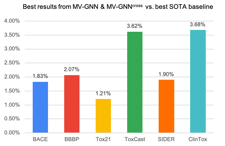
(a) Classification tasks.

(b) Regression tasks.

Figure 9: Improvement visualization between best $\mathsf{MV}$-$\mathsf{GNN}$ models with the best SOTA model on classification tasks (Figure 9(a)) and regression tasks (Figure 9(b)).

E.6 Additional Results of Regression Tasks

Table 7 reports the results of $\mathsf{MV}$-$\mathsf{GNN}$ and $\mathsf{MV}$-${\mathsf{GNN^{cross}}}$ on regression tasks over 5 benchmark datasets and 7 baseline models. As we can see, $\mathsf{MV}$-$\mathsf{GNN}$ models achieve the best performance on regression tasks too. Recent graph studies on molecules generally focus on certain areas which lack universality. For example, $\mathsf{SchNet}$ and $\mathsf{MGCN}$ perform good on quantum mechanics datasets (QM7 and QM8) since they utilizes the distances between atoms using the 3D coordinate information, but cannot capture sufficient molecule-level information to generate accurate molecular representations. On the other hand, our $\mathsf{MV}$-$\mathsf{GNN}$ models consistently achieve remarkable performance over all datasets. Specifically, our methods relatively improve 28.7% over other models on the FreeSolv dataset, yet again, reveals the superiority and robustness of the multi-view architecture. The results of $\mathsf{Concat+Mean}$ and $\mathsf{Concat+Attn}$ on regression datasets also prove the effectiveness of $\mathsf{MV}$-$\mathsf{GNN}$.

Figure 9(b) illustrates the relative improvement from our model with other SOTAs, according to Table 7. As shown in Figure 9(b), $\mathsf{MV}$-$\mathsf{GNN}$ models achieve average 16.6% improvement on the five regression benchmark datasets.

Table 7: Performance comparison on regression tasks based on scaffold split (smaller is better). Best score is marked as bold, and the best baseline is marked in gray background. Green cells indicate the results of our methods.

Method	QM7	QM8	ESOL	Lipo	FreeSolv
$\mathsf{GraphConv}$	118.875 ±20.219	0.021 ±0.001	1.068 ±0.050	0.712 ±0.049	2.900 ±0.135
$\mathsf{Weave}$	94.688 ±2.705	0.022 ±0.001	1.158 ±0.055	0.813 ±0.042	2.398 ±0.250
$\mathsf{SchNet}$	74.204±4.983	0.020±0.002	1.045±0.064	0.909±0.098	3.215±0.755
$\mathsf{MGCN}$	77.623±4.734	0.022±0.002	1.266±0.147	1.113±0.041	3.349±0.097
$\mathsf{N}$-$\mathsf{Gram}$	125.630±1.480	0.032±0.003	1.100±0.160	0.876±0.033	2.512±0.190
$\mathsf{MPNN}$	112.960 ±17.211	0.015 ±0.002	1.167 ±0.430	0.672 ±0.051	2.185 ±0.952
$\mathsf{DMPNN}$	105.775 ±13.202	0.0143 ±0.0023	0.980 ±0.258	0.653 ±0.046	2.177 ±0.914
$\mathsf{Concat+Mean}$	72.532 $\pm$ 2.657	0.0129 $\pm$ 0.0005	0.806$\pm$0.040	0.610$\pm$0.024	2.003$\pm$0.317
$\mathsf{Concat+Attn}$	73.132$\pm$3.845	0.0128$\pm$0.0005	0.809$\pm$0.043	0.601$\pm$0.015	2.026 $\pm$ 0.227
$\mathsf{MV}$-$\mathsf{GNN}$	71.325 ±2.843	0.0127 ±0.0005	0.8049 ±0.036	0.599 ±0.016	1.840 ±0.194
$\mathsf{MV}$-${\mathsf{GNN^{cross}}}$	70.358 ±5.962	0.0124 ±0.001	0.779±0.026	0.553 ±0.013	1.552 ±0.123

References

- [1] Han Altae-Tran, Bharath Ramsundar, Aneesh S Pappu, and Vijay Pande. Low data drug discovery with one-shot learning. ACS central science, 3(4):283–293, 2017.
- [2] Guy W Bemis and Mark A Murcko. The properties of known drugs. 1. molecular frameworks. Journal of medicinal chemistry, 39(15):2887–2893, 1996.
- [3] Sanjivanjit K Bhal. Logp—making sense of the value. Advanced Chemistry Development, Toronto, ON, Canada, pages 1–4, 2007.
- [4] L. C. Blum and J.-L. Reymond. 970 million druglike small molecules for virtual screening in the chemical universe database GDB-13. J. Am. Chem. Soc., 131:8732, 2009.
- [5] Antoine Bordes, Xavier Glorot, Jason Weston, and Yoshua Bengio. Joint learning of words and meaning representations for open-text semantic parsing. In Artificial Intelligence and Statistics, pages 127–135, 2012.
- [6] Leo Breiman. Random forests. Machine learning, 45(1):5–32, 2001.
- [7] Travers Ching, Daniel S Himmelstein, Brett K Beaulieu-Jones, Alexandr A Kalinin, Brian T Do, Gregory P Way, Enrico Ferrero, Paul-Michael Agapow, Michael Zietz, Michael M Hoffman, et al. Opportunities and obstacles for deep learning in biology and medicine. Journal of The Royal Society Interface, 15(141):20170387, 2018.
- [8] John S Delaney. Esol: estimating aqueous solubility directly from molecular structure. Journal of chemical information and computer sciences, 44(3):1000–1005, 2004.
- [9] David K Duvenaud, Dougal Maclaurin, Jorge Iparraguirre, Rafael Bombarell, Timothy Hirzel, Alán Aspuru-Guzik, and Ryan P Adams. Convolutional networks on graphs for learning molecular fingerprints. In NeurIPS, pages 2224–2232, 2015.
- [10] Alex Fout, Jonathon Byrd, Basir Shariat, and Asa Ben-Hur. Protein interface prediction using graph convolutional networks. In NeurIPS, pages 6530–6539, 2017.
- [11] Jerome Friedman, Trevor Hastie, Robert Tibshirani, et al. Additive logistic regression: a statistical view of boosting (with discussion and a rejoinder by the authors). The annals of statistics, 28(2):337–407, 2000.
- [12] Jerome H Friedman. Greedy function approximation: a gradient boosting machine. Annals of statistics, pages 1189–1232, 2001.
- [13] Anna Gaulton, Louisa J Bellis, A Patricia Bento, Jon Chambers, Mark Davies, Anne Hersey, Yvonne Light, Shaun McGlinchey, David Michalovich, Bissan Al-Lazikani, et al. Chembl: a large-scale bioactivity database for drug discovery. Nucleic acids research, 40(D1):D1100–D1107, 2011.
- [14] Kaitlyn M Gayvert, Neel S Madhukar, and Olivier Elemento. A data-driven approach to predicting successes and failures of clinical trials. Cell chemical biology, 23(10):1294–1301, 2016.
- [15] Justin Gilmer, Samuel S Schoenholz, Patrick F Riley, Oriol Vinyals, and George E Dahl. Neural message passing for quantum chemistry. In ICML, pages 1263–1272. JMLR. org, 2017.
- [16] Robert C Glen, Andreas Bender, Catrin H Arnby, Lars Carlsson, Scott Boyer, and James Smith. Circular fingerprints: flexible molecular descriptors with applications from physical chemistry to adme. IDrugs, 9(3):199, 2006.
- [17] Kelvin Guu, John Miller, and Percy Liang. Traversing knowledge graphs in vector space. arXiv preprint arXiv:1506.01094, 2015.
- [18] Will Hamilton, Payal Bajaj, Marinka Zitnik, Dan Jurafsky, and Jure Leskovec. Embedding logical queries on knowledge graphs. In Advances in Neural Information Processing Systems, pages 2026–2037, 2018.
- [19] Frank Harary and Robert Z. Norman. Some properties of line digraphs. Rendiconti del Circolo Matematico di Palermo, 9(2):161–168, May 1960.
- [20] Wenbing Huang, Tong Zhang, Yu Rong, and Junzhou Huang. Adaptive sampling towards fast graph representation learning. In NeurIPS, pages 4558–4567. 2018.
- [21] Stanisław Jastrzębski, Damian Leśniak, and Wojciech Marian Czarnecki. Learning to smile (s). arXiv preprint arXiv:1602.06289, 2016.
- [22] Steven Kearnes, Kevin McCloskey, Marc Berndl, Vijay Pande, and Patrick Riley. Molecular graph convolutions: moving beyond fingerprints. Journal of computer-aided molecular design, 30(8):595–608, 2016.
- [23] David G Kleinbaum, K Dietz, M Gail, Mitchel Klein, and Mitchell Klein. Logistic regression. Springer, 2002.
- [24] Johannes Klicpera, Janek Groß, and Stephan Günnemann. Directional message passing for molecular graphs. In International Conference on Learning Representations (ICLR), 2020.
- [25] Michael Kuhn, Ivica Letunic, Lars Juhl Jensen, and Peer Bork. The sider database of drugs and side effects. Nucleic acids research, 44(D1):D1075–D1079, 2015.
- [26] Greg Landrum et al. Rdkit: Open-source cheminformatics, 2006.
- [27] Jia Li, Yu Rong, Hong Cheng, Helen Meng, Wenbing Huang, and Junzhou Huang. Semi-supervised graph classification: A hierarchical graph perspective. In The World Wide Web Conference, pages 972–982. ACM, 2019.
- [28] Ruoyu Li, Sheng Wang, Feiyun Zhu, and Junzhou Huang. Adaptive graph convolutional neural networks. In AAAI, 2018.
- [29] Shengchao Liu, Mehmet F Demirel, and Yingyu Liang. N-gram graph: Simple unsupervised representation for graphs, with applications to molecules. In Advances in Neural Information Processing Systems, pages 8464–8476, 2019.
- [30] Chengqiang Lu, Qi Liu, Chao Wang, Zhenya Huang, Peize Lin, and Lixin He. Molecular property prediction: A multilevel quantum interactions modeling perspective. In Proceedings of the AAAI Conference on Artificial Intelligence, volume 33, pages 1052–1060, 2019.
- [31] Mingsong Mao, Jie Lu, Guangquan Zhang, and Jinlong Zhang. Multirelational social recommendations via multigraph ranking. IEEE transactions on cybernetics, 47(12):4049–4061, 2016.
- [32] Ines Filipa Martins, Ana L Teixeira, Luis Pinheiro, and Andre O Falcao. A bayesian approach to in silico blood-brain barrier penetration modeling. Journal of chemical information and modeling, 52(6):1686–1697, 2012.
- [33] David L Mobley and J Peter Guthrie. Freesolv: a database of experimental and calculated hydration free energies, with input files. Journal of computer-aided molecular design, 28(7):711–720, 2014.
- [34] Federico Monti, Michael Bronstein, and Xavier Bresson. Geometric matrix completion with recurrent multi-graph neural networks. In Advances in Neural Information Processing Systems, pages 3697–3707, 2017.
- [35] HL Morgan. The generation of a unique machine description for chemical structures-a technique developed at chemical abstracts service. J. Chemical Documentation, 5:107–113, 1965.
- [36] Greeshma Neglur, Robert L Grossman, and Bing Liu. Assigning unique keys to chemical compounds for data integration: Some interesting counter examples. In International Workshop on Data Integration in the Life Sciences, pages 145–157. Springer, 2005.
- [37] Steven M Paul, Daniel S Mytelka, Christopher T Dunwiddie, Charles C Persinger, Bernard H Munos, Stacy R Lindborg, and Aaron L Schacht. How to improve r&d productivity: the pharmaceutical industry’s grand challenge. Nature reviews Drug discovery, 9(3):203, 2010.
- [38] Douglas EV Pires, Tom L Blundell, and David B Ascher. pkcsm: predicting small-molecule pharmacokinetic and toxicity properties using graph-based signatures. Journal of medicinal chemistry, 58(9):4066–4072, 2015.
- [39] Kristina Preuer, Günter Klambauer, Friedrich Rippmann, Sepp Hochreiter, and Thomas Unterthiner. Interpretable deep learning in drug discovery. In Explainable AI: Interpreting, Explaining and Visualizing Deep Learning, pages 331–345. Springer, 2019.
- [40] Raghunathan Ramakrishnan, Mia Hartmann, Enrico Tapavicza, and O Anatole Von Lilienfeld. Electronic spectra from tddft and machine learning in chemical space. The Journal of chemical physics, 143(8):084111, 2015.
- [41] Ann M Richard, Richard S Judson, Keith A Houck, Christopher M Grulke, Patra Volarath, Inthirany Thillainadarajah, Chihae Yang, James Rathman, Matthew T Martin, John F Wambaugh, et al. Toxcast chemical landscape: paving the road to 21st century toxicology. Chemical research in toxicology, 29(8):1225–1251, 2016.
- [42] David Rogers and Mathew Hahn. Extended-connectivity fingerprints. Journal of chemical information and modeling, 50(5):742–754, 2010.
- [43] Yu Rong, Wenbing Huang, Tingyang Xu, and Junzhou Huang. Dropedge: Towards deep graph convolutional networks on node classification. In International Conference on Learning Representations, 2020.
- [44] Seongok Ryu, Jaechang Lim, Seung Hwan Hong, and Woo Youn Kim. Deeply learning molecular structure-property relationships using attention-and gate-augmented graph convolutional network. arXiv preprint arXiv:1805.10988, 2018.
- [45] J Saarikoski and M Viluksela. Influence of ph on the toxicity of substituted phenols to fish. Archives of environmental contamination and toxicology, 10(6):747–753, 1981.
- [46] Franco Scarselli, Marco Gori, Ah Chung Tsoi, Markus Hagenbuchner, and Gabriele Monfardini. The graph neural network model. IEEE Transactions on Neural Networks, 20(1):61–80, 2008.
- [47] Kristof Schütt, Pieter-Jan Kindermans, Huziel Enoc Sauceda Felix, Stefan Chmiela, Alexandre Tkatchenko, and Klaus-Robert Müller. Schnet: A continuous-filter convolutional neural network for modeling quantum interactions. In Advances in neural information processing systems, pages 991–1001, 2017.
- [48] Kristof T Schütt, Farhad Arbabzadah, Stefan Chmiela, Klaus R Müller, and Alexandre Tkatchenko. Quantum-chemical insights from deep tensor neural networks. Nature communications, 8:13890, 2017.
- [49] Chao Shang, Qinqing Liu, Ko-Shin Chen, Jiangwen Sun, Jin Lu, Jinfeng Yi, and Jinbo Bi. Edge attention-based multi-relational graph convolutional networks. arXiv preprint arXiv:1802.04944, 2018.
- [50] Govindan Subramanian, Bharath Ramsundar, Vijay Pande, and Rajiah Aldrin Denny. Computational modeling of -secretase 1 (bace-1) inhibitors using ligand based approaches. Journal of chemical information and modeling, 56(10):1936–1949, 2016.
- [51] Shiliang Sun. A survey of multi-view machine learning. Neural computing and applications, 23(7-8):2031–2038, 2013.
- [52] S Joshua Swamidass, Chloé-Agathe Azencott, Ting-Wan Lin, Hugo Gramajo, Shiou-Chuan Tsai, and Pierre Baldi. Influence relevance voting: an accurate and interpretable virtual high throughput screening method. Journal of chemical information and modeling, 49(4):756–766, 2009.
- [53] Ashish Vaswani, Noam Shazeer, Niki Parmar, Jakob Uszkoreit, Llion Jones, Aidan N Gomez, Lukasz Kaiser, and Illia Polosukhin. Attention is all you need. In Advances in neural information processing systems, pages 5998–6008, 2017.
- [54] Petar Veličković, Guillem Cucurull, Arantxa Casanova, Adriana Romero, Pietro Lio, and Yoshua Bengio. Graph attention networks. arXiv preprint arXiv:1710.10903, 2017.
- [55] Minjie Wang, Lingfan Yu, Da Zheng, Quan Gan, Yu Gai, Zihao Ye, Mufei Li, Jinjing Zhou, Qi Huang, Chao Ma, Ziyue Huang, Qipeng Guo, Hao Zhang, Haibin Lin, Junbo Zhao, Jinyang Li, Alexander J Smola, and Zheng Zhang. Deep graph library: Towards efficient and scalable deep learning on graphs. ICLR Workshop on Representation Learning on Graphs and Manifolds, 2019.
- [56] David Weininger, Arthur Weininger, and Joseph L Weininger. Smiles. 2. algorithm for generation of unique smiles notation. Journal of chemical information and computer sciences, 29(2):97–101, 1989.
- [57] Boris Weisfeiler and Andrei A Lehman. A reduction of a graph to a canonical form and an algebra arising during this reduction. Nauchno-Technicheskaya Informatsia, 2(9):12–16, 1968.
- [58] Zhenqin Wu, Bharath Ramsundar, Evan N Feinberg, Joseph Gomes, Caleb Geniesse, Aneesh S Pappu, Karl Leswing, and Vijay Pande. Moleculenet: a benchmark for molecular machine learning. Chemical Science, 9(2):513–530, 2018.
- [59] Zhaoping Xiong, Dingyan Wang, Xiaohong Liu, Feisheng Zhong, Xiaozhe Wan, Xutong Li, Zhaojun Li, Xiaomin Luo, Kaixian Chen, Hualiang Jiang, et al. Pushing the boundaries of molecular representation for drug discovery with the graph attention mechanism. Journal of medicinal chemistry, 2019.
- [60] Keyulu Xu, Weihua Hu, Jure Leskovec, and Stefanie Jegelka. How powerful are graph neural networks? arXiv preprint arXiv:1810.00826, 2018.
- [61] Zheng Xu, Sheng Wang, Feiyun Zhu, and Junzhou Huang. Seq2seq fingerprint: An unsupervised deep molecular embedding for drug discovery. In BCB, 2017.
- [62] Kevin Yang, Kyle Swanson, Wengong Jin, Connor Coley, Philipp Eiden, Hua Gao, Angel Guzman-Perez, Timothy Hopper, Brian Kelley, Miriam Mathea, et al. Analyzing learned molecular representations for property prediction. Journal of chemical information and modeling, 59(8):3370–3388, 2019.