Lorentzian Toda field theories

Abstract:

We propose several different types of construction principles for new classes of Toda field theories based on root systems defined on Lorentzian lattices. In analogy to conformal and affine Toda theories based on root systems of semi-simple Lie algebras, also their Lorentzian extensions come about in conformal and massive variants. We carry out the Painlevé integrability test for the proposed theories, finding in general only one integer valued resonance corresponding to the energy-momentum tensor. Thus most of the Lorentzian Toda field theories are not integrable, as the remaining resonances, that grade the spins of the W-algebras in the semisimple cases, are either non integer or complex valued. We analyse in detail the classical mass spectra of several massive variants. Lorentzian Toda field theories may be viewed as perturbed versions of integrable theories equipped with an algebraic framework.

1 Introduction

Toda theories are one of the best studied and understood classical and quantum integrable systems. The integrability of their classical discrete lattice versions [1] is known for a long time and has been established by the construction of explicit Lax pairs [2] as well as the application of the Painlevé integrability test [3]. Their continuous field theoretical versions are scalar field theories defined by Lagrangians of the general form

$$\mathcal{L}_{{}_{\mathbf{g}_{-n}}}=\frac{1}{2}\partial_{\mu}\phi\cdot\partial^{\mu}\phi-\frac{g}{\beta^{2}}\sum\limits_{i=-n}^{r}e^{\beta\alpha_{i}\cdot\phi},$$ (1)

with coupling constants $g,\beta\in\mathbb{R}$ or $\beta\in i\mathbb{R}$. The $r+n+1$ vectors $\alpha_{i}$ of dimension $\ell+2m$ are taken to be roots on a lattice associated to some Lie algebras and the scalar field $\phi(x,t)$ has in general $\ell+2m$ components, i.e. $\phi^{a}(x,t)$ with $a=1,\ldots,\ell+2m$. Folded versions may also been constructed in which some field components are identified in very specific ways, see e.g. [4].

Many versions of the Lagrangians in (1) have been well studied. For instance, for $\ell=r$, $m=0$, $n=-1$ with $\alpha_{i}$ taken to be the simple roots of a semisimple Lie algebra $\mathbf{g}$, the Lagrangians $\mathcal{L}_{{}_{\mathbf{g}_{1}}}$corresponds to the well known description of conformal Toda field theory, see e.g. [5, 6]. When $\ell=r$, $m=0$, $n=0$, with $\alpha_{0}$ taken to be the negative of the highest root, the Lagrangians $\mathcal{L}_{{}_{\mathbf{g}_{0}}}$corresponds to affine Toda field theory with $r$ massive scalar fields, see for instance e.g. [7, 8]. Similarly as for their discrete counterparts, the classical integrability of these continuous systems has been established by the explicit construction of Lax pairs or zero curvature expressions [9, 10, 11, 12]. Since the classical equations of motion are nonlinear integrable equations, they possess solutions of with very rich solitonic structures [13, 14, 15, 16, 17]. One of the most remarkable properties of these systems is the fact that the quantum scattering matrices for affine Toda field theories have been constructed to all orders in perturbation theory by using what is referred to as the bootstrap approach [18, 19, 20, 21, 7, 22, 23]. For theories based on simply laced Lie algebras this has been possible due to the fact that the classical mass ratios [8] are preserved to all orders in perturbation theory [18, 19, 20, 21, 24]. For non-simply laced theories the masses renormalize with different factors, but, nonetheless, closed exact expressions for the scattering matrices were still found [25, 26] by exploiting properties of q-deformed Coxeter elements. Once again the root space provides the general framework, where in this case the dual affine algebras correspond to the two classical limits of very weak or very strong coupling. While the Yang-Baxter equation is trivially satisfied by the scattering matrices describing theories with real coupling constants $\beta\in\mathbb{R}$, it possesses non-trivial solutions characterized by their quantum group symmetries when $\beta\in i\mathbb{R}$ is taken to be purely imaginary [27]. The S-matrices factorize into the so-called minimal and CDD factor, with the former describing the scattering in the Restricted Solid-on-Solid (RSOS)-models and the latter containing the coupling constant.

While all of the above theories are integrable and based on root systems that lead to a positive definite or semi-definite Cartan matrix, some attempts have been made to extend the theories in (1) and formulate them on root systems corresponding to hyperbolic Kac Moody algebras [28]. These algebras have been fully classified [29] and proven to be very useful in a string/M theory context [30], with $E_{10}$ being a popular example. However, it has turned that $E_{11}$, which is not a hyperbolic Kac Moody algebra [31], is even more useful. It belongs to the larger class of algebras that are Lorentzian [32, 33, 34]. A particular subclass of them studied in [33], is defined in terms of their connected Dynkin diagrams so that the deletion of at least one node leaves a possibly disconnected set of connected Dynkin diagrams each of which is of finite type, except for at most one affine type. In [34] an even larger class of $n$-extended Lorentzian Kac Moody algebras was introduced. Here the aim is to investigate the properties of Toda field theories described by the Lagrangians in (1) based on these Lorentzian type of root systems.

Since the algebras discussed come along with a classification scheme based on their root systems, the above results have proven very successfully that the physical properties of the theories based on them can be characterized very systematically. In has turned out that theories in the same subclass share the same general properties. These subclasses may be defined for instance by being simply laced or non-simply laced, semisimple or affine, having real or purely imaginary coupling constants, being hyperbolic, etc. It has turned out that Toda field theories based on root systems corresponding to hyperbolic Kac Moody algebras are not integrable as they do not pass the Painlevé test [28]. However, similarly as their integrable cousins, they, together with the theories of Lorentzian type discussed here, provide a systematic framework for the study of nonintegrable quantum field theories [35]. We take these two aspects as our main motivation to study Lorentzian Toda field theories.

To set up these new systems we need to specify not only the limits in the sum in (1), the dimension of the representation space of the roots and the choice of the highest root similarly as for the conformal and affine cases, but in addition we also have to re-defined the inner product in the kinetic term between the derivatives of the fields and in the potential term between the roots and the scalar field. These new inner products will place the theories onto Lorentzian lattice.

Our manuscript is structured as follows: In section 2 we introduce our definition and some key properties of the Lorentzian inner products. In addition, we introduce several matrices that are central for our analysis. In section 3 we employ these products to set up our Lorentzian Toda field theories. In section 4 we carry our the Painlevé integrability test for these theories. The test can be entirely reduced to an eigenvalue problem of what we refer to as the Painlevé matrix, that we analyse in section 5. In section 6 we discuss in detail the classical mass spectra of Lorentzian Toda field theories produced from different schemes. Our conclusions are stated in section 7.

2 Lorentzian products, the K, M, $\Lambda$, D and Painlevé matrices

The main difference between theories based on root systems for semisimple or affine algebras is the re-definition of the inner product between the derivatives of the scalar fields and between the roots and the scalar fields in kinetic and the potential term in (1), respectively. Following [33, 34], we define here the following Lorentzian inner products for two $\ell+2m$ dimensional vectors $x=(x_{1},\ldots,x_{\ell+2m})$ and $y=(y_{1},\ldots,y_{\ell+2m})$ as

$$x\cdot y:=\sum\limits_{\beta=1}^{\ell}x_{\beta}y_{\beta}-\sum\limits_{\beta=1}^{m}\left(x_{\ell+2\beta-1}y_{\ell+2\beta}+x_{\ell+2\beta}y_{\ell+2\beta-1}\right).$$ (2)

We extend the definition of this product to matrix multiplication in a natural way. For a $N\times\left(\ell+2m\right)$-matrix $A$ and a $\left(\ell+2m\right)\times N$-matrix $B$, we define

$$\left(AB\right)_{ij}:=\sum\limits_{\beta=1}^{\ell}A_{i\beta}B_{\beta j}-\sum\limits_{\beta=1}^{m}\left[A_{i\left(\ell+2\beta-1\right)}B_{\left(\ell+2\beta\right)j}+A_{i\left(\ell+2\beta\right)}B_{\left(\ell+2\beta-1\right)j}\right],~{}\ i,j=1,\ldots,N.$$ (3)

In particular, taking now $N=r+n+1$ we define a $(r+n+1)\times\left(\ell+2m\right)$-matrix $M$ with rows comprised of $r+n+1$ root vectors $\alpha_{i}=$ $(\alpha_{i}^{1},\ldots,\alpha_{i}^{{}_{\ell+2m}})^{T}$ of dimension $\ell+2m$, i.e. $M_{i\beta}:=\alpha_{i}^{\beta}$. When $r+n+1\leq\ell+2m$ the matrix $M$ possess a right inverse, which is obtained by defining a $\left(\ell+2m\right)\times(r+n+1)$-matrix $\Lambda$ with columns comprised of $r+n+1$ fundamental weight vectors $\lambda_{i}=$ $(\lambda_{i}^{1},\ldots,\lambda_{i}^{{}_{\ell+2m}})$ of dimension $\ell+2m$, i.e. $\Lambda_{\beta i}:=\lambda_{i}^{\beta}$. Hence with

$$M_{i\beta}:=\alpha_{i}^{\beta},\qquad\Lambda_{\beta i}:=\lambda_{i}^{\beta},~{}~{}\ \ \ ~{}i=1,\ldots,r+n+1\text{; }\beta=1,\ldots,\ell,\text{ }$$ (4)

we obtain

$$\left(M\Lambda\right)_{ij}=\alpha_{i}\cdot\lambda_{j}=\delta_{ij}=\lambda_{i}\cdot\alpha_{j}=\left(\Lambda^{T}M^{T}\right)_{ij}.$$ (5)

Moreover, we may employ $M$, $M^{T}$ and $\Lambda$, $\Lambda^{T}$ to factorize the symmetric Cartan matrix $K$ and their inverse $K^{-1}$, respectively, as

$$\left(MM^{T}\right)_{ij}=\alpha_{i}\cdot\alpha_{j}=K_{ij},\quad\text{and\quad}\left(\Lambda\Lambda^{T}\right)_{ij}=\lambda_{i}\cdot\lambda_{j}=K_{ij}^{-1}.$$ (6)

In general the Cartan matrix is defined as $2\alpha_{i}\cdot\alpha_{j}/\alpha_{j}^{2}$, which only in the symmetric case may be reduced to $\alpha_{i}\cdot\alpha_{j}$ when taking the length of the roots to be $2$. Since below we shall also encounter roots of length $0$, we adopt here the symmetric definition. When summing over one index of the inverse symmetric Cartan matrix we obtain some constants

$$D_{k}:=\sum_{j=-n}^{r}K_{kj}^{-1}=\rho\cdot\lambda_{k},~{}~{}~{}\ \ \ k=-n,\ldots,-1,0,1,\ldots,r,$$ (7)

that encode information about the existence of $SO(1,2)$ and $SO(3)$ principal subalgebras and the decomposition of the root lattices with their corresponding algebras [33, 34]. As stated in (7) the constants $D_{k}$ can also be computed directly from their Lorentzian inner products of weight vectors $\lambda_{k}$ with the Weyl vector $\rho$. Using these constants to define a diagonal matrix $D:=\mathop{\mathrm{d}iag}(D_{r},\ldots,D_{-n})$ we introduce a further matrix

$$P:=2DK,$$ (8)

referred to here as the Painlevé matrix. As we will see below the Painlevé integrability test can be reduced entirely to an eigenvalue problem for this matrix.

In what follows below we will take all inner products and matrix multiplications as specified in this subsection.

3 Perturbed $\mathcal{L}_{{}_{\mathbf{g}_{-1}}}$-Lorentzian Toda field theory

Let us now discuss some theories with the root system enlarged to a Lorentzian lattice. We start by illustrating the construction principle for the perturbation of some over extended algebra $\mathbf{g}_{-1}$.

To define these systems we need to enlarge the root space. Adopting the conventions from [33, 34], the root lattice $\Lambda_{\mathbf{g}}$ of the semisimple Lie algebra $\mathbf{g}$ is extended by a self-dual Lorentzian lattice $\Pi^{1,1}$ to

$$\Lambda_{\mathbf{g}_{-1}}=\Lambda_{\mathbf{g}}\oplus\Pi^{1,1}.$$ (9)

The root space $\Pi^{1,1}$ contains two null vectors $k$ and $\bar{k}$ with $k\cdot k=\bar{k}\cdot\bar{k}=0$, $k\cdot\bar{k}=1$ and two vectors $\pm\left(k+\bar{k}\right)$ of length $2$. The simple root system consists in this case of the $r$ simple roots $\alpha_{1},\ldots,\alpha_{r}~{}$of the semisimple Lie algebra $\mathbf{g}$, the modified affine root $\alpha_{0}=k-\sum\nolimits_{i=1}^{r}n_{i}\alpha_{i}$, with $n_{i}\in\mathbb{N}$ denoting the Kac labels, and the Lorentzian root $\alpha_{-1}=-\left(k+\bar{k}\right)$.

For the corresponding Lagrangians the construction is summarized as follows

$$\mathcal{L}_{{}_{\mathbf{g}_{1}}}\overset{\alpha_{0}}{\rightarrow}\mathcal{L}_{{}_{\mathbf{g}_{0}}}\overset{\alpha_{-1}}{\rightarrow}\mathcal{L}_{{}_{\mathbf{g}_{-1}}}\overset{\alpha_{-2}}{\rightarrow}\mathcal{L}_{{}_{\mathbf{\mathring{g}}_{-2}}}.$$ (10)

We have started here with the standard conformal Toda field theory $\mathcal{L}_{{}_{\mathbf{g}_{1}}}$ and added the modified root $\alpha_{0}$ to obtain the massive affine Toda field theory $\mathcal{L}_{{}_{\mathbf{g}_{0}}}$. Adding the root $\alpha_{-1}$ yields the scalar field theory described by the Lagrangian $\mathcal{L}_{{}_{\mathbf{g}_{-1}}}$, which turns out to be conformal and can be identified with a theory that is sometimes referred to as conformal affine Toda field theory [36, 37]. The corresponding algebra is an over extended algebra, of which for instance $(E_{8})_{-1}$ aka $E_{10}$ is of relevance in a string/M-theory context [30]. We discuss now this theory in some detail before we state how the root $\alpha_{-2}$ is constructed in order to obtain the massive $\mathcal{L}_{{}_{\mathbf{\mathring{g}}_{-2}}}$-theory.

The classical equations of motion for $\mathcal{L}_{{}_{\mathbf{g}_{-1}}}$, resulting from $\partial_{\mu}\left[\partial\mathcal{L}/\partial(\partial_{\mu}\phi^{a})\right]=\partial\mathcal{L}/\phi^{a}$, are

$$\square\phi^{a}+\frac{g}{\beta^{2}}\sum\limits_{i=-1}^{r}\alpha_{i}^{a}e^{\beta\alpha_{i}\cdot\phi}=0,\qquad a=1,\ldots,\ell+2.$$ (11)

We may view the potential in $\mathcal{L}_{{}_{\mathbf{g}_{-1}}}$as a perturbation of an affine Toda field theory with potential $\mathcal{V}_{{}_{\mathbf{g}_{0}}}$ so that $\mathcal{V}_{{}_{\mathbf{g}_{-1}}}=$ $\mathcal{V}_{{}_{\mathbf{g}_{0}}}+\delta\mathcal{V}_{{}_{\mathbf{g}_{0}}}$, where $\delta\mathcal{V}_{{}_{\mathbf{g}_{0}}}$ corresponds to the term in the sum related to $\alpha_{-1}$.

Since $\mathcal{V}_{{}_{\mathbf{g}_{0}}}$ possess a proper vacuum around which one may expand, it is clear that the additional term $\delta\mathcal{V}_{{}_{\mathbf{g}_{0}}}$ will spoil this property, unless it vanishes by itself for the value of the vacuum, and the right hand sides in (11) only vanish for $\alpha_{i}\cdot\phi\rightarrow-\infty$. An alternative way to verify whether a theory is conformally invariant or massive is to use the well-known property of the trace of the improved energy momentum tensor, that is zero or nonvanishing, respectively. For this purpose we first transform the equation of motion into a more convenient form by defining a new field $\Phi_{i}:=\alpha_{i}\cdot\phi-\beta^{-1}\ln(2\alpha_{i}^{-2})$, such that the equation of motion (11) converts into

$$\square\Phi_{j}+\frac{g}{\beta^{2}}\sum\limits_{i=-1}^{r}K_{ji}e^{\beta\Phi_{j}}=0,$$ (12)

with $K_{ij}:=2\alpha_{i}\cdot\alpha_{j}/\alpha_{j}^{2}$ denoting the Cartan matrix, which we assume here to be symmetric, i.e. $\alpha_{j}^{2}=2$. Defining further the fields $\varphi_{i}$ through the relations $\Phi_{i}=\left(M\varphi\right)_{i}$, where the matrix $M$ defined in (4) factorizes the Cartan matrix as in (6), we obtain the following version of the equation of motion

$$\square\varphi_{\alpha}+\frac{g}{\beta^{2}}\sum\limits_{i=-1}^{r}\left(M^{T}\right)_{\alpha i}e^{\beta\left(M\varphi\right)_{i}}=0.$$ (13)

Following [5, 6], the trace of the improved energy tensor results to

$$\Theta_{~{}\mu}^{\mu}=\sum\limits_{i=-1}^{r}\left(\frac{2g}{\beta^{2}}e^{\beta\left(M\varphi\right)_{i}}+\gamma_{i}\square\varphi_{i}\right).$$ (14)

Thus for $\gamma_{i}=2\beta^{-1}\sum_{k}M_{ik}^{-1}$ we obtain the equation of motion for each term in the sum and the trace of the improved energy tensor vanishes. In turn, this means when the matrix $M$ is not invertible the model is not conformally invariant and hence massive.

While $\mathcal{L}_{{}_{\mathbf{g}_{-1}}}$ is a massless conformally invariant theory, which might be studied in its own right, here we are interested in the question of whether it is possible to construct a massive field theory and therefore add consistently a perturbing term to $\mathcal{V}_{{}_{\mathbf{g}_{-1}}}$

$$\mathcal{V}_{{}_{\mathbf{\mathring{g}}_{-2}}}(\phi):=\mathcal{V}_{{}_{\mathbf{g}_{-1}}}(\phi)+\delta\mathcal{V}_{{}_{\mathbf{g}_{-1}}}(\phi)=\mathcal{V}_{{}_{\mathbf{g}_{-1}}}(\phi)+\varepsilon\frac{g}{\beta^{2}}e^{\beta\alpha_{-2}\cdot\phi}.$$ (15)

The vacuum $\phi^{(0)}$ for the new potential $\mathcal{V}_{{}_{\mathbf{\mathring{g}}_{-2}}}$ computed from the equations $\left.\partial\mathcal{V}_{{}_{\mathbf{\mathring{g}}_{-2}}}/\partial\phi^{a}\right|_{\phi^{(0)}}=0$, $a=1,\ldots,r+2$, leads to the constraint

$$\sum\limits_{i=-1}^{r}\alpha_{i}e^{\beta\alpha_{i}\cdot\phi^{(0)}}=-\varepsilon\alpha_{-2}e^{\beta\alpha_{-2}\cdot\phi^{(0)}}.$$ (16)

Multiplying with the fundamental weights $\lambda_{j}$ and using the orthogonality relation $\alpha_{i}\cdot\lambda_{j}=\delta_{ij}$ yields the relations

$$e^{\beta\alpha_{i}\cdot\phi^{(0)}}=-\varepsilon\lambda_{i}\cdot\alpha_{-2}e^{\beta\alpha_{-2}\cdot\phi^{(0)}},\qquad i=-1,0,1,\ldots,r.$$ (17)

Expanding now the potential $\mathcal{V}_{{}_{\mathbf{\mathring{g}}_{-2}}}(\phi)$ around the vacuum we obtain with (17)

$$\mathcal{V}_{{}_{\mathbf{\mathring{g}}_{-2}}}(\phi^{(0)}+\tilde{\phi})=\varepsilon\frac{g}{\beta^{2}}e^{\beta\alpha_{-2}\cdot\phi^{(0)}}\left[e^{\beta\alpha_{-2}\cdot\tilde{\phi}}-\sum\limits_{i=-1}^{r}\lambda_{i}\cdot\alpha_{-2}e^{\beta\alpha_{i}\cdot\tilde{\phi}}\right]=\frac{m^{2}}{\beta^{2}}\sum\limits_{i=-2}^{r}\hat{n}_{i}e^{\beta\alpha_{i}\cdot\tilde{\phi}},$$ (18)

where $m^{2}=\varepsilon ge^{\beta\alpha_{-2}\cdot\phi^{(0)}}$, $\hat{n}_{-2}=1$ and $\hat{n}_{i}=-\lambda_{i}\cdot\alpha_{-2}$.

We now make the choice $\alpha_{-2}=\bar{k}$, so that with the realizations of the fundamental weights for $\mathbf{g}_{-1}$ as [33, 34]

$$\lambda_{i}=\lambda_{i}^{f}+n_{i}\lambda_{0}^{o},~{}~{}\ \lambda_{0}=\bar{k}-k,\quad\lambda_{-1}=-k,~{}~{}~{}\text{with }i=1,\ldots,r,$$ (19)

and $\lambda_{i}$ denoting the fundamental weights of $\mathbf{g}$, we compute $\hat{n}_{-1}=1$, $\hat{n}_{0}=1$ and $\hat{n}_{i}=n_{i}$. Notice that $\mathbf{\mathring{g}}_{-2}$ is not a proper over extended algebra as defined in [34], hence the notation $\mathbf{\mathring{g}}_{-2}$ instead of $\mathbf{g}_{-2}$. We have $\alpha_{-2}\in$ $\Lambda_{\mathbf{g}}\oplus\Pi^{1,1}$ connecting in an almost identical way as the root $k-\left(\ell+\bar{\ell}\right)$ to all the other simple roots with $\alpha_{-2}\cdot\alpha_{-1}=-1$, $\alpha_{-2}\cdot\alpha_{i}=0$, $i=1,\ldots,r$. However, this root also connects to the affine root $\alpha_{-2}\cdot\alpha_{0}=1$, has length zero, i.e. $\alpha_{-2}^{2}=0\neq 2$, and is defined in a smaller representation space than the standard $\alpha_{-2}$-root. Hence $\Lambda_{\mathbf{\mathring{g}}_{-2}}$ can not be viewed as a lattice related to a Kac-Moody algebra and we refer to it therefore as a root lattice to an almost over extended algebra.

Expanding now (18) around zero we obtain a constant term in the potential of the form $m^{2}/\beta^{2}(\hat{n}_{-2}+\hat{n}_{-1}+\hat{n}_{0}+\sum\nolimits_{i=1}^{r}n_{i}$ $)=m^{2}/\beta^{2}(2+h)$ with $h$ denoting the Coxeter number of $\mathbf{g}$. Crucially, our choice for $\alpha_{-2}$ also has the desired property that the linear term in the expansion vanishes, because $\sum\nolimits_{i=-2}^{r}\hat{n}_{i}\alpha_{i}=0$. Labeling rows and columns as $(\tilde{\phi}_{1},\ldots,\tilde{\phi}_{r+2})$ the square mass matrix is obtained as

$$M^{2}=m^{2}\sum\limits_{i=-2}^{r}\hat{n}_{i}\left(\begin{array}[]{ccccc}\alpha_{i}^{1}\alpha_{i}^{1}&\ldots&\alpha_{i}^{1}\alpha_{i}^{r}&-\alpha_{i}^{1}\alpha_{i}^{r+2}&-\alpha_{i}^{1}\alpha_{i}^{r+1}\\ \vdots&\ddots&\vdots&\vdots&\vdots\\ \alpha_{i}^{1}\alpha_{i}^{r}&\ldots&\alpha_{i}^{r}\alpha_{i}^{r}&-\alpha_{i}^{r}\alpha_{i}^{r+2}&-\alpha_{i}^{r}\alpha_{i}^{r+1}\\ -\alpha_{i}^{1}\alpha_{i}^{r+2}&\ldots&-\alpha_{i}^{r}\alpha_{i}^{r+2}&\alpha_{i}^{r+2}\alpha_{i}^{r+2}&\alpha_{i}^{r+1}\alpha_{i}^{r+2}\\ -\alpha_{i}^{1}\alpha_{i}^{r+1}&\ldots&-\alpha_{i}^{r}\alpha_{i}^{r+1}&\alpha_{i}^{r+1}\alpha_{i}^{r+2}&\alpha_{i}^{r+1}\alpha_{i}^{r+1}\end{array}\right).$$ (20)

The classical mass spectra resulting from (20) are only physically meaningful when the eigenvalues of $M^{2}$ are real and positive. Before we will discuss concrete examples below, we first establish whether these type of theories are integrable by performing the Painlevé integrability test.

4 Painlevé integrability test

We now largely follow the line of reasoning in [3, 28] and generalize the Painlevé test [38, 39, 40, 41, 42] in order to establish whether variations of the $\mathcal{L}_{{}_{\mathbf{g}_{-n}}}$ Lorentzian Toda theories and perturbations thereof are integrable. First we transform the equation of motion in version (13) into light-cone coordinates so that $\square=\partial_{-}\partial_{+}$. For the sake of brevity, we denote $\partial_{-}$ by an overdot and $\partial_{+}$ by an overdash, e.g. $\partial_{-}\varphi=:\dot{\varphi}$ and $\partial_{+}\varphi=:\acute{\varphi}$. For further convenience we set $g=\beta=1$. We start by separating the second order equation of motion into two two first order equations, which can be achieved by introduce two quantities, akin but not equal to canonical variables, as

$$P_{\alpha}=\dot{\varphi_{\alpha}},\qquad Q_{i}=e^{\left(M\varphi\right)_{i}},~{}~{}\ \ \ \ \ \alpha=1,\ldots,\ell+2m\text{,}i=1,\ldots,r+n+1.$$ (21)

Differentiating these quantities with respect to each light-cone coordinate we obtain

$$\acute{P}_{\alpha}=\square\varphi_{\alpha}=-\sum\limits_{i=-n}^{r}\left(M^{T}\right)_{\alpha i}Q_{i},~{}~{}~{}~{}~{}~{}~{}\dot{Q}_{i}=Q_{i}\left(MP\right)_{i}.$$ (22)

We now Painlevé expand $P_{\alpha}$ and $Q_{i}$, making the standard assumption that both quantities possess movable critical singularities in some field $\phi(x_{-},x_{+})\rightarrow 0$, whose leading order is determined by some positive integers $n_{p},n_{q}>0$

$$Q_{i}=\sum_{k=0}^{\infty}a_{i}^{(k)}\phi^{k-n_{q}},\hskip 11.38109pt~{}~{}~{}P_{\alpha}=\sum_{k=0}^{\infty}b_{\alpha}^{(k)}\phi^{k-n_{p}}.$$ (23)

Differentiating the expansions we obtain

$$\dot{Q}_{i}=\sum_{k=0}^{\infty}(k-n_{q})a_{i}^{(k)}\phi^{k-n_{q}-1}\dot{\phi}\hskip 2.84526pt,~{}~{}~{}~{}~{}\ \acute{P}_{\alpha}=\sum_{k=0}^{\infty}(k-n_{p})b_{\alpha}^{(k)}\phi^{k-n_{p}-1}\acute{\phi}.$$ (24)

Substituting next the expansions (23) and (24) into (22) and balancing the powers we obtain

$$(k-n_{p})\acute{\phi}b_{\alpha}^{(k)} = -\sum\limits_{i=-n}^{r}\left(M^{T}\right)_{\alpha i}a_{i}^{(k)},$$ (25)

$$(k-n_{q})\dot{\phi}a_{i}^{(k)} = \sum_{m=0}^{k}a_{i}^{(k-m)}\left(Mb^{(m)}\right)_{i},$$ (26)

with $n_{q}=n_{p}+1$. At this point we have to distinguish between two cases i) when the Cartan matrix is invertible and ii) when it is not.

4.1 Invertible Cartan matrix

For $k=0$ we can solve the equations (25) and (26) for the leading order coefficient functions when the Cartan matrix is invertible

$$a_{i}^{(0)}=-n_{p}n_{q}\dot{\phi}\acute{\phi}D_{i},~{}~{}\ ~{}~{}b_{\alpha}^{(0)}=-n_{q}\dot{\phi}\sum\limits_{i=-n}^{r}\left(M^{T}\right)_{\alpha i}D_{i},$$ (27)

where the $D_{i}$ are the constants as defined in (7).

Next we extract in (26) the terms in the sum for $m=0$ and $m=k$. Using also $\left(Mb^{(0)}\right)_{i}=-n_{q}\dot{\phi}$, we re-write (25) and (26) as

$$k\dot{\phi}a_{i}^{(k)}+n_{p}n_{q}\dot{\phi}\acute{\phi}D_{i}\left(Mb^{(k)}\right)_{i} = \sum_{m=1}^{k-1}a_{i}^{(k-m)}\left(Mb^{(m)}\right)_{i},$$ (28)

$$\sum\limits_{i=-n}^{r}\left(M^{T}\right)_{\alpha i}a_{i}^{(k)}+(k-n_{p})\acute{\phi}b_{\alpha}^{(k)} = 0.$$ (29)

These equations, (28) and (29), can be converted into matrix form

$$T^{(k)}X^{(k)}=Y^{(k)},$$ (30)

when defining the $N+M=(r+n+1)+(\ell+2m)$ dimensional column vectors

$$X^{(k)} = (a_{1}^{(k)},\cdots,a_{M}^{(k)},b_{1}^{(k)},\cdots,b_{N}^{(k)})^{T},$$ (31)

$$Y^{(k)} = \sum_{m=1}^{k-1}(a_{1}^{(k-m)}\left(Mb^{(m)}\right)_{1},\cdots,a_{M}^{(k-m)}\left(Mb^{(m)}\right)_{M},0,\cdots,0)^{T},$$ (32)

together with the $(M+N)\times(M+N)$-matrix

$$T^{(k)}=\left(\begin{array}[]{ll}A_{M\times M}^{(k)}&B_{M\times N}^{(k)}\\ C_{N\times M}^{(k)}&E_{N\times N}^{(k)}\end{array}\right).$$ (33)

The block matrices in $T$ have entries

$$A_{ij}^{(k)}=k\dot{\phi}\delta_{ij},\quad B_{i\alpha}^{(k)}=n_{p}n_{q}\dot{\phi}\acute{\phi}D_{i}M_{i\alpha},\quad C_{\alpha i}^{(k)}=\left(M^{T}\right)_{\alpha i},\quad E_{\alpha\beta}^{(k)}=(k-n_{p})\acute{\phi}\delta_{\alpha\beta}.$$ (34)

Equation (30) is the central equation for the Painlevé integrability test. It is a recursive equation that may in principle be solved iteratively at each level $k$ for the coefficient functions contained in $X^{(k)}$ as long as the matrix $T^{(k)}$ is invertible. Whenever this is not the case one is introducing a free parameter, a resonance in Painlevé integrability test parlance, into the set of equations. When there are enough resonances in the system as boundary conditions or integration constants, the system is passing the test and is said to be integrable.

Let us therefore compute the determinant of $T^{(k)}$. Using the identity

$$\det\left(\begin{array}[]{ll}A&B\\ C&E\end{array}\right)=\det\left(\begin{array}[]{ll}A&B\\ C&E\end{array}\right)\det\left(\begin{array}[]{cc}I&0\\ -E^{-1}C&I\end{array}\right)=\det(A-BE^{-1}C)\det(E),$$ (35)

we obtain

$$\det T^{(k)}=(k-n_{p})^{r+n}\acute{\phi}^{r+n+1}\dot{\phi}\det\left[k(k-n_{p})I-n_{p}(n_{p}+1)DK\right].$$ (36)

Apart from the pre-factor, for $n=n_{p}=1$ this reduces to the expression previously obtained in [28] for the hyperbolic Kac-Moody algebras. Taking now $n_{p}=1$, the matrix in the determinant becomes the Painlevé matrix and the last factor in (36) can be read as the characteristic equation for the matrix $P=2DK$ with eigenvalues $k(k-1)$. Thus we have found that also for the $\mathcal{L}_{{}_{\mathbf{g}_{-n}}}$ Lorentzian Toda theories the integrability test can be reduced to an eigenvalue problem for $P$. Nicolai and Olive noticed in [43] that this matrix also emerges from the adjoint action of the $SO(1,2)$ Casimir operator on the Cartan subalgebra and that in fact the eigenvalues are identical to the Casimir eigenvalues. In this generalised case a principal $SO(1,2)$-subalgebra does not always exist, as explicitly argued in [34] for many cases, so that it needs to be replaced in part by a principal $SO(3)$-subalgebra.

4.2 Non-invertible Cartan matrix

When the Cartan matrix is not invertible we can not derive (27) from the equations (25) and (26). As a specific theory that involves a non-invertible Cartan matrix let us know consider the $\mathcal{L}_{{}_{\mathbf{g}_{0}}}$-theory, corresponding to affine Toda theory. Of course in this case we know that the theory is integrable since exact Lax pairs have been constructed for the classical theory [12] and in the quantum case the S-matrix factorizes into two-particle S-matrices as a consequence of the integrability [7]. However, let us see how the Painlevé test can be implemented, since the same line of argumentation can then also be applied to some extended theories we consider below. Using the fact that $K_{ij}=\tilde{K}_{ij}$ for $i,j=1,\ldots,r$ with $\tilde{K}$ denoting the invertible Cartan matrix of $\mathbf{g}$, we can split off the last row and the last column from $K$. Then it is easily seen that (27) is replaced by

$$a_{i}^{(0)}=-n_{p}n_{q}\dot{\phi}\acute{\phi}\tilde{D}_{i}+n_{i}a_{0}^{(0)},~{}~{}\ ~{}~{}b_{\alpha}^{(0)}=-n_{q}\dot{\phi}\sum\limits_{i=1}^{r}\left(M^{T}\right)_{\alpha i}\tilde{D}_{i},$$ (37)

where $\tilde{D}_{i}:=\sum\nolimits_{j=1}^{r}\tilde{K}_{ij}^{-1}$ and the $n_{i}$ denote the Kac labels as defined after (9). Following now the same steps as in the previous subsection we derive the matrix $T$ with block matrices

$$A_{ij}^{(k)}=k\dot{\phi}\delta_{ij},\quad B_{i\alpha}^{(k)}=n_{p}n_{q}\dot{\phi}\acute{\phi}D_{i}M_{i\alpha}-n_{i}M_{i\alpha}a_{0}^{(0)},\quad C_{\alpha i}^{(k)}=\left(M^{T}\right)_{\alpha i},\quad E_{\alpha\beta}^{(k)}=(k-n_{p})\acute{\phi}\delta_{\alpha\beta},$$ (38)

where we defined $D_{0}:=0$. Taking now $a_{0}^{(0)}=0$, we notice that the only non-vanishing entry in the $0$-row of $T^{(k)}$ is $T_{00}^{(k)}=A_{00}^{(k)}=k\dot{\phi}$. We can then expand $\det T^{(k)}$ with respect to the first row and derive

$$\det T^{(k)}=k(k-n_{p})^{r+1}\acute{\phi}^{r+2}\dot{\phi}^{2}\det\left[k(k-n_{p})I_{r\times r}-n_{p}(n_{p}+1)\tilde{D}\tilde{K}\right],$$ (39)

with $\tilde{D}$, $\tilde{K}$ belonging to $\mathbf{g}$. Thus we have reduced the Painlevé test for the $\mathcal{L}_{{}_{\mathbf{g}_{0}}}$-theory to an eigenvalue problem for the matrix $n_{p}(n_{p}+1)\tilde{D}\tilde{K}$ associated to $\mathbf{g}$.

Thus we conclude that the integrability properties of the $\mathcal{L}_{{}_{\mathbf{g}}}$-theory are inherited by the $\mathcal{L}_{{}_{\mathbf{g}_{0}}}$-theory, that is when $\mathcal{L}_{{}_{\mathbf{g}}}$ is (non)integrable so is $\mathcal{L}_{{}_{\mathbf{g}_{0}}}$.

For simplicity we derived here the eigenvalue equation (36) for symmetric Cartan matrices. We may repeat the same line of argumentation by replacing in $M^{T}$ roots by coroots, $\alpha_{i}\rightarrow\hat{\alpha}_{i}=2\alpha_{i}/\alpha_{i}^{2}$ when $\alpha_{i}^{2}\neq 0$. Then it is easily seen that (36) generalizes to the nonsymmetric case for which the Cartan matrix is defined as $K_{ij}=2\alpha_{i}\cdot\alpha_{j}/\alpha_{j}^{2}$ when $\alpha_{j}^{2}\neq 0$ and remains $K_{ij}=\alpha_{i}\cdot\alpha_{j}$ when $\alpha_{j}^{2}=0$.

5 The characteristic equation of the Painlevé matrix

We will keep now $n_{p}=1$ and analyse the characteristic equation for the Painlevé matrix $P$ as defined in (8)

$$\det\left[k(k-1)I-P\right]=0,$$ (40)

in some more detail. As argued in the previous subsection, for any version of the Lorentzian Toda field theories to be integrable the eigenvalues of the Painlevé matrix must be integer valued and factorize as $k(k-1)$ with $k\in\mathbb{N}$. In particular, this means when the eigenvalues are negative the theory is not integrable. These cases can be identified easily. We need to argue differently depending on whether the matrix $D$ is positive or negative definite, semi-definite of indefinite:

Denoting by $\mathop{\mathrm{i}nd}A=e_{p}-e_{n}$ the index of the matrix $A$, defined as the difference between the positive and negative eigenvalues of $A$, $e_{p}$ and $e_{n}$, respectively, we have the relation

$$\mathop{\mathrm{i}nd}(\pm 2DK)=\mathop{\mathrm{i}nd}(K),$$ (41)

where the $+$sign holds for $D$ positive definite and the $-$sign for $D$ negative definite.

To prove this relation we first note that the matrix $\sqrt{\pm D}K\sqrt{\pm D}$ has the same eigenvalues as $\pm DK$. Here $\sqrt{\pm D}$ is the positive square root with the sign depending on whether $D$ is positive or negative definite. Next we invoke Sylvester’s theorem, see e.g. Theorem 12.3 in [44], which states that two symmetric square matrices $A$ and $B$ that are congruent to each other, i.e. $A=QBQ^{T}$ for some nonsingular matrix $Q$, have the same index. Applied to the above this means that $\mathop{\mathrm{i}nd}(\sqrt{\pm D}K\sqrt{\pm D})=\mathop{\mathrm{i}nd}(K)$, since $\sqrt{\pm D}^{T}=\sqrt{\pm D}$. Therefore with $\mathop{\mathrm{i}nd}(\sqrt{\pm D}K\sqrt{\pm D})=\mathop{\mathrm{i}nd}(\pm DK)$ we obtain (41).

When $D$ is semi-definite we can define a reduced $D$-matrix as $\hat{D}$ by setting the positive or negative entries to zero and use a reduced version of (41) as $\mathop{\mathrm{i}nd}(\pm 2\hat{D}K)=\mathop{\mathrm{i}nd}(K)$.

Since a necessary condition for passing the Painlevé test is that all eigenvalues of $2DK$ are positive, i.e. $\mathop{\mathrm{i}nd}(2DK)=\ell$ with $\ell$ denoting the rank of $K$, the relation (41) implies that $\mathop{\mathrm{i}nd}(\pm K)=\ell\,$. This means only Lorentzian Toda field theories based on positive or negative definite Cartan matrix can pass the Painlevé test. In turn this means that those theories build from non-definite Cartan matrices can not be integrable.

6 Constructions of Lorentzian Toda field theory

We will now construct various types of Toda field theories based on different versions of root systems corresponding to Lorentzian Kac-Moody algebras and their extensions. We will encounter conformally invariant and massive models.

6.1 $\mathcal{L}_{{}_{\mathbf{\mathring{g}}_{-n}}}$-extended Lorentzian Toda field theory

This first type of theories is a series constituting an infinite extension of the perturbed $\mathcal{L}_{{}_{\mathbf{g}_{-1}}}$-theory introduced in section 3.1. The theories in this series come in two variants: The $\mathcal{L}_{{}_{\mathbf{\mathring{g}}_{-n}}}$-Lorentzian Toda field theories for odd $n$ are conformally invariant and those for which $n$ is even are massive. As a construction principle we extend the one previously used for the perturbation of the $\mathcal{L}_{{}_{\mathbf{g}_{-1}}}$-theory and build the roots as follows. For the massless $\mathcal{L}_{{}_{\mathbf{\mathring{g}}_{-(2n-1)}}}$-theories we have the $r+2n$ roots

$$\begin{array}[]{ll}\alpha_{i}\equiv\text{simple roots of }\mathbf{g}&\text{for }j=1,\ldots,r,\\ \alpha_{-(2i-2)}=k_{i}-\sum\nolimits_{j=-(2i-3)}^{r}n_{j}\alpha_{j}{}{}{}&\text{for }i=1,\ldots,n,\\ \alpha_{-(2i-1)}=-(k_{i}+\bar{k}_{i})&\text{for }i=1,\ldots,n.\end{array}$$ (42)

We notice that the roots $\alpha_{-(2i-2)}$ have length zero for $i=2,\ldots,n$, have a standard inner product equal to $-1$ with nearest neighbour roots on the Dynkin diagram and a more unusual inner product equal to $1$ for next to nearest neighbours. The roots $\alpha_{-(2i-1)}$ have length $2$ for $i=1,\ldots,n$. Thus we have the inner products

$$\alpha_{-(2i-2)}^{2}=0,\quad\alpha_{-(2j-1)}^{2}=2,\quad\alpha_{-k}\cdot\alpha_{-(k+1)}=-1,\quad\alpha_{-2l}\cdot\alpha_{-(2l+2)}=1,$$ (43)

for $i=2,\ldots,n$, $j=1,\ldots,n$, $k=1,\ldots,2n-2$ and $l=0,1,\ldots,n-2$. At each affine root $\alpha_{0}$ the Dynkin diagram is extended by the following segment:

We used here the standard conventions for drawing Dynkin diagrams related to semi-simple Lie algebras in which vertices with bullets indicate roots of length $2$ and single line links between two vertices correspond to inner products of $-1$ between the two corresponding roots. We increase the set of rules by indicating roots of length $0$ with an empty circles and inner products of $1$ by dotted links between two vertices correspond to the roots. Such type of zero length roots and inner products equal to $1$ are not entirely unusual and also occur in the context of Lie superalgebras and of their affine extensions [45].

The corresponding Cartan matrix is

$$K_{\mathbf{\mathring{g}}_{-(2n-1)}}=\left(\begin{array}[]{llllccc}&&&q_{1}&0&\cdots&0\\ &K_{\mathbf{g}}&&\vdots&\vdots&&\vdots\\ &&&q_{r}&0&\cdots&0\\ q_{1}&\cdots&q_{r}&2&\lx@intercol-1\hfil\lx@intercol&\lx@intercol 1\hfil\lx@intercol&\lx@intercol 0\hfil\lx@intercol\\ \lx@intercol\hfil 0\hfil\lx@intercol&\lx@intercol\hfil\cdots\hfil\lx@intercol&\lx@intercol\hfil 0\hfil\lx@intercol&-1&\lx@intercol\hfil\lx@intercol&\lx@intercol\hfil\lx@intercol&\lx@intercol\hfil\lx@intercol\\ \lx@intercol\hfil\vdots\hfil\lx@intercol&\lx@intercol\hfil\hfil\lx@intercol&\lx@intercol\hfil\vdots\hfil\lx@intercol&1&\lx@intercol\hfil\lx@intercol&\lx@intercol\hat{K}_{2n-1}\hfil\lx@intercol&\lx@intercol\hfil\lx@intercol\\ \lx@intercol\hfil 0\hfil\lx@intercol&\lx@intercol\hfil\cdots\hfil\lx@intercol&\lx@intercol\hfil 0\hfil\lx@intercol&0&\lx@intercol\hfil\lx@intercol&\lx@intercol\hfil\lx@intercol&\lx@intercol\hfil\lx@intercol\end{array}\right)$$ (44)

with $q_{s}:=\alpha_{0}\cdot\alpha_{s}$, $s=1,\ldots,r$, and $(2n-1)\times(2n-1)$ matrix $\hat{K}_{2n-1}$ with entries

$$\hat{K}_{2i-1,2i-1}=2,\quad\hat{K}_{2j,2j}=0,\quad\hat{K}_{k,k+1}=-1,\quad\hat{K}_{2l,2l+2}=1,$$ (45)

for $i=1,\ldots,n$, $j=1,\ldots,n-1$, $k=1,\ldots,2n-2$ and $l=1,\ldots,n-2$.

Taking the same roots and adding one root at the end of the Dynkin diagram as the negative highest root, designed to make the linear term in the potential vanish, we obtain the massive $\mathcal{\mathring{L}}_{{}_{\mathbf{g}_{-(2n)}}}$-theory based on $r+2n+1$ roots

$$\begin{array}[]{ll}\alpha_{i}\equiv\text{simple roots of }\mathbf{g}&\text{for }j=1,\ldots,r,\\ \alpha_{-(2i-2)}=k_{i}-\sum\nolimits_{j=-(2i-3)}^{r}n_{j}\alpha_{j}{}{}{}&\text{for }i=1,\ldots,n,\\ \alpha_{-(2i-1)}=-(k_{i}+\bar{k}_{i})&\text{for }i=1,\ldots,n,\\ \alpha_{-(2n)}=-\sum\nolimits_{j=-(2n-1)}^{r}n_{j}\alpha_{j}.&\end{array}$$ (46)

Now at each affine root $\alpha_{0}$ the Dynkin diagram is extended by the segment:

The corresponding Cartan matrix is

$$K_{\mathbf{\mathring{g}}_{-2n}}=\left(\begin{array}[]{ccccccc}&&&q_{1}&0&\cdots&0\\ &K_{\mathbf{g}}&&\vdots&\vdots&&\vdots\\ &&&q_{r}&0&\cdots&0\\ q_{1}&\cdots&q_{r}&2&-1&1&0\\ 0&\cdots&0&-1&&&\\ \vdots&&\vdots&1&&\hat{K}_{2n}&\\ 0&\cdots&0&0&&&\end{array}\right)$$ (47)

where the entries of the $(2n)\times(2n)$ matrix $\hat{K}_{2n}$ are defined as in (45) with $i=1,\ldots,n$, $j=1,\ldots,n$, $k=1,\ldots,2n-1$ and $l=1,\ldots,n-1$.

For the Toda field theories constructed from these root systems it follows from section 4 and 5 that the Painlevé integrability test is entirely reduced to an eigenvalue problem for the Painlevé matrix $P$, which must factor as $n(n-1)$ with $n$ being an integer. For the semi-simple Lie algebras these integer have been identified as the exponents related to properties of the Casimir operator of the principle subalgebra on one hand [43] and on the other as labeling the spins of conserved W-algebra currents [46]. From the arguments in section 4.2 it also follows directly that we can reduce the test to the $\mathcal{L}_{{}_{\mathbf{\mathring{g}}_{-2n}}}$-extended Lorentzian Toda field theory to the eigenvalue problem for $2D_{\mathbf{\mathring{g}}_{-(2n-1)}}K_{\mathbf{\mathring{g}}_{-(2n-1)}}$.

Let us now study these theories for some concrete algebras in more detail.

6.1.1 $\mathbf{(\mathring{A}}_{2}\mathbf{)}_{-2}$-Lorentzian Toda field theories

We start with a simply system, the $\mathbf{(\mathring{A}}_{2}\mathbf{)}_{-2}$-Lorentzian Toda field theories. We represent the $\mathbf{(\mathring{A}}_{2}\mathbf{)}_{-2}$ roots (46) on a four dimensional lattice as

$$\alpha_{1} = \left(\sqrt{\frac{3}{2}},-\sqrt{\frac{1}{2}};0,0\right),\quad\alpha_{2}=\left(0,\sqrt{2};0,0\right),\quad\alpha_{0}=\left(-\sqrt{\frac{3}{2}},\sqrt{\frac{1}{2}}-\sqrt{2};1,0\right),~{}~{}\ \ ~{}~{}$$ (48)

$$\alpha_{-1} = \left(0,0;-1,1\right),\quad\alpha_{-2}=\left(0,0;0,-1\right).$$ (49)

The analogue of the affine root is $\alpha_{-2}=-\sum\nolimits_{j=-1}^{2}n_{j}\alpha_{j}$ with all Kac labels $n_{j}=1$. It is easily checked that indeed the roots $\alpha_{-1},\alpha_{0},\alpha_{1},\alpha_{2}$ have length $2$ and the root $\alpha_{-2}$ has length $0$. The Dynkin diagram drawn with the standard rules augmented with the set of rules as stated at the end of the previous subsection is therefore:

The eigenvalues of the Cartan matrix $K_{\mathbf{(\mathring{A}}_{2}\mathbf{)}_{-1}}$ are $(3.48119,3.,1.68889,-0.170086)$, with exactly one negative eigenvalue as we expect. The mass matrix (20) for this root system is computed to

$$M^{2}=\frac{1}{2}m^{2}\left(\begin{array}[]{cccc}3&0&0&\sqrt{\frac{3}{2}}\\ 0&3&0&\frac{1}{\sqrt{2}}\\ 0&0&2&-1\\ \sqrt{\frac{3}{2}}&\frac{1}{\sqrt{2}}&-1&2\end{array}\right),$$ (50)

with positive, that is physical, eigenvalues $(4.1701,3,2.3111,0.51880)$ for $m=\sqrt{2}$. The matrix $D_{\mathbf{(\mathring{A}}_{2}\mathbf{)}_{-1}}$ as defined in (7) is negative definite with $D_{1}=D_{2}=-6$, $D_{3}=-7$ and $D_{4}=-3$. The eigenvalues of the Painlevé matrix $P$ are $(-42,-36,-12,2)$ and the relation (41) is confirmed as $\mathop{\mathrm{i}nd}(-2DK)=\mathop{\mathrm{i}nd}(K)=2$. The theory fails the Painlevé test and is therefore not integrable.

6.1.2 $(\mathbf{\mathring{E}}_{8}\mathbf{)}_{-2n}$-Lorentzian Toda field theories

The first member of the $(\mathbf{\mathring{E}}_{8}\mathbf{)}_{-2n}$-series is the $(\mathbf{\mathring{E}}_{8}\mathbf{)}_{0}$-theory corresponding to the well studied affine Toda field theories, that describes the scaling limit of the Ising model at critical temperature in magnetic field [19]. The next member is the $(\mathbf{\mathring{E}}_{8}\mathbf{)}_{-2}$-theory for which we represent the roots (46) on a ten dimensional root lattice as

$$\begin{array}[]{ll}\alpha_{1}=\left(\frac{1}{2},-\frac{1}{2},-\frac{1}{2},-\frac{1}{2},-\frac{1}{2},-\frac{1}{2},-\frac{1}{2},\frac{1}{2};0,0\right),{}{}&\alpha_{2}=\left(1,1,0,0,0,0,0,0;0,0\right),\\ \alpha_{3}=\left(-1,1,0,0,0,0,0,0;0,0\right),&\alpha_{4}=\left(0,-1,1,0,0,0,0,0;0,0\right),\\ \alpha_{5}=\left(0,0,-1,1,0,0,0,0;0,0\right),&\alpha_{6}=\left(0,0,0,-1,1,0,0,0;0,0\right),\\ \alpha_{7}=\left(0,0,0,0,-1,1,0,0;0,0\right),&\alpha_{8}=\left(0,0,0,0,0,-1,1,0;0,0\right),\\ \alpha_{0}=\left(0,0,0,0,0,0,-1,-1;1,0\right),&\alpha_{-1}=\left(0,0,0,0,0,0,0,0;-1,1\right),\\ \alpha_{-2}=\left(0,0,0,0,0,0,0,0;0,-1\right).&\end{array}$$ (51)

We have constructed the analogue of the affine root as $\alpha_{-2}=-\sum\nolimits_{j=-1}^{8}n_{j}\alpha_{j}$ with Kac labels $n=(2,3,4,6,5,4,3,2,1,1,1)$. Using the Lorentzian inner product we compute for the extended part $\alpha_{-2}^{2}=0$, $\alpha_{-1}^{2}=2$, $\alpha_{-2}\cdot\alpha_{-1}=-1$, $\alpha_{-1}\cdot\alpha_{0}=-1$, $\alpha_{-2}\cdot\alpha_{0}=1$. The Dynkin diagram drawn with the standard rules augmented with the set of rules as stated at the end of the previous subsection is therefore:

The conformal part of the theory is the $\left(\mathbf{E}_{8}\right)_{-1}$-theory, aka $\mathbf{E}_{10}$, whose Cartan matrix has exactly one negative eigenvalue with all other eigenvalues being positive. The Cartan matrix of $(\mathbf{\mathring{E}}_{8}\mathbf{)}_{-2}$ has a zero eigenvalue, one negative eigenvalue with the remaining ones being positive. The mass squared matrix (20) for the $(\mathbf{\mathring{E}}_{8}\mathbf{)}_{-2}$-theory is computed to

$$M^{2}=\frac{1}{2}m^{2}\left(\begin{array}[]{cccccccccc}15&-3&-1&-1&-1&-1&-1&1&0&0\\ -3&27&-11&1&1&1&1&-1&0&0\\ -1&-11&23&-9&1&1&1&-1&0&0\\ -1&1&-9&19&-7&1&1&-1&0&0\\ -1&1&1&-7&15&-5&1&-1&0&0\\ -1&1&1&1&-5&11&-3&-1&0&0\\ -1&1&1&1&1&-3&7&1&0&2\\ 1&-1&-1&-1&-1&-1&1&3&0&2\\ 0&0&0&0&0&0&0&0&4&-2\\ 0&0&0&0&0&0&2&2&-2&4\end{array}\right).$$ (52)

The ten eigenvalues $(19.4794,12.8905,8.8224,7.4524,5.1100,3.7371,3.0181,2.1237$, $1.1227,$ $0.2437)$ of $M^{2}$ are all positive, thus leading to a physically well-defined classical mass spectrum. We may set here $m=1$, as only mass ratios will be relevant. Similarly we compute the masses for the other members of the $(\mathbf{\mathring{E}}_{8}\mathbf{)}_{-2n}$-series, which all posses well defined spectra. We present our results for the first members of the series in figure 1.

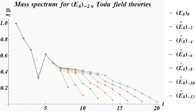
Figure 1: Mass ratios for the $r+2n$ particles in the $\left(\mathbf{\mathring{E}}_{8}\right)_{-2n}$-Toda field theories with almost stable noncrystallographic $H_{4}$ compound.

We observe the interesting feature that when comparing the masses with those of standard $E_{8}$-affine Toda field theory, four masses are especially stable and remain almost all identical irrespective of the value of $n$. These masses can be identified when recalling that folding the $E_{8}$-affine Toda field theory [4] leads to a grouping of the eight masses in the $E_{8}$-theory [19] into as two copies of four masses attributed to a theory based on the root space of noncrystallographic type $H_{4}$. One set is obtained from the other by a multiplication of the golden ration $\phi=(1+\sqrt{5})/2$. Normalizing the $E_{8}$- masses so that the largest takes on the value $1$, we have

$$m_{1} = 1,\quad~{}~{}~{}~{}\ \ \ \ m_{2}=2\sin(4\theta),\quad\ \ m_{3}=\frac{\cos\theta}{\phi\cos(4\theta)},\quad\ \ \ \ \ \ m_{4}=\frac{1}{2\phi\cos(4\theta)},\quad$$ (53)

$$m_{5} = \phi^{-1}m_{1},\quad m_{6}=\phi^{-1}m_{2},\quad~{}~{}~{}\ \ \ m_{7}=\phi^{-1}m_{3},\quad~{}~{}~{}\ \ \ \ \ \ \ m_{8}=\phi^{-1}m_{4},\quad$$ (54)

with $\theta=\pi/30$. We observe in figure 1 that the four $H_{4}$ masses in (53) are almost identical in all $(\mathbf{\mathring{E}}_{8}\mathbf{)}_{-2n}$-theories.

However, none of these theories, apart from $(\mathbf{\mathring{E}}_{8}\mathbf{)}_{0}$, passes the Painlevé integrability test. In all other cases the eigenvalues of the matrix $2D_{\mathbf{\mathring{g}}_{-(2n-1)}}K_{\mathbf{\mathring{g}}_{-(2n-1)}}$ are all non integer valued and sometimes negative. We find that $D_{\mathbf{\mathring{g}}_{1}}\equiv D_{\mathbf{E}_{8}}$ is positive definite, as is expected for the semi-simple case. We confirm in this case the relation (41) as $\mathop{\mathrm{i}nd}\left(2D_{\mathbf{E}_{8}}K_{\mathbf{E}_{8}}\right)=\mathop{\mathrm{i}nd}\left(K_{\mathbf{E}_{8}}\right)=8$. Moreover the eigenvalues factorize into $s_{i}(s_{i}+1)$ with $s_{i}=1$, $7$, $11$, $13$, $17$, $19$, $23$, $29$, corresponding to the $8$ exponents of $E_{8}$.

In contrast, the matrices $D_{\mathbf{\mathring{g}}_{-(2n-1)}}$ are negative definite for all values of $n\geq 1$. The $8+2n$ eigenvalues for $2D_{(\mathbf{\mathring{E}}_{8}\mathbf{)}_{-(2n-1)}}K_{(\mathbf{\mathring{E}}_{8}\mathbf{)}_{-(2n-1)}}$for $n=1,2,\ldots$ separate into $8+n$ negative and $n$ positive eigenvalues. The relation (41) is confirmed as

$$\mathop{\mathrm{i}nd}\left(-2D_{\mathbf{\mathring{g}}_{-(2n-1)}}K_{\mathbf{\mathring{g}}_{-(2n-1)}}\right)=\mathop{\mathrm{i}nd}\left(K_{\mathbf{\mathring{g}}_{-(2n-1)}}\right)=8,~{}\ \ \text{for }n=1,2,\ldots$$ (55)

Surprisingly the index of $K$ is preserved for all values of $n$. To make this plausible we list here the first characteristic polynomials $\det(K-\lambda\mathbb{I})=0$ for the Cartan matrix $K_{\mathbf{\mathring{g}}_{-(2n-1)}}$

$$\mathop{\mathrm{c}h}\left(K_{\mathbf{E}_{8}}\right) = \lambda^{8}-16\lambda^{7}+105\lambda^{6}-364\lambda^{5}+714\lambda^{4}-784\lambda^{3}+440\lambda^{2}-96\lambda+1,$$ (56)

$$\mathop{\mathrm{c}h}\left(K_{(\mathbf{\mathring{E}}_{8}\mathbf{)}_{-1}}\right) = \lambda^{10}-20\lambda^{9}+171\lambda^{8}-816\lambda^{7}+2379\lambda^{6}-4356\lambda^{5}+4949\lambda^{4}-3304\lambda^{3}$$

$$+1140\lambda^{2}-144\lambda-1,$$

$$\mathop{\mathrm{c}h}\left(K_{(\mathbf{\mathring{E}}_{8}\mathbf{)}_{-2}}\right) = \lambda^{12}-22\lambda^{11}+208\lambda^{10}-1100\lambda^{9}+3531\lambda^{8}-6892\lambda^{7}+7356\lambda^{6}$$

$$-1914\lambda^{5}-4872\lambda^{4}+5944\lambda^{3}-2626\lambda^{2}+388\lambda+1,$$

$$\mathop{\mathrm{c}h}\left(K_{(\mathbf{\mathring{E}}_{8}\mathbf{)}_{-4}}\right) = \lambda^{14}-24\lambda^{13}+249\lambda^{12}-1450\lambda^{11}+5103\lambda^{10}-10576\lambda^{9}+9896\lambda^{8}$$

$$+7088\lambda^{7}-31796\lambda^{6}+37074\lambda^{5}-17467\lambda^{4}-520\lambda^{3}+3050\lambda^{2}-636\lambda-1.$$

We observe that in each polynomial of the general form $\sum\nolimits_{i=1}^{8+2n}a_{i}\lambda^{i},$ the sequence of coefficients $a_{i}$ has exactly $8+n$ sign changes. Thus according to Descartes’ rule of signs, see e.g. [47], we have exactly $8+n$ positive real eigenvalues confirming the observation above. The factorization of these eigenvalues into $s_{i}(s_{i}+1)$ leads to the form $s_{i}=1/2+\lambda_{i}$ with $\lambda_{i}\in\mathbb{R}$ and $s_{i}=\kappa_{i}$ with $\kappa_{i}\in\mathbb{R}$, for the negative and positive eigenvalues, respectively.

We depict the eigenvalue spectra for some $\mathcal{L}_{{}_{(\mathbf{\mathring{E}}_{8}\mathbf{)}_{-2n}}}$-extended Lorentzian Toda field theory in figure 2.

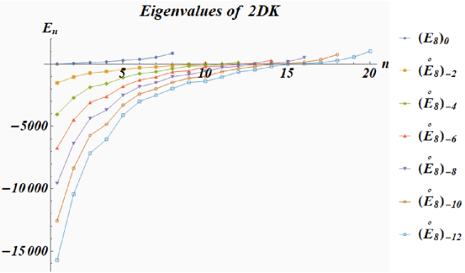
Figure 2: Eigenvalue spectra for the Painlevé matrix $2D_{\mathbf{\mathring{g}}_{-(2n-1)}}K_{\mathbf{\mathring{g}}_{-(2n-1)}}$.

As most of the eigenvalues are negative or non integer valued, the $\mathcal{L}_{{}_{(\mathbf{\mathring{E}}_{8}\mathbf{)}_{-2n}}}$-extended Lorentzian Toda field theory fail the Painlevé test and are therefore not integrable.

6.2 $\mathcal{L}_{(\mathbf{\mathring{g}}_{1}\mathbf{)}_{-2n}\diamond(\mathbf{\mathring{g}}_{2}\mathbf{)}_{-2m}}$-extended Lorentzian Toda field theory

This construction is based on a generalization of what is referred to in [33] as the symmetric fusion of two finite semisimple Lie algebras $g_{1}$ and $g_{2}$ by means of some Lorentzian roots in $\Pi^{1,1}$. Here we consider a root lattice of the form

$$\Lambda_{(\mathbf{\mathring{g}}_{1}\mathbf{)}_{1-2n}\diamond(\mathbf{\mathring{g}}_{2}\mathbf{)}_{1-2m}}=\Lambda_{(\mathbf{\mathring{g}}_{1}\mathbf{)}_{1-2n}}\oplus\Pi^{1,1}\oplus\Lambda_{(\mathbf{\mathring{g}}_{2}\mathbf{)}_{1-2m}}.$$ (60)

It is comprised of the $r_{1}+2n$ roots $\alpha_{i}$ with $i=1-2n,\ldots,r_{1}$ of $(\mathbf{\mathring{g}}_{1}\mathbf{)}_{1-2n}$, the $r_{2}+2m$ roots $\beta_{i}$ with $i=1-2m,\ldots,r_{2}$ of $(\mathbf{\mathring{g}}_{2}\mathbf{)}_{-2m}$ and two modified roots

$$\alpha_{-2n}=k_{n+1}-\sum\nolimits_{j=1-2n}^{r_{1}}n_{j}\alpha_{j},\qquad\beta_{-2m}=\bar{k}_{n+1}-\sum\nolimits_{j=-1-2m}^{r_{1}}n_{j}\beta_{j}$$

with $k_{n+1},\bar{k}_{n+1}\in\Pi^{1,1}$. The Lorentzian roots used in the construction of the $\alpha$ and $\beta$ roots are unrelated with mutual inner products equal to zero. They are labeled by $k_{i},\bar{k}_{i}$, $i=1,\ldots,n$ and $\ell_{i},\bar{\ell}_{i}$, $i=1,\ldots,m$, respectively. For $n=m=0$ this construction coincides with the one in [33] apart from a change of sign in the definition of $\beta_{0}$ where we added $\bar{k}$ instead of $-\bar{k}$ as in [33]. We explain the reason for our preferred choice below. The massive version is then constructed by adding a root $\gamma=-(k_{n+1}+\bar{k}_{n+1})$. Using the rules as stated above, the part of the Dynkin diagram where the $(\mathbf{\mathring{g}}_{1}\mathbf{)}_{-2n}$ and $(\mathbf{\mathring{g}}_{2}\mathbf{)}_{-2m}$ for $n\geq 1$, $m\geq 1$ are joined is:

The corresponding Cartan matrix is simply linking up the two affine Cartan matrices $K_{(\mathbf{\mathring{g}}_{1}\mathbf{)}_{-2n}}$ and $K_{(\mathbf{\mathring{g}}_{2}\mathbf{)}_{-2m}}$ as

$$K_{(\mathbf{\mathring{g}}_{1}\mathbf{)}_{-2n}\diamond(\mathbf{\mathring{g}}_{2}\mathbf{)}_{-2m}}=\left(\begin{array}[]{ccccccccc}&&&q_{1}&&0&0&\cdots&0\\ &K_{(\mathbf{\mathring{g}}_{1}\mathbf{)}_{1-2n}}&&\vdots&&\vdots&\vdots&&\vdots\\ &&&q_{r_{1}}&&0&0&&\vdots\\ q_{1}&\cdots&q_{r_{1}+2n}&0&-1&1&0&\cdots&0\\ &&&-1&2&-1&&&\\ 0&\cdots&0&1&-1&0&p_{r_{2}+2m}&\cdots&p_{1}\\ \vdots&&\vdots&0&&p_{r_{2}}&&&\\ \vdots&&\vdots&\vdots&&\vdots&&K_{(\mathbf{\mathring{g}}_{2}\mathbf{)}_{1-2m}}&\\ 0&\cdots&0&0&&p_{1}&&&\end{array}\right),$$ (61)

where $q_{s}:=\alpha_{-2n}\cdot\alpha_{s}$, $s=1,\ldots,r_{1}+2n$  and $p_{s}:=\beta_{-2m}\cdot\beta_{s}$, $s=1,\ldots,r_{2}+2m$.

We present now some examples for Lorentzian Toda field theories build from concrete algebras of this type of construction.

6.2.1 $(\mathbf{\mathring{E}}_{8})_{-2n}\diamond(\mathbf{\mathring{E}}_{8})_{-2n}$-Lorentzian Toda field theories

We start with $(\mathbf{\mathring{E}}_{8})_{0}\diamond(\mathbf{\mathring{E}}_{8})_{0}\equiv(\mathbf{E}_{8})_{0}\diamond(\mathbf{E}_{8})_{0}$ and take the same representation for the eight simple roots $\alpha_{i}$, $i=1,\ldots 8$ as defined in (51), but we enlarge the representation space from $10$ to $18$ dimensions by adding $8$ zero entries. The modified affine root $\alpha_{0}=k-\sum\nolimits_{j=1}^{8}n_{j}\alpha_{j}$ takes on the same form as in (51). Next we construct the roots for the second set of simple roots as $\beta_{i}^{j+10}=\alpha_{i}^{j}$, $i,j=1,\ldots 8$, and with all remaining entries $0$. The second modified affine root is constructed as $\beta_{0}=\bar{k}-\sum\nolimits_{j=1}^{8}n_{j}\beta_{j}$. The additional root $\gamma=-(k+\bar{k})$ has therefore nonvanishing entries $\gamma^{9}=-\gamma^{10}=-1$. The Dynkin diagram becomes in this case

Similarly we construct the Cartan matrix for the other members of the $(\mathbf{\mathring{E}}_{8})_{-2n}\diamond(\mathbf{\mathring{E}}_{8})_{-2n}$-series.

With a well defined root system and vanishing linear term we can compute the mass squared matrix as defined in (20). Once more we find that all eigenvalues of the mass squared matrix are positive. Taking the normalized square root of these eigenvalues, we depict the classical mass spectra for the first seven members of the $(\mathbf{\mathring{E}}_{8})_{-2n}\diamond(\mathbf{\mathring{E}}_{8})_{-2n}$-series in figure 3.

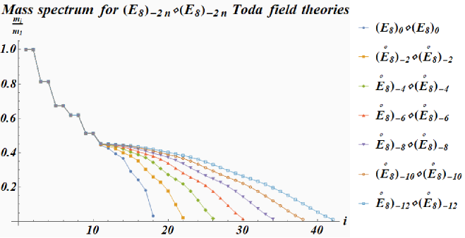
Figure 3: Mass ratios for the $18+2n$ particles in the $(\mathbf{\mathring{E}}_{8})_{-2n}\diamond(\mathbf{\mathring{E}}_{8})_{-2n}$-Lorentzian Toda field theory.

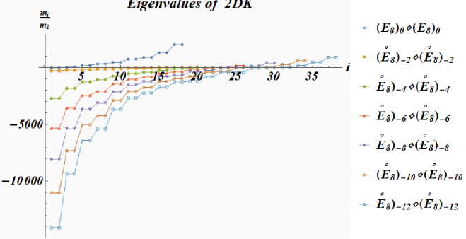
Figure 4: Real part of the eigenvalue spectra for the $2DK$-matrix for the $(\mathbf{\mathring{E}}_{8})_{-2n}\diamond(\mathbf{\mathring{E}}_{8})_{-2n}$-Lorentzian Toda field theory.

We note that all mass spectra in figure 3 are nondegenerate. Even though it may appear from the figure that some of the heaviest particles have the same mass, there is in fact always at least a very small difference not visible on the scale used in the figure. For the lighter particles in the spectrum the difference becomes more apparent. Splitting the particles into sets belonging to the left and right set of roots, $\alpha$ and $\beta$, respectively, and comparing with the mass spectrum of the affine $(\mathbf{E}_{8})_{0}$-theory, we observe that the mass spectrum of five heaviest particles is almost identical to the masses in the left and right set of roots.

Next we consider the eigenvalues of the Painlevé matrix. First we notice that the diagonal matrix $D_{(\mathbf{E}_{8})_{0}\diamond(\mathbf{E}_{8})_{0}}$ is positive definite and that the relation (41) holds with $\mathop{\mathrm{i}nd}\left(K_{(\mathbf{E}_{8})_{0}\diamond(\mathbf{E}_{8})_{0}}\right)=16$. It is these eigenvalue spectrum that motivates the choice for the sign in front of the Lorentzian roots in the definition of $\beta_{0}$. Choosing $-\bar{k}$ instead of $\bar{k}$ will not affect the mass spectrum, but it will reverse the sign in signature of the eigenvalues of $2DK$. However, this theory does not pass the Painlevé integrability test as the eigenvalues of the matrix $2DK$ are all non integer valued.

In contrast, for $(\mathbf{\mathring{E}}_{8})_{-2n}\diamond(\mathbf{\mathring{E}}_{8})_{-2n}$ with $n\geq 1$ the $D$-matrix is semi-definite with the four central diagonal entries $D_{(9+n\pm 1)(9+n\pm 1)}$, $D_{(9+n\pm 2)(9+n\pm 2)}$ being positive and the remaining negative. Defining a reduced $D$-matrix as $\hat{D}$ by setting the positive entries to zero we find a reduced version of (41) as $\mathop{\mathrm{i}nd}(-2\hat{D}K)=\mathop{\mathrm{i}nd}(K)=16$. None of the theories in this series passes the Painlevé integrability test as the eigenvalues of the matrix $2DK$ are not only all non integer valued or negative, but in addition some of the eigenvalues occur in complex conjugate pairs. We depict the real eigenvalues in figure 4.

We observe that the “almost degeneracy is roughly preserved for the six heaviest particles.

7 Conclusions

We have introduced various types of construction principles for conformal, i.e. massless, and massive versions of Toda field theories based on roots defined on Lorentzian lattices. We carried out a detailed Painlevé integrability test, that established that these theories are in general not integrable. Nonetheless, the theories possess well defined classical mass spectra and inherit some of the features of their integrable reductions. For instance, part of the mass spectrum of the $(\mathbf{\mathring{E}}_{8}\mathbf{)}_{-2n}$-theories consists of the four masses of the noncrystallographic $H_{4}$-theory obtained by folding the integrable affine $\mathbf{E}_{8}$-theory. Remarkably, these masses are only slightly changed for all values of $n$, so that we may view this feature as a remnant that survives the perturbation of the integrable system.

Evidently there are many interesting routes for further investigations left. We have only presented here some of the examples of algebras we have investigated. It would be interesting to extract more generic features from those and develop an algebraically independent formulation and treatment for them similar to their integrable counterparts. It is clear from the above, that there are also more options for possible construction principles that can be explored further. Of course also standard calculations, such as mass renormalization for these theories or the study of flows between models can be carried out.

Acknowledgments: SW is supported by a City, University of London Research Fellowship.

References

- [1] M. Toda, Studies of a non-linear lattice, Physics Reports 18(1), 1–123 (1975).
- [2] O. I. Bogoyavlensky, On perturbations of the periodic Toda lattice, Comm. in Math. Phys. 51(3), 201–209 (1976).
- [3] H. Yoshida, Integrability of generalized Toda lattice systems and singularities in the complex t-plane, in Nonlinear integrable systems-Classical theory and Quantum theory, pages 273–289, World Science Publishing Co Singapore, 1983.
- [4] A. Fring and C. Korff, Affine Toda field theories related to Coxeter groups of noncrystallographic type, Nucl. Phys. B 729(3), 361–386 (2005).
- [5] T. L. Curtright and C. B. Thorn, Conformally invariant quantization of the Liouville theory, Phys. Rev. Lett. 48(19), 1309 (1982).
- [6] P. Mansfield, Light-cone quantisation of the Liouville and Toda field theories, Nucl. Phys. B 222(3), 419–445 (1983).
- [7] H. W. Braden, E. Corrigan, P. E. Dorey, and R. Sasaki, Affine Toda field theory and exact S matrices, Nucl. Phys. B338, 689–746 (1990).
- [8] A. Fring, H. C. Liao, and D. Olive, The mass spectrum and coupling in affine Toda theories, Phys. Lett. B 266, 82–86 (1991).
- [9] A. Mikhailov, M. Olshanetsky, and A. Perelomov, Two-dimensional generalized Toda lattice, Comm. Math. Phys. 79, 473–488 (1981).
- [10] M. A. Olshanetsky and A. M. Perelomov, Quantum integrable systems related to Lie algebras, Phys. Rept. 94, 313–404 (1983).
- [11] G. Wilson, The modified Lax and two-dimensional Toda lattice equations associated with simple Lie algebras, Ergodic Theory and Dynamical Systems 1(3), 361–380 (1981).
- [12] D. I. Olive and N. Turok, Local conserved densities and zero curvature conditions for Toda lattice field theories, Nucl. Phys. B257, 277 (1985).
- [13] A. N. Leznov and M. V. Savelev, Two-dimensional exactly and completely integrable dynamical systems (monopoles, instantons, dual models, relativistic strings, Lund Regge model, genalised Toda lattice et.), Commun. Math. Phys. 89, 59 (1983).
- [14] T. Hollowood, Solitons in affine Toda field theory, Nucl. Phys. B384, 523–540 (1992).
- [15] H. Aratyn, C. P. Constantinidis, L. A. Ferreira, J. F. Gomes, and A. H. Zimerman, Hirota’s solitons in the affine and the conformal affine Toda models, Nucl. Phys. B 406, 727–770 (1993).
- [16] D. I. Olive, N. Turok, and J. W. R. Underwood, Solitons and the energy momentum tensor for affine Toda theory, Nucl. Phys. B401, 663–697 (1993).
- [17] A. Fring, P. R. Johnson, M. A. C. Kneipp, and D. I. Olive, Vertex operators and soliton time delays in affine Toda field theory, Nuclear Physics B 430, 597–614 (1994).
- [18] A. Arinshtein, V. Fateev, and A. Zamolodchikov, Quantum S-matrix of the (1 + 1)-dimensional Toda chain, Phys. Lett. B87, 389–392 (1979).
- [19] A. B. Zamolodchikov, Integrals of motion and S-matrix of the (scaled) Ising model with magnetic field, Int. J. of Mod. Phys. A 4(16), 4235–4248 (1989).
- [20] P. Christe and G. Mussardo, Integrable Sytems away from criticality: The Toda field theory and S matrix of the tricritical Ising model, Nucl. Phys. B330, 465 (1990).
- [21] P. Christe and G. Mussardo, Elastic S-matrices in (1+ 1) dimensions and Toda field theories, Int. J. Mod. Phys. A5, 4581–4628 (1990).
- [22] P. Dorey, Root systems and purely elastic S-matrices, Nucl. Phys. B 358(3), 654–676 (1991).
- [23] A. Fring and D. I. Olive, The Fusing rule and the scattering matrix of affine Toda theory, Nucl. Phys. B379, 429–447 (1992).
- [24] C. Destri and H. J. de Vega, New exact results in affine Toda field theories: Free energy and wave function renormalizations, Nucl. Phys. B358, 251–294 (1991).
- [25] T. Oota, q-deformed Coxeter element in non-simply laced affine Toda field theories, Nucl. Phys. B504, 738–752 (1997).
- [26] A. Fring, C. Korff, and B. J. Schulz, On the universal representation of the scattering matrix of affine Toda field theory, Nucl. Phys. B567, 409–453 (2000).
- [27] D. Bernard and A. LeClair, Quantum group symmetries and non-local currents in 2D QFT, Comm. in Math. Phys. 142(1), 99–138 (1991).
- [28] R. W. Gebert, S. Mizogushi, and T. Inami, Toda field theories associated with hyperbolic Kac-Moody algebra Painleve properties and W algebras, Int. J. of Mod Phys. A 11(31), 5479–5493 (1996).
- [29] L. Carbone, S. Chung, L. Cobbs, R. McRae, D. Nandi, Y. Naqvi, and D. Penta, Classification of hyperbolic Dynkin diagrams, root lengths and Weyl group orbits, J. of Phys. A: Math. and Theor. 43(15), 155209 (2010).
- [30] T. Damour, M. Henneaux, and H. Nicolai, E10 and a small tension expansion of M theory, Phys. Rev. Lett. 89(22), 221601 (2002).
- [31] H. Nicolai and T. Fischbacher, Low level representations for E10 and E11, Cont. Math 343, 191 (2004).
- [32] R. Borcherds, Generalized Kac-Moody algebras, Journal of Algebra 115(2), 501–512 (1988).
- [33] M. R. Gaberdiel, D. I. Olive, and P. C. West, A class of Lorentzian Kac–Moody algebras, Nuclear Physics B 645, 403–437 (2002).
- [34] A. Fring and S. Whittington, n-Extended Lorentzian Kac–Moody algebras, Letters in Mathematical Physics , 1–22 (2020).
- [35] G. Delfino, G. Mussardo, and P. Simonetti, Non-integrable quantum field theories as perturbations of certain integrable models, Nucl. Phys. B 473(3), 469–508 (1996).
- [36] O. Babelon and L. Bonora, Conformal affine sl2 Toda field theory, Phys. Lett. B 244(2), 220–226 (1990).
- [37] H. Aratyn, L. A. Ferreira, J. F. Gomes, and A. H. Zimerman, Kac-Moody construction of Toda type field theories, Phys. Lett. B 254(3-4), 372–380 (1991).
- [38] P. Painlevé, Mémoire sur les équations différentielles dont l’intégrale générale est uniforme, Bull. Soc. Math. France 28, 201–261 (1900).
- [39] M. Ablowitz, A. Ramani, and H. Segur, A connection between nonlinear evolution equations and ordinary differential equations of P-type. II, J. Math. Phys. 21, 1006–1015 (1980).
- [40] J. Weiss, M. Tabor, and G. Carnevale, The Painlevé property for partial differential equations, J. Math. Phys. 24, 522–526 (1983).
- [41] N. Joshi and J. Peterson, A method of proving the convergence of the Painleve expansions of partial differential equations, Nonlinearity 7, 595–602 (1994).
- [42] B. Grammaticos and A. Ramani, Integrability- and How to detect it, Lect. Notes Phys. 638, 31–94 (2004).
- [43] H. Nicolai and D. I. Olive, The principal SO (1, 2) subalgebra of a hyperbolic Kac–Moody algebra, Lett. in Math. Phys. 58(2), 141–152 (2001).
- [44] J. B. Carrell, Fundamentals of linear algebra, The University of British Columbia (2005).
- [45] L. Frappat, A. Sciarrino, and P. Sorba, Structure of basic Lie superalgebras and of their affine extensions, Comm. in Math. Phys. 121(3), 457–500 (1989).
- [46] J. Balog, L. Feher, L. O’Raifeartaigh, P. Forgacs, and A. Wipf, Toda theory and W-algebra from a gauged WZNW point of view, Annals of Physics 203(1), 76–136 (1990).
- [47] B. Anderson, J. Jackson, and M. Sitharam, Descartes’ rule of signs revisited, The American Mathematical Monthly 105(5), 447–451 (1998).