OU-HEP-200430

A string landscape guide to soft SUSY breaking terms
Howard Baer¹, Vernon Barger², Shadman Salam¹
and Dibyashree Sengupta^1
1Homer L. Dodge Department of Physics and Astronomy, University of Oklahoma, Norman, OK 73019, USA
²Department of Physics, University of Wisconsin, Madison, WI 53706 USA

We examine several issues pertaining to statistical predictivity of the string theory landscape for weak scale supersymmetry (SUSY). We work within a predictive landscape wherein super-renormalizable terms scan while renormalizable terms do not. We require stringy naturalness wherein the likelihood of values for observables is proportional to their frequency within a fertile patch of landscape including the MSSM as low energy effective theory with a pocket-universe value for the weak scale nearby to its measured value in our universe. In the string theory landscape, it is reasonable that the soft terms enjoy a statistical power-law draw to large values, subject to the existence of atoms as we know them (atomic principle). We argue that gaugino masses, scalar masses and trilinear soft terms should each scan independently. In addition, the various scalars should scan independently of each other unless protected by some symmetry. The expected non-universality of scalar masses– once regarded as an undesirable feature– emerges as an asset within the context of the string landscape picture. In models such as heterotic compactifications on Calabi-Yau manifolds, where the tree-level gauge kinetic function depends only on the dilaton, then gaugino masses may scale mildly, while scalar masses and A-terms, which depend on all the moduli, may scale much more strongly leading to a landscape solution to the SUSY flavor and CP problems in spite of non-diagonal Kähler metrics. We present numerical results for Higgs and sparticle mass predictions from the landscape within the generalized mirage mediation SUSY model and discuss resulting consequences for LHC SUSY and WIMP dark matter searches.

1 Introduction

The laws of physics as we know them are beset with several fine-tuning problems that can be interpreted as omissions in our present level of understanding. It is hoped that these gaps may be filled by explanations requiring additional input from physics beyond the Standard Model (SM). One of these, the strong CP problem, is solved via the introduction of a global Peccei-Quinn (PQ) symmetry and its concomitant axion $a$. Another, the gauge hierarchy or Higgs mass problem, is solved via the introduction of weak scale supersymmetry wherein the SM Higgs mass quadratic divergences are rendered instead to be more mild log divergences. In this latter case, the non-discovery of SUSY particles at LHC has led to concerns of a Little Hierarchy problem (LHP), wherein one might expect the weak energy scale $m_{weak}\sim m_{W,Z,h}$ to be in the multi-TeV range rather than at its measured value $m_{weak}\simeq 100$ GeV. A third fine-tuning problem is the cosmological constant (CC) problem, wherein one expects the cosmological constant $\Lambda\sim m_{P}^{2}\sim 6\times 10^{54}$ eV² as opposed to its measured value $\Lambda\simeq 4.33\times 10^{-66}$ eV². The most plausible solution to the CC problem is Weinberg’s anthropic solution[1, 2]: the value of $\Lambda$ ought to be as natural as possible subject to generating a pocket universe whose expansion rate is not so rapid that structure in the form of galaxy condensation should not occur (this is called the structure principle).

The anthropic CC solution emerges automatically from the string theory landscape of (metastable) vacua[3] wherein each vacuum solution generates a different low energy effective field theory (EFT) and hence apparently different laws of physics (gauge groups, matter content, $\Lambda$, $m_{weak}$ etc.). A commonly quoted value for the number of flux vacua in IIB string theory is $N_{vac}\sim 10^{500}$[4]. If the CC is distributed (somewhat) uniformly across its (anthropic) range of values, then it may not be surprising that we find ourselves in a pocket universe with $\Lambda\sim 10^{-120}m_{P}^{2}$ since if it were much bigger, we wouldn’t be here. The situation is not dissimilar to the human species finding itself fortuitously on a moderate size planet a moderate distance from a stable, class-M star: the remaining vast volume of the solar system where we might also find ourselves is inhospitable to liquid water and life as we know it and we would never have evolved anywhere else.

An essential element to allow Weinberg’s reasoning to be predictive is that in the subset of pocket universes with varying cosmological constant, the remaining laws of physics as encoded in the Standard Model stay the same: only $\Lambda$ is scanned by the multiverse. Such a subset ensemble of pocket universes is sometimes referred to as a fertile patch. Arkani-Hamed et al.[5] (ADK) argue that only super-renormalizable Lagrangian terms should scan in the multiverse while renormalizable terms such as gauge and Yukawa couplings will have their values fixed by dynamics. In the case of an ensemble of SM-like pocket universes with the same gauge group and matter content, with Higgs potential given by

$$V_{SM}=-\mu_{SM}^{2}\phi^{\dagger}\phi+\lambda(\phi^{\dagger}\phi)^{2},$$ (1)

(where $\phi$ is the usual SM Higgs doublet) then just $\mu_{SM}$ and $\Lambda$ should scan. This would then allow for the possibility of an anthropic solution to the gauge hierarchy problem in that the value of $\mu_{SM}$ (wherein $m_{h}^{2}(tree)=2\mu_{SM}^{2}$) would be anthropically selected to cancel off the (regularized) quadratic divergences. Such a scenario is thought to offer an alternative to the usual application of naturalness, which instead would require the advent of new physics at or around the weak scale.

Here, when we refer to naturalness of a physical theory, we refer to

practical naturalness: wherein each independent contribution to any physical observable is required to be comparable to or less than its measured value.

For instance, practical naturalness was successfully used by Gaillard and Lee to predict the value of the charm quark mass based on contributions to the measured value of the $K_{L}-K_{S}=\Delta m_{K}$ mass difference[6]. In addition, it can be claimed that perturbative calculations in theories such as QED are practically natural (up to some effective theory cutoff $\Lambda_{QED}$). While divergent contributions to observables appear at higher orders, these are dependent quantities: and once dependent quantities are combined, then higher order contributions to observables are comparable to or less than their measured values. Thus, we understand the concept of practical naturalness and the supposed predictivity of a theory to be closely aligned.

To place the concept of naturalness into the context of the landscape of string theory vacua, Douglas has proposed the notion of stringy naturalness[7]:

stringy naturalness: the value of an observable ${\cal O}_{2}$ is more natural than a value ${\cal O}_{1}$ if more phenomenologically viable vacua lead to ${\cal O}_{2}$ than to ${\cal O}_{1}$.

If we apply this definition to the cosmological constant, then phenomenologically viable is interpreted in an anthropic context in that we must veto vacua which do not allow for structure formation (in the form of galaxy condensation). Out of the remaining viable vacua, we would expect $\Lambda$ to be nearly as large as anthropically possible since there is more volume in parameter space for larger values of $\Lambda$. Such reasoning allowed Weinberg to predict the value of $\Lambda$ to within a factor of a few of its measured value more than a decade before its value was determined from experiment[1, 2]. The stringy naturalness of the cosmological constant is but one example of what ADK call living dangerously: the values of parameters scanned by the landscape are likely to be selected to be just large enough, but not so large as to violate some fragile feature of the world we live in (such as in this case the existence of galaxies).

The minimal supersymmetric standard model (MSSM) is touted as a natural solution to the gauge hierarchy problem. This is because in the MSSM log divergent contributions to the weak scale are expected to be comparable to the weak scale for soft SUSY breaking terms $\sim m_{weak}$. But is the MSSM also more stringy natural than the SM? The answer given in Ref. [8] is yes. For the case of the SM valid up to some energy scale $\Lambda_{SM}\gg m_{weak}$, then there is only an exceedingly tiny (fine-tuned) range of $\mu_{SM}^{2}$ values which allow for pocket-universe $m_{weak}^{PU}\sim m_{weak}(measured)$. In contrast, within the MSSM there is a very broad range of superpotential $\mu$ values which allow for $m_{weak}^{PU}\sim m_{weak}(measured)$, provided other contributions to the weak scale are also comparable to $m_{weak}(measured)$ (as bourne out by Fig’s 2 and 3 of Ref. [8]). For the MSSM, the pocket universe value of the weak scale is given by

$$\frac{(m_{Z}^{PU})^{2}}{2}=\frac{m_{H_{d}}^{2}+\Sigma_{d}^{d}-(m_{H_{u}}^{2}+\Sigma_{u}^{u})\tan^{2}\beta}{\tan^{2}\beta-1}-\mu^{2}\simeq-m_{H_{u}}^{2}-\Sigma_{u}^{u}-\mu^{2}$$ (2)

where the value of $\mu$ is specified by whatever solution to the SUSY $\mu$ problem is invoked[9]. (Here, $m_{H_{u}}^{2}$ and $m_{H_{d}}^{2}$ are the Higgs field soft squared-masses and the $\Sigma_{d}^{d}$ and $\Sigma_{u}^{u}$ contain over 40 loop corrections to the weak scale (expressions can be found in the Appendix to Ref. [10])). Thus, the pocket universe value for the weak scale is determined by the soft SUSY breaking terms and the SUSY-preserving $\mu$ parameter. If the landscape of string vacua include as low energy effective theories both the MSSM and the SM, then far more vacua with a natural SUSY EFT should lead to $m_{weak}^{PU}\sim m_{weak}(measured)$ as compared to vacua with the SM EFT where $\Lambda_{SM}\gg m_{weak}$. In this vein, unnatural SUSY models such as high scale SUSY where $m_{soft}\gg m_{weak}$ should be rare occurrences on the landscape as compared to natural SUSY.

Douglas has also proposed a functional form for the dependence of the distribution of string theory vacua on the SUSY breaking scale[11]. The form expected for gravity/moduli mediation is given by

$$dN_{vac}(m_{hidden}^{2},m_{weak},\Lambda)=f_{SUSY}\cdot f_{EWFT}\cdot f_{CC}\cdot dm_{hidden}^{2}$$ (3)

where the hidden sector SUSY breaking scale $m_{hidden}^{4}=\sum_{i}|F_{i}|^{2}\,+\,\frac{1}{2}\sum_{\alpha}D^{2}_{\alpha}$ is a mass scale associated with the hidden sector (and usually in SUGRA-mediated models it is assumed $m_{hidden}\sim 10^{12}$ GeV such that the gravitino gets a mass $m_{3/2}\sim m_{hidden}^{2}/m_{P}$). Consequently, in gravity-mediation then the visible sector soft terms $m_{soft}\sim m_{3/2}$. As noted by Susskind[12] and Douglas[4], the scanning of the cosmological constant is effectively independent of the determination of the SUSY breaking scale so that $f_{CC}\sim\Lambda/m_{string}^{4}$.

Another key observation from examining flux vacua in IIB string theory is that the SUSY breaking $F_{i}$ and $D_{\alpha}$ terms are likely to be uniformly distributed– in the former case as complex numbers while in the latter case as real numbers. Then one expects the following distribution of supersymmetry breaking scales

$$f_{SUSY}(m_{hidden}^{2})\,\sim\,(m^{2}_{hidden})^{2n_{F}+n_{D}-1}$$ (4)

where $n_{F}$ is the number of $F$-breaking fields and $n_{D}$ is the number of $D$-breaking fields in the hidden sector. Even for the case of just a single $F$-breaking term, then one expects a linear statistical draw towards large soft terms; $f_{SUSY}\sim m_{soft}^{n}$ where $n=2n_{F}+n_{D}-1$ and in this case where $n_{F}=1$ and $n_{D}=0$ then $n=1$. For SUSY breaking contributions from multiple hidden sectors, as typically expected in string theory, then $n$ can be much larger, with a consequent stronger pull towards large soft breaking terms.

An initial guess for $f_{EWFT}$, the (anthropic) fine-tuning factor, was $m_{weak}^{2}/m_{soft}^{2}$ which would penalize soft terms which were much bigger than the weak scale. This form is roughly suggested by fine-tuning measures such as $\Delta_{EW}$ where

$$\Delta_{EW}=|maximal\ contribution\ to\ RHS\ of\ Eq.~{}\ref{eq:mzs}|/(m_{Z}^{2}/2)$$ (5)

where then $f_{EWFT}\sim\Delta_{EW}^{-1}$.

This ansatz fails on several points[13].

• Many soft SUSY breaking choices will land one into charge-or-color breaking (CCB) minima of the EW scalar potential. Such vacua would likely not lead to a livable universe and should be vetoed rather than penalized.

• Other choices for soft terms may not even lead to EW symmetry breaking (EWSB). For instance, if $m_{H_{u}}^{2}(\Lambda)$ is too large, then it will not be driven negative to trigger spontaneous EWSB. These possibilities, labelled as no-EWSB vacua, should also be vetoed.

• In the event of appropriate EWSB minima, then sometimes larger high scale soft terms lead to more natural weak scale soft terms. For instance, 1. if $m_{H_{u}}^{2}(\Lambda)$ is large enough that EWSB is barely broken, then $|m_{H_{u}}^{2}(weak)|\sim m_{weak}^{2}$ (see Fig. 3 of Ref. [14]). Likewise, 2. if the trilinear soft breaking term $A_{t}$ is big enough, then there is large top squark mixing and the $\Sigma_{u}^{u}(\tilde{t}_{1,2})$ terms enjoy large cancellations, rendering them $\sim m_{weak}^{2}$[15, 10]. The same large $A_{t}$ values lift the Higgs mass $m_{h}$ up to the 125 GeV regime. Also, 3. as first/second generation soft masses are pulled to the tens of TeV regime, then two-loop RGE effects actually suppress third generation soft terms so that SUSY may become more natural[16].

If one assumes a solution to the SUSY $\mu$ problem[9], which fixes the value of $\mu$ so that it can no longer be freely fine-tuned to fix $m_{Z}$ at its measured value, then once the remaining SUSY model soft terms are set, one obtains a pocket-universe value of the weak scale as an output: e.g $m_{Z}^{PU}\neq m_{Z}(measured)$. Based on nuclear physics calculations by Agrawal et al.[17, 18], a pocket universe value of $m_{weak}^{PU}$ which deviates from our measured value by a factor 2-5 is likely to lead to an unlivable universe as we understand it. Weak interactions and fusion processes would be highly suppressed and even complex nuclei could not form. This would be a violation of the atomic principle: that atoms as we know them seem necessary to support observers. This is another example of living dangerously: the pull towards large soft terms tend to pull the value of $m_{weak}^{PU}$ up in value, but must stop short of a factor of a few times our measured weak scale lest one jeopardize the existence of atoms as we know them. We will adopt a conservative value that the weak scale should not deviate by more than a factor four from its measured value. This corresponds to a value of the fine-tuning measure $\Delta_{EW}\lesssim 30$. Thus, for our final form of $f_{EWFT}$ we will adopt[13]

$$f_{EWFT}=\Theta(30-\Delta_{EW})$$ (6)

while also vetoing CCB and no-EWSB vacua.

The above Eq. 3 has been used to generate statistical distributions for Higgs and sparticle masses as expected from the string theory landscape for various assumed values of $n=0-4$ and for assumed gravity-mediation model NUHM3[13] and also for generalized mirage mediation[19]. For values $n>0$, then there is a statistical pull on $m_{h}$ to a peak at $m_{h}\simeq 125$ GeV in agreement with the measured value of the Higgs boson mass. Also, for $n\geq 1$, then typically the gluino gets pulled to mass values $m_{\tilde{g}}\sim 4\pm 2$ TeV, i.e. pulled above LHC mass limits. The lighter top squark is pulled to values $m_{\tilde{t}_{1}}\sim 2\pm 1$ TeV while higgsinos remain in the $m_{\widetilde{\chi}^{0}_{1,2},\widetilde{\chi}^{\pm}_{1}}\sim 100-350$ GeV range. Since gaugino masses are pulled to large values, the neutralino mass gap decreases to $m_{\widetilde{\chi}^{0}_{2}}-m_{\widetilde{\chi}^{0}_{1}}\sim 3-5$ GeV, making higgsino pair production $pp\rightarrow\widetilde{\chi}^{0}_{1}\widetilde{\chi}^{0}_{2},\ \widetilde{\chi}^{\pm}_{1}\widetilde{\chi}^{0}_{2}$ very difficult to see at LHC via the soft opposite-sign dilepton signature from $\widetilde{\chi}^{0}_{2}\rightarrow\widetilde{\chi}^{0}_{1}\ell^{+}\ell^{-}$ decay[20]. Thus, this simple statistical model of the string landscape correctly predicts both the mass of the lightest Higgs boson and the fact that LHC sees so far no sign of superparticles. And since first/second generation matter scalars are pulled towards a common upper bound in the $20-40$ TeV range, it also predicts only slight violations of FCNC and CP-violating processes due to a mixed decoupling/quasi-degeneracy solution to the SUSY flavor and CP problems[16].

Our goal in this paper is to investigate several issues of soft SUSY breaking terms relevant for the landscape. The first issue is addressed in Sec. 2: which soft terms should scan on the landscape and why. The second issue is: of the soft terms which ought to scan, should they scan with a common exponent $n$, or are there cases where different soft terms would be drawn more strongly to large values than others: i.e. should different $n$ values apply to different soft terms, depending on the string model? We address both these issues in Sec. 2. Then in Sec. 3, we apply what we have learned in Sec. 2 to examine how stringy natural are different regions of model parameter space, as compared to choosing a common exponent $n$ for all scanning soft terms. Since in the landscape picture many of the soft terms are drawn into the tens-of-TeV range, we expect a comparable value of gravitino mass $m_{3/2}$, but with TeV scale gauginos. In such a case, we expect comparable gravity- and anomaly-mediated contributions to soft terms so that we present our numerical results within the generalized mirage mediation model GMM^′[21]. Some discussion on implications for LHC searches along with overall conclusions are presented in Sec. 4.

2 Soft SUSY breaking terms

2.1 Soft terms in the low energy EFT

In string theory, the starting point is the 10/11 dimensional UV complete string theory. One then writes the corresponding 10/11 dimensional effective supergravity (SUGRA) theory by integrating out KK modes and other superheavy states. Compactification of the 10/11 dimensional SUGRA on a Calabi-Yau manifold (to preserve $N=1$ SUSY in the ensuing $4-d$ theory) leads to a $4-d$ SUGRA theory containing visible sector fields plus a plethora (of order hundreds) of gravitationally coupled moduli fields, grouped according to complex structure moduli $U_{j}$ and Kähler moduli $T_{i}$. In accord with Ref’s [22, 23], we will include the dilaton field $S$ amongst the set of moduli. In simple II-B string models, the $U_{j}$ moduli are stabilized by flux while the Kähler moduli are stabilized by various non-perturbative effects[24, 25]. In explicit constructions, only one or a few Kähler moduli are assumed while realistically of order $\sim 100$ may be expected. The moduli stabilization allows in principle their many vevs to be determined, which then determines the many parameters of the effective theory. For simplicity, here we will assume the visible sector fields $C_{\alpha}$ consist of the usual MSSM fields. We will also assume that the moduli $S,\ T_{i},\ U_{j}$ form the hidden sector of the $4-d$ theory, and provide the required arena for SUSY breaking. From this framework, we will then draw conclusions as to precisely which soft terms will scan independently within the landscape, and how they are selected for by the power-law formula $f_{SUSY}\sim m_{soft}^{n}$. While many insights into moduli stabilization were made for the case of II-B string theory, we expect similar mechanisms to occur for other string models (heterotic, etc) since the various theories are all related by their duality relations.

The $4-d$, $N=1$ supergravity Lagrangian is determined by just two functions that depend on the chiral superfields $\phi_{M}$ of the model: the real gauge invariant Kähler function $G(\phi_{M},\phi_{M}^{*})=K(\phi_{M},\phi_{M}^{*})+\log|W(\phi_{M})|^{2}$ (with $K$ being the real valued Kähler potential and $W$ the holomorphic superpotental) and the holomorphic gauge kinetic function $f_{a}(\phi_{M})$. This is presented in units where the reduced Planck scale $m_{P}=M_{Pl}/\sqrt{8\pi}=1$. The chiral superfields of SUGRA $\phi_{M}$ are distinguished according to visible sector fields $C^{\alpha}$ and hidden sector fields $h_{m}$. Following [26, 22, 23], first we expand the superpotential as a power series in terms of the visible sector fields:

$$W=\hat{W}(h_{m})+\frac{1}{2}\mu_{\alpha\beta}(h_{m})C^{\alpha}C^{\beta}+\frac{1}{6}Y_{\alpha\beta\gamma}(h_{m})C^{\alpha}C^{\beta}C^{\gamma}+\cdots$$ (7)

while the expansion for the Kähler potential is

$$K=\hat{K}(h_{m},h_{m}^{*})+\tilde{K}_{\bar{\alpha},\beta}(h_{m},h_{m}^{*})C^{*\bar{\alpha}}C^{\beta}+\left[\frac{1}{2}Z_{\alpha\beta}(h_{m},h_{m}^{*})C^{\alpha}C^{\beta}+h.c.\right]+\cdots$$ (8)

and where the various coefficients of expansion are to-be-determined functions of the hidden sector fields $h_{m}$. In the above, Greek indices correspond to visible sector fields while lower-case latin indices correspond to hidden sector fields. Upper case latin indices correspond to general chiral superfields.

The $F$-part of the scalar potential is given by

$$V(\phi_{M},\phi_{M}^{*})=e^{G}\left(G_{M}K^{M\bar{N}}G_{\bar{N}}-3\right)\\ =\left(\bar{F}^{\bar{N}}K_{\bar{N}M}F^{M}-3e^{G}\right)$$ (9)

If some of the fields $h_{m}$ develops vevs such that at least one of the auxiliary fields $F^{m}=e^{G/2}\hat{K}^{m\bar{n}}G_{\bar{n}}\neq 0$, then SUGRA is spontaneously broken. The gravitino gains a mass $m_{3/2}=e^{G/2}$ while soft SUSY breaking terms are generated. The soft terms are obtained from the general $4-d$, $N=1$ supergravity Lagrangian[27] by replacing the hidden fields $h_{m}$ and their $F_{m}$-terms by their vevs and then taking the flat limit wherein $m_{P}\rightarrow\infty$ while keeping $m_{3/2}$ fixed. One is then left with the low energy EFT which consists of a renormalizable global SUSY Lagrangian augmented by soft SUSY breaking terms.

The canonically normalized gaugino masses are given by

$$M_{a}=\frac{1}{2}(Re\ f_{a})^{-1}F^{m}\partial_{m}f_{a}$$ (10)

The unnormalized Yukawa couplings are given by

$$Y^{\prime}_{\alpha\beta\gamma}=\frac{\hat{W}^{*}}{|\hat{W}|}e^{\hat{K}/2}Y_{\alpha\beta\gamma}$$ (11)

while the superpotential $\mu$ terms is given by

$$\mu^{\prime}_{\alpha\beta}=\frac{\hat{W}^{*}}{|\hat{W}|}e^{\hat{K}/2}\mu_{\alpha\beta}+m_{3/2}Z_{\alpha\beta}-\bar{F}^{\bar{m}}\partial_{\bar{m}}Z_{\alpha\beta}$$ (12)

The scalar potential is expanded as

$$V_{soft}=m^{\prime 2}_{\bar{\alpha}\beta}C^{*\bar{\alpha}}C^{\beta}+\left(\frac{1}{6}A^{\prime}_{\alpha\beta\gamma}C^{\alpha}C^{\beta}C^{\gamma}+\frac{1}{2}B^{\prime}_{\alpha\beta}C^{\alpha}C^{\beta}+h.c.\right)$$ (13)

with unnormalized soft terms give by

$$m^{\prime 2}_{\bar{\alpha}\beta}=\left(m_{3/2}^{2}+V_{0}\right)\tilde{K}_{\bar{\alpha}\beta}-\bar{F}^{\bar{m}}\left(\partial_{\bar{m}}\partial_{n}\tilde{K}_{\bar{\alpha}\beta}-\partial_{\bar{m}}\tilde{K}_{\bar{\alpha}\gamma}\tilde{K}^{\gamma\bar{\delta}}\partial_{n}\tilde{K}_{\bar{\delta}\beta}\right)F^{n}$$ (14)

and

$$A^{\prime}_{\alpha\beta\gamma}=\frac{\hat{W}^{*}}{|\hat{W}|}e^{\hat{K}/2}F^{m}\left[\hat{K}_{m}Y_{\alpha\beta\gamma}+\partial_{m}Y_{\alpha\beta\gamma}-\left(\tilde{K}^{\delta\bar{\rho}}\partial_{m}\tilde{K}_{\bar{\rho}\alpha}Y_{\delta\beta\gamma}+(\alpha\leftrightarrow\beta)+(\alpha\leftrightarrow\gamma)\right)\right].$$ (15)

We shall not need the (rather lengthy) expression for $B^{\prime}_{\alpha\beta}$.

2.2 Implications for the landscape

2.2.1 Gaugino masses

The normalized gaugino mass soft terms are given in Eq. 10 where $Re(f_{a})=1/g_{a}^{2}$. For non-zero gaugino masses, then the gauge kinetic function $f_{a}$ must be a non-trivial function of the moduli fields. In most $4-d$ string constructs, then $f_{a}$ is taken as $k_{a}S$ where $k_{a}$ is the Kac-Moody level of the gauge factor. This form of the gauge kinetic function leads to universal gaugino masses which require SUSY breaking in the dilaton field $S$. The remaining moduli can enter $f_{a}$ at the loop level and lead to non-universal gaugino masses. If the moduli-contribution to $M_{a}$ is comparable to the dilaton contribution, then one might expect non-universal gaugino masses, but otherwise the non-universality would be a small effect. If the gaugino masses are dominantly from the dilaton, then only a single hidden sector field contributes. In this case, one would expect the $f_{SUSY}$ function to scan as $m_{soft}^{1}$, i.e. a linear scan for the gaugino masses. In Sec. 3, we will see that the landscape actually prefers gaugino masses which are suppressed compared to scalar masses: $F^{S}\ll F^{m}$, where $F^{m}$ corresponds to the collective SUSY breaking scale from all the moduli fields. In this case, the loop-suppressed moduli-mediated terms may be comparable to the dilaton-mediated contribution and non-universality might be expected. Also, even if moduli-mediated contributions are small, the anomaly-mediated contributions can be comparable to the universal contribution. To account for this, in Sec. 3 we will work within the generalized[21] mirage mediation[28] scheme for soft term masses, and we would indeed expect some substantial non-universality of gaugino masses. This type of non-universality leads to gaugino mass unification at the mirage scale $\mu_{mir}$ which can be much less than the GUT scale $m_{GUT}\simeq 2\times 10^{16}$ GeV where gauge couplings unify. Furthermore, in compactification schemes where the moduli-mediated contribution to $M_{a}$ is comparable to the dilaton contribution, then one might expect the gaugino masses to scan as $m_{soft}^{n}$, where the precise value of $n$ depends on how many moduli fields contribute to the gaugino masses. Since here we are considering that gaugino masses should scan independently of other soft terms, we will denote their $n$ value in $f_{SUSY}$ hereafter as $n_{1/2}$.

2.2.2 Soft scalar masses

The soft SUSY breaking scalar masses come from Eq. 14. In that equation, the first part, upon normalizing to obtain canonical kinetic terms, leads to diagonal and universal scalar masses. In past times, this was a feature to be sought after since it offered a universality solution to the SUSY flavor problem[29]. The second term involving partial derivatives of the visible sector Kähler metric, leads to non-universal soft terms. In particular, we would expect non-universal soft scalar masses for the two Higgs doublets $m_{H_{u}}^{2}$ and $m_{H_{d}}^{2}$, along with non-universal masses $m_{0}(1)$, $m_{0}(2)$ and $m_{0}(3)$ for each of the generations. Intra-generational universality might be expected to occur for instance where $SO(10)$ gauge symmetry survives the compactification (as occurs for instance in some orbifold compactification scenarios[30] which lead to local grand unification[31, 32]). Then all sixteen fields of each generation which fill out the 16-dimensional spinor of $SO(10)$ would have a common mass $m_{0}(i)$ for $i=1-3$. Non-universal soft SUSY breaking scalar masses lately are a desired feature in SUGRA models since they allow for radiatively-driven naturalness (RNS)[15, 10], wherein radiative corrections (via RG equations) drive large high scale soft terms to weak scale values such that the contributions in Eq. 2 to the weak scale are of natural magnitudes. The RNS scenario has a natural home in the string landscape[14]. For instance, if $m_{H_{u}}^{2}$ is statistically favored as large as possible, then instead of being driven to large, multi-TeV values during the radiative breaking of $SU(2)_{L}\times U(1)_{Y}$ symmetry[33, 34, 35, 36, 37, 38, 39], it will be driven to small weak scale values, just barely breaking EW symmetry. This is an example of living dangerously[5] in the string theory landscape, since if the high scale value of $m_{H_{u}}^{2}$ were much bigger, then EW symmetry wouldn’t even break.

As mentioned, the expected non-universality of soft SUSY scalar masses for each generation in gravity-mediation was vexing for many years[29], and in fact provided strong motivation for flavor-independent mediation schemes such as gauge mediation[40, 41] and anomaly-mediation[42, 43, 44, 45]. The original incarnations of these models are highly disfavored, if not ruled out, due to the rather large value of the Higgs mass $m_{h}\simeq 125$ GeV[47, 48, 49]. Happily, the string theory landscape offers its own solution to both the SUSY flavor and CP problems arising from non-universal generations[16]. In the landscape, the statistical selection of soft SUSY breaking scalar masses pulls them to as large of values as possible such that their contributions to the weak scale remain of order the weak scale. The top squark contributions to the weak scale are proportional to the top quark Yukawa couplings, so these soft terms are pulled into the few TeV regime. However, first and second generation sfermions have much smaller Yukawa couplings and so are pulled much higher, into the $20-40$ TeV regime. In fact, the upper bounds on first/second generation sfermions come from two-loop RG effects which push third generation soft masses smaller (thus aiding naturalness by suppressing $\Sigma_{u}^{u}(\tilde{t}_{1,2})$ terms) and then ultimately towards tachyonic. From this effect, the anthropic upper bound is the same for both first and second generation sfermions: they are are pulled to large values, but to a common upper bound. This provides a quasi-degenerate, decoupling solution to the SUSY flavor and CP problems[16].

Overall, all the SUSY breaking moduli fields should contribute to the soft SUSY breaking scalar masses. Thus, we would expect a landscape selection for scalar masses according to $m_{soft}^{2n_{F}+n_{D}-1}$ and thus perhaps a stronger pull on scalar masses to large values than might occur for gauginos. To allow for this effect, we hereafter denote the value of $n$ contributing to selection of soft scalar masses as $n_{0}$.

2.2.3 Trilinears

The trilinear soft breaking terms, so-called $A$-terms, are given in Eq. 15. These terms again receive contributions from all the SUSY breaking moduli fields and are of order $m_{soft}$. They should scan in the landscape according to $f_{SUSY}\sim m_{soft}^{n_{0}}$, similar to the scalar masses. It is worth noting that in Eq. 15 the Yukawa couplings do not in general factor out of the soft terms.

The statistical selection of large $A$ terms pulls the Higgs mass matrix to maximal mixing and hence $m_{h}\rightarrow 125$ GeV[15, 50]. Meanwhile, it also leads to cancellations in the loop contributions to the EW scale $\Sigma_{u}^{u}(\tilde{t}_{1})$ and $\Sigma_{u}^{u}(\tilde{t}_{2})$, thus decreasing their contributions to the weak scale. For even larger negative values of $A$ parameters, then the $\Sigma_{u}^{u}(\tilde{t}_{1,2})$ contributions to $m_{weak}$ increase well beyond $4m_{weak}(measured)$ just before pushing top squark soft terms tachyonic leading to charge and color breaking (CCB) minima of the scalar potential[8]. This is another example of living dangerously.

2.2.4 $\mu$ parameter

The bilinear mass term $\frac{1}{2}\mu_{\alpha\beta}(h_{m})C^{\alpha}C^{\beta}$ in Eq. 7 is forbidden for almost all matter superfields of the MSSM by gauge invariance. The exception occurs for the vector-like pair of Higgs doublets $\mu H_{u}H_{d}$ which contain opposite hypercharge assignments, making this an allowed term. Naively, since the term is supersymmetry preserving, one might expect $\mu\sim m_{P}$; on the other hand, due to the scale invariance of string theory, no mass terms are allowed for massless states and one gets $\mu=0$[51]. Phenomenologically, such a term with $\mu\sim m_{weak}$ is necessary for appropriate EW symmetry breaking. The conflict amongst the above issues forms the SUSY $\mu$ problem. Notice that if $\mu\sim m_{weak}$ in accord with naturalness, but $m_{soft}\gtrsim$ TeV scale, then $\mu\ll m_{soft}$ and the $\mu$ parameter is also intimately involved in the Little Hierarchy (LH) problem: why is there a gap opening up between the weak scale and the soft breaking scale? The landscape automatically generates such a LH by pulling soft terms to such large values that EW symmetry is barely broken.

The analysis of soft SUSY breaking terms already contains within it two possible resolutions of the $\mu$ problem, which could be acting simultaneously. These resolutions depend on the mixing between observable sector fields $H_{u}$ and $H_{d}$ with hidden sector fields $h_{m}$. If a value of $Z_{\alpha\beta}\sim\lambda h_{m}/m_{P}$ gains a value $\lambda m_{hidden}^{2}/m_{P}$ under SUSY breaking, then a $\mu$ parameter or order $m_{soft}$ is generated[52].

Alternatively, in Eq. 7 where $\mu_{\alpha\beta}$ is a function of hidden sector fields $h_{m}$, then if the hidden fields develop a suitable vev, a $\mu$ parameter will be generated. In the NMSSM[53], a singlet superfield $X$ is added to the visible sector, and when $X$ obtains a weak scale vev, then a $\mu$ term is generated. If $\mu_{\alpha\beta}$ contains non-renormalizable terms like $\lambda_{\mu}X^{2}/m_{P}$, then upon SUSY breaking a $\mu\sim\lambda_{\mu}m_{hidden}^{2}/m_{P}$ is developed with $\mu\sim m_{weak}-m_{soft}$. This is the Kim-Nilles (KN) mechanism, which originally relied on a PQ symmetry to forbid the initial $\mu\sim m_{P}$ term. An attractive feature of this approach is that the PQ symmetry is also used to solve the strong CP problem via the supersymmetrized[54, 55, 56] DFSZ axion[57, 58].

A less attractive feature is that the global PQ symmetry is not compatible with gravity/string theory[59, 60, 61, 62]. A way forward is to invoke instead either a (gravity-compatible) discrete gauge symmetry[63] $\mathbb{Z}_{N}$ or a discrete $R$-symmetry $\mathbb{Z}_{N}^{R}$, where the latter might originate as a discrete remnant from 10-d Lorentz symmetry breaking after compactification. Then the global PQ symmetry emerges as an accidental, approximate symmetry as a consequence of the underlying discrete gauge or $R$-symmetry. In the latter case, a variety of $\mathbb{Z}_{N}^{R}$ symmetries have been shown to be anomaly-free and consistent with grand unification[64] for $N=4,\ 6,\ 8,\ 12$ and $24$. The largest of these, $\mathbb{Z}_{24}^{R}$, is strong enough to suppress non-renormalizable contributions to the scalar potential up to powers of $(1/m_{P})^{8}$, which is enough to solve the strong CP problem while maintaining the strong CP angle $\bar{\theta}\lesssim 10^{-10}$. Such an approach is attractive since it solves the strong CP problem, solves the SUSY $\mu$ problem, provides an mechanism for $R$-parity conservation and suppresses otherwise dangerous dimension-5 proton decay operators[65].

3 Results for generalized mirage mediation model GMM^′

3.1 GMM^′ model and parameter space

The mirage mediation model is based on comparable moduli- and anomaly-mediated contributions to soft SUSY breaking terms. The boundary conditions are implemented at energy scale $Q=m_{GUT}\simeq 2\times 10^{16}$ GeV where the gauge couplings unify. Under this supposition, the gaugino masses receive a universal moduli-mediated contribution along with an anomaly-mediated contribution which depends on the gauge group beta functions. The offset from universality is compensated for by RGE running to lower mass scales which causes the gaugino masses to unify at the mirage scale $\mu_{mir}=m_{GUT}e^{-8\pi^{2}/\alpha}$ where $\alpha$ parametrizes the relative moduli- to anomaly-mediated contributions to the soft terms. For $\alpha\rightarrow 0$, then one recovers pure AMSB while as $\alpha\rightarrow\infty$ then dominant moduli-mediation is recovered. The smoking gun signature of mirage mediation is that gaugino masses unify at the intermediate mirage scale rather than $m_{GUT}$. This feature can be tested at $e^{+}e^{-}$ colliders operating at $\sqrt{s}>2m(higgsino)$[66, 67].

Expressions for the soft SUSY breaking terms have been calculated in Ref’s [68, 69, 70, 71] under the assumption of simple compactifications of II-B string theory with a single Kähler modulus. For more realistic compactifications with many Kähler moduli, then the discrete-valued modular weights are generalized to be continuous parameters in the generalized mirage mediation model $GMM^{\prime}$[21] which we adopt here.

For the $GMM^{\prime}$ model, the soft SUSY breaking terms are given by

$$M_{a} = \left(\alpha+b_{a}g_{a}^{2}\right)m_{3/2}/16\pi^{2},$$ (16)

$$A_{\tau} = \left(-a_{3}\alpha+\gamma_{L_{3}}+\gamma_{H_{d}}+\gamma_{E_{3}}\right)m_{3/2}/16\pi^{2},$$ (17)

$$A_{b} = \left(-a_{3}\alpha+\gamma_{Q_{3}}+\gamma_{H_{d}}+\gamma_{D_{3}}\right)m_{3/2}/16\pi^{2},$$ (18)

$$A_{t} = \left(-a_{3}\alpha+\gamma_{Q_{3}}+\gamma_{H_{u}}+\gamma_{U_{3}}\right)m_{3/2}/16\pi^{2},$$ (19)

$$m_{i}^{2}(1,2) = \left(c_{m}\alpha^{2}+4\alpha\xi_{i}-\dot{\gamma}_{i}\right)(m_{3/2}/16\pi^{2})^{2},$$ (20)

$$m_{j}^{2}(3) = \left(c_{m3}\alpha^{2}+4\alpha\xi_{j}-\dot{\gamma}_{j}\right)(m_{3/2}/16\pi^{2})^{2},$$ (21)

$$m_{H_{u}}^{2} = \left(c_{H_{u}}\alpha^{2}+4\alpha\xi_{H_{u}}-\dot{\gamma}_{H_{u}}\right)(m_{3/2}/16\pi^{2})^{2},$$ (22)

$$m_{H_{d}}^{2} = \left(c_{H_{d}}\alpha^{2}+4\alpha\xi_{H_{d}}-\dot{\gamma}_{H_{d}}\right)(m_{3/2}/16\pi^{2})^{2}.$$ (23)

In the above expressions, the index $i$ runs over first/second generation MSSM scalars $i=Q_{1,2},U_{1,2},D_{1,2},L_{1,2}$ and $E_{1,2}$ while $j$ runs overs third generation scalars $j=Q_{3},U_{3},D_{3},L_{3}$ and $E_{3}$. Here, we adopt an independent value $c_{m}$ for the first two matter-scalar generations whilst the parameter $c_{m3}$ applies to third generation matter scalars. The independent values of $c_{H_{u}}$ and $c_{H_{d}}$, which set the moduli-mediated contribution to the Higgs mass-squared soft terms, may conveniently be traded for weak scale values of $\mu$ and $m_{A}$ as is done in the two-parameter non-universal Higgs model (NUHM2)[72, 73, 74, 75, 76, 77]. This procedure allows for more direct exploration of stringy natural SUSY parameter space where most landscape solutions require $\mu\sim 100-360$ GeV in anthropically-allowed pocket universes[8]. Thus, the $GMM^{\prime}$ parameter space is given by

$$\alpha,\ m_{3/2},\ c_{m},\ c_{m3},\ a_{3},\ \tan\beta,\ \mu,\ m_{A}\ \ \ (GMM^{\prime}).$$ (24)

The natural GMM and GMM^′ models have been incorporated into the event generator program Isajet 7.88[78] which we use here for spectra generation. (The GMM and GMM^′ models are equivalent: GMM uses high scale Higgs soft terms $m_{H_{u}}^{2}$ and $m_{H_{d}}^{2}$ parameter choices while GMM^′ trades these for the more convenient weak scale parameters $\mu$ and $m_{A}$.)

3.2 Results in the $m_{0}^{MM}$ vs. $m_{1/2}^{MM}$ plane

A panoramic view of some of our main results is conveniently displayed in the $m_{0}^{MM}$ vs. $m_{1/2}^{MM}$ plane which is then analogous to the $m_{0}$ vs. $m_{1/2}$ plane of the mSUGRA/CMSSM or NUHM2,3 models. Here, we define $m_{0}^{MM}=\sqrt{c_{m}}\alpha(m_{3/2}/16\pi^{2})$ which is the pure moduli-mediated contribution to scalar masses. The moduli-mediated contribution to gaugino masses is correspondingly given by $m_{1/2}^{MM}\equiv\alpha m_{3/2}/(16\pi^{2})$.

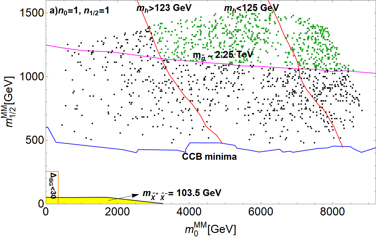
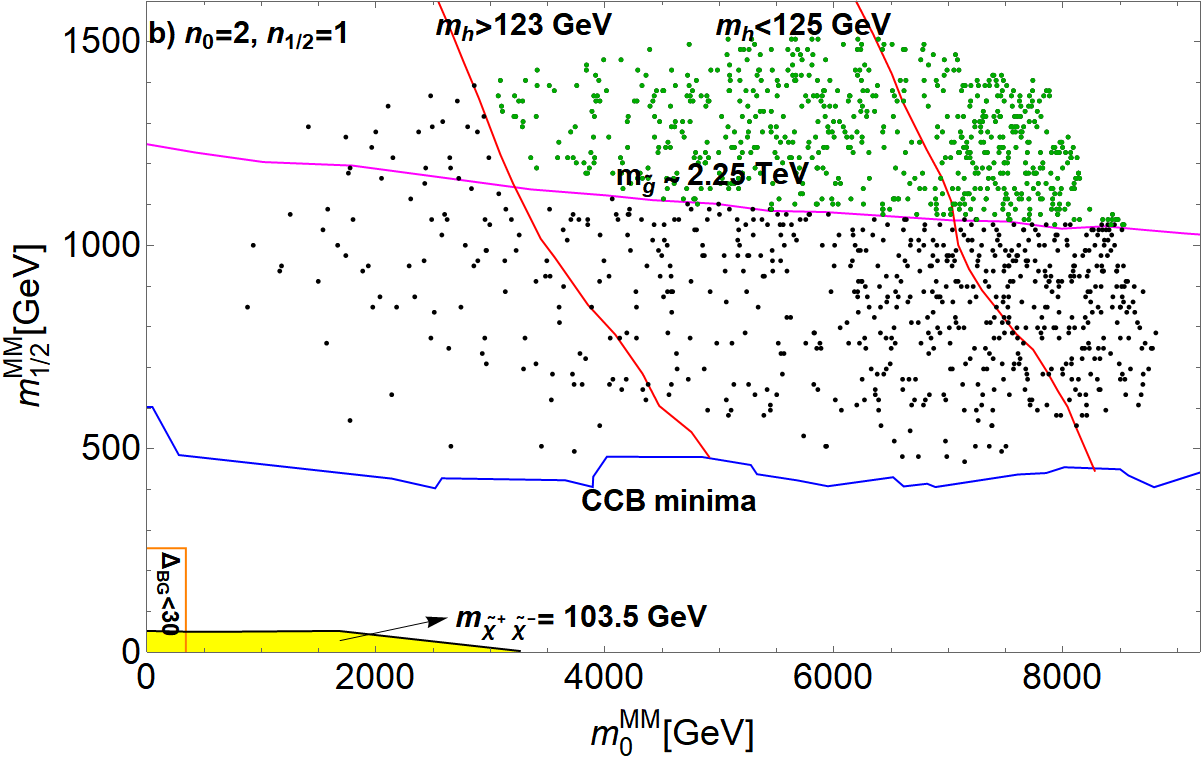
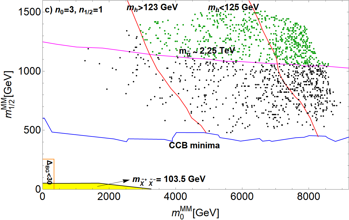
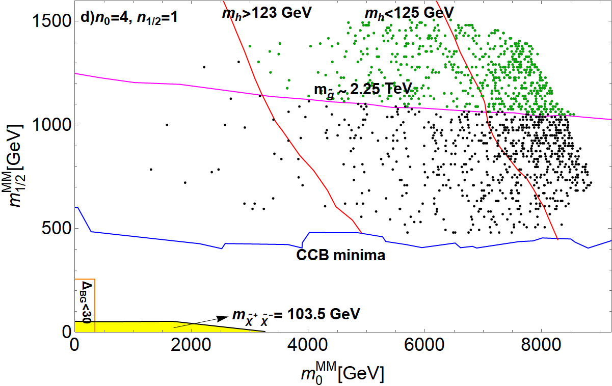
Figure 1: The $m_{0}^{MM}$ vs. $m_{1/2}^{MM}$ plane of the GMM^′ model for a value of $n_{1/2}=1$ for all frames but with a) $n_{0}=1$, b) $n_{0}=2$, c) $n_{0}=3$ and d) $n_{0}=4$. For all frames, we take $m_{3/2}=20$ TeV, $\mu=200$ GeV, $m_{A}=2$ TeV, $\tan\beta=10$ and $a_{3}=1.6\sqrt{c_{m}}$. We require $m_{Z}^{PU}<4m_{Z}^{OU}$.

In Fig. 1a), we show the $m_{0}^{MM}$ vs. $m_{1/2}^{MM}$ plane for the case of an $n_{1/2}=n_{0}=1$ landscape draw but with $a_{3}=1.6\sqrt{c_{m}}$, with $c_{m}=c_{m3}$ and with $\tan\beta=10$, $m_{A}=2$ TeV and $\mu=200$ GeV. The lower-left yellow region shows where $m_{\widetilde{\chi}^{\pm}_{1}}<103.5$ GeV in violation of LEP2 constraints. Also, the lower-left orange box shows where $\Delta_{BG}<30$ (old naturalness calculation). The bulk of the low $m_{1/2}$ region here leads to tachyonic top-squark soft terms owing to the large trilinear terms $A_{0}^{MM}\equiv-a_{3}\alpha(m_{3/2}/16\pi^{2})$. This region is nearly flat with increasing $m_{0}$ mainly because the larger we make the GUT scale top-squark squared mass soft terms, the larger is the cancelling correction from RG running. For larger $m_{1/2}^{MM}$ values, then we obtain viable EW vacua since large values of $M_{3}$ help to enhance top squark squared mass running to large positive values. The dots show the expected statistical result of scanning the landscape, and the larger density of dots on the plot corresponds to greater stringy naturalness. We also show the magenta contour of $m_{\tilde{g}}=2.25$ TeV, below which is excluded by LHC gluino pair searches[79, 80]. We also show contours of $m_{h}=123$ and 125 GeV. The green points are consistent with LHC sparticle search limits and the Higgs mass measurement. From the plot, we see that much of the region of high stringy naturalness tends to lie safely beyond LHC sparticle search limits while at the same time yielding a Higgs mass $m_{h}\simeq 125$ GeV. While early naturalness calculations preferred low $m_{0}$ and $m_{1/2}$ regions[81, 82, 83, 84], we see now that stringy naturalness prefers the opposite[8]: as large as possible values of $m_{0}^{MM}$ and $m_{1/2}^{MM}$ subject to the (anthropic) condition that $m_{weak}^{PU}$ is within a factor four of our measured value (lest the atomic principle be violated). Thus, the most stringy natural region statistically prefers a light Higgs mass $m_{h}\simeq 125$ GeV with sparticles beyond LHC Run 2 reach.

In frame Fig. 1b), we increase the value of $n_{0}$ to 2 while keeping $n_{1/2}$ fixed at 1. Likewise, in frames c) and d), we increase $n_{0}$ to 3 and 4 respectively. The number of dots in the various frames are normalized to $\sim 1500$ so that the relative density, indicating the relative stringy natural regions, can be compared on an equal footing. As $n_{0}$ increases, corresponding to more moduli fields contributing to SUSY breaking in the scalar sector, then the stringy natural region migrates towards higher values of $m_{0}^{MM}$ and a sharpening of the Higgs mass prediction that $m_{h}\simeq 125$ GeV. In fact, in frame d) for $n_{0}=4$, there are only a few scan points with $m_{h}<123$ GeV. An anti-intuitive conclusion from our calculations is that a 3 TeV gluino is more stringy natural than a 300 GeV gluino.

In Fig. 2, we show the histograms of Higgs mass probability for $n_{1/2}=1$ with $n_{0}=1,\ 2,\ 3$ and 4. As seen from the plot, as $n_{0}$ increases, the probability distribution $dP/dm_{h}$ does indeed sharpen around the value of $m_{h}\simeq 125$ GeV.

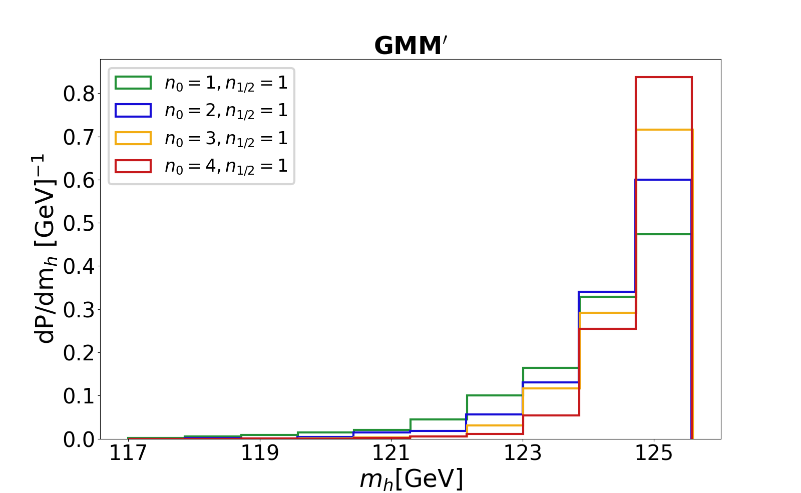
Figure 2: Probability distribution $dP/dm_{h}$ versus $m_{h}$ for $n_{1/2}=1$ and $n_{0}=1,\ 2,\ 3$ and $4$ for scans of the the GMM^′ model for $m_{3/2}=20$ TeV, $\mu=200$ GeV, $m_{A}=2$ TeV, $\tan\beta=10$ and $a_{3}=1.6\sqrt{c_{m}}$. We require $m_{Z}^{PU}<4m_{Z}^{OU}$.

3.3 Parameter space scan procedure for GMM^′ on the landscape

We use Isajet to scan the GMM^′ model parameter space as follows.

• We select a particular value of $m_{3/2}=20$ TeV which then fixes the AMSB contributions to SSB terms.

• We also fix $\mu=200$ GeV for a natural solution to the SUSY $\mu$ problem. This then allows for arbitrary values of $m_{Z}^{PU}$ to be generated but disallows any possibility of fine-tuning $\mu$ to gain the measured value of $m_{Z}^{OU}$ in our universe.

Next, we will invoke Douglas’ power law selection[11, 12, 5] of moduli-mediated soft terms relative to AMSB contributions within the GMM^′ model. Thus, for an assumed value of $n_{1/2}$ and $n_{0}$, we will generate

• $\alpha^{n_{1/2}}$ with $\alpha:3-25$, corresponding to a power law statistical selection for moduli/dilaton-mediated gaugino masses $M_{a}$ $(a=1-3$ over the gauge groups).

• $(a_{3}\alpha)^{n_{0}}$, a power-law statistical selection of moduli-mediated $A$-terms, with $(a_{3}\alpha):3-100$,

• $(\sqrt{c_{m3}\alpha^{2}})^{n_{0}}$ to gain a power-law statistical selection on third generation scalar masses $m_{0}(3)$, with $(\sqrt{c_{m3}\alpha^{2}}):3-80$

• $(\sqrt{c_{m}\alpha^{2}})^{n_{0}}$ to gain a power-law statistical selection on first/second generation scalar masses $m_{0}(1,2)$, with $(\sqrt{c_{m}\alpha^{2}}):\ \sqrt{c_{m3}\alpha^{2}}-320$

• a power-law statistical selection on $m_{H_{d}}^{2}$ via $m_{A}^{n_{0}}$ with $m_{A}:300-10,000$ GeV.

• a uniform selection on $\tan\beta:3-50$.

We adopt a uniform selection on $\tan\beta$ since this parameter is not a soft term. Note that with this procedure– while arbitrarily large soft terms are statistically favored– in fact they are all bounded from above since once they get too big, they will lead either to non-standard EW vacua or else too large a value of $m_{Z}^{PU}$. In this way, models such as split SUSY or high scale SUSY would be ruled out since for a fixed (natural) value of $\mu$ (which is not then available for fine-tuning), they would necessarily lead to $m_{Z}^{PU}\gg(2-5)m_{Z}^{OU}$.

3.4 Higgs and sparticle mass distributions for varying $n_{0}$

In Fig. 3, we show the probability distribution for the light Higgs mass $dP/dm_{h}$ vs. $m_{h}$ from our general landscape scans using $n_{1/2}=1$ but with $n_{0}=1$ (blue) and 2 (red). Both distributions peak around $m_{h}\sim 125$ GeV, but the general scan with the harder $n_{0}=2$ statistical draw on scalar and trilinear soft terms is more sharply peaked around 125 GeV than the $n_{0}=1$ case. This confirms the behavior shown previously in Fig. 2 for the more restrictive scan. We also generated scans with $n_{0}=3$ and 4, but these tend to become very inefficient since as $n_{0}$ increases, one gets pushed almost always into no EWSB or CCB minima, or minima with too large a value of $m_{weak}^{PU}$.

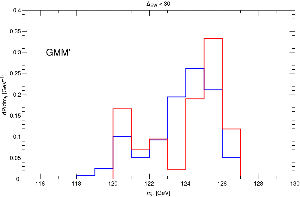
Figure 3: Probability distribution for mass of light Higgs boson $m_{h}$ for $n_{1/2}=1$ with $n_{0}=1$ (blue) and $n_{0}=2$ (red) from statistical scans over the GMM^′ model with $m_{3/2}=20$ TeV.

In Fig. 4, we show probability distributions for a) $dP/dm_{\tilde{g}}$ vs. $m_{\tilde{g}}$, b) $dP/dm_{\tilde{t}_{1}}$ vs. $m_{\tilde{t}_{1}}$, c) $dP/dm_{\tilde{t}_{2}}$ vs. $m_{\tilde{t}_{2}}$ and d) $dP/dm_{A}$ vs. $m_{A}$. From frame a), we see that the landscape prediction for $m_{\tilde{g}}$ lies between 1.5-5 TeV with a peak around 2.5 TeV for $n_{0}=1$ and around 4.5 TeV for $n_{0}=2$. Thus, contrary to traditional naturalness, stringy natural predicts a gluino mass typically well above LHC mass limits. The reach of HE-LHC with $\sqrt{s}=27$ TeV has been computed in Ref. [85] where the 95% CL LHC reach with 15 ab^-1 was found to be $m_{\tilde{g}}\lesssim 6$ TeV. This is to be compared with the ($5\sigma$) reach of HL-LHC with 3 ab^-1 which extends to $m_{\tilde{g}}\sim 2.8$ TeV[86]. Thus, an energy doubling of LHC may well be required to discover SUSY in the $pp\rightarrow\tilde{g}\tilde{g}X$ channel. The distributions for $m_{\tilde{g}}$ change little with varying $n_{0}$ since the gaugino mass distribution depends instead on $n_{1/2}$.

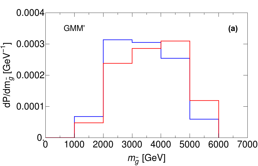
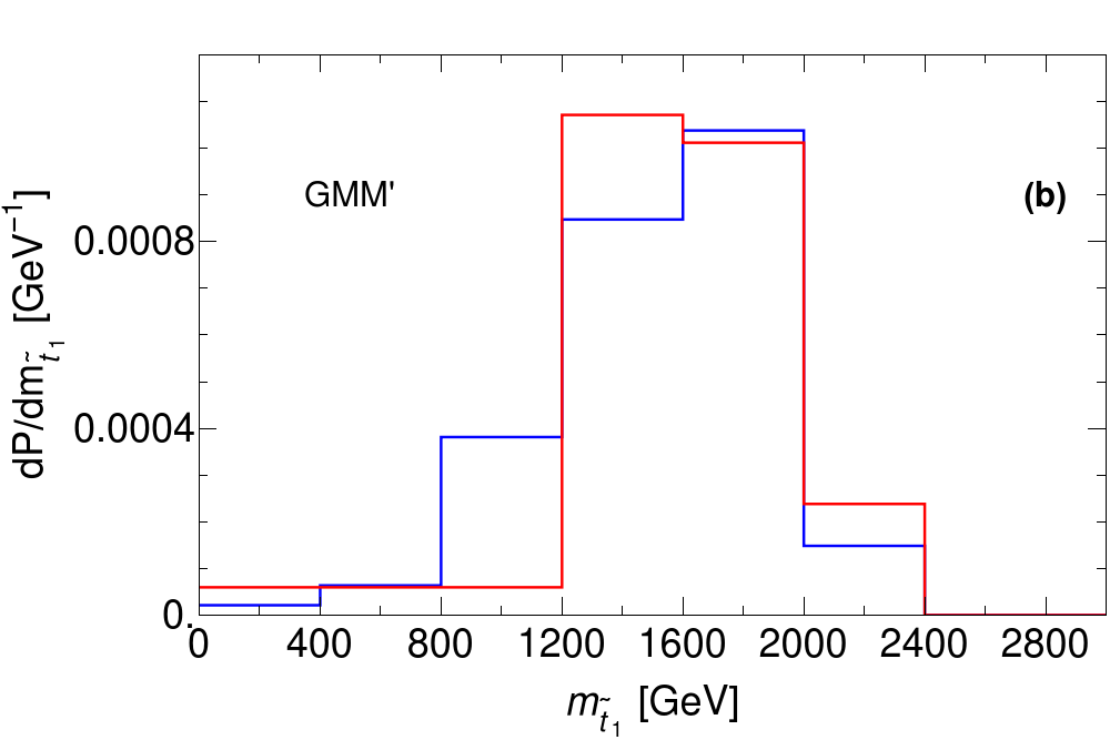
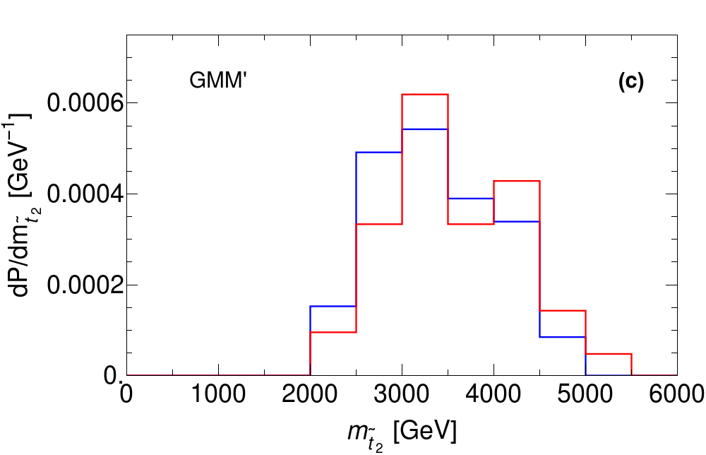
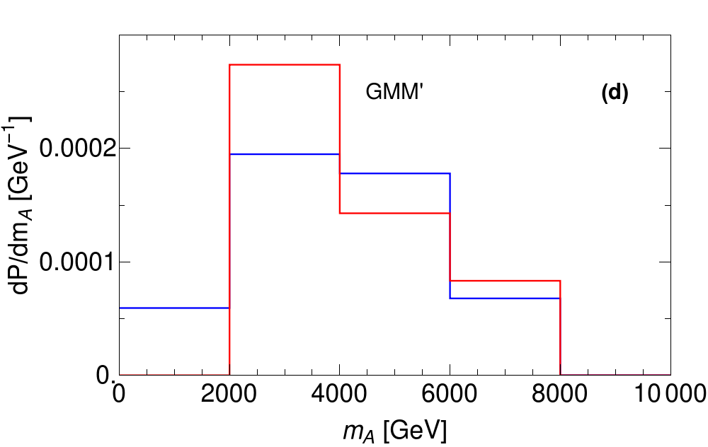
Figure 4: Upper panels: Distributions in $m_{\tilde{g}}$ (left) and $m_{\tilde{t}_{1}}$ (right). Lower panels: Distributions in $m_{\tilde{t}_{2}}$ (left) and $m_{A}$ (right). Here, $n_{1/2}=1$ but $n_{0}=1$ (blue) and $n_{0}=2$ (red) are from statistical scans over the nGMM^′ model with $m_{3/2}=20$ TeV.

In frame b), the landscape probability distribution for $m_{\tilde{t}_{1}}$ lies between $m_{\tilde{t}_{1}}:1-2$ TeV with a peak probability around $m_{\tilde{t}_{1}}\sim 1.5$ TeV for both cases $n_{0}=1$ (blue) and $n_{0}=2$ (red). These distributions hardly depend on the $n_{0}$ value since for fixed $\mu\sim m_{weak}$, then the largest contribution to $m_{weak}$ typically comes from $\Sigma_{u}^{u}(\tilde{t}_{1,2})$ which sets the upper bound on $m_{\tilde{t}_{1}}$. The current limit from LHC Run 2 is that $m_{\tilde{t}_{1}}\gtrsim 1.1$ TeV[87, 88]. Thus, we see that LHC Run 2 has only started exploring the predicted stringy natural parameter space via stop pair production. For comparison, the $5\sigma$ (95% CL) HE-LHC reach with 15 ab^-1 extends to stop masses of 3 (3.5) TeV. Thus, again we would require an approximate doubling of LHC energy in order to cover the entire range of stop masses in landscape SUSY.

In frame c), we see the landscape prediction for $m_{\tilde{t}_{2}}$ lies in the 2-5 TeV range. The reach of HL- and HE-LHC for $\tilde{t}_{2}$ should be similar to their reaches for $m_{\tilde{t}_{1}}$. Thus, we would expect HE-LHC to cover only about half the expected mass range for the heavier top-squark $\tilde{t}_{2}$. The predicted statistical distribution for $m_{\tilde{t}_{2}}$ shifts to higher $m_{\tilde{t}_{2}}$ values for larger $n_{0}$ as might be expected.

In frame d), we find the distribution for $m_{A}$ to lie within the $m_{A}\sim 1-8$ TeV range with a peak around $m_{A}\sim 3$ TeV for both $n_{0}=1$ and $n_{0}=2$. The upper bound on $m_{A}$ comes from the $m_{H_{d}}^{2}/(\tan^{2}\beta-1)$ term in Eq. 2: if it is too large, then $m_{weak}^{PU}$ will become too large. From this point of view, it is not surprising that the Higgs sector looks highly SM-like at LHC so far since there is a decoupling of heavier Higgs particles embedded mainly in the $H_{d}$ multiplet while the $H_{u}$ multiplet is very SM-like.

In Fig. 5, we show the string landscape prediction for first/second generation matter scalars, as typified by $m_{\tilde{u}_{L}}$. From this plot, for $n_{1/2}=1$ and $n_{0}=1$, then we see that first/second generation matter scalars extend from 10-35 TeV with a peak distribution around $m_{\tilde{u}_{L}}\sim 22$ TeV. The upper bound on first/second generation matter scalars arises not from Yukawa terms (tiny) or $D$-terms (which largely cancel) but from 2-loop RGE contributions which, if they get too large– can drive top-squark soft terms to tachyonic values. As we increase $n_{0}$ to 2, then the distribution in $m_{\tilde{u}_{L}}$ hardens even further to a peak around $m_{\tilde{u}_{L}}\sim 30$ TeV. Both first and second generation matter scalars are pulled to a common upper bound since the two-loop RGE terms are flavor independent. This leads to the string landscape mixed quasi-degeneracy/decoupling solution to the SUSY flavor and CP problems[16]. In fact, in previous times model builders fought a hard battle to find schemes which lead to universal scalar masses as a means to solve the SUSY flavor problem. In contrast, in the string landscape picture, the expected non-universality of scalar masses turns out to be an asset since the different soft terms can be drawn to sufficiently large values while their contributions to the weak scale remain small. This mechanism leads to its own mixed quasi-degeneracy/decoupling solution to the SUSY flavor and CP problems.

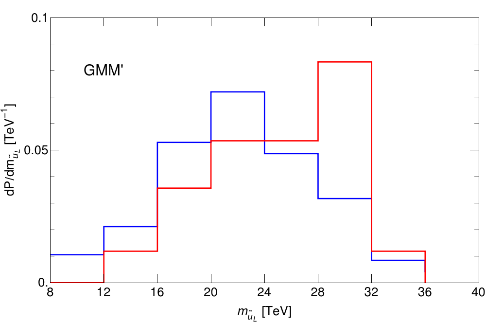
Figure 5: Probability distribution $dP/dm_{\tilde{u}_{L}}$ vs. $m_{\tilde{u}_{L}}$ from general scan for $n_{1/2}=1$ but for $n_{0}=1$ and 2.

4 Conclusions

In this paper, our main goal was to examine the form of soft SUSY breaking terms that would arise in string compactifications to a $4-d$, $N=1$ supergravity theory including the MSSM as the low energy EFT. We assumed the EFT consisted of the usual MSSM visible sector fields along with a hidden sector of moduli fields which would serve as the arena for SUSY breaking. Using the well-known formulae for soft SUSY breaking terms in $N=1$ SUGRA, then we would expect the gaugino masses $m_{1/2}$, the various scalar masses $m_{0}(i)$, $m_{H_{u,d}}$ and the $A$-terms to scan independently due to their different functional dependence on the moduli fields.

For the soft breaking scalar masses, we expect generally non-universal soft terms due to different dependence of the Kähler metric on the compactified space. This reflects the expected geography of visible sector fields on the compactified manifold, as emphasized by Nilles and Vaudrevange[90], whose conclusions were drawn from the context of heterotic orbifold models. In past times, non-universality of soft scalar masses was a thing to be avoided in that it could lead to dangerous flavor-violating processes. Various contorted model-building efforts were thus made to avoid the generic non-universality expected from realistic string compactifications. However, in the context of the string landscape, scalar mass non-universality turns out to be a desired property. This is because the landscape likely contains a statistical draw towards large soft terms, especially in the scalar mass sector. The draw to large $m_{H_{u}}^{2}$, which stops just short of the living dangerously feature of “no-EWSB”, pulls $m_{H_{u}}^{2}$ to values associated with radiatively-driven naturalness, wherein large high scale soft terms are evolved via RGEs to natural values at the weak scale. Likewise, $A$-terms are drawn large enough to generate maximal mixing in the stop sector, thus minimizing the top-squark contributions to the weak scale whilst lifting $m_{h}\rightarrow 125$ GeV, while stopping short of such large values as to generate CCB minima in the scalar potential. Also, first/second generation scalars are drawn to a common upper bound in the 20-40 TeV range which leads to a mixed quasi-degeneracy/decoupling solution to the SUSY flavor and CP problems.

We also examined the soft terms in the context of how strongly they would be statistically drawn to large values by the string landscape. In many viable string models, the tree level gauge kinetic function depends only on the dilaton field so that a statistical pull of $m(gaugino)^{n_{1/2}}$ with $n_{1/2}=1$ is expected. In contrast, the scalar masses and $A$-terms typically depend on all the moduli fields which would contribute to SUSY breaking, and thus a much stronger draw of $m_{soft}^{n_{0}}$ with $n_{0}\gg 1$ may be expected.

We illustrated the consequences of these different statistical draws in our scans over generalized mirage-mediation model GMM^′ parameter space wherein comparable moduli-mediated and anomaly-mediated contributions to soft terms arise. The cases with $n_{0}>n_{1/2}$ lead to predictions of greater splitting in the SUSY particle mass spectrum with first/second generation scalar masses $\gg$ third generation and gaugino masses. As $n_{0}$ increases relative to $n_{1/2}$, the Higgs mass probability distribution sharpens even more to its expected peak at $m_{h}\sim 125$ GeV.

What are the phenomenological consequences of the string landscape for LHC and dark matter searches? Our results are summarized in Table 1 from our scans over the GMM^′ model with $n_{1/2}=1$ and with $n_{0}=1$ or 2. Typically, our statistical landscape approch to SUSY phenomenology predicts a Higgs mass $m_{h}\simeq 125$ GeV with sparticle masses beyond LHC reach. Since the landscape predicts $m_{\tilde{g}}\sim 3.5\pm 2.5$ TeV and $m_{\tilde{t}_{1}}\sim 1.6\pm 0.8$ TeV, then an energy upgrade of LHC to at least $\sqrt{s}\sim 27$ TeV may be needed for SUSY discovery in the gluino pair or top-squark pair production channels. However, since the higgsino mass parameter $\mu$ is required not-to-far from $m_{weak}\sim 100$ GeV, it might be possible for LHC experiments to eke out a signal from direct higgsino pair production reactions such as $pp\rightarrow\widetilde{\chi}^{0}_{1}\widetilde{\chi}^{0}_{2}$ in the soft, opposite-sign dilepton channel[20], perhaps in association with a hard jet radiation[91, 92, 93, 94]. The parameter space for this SUSY discovery channel is just beginning to be explored[95].

mass	$n_{0}=1$	$n_{0}=2$
$m_{h}$	$125^{+1}_{-4}$ GeV	$125^{+1}_{-4}$ GeV
$m_{\tilde{g}}$	$3.5\pm 2.5$ TeV	$4\pm 2$ TeV
$m_{\tilde{t}_{1}}$	$1.6\pm 0.8$ TeV	$1.6\pm 0.8$ TeV
$m_{\tilde{t}_{2}}$	$3.5\pm 1.5$ TeV	$3.5\pm 1.5$ TeV
$m_{A}$	$4\pm 2$ TeV	$4\pm 2$ TeV
$m_{\tilde{f}}(1,2)$	$22\pm 10$ TeV	$30^{+6}_{-18}$ TeV

Table 1: Expected range of Higgs and sparticle masses in the generalized mirage mediation (GMM^′) model from the string landscape with $n_{1/2}=1$ but with $n_{0}=1$ or $n_{0}=2$.

Regarding dark matter, we would expect it to be composed of both SUSY DFSZ axions[96, 56] (which have a suppressed coupling to photons[97]) along with a smaller component ($\sim 10-20$%) of higgsino-like WIMPs[98]. The multi-ton noble liquid detectors now being deployed should have future sensitivity to the entire expected parameter space[99], so we would expect a WIMP discovery should still be forthcoming in the next 5-10 years.

Acknowledgements:

This material is based upon work supported by the U.S. Department of Energy, Office of Science, Office of High Energy Physics under Award Number DE-SC-0009956.

References

References

-
[1]
S. Weinberg,
Anthropic bound
on the cosmological constant, Phys. Rev. Lett. 59 (1987) 2607–2610.
doi:10.1103/PhysRevLett.59.2607.
URL https://link.aps.org/doi/10.1103/PhysRevLett.59.2607 -
[2]
S. Weinberg, The
cosmological constant problem, Rev. Mod. Phys. 61 (1989) 1–23.
doi:10.1103/RevModPhys.61.1.
URL https://link.aps.org/doi/10.1103/RevModPhys.61.1 -
[3]
L. Susskind, The Anthropic
landscape of string theory (2003) 247–266arXiv:hep-th/0302219.
URL https://arxiv.org/abs/hep-th/0302219 -
[4]
F. Denef, M. R. Douglas,
Distributions of flux
vacua, Journal of High Energy Physics 2004 (05) (2004) 072–072.
doi:10.1088/1126-6708/2004/05/072.
URL http://dx.doi.org/10.1088/1126-6708/2004/05/072 - [5] N. Arkani-Hamed, S. Dimopoulos, S. Kachru, Predictive landscapes and new physics at a TeVarXiv:hep-th/0501082.
-
[6]
M. K. Gaillard, B. W. Lee,
Rare decay modes of
the k mesons in gauge theories, Phys. Rev. D 10 (1974) 897–916.
doi:10.1103/PhysRevD.10.897.
URL https://link.aps.org/doi/10.1103/PhysRevD.10.897 -
[7]
M. R. Douglas, Basic
results in vacuum statistics, Comptes Rendus Physique 5 (9-10) (2004)
965–977.
doi:10.1016/j.crhy.2004.09.008.
URL http://dx.doi.org/10.1016/j.crhy.2004.09.008 -
[8]
H. Baer, V. Barger, S. Salam,
Naturalness
versus stringy naturalness with implications for collider and dark matter
searches, Phys. Rev. Research 1 (2019) 023001.
doi:10.1103/PhysRevResearch.1.023001.
URL https://link.aps.org/doi/10.1103/PhysRevResearch.1.023001 - [9] K. J. Bae, H. Baer, V. Barger, D. Sengupta, Revisiting the susy mu problem and its solutions in the lhc era, Physical Review D 99 (11). doi:10.1103/PhysRevD.99.115027.
-
[10]
H. Baer, V. Barger, P. Huang, D. Mickelson, A. Mustafayev, X. Tata,
Radiative natural
supersymmetry: Reconciling electroweak fine-tuning and the higgs boson mass,
Phys. Rev. D 87 (2013) 115028.
doi:10.1103/PhysRevD.87.115028.
URL https://link.aps.org/doi/10.1103/PhysRevD.87.115028 - [11] M. R. Douglas, Statistical analysis of the supersymmetry breaking scalearXiv:hep-th/0405279.
- [12] L. Susskind, Supersymmetry breaking in the anthropic landscape (2004) 1745–1749arXiv:hep-th/0405189, doi:10.1142/9789812775344\_0040.
-
[13]
H. Baer, V. Barger, H. Serce, K. Sinha,
Higgs and superparticle mass
predictions from the landscape, Journal of High Energy Physics 2018 (3).
doi:10.1007/jhep03(2018)002.
URL http://dx.doi.org/10.1007/JHEP03(2018)002 -
[14]
H. Baer, V. Barger, M. Savoy, H. Serce,
The higgs mass and
natural supersymmetric spectrum from the landscape, Physics Letters B 758
(2016) 113–117.
doi:10.1016/j.physletb.2016.05.010.
URL http://dx.doi.org/10.1016/j.physletb.2016.05.010 -
[15]
H. Baer, V. Barger, P. Huang, A. Mustafayev, X. Tata,
Radiative natural
supersymmetry with a 125 gev higgs boson, Physical Review Letters 109 (16).
doi:10.1103/physrevlett.109.161802.
URL http://dx.doi.org/10.1103/PhysRevLett.109.161802 -
[16]
H. Baer, V. Barger, D. Sengupta,
Landscape solution
to the susy flavor and cp problems, Physical Review Research 1 (3).
doi:10.1103/physrevresearch.1.033179.
URL http://dx.doi.org/10.1103/PhysRevResearch.1.033179 -
[17]
V. Agrawal, S. M. Barr, J. F. Donoghue, D. Seckel,
Viable range of the mass
scale of the standard model, Physical Review D 57 (9) (1998) 5480–5492.
doi:10.1103/physrevd.57.5480.
URL http://dx.doi.org/10.1103/PhysRevD.57.5480 -
[18]
V. Agrawal, S. M. Barr, J. F. Donoghue, D. Seckel,
Anthropic
considerations in multiple-domain theories and the scale of electroweak
symmetry breaking, Phys. Rev. Lett. 80 (1998) 1822–1825.
doi:10.1103/PhysRevLett.80.1822.
URL https://link.aps.org/doi/10.1103/PhysRevLett.80.1822 -
[19]
H. Baer, V. Barger, D. Sengupta,
Mirage mediation
from the landscape, Physical Review Research 2 (1).
doi:10.1103/physrevresearch.2.013346.
URL http://dx.doi.org/10.1103/PhysRevResearch.2.013346 -
[20]
H. Baer, V. Barger, P. Huang,
Hidden susy at the lhc: the
light higgsino-world scenario and the role of a lepton collider, Journal of
High Energy Physics 2011 (11).
doi:10.1007/jhep11(2011)031.
URL http://dx.doi.org/10.1007/JHEP11(2011)031 -
[21]
H. Baer, V. Barger, H. Serce, X. Tata,
Natural generalized
mirage mediation, Physical Review D 94 (11).
doi:10.1103/physrevd.94.115017.
URL http://dx.doi.org/10.1103/PhysRevD.94.115017 -
[22]
V. S. Kaplunovsky, J. Louis,
Model-independent
analysis of soft terms in effective supergravity and in string theory,
Physics Letters B 306 (3-4) (1993) 269–275.
doi:10.1016/0370-2693(93)90078-v.
URL http://dx.doi.org/10.1016/0370-2693(93)90078-V -
[23]
A. Brignole, Towards a
theory of soft terms for the supersymmetric standard model, Nuclear Physics
B 422 (1-2) (1994) 125–171.
doi:10.1016/0550-3213(94)00068-9.
URL http://dx.doi.org/10.1016/0550-3213(94)00068-9 -
[24]
S. Kachru, R. Kallosh, A. Linde, S. P. Trivedi,
de sitter vacua in string
theory, Physical Review D 68 (4).
doi:10.1103/physrevd.68.046005.
URL http://dx.doi.org/10.1103/PhysRevD.68.046005 -
[25]
V. Balasubramanian, P. Berglund, J. P. Conlon, F. Quevedo,
Systematics of moduli
stabilisation in calabi-yau flux compactifications, Journal of High Energy
Physics 2005 (03) (2005) 007–007.
doi:10.1088/1126-6708/2005/03/007.
URL http://dx.doi.org/10.1088/1126-6708/2005/03/007 - [26] S. K. Soni, H. Weldon, Analysis of the Supersymmetry Breaking Induced by N=1 Supergravity Theories, Phys. Lett. B 126 (1983) 215–219. doi:10.1016/0370-2693(83)90593-2.
- [27] E. Cremmer, S. Ferrara, L. Girardello, A. Van Proeyen, Yang-Mills Theories with Local Supersymmetry: Lagrangian, Transformation Laws and SuperHiggs Effect, Nucl. Phys. B 212 (1983) 413. doi:10.1016/0550-3213(83)90679-X.
-
[28]
K. Choi, A. Falkowski, H. Nilles, M. Olechowski,
Soft supersymmetry
breaking in kklt flux compactification, Nuclear Physics B 718 (1-2) (2005)
113–133.
doi:10.1016/j.nuclphysb.2005.04.032.
URL http://dx.doi.org/10.1016/j.nuclphysb.2005.04.032 - [29] K. R. Dienes, C. F. Kolda, Twenty open questions in supersymmetric particle physicsarXiv:hep-ph/9712322.
-
[30]
O. Lebedev, H. P. Nilles, S. Raby, S. Ramos-Sánchez, M. Ratz, P. K.
Vaudrevange, A. Wingerter,
A mini-landscape of
exact mssm spectra in heterotic orbifolds, Physics Letters B 645 (1) (2007)
88–94.
doi:10.1016/j.physletb.2006.12.012.
URL http://dx.doi.org/10.1016/j.physletb.2006.12.012 - [31] W. Buchmuller, K. Hamaguchi, O. Lebedev, M. Ratz, Local grand unification, in: GUSTAVOFEST: Symposium in Honor of Gustavo C. Branco: CP Violation and the Flavor Puzzle, 2005, pp. 143–156. arXiv:hep-ph/0512326.
- [32] M. Ratz, Notes on Local Grand Unification, Soryushiron Kenkyu Electron. 116 (2008) A56–A76. arXiv:0711.1582, doi:10.24532/soken.116.1\_A56.
- [33] L. Ibanez, G. G. Ross, Su (2) l u (1) symmetry breaking as a radiative effect of supersymmetry breaking in guts, Physics Letters B 110 (3-4) (1982) 215–220.
-
[34]
K. Inoue, A. Kakuto, H. Komatsu, S. Takeshita,
Aspects of Grand Unified Models
with Softly Broken Supersymmetry, Progress of Theoretical Physics 68 (3)
(1982) 927–946.
arXiv:https://academic.oup.com/ptp/article-pdf/68/3/927/5420860/68-3-927.pdf,
doi:10.1143/PTP.68.927.
URL https://doi.org/10.1143/PTP.68.927 -
[35]
K. Inoue, A. Kakuto, H. Komatsu, S. Takeshita,
Renormalization of Supersymmetry
Breaking Parameters Revisited, Progress of Theoretical Physics 71 (2)
(1984) 413–416.
arXiv:https://academic.oup.com/ptp/article-pdf/71/2/413/5460589/71-2-413.pdf,
doi:10.1143/PTP.71.413.
URL https://doi.org/10.1143/PTP.71.413 - [36] L. E. Ibanez, Locally supersymmetric su (5) grand unification, Phys. Lett. B 118 (CERN-TH-3374) (1982) 73–78.
- [37] H. P. Nilles, M. Srednicki, D. Wyler, Weak Interaction Breakdown Induced by Supergravity, Phys. Lett. B 120 (1983) 346. doi:10.1016/0370-2693(83)90460-4.
-
[38]
J. Ellis, J. S. Hagelin, D. Nanopoulos, K. Tamvakis,
Observable
gravitationally induced baryon decay, Physics Letters B 124 (6) (1983) 484
– 490.
doi:https://doi.org/10.1016/0370-2693(83)91557-5.
URL http://www.sciencedirect.com/science/article/pii/0370269383915575 - [39] L. Alvarez-Gaume, J. Polchinski, M. B. Wise, Minimal low-energy supergravity, Nuclear Physics B 221 (2) (1983) 495–523.
-
[40]
M. Dine, A. E. Nelson, Y. Nir, Y. Shirman,
New tools for low energy
dynamical supersymmetry breaking, Physical Review D 53 (5) (1996)
2658–2669.
doi:10.1103/physrevd.53.2658.
URL http://dx.doi.org/10.1103/PhysRevD.53.2658 -
[41]
G. Giudice, R. Rattazzi,
Theories with
gauge-mediated supersymmetry breaking, Physics Reports 322 (6) (1999)
419–499.
doi:10.1016/s0370-1573(99)00042-3.
URL http://dx.doi.org/10.1016/S0370-1573(99)00042-3 -
[42]
L. Randall, R. Sundrum,
Out of this world
supersymmetry breaking, Nuclear Physics B 557 (1-2) (1999) 79–118.
doi:10.1016/s0550-3213(99)00359-4.
URL http://dx.doi.org/10.1016/S0550-3213(99)00359-4 -
[43]
G. F. Giudice, R. Rattazzi, M. A. Luty, H. Murayama,
Gaugino mass without
singlets, Journal of High Energy Physics 1998 (12) (1998) 027–027.
doi:10.1088/1126-6708/1998/12/027.
URL http://dx.doi.org/10.1088/1126-6708/1998/12/027 -
[44]
J. A. Bagger, T. Moroi, E. Poppitz,
Anomaly mediation in
supergravity theories, Journal of High Energy Physics 2000 (04) (2000)
009–009.
doi:10.1088/1126-6708/2000/04/009.
URL http://dx.doi.org/10.1088/1126-6708/2000/04/009 -
[45]
P. Binétruy, M. K. Gaillard, B. D. Nelson,
One loop soft
supersymmetry breaking terms in superstring effective theories, Nuclear
Physics B 604 (1-2) (2001) 32–74.
doi:10.1016/s0550-3213(00)00759-8.
URL http://dx.doi.org/10.1016/S0550-3213(00)00759-8 -
[46]
H. Baer, V. Barger, D. Sengupta,
Anomaly-mediated susy
breaking model retrofitted for naturalness, Physical Review D 98 (1).
doi:10.1103/physrevd.98.015039.
URL http://dx.doi.org/10.1103/PhysRevD.98.015039 -
[47]
A. Arbey, M. Battaglia, A. Djouadi, F. Mahmoudi, J. Quevillon,
Implications of a 125
gev higgs for supersymmetric models, Physics Letters B 708 (1-2) (2012)
162–169.
doi:10.1016/j.physletb.2012.01.053.
URL http://dx.doi.org/10.1016/j.physletb.2012.01.053 -
[48]
P. Draper, P. Meade, M. Reece, D. Shih,
Implications of a
125 gev higgs boson for the mssm and low-scale supersymmetry breaking,
Physical Review D 85 (9).
doi:10.1103/physrevd.85.095007.
URL http://dx.doi.org/10.1103/PhysRevD.85.095007 -
[49]
H. Baer, V. Barger, A. Mustafayev,
Neutralino dark matter in
msugra/ with a 125 gev light higgs scalar, Journal of High Energy Physics
2012 (5).
doi:10.1007/jhep05(2012)091.
URL http://dx.doi.org/10.1007/JHEP05(2012)091 -
[50]
H. Baer, V. Barger, S. Salam,
Naturalness versus
stringy naturalness (with implications for collider and dark matter
searches), Physical Review Research 1 (2).
doi:10.1103/physrevresearch.1.023001.
URL http://dx.doi.org/10.1103/PhysRevResearch.1.023001 - [51] J. Casas, C. Munoz, A Natural solution to the mu problem, Phys. Lett. B 306 (1993) 288–294. arXiv:hep-ph/9302227, doi:10.1016/0370-2693(93)90081-R.
- [52] G. Giudice, A. Masiero, A Natural Solution to the mu Problem in Supergravity Theories, Phys. Lett. B 206 (1988) 480–484. doi:10.1016/0370-2693(88)91613-9.
-
[53]
U. Ellwanger, C. Hugonie, A. M. Teixeira,
The next-to-minimal
supersymmetric standard model, Physics Reports 496 (1-2) (2010) 1–77.
doi:10.1016/j.physrep.2010.07.001.
URL http://dx.doi.org/10.1016/j.physrep.2010.07.001 -
[54]
K. J. Bae, E. J. Chun, S. H. Im,
Cosmology of the
dfsz2 axino, Journal of Cosmology and Astroparticle Physics 2012 (03)
(2012) 013–013.
doi:10.1088/1475-7516/2012/03/013.
URL https://doi.org/10.1088%2F1475-7516%2F2012%2F03%2F013 - [55] K. J. Bae, H. Baer, E. J. Chun, Mixed axion/neutralino dark matter in the SUSY dfsz2 axion model, JCAP 12 (2013) 028. arXiv:1309.5365, doi:10.1088/1475-7516/2013/12/028.
-
[56]
K. J. Bae, H. Baer, E. J. Chun,
Mixed axion/neutralino
dark matter in the susy dfsz axion model, Journal of Cosmology and
Astroparticle Physics 2013 (12) (2013) 028–028.
doi:10.1088/1475-7516/2013/12/028.
URL http://dx.doi.org/10.1088/1475-7516/2013/12/028 -
[57]
M. Dine, W. Fischler, M. Srednicki,
A
simple solution to the strong cp problem with a harmless axion, Physics
Letters B 104 (3) (1981) 199 – 202.
doi:https://doi.org/10.1016/0370-2693(81)90590-6.
URL http://www.sciencedirect.com/science/article/pii/0370269381905906 - [58] A. Zhitnitsky, On Possible Suppression of the Axion Hadron Interactions. (In Russian), Sov. J. Nucl. Phys. 31 (1980) 260.
-
[59]
S. M. Barr, D. Seckel,
Planck-scale
corrections to axion models, Phys. Rev. D 46 (1992) 539–549.
doi:10.1103/PhysRevD.46.539.
URL https://link.aps.org/doi/10.1103/PhysRevD.46.539 -
[60]
R. Holman, S. D. Hsu, T. W. Kephart, E. W. Kolb, R. Watkins, L. M. Widrow,
Solutions to the
strong-cp problem in a world with gravity, Physics Letters B 282 (1-2)
(1992) 132–136.
doi:10.1016/0370-2693(92)90491-l.
URL http://dx.doi.org/10.1016/0370-2693(92)90491-L - [61] M. Kamionkowski, J. March-Russell, Planck scale physics and the Peccei-Quinn mechanism, Phys. Lett. B 282 (1992) 137–141. arXiv:hep-th/9202003, doi:10.1016/0370-2693(92)90492-M.
-
[62]
R. Kallosh, A. Linde, D. Linde, L. Susskind,
Gravity and global
symmetries, Physical Review D 52 (2) (1995) 912–935.
doi:10.1103/physrevd.52.912.
URL http://dx.doi.org/10.1103/PhysRevD.52.912 -
[63]
K. Babu, I. Gogoladze, K. Wang,
Stabilizing the axion
by discrete gauge symmetries, Physics Letters B 560 (3-4) (2003) 214–222.
doi:10.1016/s0370-2693(03)00411-8.
URL http://dx.doi.org/10.1016/S0370-2693(03)00411-8 -
[64]
H. M. Lee, S. Raby, M. Ratz, G. G. Ross, R. Schieren, K. Schmidt-Hoberg, P. K.
Vaudrevange,
Discrete r
symmetries for the mssm and its singlet extensions, Nuclear Physics B
850 (1) (2011) 1–30.
doi:10.1016/j.nuclphysb.2011.04.009.
URL http://dx.doi.org/10.1016/j.nuclphysb.2011.04.009 -
[65]
H. Baer, V. Barger, D. Sengupta,
Gravity safe,
electroweak natural axionic solution to strong cp and susy mu problems,
Physics Letters B 790 (2019) 58–63.
doi:10.1016/j.physletb.2019.01.007.
URL http://dx.doi.org/10.1016/j.physletb.2019.01.007 -
[66]
H. Baer, V. Barger, D. Mickelson, A. Mustafayev, X. Tata,
Physics at a higgsino
factory, Journal of High Energy Physics 2014 (6).
doi:10.1007/jhep06(2014)172.
URL http://dx.doi.org/10.1007/JHEP06(2014)172 - [67] H. Baer, M. Berggren, K. Fujii, J. List, S.-L. Lehtinen, T. Tanabe, J. Yan, The ILC as a natural SUSY discovery machine and precision microscope: from light higgsinos to tests of unification, Phys. Rev. D 101 (9) (2020) 095026. arXiv:1912.06643, doi:10.1103/PhysRevD.101.095026.
-
[68]
K. Choi, K.-S. Jeong, K.-i. Okumura,
Phenomenology of mixed
modulus-anomaly mediation in fluxed string compactifications and brane
models, Journal of High Energy Physics 2005 (09) (2005) 039–039.
doi:10.1088/1126-6708/2005/09/039.
URL http://dx.doi.org/10.1088/1126-6708/2005/09/039 -
[69]
A. Falkowski, O. Lebedev, Y. Mambrini,
Susy phenomenology of
kklt flux compactifications, Journal of High Energy Physics 2005 (11) (2005)
034–034.
doi:10.1088/1126-6708/2005/11/034.
URL http://dx.doi.org/10.1088/1126-6708/2005/11/034 -
[70]
K. Choi, K. S. Jeong, T. Kobayashi, K.-i. Okumura,
Tev scale mirage
mediation and natural little supersymmetric hierarchy, Phys. Rev. D 75
(2007) 095012.
doi:10.1103/PhysRevD.75.095012.
URL https://link.aps.org/doi/10.1103/PhysRevD.75.095012 - [71] M. Endo, M. Yamaguchi, K. Yoshioka, A Bottom-up approach to moduli dynamics in heavy gravitino scenario: Superpotential, soft terms and sparticle mass spectrum, Phys. Rev. D 72 (2005) 015004. arXiv:hep-ph/0504036, doi:10.1103/PhysRevD.72.015004.
-
[72]
D. Matalliotakis, H. Nilles,
Implications of
non-universality of soft terms in supersyrnmetric grand unified theories,
Nuclear Physics B 435 (1-2) (1995) 115–128.
doi:10.1016/0550-3213(94)00487-y.
URL http://dx.doi.org/10.1016/0550-3213(94)00487-Y -
[73]
M. Olechowski, S. Pokorski,
Electroweak symmetry
breaking with non-universal scalar soft terms and large tan β solutions,
Physics Letters B 344 (1-4) (1995) 201–210.
doi:10.1016/0370-2693(94)01571-s.
URL http://dx.doi.org/10.1016/0370-2693(94)01571-S -
[74]
P. Nath, R. Arnowitt,
Non-universal soft susy
breaking and dark matter, COSMO-97doi:10.1142/9789814447263_0020.
URL http://dx.doi.org/10.1142/9789814447263_0020 -
[75]
J. Ellis, K. Olive, Y. Santoso,
The mssm parameter
space with non-universal higgs masses, Physics Letters B 539 (1-2) (2002)
107–118.
doi:10.1016/s0370-2693(02)02071-3.
URL http://dx.doi.org/10.1016/S0370-2693(02)02071-3 -
[76]
J. Ellis, T. Falk, K. A. Olive, Y. Santoso,
Exploration of the
mssm with non-universal higgs masses, Nuclear Physics B 652 (2003)
259–347.
doi:10.1016/s0550-3213(02)01144-6.
URL http://dx.doi.org/10.1016/S0550-3213(02)01144-6 - [77] H. Baer, A. Mustafayev, S. Profumo, A. Belyaev, X. Tata, Direct, indirect and collider detection of neutralino dark matter in SUSY models with non-universal Higgs masses, JHEP 07 (2005) 065. arXiv:hep-ph/0504001, doi:10.1088/1126-6708/2005/07/065.
- [78] F. E. Paige, S. D. Protopopescu, H. Baer, X. Tata, ISAJET 7.69: A Monte Carlo event generator for pp, anti-p p, and e+e- reactionsarXiv:hep-ph/0312045.
- [79] K. Uno, Search for squarks and gluinos in final states with jets and missing transverse momentum at = 13 TeV using 139 fb-1 data with the ATLAS detector, PoS LeptonPhoton2019 (2019) 186. doi:10.22323/1.367.0186.
-
[80]
A. M. Sirunyan, A. Tumasyan, W. Adam, F. Ambrogi, T. Bergauer, J. Brandstetter,
M. Dragicevic, J. Erö, A. Escalante Del Valle, et al.,
Search for supersymmetry in
proton-proton collisions at 13 tev in final states with jets and missing
transverse momentum, Journal of High Energy Physics 2019 (10).
doi:10.1007/jhep10(2019)244.
URL http://dx.doi.org/10.1007/JHEP10(2019)244 - [81] J. R. Ellis, K. Enqvist, D. V. Nanopoulos, F. Zwirner, Observables in Low-Energy Superstring Models, Mod. Phys. Lett. A 1 (1986) 57. doi:10.1142/S0217732386000105.
-
[82]
R. Barbieri, G. F. Giudice, Upper
bounds on supersymmetric particle masses, Nucl. Phys. B
306 (CERN-TH-4825-87) (1987) 63–76. 19 p.
doi:10.1016/0550-3213(88)90171-X.
URL https://cds.cern.ch/record/180560 -
[83]
S. Dimopoulos, G. Giudice,
Naturalness constraints
in supersymmetric theories with non-universal soft terms, Physics Letters B
357 (4) (1995) 573–578.
doi:10.1016/0370-2693(95)00961-j.
URL http://dx.doi.org/10.1016/0370-2693(95)00961-J -
[84]
G. W. Anderson, D. J. Castaño,
Challenging
weak-scale supersymmetry at colliders, Phys. Rev. D 53 (1996) 2403–2410.
doi:10.1103/PhysRevD.53.2403.
URL https://link.aps.org/doi/10.1103/PhysRevD.53.2403 -
[85]
H. Baer, V. Barger, J. S. Gainer, D. Sengupta, H. Serce, X. Tata,
Lhc luminosity and energy
upgrades confront natural supersymmetry models, Physical Review D 98 (7).
doi:10.1103/physrevd.98.075010.
URL http://dx.doi.org/10.1103/PhysRevD.98.075010 -
[86]
H. Baer, V. Barger, J. S. Gainer, P. Huang, M. Savoy, D. Sengupta, X. Tata,
Gluino reach and mass
extraction at the lhc in radiatively-driven natural susy, The European
Physical Journal C 77 (7).
doi:10.1140/epjc/s10052-017-5067-3.
URL http://dx.doi.org/10.1140/epjc/s10052-017-5067-3 -
[87]
Search for new phenomena with
top quark pairs in final states with one lepton, jets, and missing transverse
momentum in collisions at TeV with the ATLAS detector.
URL https://inspirehep.net/literature/1782474 - [88] A. M. Sirunyan, et al., Search for direct top squark pair production in events with one lepton, jets, and missing transverse momentum at 13 TeV with the CMS experiment, JHEP 05 (2020) 032. arXiv:1912.08887, doi:10.1007/JHEP05(2020)032.
-
[89]
E. Dudas, P. Lamba, S. K. Vempati,
Diluting susy flavour
problem on the landscape, Physics Letters B 804 (2020) 135404.
doi:10.1016/j.physletb.2020.135404.
URL http://dx.doi.org/10.1016/j.physletb.2020.135404 -
[90]
H. P. Nilles, P. K. S. Vaudrevange,
Geography of fields in
extra dimensions: String theory lessons for particle physics, Modern Physics
Letters A 30 (10) (2015) 1530008.
doi:10.1142/s0217732315300086.
URL http://dx.doi.org/10.1142/S0217732315300086 -
[91]
Z. Han, G. D. Kribs, A. Martin, A. Menon,
Hunting quasidegenerate
higgsinos, Physical Review D 89 (7).
doi:10.1103/physrevd.89.075007.
URL http://dx.doi.org/10.1103/PhysRevD.89.075007 -
[92]
H. Baer, A. Mustafayev, X. Tata,
Monojet plus soft
dilepton signal from light higgsino pair production at lhc14, Physical
Review D 90 (11).
doi:10.1103/physrevd.90.115007.
URL http://dx.doi.org/10.1103/PhysRevD.90.115007 -
[93]
C. Han, D. Kim, S. Munir, M. Park,
Accessing the core of
naturalness, nearly degenerate higgsinos, at the lhc, Journal of High Energy
Physics 2015 (4).
doi:10.1007/jhep04(2015)132.
URL http://dx.doi.org/10.1007/JHEP04(2015)132 -
[94]
H. Baer, V. Barger, M. Savoy, X. Tata,
Multichannel assault on
natural supersymmetry at the high luminosity lhc, Physical Review D 94 (3).
doi:10.1103/physrevd.94.035025.
URL http://dx.doi.org/10.1103/PhysRevD.94.035025 - [95] A. Canepa, T. Han, X. Wang, The Search for ElectroweakinosarXiv:2003.05450, doi:10.1146/annurev-nucl-031020-121031.
-
[96]
K. J. Bae, H. Baer, E. J. Chun,
Mainly axion cold dark
matter from natural supersymmetry, Physical Review D 89 (3).
doi:10.1103/physrevd.89.031701.
URL http://dx.doi.org/10.1103/PhysRevD.89.031701 -
[97]
K. J. Bae, H. Baer, H. Serce,
Prospects for axion
detection in natural susy with mixed axion-higgsino dark matter: back to
invisible?, Journal of Cosmology and Astroparticle Physics 2017 (06) (2017)
024–024.
doi:10.1088/1475-7516/2017/06/024.
URL http://dx.doi.org/10.1088/1475-7516/2017/06/024 -
[98]
H. Baer, V. Barger, D. Mickelson,
Direct and indirect
detection of higgsino-like wimps: Concluding the story of electroweak
naturalness, Physics Letters B 726 (1-3) (2013) 330–336.
doi:10.1016/j.physletb.2013.08.060.
URL http://dx.doi.org/10.1016/j.physletb.2013.08.060 -
[99]
H. Baer, V. Barger, H. Serce,
Susy under siege from
direct and indirect detection experiments, Physical Review D 94 (11).
doi:10.1103/physrevd.94.115019.
URL http://dx.doi.org/10.1103/PhysRevD.94.115019