The distance exponent for Liouville first passage percolation is positive

Abstract

Discrete Liouville first passage percolation (LFPP) with parameter $\xi>0$ is the random metric on a sub-graph of $\mathbb{Z}^{2}$ obtained by assigning each vertex $z$ a weight of $e^{\xi h(z)}$, where $h$ is the discrete Gaussian free field. We show that the distance exponent for discrete LFPP is strictly positive for all $\xi>0$. More precisely, the discrete LFPP distance between the inner and outer boundaries of a discrete annulus of size $2^{n}$ is typically at least $2^{\alpha n}$ for an exponent $\alpha>0$ depending on $\xi$. This is a crucial input in the proof that LFPP admits non-trivial subsequential scaling limits for all $\xi>0$ and also has theoretical implications for the study of distances in Liouville quantum gravity.

1 Introduction

1.1 Main result

For $n\in\mathbbm{N}$, let

$$\mathcal{B}_{n}:=[-2^{n},2^{n}]^{2}\cap\mathbbm{Z}^{2}$$

and let $h_{n}$ be the discrete Gaussian free field on $\mathcal{B}_{n}$, with zero boundary conditions. That is, $h_{n}$ is the centered Gaussian process such that

$$\mathbbm{E}\mathopen{}\mathclose{{}\left[h_{n}(z)h_{n}(w)}\right]=\frac{\pi}{2}\operatorname{Gr}_{\mathcal{B}_{n}}(z,w)$$ (1.1)

where $\operatorname{Gr}_{\mathcal{B}_{n}}$ is the Green’s function for simple random walk on $\mathbbm{Z}^{2}$ killed when it hits the boundary of $\mathcal{B}_{n}$. Here and throughout the paper, the boundary of a subset $A$ of $\mathbbm{Z}^{2}$ is the set of vertices in $A$ which are joined by nearest-neighbor edges to vertices which are not in $A$.

For $\xi>0$, we define the Liouville first passage percolation (LFPP) metric with parameter $\xi$ associated with $h_{n}$ by

$$D_{n}(z,w)=\inf_{P:z\rightarrow w}\sum_{j=0}^{|P|}e^{\xi h_{n}(P(j))},\quad\forall z,w\in\mathcal{B}_{n}$$ (1.2)

where the infimum is over all nearest-neighbor paths $P:[0,|P|]\cap\mathbbm{Z}\rightarrow\mathcal{B}_{n}$ with $P(0)=z$ and $P(|P|)=w$. We note that $D_{n}$ is not quite a metric since $D_{n}(z,z)=e^{\xi h_{n}(z)}$, but $D_{n}$ is symmetric and satisfies the triangle inequality.

We define the square annulus

$$\mathcal{A}_{n}:=\mathopen{}\mathclose{{}\left([-2^{n-1/2},2^{n-1/2}]^{2}\cap\mathbbm{Z}^{2}}\right)\setminus\mathopen{}\mathclose{{}\left([-2^{n-1},2^{n-1}]^{2}\cap\mathbbm{Z}^{2}}\right)\subset\mathcal{B}_{n}$$ (1.3)

and we define $D_{n}\mathopen{}\mathclose{{}\left(\text{across $\mathcal{A}_{n}$}}\right)$ to be the $D_{n}$-distance between the inner and outer boundaries of $\mathcal{A}_{n}$. The main result of this paper is that the distance exponent associated with $D_{n}$ is strictly positive for every $\xi>0$, in the following sense.

Theorem 1.1.

For each $q\in(0,1)$, there are constants $c_{0},c_{1}>0$ depending only on $q$ such that for each $\xi>0$,

$$\liminf_{n\rightarrow\infty}\mathbbm{P}\mathopen{}\mathclose{{}\left[D_{n}\mathopen{}\mathclose{{}\left(\text{across $\mathcal{A}_{n}$}}\right)\geq\exp\mathopen{}\mathclose{{}\left(c_{0}e^{-c_{1}\xi}n}\right)}\right]\geq q.$$ (1.4)

Acknowledgments. We thank an anonymous referee for helpful comments on an earlier version of the paper. We thank Josh Pfeffer for helpful discussions. J.D. was partially supported by NSF grant DMS-1757479. E.G. was supported by a Clay research fellowship and a Trinity college, Cambridge junior research fellowship. The research of A.S was supported by the ERC grant LiKo 676999 and is now supported by Grant ANID AFB170001 and FONDECYT iniciación de investigación N^o 11200085.

1.2 Background and significance

Let us now discuss the significance of Theorem 1.1. It is shown in [DG20, Lemma 2.11] (via a subadditivity argument) that for each $\xi>0$, there exists an exponent $Q=Q(\xi)\in\mathbbm{R}$ such that for each $\delta>0$,

$$\lim_{n\rightarrow\infty}\mathbbm{P}\mathopen{}\mathclose{{}\left[2^{n(\xi Q-\delta)}\leq D_{n}\mathopen{}\mathclose{{}\left(\text{across $\mathcal{A}_{n}$}}\right)\leq 2^{n(\xi Q+\delta)}}\right]=1.$$ (1.5)

We remark that the arguments of [DG20, Section 4.2] show that (1.5) also extends to the case when we replace $2^{n}$ by any positive integer in the definition of $D_{n}$ (so we can work with a discrete GFF on $[-N,N]^{2}\cap\mathbbm{Z}^{2}$ when $N$ is not necessarily a power of 2).

Once (1.5) is established, Theorem 1.1 (applied with, e.g., $q=1/2$) implies that $Q>0$; in fact, there are universal $c_{0},c_{1}>0$ (namely, the constants from Theorem 1.1 with $q=1/2$) such that $Q\geq c_{0}\xi^{-1}e^{-c_{1}\xi}$ for each $\xi>0$. The results of [GP19] imply that $Q\geq 0$ for all $\xi>0$ [GP19, Lemma 1.1], $Q>0$ for $\xi<1/\sqrt{2}$ [GP19, Theorem 2.3], $Q$ is a non-increasing function of $\xi$, and $\lim_{\xi\rightarrow\infty}Q(\xi)=0$ [GP19, Lemma 4.1] (c.f. [DG20, Proposition 1.1]). The new contribution of Theorem 1.1 is the fact that $Q>0$ for all $\xi>0$, not just $\xi<1/\sqrt{2}$.

The fact that $Q>0$ is of significant practical and theoretical importance in the study of LFPP. On the practical side, it is shown in [DG20] that a variant of LFPP defined using a mollification of the continuum Gaussian free field admits non-trivial subsequential scaling limits for each $\xi>0$. A key input in the proof is the fact that $Q>0$, which comes from Theorem 1.1.

On the theoretical side, LFPP with parameter $\xi$ is related to Liouville quantum gravity (LQG) with matter central charge ${\mathbf{c}_{\mathrm{M}}}=25-6Q(\xi)^{2}$. Liouville quantum gravity is a one-parameter family of models of random fractal surfaces related to the continuum Gaussian free field. Most mathematical works on LQG concern the subcritical phase, when ${\mathbf{c}_{\mathrm{M}}}\in(-\infty,1)$ (often these works use the parameter $\gamma$ instead of ${\mathbf{c}_{\mathrm{M}}}$, which is related to ${\mathbf{c}_{\mathrm{M}}}$ by ${\mathbf{c}_{\mathrm{M}}}=25-6(2/\gamma+\gamma/2)^{2}$). We refer to [DS11, DKRV16] and the expository articles [Ber, Gwy20] for an introduction to LQG in the subcritical phase. Recently, there have been a few works investigating the supercritical phase of LQG when ${\mathbf{c}_{\mathrm{M}}}\in(1,25)$ [GHPR20, GP19, DG20, APPS20, Pfe21, DG21a, DG21b]. The key difference between the two phases is that LQG surfaces are topological surfaces when ${\mathbf{c}_{\mathrm{M}}}\in(-\infty,1]$ (although they have a fractal metric space structure) but not when ${\mathbf{c}_{\mathrm{M}}}\in(1,25)$ (since in this phase they have infinite “spikes”).

The scaling limit of (a continuum version of) LFPP is the metric associated with an LQG surface for ${\mathbf{c}_{\mathrm{M}}}=25-6Q(\xi)^{2}$. This fact was first established in the subcritical case, when ${\mathbf{c}_{\mathrm{M}}}<1$ or equivalently $\gamma\in(0,2)$ or $Q>2$. It was shown in [DG18] that for $\gamma\in(0,2)$, we have $Q(\xi)=2/\gamma+\gamma/2$ if and only if $\xi=\gamma/d_{\gamma}$, where $d_{\gamma}$ is the Hausdorff dimension of an LQG surface viewed as a metric space. It was subsequently shown in [DDDF20, GM21] that for this value of $\xi$, the continuum version of LFPP converges in the scaling limit to a metric associated with $\gamma$-LQG.

Subsequently to this paper, the convergence of continuum LFPP was extended to the critical and supercritical cases, when ${\mathbf{c}_{\mathrm{M}}}\in[1,25)$ or equivalently $Q\in(0,2]$ or $\gamma\in\mathbbm{C}$ with $|\gamma|=2$. More precisely, it is shown in [DG20, Pfe21, DG21b] (building on the results of this paper) that the following is true. If $\xi>0$ is such that ${\mathbf{c}_{\mathrm{M}}}=25-6Q(\xi)^{2}$, then the continuum version of LFPP converges to a random metric on $\mathbbm{C}$ associated with LQG with matter central charge ${\mathbf{c}_{\mathrm{M}}}$. The fact that $Q>0$ for all $\xi>0$ shows that every value of $\xi>0$ corresponds to LQG with some central charge in $(-\infty,25)$. There is no degenerate range of $\xi$-values for which $Q=0$ and LFPP is not connected to LQG.

Another interesting consequence of Theorem 1.1 is related to conjectures for the formula relating $\xi$ and $Q(\xi)$. The value of $Q(\xi)$ is not known explicitly except in the special case when $\xi=1/\sqrt{6}$, in which case $Q(\xi)=5/\sqrt{6}$. In [DG18, Section 1.3], the authors propose the possible relation $\xi Q(\xi)=1-\xi/\sqrt{6}$ in the phase when $Q(\xi)>2$, which is equivalent to $d_{\gamma}=2+\gamma^{2}/2+\gamma/\sqrt{6}$ for $\gamma\in(0,2)$. This guess is extended by analytic continuation in [GP19] to $\xi Q(\xi)=\min\{1-\xi/\sqrt{6},0\}$ for all $\xi>0$. Theorem 1.1 rules out this guess, since the guess would imply that $Q(\xi)=0$ for $\xi\geq\sqrt{6}$.

1.3 Outline of the proof

The first step of the proof of Theorem 1.1, which is carried out in Section 2, is to show that with probability tending to 1 as $u\rightarrow\infty$, uniformly in $n$, there is a path $P$ in the annulus $\mathcal{A}_{n}$ which disconnects the inner and outer boundaries of $\mathcal{A}_{n}$ such that $h_{n}\geq-u$ on $P$ (Proposition 2.1). To prove this, we use an isomorphism theorem to reduce the problem to showing the existence of a certain Brownian excursion which disconnects the inner and outer boundaries of $\mathcal{A}_{n}$. The isomorphism theorem we use is the version of the generalized second Ray-Knight theorem for the metric graph GFF from [Lup16, ALS20].

The rest of the proof is given in Section 3. Here, we give a brief idea of the main ideas and refer to Section 3.1 for a detailed outline. Let $K\in\mathbbm{N}$ be a large integer to be chosen later, depending on $\xi$. We first show that if $P$ is a path around $\mathcal{A}_{n}$ as above, with $u$ equal to a large enough universal constant, then with high probability the following is true for every $z\in P$. Most of the annuli $z+\mathcal{A}_{n-k}$ for $k\in[K/2,K-1]\cap\mathbbm{Z}$ are “good” in the following sense. If we define the harmonic extension of the values of $h_{n}$ on the boundary of $z+\mathcal{B}_{n-k}$ to be the unique discrete harmonic function on $z+\mathcal{B}_{n-k}$ which agrees with $h_{n}$ on the boundary of $z+\mathcal{B}_{n-k}$, then this harmonic extension is bounded below by a negative universal constant $-C$ on $z+\mathcal{A}_{n-k}$. See Lemma 3.1 for a precise statement and Figure 1 for an illustration.

By the Markov property of the discrete GFF, $h_{n}|_{z+\mathcal{B}_{n-k}}$ minus the harmonic extension of its values on the boundary of $z+\mathcal{B}_{n-k}$ is a zero-boundary GFF on $\mathcal{B}_{n-k}$, which is independent from the harmonic extension. Therefore, for each of the “good” values of $k\in[K/2,K-1]_{\mathbbm{Z}}$ in the preceding paragraph, we have

$$D_{n}\mathopen{}\mathclose{{}\left(\text{across $z+\mathcal{A}_{n-k}$}}\right)\geq e^{-\xi C}\times\mathopen{}\mathclose{{}\left(\text{random variable with the law of $D_{n-k}(\text{across $\mathcal{A}_{n-k}$})$}}\right).$$ (1.6)

Any path between the inner and outer boundaries of $\mathcal{A}_{n}$ must hit some $z\in P$, so must cross between the inner and outer boundaries of $z+\mathcal{A}_{n-k}$ for each $k\in[K/2,K-1]\cap\mathbbm{Z}$. From this fact and (1.6), we arrive at a recursive lower bound for $D_{n}\mathopen{}\mathclose{{}\left(\text{across $\mathcal{A}_{n}$}}\right)$ in terms of random variables with the law of $D_{n-k}\mathopen{}\mathclose{{}\left(\text{across $\mathcal{A}_{n-k}$}}\right)$ for $k\in[K/2,K-1]\cap\mathbbm{Z}$ (see Lemma 3.7). Applying this bound inductively leads to Theorem 1.1.

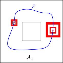
Figure 1: Graphical idea of the proof. The blue curve represents a contour $P$ where the GFF is bigger than $-u$. The red square annuli surrounding points in $P$ are the “good” annuli (such annuli exist for every $z\in P$). Any path between the inner and outer boundaries of $\mathcal{A}_{n}$ has to cross logarithmically many of the red annuli.

1.4 Notational conventions

We write $\mathbbm{N}=\{1,2,3,\dots\}$ and $\mathbbm{N}_{0}=\mathbbm{N}\cup\{0\}$.

For $a<b$, we define the discrete interval $[a,b]_{\mathbbm{Z}}:=[a,b]\cap\mathbbm{Z}$.

If $f:(0,\infty)\rightarrow\mathbbm{R}$ and $g:(0,\infty)\rightarrow(0,\infty)$, we say that $f(\varepsilon)=O_{\varepsilon}(g(\varepsilon))$ (resp. $f(\varepsilon)=o_{\varepsilon}(g(\varepsilon))$) as $\varepsilon\rightarrow 0$ if $f(\varepsilon)/g(\varepsilon)$ remains bounded (resp. tends to zero) as $\varepsilon\rightarrow 0$. We similarly define $O(\cdot)$ and $o(\cdot)$ errors as a parameter goes to infinity.

If $f,g:(0,\infty)\rightarrow[0,\infty)$, we say that $f(\varepsilon)\preceq g(\varepsilon)$ if there is a constant $C>0$ (independent from $\varepsilon$ and possibly from other parameters of interest) such that $f(\varepsilon)\leq Cg(\varepsilon)$. We write $f(\varepsilon)\asymp g(\varepsilon)$ if $f(\varepsilon)\preceq g(\varepsilon)$ and $g(\varepsilon)\preceq f(\varepsilon)$.

We will often specify any requirements on the dependencies on rates of convergence in $O(\cdot)$ and $o(\cdot)$ errors, implicit constants in $\preceq$, etc., in the statements of lemmas/propositions/theorems, in which case we implicitly require that errors, implicit constants, etc., appearing in the proof satisfy the same dependencies.

2 Level set percolation for the GFF

Let $\mathcal{A}_{n}$ be as in Section 1.1. We define a path around $\mathcal{A}_{n}$ to be a nearest-neighbor path in $\mathbbm{Z}^{2}$ which disconnects the inner and outer boundaries of $\mathcal{A}_{n}$. We similarly define a path across $\mathcal{A}_{n}$ to be a nearest-neighbor path in $\mathbbm{Z}^{2}$ between the inner and outer boundaries of $\mathcal{A}_{n}$.

In this section, we give the first lower bound for the LFPP distance between the two boundaries of a (topological) annulus. In particular, we will show that uniformly in $n$ the probability that any path across $\mathcal{A}_{n}$ hits at least one point where $h_{n}>-u$ goes to $1$ as $u\to\infty$. To do this, we will study the probability that there is a path around $\mathcal{A}_{n}$ where $h_{n}>-u$.

Proposition 2.1.

Let $h_{n}$ be a 0-boundary GFF on $\mathcal{B}_{n}$ as in (1.1). There is a universal constant $c>0$ such that for each $n\in\mathbbm{N}$ and each $u>0$,

$$\mathbbm{P}\mathopen{}\mathclose{{}\left[\text{there is a path $P$ around $\mathcal{A}_{n}$ such that $h_{n}\geq-u$ on $P$}}\right]\geq 1-e^{-cu^{2}}.$$

Proposition 2.1 is one of several results in the literature concerning percolation for level sets of the GFF, see, e.g., [AS18, DL18, DW18, DWW20, LW21].

To prove Proposition 2.1, we are going to use a version of the so-called second generalized Ray-Knight theorem from [ALS20]. As the result is not so easy to state, we will simplify it so that we only have to introduce the objects that are strictly necessary for our proof. The exposition of this result is based on Section 2.2 and 2.3 of [ALS20]. For further discussion of the second generalized Ray-Knight theorem, see [Szn12, Chapter 2].

Remark 2.2.

We expect that one can also give an alternative proof of Proposition 2.1 using [DL18, Proposition 4] (which gives an analog of Proposition 2.1 for paths across $\mathcal{A}_{n}$ instead of paths around $\mathcal{A}_{n}$) together with an RSW argument in a similar spirit to the one of [Tas16]. However, we think that the proof we provide here is much shorter and more direct than what this alternative proof would be.

For $x,y\in\mathcal{B}_{n}$, we define $\Gamma^{\mathcal{B}_{n},x,y}$ to be the set of nearest-neighbor paths going from $x$ to $y$ such that all the steps (except maybe the first and the last) remain in the interior of $\mathcal{B}_{n}$. For each $k\in\mathbbm{N}$, we define the non-probability measure $\mu_{k}^{x,y}$ as the measure that assigns mass $4^{-k}$ to each path in $\Gamma^{\mathcal{B}_{n},x,y}$ with length equal to $k$. We also define

$$\nu_{\operatorname{exc}}=\frac{1}{2}\sum_{k=0}^{\infty}\sum_{x,y\in\partial\mathcal{B}_{n}}\mu_{k}^{x,y},$$

that is to say the measure that gives mass $4^{-n}$ to each path $P$ of length $n$ that connects points in $\partial\mathcal{B}_{n}$.

Let $\Xi^{u}$ be a Poisson point process of intensity $u^{2}\nu_{\operatorname{exc}}$. We state now a simplified version of [ALS20, Proposition 2.4]. This proposition is an improvement of the second generalized Ray-Knight theorem and is proven using the techniques of [Lup16].

Theorem 2.3.

There exists a coupling between ${\Xi}^{u}$ and $h_{n}$ such that $h_{n}\geq-u$ on the union of the paths in $\Xi^{u}$.

Proof.

This theorem follows by applying Proposition 2.4 of [ALS20] (which concerns a coupling of a GFF on the so-called metric graph associated with $\mathcal{B}_{n}$) and using the fact that the restriction of the metric graph GFF to the vertices of $\mathcal{B}_{n}$ is a discrete GFF and that the restriction of a PPP of metric graph excursions is a PPP with intensity $\nu_{\text{exc}}$. The fact that the $h_{n}\geq-u$ on each path in $\Xi^{u}$ follows from the third bullet point of that proposition. ∎

We can now prove Proposition 2.1.

Proof of Proposition 2.1.

Thanks to Theorem 2.3, we only need to show that the measure $\nu_{\operatorname{exc}}$ gives positive mass (uniformly in $n$) to paths $P$ that have a subpath $\hat{P}\subseteq P$ which is a path around $\mathcal{A}_{n}$.

To prove this, we first note that for each $\delta>0$, the measure $\nu_{\operatorname{exc}}$ restricted to loops of length longer than $\delta 2^{2n}$ converges weakly, under appropriate scaling, as $n\to\infty$ to a non-zero measure supported on paths in $[-1,1]^{2}$ that only intersect the boundary of $[-1,1]^{2}$ only at their starting and ending points; see [ALS20, Lemma 4.6] for a precise statement. The fact that this limiting measure is supported on paths inside $[-1,1]^{2}$ follows from the explicit definition of the limiting measure given in [ALS20] just before Proposition 3.7.

Because of the nature of the limiting measure, there exists $\epsilon>0$ such that for every $n\in\mathbbm{N}$, $\nu_{\operatorname{exc}}$ gives (uniformly in $n$) positive mass to paths that get to distance at least $\epsilon 2^{n}$ from $\partial\mathcal{B}_{n}$.

Consider now the restriction of $\nu_{\operatorname{exc}}$ to paths which get to distance $\varepsilon 2^{n}$ from $\partial\mathcal{B}_{n}$, normalized to be a probability measure. If $P$ is sampled from this probability measure, then by the definition of $\nu_{\operatorname{exc}}$, the law of $P$ is that of a simple random walk on $\mathcal{B}_{n}$ started from a random point of $\partial\mathcal{B}_{n}$, stopped at the first positive time when it hits $\partial\mathcal{B}_{n}$, and conditioned to get to distance at least $\varepsilon 2^{n}$ from $\partial\mathcal{B}_{n}$ before this time. Let $\tau$ be the first time at which $P$ gets to distance $\varepsilon 2^{n}$ from $\partial\mathcal{B}_{n}$. If we condition on $P|_{[0,\tau]_{\mathbbm{Z}}}$, then the conditional law of the rest of $P$ is that of a simple random walk on $\mathcal{B}_{n}$ started from $P(\tau)$ and stopped upon hitting $\partial\mathcal{B}_{n}$. By the convergence of simple random walk to Brownian motion, it follows that $P$ has uniformly positive probability to make a loop in $\mathcal{A}_{n}$ which disconnects the inner and outer boundaries of $\mathcal{A}_{n}$.

Combining the two preceding paragraphs shows that $\nu_{\operatorname{exc}}$ assigns positive mass to paths which make a loop in $\mathcal{A}_{n}$ which disconnects the inner and outer boundaries of $\mathcal{A}_{n}$, as required. ∎

Remark 2.4.

The limit of the measure $\nu_{exc}$ is called excursion measure, and it is the Brownian analogue of $\nu_{exc}$. For the details of the topology of the convergence, see Section 4.1 of [ALS20].

3 Proof of Theorem 1.1

3.1 Setup and outline

For $z\in\mathbbm{Z}^{2}$ and $n>0$, we write

$$\mathcal{B}_{n}(z):=z+[-2^{n},2^{n}]_{\mathbbm{Z}}^{2}\quad\text{and}\quad\mathcal{B}_{n}^{\circ}(z):=z+[-2^{n}-1,2^{n}-1]_{\mathbbm{Z}}^{2}$$ (3.1)

for the discrete squares of side length $2^{n+1}$ and $2^{n+1}-2$, respectively, centered at $z$. In the notation of Section 1.1, we have $\mathcal{B}_{n}=\mathcal{B}_{n}(0)$.

As in Theorem 1.1, let $h_{n}$ be a discrete GFF on the square $\mathcal{B}_{n}$. For $k\in[0,n-1]_{\mathbbm{Z}}$, $z\in\mathcal{B}_{n}$ such that $\mathcal{B}_{n-k}(z)\subset\mathcal{B}_{n}$, and $u\in\mathcal{B}_{n-k}(z)$, we define

$$\mathfrak{h}_{n,k}^{z}(u):=\mathbbm{E}\mathopen{}\mathclose{{}\left[h_{n}(u)\,|\,h_{n}|_{\mathcal{B}_{n}\setminus\mathcal{B}_{n-k}^{\circ}(z)}}\right]$$ (3.2)

and

$$\mathring{h}_{n,k}^{z}(u):=h_{n}(u)-\mathfrak{h}_{n,k}^{z}(u).$$ (3.3)

Then $\mathfrak{h}_{n,k}^{z}$ is discrete harmonic on $\mathcal{B}_{n-k}^{\circ}(z)$, $\mathring{h}_{n,k}^{z}$ is a zero-boundary discrete GFF on $\mathcal{B}_{n-k}(z)$, $\mathfrak{h}_{n,k}^{z}$ is determined by $h_{n}|_{\mathcal{B}_{n}\setminus\mathcal{B}_{n-k}^{\circ}(z)}$, and $\mathring{h}_{n,k}^{z}$ is independent from $h_{n}|_{\mathcal{B}_{n}\setminus\mathcal{B}_{n-k}^{\circ}(z)}$.

We define $\mathring{D}_{n,k}^{z}$ to be the LFPP metric associated with $\mathring{h}_{n,k}^{z}$, i.e., the metric on $\mathcal{B}_{n-k}(z)$ which is defined as in (1.2) with $\mathring{h}_{n,k}^{z}$ in place of $h_{n}$.

We also define the discrete square annulus

$$\mathcal{A}_{n,k}(z):=\mathcal{B}_{n-k-1/2}(z)\setminus\mathcal{B}_{n-k-1}(z).$$ (3.4)

In the notation of Theorem 1.1, we have $\mathcal{A}_{n}=\mathcal{A}_{n,0}(0)$ and $z+\mathcal{A}_{n-k}=\mathcal{A}_{n,k}(z)$. As in the discussion just above Theorem 1.1, we define $D_{n}\mathopen{}\mathclose{{}\left(\text{across $\mathcal{A}_{n,k}(z)$}}\right)$ to be the minimum $D_{n}$-length of a nearest-neighbor path in $\mathbbm{Z}^{2}$ between the inner and outer boundaries of $\mathcal{A}_{n,k}(z)$. We similarly define $\mathring{D}_{n,k}^{z}\mathopen{}\mathclose{{}\left(\text{around $A_{n,k}(z)$}}\right)$.

The strategy of the proof of Theorem 1.1 is to use Proposition 2.1 to show that any path across $\mathcal{A}_{n}$ has to cross many sets at different scales on which the values of $h_{n}$ are bounded below. More precisely, let $C>1$ be a large universal constant and let $K\in\mathbbm{N}$ be a large constant, to be chosen later in a manner depending only on $\xi$. Say that a point $z\in\mathcal{B}_{n}$ is good if there are at least $3K/8$ values of $k\in[K/2,K-1]_{\mathbbm{Z}}$ for which $\min_{u\in\mathcal{A}_{n,k}(z)}\mathfrak{h}_{n,k}^{z}(u)\geq-C$. In other words, $z$ is good if the harmonic part of the field is bounded below at “most” scales.

The goal of Section 3.2 is to show that with high probability, every path across $\mathcal{A}_{n}$ hits a square of the form $\mathcal{B}_{n-K}(z)$ for some good $z$ (Lemma 3.1). To do this, we first observe that if $z$ is not good, then there are at least $K/4$ “bad” scales where $\min_{u\in\mathcal{A}_{n,k}(z)}\mathfrak{h}_{n,k}^{z}(u)\leq-C$. Using Proposition 2.1 and a comparison between the maximum and minimum values of $\mathfrak{h}_{n,k}^{z}$ on $\mathcal{A}_{n,k}(z)$ (Lemma 3.2) we will show that there is a constant $C^{\prime}>C$ such that the following is true. For each of these bad scales, there is a positive chance that there is a path $P_{k}$ around $\mathcal{A}_{n,k}(z)$ such that $h_{n}<-C^{\prime}$ on $P_{k}$. Using the independence between the field at different scales (Corollary 3.5), we can show that for a bad $z$ it holds with very high probability (high enough to take a union bound over all $z\in 2^{n-k-1}\mathbbm{Z}^{2}$) that such a path $P_{k}$ exists for at least one of the $K/4$ bad scales.

By Proposition 2.1, with high probability there is a path $P$ around $\mathcal{A}_{n}$ on which $h_{n}\geq-C^{\prime}$. The path $P$ cannot hit $\mathcal{B}_{n-K}(z)$ for any bad point $z$, since otherwise it would have to cross one of the paths $P_{k}$ on which $h_{n}<-C^{\prime}$ (Lemma 3.6). This implies that $P$ has to be covered by squares of the form $\mathcal{B}_{n-K}(z)$ for good points $z$. Since any path across $\mathcal{A}_{n}$ has to cross $P$, this shows that any path across $\mathcal{A}_{n}$ has to hit $\mathcal{B}_{n-K}(z)$ for some good point $z$, as required.

In Section 3.3, we will conclude the proof of Theorem 1.1 by applying the result of Section 3.2 at multiple scales via an inductive argument. Suppose that $n\in\mathbbm{N}$, $R>0$, and we have shown that for all $k\in[K/2,K-1]_{\mathbbm{Z}}$, it holds with high probability that $D_{n-k}\mathopen{}\mathclose{{}\left(\text{across $\mathcal{A}_{n}$}}\right)\geq R$. Since $\mathring{h}_{n,k}^{z}$ has the same law as $h_{n-k}$ up to a spatial translation, this show that for each $z\in\mathcal{A}_{n}$, it holds with high probability that (in the notation defined just above) we have $\mathring{D}_{n,k}^{z}\mathopen{}\mathclose{{}\left(\text{across $\mathcal{A}_{n,k}(z)$}}\right)\geq R$. By using independence across scales (Corollary 3.5 again), we get that for each $z\in\mathcal{A}_{n}$, it holds with high probability (high enough for a union bound) that there are at least $3K/8$ scales $k\in[K/2,K-1]_{\mathbbm{Z}}$ for which $\mathring{D}_{n,k}^{z}\mathopen{}\mathclose{{}\left(\text{across $\mathcal{A}_{n,k}(z)$}}\right)\geq R$.

If $z$ is good in the sense described above, then by the preceding paragraph there are at least $K/2-K/8-K/8=K/4$ scales $k\in[K/2,K-1]_{\mathbbm{Z}}$ which are “very good” in the sense that $\mathring{D}_{n,k}^{z}\mathopen{}\mathclose{{}\left(\text{across $\mathcal{A}_{n,k}(z)$}}\right)\geq R$ and $\min_{u\in\mathcal{A}_{n,k}(z)}\mathfrak{h}_{n,k}^{z}(u)\geq-C$. For each very good scale $k$, the $D_{n}$-distance across $\mathcal{A}_{n,k}(z)$ is at least $e^{-\xi C}R$. Since any path across $\mathcal{A}_{n}$ has to hit $\mathcal{B}_{n-K}(z)$ for some good $z$, each such path has to cross at least $K/4$ of these very good scales. This shows that with high probability, $D_{n}\mathopen{}\mathclose{{}\left(\text{across $\mathcal{A}_{n}$}}\right)\geq\frac{1}{4}Ke^{-\xi C}R$ (Lemma 3.7). Making an appropriate choice of $K$ and $R$ and iterating this estimate gives Theorem 1.1.

3.2 Existence of squares where the field is of constant order at many scales

The goal of this subsection is to prove the following lemma; see Section 3.1 for an outline of the proof of the lemma and an explanation of its role in the proof of Theorem 1.1.

Lemma 3.1.

Fix $\delta>0$. There exists $C>0$ and $K_{*}\in\mathbbm{N}$ depending only on $\delta$ such that for each $n,K\in\mathbbm{N}$ with $K_{*}\leq K\leq n-1$, it holds with probability at least $1-\delta$ that the following is true. Each path across $\mathcal{A}_{n}$ hits a square of the form $\mathcal{B}_{n-K}(z)$ for some $z\in(2^{n-K-1}\mathbbm{Z}^{2})\cap\mathcal{B}_{n}$ with the following property: there are at least $(1/2-\delta)K$ values of $k\in[K/2,K-1]_{\mathbbm{Z}}$ for which $\min_{u\in\mathcal{A}_{n,k}(z)}\mathfrak{h}_{n,k}^{z}(u)\geq-C$.

It is easier to lower-bound $\max_{u\in\mathcal{A}_{n,k}(z)}\mathfrak{h}_{n,k}^{z}(u)$ than it is to lower-bound $\min_{u\in\mathcal{A}_{n,k}(z)}\mathfrak{h}_{n,k}^{z}(u)$. The following lemma will allow us to convert between the max and the min.

Lemma 3.2.

There are universal constants $c_{0},c_{1}>0$ such that for each $n\in\mathbbm{N}$, each $K\in[2,n-1]_{\mathbbm{Z}}$, each $z\in\mathcal{B}_{n-1/2}$, and each $C>1$,

$$\mathbbm{P}\mathopen{}\mathclose{{}\left[\sum_{k=2}^{K}\max_{u,v\in\mathcal{A}_{n,k}(z)}(\mathfrak{h}_{n,k}^{z}(u)-\mathfrak{h}_{n,k}^{z}(v))>c_{0}K+C}\right]\leq c_{0}e^{-c_{1}C}.$$ (3.5)

We note that a similar estimate to Lemma 3.2 is proven for the continuum GFF in [MQ20, Proposition 4.3]. The proof of Lemma 3.2 is based on standard Gaussian estimates (namely, the Borell-TIS inequality and Fernique’s criterion). We will need the following basic variance estimate for $\mathfrak{h}_{n,k}^{z}$, which is an immediate consequence of [BDZ16, Lemma 3.10] (applied with $\delta$ equal to a universal constant).

Lemma 3.3 (​​[BDZ16]).

There is a universal constant $c>0$ such that for each $n\in\mathbbm{N}$, each $z\in\mathcal{B}_{n}$ with $\mathcal{B}_{n-k}(z)\subset\mathcal{B}_{n}$, and each $u,v\in\mathcal{B}_{n-k-1/2}(z)$,

$$\mathbbm{E}\mathopen{}\mathclose{{}\left[\mathopen{}\mathclose{{}\left(\mathfrak{h}_{n,k}^{z}(u)-\mathfrak{h}_{n,k}^{z}(v)}\right)^{2}}\right]\leq c\frac{|u-v|}{2^{n-k}}.$$ (3.6)

Proof of Lemma 3.2.

Observe that

$$\sum_{k=2}^{K}\max_{u,v\in\mathcal{A}_{n,k}(z)}(\mathfrak{h}_{n,k}^{z}(u)-\mathfrak{h}_{n,k}^{z}(v))$$

$$\qquad=\max\mathopen{}\mathclose{{}\left\{\sum_{k=2}^{K}\mathopen{}\mathclose{{}\left(\mathfrak{h}_{n,k}^{z}(u_{k})-\mathfrak{h}_{n,k}^{z}(v_{k})}\right):u_{2},v_{2}\in\mathcal{A}_{n,2}(z),\dots,u_{K},v_{K}\in\mathcal{A}_{n,K}(z)}\right\},$$ (3.7)

so the random variable which we are interested in is the maximum of a centered Gaussian process. We will now estimate the quantity in (3.2) using the Borell-TIS inequality.

We first estimate the expectation of the maximum. By Lemma 3.3 and Fernique’s inequality [Fer75] (see, e.g., [BDZ16, Lemma 3.5]), for each $k\in[2,K]_{\mathbbm{Z}}$,

$$\mathbbm{E}\mathopen{}\mathclose{{}\left[\max_{u\in\mathcal{A}_{n,k}(z)}|\mathfrak{h}_{n,k}^{z}(u)|}\right]\preceq 1,$$

with a universal implicit constant. Summing this estimate gives

$$\mathbbm{E}\mathopen{}\mathclose{{}\left[\sum_{k=2}^{K}\max_{u\in\mathcal{A}_{n,k}(z)}(\mathfrak{h}_{n,k}^{z}(u)-\mathfrak{h}_{n,k}^{z}(v))}\right]\preceq K.$$ (3.8)

We now need to estimate the pointwise variance of the Gaussian process whose maximum we are taking in (3.2). For any fixed choice of $u_{2},v_{2}\in\mathcal{A}_{n,2}(z),\dots,u_{K},v_{K}\in\mathcal{A}_{n,K}(z)$,

$$\operatorname{Var}\mathopen{}\mathclose{{}\left(\sum_{k=2}^{K}(\mathfrak{h}_{n,k}^{z}(u_{k})-\mathfrak{h}_{n,k}^{z}(v_{k}))}\right) =2\sum_{j=2}^{K-1}\sum_{k=j+1}^{K}\mathbbm{E}\mathopen{}\mathclose{{}\left[(\mathfrak{h}_{n,j}^{z}(u_{j})-\mathfrak{h}_{n,j}^{z}(v_{j}))(\mathfrak{h}_{n,k}^{z}(u_{k})-\mathfrak{h}_{n,k}^{z}(v_{k}))}\right]$$

$$\qquad+\sum_{k=2}^{K}\mathbbm{E}\mathopen{}\mathclose{{}\left[(\mathfrak{h}_{n,k}^{z}(u_{k})-\mathfrak{h}_{n,k}^{z}(v_{k}))^{2}}\right].$$ (3.9)

To estimate the first sum on the right in (3.2), we note that for $j<k$,

$$\mathbbm{E}\mathopen{}\mathclose{{}\left[(\mathfrak{h}_{n,j}^{z}(u_{j})-\mathfrak{h}_{n,j}^{z}(v_{j}))(\mathfrak{h}_{n,k}^{z}(u_{k})-\mathfrak{h}_{n,k}^{z}(v_{k}))}\right]$$

$$\qquad=\mathbbm{E}\mathopen{}\mathclose{{}\left[(\mathfrak{h}_{n,j}^{z}(u_{j})-\mathfrak{h}_{n,j}^{z}(v_{j}))\mathbbm{E}\mathopen{}\mathclose{{}\left[(\mathfrak{h}_{n,k}^{z}(u_{k})-\mathfrak{h}_{n,k}^{z}(v_{k}))\,|\,\mathfrak{h}_{n,j}^{z}}\right]}\right].$$ (3.10)

Recall that $h_{n}|_{\mathcal{B}_{n-j}(z)}$ is the sum of $\mathfrak{h}_{n,j}^{z}$ and an independent zero-boundary GFF on $\mathcal{B}_{n-j}(z)$. Hence, $\mathbbm{E}\mathopen{}\mathclose{{}\left[(\mathfrak{h}_{n,k}^{z}(u_{k})-\mathfrak{h}_{n,k}^{z}(v_{k}))\,|\,\mathfrak{h}_{n,j}^{z}}\right]=\mathfrak{h}_{n,j}^{z}(u_{k})-\mathfrak{h}_{n,j}^{z}(v_{k})$. We can therefore bound the right side of (3.2) by applying the Cauchy-Schwarz inequality, followed by Lemma 3.3 (with $j$ in place of $k$), to get

$$\mathbbm{E}\mathopen{}\mathclose{{}\left[(\mathfrak{h}_{n,j}^{z}(u_{j})-\mathfrak{h}_{n,j}^{z}(v_{j}))(\mathfrak{h}_{n,k}^{z}(u_{k})-\mathfrak{h}_{n,k}^{z}(v_{k}))}\right] \leq\mathbbm{E}\mathopen{}\mathclose{{}\left[\mathopen{}\mathclose{{}\left(\mathfrak{h}_{n,j}^{z}(u_{j})-\mathfrak{h}_{n,j}^{z}(v_{j})}\right)^{2}}\right]^{1/2}\mathbbm{E}\mathopen{}\mathclose{{}\left[\mathopen{}\mathclose{{}\left(\mathfrak{h}_{n,j}^{z}(u_{k})-\mathfrak{h}_{n,j}^{z}(v_{k})}\right)^{2}}\right]^{1/2}$$

$$\preceq\frac{|u_{j}-v_{j}|^{1/2}|u_{k}-v_{k}|^{1/2}}{2^{n-j}}$$

$$\preceq 2^{-(k-j)/2}$$ (3.11)

with a universal implicit constant. Note that in the last line, we used that $|u_{k}-v_{k}|\preceq 2^{n-k}$ for each $k\in[2,K]_{\mathbbm{Z}}$.

We now use (3.2) to bound the first sum on the right side of (3.2) and Lemma 3.3 to bound the second sum. This leads to

$$\operatorname{Var}\mathopen{}\mathclose{{}\left(\sum_{k=2}^{K}(\mathfrak{h}_{n,k}^{z}(u_{k})-\mathfrak{h}_{n,k}^{z}(v_{k}))}\right) \preceq\sum_{j=2}^{K-1}\sum_{k=j+1}^{K}2^{-(k-j)/2}+\sum_{k=2}^{K}\frac{|u_{k}-v_{k}|}{2^{n-k}}$$

$$\leq\sum_{j=2}^{K-1}O(1)+\sum_{k=2}^{K}O(1)$$

$$\preceq K.$$ (3.12)

By (3.8) and (3.2), we can apply the Borell-TIS inequality [Bor75, SCs74] (see, e.g., [AT07, Theorem 2.1.1]) to bound the maximum on the right side of (3.2). This gives (3.5). ∎

Since the zero-boundary GFF $\mathring{h}_{n,k}^{z}$ from (3.3) is independent from $h_{n}|_{\mathcal{B}_{n}\setminus\mathcal{B}_{n-k}^{\circ}(z)}$, we can get independence for certain events defined in terms of $\mathring{h}_{n,k}^{z}$, as the following lemma demonstrates.

Lemma 3.4.

Let $n\in\mathbbm{N}$, let $z\in\mathcal{B}_{n-1/2}$, and let $\{E_{k}\}_{k\in[2,n-1]_{\mathbbm{Z}}}$ be events such that each $E_{k}$ is measurable w.r.t. $\sigma\mathopen{}\mathclose{{}\left(\mathring{h}_{n,k}^{z}|_{\mathcal{A}_{n,k}(z)}}\right)$. Then the events $\{E_{k}\}_{k\in[2,n-1]_{\mathbbm{Z}}}$ are independent.

Proof.

For each $k\in[2,n-1]_{\mathbbm{Z}}$,

$$E_{k}\in\sigma\mathopen{}\mathclose{{}\left(\mathring{h}_{n,k}^{z}|_{\mathcal{A}_{n,k}(z)}}\right)\subset\sigma\mathopen{}\mathclose{{}\left(h_{n}|_{\mathcal{B}_{n}\setminus\mathcal{B}_{n-k-1}^{\circ}(z)}}\right).$$

On the other hand, $\mathring{h}_{n,k}^{z}$, hence also $E_{k}$, is independent from $h_{n}|_{\mathcal{B}_{n}\setminus\mathcal{B}_{n-k}^{\circ}(z)}$. This implies the lemma statement. ∎

The lemma above is useful to estimate the number of values of $k$ for which $E_{k}$ occurs. The particular estimate we need is the following corollary.

Corollary 3.5.

For each $a\in(0,1)$ and $b>1$, there exists $p=p(a,b)\in(0,1)$ such that the following is true. Let $K_{1},K_{2},n\in\mathbbm{N}$ with $2\leq K_{1}<K_{2}\leq n-1$ and let $z\in\mathcal{B}_{n-1/2}$. For $k\in[K_{1},K_{2}]_{\mathbbm{Z}}$, let $E_{k}$ be an event which is measurable w.r.t. $\sigma\mathopen{}\mathclose{{}\left(\mathring{h}_{n,k}^{z}|_{\mathcal{A}_{n,k}(z)}}\right)$ and satisfies $\mathbbm{P}[E_{k}]\geq p$. Then

$$\mathbbm{P}\mathopen{}\mathclose{{}\left[\#\mathopen{}\mathclose{{}\left\{k\in[K_{1},K_{2}]_{\mathbbm{Z}}:E_{k}\>\text{occurs}}\right\}\geq a(K_{2}-K_{1})}\right]\geq 1-2^{-b(K_{2}-K_{1})}.$$ (3.13)

Proof.

The corollary follows from Lemma 3.4 together with a basic tail estimate for the binomial distribution. ∎

The following lemma is the key input in the proof of Lemma 3.1.

Lemma 3.6.

Let $\delta>0$ and $A>1$. There are constants $C,c>1$ depending only on $\delta$ and $A$ such that for each $n,K\in\mathbbm{N}$ with $2/\delta\leq K\leq n-1$ and each $z\in\mathcal{A}_{n}$, the probability that the following two conditions both hold simultaneously is at most $c2^{-3K}$:

1. There are at least $\delta K$ values of $k\in[K/2,K-1]_{\mathbbm{Z}}$ for which $\min_{u\in\mathcal{A}_{n,k}(z)}\mathfrak{h}_{n,k}^{z}(u)\leq-C$.

2. There is a path $P$ around $\mathcal{A}_{n}$ such that $h_{n}\geq-A$ on $P$ and $P\cap\mathcal{B}_{n-K}(z)\not=\emptyset$.

We note that a path $P$ as in Lemma 3.6 exists with high probability when $A$ is large by Proposition 2.1.

Proof of Lemma 3.6.

Fix a constant $C_{1}>1$ to be chosen later, in a manner depending only on $\delta$ and $A$. For $k\in\mathbbm{N}$, let $E_{k}=E_{n,k}(z,C_{1})$ be the event that there is a path $P_{k}$ around $\mathcal{A}_{n,k}(z)$ such that $\mathring{h}_{n,k}^{z}\leq C_{1}-A-1$ on $P_{k}$. Since $\mathring{h}_{n,k}^{z}$ is a zero-boundary GFF on $\mathcal{B}_{n-k}(z)$, we can apply Proposition 2.1 with $n-k$ in place of $n$ and $-\mathring{h}_{n,k}^{z}$ in place of $h_{n}$. This shows that for each $p\in(0,1)$ there exists $C_{1}=C_{1}(p,A)>1$ such that for this choice of $C_{1}$, we have $\mathbbm{P}[E_{k}]\geq p$ for every $k\in[2,K]_{\mathbbm{Z}}$ and every $z\in\mathcal{A}_{n}$. By Corollary 3.5, if we choose $p$ to be sufficiently close to 1 (depending on $\delta$ and $A$) then

$$\mathbbm{P}\mathopen{}\mathclose{{}\left[\#\mathopen{}\mathclose{{}\left\{k\in[K/2,K-1]_{\mathbbm{Z}}:E_{k}\>\text{occurs}}\right\}\geq(1/2-\delta/4)K}\right]\geq 1-2^{-3K}.$$ (3.14)

By Lemma 3.2 (applied with a large multiple of $K$ in place of $C$), there exists $C_{2}=C_{2}(\delta)>1$ and $c_{0}>0$ such that

$$\mathbbm{P}\mathopen{}\mathclose{{}\left[\sum_{k=2}^{K-1}\max_{u,v\in\mathcal{A}_{n,k}(z)}(\mathfrak{h}_{n,k}^{z}(u)-\mathfrak{h}_{n,k}^{z}(v))\leq\frac{C_{2}\delta}{4}K}\right]\geq 1-c_{0}2^{-3K}.$$ (3.15)

If the event in (3.15) occurs then there are at most $\delta K/4$ values of $k\in[2,K]_{\mathbbm{Z}}$ for which $\max_{u,v\in\mathcal{A}_{n,k}(z)}(\mathfrak{h}_{n,k}^{z}(u)-\mathfrak{h}_{n,k}^{z}(v))>C_{2}$. Therefore,

$$\mathbbm{P}\mathopen{}\mathclose{{}\left[\#\mathopen{}\mathclose{{}\left\{k\in[K/2,K-1]_{\mathbbm{Z}}:\max_{u,v\in\mathcal{A}_{n,k}(z)}(\mathfrak{h}_{n,k}^{z}(u)-\mathfrak{h}_{n,k}^{z}(v))\leq C_{2}}\right\}\geq(1/2-\delta/4)K}\right]\geq 1-c_{0}2^{-3K}.$$ (3.16)

Henceforth assume that the events in (3.14) and (3.16) occur, which happens with probability at least $1-c2^{-3K}$ for a constant $c>1$ depending only on $\delta,A$. Let $C:=C_{1}+C_{2}$. To prove the lemma, it suffices to show that if condition 1 in the lemma statement holds with this choice of $C$, then condition 2 does not hold.

If there $\delta K$ values of $k\in[K/2,K-1]_{\mathbbm{Z}}$ for which $\min_{u\in\mathcal{A}_{n,k}(z)}\mathfrak{h}_{n,k}^{z}(u)\leq-C$, then the events in (3.14) and (3.16) imply that there must be at least $\lfloor\delta K/2\rfloor$ values of $k\in[K/2,K-1]_{\mathbbm{Z}}$ for which $E_{k}$ occurs, $\max_{u,v\in\mathcal{A}_{n,k}(z)}(\mathfrak{h}_{n,k}^{z}(u)-\mathfrak{h}_{n,k}^{z}(v))\leq C_{2}$, and $\min_{u\in\mathcal{A}_{n,k}(z)}\mathfrak{h}_{n,k}^{z}(u)\leq-C$.

Since $K\geq 2/\delta$, we have $\lfloor\delta K/2\rfloor\geq 1$. Hence we can choose one value of $k$ as in the preceding paragraph. Let $P_{k}$ be the path around $\mathcal{A}_{n,k}(z)$ as in the definition of $E_{k}$, so that $\mathring{h}_{n,k}^{z}\leq C_{1}-A-1$ on $P_{k}$. Since $k\in[K/2,K-1]_{\mathbbm{Z}}$, the path $P_{k}$ disconnects $\mathcal{B}_{n-K}(z)$ from $\infty$ and intersects $\mathcal{A}_{n}$. Hence every path around $\mathcal{A}_{n}$ which intersects $\mathcal{B}_{n-K}(z)$ must also intersect $P_{k}$. To prove the lemma, it therefore suffices to show that $\max_{z\in P_{k}}h_{n}(u)<-A$ (so that there can be no path around $\mathcal{A}_{n}$ which intersects $\mathcal{B}_{n-K}(z)$ on which $h_{n}\geq-A$). Indeed, we have

$$\max_{u\in P_{k}}h_{n}(u) \leq\max_{u\in P_{k}}\mathring{h}_{n,k}^{z}(u)+\max_{u\in\mathcal{A}_{n,k}(z)}\mathfrak{h}_{n,k}^{z}(u)$$

$$\leq\max_{u\in P_{k}}\mathring{h}_{n,k}^{z}(u)+\min_{u\in\mathcal{A}_{n,k}(z)}\mathfrak{h}_{n,k}^{z}(u)+\max_{u,v\in\mathcal{A}_{n,k}(z)}(\mathfrak{h}_{n,k}^{z}(u)-\mathfrak{h}_{n,k}^{z}(v))$$

$$\leq(C_{1}-A-1)-C+C_{2}\quad\text{(by our choice of $k$)}$$

$$=-A-1\quad\text{(by the definition of $C$)}.$$

∎

Proof of Lemma 3.1.

By Proposition 2.1, we can find $A=A(\delta)>1$ such that with probability at least $1-\delta/2$, there is a path $P$ around $\mathcal{A}_{n}$ such that $h_{n}\geq-A$ on $P$. Let $C=C(\delta/2,A)>1$ be as in Lemma 3.6 for this choice of $A$, with $\delta/2$ in place of $\delta$. By Lemma 3.6 (with $\delta/2$ in place of $\delta$) and a union bound over $O_{K}(2^{2K})$ possible points $z\in(2^{-n-K-1}\mathbbm{Z}^{2})\cap\mathcal{A}_{n}$, there is a constant $c>0$ depending only on $\delta$ such that with probability at least $1-c2^{-K}$, the following is true. For each $z\in 2^{n-K-1}\mathbbm{Z}^{2}$ such that $P$ hits $\mathcal{B}_{n-K}(z)$, there are at most $(\delta/2)K$ values of $k\in[K/2,K-1]_{\mathbbm{Z}}$ for which $\min_{u\in\mathcal{A}_{n,k}(z)}\mathfrak{h}_{n,k}^{z}(u)\leq-C$. Hence for each such $z$, there are at least $(1/2-\delta)K$ values of $k\in[K/3,K-1]_{\mathbbm{Z}}$ for which $\min_{u\in\mathcal{A}_{n,k}(z)}\mathfrak{h}_{n,k}^{z}(u)\geq-C$.

We now choose $K_{*}$ to be large enough so that $c2^{-K_{*}}\leq\delta/2$. Then if $K\geq K_{*}$, it holds with probability at least $1-\delta$ that the path $P$ as above exists and for each $z\in 2^{n-K-1}\mathbbm{Z}^{2}$ such that $P$ hits $\mathcal{B}_{n-K}(z)$, there are at least $(1/2-\delta)K$ values of $k\in[K/2,K-1]_{\mathbbm{Z}}$ for which $\min_{u\in\mathcal{A}_{n,k}(z)}\mathfrak{h}_{n,k}^{z}(u)\geq-C$. Any path in $\mathbbm{Z}^{2}$ from $\partial\mathcal{B}_{n-1}$ to $\partial\mathcal{B}_{n-1/2}$ must cross $P$, so must hit a square of the form $\mathcal{B}_{n-K}(z)$ for some $z\in 2^{n-K-1}\mathbbm{Z}^{2}$ such that $P$ also hits $\mathcal{B}_{n-K}(z)$. But, we know that each $z$ for which $P$ hits $\mathcal{B}_{n-K}(z)$ satisfies the condition in the lemma statement, so this concludes the proof. ∎

3.3 Inductive argument

Theorem 1.1 will be a consequence of the following lemma applied inductively.

Lemma 3.7.

Let $q_{0}\in(0,1)$ be chosen so that the conclusion of Corollary 3.5 holds with $a=3/4$ and $b=6$. For each $q\in[q_{0},1)$, there are constants $C>0$ and $K_{*}\in\mathbbm{N}$ depending only on $q$ such that if $n,K\in\mathbbm{N}$ with $K_{*}\leq K\leq n-1$, then the following is true. If $R>0$ is such that

$$\mathbbm{P}\mathopen{}\mathclose{{}\left[D_{m}\mathopen{}\mathclose{{}\left(\text{across $\mathcal{A}_{m}$}}\right)\geq R}\right]\geq q,\quad\forall m\in[n-K+1,n-K/2]_{\mathbbm{Z}},$$ (3.17)

then

$$\mathbbm{P}\mathopen{}\mathclose{{}\left[D_{n}\mathopen{}\mathclose{{}\left(\text{across $\mathcal{A}_{n}$}}\right)\geq\frac{1}{4}Ke^{-\xi C}R}\right]\geq q.$$ (3.18)

Proof.

Throughout the proof we assume that $n,K\in\mathbbm{N}$ with $K\leq n-1$ and $R>0$ are such that (3.17) holds.

Each of the fields $\mathring{h}_{n,k}^{z}$ for $z\in\mathcal{A}_{n}$ is a zero-boundary GFF on a translated copy of $\mathcal{A}_{n-k}$. Therefore, (3.17) implies that for each $z\in\mathcal{A}_{n}$ and each $k\in[K/2,K-1]_{\mathbbm{Z}}$,

$$\mathbbm{P}\mathopen{}\mathclose{{}\left[\mathring{D}_{n,k}^{z}\mathopen{}\mathclose{{}\left(\text{across $\mathcal{A}_{n,k}(z)$}}\right)\geq R}\right]\geq q;$$ (3.19)

recall that $\mathring{D}_{n,k}^{z}$ is the LFPP metric associated with $\mathring{h}_{n,k}^{z}$, as in Section 3.1. By (3.19), our choice of $q_{0}$, and Corollary 3.5 applied with

$$E_{k}=\mathopen{}\mathclose{{}\left\{\mathring{D}_{n,k}^{z}\mathopen{}\mathclose{{}\left(\text{across $\mathcal{A}_{n,k}(z)$}}\right)\geq R}\right\},$$

there is a universal constant $c>0$ such that for each $z\in\mathcal{A}_{n}$ it holds with probability at least $1-c2^{-3K}$ that there are at least $3K/8$ values of $k\in[K/2,K-1]_{\mathbbm{Z}}$ for which $\mathring{D}_{n,k}^{z}\mathopen{}\mathclose{{}\left(\text{across $\mathcal{A}_{n,k}(z)$}}\right)\geq R$.

By a union bound over $O_{K}(2^{2K})$ points $z\in(2^{-n-K-1}\mathbbm{Z}^{2})\cap\mathcal{A}_{n}$, after possibly increasing $c$ we can arrange that with probability at least $1-c2^{-K}$, it holds for every $z\in(2^{-n-K-1}\mathbbm{Z}^{2})\cap\mathcal{A}_{n}$ that there are at least $3K/8$ values of $k\in[K/2,K-1]_{\mathbbm{Z}}$ for which $\mathring{D}_{n,k}^{z}\mathopen{}\mathclose{{}\left(\text{across $\mathcal{A}_{n,k}(z)$}}\right)\geq R$.

By Lemma 3.1 (applied with $\delta=\min\{1/8,(1-q)/2\}$), there are constants $C>0$ and $K_{0}\in\mathbbm{N}$ depending only on $q$ such that if $K\geq K_{0}$, then with probability at least $1-(1-q)/2$, each path across $\mathcal{A}_{n}$ hits a square of the form $\mathcal{B}_{n-K}(z)$ for some $z\in 2^{n-K-1}\mathbbm{Z}^{2}$ with the following property: there are at least $3K/8$ values of $k\in[K/2,K-1]_{\mathbbm{Z}}$ for which $\min_{u\in\mathcal{A}_{n,k}(z)}\mathfrak{h}_{n,k}^{z}(u)\geq-C$.

Now let $K_{*}=K_{*}(q)\geq K_{0}$ be chosen so that $c2^{-K_{0}}\leq(1-q)/2$. If $K\geq K_{*}$, the combination of the preceding two paragraphs shows that with probability at least $q$, each path across $\mathcal{A}_{n}$ hits a square of the form $\mathcal{B}_{n-K}(z)$ for some $z\in 2^{n-K-1}\mathbbm{Z}^{2}$ with the following property: there are at least $K/4$ values of $k\in[K/2,K-1]_{\mathbbm{Z}}$ for which $\min_{u\in\mathcal{A}_{n,k}(z)}\mathfrak{h}_{n,k}^{z}(u)\geq-C$ and $\mathring{D}_{n,k}^{z}\mathopen{}\mathclose{{}\left(\text{across $\mathcal{A}_{n,k}(z)$}}\right)\geq R$. For each such $k$,

$$D_{n}\mathopen{}\mathclose{{}\left(\text{across $\mathcal{A}_{n,k}(z)$}}\right)\geq\exp\mathopen{}\mathclose{{}\left(\xi\min_{u\in\mathcal{A}_{n,k}(z)}\mathfrak{h}_{n,k}^{z}(u)}\right)\mathring{D}_{n,k}^{z}\mathopen{}\mathclose{{}\left(\text{across $\mathcal{A}_{n-k}(z)$}}\right)\geq e^{-\xi C}R.$$ (3.20)

If a path across $\mathcal{A}_{n}$ hits $\mathcal{B}_{n-K}(z)$, then it must cross each of the annuli $\mathcal{A}_{n,k}(z)$ for $k\in[K/2,K-1]_{\mathbbm{Z}}$ at least once (it must cross each of these annuli twice if $z$ is at distance at least $2^{n-K/2}$ from the boundary of $\mathcal{A}_{n}$). By (3.20), the $D_{n}$-length of each path across $\mathcal{A}_{n}$ is at least $\frac{1}{4}Ke^{-\xi C}R$. Thus (3.18) holds. ∎

Proof of Theorem 1.1.

Let $q\in[q_{0},1)$, $C>0$, and $K_{*}\in\mathbbm{N}$ be as in Lemma 3.7. We will prove the theorem by an inductive argument based on Lemma 3.7. For the base case, we need an a priori lower bound for $D_{n}(\text{across $\mathcal{A}_{n}$})$, which will come from Proposition 2.1.

Step 1: a priori lower bound for annulus crossing distance. By Proposition 2.1, there exists a constant $C^{\prime}>0$ depending only on $q$ such that for each $n\in\mathbbm{N}$, it holds with probability at least $q$ that there is a path $P$ around $\mathcal{A}_{n}$ such that $h_{n}\geq-C^{\prime}$ on $P$. Each path across $\mathcal{A}_{n}$ must cross $P$, so

$$\mathbbm{P}\mathopen{}\mathclose{{}\left[D_{n}\mathopen{}\mathclose{{}\left(\text{across $\mathcal{A}_{n}$}}\right)\geq e^{-\xi C^{\prime}}}\right]\geq q,\quad\forall n\in\mathbbm{N}.$$ (3.21)

Let $K\geq K_{*}$ (to be chosen later in a manner depending only on $\xi$). By (3.21) applied for $n\in[1,K]_{\mathbbm{Z}}$, the condition (3.17) holds with $R=e^{-\xi C^{\prime}}$ for each $n\in[K,2K]_{\mathbbm{Z}}$. By Lemma 3.7,

$$\mathbbm{P}\mathopen{}\mathclose{{}\left[D_{n}\mathopen{}\mathclose{{}\left(\text{across $\mathcal{A}_{n}$}}\right)\geq\frac{1}{4}Ke^{-\xi(C+C^{\prime})}}\right]\geq q,\quad\forall n\in[K,2K]_{\mathbbm{Z}}.$$ (3.22)

This is our desired a priori lower bound.

Step 2: inductive argument. We now let

$$K=K(\xi):=\max\mathopen{}\mathclose{{}\left\{K_{*},16e^{\xi(C+C^{\prime})}+1}\right\}.$$ (3.23)

We will prove by induction on $n$ that for each $n\geq K$,

$$\mathbbm{P}\mathopen{}\mathclose{{}\left[D_{n}\mathopen{}\mathclose{{}\left(\text{across $\mathcal{A}_{n}$}}\right)\geq 2^{n/K}}\right]\geq q.$$ (3.24)

Indeed, it follows from (3.22) and our choice of $K$ that (3.24) holds for all $n\in[K,2K]_{\mathbbm{Z}}$. This gives the base case.

For the inductive step, assume that $n\geq 2K$ and (3.24) has been proven with $n$ replaced by any $m\in[K,n-1]_{\mathbbm{Z}}$. Then (3.17) of Lemma 3.7 holds for our given value of $n$ and with $R=2^{(n-K)/K}$. Therefore, Lemma 3.7 implies that

$$\mathbbm{P}\mathopen{}\mathclose{{}\left[D_{n}\mathopen{}\mathclose{{}\left(\text{across $\mathcal{A}_{n}$}}\right)\geq\frac{1}{4}Ke^{-\xi C}2^{(n-K)/K}}\right]\geq q.$$

By our choice of $K$, we have $\frac{1}{4}Ke^{-\xi C}\geq 4$, so $\frac{1}{4}Ke^{-\xi C}2^{(n-K)/K}\geq 2^{n/K}$. Thus (3.24) holds for $n$. This completes the induction, so we get that (3.24) holds for all $n\geq K$.

By (3.24),

$$\liminf_{n\rightarrow\infty}\mathbbm{P}\mathopen{}\mathclose{{}\left[D_{n}\mathopen{}\mathclose{{}\left(\text{across $\mathcal{A}_{n}$}}\right)\geq 2^{n/K}}\right]\geq q.$$

By (3.23), $(\log 2)/K\geq c_{0}e^{-c_{1}\xi}$ for constants $c_{0},c_{1}>0$ depending only on $q$. This gives (1.4). ∎

References

- [ALS20] J. Aru, T. Lupu, and A. Sepúlveda. The First Passage Sets of the 2D Gaussian Free Field: Convergence and Isomorphisms. Comm. Math. Phys., 375(3):1885–1929, 2020, 1805.09204. MR4091511
- [Ang19] M. Ang. Comparison of discrete and continuum Liouville first passage percolation. Electron. Commun. Probab., 24:Paper No. 64, 12, 2019, 1904.09285. MR4029433
- [APPS20] M. Ang, M. Park, J. Pfeffer, and S. Sheffield. Brownian loops and the central charge of a Liouville random surface. ArXiv e-prints, May 2020, 2005.11845.
- [AS18] J. Aru and A. Sepúlveda. Two-valued local sets of the 2D continuum Gaussian free field: connectivity, labels, and induced metrics. Electron. J. Probab., 23:Paper No. 61, 35, 2018, 1801.03828. MR3827968
- [AT07] R. J. Adler and J. E. Taylor. Random fields and geometry. Springer Monographs in Mathematics. Springer, New York, 2007. MR2319516 (2008m:60090)
- [BDZ16] M. Bramson, J. Ding, and O. Zeitouni. Convergence in law of the maximum of the two-dimensional discrete Gaussian free field. Comm. Pure Appl. Math., 69(1):62–123, 2016, 1301.6669. MR3433630
- [Ber] N. Berestycki. Introduction to the Gaussian Free Field and Liouville Quantum Gravity. Available at https://homepage.univie.ac.at/nathanael.berestycki/articles.html.
- [Bor75] C. Borell. The Brunn-Minkowski inequality in Gauss space. Invent. Math., 30(2):207–216, 1975. MR0399402
- [DDDF20] J. Ding, J. Dubédat, A. Dunlap, and H. Falconet. Tightness of Liouville first passage percolation for . Publ. Math. Inst. Hautes Études Sci., 132:353–403, 2020, 1904.08021. MR4179836
- [DG18] J. Ding and E. Gwynne. The fractal dimension of Liouville quantum gravity: universality, monotonicity, and bounds. Communications in Mathematical Physics, 374:1877–1934, 2018, 1807.01072.
- [DG20] J. Ding and E. Gwynne. Tightness of supercritical Liouville first passage percolation. Journal of the European Mathematical Society, to appear, 2020, 2005.13576.
- [DG21a] J. Ding and E. Gwynne. Regularity and confluence of geodesics for the supercritical Liouville quantum gravity metric. ArXiv e-prints, April 2021, 2104.06502.
- [DG21b] J. Ding and E. Gwynne. Uniqueness of the critical and supercritical Liouville quantum gravity metrics. ArXiv e-prints, September 2021, 2110.00177.
- [DKRV16] F. David, A. Kupiainen, R. Rhodes, and V. Vargas. Liouville quantum gravity on the Riemann sphere. Comm. Math. Phys., 342(3):869–907, 2016, 1410.7318. MR3465434
- [DL18] J. Ding and L. Li. Chemical distances for percolation of planar Gaussian free fields and critical random walk loop soups. Comm. Math. Phys., 360(2):523–553, 2018, 1605.04449. MR3800790
- [DS11] B. Duplantier and S. Sheffield. Liouville quantum gravity and KPZ. Invent. Math., 185(2):333–393, 2011, 1206.0212. MR2819163 (2012f:81251)
- [DW18] J. Ding and M. Wirth. Percolation for level-sets of Gaussian free fields on metric graphs. ArXiv e-prints, July 2018, 1807.11117.
- [DWW20] J. Ding, M. Wirth, and H. Wu. Crossing estimates from metric graph and discrete GFF. ArXiv e-prints, January 2020, 2001.06447.
- [Fer75] X. Fernique. Regularité des trajectoires des fonctions aléatoires gaussiennes. pages 1–96. Lecture Notes in Math., Vol. 480, 1975. MR0413238
- [GHPR20] E. Gwynne, N. Holden, J. Pfeffer, and G. Remy. Liouville quantum gravity with matter central charge in (1, 25): a probabilistic approach. Comm. Math. Phys., 376(2):1573–1625, 2020, 1903.09111. MR4103975
- [GM21] E. Gwynne and J. Miller. Existence and uniqueness of the Liouville quantum gravity metric for . Invent. Math., 223(1):213–333, 2021, 1905.00383. MR4199443
- [GP19] E. Gwynne and J. Pfeffer. Bounds for distances and geodesic dimension in Liouville first passage percolation. Electronic Communications in Probability, 24:no. 56, 12, 2019, 1903.09561.
- [Gwy20] E. Gwynne. Random surfaces and Liouville quantum gravity. Notices Amer. Math. Soc., 67(4):484–491, 2020, 1908.05573. MR4186266
- [Lup16] T. Lupu. From loop clusters and random interlacements to the free field. Ann. Probab., 44(3):2117–2146, 2016, 1402.0298. MR3502602
- [LW21] M. Liu and H. Wu. Scaling limits of crossing probabilities in metric graph GFF. Electron. J. Probab., 26:Paper No. 37, 46, 2021, 2004.09104. MR4235488
- [MQ20] J. Miller and W. Qian. The geodesics in Liouville quantum gravity are not Schramm-Loewner evolutions. Probab. Theory Related Fields, 177(3-4):677–709, 2020, 1812.03913.
- [Pfe21] J. Pfeffer. Weak Liouville quantum gravity metrics with matter central charge . ArXiv e-prints, April 2021, 2104.04020.
- [SCs74] V. N. Sudakov and B. S. Cirel′ son. Extremal properties of half-spaces for spherically invariant measures. Zap. Naučn. Sem. Leningrad. Otdel. Mat. Inst. Steklov. (LOMI), 41:14–24, 165, 1974. Problems in the theory of probability distributions, II. MR0365680
- [Szn12] A.-S. Sznitman. Topics in occupation times and Gaussian free fields, volume 16. European Mathematical Society, 2012.
- [Tas16] V. Tassion. Crossing probabilities for Voronoi percolation. Ann. Probab., 44(5):3385–3398, 2016, 1410.6773. MR3551200