Double layered solutions to the extended Fisher-Kolmogorov P.D.E.

Abstract.

We construct double layered solutions to the extended Fisher-Kolmogorov P.D.E., under the assumption that the set of minimal heteroclinics of the corresponding O.D.E. satisfies a separation condition. The aim of our work is to provide for the extended Fisher-Kolmogorov equation, the first examples of two-dimensional minimal solutions, since these solutions play a crucial role in phase transition models, and are closely related to the De Giorgi conjecture.

1. Introduction and Statements

We consider the extended Fisher-Kolmogorov P.D.E.

(1) $$\Delta^{2}u(t,x)-\beta\Delta u(t,x)+\nabla W(u(t,x))=0,\ u:\mathbb{R}^{2}\to\mathbb{R}^{m}\ m\geq 1,\ \beta>0,\ (t,x)\in\mathbb{R}^{2},$$

where $W$ is a function such that

(2a) $$W\in C^{2}(\mathbb{R}^{m};\mathbb{R}) 2 a^{-} a^{+}$$ is nonnegative, and has exactly zeros and ,

(2b) $$\text{$\nabla^{2}W(u)(\nu,\nu)\geq c$, $\forall u\in\mathbb{R}^{m}$: $|u-a^{\pm}|\leq r$, $\forall\nu\in\mathbb{R}^{m}$: $|\nu|=1$, with $r,c>0$},$$

(2c) $$\liminf_{|u|\to\infty}W(u)>0.$$

That is, $W$ is a double well potential (2a), with nondegenerate minima (2b), satisfying moreover the standard asymptotic condition (2c) to ensure the boundedness of finite energy orbits. To clarify the notation, we point out that $\nabla W(u(t,x))$ is the gradient of $W$ evaluated at $u(t,x)$, while $\nabla^{2}W(u)(\nu,\nu)$ stands for the quadratic form $\sum_{i,j=1}^{m}\frac{\partial^{2}W(u)}{\partial u_{i}\partial u_{j}}\nu_{i}\nu_{j}$, $\forall u=(u_{1},\ldots,u_{m})\in\mathbb{R}^{m}$, $\forall\nu=(\nu_{1},\ldots,\nu_{m})\in\mathbb{R}^{m}$. We also denote respectively by $|\cdot|$ and $\cdot$, the Euclidean norm and inner product. Finally, given smooth maps $u:\mathbb{R}^{2}\to\mathbb{R}^{m}$, and $\phi:\mathbb{R}^{2}\to\mathbb{R}^{m}$, we set

• $|\nabla u|^{2}:=\sum_{i=1}^{2}\big{|}\frac{\partial u}{\partial x_{i}}\big{|}^{2}$,

• $|\nabla^{2}u|^{2}:=\sum_{i,j=1}^{2}\big{|}\frac{\partial^{2}u}{\partial x_{i}\partial x_{j}}\big{|}^{2}$,

• $\nabla u\cdot\nabla\phi:=\sum_{i=1}^{2}\big{(}\frac{\partial u}{\partial x_{i}}\cdot\frac{\partial\phi}{\partial x_{i}}\big{)}$,

• $\nabla^{2}u\cdot\nabla^{2}\phi:=\sum_{i,j=1}^{2}\big{(}\frac{\partial^{2}u}{\partial x_{i}\partial x_{j}}\cdot\frac{\partial^{2}\phi}{\partial x_{i}\partial x_{j}}\big{)}$.

In the scalar case ($m=1$), by taking the Allen-Cahn potential $W(u)=\frac{1}{4}(u^{2}-1)^{2}$, we obtain the standard Fisher-Kolmogorov O.D.E.

(3) $$\frac{\mathrm{d}^{4}u}{\mathrm{d}x^{4}}-\beta u^{\prime\prime}+u^{3}-u=0,\ u:\mathbb{R}\to\mathbb{R},$$

which was proposed in 1988 by Dee and van Saarloos [10] as a higher-order model equation for bistable systems. Equation (3) has been extensively studied by different methods: topological shooting methods, Hamiltonian methods, variational methods, and methods based on the maximum principle (cf. [5], [20], and the references therein). In these monographs, a systematic account is given of the different kinds of orbits obtained for O.D.E. (3), which has a considerably richer structure than second order phase transition models.

The existence of heteroclinic orbits of (3) via variational arguments was investigated for the first time by L. A. Peletier, W. C. Troy and R. C. A. M. VanderVorst [21], and W. D. Kalies, R. C. A. M. VanderVorst [15]. In the vector case $m\geq 1$, we established [24] the existence of minimal heteroclinics for a large class of fourth order systems, including the O.D.E.:

(4) $$\frac{\mathrm{d}^{4}u}{\mathrm{d}x^{4}}(x)-\beta u^{\prime\prime}(x)+\nabla W(u(x)),\ u:\mathbb{R}\to\mathbb{R}^{m}\ (m\geq 1),\ \beta>0,\ x\in\mathbb{R},$$

with a double well potential $W$ as in (2). By definition, a heteroclinic orbit is a solution $e\in C^{4}(\mathbb{R};\mathbb{R}^{m})$ of (4) such that $\lim_{x\to\pm\infty}(e(x),e^{\prime}(x),e^{\prime\prime}(x),e^{\prime\prime\prime}(x))=(a^{\pm},0,0,0)$ in the phase-space. A heteroclinic orbit is called minimal if it is a minimizer of the Action functional associated to (4):

(5) $$J_{I}(u):=\int_{I}\Big{[}\frac{1}{2}|u^{\prime\prime}(x)|^{2}+\frac{\beta}{2}|u^{\prime}(x)|^{2}+W(u(x))\Big{]}\mathrm{d}x,\ I\subset\mathbb{R},$$

in the class $A:=\{u\in H_{\rm loc}^{2}(\mathbb{R};\mathbb{R}^{m}):\ \lim_{x\to\pm\infty}u(x)=a^{\pm}\}$, i.e. if $J_{\mathbb{R}}(e)=\min_{u\in A}J_{\mathbb{R}}(u)=:J_{\mathrm{min}}$. Assuming (2), we know that there exists at least one minimal heteroclinic orbit $e$ (cf. [24]). In addition, since the minima $a^{\pm}$ are nondegenerate, the convergence to the minima $a^{\pm}$ is exponential for every minimal heteroclinic $e$, i.e.

(6a) $$|e(x)-a^{-}|+|e^{\prime}(x)|+|e^{\prime\prime}(x)|+|e^{\prime\prime\prime}(x)|+|e^{\prime\prime\prime\prime}(x)|\leq Ke^{kx},\forall x\leq 0,$$

(6b) $$|e(x)-a^{+}|+|e^{\prime}(x)|+|e^{\prime\prime}(x)|+|e^{\prime\prime\prime}(x)|+|e^{\prime\prime\prime\prime}(x)|\leq Ke^{-kx},\forall x\geq 0,$$

where the constants $k,K>0$ depend on $e$ (cf. [24, Proposition 3.4.]). Clearly, if $x\mapsto e(x)$ is a heteroclinic orbit, then the maps

(7) $$x\mapsto e^{T}(x):=e(x-T),\forall T\in\mathbb{R},$$

obtained by translating $x$, are still heteroclinic orbits.

For the scalar O.D.E. (3), the uniqueness (up to translations) of the minimal heteroclinic is a very difficult open problem. On the other hand, in the vector case ($m\geq 2$) explicit examples of potentials having at least two minimal heteroclinics can be given. More precisely, Lemma 2.5 provides the existence of potentials $W$ for which the set $F$ of minimal heteroclinics of (4) satisfies the separation condition

(8) $$F=F^{-}\cup F^{+},\text{ with }F^{-}\neq\varnothing,\ F^{+}\neq\varnothing,\text{ and }d_{\mathrm{min}}:=d(F^{-},F^{+})>0,$$

where $d$ stands for the distance in $L^{2}(\mathbb{R};\mathbb{R}^{m})$, and $d(F^{-},F^{+}):=\inf\{\|e^{-}-e^{+}\|_{L^{2}(\mathbb{R};\mathbb{R}^{m})}:e^{-}\in F^{-},e^{+}\in F^{+}\}$. Under this structural assumption, we are going to construct heteroclinic double layers for (1), that is, solutions $u(t,x)$ such that

(9a) $$\lim_{t\to\pm\infty}d(u(t,\cdot),F^{\pm})=0,$$

(9b) $$\forall t\in\mathbb{R}:\ \lim_{x\to\pm\infty}u(t,x)=a^{\pm}.$$

The existence of double layered solutions for the system $\Delta u-\nabla W(u)=0$, goes back to the work of Alama, Bronsard and Gui [1]. Subsequently, Schatzman [23] managed to remove the symmetry assumption on $W$ considered in [1]. We also mention the work of Alessio [2], where the separation condition (8) has first been introduced, and the new developments on these results presented in [14, 19].

Our construction of heteroclinic double layers for (1) is inspired in the approach from Functional Analysis used in the classical theory of evolution equations. This method has recently been applied in the elliptic context (cf. [25]) to give an alternative proof of Schatzman’s result [23]. The idea is to view a solution $\mathbb{R}^{2}\ni(t,x)\mapsto u(t,x)$ of a P.D.E. as a map $t\mapsto[U(t):x\mapsto[U(t)](x):=u(t,x)]$ taking its values in an appropriate space of functions, and reduce the initial P.D.E. to an O.D.E. problem for $U$. Indeed, the uniform in $t$ boundary conditions (9b) suggest to set a map

$$\operatorname{{\bf e}}_{0}(x)=\begin{cases}a^{-},&\text{ for }x\leq-1,\\ \frac{a^{+}+a^{-}}{2}+(a^{+}-a^{-})\frac{3x-x^{3}}{4},&\text{ for }-1\leq x\leq 1,\\ a^{+},&\text{ for }x\geq 1.\end{cases}$$

and work in the affine subspace $\mathcal{H}:=\operatorname{{\bf e}}_{0}+L^{2}(\mathbb{R};\mathbb{R}^{m})=\{u=\operatorname{{\bf e}}_{0}+h:h\in L^{2}(\mathbb{R};\mathbb{R}^{m})\}$ which has the structure of a Hilbert space with the inner product

$$\langle u,v\rangle_{\mathcal{H}}=\langle(u-\operatorname{{\bf e}}_{0}),(v-\operatorname{{\bf e}}_{0})\rangle_{L^{2}(\mathbb{R};\mathbb{R}^{m})},\ \forall u,v\in\mathcal{H}.$$

We also denote by $\|\cdot\|_{\mathcal{H}}$ the norm in $\mathcal{H}$, and by $d(u,v):=\|u-v\|_{L^{2}(\mathbb{R};\mathbb{R}^{m})}$ the corresponding distance. In view of (6), it is clear that $e\in\mathcal{H}$, and $e^{\prime},e^{\prime\prime}\in L^{2}(\mathbb{R};\mathbb{R}^{m})$, for every minimal heteroclinic $e\in F$.

Next, we reduce system (1) together with the boundary conditions (9), to a variational problem for the orbit $U:\mathbb{R}\to\mathcal{H}$, $t\mapsto[U(t):x\mapsto[U(t)](x):=u(t,x)]$. We shall proceed in several steps. The idea is to split between the variables $x$ and $t$, the terms appearing in the energy functional

(10) $$E_{\Omega}(u):=\int_{\Omega}\Big{[}\frac{1}{2}|\nabla^{2}u|^{2}+\frac{\beta}{2}|\nabla u|^{2}+W(u)\Big{]},\ u\in H^{2}(\Omega;\mathbb{R}^{m}),\ \Omega\subset\mathbb{R}^{2},$$

associated to (1). By gathering the derivatives of $u$ with respect to $x$, and the potential term, we first define in $\mathcal{H}$, the effective potential $\mathcal{W}:\mathcal{H}\to[0,+\infty]$ by

(11) $$\mathcal{W}(u)=\begin{cases}J_{\mathbb{R}}(u)-J_{\mathrm{min}},&\text{ when the distributional derivatives }u^{\prime},\,u^{\prime\prime}\in L^{2}(\mathbb{R};\mathbb{R}^{m}),\\ +\infty,&\text{ otherwise,}\end{cases}$$

where $J_{\mathrm{min}}=\min_{v\in A}J_{\mathbb{R}}(v)$. Note that $\mathcal{W}\geq 0$, since $u^{\prime}\in L^{2}(\mathbb{R};\mathbb{R}^{m})$ implies that $\lim_{x\to\pm\infty}u(x)=a^{\pm}$ i.e. $u\in A$, and thus $J_{\mathbb{R}}(u)\geq J_{\mathrm{min}}$. It is also obvious that $\mathcal{W}$ only vanishes on the set $F$ of minimal heteroclinics.

Subsequently, we define the constrained class

$$\mathcal{A}=\Big{\{}V\in H_{\rm loc}^{2}(\mathbb{R};\mathcal{H}):\left.\begin{array}[]{l}V(t)\in\mathcal{F}^{-},\text{ for }t\leq t_{V}^{-},\\ V(t)\in\mathcal{F}^{+},\text{ for }t\geq t_{V}^{+},\end{array}\right.\text{ for some }t_{V}^{-}<t_{V}^{+}\Big{\}},$$

where $\mathcal{F}^{-}=\{v+h:v\in\mathcal{H},\,h\in L^{2}(\mathbb{R};\mathbb{R}^{m}),\,d(v,F^{-})\leq d(v,F^{+}),\|h\|_{L^{2}(\mathbb{R};\mathbb{R}^{m})}\leq d_{\mathrm{min}}/4\}$ (resp. $\mathcal{F}^{+}=\{v+h:v\in\mathcal{H},\,h\in L^{2}(\mathbb{R};\mathbb{R}^{m}),\,d(v,F^{+})\leq d(v,F^{-}),\|h\|_{L^{2}(\mathbb{R};\mathbb{R}^{m})}\leq d_{\mathrm{min}}/4\}$) are neighbourhoods of $F^{-}$ (resp. $F^{+}$) in $\mathcal{H}$, and the numbers $t_{V}^{-}<t_{V}^{+}$ depend on $V$.

Finally, we define the Action functional in $\mathcal{H}$ by

(12) $$\mathcal{J}_{\mathbb{R}}(V):=\int_{\mathbb{R}}\Big{[}\frac{1}{2}\|V^{\prime\prime}(t)\|^{2}_{L^{2}(\mathbb{R};\mathbb{R}^{m})}+\frac{\beta}{2}\|V^{\prime}(t)\|^{2}_{L^{2}(\mathbb{R};\mathbb{R}^{m})}+\sigma(V^{\prime}(t))+\mathcal{W}(V(t))\Big{]}\mathrm{d}t,$$

where we have set for $h\in L^{2}(\mathbb{R};\mathbb{R}^{m})$:

(13) $$\sigma(h)=\begin{cases}\int_{\mathbb{R}}|h_{x}(x)|^{2}\mathrm{d}x,&\text{ when the distributional derivative }h_{x}\in L^{2}(\mathbb{R};\mathbb{R}^{m}),\\ +\infty,&\text{ otherwise,}\end{cases}$$

One can see that the definitions of $\mathcal{W}$ and $\mathcal{J}$ are relevant, since on a strip $[t_{1},t_{2}]\times\mathbb{R}$, the energy functional $E$ is equal to $\mathcal{J}$ up to constant. More precisely, if $u\in C^{2}(\mathbb{R}^{2};\mathbb{R}^{m})$ is such that $u(x_{1},x_{2})\equiv a^{+}$, $\forall x_{1}\geq l>0$, and $u(x_{1},x_{2})\equiv a^{-}$, $\forall x_{1}\leq-l$, then setting $[U(t)](x):=u(t,x)$, one obtains $E_{[t_{1},t_{2}]\times\mathbb{R}}(u)=\mathcal{J}_{[t_{1},t_{2}]}(U)+(t_{2}-t_{1})J_{\mathrm{min}}$.

In the proof of Theorem 1.1 below, we show the existence of a minimizer $U$ of $\mathcal{J}$ in the constrained class $\mathcal{A}$. This result follows from an argument first introduced in [24, Lemma 2.4.], and from the nice properties of the effective potential $\mathcal{W}$ and the set $F$ established in section 2. Let us just mention that $\mathcal{W}:\mathcal{H}\to[0,+\infty]$ is sequentially weakly lower semicontinuous (cf. Lemma 2.3), and that the sets $F^{\pm}$ intersected with closed balls are compact in $\mathcal{H}$. Next, from the orbit $U:\mathbb{R}\to\mathcal{H}$, we recover a solution $u$ of (1). On the one hand, the constraint imposed in the class $\mathcal{A}$, forces $U$ to behave asymptotically as in (9a). On the other hand, the second boundary condition (9b) follows from the definition of the space $\mathcal{H}$. In addition, since $U$ is a minimizer, the double layered solution $u$ obtained is minimal, in the sense that

(14) $$E_{\mathrm{supp}\,\phi}(u)\leq E_{\mathrm{supp}\,\phi}(u+\phi),\ \forall\phi\in C^{2}_{0}(\mathbb{R}^{2};\mathbb{R}^{m}).$$

This notion of minimality is standard for many problems in which the energy of a localized solution is actually infinite due to non compactness of the domain. Thus, Theorem 1.1 provides the existence of two-dimensional minimal solutions for (1), whenever the potential $W$ satisfies the separation condition (8).

In contrast with second order phase transition models, the development of the theory of fourth order phase transition models in the P.D.E. context is very recent. The second order Allen-Cahn equation $\Delta u=u^{3}-u$, $u:\mathbb{R}^{n}\to\mathbb{R}$, has been the subject of a tremendous amount of publications in the past 30 years, certainly motivated from several challenging conjectures raised by De Giorgi (cf. [11] and [12]). As far as fourth order P.D.E. of phase transition type are concerned, only a few aspects of this theory have been investigated. Let us mention: the $\Gamma$-convergence results obtained in [13, 17], the saddle solution constructed in [6], and the one-dimensional symmetry results established in [7], where an analog of the De Giorgi conjecture is stated, and a Gibbon’s type conjecture is proved.

The aim of our present work is to provide for equation (1), the first examples of two-dimensional minimal solutions, since these solutions play a crucial role in phase transition models, and are closely related to the De Giorgi conjecture (cf. [22] in the case of second order phase transition models). After these explanations, we give the complete statement of Theorem 1.1:

Theorem 1.1.

Assume the potential $W$ satisfies (2) and (8). Then, there exists a minimal solution $u\in C^{4}(\mathbb{R}^{2};\mathbb{R}^{m})$ of (1) such that such that

(15a) $$\lim_{t\to\pm\infty}d(u(t,\cdot),F^{\pm})=0,\text{ and }\lim_{t\to\infty}u_{t}(t,\cdot)=0\text{ in }L^{2}(\mathbb{R};\mathbb{R}^{m}),$$

(15b) $$\lim_{x\to\pm\infty}u(t,x)=a^{\pm}\text{ uniformly when $t$ remains bounded}.$$

For the sake of simplicity we only focused in this paper on the extended Fisher-Kolmogorov equation, since it is a well-known fourth order phase transition model. However, the proof of Theorem 1.1 can easily be adjusted to provide the existence of heteroclinic double layers for a larger class of P.D.E. than (1). It trivially extends to operators such as $a_{11}u_{tttt}+a_{12}u_{ttxx}+a_{22}u_{xxxx}-b_{1}u_{tt}-b_{2}u_{xx}$ (instead of $\Delta^{2}u-\beta\Delta u$), where $a_{ij}$, $b_{i}$ are positive constants. We also point out that by dropping the term $\sigma(V^{\prime}(t))$ appearing in the definition of $\mathcal{J}$, we still obtain a minimizer $U$ in the class $\mathcal{A}$, and thus a weak solution $u$ of

(16) $$\frac{\partial^{4}u(t,x)}{\partial t^{4}}+\frac{\partial^{4}u(t,x)}{\partial x^{4}}-\beta\Delta u(t,x)+\nabla W(u(t,x))=0,\ u:\mathbb{R}^{2}\to\mathbb{R}^{m}\ m\geq 1,\ \beta>0,\ (t,x)\in\mathbb{R}^{2},$$

satisfying (15a). Finally, instead of the space $\mathcal{H}=\operatorname{{\bf e}}_{0}+L^{2}(\mathbb{R};\mathbb{R}^{m})$, other Hilbert spaces may be considered in the applications of Theorem 1.1. Indeed, since the properties of the effective potential $\mathcal{W}$ and the sets $F^{\pm}$ (established in section 2) hold for the $H^{2}$ norm, we may construct an heteroclinic orbit $\tilde{U}$ connecting $F^{-}$ and $F^{+}$, either in $\operatorname{{\bf e}}_{0}+H^{1}(\mathbb{R};\mathbb{R}^{m})$ or $\operatorname{{\bf e}}_{0}+H^{2}(\mathbb{R};\mathbb{R}^{m})$. Then, we recover from each of these orbits, a weak solution of a sixth (resp. eighth) order P.D.E. satisfying (15a). We refer to [25, section 5] for a similar construction in the space $\operatorname{{\bf e}}_{0}+H^{1}(\mathbb{R};\mathbb{R}^{m})$, and for the adjustments to make in the proof of these results.

2. Properties of the effective potential $\mathcal{W}$ and the sets $F^{\pm}$, $\mathcal{F}^{\pm}$

Assuming that (2) holds, we establish in Lemma 2.3 below some properties of the functions $\mathcal{W}$ and $\sigma$ defined in the previous section. We first recall two lemmas from [24].

Lemma 2.1.

[24, Lemma 2.2.] Let $A_{b}=\{u\in A:\ J_{\mathbb{R}}(u)\leq J_{0}\}$, for some constant $J_{0}\geq J_{\mathrm{min}}$. Then, the maps $u\in\mathcal{A}_{b}$ as well as their first derivatives are uniformly bounded and equicontinuous.

Lemma 2.2.

[24, Proof of Lemma 2.4.] Given a sequence $\{u_{k}\}\in\mathcal{H}$, such that $\lim_{k\to\infty}\mathcal{W}(u_{k})=0$, there exist a sequence $\{x_{k}\}\subset\mathbb{R}$, and a minimal heteroclinic $e\in F$, such that up to subsequence the maps $\bar{u}_{k}(x):=u_{k}(x-x_{k})$ converge to $e$ in $C^{1}_{\mathrm{loc}}(\mathbb{R};\mathbb{R}^{m})$, as $k\to\infty$.

Lemma 2.3.

• The functions $\mathcal{W}:\mathcal{H}\to[0,+\infty]$ and $\sigma:L^{2}(\mathbb{R};\mathbb{R}^{m})\to[0,+\infty]$ are sequentially weakly lower semicontinuous.

• Let $\{u_{k}\}\subset\mathcal{H}$ be such that $\lim_{k\to\infty}\mathcal{W}(u_{k})=0$. Then, there exist a sequence $\{x_{k}\}\subset\mathbb{R}$, and $e\in F$, such that (up to subsequence) the maps $\bar{u}_{k}(x):=u_{k}(x-x_{k})$ satisfy $\lim_{k\to\infty}\|\bar{u}_{k}-e\|_{H^{2}(\mathbb{R};\mathbb{R}^{m})}=0$. As a consequence, $d(u,F)\to 0$, as $\mathcal{W}(u)\to 0$, and for every $c_{1}>0$, there exists $c_{2}>0$ such that $d(u,F)\geq c_{1}\Rightarrow\mathcal{W}(u)\geq c_{2}$.

Proof.

(i) Let $\{u_{k}\}\subset\mathcal{H}$ be such that $u_{k}\rightharpoonup u$ in $\mathcal{H}$ (i.e. $u_{k}-u\rightharpoonup 0$ in $L^{2}(\mathbb{R};\mathbb{R}^{m})$), and let us assume that $l=\liminf_{k\to\infty}\mathcal{W}(u_{k})<\infty$ (since otherwise the statement is trivial). By extracting a subsequence we may assume that $\lim_{k\to\infty}\mathcal{W}(u_{k})=l$. Next, in view of Lemma 2.1, we can apply to the sequence $\{u_{k}\}$ the theorem of Ascoli, to deduce that $u_{k}\to u$ in $C^{1}_{\mathrm{loc}}(\mathbb{R};\mathbb{R}^{m})$, as $k\to\infty$ (up to subsequence). On the other hand, since $\|u^{\prime\prime}_{k}\|_{L^{2}(\mathbb{R};\mathbb{R}^{m})}$ (resp. $\|u^{\prime}_{k}\|_{L^{2}(\mathbb{R};\mathbb{R}^{m})}$) is bounded, we have that $u^{\prime\prime}_{k}\rightharpoonup v_{2}$, (resp. $u^{\prime}_{k}\rightharpoonup v_{1}$) in $L^{2}(\mathbb{R};\mathbb{R}^{m})$ (up to subsequence). In addition, one can easily see that $u\in H_{\rm loc}^{2}(\mathbb{R};\mathbb{R}^{m})$, and $u^{\prime}=v_{1}$ as well as $u^{\prime\prime}=v_{2}$. Finally, by the weakly lower semicontinuity of the $L^{2}(\mathbb{R};\mathbb{R}^{m})$ norm we obtain $\|u^{\prime\prime}\|^{2}_{L^{2}(\mathbb{R};\mathbb{R}^{m})}\leq\liminf_{k\to\infty}\|u^{\prime\prime}_{k}\|^{2}_{L^{2}(\mathbb{R};\mathbb{R}^{m})}$ (resp. $\|u^{\prime}\|^{2}_{L^{2}(\mathbb{R};\mathbb{R}^{m})}\leq\liminf_{k\to\infty}\|u^{\prime}_{k}\|^{2}_{L^{2}(\mathbb{R};\mathbb{R}^{m})}$, while by Fatou’s Lemma we get $\int_{\mathbb{R}}W(u)\leq\liminf_{k\to\infty}\int_{\mathbb{R}}W(u_{k})$. Gathering the previous results, we conclude that $\mathcal{W}(u)\leq l$ i.e. $\mathcal{W}(u)\leq\liminf_{k\to\infty}\mathcal{W}(u_{k})$. To show the sequentially weakly lower semicontinuity of $\sigma$, we proceed in a similar way. Let $\{h_{k}\}\subset L^{2}(\mathbb{R};\mathbb{R}^{m})$ be such that $h_{k}\rightharpoonup h$ in $L^{2}(\mathbb{R};\mathbb{R}^{m})$, and $\lim_{k\to\infty}\sigma(h_{k})=l<\infty$. Since $\|h^{\prime}_{k}\|_{L^{2}(\mathbb{R};\mathbb{R}^{m})}$ is bounded, we deduce that (up to subsequence) $h^{\prime}_{k}\rightharpoonup g$ in $L^{2}(\mathbb{R};\mathbb{R}^{m})$ for some $g\in L^{2}(\mathbb{R};\mathbb{R}^{m})$, such that $\|g\|^{2}_{L^{2}(\mathbb{R};\mathbb{R}^{m})}\leq\liminf_{k\to\infty}\|h^{\prime}_{k}\|^{2}_{L^{2}(\mathbb{R};\mathbb{R}^{m})}=l$. Clearly, we have $h^{\prime}=g$. Thus, we conclude that $\sigma(h)\leq l$ i.e. $\sigma(h)\leq\liminf_{k\to\infty}\sigma(h_{k})$.

(ii) We first establish that given $u\in\mathcal{H}$ such that $u^{\prime},u^{\prime\prime}\in L^{2}(\mathbb{R};\mathbb{R}^{m})$, and $e\in F$, we have

(17) $$\mathcal{W}(u)=\int_{\mathbb{R}}\Big{[}\frac{1}{2}|u^{\prime\prime}-e^{\prime\prime}|^{2}+\frac{\beta}{2}|u^{\prime}-e^{\prime}|^{2}+W(u)-W(e)-\nabla W(e)\cdot(u-e)\Big{]}.$$

In view of (6), it is clear that $e^{\prime}$, $e^{\prime\prime}$, $e^{\prime\prime\prime}$, $e^{\prime\prime\prime\prime}$ as well as $\nabla W(e)$ belong to $L^{2}(\mathbb{R};\mathbb{R}^{m})$. As a consequence, we can see that

(18) $$\int_{\mathbb{R}}[e^{\prime\prime}\cdot(u^{\prime\prime}-e^{\prime\prime})+\beta e^{\prime}\cdot(u^{\prime}-e^{\prime})+\nabla W(e)\cdot(u-e)]=\int_{\mathbb{R}}[e^{\prime\prime\prime\prime}-\beta e^{\prime\prime}+\nabla W(e)]\cdot(u-e)=0.$$

Finally, by substracting (18) from $\mathcal{W}(u)=\int_{\mathbb{R}}\big{[}\frac{1}{2}|u^{\prime\prime}|^{2}-\frac{1}{2}|e^{\prime\prime}|^{2}+\frac{\beta}{2}|u^{\prime}|^{2}-\frac{\beta}{2}|e^{\prime}|^{2}+W(u)-W(e)\big{]}$, formula (17) follows.

Now, we consider a sequence $\{u_{k}\}\subset\mathcal{H}$ such that $\lim_{k\to\infty}\mathcal{W}(u_{k})=0$. According to Lemma 2.2, there exist a sequence $\{x_{k}\}\subset\mathbb{R}$, and $e\in F$, such that (up to subsequence) the maps $\bar{u}_{k}(x):=u_{k}(x-x_{k})$ satisfy

(19) $$\lim_{k\to\infty}\bar{u}_{k}(x)=e(x),\text{ in $C^{1}_{\mathrm{loc}}(\mathbb{R};\mathbb{R}^{m})$}.$$

Our claim is that

(20) $$\lim_{k\to\infty}\|\bar{u}_{k}-e\|_{H^{2}(\mathbb{R};\mathbb{R}^{m})}=0.$$

According to hypothesis (2b) we have

(21a) $$W(u)\geq\frac{c}{2}|u-a^{\pm}|^{2},\forall u:|u-a^{\pm}|\leq r,$$

(21b) $$W(v)-W(u)-\nabla W(u)\cdot(v-u)\geq\frac{c}{2}|v-u|^{2},\forall u,v:|u-a^{\pm}|\leq r,\ |v-a^{\pm}|\leq r.$$

Let $\mu>0$ be such that

(22) $$W(u)\leq\frac{\mu}{2}|u-a^{\pm}|^{2},\forall u\in\mathbb{R}^{m}:|u-a^{\pm}|\leq r,$$

and let $\epsilon\in(0,r/2)$. Given $v\in B:=\{v\in H^{2}([\lambda^{-},\lambda^{+}];\mathbb{R}^{m}),|v(\lambda^{\pm})-a^{\pm}|\leq\epsilon/8,|v^{\prime}(\lambda^{\pm})|\leq\epsilon/4\}$, we set $\phi(\lambda^{\pm}):=v(\lambda^{\pm})-\frac{1}{2}v^{\prime}(\lambda^{\pm})$, and define the comparison map

(23) $$z(x)=\begin{cases}v(\lambda^{-})+\big{(}(x-\lambda^{-})+\frac{(x-\lambda^{-})^{2}}{2}\big{)}v^{\prime}(\lambda^{-})&\text{ for }\lambda^{-}-1\leq x\leq\lambda^{-},\\ \phi(\lambda^{-})+(2(x-\lambda^{-}+1)^{2}-(x-\lambda^{-}+1)^{4})(a^{-}-\phi(\lambda^{-}))&\text{ for }\lambda^{-}-2\leq x\leq\lambda^{-}-1,\\ a^{-}&\text{ for }x\leq\lambda^{-}-2.\end{cases}$$

An easy computation shows that

• $z(\lambda^{-})=v(\lambda^{-})$, $z^{\prime}(\lambda^{-})=v^{\prime}(\lambda^{-})$, $z\in H^{2}_{\mathrm{loc}}((-\infty,\lambda^{-}];\mathbb{R}^{m})$,

• $\forall x\leq\lambda^{-}$: $|z(x)-a^{-}|\leq\epsilon/4$, $|z^{\prime}(x)|\leq\epsilon$, $|z^{\prime\prime}(x)|\leq 2\epsilon$,

• $J_{(-\infty,\lambda^{-}]}(z)\leq(4+\beta+\mu)\epsilon^{2}$.

Clearly, by reproducing the same argument in the interval $[\lambda^{+},\infty)$, we can find a comparison map $z\in H^{2}_{\mathrm{loc}}([\lambda^{+},\infty);\mathbb{R}^{m})$ such that $z(\lambda^{+})=v(\lambda^{+})$, $z^{\prime}(\lambda^{+})=v^{\prime}(\lambda^{+})$, and $J_{[\lambda^{+},\infty)}(z)\leq(4+\beta+\mu)\epsilon^{2}$. As a consequence, we obtain

(24) $$\inf\{J_{[\lambda^{-},\lambda^{+}]}(v):v\in B\}\geq J_{\mathrm{min}}-2(4+\beta+\mu)\epsilon^{2},$$

since otherwise we can construct a map in $A$ whose action is less than $J_{\mathrm{min}}$. On the other hand we have

(25) $$\inf\{J_{[x_{1},x_{2}]}(v):v\in H^{2}([x_{1},x_{2}];\mathbb{R}^{m}),|v(x_{1})-a^{\pm}|\leq\epsilon,|v(x_{2})-a^{\pm}|=r\}\geq\sqrt{\beta c}(r/2)^{2}.$$

Indeed, for such a map $v$, there exists an interval $[\tilde{x}_{1},\tilde{x}_{2}]\subset[x_{1},x_{2}]$, such that $|v(\tilde{x}_{1})-a^{\pm}|=r/2$, $|v(\tilde{x}_{2})-a^{\pm}|=r$, and $|v(x)|\in[r/2,r]$, $\forall x\in[\tilde{x}_{1},\tilde{x}_{2}]$, thus we can check that

$$J_{[x_{1},x_{2}]}(v)\geq J_{[\tilde{x}_{1},\tilde{x}_{2}]}(v)\geq\int_{\tilde{x}_{1}}^{\tilde{x}_{2}}\sqrt{2\beta W(v)}|v^{\prime}|\geq\sqrt{\beta c}(r/2)^{2}.$$

In the sequel, we fix an $\epsilon\in(0,r/2)$ such that $[2(4+\beta+\mu)+1]\epsilon^{2}<\sqrt{\beta c}(r/2)^{2}$, and choose an interval $[\lambda^{-},\lambda^{+}]$ such that $|e(x)-a^{-}|\leq\epsilon/16$, $\forall x\leq\lambda^{-}$, $|e(x)-a^{+}|\leq\epsilon/16$, $\forall x\geq\lambda^{+}$, and $|e^{\prime}(x)|\leq\epsilon/8$, $\forall x\in\mathbb{R}\setminus(\lambda^{-},\lambda^{+})$. According to (19), we have for $k\geq N$ large enough:

(26a) $$|\bar{u}_{k}(\lambda^{\pm})-a^{\pm}|<\epsilon/8,\ |\bar{u}^{\prime}_{k}(\lambda^{\pm})|<\epsilon/4,$$

(26b) $$\Big{|}\int_{[\lambda^{-},\lambda^{+}]}(W(\bar{u}_{k})-W(e)-\nabla W(e)\cdot(\bar{u}_{k}-e))\Big{|}<\epsilon^{2},$$

(26c) $$\|\bar{u}_{k}-e\|_{L^{2}([\lambda^{-},\lambda^{+}];\mathbb{R}^{m})}<\epsilon,$$

(26d) $$\mathcal{W}(\bar{u}_{k})<\epsilon^{2}.$$

Then, combining (24) with (26d), one can see that

(27) $$J_{\mathbb{R}\setminus[\lambda^{-},\lambda^{+}]}(\bar{u}_{k})<[2(4+\beta+\mu)+1]\epsilon^{2}<\sqrt{\beta c}(r/2)^{2}.$$

Therefore, in view of (25) and (26a), it follows that $|\bar{u}_{k}(x)-a^{-}|\leq r$, $\forall x\leq\lambda^{-}$ (resp. $|\bar{u}_{k}(x)-a^{+}|\leq r$, $\forall x\geq\lambda^{+}$). Furthermore, as a consequence of (21b) we get

(28) $$\int_{\mathbb{R}\setminus[\lambda^{-},\lambda^{+}]}(W(\bar{u}_{k})-W(e)-\nabla W(e)\cdot(\bar{u}_{k}-e))\geq\frac{c}{2}\|\bar{u}_{k}-e\|_{L^{2}(\mathbb{R}\setminus[\lambda^{-},\lambda^{+}];\mathbb{R}^{m})}^{2}.$$

To conclude, we apply formula (17) to $\bar{u}_{k}$, and combine (26d) with (26b) and (28), to obtain

(29) $$\|\bar{u}_{k}-e\|_{L^{2}(\mathbb{R}\setminus[\lambda^{-},\lambda^{+}];\mathbb{R}^{m})}<\frac{2\epsilon}{\sqrt{c}},\ \|\bar{u}^{\prime}_{k}-e^{\prime}\|_{L^{2}(\mathbb{R};\mathbb{R}^{m})}<\frac{2\epsilon}{\sqrt{\beta}},\ \text{ and }\|\bar{u}^{\prime\prime}_{k}-e^{\prime\prime}\|_{L^{2}(\mathbb{R};\mathbb{R}^{m})}<2\epsilon.$$

Finally, in view of (26c), we have $\|\bar{u}_{k}-e\|_{L^{2}(\mathbb{R};\mathbb{R}^{m})}<\big{(}1+\frac{2}{\sqrt{c}})\epsilon$. This establishes our claim (20), from which the statement (ii) of Lemma 2.3 is straightforward. ∎

From the arguments in the proof of Lemma 2.3, we deduce some useful properties of the sets $F^{\pm}$ and $\mathcal{F}^{\pm}$ (defined in the previous section).

Lemma 2.4.

• Let $\{e_{k}\}\subset F$ be bounded in $\mathcal{H}$, then there exists $e\in F$, such that up to subsequence $\lim_{k\to\infty}\|e_{k}-e\|_{H^{2}(\mathbb{R};\mathbb{R}^{m})}=0$.

• There exists a constant $\gamma>0$, such that for every $e\in F$, we can find $T\in\mathbb{R}$ such that setting $e^{T}(x)=e(x-T)$, we have $\|e^{T}-\operatorname{{\bf e}}_{0}\|_{H^{2}(\mathbb{R};\mathbb{R}^{m})}\leq\gamma$.

• For every $v\in\mathcal{H}$, there exist $e^{\pm}\in F^{\pm}$ such that $d(v,F^{\pm})=\|v-e^{\pm}\|_{L^{2}(\mathbb{R};\mathbb{R}^{m})}$. In particular, the functions $\mathcal{H}\ni v\mapsto d(v,F^{\pm})$ are continuous.

• The sets $\mathcal{F}^{\pm}$ are sequentially weakly closed in $\mathcal{H}$, and strongly closed in $\mathcal{H}$. Furthermore, we have

  $$\{v\in\mathcal{H}:d(v,F^{-})\leq d_{\mathrm{min}}/2\}\subset\mathcal{F}^{-},\ \{v\in\mathcal{H}:d(v,F^{+})\leq d_{\mathrm{min}}/2\}\subset\mathcal{F}^{+},$$

  $$\mathcal{F}^{-}\cap\{v\in\mathcal{H}:d(v,F^{+})<d_{\mathrm{min}}/4\}=\varnothing,\ \mathcal{F}^{+}\cap\{v\in\mathcal{H}:d(v,F^{-})<d_{\mathrm{min}}/4\}=\varnothing.$$

  $$\{v+h:v\in\mathcal{H},\,h\in L^{2}(\mathbb{R};\mathbb{R}^{m}),\,d(v,F^{-})=d(v,F^{+}),\|h\|_{L^{2}(\mathbb{R};\mathbb{R}^{m})}\leq d_{\mathrm{min}}/4\}\subset\mathcal{F}^{-}\cap\mathcal{F}^{+},$$

  $$\partial\mathcal{F}^{-}\subset\{v\in\mathcal{H}:d(v,F^{+})<d(v,F^{-})\}\subset\mathcal{F}^{+},\ \partial\mathcal{F}^{+}\subset\{v\in\mathcal{H}:d(v,F^{-})<d(v,F^{+})\}\subset\mathcal{F}^{-}.$$

Proof.

(i) Since $\{e_{k}\}\subset F$ is bounded in $\mathcal{H}$, we have up to subsequence $e_{k}\rightharpoonup e$ in $\mathcal{H}$, as $k\to\infty$, for some $e\in\mathcal{H}$. Proceeding as in the proof of Lemma 2.3 (i), we first obtain that (up to subsequence) $e_{k}\to e$ in $C^{1}_{\mathrm{loc}}(\mathbb{R};\mathbb{R}^{m})$, as $k\to\infty$, with $e\in F$. Next, we reproduce the arguments after (20), with $e_{k}$ instead of $\bar{u}_{k}$.

(ii) Assume by contradiction the existence of a sequence $\mathbb{N}\ni k\mapsto e_{k}\in F$, such that $\|e^{T}_{k}-\operatorname{{\bf e}}_{0}\|_{H^{2}(\mathbb{R};\mathbb{R}^{m})}\geq k$, $\forall T\in\mathbb{R}$. Then, by Lemma 2.3 (ii), there exists a sequence $\{x_{k}\}\subset\mathbb{R}$, and $e\in F$, such that (up to subsequence) the maps $e_{k}^{x_{k}}$ satisfy $\lim_{k\to\infty}\|e_{k}^{x_{k}}-e\|_{H^{2}(\mathbb{R};\mathbb{R}^{m})}=0$. Clearly, this is a contradiction.

(iii) Let $\{e_{k}^{\pm}\}\subset F^{\pm}$ be sequences such that $\|v-e_{k}^{\pm}\|_{L^{2}(\mathbb{R};\mathbb{R}^{m})}\leq d(v,F^{\pm})+\frac{1}{k}$, $\forall k$. Then, in view of (i) we have (up to subsequence) $e_{k}^{\pm}\to e^{\pm}$ in $\mathcal{H}$, as $k\to\infty$, with $e^{\pm}\in F^{\pm}$. As a consequence $d(v,F^{\pm})=\|v-e^{\pm}\|_{L^{2}(\mathbb{R};\mathbb{R}^{m})}$.

(iv) We are going to check that $\mathcal{F}^{-}$ is sequentially weakly closed (the proof is similar for $\mathcal{F}^{+}$). Let $\{u_{k}\}\subset\mathcal{F}^{-}$ be a sequence such that $u_{k}\rightharpoonup u$ in $\mathcal{H}$. We write $u_{k}=v_{k}+h_{k}$ with $d(v_{k},F^{-})\leq d(v_{k},F^{+})$, and $\|h_{k}\|_{L^{2}(\mathbb{R};\mathbb{R}^{m})}\leq d_{\mathrm{min}}/4$. Up to subsequence, we have $h_{k}\rightharpoonup h$ in $L^{2}(\mathbb{R};\mathbb{R}^{m})$, with $\|h\|_{L^{2}(\mathbb{R};\mathbb{R}^{m})}\leq d_{\mathrm{min}}/4$. Thus, it also holds that $v_{k}\rightharpoonup v:=u-h$ in $\mathcal{H}$. Now, let $\{e_{k}^{\pm}\}\subset F^{\pm}$ be two sequences such that $d(v_{k},e_{k}^{\pm})=d(v_{k},F^{\pm})$. Since the sequences $\{e_{k}^{\pm}\}$ are bounded, it follows from (i), that (up to subsequences) $e_{k}^{\pm}\to e^{\pm}$ holds in $\mathcal{H}$, for some $e^{\pm}\in F^{\pm}$. Our claim is that $d(v,e^{\pm})=d(v,F^{\pm})$. Indeed, given $f^{\pm}\in F^{\pm}$, we have

$$\|v_{k}-f^{\pm}\|^{2}_{\mathcal{H}}\geq\|v_{k}-e_{k}^{\pm}\|^{2}_{\mathcal{H}}\Leftrightarrow\|f^{\pm}\|^{2}_{\mathcal{H}}-2\langle v_{k},f^{\pm}\rangle_{\mathcal{H}}\geq\|e_{k}^{\pm}\|^{2}_{\mathcal{H}}-2\langle v_{k},e_{k}^{\pm}\rangle_{\mathcal{H}},$$

and as $k\to\infty$, we get

$$\|f^{\pm}\|^{2}_{\mathcal{H}}-2\langle v,f^{\pm}\rangle_{\mathcal{H}}\geq\|e^{\pm}\|^{2}_{\mathcal{H}}-2\langle v,e^{\pm}\rangle_{\mathcal{H}}\Leftrightarrow\|v-f^{\pm}\|^{2}_{\mathcal{H}}\geq\|v-e^{\pm}\|^{2}_{\mathcal{H}},$$

which proves our claim. To show that $d(v,F^{-})\leq d(v,F^{+})$, we proceed as previously. By assumption, we have

$$\|v_{k}-e_{k}^{-}\|^{2}_{\mathcal{H}}\leq\|v_{k}-e_{k}^{+}\|^{2}_{\mathcal{H}}\Leftrightarrow\|e_{k}^{-}\|^{2}_{\mathcal{H}}-2\langle v_{k},e_{k}^{-}\rangle_{\mathcal{H}}\leq\|e_{k}^{+}\|^{2}_{\mathcal{H}}-2\langle v_{k},e_{k}^{+}\rangle_{\mathcal{H}},$$

and as $k\to\infty$, we get

$$\|e^{-}\|^{2}_{\mathcal{H}}-2\langle v,e^{-}\rangle_{\mathcal{H}}\leq\|e^{+}\|^{2}_{\mathcal{H}}-2\langle v,e^{+}\rangle_{\mathcal{H}}\Leftrightarrow\|v-e^{-}\|^{2}_{\mathcal{H}}\leq\|v-e^{+}\|^{2}_{\mathcal{H}}.$$

This establishes that $\mathcal{F}^{-}$ is sequentially weakly closed, and thus also strongly closed. In view of the inequality $d(v,F^{+})+d(v,F^{-})\geq d_{\mathrm{min}}:=d(F^{-},F^{+})$, it is clear that $\{v\in\mathcal{H}:d(v,F^{-})\leq d_{\mathrm{min}}/2\}\subset\mathcal{F}^{-}$ (resp. $\{v\in\mathcal{H}:d(v,F^{+})\leq d_{\mathrm{min}}/2\}\subset\mathcal{F}^{+}$), and $\mathcal{F}^{-}\cap\{v\in\mathcal{H}:d(v,F^{+})<d_{\mathrm{min}}/4\}=\varnothing$ (resp. $\mathcal{F}^{+}\cap\{v\in\mathcal{H}:d(v,F^{-})<d_{\mathrm{min}}/4\}=\varnothing$). On the other hand, the inclusion $\{v+h:v\in\mathcal{H},\,h\in L^{2}(\mathbb{R};\mathbb{R}^{m}),\,d(v,F^{-})=d(v,F^{+}),\|h\|_{L^{2}(\mathbb{R};\mathbb{R}^{m})}\leq d_{\mathrm{min}}/4\}\subset\mathcal{F}^{-}\cap\mathcal{F}^{+}$ follows immediately from the definition of $\mathcal{F}^{\pm}$. Finally, given $v\in\partial\mathcal{F}^{-}$ (resp. $v\in\partial\mathcal{F}^{+}$), we have $d(v,F^{+})<d(v,F^{-})$ (resp. $d(v,F^{-})<d(v,F^{+})$), since otherwise $v$ would be an interior point of $\mathcal{F}^{-}$ (resp. $\mathcal{F}^{+}$). ∎

Finally, in Lemma 2.5 below, we give explicit examples of potentials for which the separation condition (8) holds.

Lemma 2.5.

Let $F\in C^{2}(\mathbb{R}^{2};\mathbb{R})$, $F(u)=\frac{(|u|^{2}-1)^{2}}{4}$ be the Ginzburg-Landau potential, let $\epsilon\in(0,1)$, and let $\phi\in C^{\infty}(\mathbb{R},[0,\infty))$ be a function such that

$$\phi(t)=\begin{cases}0&\text{for }t\leq\sqrt{1-\epsilon},\\ 1&\text{for }\sqrt{1-\frac{\epsilon}{2}}\leq t.\end{cases}$$

Then, the bistable potential $W_{\epsilon}(u_{1},u_{2}):=F(u)+u_{2}^{2}\phi(|u|^{2})$ (with $u=(u_{1},u_{2})\in\mathbb{R}^{2}$), satisfies (8) provided that $\epsilon\ll 1$.

Proof.

Clearly, $W_{\epsilon}$ is a bistable potential vanishing at $a^{\pm}=(\pm 1,0)$. One can easily check that it satisfies (2). Let $J_{\mathrm{min}}(\epsilon)$ be the action of a minimal heteroclinic for O.D.E. (4) with the potential $W_{\epsilon}$. Our claim is that $J_{\mathrm{min}}(\epsilon)\to 0$, as $\epsilon\to 0$. To prove this, we construct a comparison map $v\in A$ as follows

$$v(x)=\begin{cases}a^{-}=(-1,0)&\text{for }x\leq-\frac{1}{\epsilon}-2,\\ \big{(}-1+\frac{\epsilon}{2}\big{)}+\frac{\epsilon}{4}(3(x+\frac{1}{\epsilon}+1)-(x+\frac{1}{\epsilon}+1)^{3})&\text{for }-\frac{1}{\epsilon}-2\leq x\leq-\frac{1}{\epsilon},\\ (1-\epsilon)e^{i\big{(}\frac{\pi}{4}(3(\epsilon x)-(\epsilon x)^{3})-\frac{\pi}{2}\big{)}}&\text{for }-\frac{1}{\epsilon}\leq x\leq\frac{1}{\epsilon},\\ \big{(}1-\frac{\epsilon}{2}\big{)}+\frac{\epsilon}{4}(3(x-\frac{1}{\epsilon}-1)-(x-\frac{1}{\epsilon}-1)^{3})&\text{for }\frac{1}{\epsilon}\leq x\leq\frac{1}{\epsilon}+2,\\ a^{+}=(1,0)&\text{for }x\geq\frac{1}{\epsilon}+2.\end{cases}$$

A long but otherwise not difficult computation shows that $J_{\mathbb{R}}(v)\leq 2\epsilon|2-\epsilon|^{2}+|1-\epsilon|^{2}(\beta\kappa_{1}\epsilon+\kappa_{2}\epsilon^{3})$, for some constants $\kappa_{1},\kappa_{2}>0$. This establishes that $J_{\mathrm{min}}(\epsilon)\to 0$, as $\epsilon\to 0$. On the other hand, one can see (cf. (25)) that

(30) $$\inf\{J_{[x_{1},x_{2}]}(v):v\in H^{2}([x_{1},x_{2}];\mathbb{R}^{m}),|v(x_{1})|\geq\sqrt{3}/2,|v(x_{2})|\leq 1/2\}\geq\frac{\sqrt{2\beta}(\sqrt{3}-1)}{16}$$

holds, provided that $\epsilon<1-\frac{\sqrt{3}}{2}$. As a consequence, if $\epsilon$ is small enough (such that $J_{\mathrm{min}}(\epsilon)<\frac{\sqrt{2\beta}(\sqrt{3}-1)}{16}$), then every minimal heteroclinic $e\in F$ takes its values into $\{u\in\mathbb{R}^{2}:|u|\geq 1/2\}$. We also notice that since the potential $W_{\epsilon}$ is invariant by the reflection with respect to the $u_{1}$ coordinate axis, $x\mapsto e(x):=(e_{1}(x),e_{2}(x))\in\mathbb{R}^{2}$ is a minimal heteroclinic iff $x\mapsto e(x):=(e_{1}(x),-e_{2}(x))\in\mathbb{R}^{2}$ is a minimal heteroclinic. Now, let $F^{+}$ (resp. $F^{-}$) be the set of minimal heteroclinics connecting $a^{-}$ to $a^{+}$ in the clockwise (resp. counterclockwise) direction. In view of the aforementioned symmetry property, it is clear that $F^{-}\neq\varnothing$ and $F^{+}\neq\varnothing$. Our claim is that $d(F^{-},F^{+})>0$. To check this, let $\mu:=\sup\{\|e^{\prime}\|_{L^{\infty}(\mathbb{R};\mathbb{R}^{m})}\cdot\|e\|_{L^{\infty}(\mathbb{R};\mathbb{R}^{m})}:e\in F\}<\infty$ (cf. Lemma 2.1), and given $e^{\pm}\in F^{\pm}$, let $\psi(x):=|e^{+}(x)-e^{-}(x)|^{2}$. Since we have $|\psi^{\prime}|\leq 8\mu$, and $\psi(x)\geq\psi(x_{0})-8\mu|x-x_{0}|$, $\forall x,x_{0}\in\mathbb{R}$, the condition $\psi(x_{0})\geq\frac{1}{4}$ for some $x_{0}\in\mathbb{R}$, implies that $\int_{\mathbb{R}}\psi\geq\frac{1}{128\mu}$. Finally, we notice that $\|e^{+}-e^{-}\|_{L^{\infty}(\mathbb{R};\mathbb{R}^{m})}^{2}\leq\frac{1}{4}$ does not hold, since otherwise the orbits of $e^{+}$ and $e^{-}$ would be homotopic in the set $\{u\in\mathbb{R}^{2}:|u|\geq 1/4\}$. This proves that $d(e^{-},e^{+})\geq\frac{1}{\sqrt{128\mu}}$. ∎

3. Proof of Theorem 1.1

Existence of the minimizer $U$.

We first establish that $\inf_{V\in\mathcal{A}}\mathcal{J}_{\mathbb{R}}<\infty$. Indeed, given $e^{\pm}_{0}\in F^{\pm}$, let

(31) $$\operatorname{{\bf V}}_{0}(t)=\begin{cases}e^{-}_{0},&\text{ for }t\leq-1,\\ \frac{e^{+}_{0}+e^{-}_{0}}{2}+(e_{0}^{+}-e_{0}^{-})\frac{3t-t^{3}}{4},&\text{ for }-1\leq t\leq 1,\\ e_{0}^{+},&\text{ for }t\geq 1.\end{cases}$$

One can check that $\operatorname{{\bf V}}_{0}\in\mathcal{A}$, and $\mathcal{J}_{0}:=\mathcal{J}_{\mathbb{R}}(\operatorname{{\bf V}}_{0})<\infty$, since $e^{-}_{0}$ and $e^{+}_{0}$ satisfy the exponential estimate (6). Setting $\mathcal{A}_{b}=\{V\in\mathcal{A}:\mathcal{J}_{\mathbb{R}}(V)\leq\mathcal{J}_{0}\}$, it is clear that $\inf_{V\in\mathcal{A}}\mathcal{J}_{\mathbb{R}}(V)=\inf_{V\in\mathcal{A}_{b}}\mathcal{J}_{\mathbb{R}}(V)<+\infty$. In the following lemma, we establish some properties of finite energy orbits $V\in\mathcal{A}_{b}$:

Lemma 3.1.

There exist a constant $M>0$ such that $\|V(t_{2})-V(t_{1})\|_{L^{2}(\mathbb{R};\mathbb{R}^{m})}\leq M|t_{2}-t_{1}|^{1/2}$, $\forall t_{1},t_{2}\in\mathbb{R}$, $\forall V\in\mathcal{A}_{b}$, and a constant $M^{\prime}>0$ such that $\|V^{\prime}(t)\|_{L^{2}(\mathbb{R};\mathbb{R}^{m})}\leq M^{\prime}$, $\forall t\in\mathbb{R}$, $\forall V\in\mathcal{A}_{b}$. Moreover every map $V\in\mathcal{A}_{b}$ satisfies $\lim_{t\to\pm\infty}d(V(t),F^{\pm})=0$, and $\lim_{t\to\pm\infty}\|V^{\prime}(t)\|_{L^{2}(\mathbb{R};\mathbb{R}^{m})}=0$.

Proof.

It is clear that for every $t_{1}<t_{2}$, and every $V\in\mathcal{A}_{b}$, we have

$$\|V(t_{2})-V(t_{1})\|_{L^{2}(\mathbb{R};\mathbb{R}^{m})}\leq\int_{t_{1}}^{t_{2}}\|V^{\prime}(s)\|_{L^{2}(\mathbb{R};\mathbb{R}^{m})}\mathrm{d}t\leq\Big{|}\int_{t_{1}}^{t_{2}}\|V^{\prime}(s)\|^{2}_{L^{2}(\mathbb{R};\mathbb{R}^{m})}\mathrm{d}t\Big{|}^{1/2}|t_{2}-t_{1}|^{1/2}\leq M|t_{2}-t_{1}|^{1/2},$$

with $M=\sqrt{2\mathcal{J}_{0}/\beta}$. To establish that $\lim_{t\to\pm\infty}d(V(t),F)=0$, assume by contradiction the existence of a sequence $t_{k}$ such that $\lim_{k\to\infty}|t_{k}|=\infty$, and $d(V(t_{k}),F)\geq 2\epsilon$, for some $\epsilon>0$. According to what precedes we have $d(V(t),F)\geq\epsilon$, $\forall t\in[t_{k}-\eta,t_{k}+\eta]$, with $\eta:=(\epsilon/M)^{2}$. Thus, Lemma 2.3 (ii) implies that $\mathcal{W}(V(t))\geq w_{\epsilon}>0$ holds for every $t\in[t_{k}-\eta,t_{k}+\eta]$, with $w_{\epsilon}:=\inf\{\mathcal{W}(u):d(u,F)\geq\epsilon\}>0$. In addition, since the intervals $[t_{k}-\eta,t_{k}+\eta]$ may be assumed to be disjoint, we obtain $\mathcal{J}_{\mathbb{R}}(V)=\infty$, which is a contradiction. Now, it remains to show that $\lim_{t\to\pm\infty}d(V(t),F^{\pm})=0$. This property follows from the fact that in a neighbourhood of $-\infty$ (resp. $+\infty$), we have $V(t)\in\mathcal{F}^{-}\subset\{v\in\mathcal{H}:d(v,F^{+})\geq d_{\mathrm{min}}/4\}$ (resp. $V(t)\in\mathcal{F}^{+}\subset\{v\in\mathcal{H}:d(v,F^{-})\geq d_{\mathrm{min}}/4\}$), in view of Lemma 2.4 (iv). Finally, to prove that $\lim_{t\to\pm\infty}\|V^{\prime}(t)\|_{L^{2}(\mathbb{R};\mathbb{R}^{m})}=0$, and $\sup_{t\in\mathbb{R}}\|V^{\prime}(t)\|_{L^{2}(\mathbb{R};\mathbb{R}^{m})}\leq M^{\prime}$, $\forall V\in\mathcal{A}_{b}$, we notice that $V^{\prime}$ belongs to $H^{1}(\mathbb{R};L^{2}(\mathbb{R};\mathbb{R}^{m}))\hookrightarrow L^{\infty}(\mathbb{R};L^{2}(\mathbb{R};\mathbb{R}^{m}))$, and $\|V^{\prime}\|_{H^{1}(\mathbb{R};L^{2}(\mathbb{R};\mathbb{R}^{m}))}$ is uniformly bounded for $V\in\mathcal{A}_{b}$. ∎

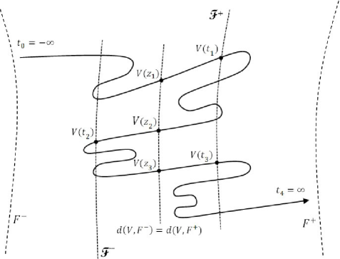
Figure 1. The sequence $-\infty=t_{0}<z_{1}<t_{1}<z_{2}<t_{2}<\ldots<t_{2N}=\infty$, ($N=2$).

Now, let $\{V_{k}\}\subset\mathcal{A}_{b}$ be a minimizing sequence, i.e. $\lim_{k\to\infty}\mathcal{J}_{\mathbb{R}}(V_{k})=\inf_{V\in\mathcal{A}_{b}}\mathcal{J}_{\mathbb{R}}(V)$. For every $k$ we define the sequence

$$-\infty<t_{1}(k)<t_{2}(k)<\ldots<t_{2N_{k}-1}(k)<t_{2N_{k}}(k)=\infty$$

by induction:

• $t_{1}(k)=\sup\{t\in\mathbb{R}:\,V_{k}(s)\in\mathcal{F}^{-},\forall s\leq t\}<\infty$ (note that $V_{k}(t_{1}(k))\in\partial\mathcal{F}^{-}\subset\mathcal{F}^{+}$, and $d(V_{k}(t_{1}(k)),F^{+})<d(V_{k}(t_{1}(k)),F^{-})$, in view of Lemma 2.4 (iv)),

• $t_{2i}(k)=\sup\{t\geq t_{2i-1}(k):\,V_{k}(s)\in\mathcal{F}^{+},\forall s\in[t_{2i-1}(k),t]\}\leq\infty$ (note that $t_{2i}(k)<\infty$ implies that $V_{k}(t_{2i}(k))\in\partial\mathcal{F}^{+}\subset\mathcal{F}^{-}$, and $d(V_{k}(t_{2i}(k)),F^{-})<d(V_{k}(t_{2i}(k)),F^{+})$, in view of Lemma 2.4 (iv)),

• $t_{2i+1}(k)=\sup\{t\geq t_{2i}(k):\,V_{k}(s)\in\mathcal{F}^{-},\forall s\in[t_{2i}(k),t]\}<\infty$, if $t_{2i}(k)<\infty$ (again we have $V_{k}(t_{2i+1}(k))\in\partial\mathcal{F}^{-}\subset\mathcal{F}^{+}$, and $d(V_{k}(t_{2i+1}(k)),F^{+})<d(V_{k}(t_{2i+1}(k)),F^{-})$, in view of Lemma 2.4 (iv)),

where $i=1,\ldots,N_{k}$. In addition, we set

• $z_{2i-1}(k)=\sup\{t\leq t_{2i-1}(k):\,d(V_{k}(t),\mathcal{F}^{-})=d(V_{k}(t),\mathcal{F}^{+})\}$,

• $z_{2i}(k)=\sup\{t\leq t_{2i}(k):\,d(V_{k}(t),\mathcal{F}^{-})=d(V_{k}(t),\mathcal{F}^{+})\}$, if $t_{2i}(k)<\infty$,

and define $b_{j}(k)=\sup\{t\geq z_{j}(k):\|V_{k}(s)-V_{k}(z_{j}(k))\|_{L^{2}(\mathbb{R};\mathbb{R}^{m})}<d_{\mathrm{min}}/4,\forall s\in[z_{j}(k),t]\}$, for $j=1,\ldots,2N_{k}-1$. Since the set $\{v+h:v\in\mathcal{H},\,h\in L^{2}(\mathbb{R};\mathbb{R}^{m}),\,d(v,F^{-})=d(v,F^{+}),\|h\|_{L^{2}(\mathbb{R};\mathbb{R}^{m})}<d_{\mathrm{min}}/4\}$ is included in the interior of $\mathcal{F}^{-}$ (resp. $\mathcal{F}^{+}$), it is clear that $b_{j}(k)\leq t_{j}(k)$. In addition, we have $\inf\{\mathcal{W}(V_{k}(t)):t\in(z_{j}(k),b_{j}(k))\}\geq\mathcal{W}_{0}:=\inf\{\mathcal{W}(v):d(v,F)\geq d_{\mathrm{min}}/4\}>0$, in view of Lemma 2.4 (iv) and Lemma 2.3 (ii). Thus, for every $k\geq 1$ and $j=1,\ldots,2N_{k}-1$, we obtain

$$\mathcal{J}_{(z_{j}(k),b_{j}(k))}(V_{k})\geq\int_{z_{j}(k)}^{b_{j}(k)}\sqrt{2\beta\mathcal{W}(V_{k}(t))}\|V^{\prime}_{k}(t)\|_{L^{2}(\mathbb{R};\mathbb{R}^{m})}\mathrm{d}t\geq\sqrt{2\beta\mathcal{W}_{0}}(d_{\mathrm{min}}/4).$$

This implies that $(2N_{k}-1)\sqrt{2\beta\mathcal{W}_{0}}(d_{\mathrm{min}}/4)\leq\mathcal{J}_{0}$, i.e. the integers $N_{k}$ are uniformly bounded. By passing to a subsequence, we may assume that $N_{k}$ is a constant integer $N\geq 1$.

Our next claim (cf. [24, Lemma 2.4.]) is that up to subsequence, there exist an integer $i_{0}$ ($1\leq i_{0}\leq N$) and an integer $j_{0}$ ($i_{0}\leq j_{0}\leq N$) such that

• the sequence $t_{2j_{0}-1}(k)-t_{2i_{0}-1}(k)$ is bounded,

• $\lim_{k\to\infty}(t_{2i_{0}-1}(k)-t_{2i_{0}-2}(k))=\infty$,

• $\lim_{k\to\infty}(t_{2j_{0}}(k)-t_{2j_{0}-1}(k))=\infty$,

where for convenience we have set $t_{0}(k):=-\infty$. Indeed, we are going to prove by induction on $N\geq 1$, that given $2N+1$ sequences $-\infty\leq t_{0}(k)<t_{1}(k)<\ldots<t_{2N}(k)\leq\infty$, such that $\lim_{k\to\infty}(t_{1}(k)-t_{0}(k))=\infty$, and $\lim_{k\to\infty}(t_{2N}(k)-t_{2N-1}(k))=\infty$, then up to subsequence the properties (a), (b), and (c) above hold, for two fixed indices $1\leq i_{0}\leq j_{0}\leq N$. When $N=1$, the assumption holds by taking $i_{0}=j_{0}=1$. Assume now that $N>1$, and let $l\geq 1$ be the largest integer such that the sequence $t_{l}(k)-t_{1}(k)$ is bounded. Note that $l<2N$. If $l$ is odd, we are done, since the sequence $t_{l+1}(k)-t_{l}(k)$ is unbounded, and thus we can extract a subsequence $\{n_{k}\}$ such that $\lim_{k\to\infty}(t_{l+1}(n_{k})-t_{l}(n_{k}))=\infty$. Otherwise $l=2m$ (with $1\leq m<N$), and the sequence $t_{2m+1}(k)-t_{2m}(k)$ is unbounded. We extract a subsequence $\{n_{k}\}$ such that $\lim_{k\to\infty}(t_{2m+1}(n_{k})-t_{2m}(n_{k}))=\infty$. Then, we apply the inductive statement with $N^{\prime}=N-m$, to the $2N^{\prime}+1$ sequences $t_{2m}(n_{k})<t_{2m+1}(n_{k})<\ldots<t_{2N}(n_{k})$.

To show the existence of the minimizer $U$, we shall consider appropriate translations of the sequence $v_{k}(t,x):=[V_{k}(t)](x)$ ($\mathbb{R}\ni t\mapsto V_{k}(t)\in\mathcal{H}$), with respect to both variables $x$ and $t$. Then, we shall establish the convergence of the translated maps to the minimizer $U$. Given $T\in\mathbb{R}$, and $V\in\mathcal{H}=\operatorname{{\bf e}}_{0}+L^{2}(\mathbb{R};\mathbb{R}^{m})$, we denote by $L^{T}(V)$ the map of $\mathcal{H}$ defined by $\mathbb{R}\ni x\mapsto V(x-T)\in\mathbb{R}^{m}$. It is obvious that $\mathcal{W}(L^{T}(V))=\mathcal{W}(V)$. Similarly, if $t\mapsto V(t)$ belongs to $H^{2}_{\mathrm{loc}}(\mathbb{R};\mathcal{H})$, we obtain that $t\mapsto L^{T}(V(t))$ also belongs to $H^{2}_{\mathrm{loc}}(\mathbb{R};\mathcal{H})$, with

• $(L^{T}V)^{\prime}=L^{T}(V^{\prime})$, $\sigma((L^{T}V)^{\prime})=\sigma(V^{\prime})$, and $\|(L^{T}V)^{\prime}(t)\|_{L^{2}(\mathbb{R};\mathbb{R}^{m})}=\|V^{\prime}(t)\|_{L^{2}(\mathbb{R};\mathbb{R}^{m})}$,

• $(L^{T}V)^{\prime\prime}=L^{T}(V^{\prime\prime})$, and $\|(L^{T}V)^{\prime\prime}(t)\|_{L^{2}(\mathbb{R};\mathbb{R}^{m})}=\|V^{\prime\prime}(t)\|_{L^{2}(\mathbb{R};\mathbb{R}^{m})}$.

At this stage, we infer that the sequence $d(V_{k}(t_{2i_{0}-1}(k)),F^{-})$ is bounded. Indeed, when $k$ is large enough, we have $V_{k}([t_{2i_{0}-1}(k)-\frac{2\mathcal{J}_{0}}{\mathcal{W}_{0}},t_{2i_{0}-1}(k)])\subset\mathcal{F}^{-}$ (where $\mathcal{W}_{0}:=\inf\{\mathcal{W}(v):d(v,F)\geq d_{\mathrm{min}}/4\}>0$). Thus, there exists $s_{k}\in[t_{2i_{0}-1}(k)-\frac{2\mathcal{J}_{0}}{\mathcal{W}_{0}},t_{2i_{0}-1}(k)]$ such that $d(V_{k}(s_{k}),F^{-})<d_{\mathrm{min}}/4$, since otherwise we would obtain $\int_{t_{2i_{0}-1}(k)-\frac{2\mathcal{J}_{0}}{\mathcal{W}_{0}}}^{t_{2i_{0}-1}(k)}\mathcal{W}(V_{k}(t))\mathrm{d}t\geq 2\mathcal{J}_{0}$, which is a contradiction. This proves that $d(V_{k}(t_{2i_{0}-1}(k)),F^{-})\leq d_{\mathrm{min}}/4+d(V_{k}(s_{k}),V_{k}(t_{2i_{0}-1}(k)))\leq\eta:=d_{\mathrm{min}}/4+M\sqrt{\frac{2\mathcal{J}_{0}}{\mathcal{W}_{0}}}$. We also claim that the sets $\mathcal{F}^{\pm}$ are invariant by the translations $L^{T}$. To check this, let us pick $u\in\mathcal{F}^{-}$ (the proof is similar for $\mathcal{F}^{+}$). By definition, $u=v+h$, with $v\in\mathcal{H}$, $h\in L^{2}(\mathbb{R};\mathbb{R}^{m})$, $d(v,F^{-})\leq d(v,F^{+})$, and $\|h\|_{L^{2}(\mathbb{R};\mathbb{R}^{m})}\leq d_{\mathrm{min}}/4$. If $d(v,F^{\pm})=d(v,e^{\pm})$, for some $e^{\pm}\in F^{\pm}$, one can see that $d(L^{T}v,F^{\pm})=d(L^{T}v,L^{T}e^{\pm})=d(v,e^{\pm})$. Therefore, we have $L^{T}u=L^{T}v+L^{T}h$, with $d(L^{T}v,F^{-})\leq d(L^{T}v,F^{+})$, and $\|L^{T}h\|_{L^{2}(\mathbb{R};\mathbb{R}^{m})}=\|h\|_{L^{2}(\mathbb{R};\mathbb{R}^{m})}\leq d_{\mathrm{min}}/4$, i.e. $L^{T}u\in\mathcal{F}^{-}$.

Next, in view of Lemma 2.4 (ii), for every $k$, we can find $T_{k}\in\mathbb{R}$ and $e_{k}\in F^{-}$ such that $\|e_{k}\|_{\mathcal{H}}\leq\gamma$ and $\||L^{T_{k}}V_{k}(t_{2i_{0}-1}(k))-e_{k}\|_{\mathcal{H}}\leq\eta$. We set $\bar{V}_{k}(t):=L^{T_{k}}(V_{k}(t+t_{2i_{0}-1}(k)))$. Clearly, $\bar{V}_{k}\in H^{2}_{\mathrm{loc}}(\mathbb{R};\mathcal{H})$ satisfies $\mathcal{J}_{\mathbb{R}}(\bar{V}_{k})=\mathcal{J}_{\mathbb{R}}(V_{k})$, as well as

(32) $$\bar{V}_{k}(t)\in\mathcal{F}^{-},\forall t\in[t_{2i_{0}-2}(k)-t_{2i_{0}-1}(k),0],\text{ and }\bar{V}_{k}(t)\in\mathcal{F}^{+},\forall t\in[t_{2j_{0}-1}(k)-t_{2i_{0}-1}(k),t_{2j_{0}}(k)-t_{2i_{0}-1}(k)].$$

On the one hand, since $\|\bar{V}_{k}(0)\|_{\mathcal{H}}\leq\eta+\gamma$ holds for every $k$, we have that (up to subsequence) $\bar{V}_{k}(0)\rightharpoonup u_{0}$ in $\mathcal{H}$, as $k\to\infty$, for some $u_{0}\in\mathcal{H}$. On the other hand, since $\bar{V}^{\prime}_{k}$ as well as $\bar{V}^{\prime\prime}_{k}$ are uniformly bounded in $L^{2}(\mathbb{R};L^{2}(\mathbb{R};\mathbb{R}^{m}))$, it follows that up to subsequence

(33) $$\bar{V}^{\prime}_{k}\rightharpoonup U_{1},\text{ and }\bar{V}^{\prime\prime}_{k}\rightharpoonup U_{2}\text{ hold in }L^{2}(\mathbb{R},L^{2}(\mathbb{R};\mathbb{R}^{m})),$$

for some $U_{1},U_{2}\in L^{2}(\mathbb{R};L^{2}(\mathbb{R};\mathbb{R}^{m}))$, such that $U_{1}^{\prime}=U_{2}$, and

(34a) $$\int_{\mathbb{R}}\|U_{1}(t)\|^{2}_{L^{2}(\mathbb{R};\mathbb{R}^{m})}\mathrm{d}t\leq\liminf_{k\to\infty}\int_{\mathbb{R}}\|\bar{V}^{\prime}_{k}(t)\|^{2}_{L^{2}(\mathbb{R};\mathbb{R}^{m})}\mathrm{d}t,$$

(34b) $$\int_{\mathbb{R}}\|U_{2}(t)\|^{2}_{L^{2}(\mathbb{R};\mathbb{R}^{m})}\mathrm{d}t\leq\liminf_{k\to\infty}\int_{\mathbb{R}}\|\bar{V}^{\prime\prime}_{k}(t)\|^{2}_{L^{2}(\mathbb{R};\mathbb{R}^{m})}\mathrm{d}t.$$

Finally, we write $\bar{V}_{k}(t)=\bar{V}_{k}(0)+\int_{0}^{t}\bar{V}^{\prime}_{k}(s)\mathrm{d}s$, and claim that $U(t):=u_{0}+\int_{0}^{t}U_{1}(s)\mathrm{d}s$ is a minimizer of $\mathcal{J}$ in $\mathcal{A}$. Indeed, it is clear that $U\in H^{2}_{\mathrm{loc}}(\mathbb{R};\mathcal{H})$, and since $\int_{0}^{t}\bar{V}^{\prime}_{k}(s)\mathrm{d}s\rightharpoonup\int_{0}^{t}U_{1}(s)\mathrm{d}s$ holds in $\mathcal{H}$ for every $t\in\mathbb{R}$, we also have $\bar{V}_{k}(t)\rightharpoonup U(t)$ for every $t\in\mathbb{R}$. Similarly, since $\|V^{\prime}_{k}(0)\|_{L^{2}(\mathbb{R};\mathbb{R}^{m})}$ is uniformly bounded (cf. Lemma 2.5), it follows that (up to subsequence) $\bar{V}^{\prime}_{k}(0)\rightharpoonup u_{1}$ in $L^{2}(\mathbb{R};\mathbb{R}^{m})$. Thus, for every $t\in\mathbb{R}$, we have $\bar{V}^{\prime}_{k}(t)=\bar{V}^{\prime}_{k}(0)+\int_{0}^{t}\bar{V}^{\prime}_{k}(s)\mathrm{d}s\rightharpoonup u_{1}+\int_{0}^{t}U_{2}(s)\mathrm{d}s=U_{1}(t)+h$, for some $h\in L^{2}(\mathbb{R};\mathbb{R}^{m})$, that we are going to determine. On the one hand, in view of the bound $\|V^{\prime}_{k}(t)\|_{L^{2}(\mathbb{R};\mathbb{R}^{m})}\leq M^{\prime}$, $\forall k$, $\forall t\in\mathbb{R}$, we obtain by dominated convergence that $\lim_{k\to\infty}\int_{0}^{t}\langle\bar{V}^{\prime}_{k}(s),h\rangle_{L^{2}(\mathbb{R};\mathbb{R}^{m})}\mathrm{d}s=\int_{0}^{t}\langle U_{1}(s),h\rangle_{L^{2}(\mathbb{R};\mathbb{R}^{m})}\mathrm{d}s+t\|h\|^{2}_{L^{2}(\mathbb{R};\mathbb{R}^{m})}$. On the other hand, using the weak convergence $\bar{V}^{\prime}_{k}\rightharpoonup U_{1}$ in $L^{2}(\mathbb{R};L^{2}(\mathbb{R};\mathbb{R}^{m}))$, we deduce that $\lim_{k\to\infty}\int_{0}^{t}\langle\bar{V}^{\prime}_{k}(s),h\rangle_{L^{2}(\mathbb{R};\mathbb{R}^{m})}\mathrm{d}s=\int_{0}^{t}\langle U_{1}(s),h\rangle_{L^{2}(\mathbb{R};\mathbb{R}^{m})}\mathrm{d}s$. Thus $h=0$, and we have established that $\bar{V}^{\prime}_{k}(t)\rightharpoonup U_{1}(t)$ holds for every $t\in\mathbb{R}$. Now, the sequentially weakly lower semicontinuity of $\mathcal{W}$ and $\sigma$ (cf. Lemma 2.3 (i)), implies that $\liminf_{k\to\infty}[\sigma(\bar{V}^{\prime}_{k}(t))+\mathcal{W}(\bar{V}_{k}(t))]\geq[\sigma(U_{1}(t))+\mathcal{W}(U(t))]$ for every $t\in\mathbb{R}$, thus by Fatou’s Lemma we obtain

(35) $$\int_{\mathbb{R}}[\sigma(U_{1}(t))+\mathcal{W}(U(t))]\mathrm{d}t\leq\liminf_{k\to\infty}\int_{\mathbb{R}}[\sigma(\bar{V}^{\prime}_{k}(t))+\mathcal{W}(\bar{V}_{k}(t))]\mathrm{d}t.$$

Combining (33) with (34) it is clear that $\mathcal{J}_{\mathbb{R}}(U)\leq\liminf_{k\to\infty}\mathcal{J}_{\mathbb{R}}(V_{k})$. To conclude it remains to show that $U\in\mathcal{A}$. In view of the above property (b) it follows that $U(t)\in\mathcal{F}^{-}$, for every $t\leq 0$. Similarly, in view of (a) and (c), we have $U(t)\in\mathcal{F}^{+}$, for $t\geq T>0$ large enough. ∎

Existence of the double layered solution.

We first identify $U$ with a map $u\in H^{2}_{\mathrm{loc}}(\mathbb{R}^{2};\mathbb{R}^{m})$:

Lemma 3.2.

Writing $U(t)=\operatorname{{\bf e}}_{0}+H(t)$, with

$$H\in H^{2}_{\mathrm{loc}}(\mathbb{R};L^{2}(\mathbb{R};\mathbb{R}^{m}))\subset L^{2}_{\mathrm{loc}}(\mathbb{R};L^{2}(\mathbb{R};\mathbb{R}^{m})),$$

and identifying $H$ with a $L^{2}_{\mathrm{loc}}(\mathbb{R}^{2};\mathbb{R}^{m})$ map via $h(t,x):=[H(t)](x)$, we have

• $h\in H^{2}_{\mathrm{loc}}(\mathbb{R}^{2};\mathbb{R}^{m})$, $h_{t},h_{tt},h_{tx}\in L^{2}(\mathbb{R}^{2};\mathbb{R}^{m})$, and $h_{x},h_{xx}\in L^{2}((t_{1},t_{2})\times\mathbb{R};\mathbb{R}^{m})$ for every interval $[t_{1},t_{2}]\subset\mathbb{R}$.

• Moreover, $\|h_{x}\|_{L^{2}((t_{1},t_{2})\times\mathbb{R};\mathbb{R}^{m})}^{2}+\|h_{xx}\|_{L^{2}((t_{1},t_{2})\times\mathbb{R};\mathbb{R}^{m})}^{2}\leq C_{0}(|t_{2}-t_{1}|)$, for a constant $C_{0}>0$ depending only on $|t_{2}-t_{1}|$.

Proof.

We recall that given any interval $(t_{1},t_{2})$, we can identify $L^{2}((t_{1},t_{2})\times\mathbb{R};\mathbb{R}^{m})$ with $L^{2}((t_{1},t_{2});L^{2}(\mathbb{R};\mathbb{R}^{m}))$ via the canonical isomorphism

$$L^{2}((t_{1},t_{2})\times\mathbb{R};\mathbb{R}^{m}) \simeq L^{2}((t_{1},t_{2});L^{2}(\mathbb{R};\mathbb{R}^{m}))$$

$$f \simeq[(t_{1},t_{2})\ni t\mapsto[F(t)]:x\mapsto f(t,x)],\ F(t)\in L^{2}(\mathbb{R};\mathbb{R}^{m}).$$

Let $g_{1}(t,x):=[U^{\prime}(t)](x)$, $g_{2}(t,x):=[U^{\prime\prime}(t)](x)$, with $g_{1},g_{2}\in L^{2}(\mathbb{R}^{2};\mathbb{R}^{m})$, and let us prove that $h_{t}=g_{1}$. Given a function $\phi\in C^{\infty}_{0}(\mathbb{R}^{2};\mathbb{R}^{m})$, we also view it as a map $\Phi\in C^{1}(\mathbb{R};L^{2}(\mathbb{R};\mathbb{R}^{m}))$, $t\mapsto\Phi(t)$, by setting $[\Phi(t)](x):=\phi(t,x)$. Assuming that $\operatorname{supp}\Phi\subset(t_{1},t_{2})$, we have

$$\int_{\mathbb{R}^{2}}[h\cdot\phi_{t}+g_{1}\cdot\phi]=\int_{t_{1}}^{t_{2}}(\langle H(t),\Phi_{t}(t)\rangle_{L^{2}(\mathbb{R};\mathbb{R}^{m})}+\langle H_{t}(t),\Phi(t)\rangle_{L^{2}(\mathbb{R};\mathbb{R}^{m})})\mathrm{d}t,$$

and clearly the second integral vanishes if $H\in C^{1}([t_{1},t_{2}];L^{2}(\mathbb{R};\mathbb{R}^{m}))$. Since $H$ can be approximated in $H^{1}((t_{1},t_{2});L^{2}(\mathbb{R};\mathbb{R}^{m}))$ by $C^{1}([t_{1},t_{2}];L^{2}(\mathbb{R};\mathbb{R}^{m}))$ maps, we deduce that $\int_{\mathbb{R}^{2}}[h\cdot\phi_{t}+g_{1}\cdot\phi]=0$, i.e. $h_{t}=g_{1}$. Similarly, we can prove that $h_{tt}=\frac{\partial g_{1}}{\partial t}=g_{2}$. On the other hand, to establish that $h_{tx}\in L^{2}(\mathbb{R}^{2};\mathbb{R}^{m})$, we use difference quotients. Indeed, for a.e. $t\in\mathbb{R}$, and for every $\xi\in(-1,1)$, we have

(36) $$\int_{\mathbb{R}}\Big{|}\frac{g_{1}(t,x+\xi)-g_{1}(t,x)}{\xi}\Big{|}^{2}\mathrm{d}x\leq\sigma(g_{1}(t,\cdot))=\sigma(U^{\prime}(t))<\infty,$$

thus after an integration, we obtain

(37) $$\int_{\mathbb{R}^{2}}\Big{|}\frac{g_{1}(t,x+\xi)-g_{1}(t,x)}{\xi}\Big{|}^{2}\mathrm{d}t\mathrm{d}x\leq\int_{\mathbb{R}}\sigma(U^{\prime}(t))\mathrm{d}t<\infty\Rightarrow h_{tx}\in L^{2}(\mathbb{R}^{2};\mathbb{R}^{m}).$$

Finally, since $\int_{\mathbb{R}}\mathcal{W}(U(t))\mathrm{d}t<\infty$ it follows that for a.e. $t\in\mathbb{R}$, we have $\mathcal{W}(U(t))<\infty$, and $U(t)\in\operatorname{{\bf e}}_{0}+H^{2}(\mathbb{R};\mathbb{R}^{m})$. By using again difference quotients, we can see that

(38) $$\int_{\mathbb{R}}\Big{|}\frac{h(t,x+\xi)-h(t,x)}{\xi}\Big{|}^{2}\mathrm{d}x\leq\int_{\mathbb{R}}|h_{x}|^{2}\leq\frac{4(\mathcal{W}(U(t))+J_{\mathrm{min}})}{\beta}+2\|\operatorname{{\bf e}}^{\prime}_{0}\|_{L^{2}(\mathbb{R};\mathbb{R}^{m})}^{2},$$

holds for a.e. $t\in\mathbb{R}$, and for $\xi\in(-1,1)$. As a consequence, the difference quotients $\frac{h(t,x+\xi)-h(t,x)}{\xi}$ (with $\xi\in(-1,1)$) are bounded in $L^{2}((t_{1},t_{2})\times\mathbb{R};\mathbb{R}^{m})$ for every interval $[t_{1},t_{2}]\subset\mathbb{R}$, since an integration of (38) gives

(39) $$\int_{t_{1}}^{t_{2}}\int_{\mathbb{R}}\Big{|}\frac{h(t,x+\xi)-h(t,x)}{\xi}\Big{|}^{2}\mathrm{d}t\mathrm{d}x\leq\frac{4\int_{\mathbb{R}}\mathcal{W}(U(t))\mathrm{d}t}{\beta}+\Big{(}\frac{4J_{\mathrm{min}}}{\beta}+2\|\operatorname{{\bf e}}^{\prime}_{0}\|_{L^{2}(\mathbb{R};\mathbb{R}^{m})}^{2}\Big{)}(t_{2}-t_{1})=:C_{1}(|t_{2}-t_{1}|).$$

This implies that $h_{x}\in L^{2}((t_{1},t_{2})\times\mathbb{R};\mathbb{R}^{m})$, and $\|h_{x}\|^{2}_{L^{2}((t_{1},t_{2})\times\mathbb{R};\mathbb{R}^{m})}\leq C_{1}(|t_{2}-t_{1}|)$. The proof that $h_{xx}\in L^{2}((t_{1},t_{2})\times\mathbb{R};\mathbb{R}^{m})$, with $\|h_{xx}\|^{2}_{L^{2}((t_{1},t_{2})\times\mathbb{R};\mathbb{R}^{m})}\leq C_{2}(|t_{2}-t_{1}|):=4\int_{\mathbb{R}}\mathcal{W}(U(t))\mathrm{d}t+\big{(}4J_{\mathrm{min}}+2\|\operatorname{{\bf e}}^{\prime}_{0}\|_{L^{2}(\mathbb{R};\mathbb{R}^{m})}^{2}\Big{)}(t_{2}-t_{1})$ is similar. ∎

Next, we shall establish that the map $u(t,x):=[U(t)](x)$ is a weak solution of (1). Given a function $\phi\in C^{1}_{0}(\mathbb{R}^{2};\mathbb{R}^{m})$, we also view it as a map $\Phi\in C^{1}_{0}(\mathbb{R};L^{2}(\mathbb{R};\mathbb{R}^{m}))$, $t\mapsto\Phi(t)$, by setting $[\Phi(t)](x):=\phi(t,x)$. For every $\lambda\in\mathbb{R}$, it is clear that

(40) $$\mathcal{J}_{\mathbb{R}}(U)\leq\mathcal{J}_{\mathbb{R}}(U+\lambda\Phi),$$

and

(41a) $$\frac{\mathrm{d}}{\mathrm{d}\lambda}\Big{|}_{\lambda=0}\int_{\mathbb{R}}\frac{1}{2}\|U^{\prime}(t)+\lambda\Phi^{\prime}(t)\|_{L^{2}(\mathbb{R};\mathbb{R}^{m})}^{2}\mathrm{d}t=\int_{\mathbb{R}}\langle U^{\prime}(t),\Phi^{\prime}(t)\rangle_{L^{2}(\mathbb{R};\mathbb{R}^{m})}\mathrm{d}t,$$

(41b) $$\frac{\mathrm{d}}{\mathrm{d}\lambda}\Big{|}_{\lambda=0}\int_{\mathbb{R}}\frac{1}{2}\|U^{\prime\prime}(t)+\lambda\Phi^{\prime\prime}(t)\|_{L^{2}(\mathbb{R};\mathbb{R}^{m})}^{2}\mathrm{d}t=\int_{\mathbb{R}}\langle U^{\prime\prime}(t),\Phi^{\prime\prime}(t)\rangle_{L^{2}(\mathbb{R};\mathbb{R}^{m})}\mathrm{d}t.$$

On the other hand, since $\int_{\mathbb{R}}[\sigma(U^{\prime}(t))+\mathcal{W}(U(t))]\mathrm{d}t<\infty$, it follows that for a.e. $t\in\mathbb{R}$, we have $\sigma(U^{\prime}(t))+\mathcal{W}(U(t))<\infty$, and $U(t)\in\operatorname{{\bf e}}_{0}+H^{2}(\mathbb{R};\mathbb{R}^{m})$ as well as $U^{\prime}(t)\in H^{1}(\mathbb{R};\mathbb{R}^{m})$. Our claim is that

(42) $$\frac{\mathrm{d}}{\mathrm{d}\lambda}\Big{|}_{\lambda=0}\int_{\mathbb{R}}[\sigma(U^{\prime}(t)+\lambda\Phi^{\prime}(t))+\mathcal{W}(U(t)+\lambda\Phi(t))]\mathrm{d}t=\int_{\mathbb{R}}\psi(t)\mathrm{d}t,$$

where

$$\psi(t):=\int_{\mathbb{R}}\big{[}2\frac{\mathrm{d}[U^{\prime}(t)]}{\mathrm{d}x}\cdot\frac{\partial^{2}\phi(t,x)}{\partial t\partial x}+\frac{\mathrm{d}^{2}[U(t)]}{\mathrm{d}x^{2}}\cdot\frac{\partial^{2}\phi(t,x)}{\partial x^{2}}+\beta\frac{\mathrm{d}[U(t)]}{\mathrm{d}x}\cdot\frac{\partial\phi(t,x)}{\partial x}+\nabla W([U(t)](x))\cdot\phi(t,x)\big{]}\mathrm{d}x.$$

Indeed, we first notice that for every $\lambda\neq 0$, the functions $\psi_{\lambda}(t):=\frac{1}{\lambda}[\sigma(U^{\prime}(t)+\lambda\Phi^{\prime}(t))+\mathcal{W}(U(t)+\lambda\Phi(t))-\sigma(U^{\prime}(t))-\mathcal{W}(U(t))]$ are defined a.e. Moreover, we can see that $\psi_{\lambda}(t)$ is equal to

$$\int_{\mathbb{R}}\Big{[}2\frac{\mathrm{d}[U^{\prime}(t)]}{\mathrm{d}x}\cdot\frac{\partial^{2}\phi(t,x)}{\partial t\partial x}+\frac{\mathrm{d}^{2}[U(t)]}{\mathrm{d}x^{2}}\cdot\frac{\partial^{2}\phi(t,x)}{\partial x^{2}}+\beta\frac{\mathrm{d}[U(t)]}{\mathrm{d}x}\cdot\frac{\partial\phi(t,x)}{\partial x}\\ +\lambda\Big{|}\frac{\partial^{2}\phi(t,x)}{\partial t\partial x}\Big{|}^{2}+\frac{\lambda}{2}\Big{|}\frac{\partial^{2}\phi(t,x)}{\partial x^{2}}\Big{|}^{2}+\frac{\beta\lambda}{2}\Big{|}\frac{\partial\phi(t,x)}{\partial x}\Big{|}^{2}+\nabla W([U(t)](x)+c_{\lambda}(t,x)\lambda\phi(t,x))\cdot\phi(t,x)\Big{]}\mathrm{d}x,$$

with $0\leq c_{\lambda}(t,x)\leq 1$. As a consequence, we obtain $\lim_{\lambda\to 0}\psi_{\lambda}(t)=\psi(t)$ for a.e. $t\in\mathbb{R}$. Finally, setting $\kappa=\sup\{|\nabla W(v)|:|v|\leq\|u\|_{L^{\infty}(\operatorname{supp}\phi;\mathbb{R}^{m})}+\|\phi\|_{L^{\infty}(\mathbb{R}^{2};\mathbb{R}^{m})}\}$, there is an integrable function

$$\Psi(t)=\sigma(U^{\prime}(t))+\mathcal{W}(U(t))+\int_{\mathbb{R}}\Big{[}2\Big{|}\frac{\partial^{2}\phi(t,x)}{\partial t\partial x}\Big{|}^{2}+\Big{|}\frac{\partial^{2}\phi(t,x)}{\partial x^{2}}\Big{|}^{2}+\beta\Big{|}\frac{\partial\phi(t,x)}{\partial x}\Big{|}^{2}+\kappa|\phi(t,x)|\Big{]}\mathrm{d}x$$

such that $|\psi_{\lambda}(t)|\leq\Psi(t)$ holds a.e., when $|\lambda|\leq 1$. Thus, we deduce (42) by dominated convergence.

Now, we gather the previous results to conclude. In view of (40), (41) and (42), the minimizer $U$ satisfies the Euler-Lagrange equation

(43) $$\int_{\mathbb{R}}(\langle U^{\prime\prime}(t),\Phi^{\prime\prime}(t)\rangle_{L^{2}(\mathbb{R};\mathbb{R}^{m})}+\beta\langle U^{\prime}(t),\Phi^{\prime}(t)\rangle_{L^{2}(\mathbb{R};\mathbb{R}^{m})}+\psi(t))\mathrm{d}t=0.$$

which is equivalent to

(44) $$\int_{\mathbb{R}^{2}}(\nabla^{2}u\cdot\nabla^{2}\phi+\beta\nabla u\cdot\nabla\phi+\nabla W(u)\cdot\phi)=0.$$

By elliptic regularity, it follows that $u\in C^{4}(\mathbb{R}^{2};\mathbb{R}^{m})$ is a classical solution of (1). On the other hand, it is clear in view of Lemma 3.1 that (15a) holds. Thus to complete the proof of Theorem 1.1, it remains to show (15b). Let us first establish the uniform continuity of $u$ in the strips $[t_{1},t_{2}]\times\mathbb{R}$ (with $[t_{1},t_{2}]\subset\mathbb{R}$). To see this, we shall consider an arbitrary disc $D$ of radius $1$ included in the strip $[t_{1},t_{2}]\times\mathbb{R}$, and check that for such discs, $\|u\|_{H^{2}(D;\mathbb{R}^{m})}$ is uniformly bounded. Indeed, we notice that $\|u\|_{L^{2}(D;\mathbb{R}^{m})}$ is uniformly bounded (independently of $D$), since the function $\mathbb{R}\ni t\mapsto\|u(t,\cdot)-\operatorname{{\bf e}}_{0}(\cdot)\|_{L^{2}(\mathbb{R};\mathbb{R}^{m})}$ is continuous. Next, in view of the $L^{2}$ bounds obtained in Lemma 3.2 for the first and second derivatives of $u$, we deduce our claim. To prove (15b), assume by contradiction the existence of a sequence $(s_{k},x_{k})$ such that $\lim_{k\to\infty}x_{k}=\infty$, $s_{k}\in[t_{1},t_{2}]$, and $|u(s_{k},x_{k})-a^{+}|>\epsilon>0$. As a consequence of the uniform continuity of $u$, we can construct a sequence of disjoint discs of fixed radius, centered at $(s_{k},x_{k})$, over which $W(u)$ is bounded uniformly away from zero. This clearly violates the finiteness of $E_{[t_{1},t_{2}]\times\mathbb{R}}(u)=\mathcal{J}_{[t_{1},t_{2}]}(U)+J_{\mathrm{min}}(t_{2}-t_{1})$. ∎

References

- [1] Alama, S., Bronsard, L., Gui, C.: Stationary layered solutions in for an Allen-Cahn system with multiple well potential. Calc. Var. 5 No. 4, 359–390 (1997)
- [2] Alessio, F.: Stationary layered solutions for a system of Allen-Cahn type equations. Indiana Univ. Math. g. 62, 1535–1564 (2013)
- [3] Alikakos, N. D., Fusco, G.: On the connection problem for potentials with several global minima. Indiana Univ. Math. J. 57, 1871–1906 (2008)
- [4] Antonopoulos, P., Smyrnelis, P.: On minimizers of the Hamiltonian system , and on the existence of heteroclinic, homoclinic and periodic orbits. Indiana Univ. Math. J. 65 No. 5, 1503–1524 (2016)
- [5] Bonheure, D., Sanchez, L.: Heteroclinic orbits for some classes of second and fourth order differential equations. Handbook of differential equations: ordinary differential equations, Vol. III, 103–202, Elsevier/North-Holland, Amsterdam, (2006)
- [6] Bonheure, D., Földes, J., Saldaña: A. Qualitative properties of solutions to mixed-diffusion bistable equations. Calc. Var. 55, 67 (2016)
- [7] Bonheure, D., Hamel, F.: One-dimensional symmetry and Liouville type results for the fourth order Allen-Cahn equation in . Chin. Ann. Math. Ser. B 38, 149–172 (2017)
- [8] Brezis, H.: Opérateurs maximaux monotones et semi-groupes de contractions dans les espaces de Hilbert. 50 in Notas de Matemática. North-Holland Publishing Company (1973)
- [9] Cazenave, T., Haraux, A.: An Introduction to Semilinaer Evolution Equations. Oxford lecture series in mathematics and its applications. Clarendon Press (1998)
- [10] Dee, G. T., van Saarloos, W: Bistable systems with propagating fronts leading to pattern formation. Phys. Rev. Lett. 60, 2641–2644 (1988)
- [11] De Giorgi, E.: Convergence problems for functionals and operators. In: Proceedings of the International Meeting on Recent Methods in Nonlinear Analysis, Rome (1978), 131–188. Pitagora, Bologna (1979)
- [12] Farina, A., Valdinoci, E.: The state of art for a conjecture of De Giorgi and related questions. Reaction-diffusion systems and viscosity solutions. World Scientific, Singapore (2008)
- [13] Fonseca, I., Mantegazza, C.: Second order singular perturbation models for phase transitions. SIAM J. Math. Anal. 31 (2000), 1121–1143.
- [14] Fusco, G.: Layered solutions to the vector Allen-Cahn equation in . Minimizers and heteroclinic connections. Comm. Pure Appl. Anal. 16 No. 5, 1807–1841 (2017)
- [15] Kalies, W. D., Van der Vorst, R. C. A. M.: Multitransition homoclinic and heteroclinic solutions of the extended Fisher-Kolmogorov equation. J. Differential Equations 131 No. 2, 209–228 (1996)
- [16] Gasinski, L., Papageorgiou, N. S.: Nonlinear Analysis. Series in Mathematical Analysis and Applications. CRC Press (2006)
- [17] Hilhorst, D., Peletier, L. A., Schätzle, R.: -limit for the extended Fisher-Kolmogorov equation, Proc. Royal Soc. Edinburgh A 132 (2002), 141–162.
- [18] Kreuter, M.: Sobolev spaces of vector-valued functions. Master thesis, Ulm University, Faculty of Mathematics and Economics (2015)
- [19] Monteil, A., Santambrogio, F.: Metric methods for heteroclinic connections in infinite dimensional spaces. To appear.
- [20] Peletier, L. A., Troy, W. C.: Spatial patterns, higher order models in physics and mechanics. 45, Birkhäuser, Boston, MA (2001)
- [21] Peletier, L. A., Troy, W. C., Van der Vorst, R. C. A. M.: Stationary solutions of a fourth-order nonlinear diffusion equation. Differentsial′nye Uravneniya 31 No. 2, 327–337 (1995)
- [22] Savin, O.: Minimal Surfaces and Minimizers of the Ginzburg Landau energy. Cont. Math. Mech. Analysis AMS 526, 43–58 (2010)
- [23] Schatzman, M.: Asymmetric heteroclinic double layers. Control Optim. Calc. Var. 8 (A tribute to J. L. Lions), 965–1005 (electronic) (2002)
- [24] Smyrnelis, P.: Minimal heteroclinics for a class of fourth order O.D.E. systems. Nonlinear Analysis, Theory, Methods and Applications 173, 154–163 (2018)
- [25] Smyrnelis, P.: Connecting orbits in Hilbert spaces and applicatons to P.D.E. Comm. Pure Appl. Anal. 19, No. 5 (May 2020) 2797–2818, doi: 10.3934/cpaa.2020122