EUROPEAN ORGANIZATION FOR NUCLEAR RESEARCH (CERN)

​​​ CERN-EP-2020-086 LHCb-PAPER-2020-008 March 11, 2021

Study of the lineshape of the ${\chi_{{c}1}}(3872)$ state

LHCb collaboration

A study of the lineshape of the ${\chi_{{c}1}}(3872)$ state is made using a data sample corresponding to an integrated luminosity of $3\mbox{\,fb}^{-1}$ collected in $pp$ collisions at centre-of-mass energies of 7 and 8 TeV with the LHCb detector. Candidate ${\chi_{{c}1}}(3872)$ and ${\psi{(2S)}}$ mesons from ${b}$-hadron decays are selected in the $J/\psi\pi^{+}\pi^{-}$ decay mode. Describing the lineshape with a Breit–Wigner function, the mass splitting between the ${\chi_{{c}1}}(3872)$ and ${\psi{(2S)}}$ states, $\Delta m$, and the width of the ${\chi_{{c}1}}(3872)$ state, $\Gamma_{\mathrm{BW}}$, are determined to be

$$\Delta m = 185.598\pm 0.067\pm 0.068\mathrm{\,Me\kern-1.00006ptV}\,,$$

$$\Gamma_{\mathrm{BW}} = \phantom{00}1.39\phantom{0}\pm 0.24\phantom{0}\pm 0.10\phantom{0}\mathrm{\,Me\kern-1.00006ptV}\,,$$

where the first uncertainty is statistical and the second systematic. Using a Flatté-inspired model, the mode and full width at half maximum of the lineshape are determined to be

$$\mathrm{mode} =3871.69^{\,+\,0.00\,+\,0.05}_{-0.04\,-\,0.13} \mathrm{\,Me\kern-1.00006ptV}$$

$$\mathrm{FWHM} =0.22^{\,+\,0.07\,+\,0.11}_{\,-\,0.06\,-\,0.13} \mathrm{\,Me\kern-1.00006ptV}.$$

An investigation of the analytic structure of the Flatté amplitude reveals a pole structure, which is compatible with a quasi-bound ${{D}^{0}}{{\kern 1.99997pt\overline{\kern-1.99997ptD}{}}{}^{*0}}$ state but a quasi-virtual state is still allowed at the level of $2$ standard deviations.

Published in Phys. Rev. D102 (2020) 092005

© CERN on behalf of the LHCb collaboration, licence CC BY 4.0.

 

1 Introduction

The last two decades have seen a resurgence of interest in the spectroscopy of non-conventional (exotic) charmonium states [1] starting with the observation of the charmonium-like ${\chi_{{c}1}}(3872)$ state by the Belle collaboration [2]. Though the existence of the ${\chi_{{c}1}}(3872)$ particle has been confirmed by many experiments [3, 4, 5, 6, 7] with quantum numbers measured to be $1^{++}$ [8, 9], its nature is still uncertain. Several exotic interpretations have been suggested: e.g. a tetraquark [10], a loosely bound deuteron-like ${{D}^{0}}{{\kern 1.99997pt\overline{\kern-1.99997ptD}{}}{}^{*0}}$ molecule [11] or a charmonium-molecule mixture [12].

A striking feature of the ${\chi_{{c}1}}(3872)$ state is the proximity of its mass to the sum of the ${{D}^{*0}}$ and ${{D}^{0}}$ meson masses. Accounting for correlated uncertainties due to the knowledge of the kaon mass, this sum is evaluated to be $m_{{{D}^{0}}}+m_{{{D}^{*0}}}=3871.70\pm 0.11\mathrm{\,Me\kern-1.00006ptV}$ . The molecular interpretation of the ${\chi_{{c}1}}(3872)$ state requires it to be a bound state. Assuming a Breit–Wigner lineshape, this implies that $\delta E\equiv m_{{{D}^{0}}}+m_{{{D}^{*0}}}-m_{{\chi_{{c}1}}(3872)}>0$. Current knowledge of $\delta E$ is limited by the uncertainty on the ${\chi_{{c}1}}(3872)$ mass, motivating a more precise determination of this quantity. The nature of the ${\chi_{{c}1}}(3872)$ state can also be elucidated by studies of its lineshape. This has been analysed by several experiments assuming a Breit–Wigner function [3, 5, 13]. The current upper limit on the natural width, $\Gamma_{\mathrm{BW}}$, is $1.2\mathrm{\,Me\kern-1.00006ptV}$ at $90\%$ confidence level [14].

In this analysis a sample of ${\chi_{{c}1}}(3872)\rightarrow J/\psi\pi^{+}\pi^{-}$ candidates produced in inclusive ${b}$-hadron decays is used to measure precisely the mass and to determine the lineshape of the ${\chi_{{c}1}}(3872)$ meson. Studies are made assuming both a Breit–Wigner lineshape and a Flatté-inspired model that accounts for the opening up of the ${{\kern 1.99997pt\overline{\kern-1.99997ptD}{}}{}^{0}}{{D}^{*0}}$ threshold [15, 16]. The analysis uses a data sample corresponding to an integrated luminosity of $3\mbox{\,fb}^{-1}$ of data collected in $pp$ collisions at centre-of-mass energies of 7 TeV and 8 TeV during 2011 and 2012 using the LHCb detector.

2 Detector and simulation

The LHCb detector [17, 18] is a single-arm forward spectrometer covering the pseudorapidity range $2<\eta<5$, designed for the study of particles containing $b$ or $c$ quarks. The detector includes a high-precision tracking system consisting of a silicon-strip vertex detector surrounding the $pp$ interaction region [19], a large-area silicon-strip detector (TT) located upstream of a dipole magnet with a bending power of about $4{\mathrm{\,Tm}}$, and three stations of silicon-strip detectors and straw drift tubes [20] placed downstream of the magnet. The tracking system provides a measurement of momentum, $p$, of charged particles with a relative uncertainty that varies from 0.5% at low momentum to 1.0% at 200$\mathrm{\,Ge\kern-1.00006ptV}$. As described in Refs. [21, 22] the momentum scale is calibrated using samples of ${{J\mskip-3.0mu/\mskip-2.0mu\psi\mskip 2.0mu}}\rightarrow{\mu^{+}}{\mu^{-}}$ and ${{B}^{+}}\rightarrow{{J\mskip-3.0mu/\mskip-2.0mu\psi\mskip 2.0mu}}{{K}^{+}}$ decays collected concurrently with the data sample used for this analysis. The relative accuracy of this procedure is estimated to be $3\times 10^{-4}$ using samples of other fully reconstructed ${b}$ hadrons, $\mathchar 28935\relax$ and ${{K}^{0}_{\mathrm{S}}}$ mesons. The minimum distance of a track to a primary vertex (PV), the impact parameter (IP), is measured with a resolution of $(15+29/\mbox{$p_{\mathrm{T}}$}){\,\upmu\mathrm{m}}$, where $p_{\mathrm{T}}$ is the component of the momentum transverse to the beam, in $\mathrm{\,Ge\kern-1.00006ptV}$.

Different types of charged hadrons are distinguished using information from two ring-imaging Cherenkov (RICH) detectors. Photons, electrons and hadrons are identified by a calorimeter system consisting of scintillating-pad and preshower detectors, an electromagnetic calorimeter and a hadronic calorimeter. Muons are identified by a system composed of alternating layers of iron and multiwire proportional chambers [23].

The online event selection is performed by a trigger [24], which consists of a hardware stage, based on information from the calorimeter and muon systems, followed by a software stage, where a full event reconstruction is made. Candidate events are required to pass the hardware trigger, which selects muon and dimuon candidates with high $p_{\mathrm{T}}$ based upon muon system information. The subsequent software trigger is composed of two stages. The first performs a partial event reconstruction and requires events to have two well-identified oppositely charged muons and that the mass of the pair is larger than $2.7\mathrm{\,Ge\kern-1.00006ptV}$. The second stage performs a full event reconstruction. Events are retained for further processing if they contain a displaced ${\mu^{+}}{\mu^{-}}$ vertex. The decay vertex is required to be well separated from each reconstructed PV of the proton-proton interaction by requiring the distance between the PV and the ${\mu^{+}}{\mu^{-}}$ vertex divided by its uncertainty to be greater than three.

To study the properties of the signal and the most important backgrounds, simulated sampels of $pp$ collisions are generated using Pythia [25, *Sjostrand:2007gs] with a specific LHCb configuration [27]. Decays of hadronic particles are described by EvtGen [28], in which final-state radiation is generated using Photos [29]. The interaction of the generated particles with the detector, and its response, are implemented using the Geant4 toolkit [30, *Agostinelli:2002hh] as described in Ref. [32]. For the study of the lineshape it is important that the simulation models well the mass resolution. The simulation used in this study reproduces the observed mass resolution for selected samples of ${{B}^{+}}\rightarrow{{J\mskip-3.0mu/\mskip-2.0mu\psi\mskip 2.0mu}}{{K}^{+}}$, ${{B}^{0}}\rightarrow{{J\mskip-3.0mu/\mskip-2.0mu\psi\mskip 2.0mu}}{{K}^{+}}{{\pi}^{-}}$, ${{B}^{0}_{s}}\rightarrow{{J\mskip-3.0mu/\mskip-2.0mu\psi\mskip 2.0mu}}\phi$ and ${{B}^{+}}\rightarrow{{J\mskip-3.0mu/\mskip-2.0mu\psi\mskip 2.0mu}}{{K}^{+}}{{\pi}^{+}}{{\pi}^{-}}$ decays within $5\%$. To further improve the agreement for the mass resolution between data and simulation, scale factors are determined using a large sample of ${\psi{(2S)}}\rightarrow{{J\mskip-3.0mu/\mskip-2.0mu\psi\mskip 2.0mu}}{{\pi}^{+}}{{\pi}^{-}}$ decays collected concurrently with the ${\chi_{{c}1}}(3872)$ sample. This will be discussed in detail below.

3 Selection

The selection of ${\chi_{{c}1}}(3872)\rightarrow{{J\mskip-3.0mu/\mskip-2.0mu\psi\mskip 2.0mu}}{{\pi}^{+}}{{\pi}^{-}}$ candidates from ${b}$-hadron decays is performed in two steps. First, loose selection criteria are applied that reduce the background from random combinations of tracks significantly while retaining high signal efficiency. Subsequently, a multivariate selection is used to further reduce this combinatorial background. In both steps, the selection requirements are chosen to reduce background whilst selecting well reconstructed candidates. The requirements are optimised using simulated signal decays together with a sample of selected candidates in data where the charged pions have the same sign. The latter sample is found to be a good proxy to describe the background shape. Though the selection criteria are tuned using the ${\chi_{{c}1}}(3872)$ simulation sample, the ${\psi{(2S)}}\rightarrow{{J\mskip-3.0mu/\mskip-2.0mu\psi\mskip 2.0mu}}\pi^{+}\pi^{-}$ decay mode is also selected with high efficiency and used for calibration.

The selection starts from a pair of oppositely charged particles, identified as muons. Incorrectly reconstructed tracks are suppressed by imposing a requirement on the output of a neural network trained to discriminate between these and trajectories from real particles. To select ${{J\mskip-3.0mu/\mskip-2.0mu\psi\mskip 2.0mu}}\rightarrow{\mu^{+}}{\mu^{-}}$ candidates, the two muons are required to originate from a common vertex that is significantly displaced from any PV. The difference between the reconstructed invariant mass of the pair and the known value of the ${{J\mskip-3.0mu/\mskip-2.0mu\psi\mskip 2.0mu}}$ mass [33] is required to be within three times the uncertainty on the reconstructed mass of the ${\mu^{+}}{\mu^{-}}$ pair.

Pion candidates are selected using the same track-quality requirements as the muons. Information from the muon system is used to reject pions that decayed in the spectrometer since these pions tend to have poorly reconstructed trajectories which result in ${\chi_{{c}1}}(3872)$ candidates with worse mass resolution. Combinatorial background is suppressed by requiring that the $\chi^{2}_{\text{IP}}$ of the pion candidates, defined as the difference between the $\chi^{2}$ of the PV reconstructed with and without the considered particle, is larger than four for all PVs. Good pion identification is ensured by applying a requirement on a variable that combines information from the RICH detectors with kinematic and track quality information. Since the pions produced in ${\chi_{{c}1}}(3872)$ decays have relatively small $p_{\mathrm{T}}$, only a loose requirement on the transverse momentum ($\mbox{$p_{\mathrm{T}}$}>200\mathrm{\,Me\kern-1.00006ptV}$) is imposed. In addition, the pion candidates are required to have $p<50\mathrm{\,Ge\kern-1.00006ptV}$. This requirement rejects candidates with poor momentum resolution and has an efficiency of $99.5\,\%$.

To create ${\chi_{{c}1}}(3872)$ candidates, $J/\psi$ candidates are combined with pairs of oppositely charged pions. To improve the mass resolution a kinematic vertex fit [34] is made which constrains the $J/\psi$ invariant mass to its known value [33]. The reduced $\chi^{2}$ of the fit, $\chi^{2}_{\mathrm{fit}}/\mathrm{ndf}$, is required to be less than five. Candidates with a mass uncertainty greater than $5.0\mathrm{\,Me\kern-1.00006ptV}$ are rejected. Finally, requiring the $Q$-value of the decay to be below 200$\mathrm{\,Me\kern-1.00006ptV}$ substantially reduces the background whilst retaining $96\%$ of the ${\chi_{{c}1}}(3872)$ signal. Here the $Q$-value is defined as $Q\equiv m_{{\mu^{+}}{\mu^{-}}{{\pi}^{+}}{{\pi}^{-}}}-m_{{\mu^{+}}{\mu^{-}}}-m_{{{\pi}^{+}}{{\pi}^{-}}}$ where $m_{{\mu^{+}}{\mu^{-}}{{\pi}^{+}}{{\pi}^{-}}}$, $m_{{\mu^{+}}{\mu^{-}}}$ and $m_{{{\pi}^{+}}{{\pi}^{-}}}$ are the reconstructed masses of the final state combinations.

The final step of the selection process is based on a neural network classifier [35, 36, 37, 38, *TMVA4]. This is trained on a simulated sample of inclusive ${b}\rightarrow{\chi_{{c}1}}(3872)X$ decays and the same-sign pion sample in data. Simulated samples are corrected to reproduce kinematical distributions of the $\psi{(2S)}$ mesons observed on data. The training is performed separately for the 2011 and 2012 data samples. Twelve variables that give good separation between signal and background are considered: the pseudorapidity and transverse momentum of the two pion candidates, the $\chi^{2}_{\text{IP}}$ for each of the two pions, the pseudorapidity and transverse momentum of the ${\chi_{{c}1}}(3872)$ candidate, the $\chi^{2}$ of the two-track vertex fit for the pions, the $\chi^{2}_{\mathrm{fit}}/\mathrm{ndf}$, the flight distance $\chi^{2}$ of the candidate calculated using the reconstructed primary and secondary vertices, and the total number of hits in the TT detector. All these variables show good agreement between simulation and data. The optimal cut on the classifier output is chosen using pseudoexperiments so as to minimise the uncertainty on the measured ${\chi_{{c}1}}(3872)$ mass.

4 Mass model

The observed invariant mass distribution of the ${{J\mskip-3.0mu/\mskip-2.0mu\psi\mskip 2.0mu}}{{\pi}^{+}}{{\pi}^{-}}$ system, $m_{{{J\mskip-3.0mu/\mskip-2.0mu\psi\mskip 2.0mu}}{{\pi}^{+}}{{\pi}^{-}}}$, for the ${\psi{(2S)}}$ and ${\chi_{{c}1}}(3872)$ resonances is a convolution of the natural lineshape with the detector resolution. For the ${\psi{(2S)}}$ resonance the lineshape is well described by a Breit–Wigner function. The situation for the ${\chi_{{c}1}}(3872)$ meson is more complex. Previous measurements have assumed a Breit–Wigner resonance shape. However, as discussed in Refs. [15, 16, 12], this is not well motivated due to the proximity of the ${{D}^{0}}{{\kern 1.99997pt\overline{\kern-1.99997ptD}{}}{}^{*0}}$ threshold. Several other alternative lineshapes have been proposed in the literature [15, 16, 40, 41]. In this analysis two lineshapes for the ${\chi_{{c}1}}(3872)$ meson are considered in detail, a Breit–Wigner and a Flatté-inspired model [15, 16]. These models are investigated in the next sections. The S-wave threshold resonance model described in Ref. [40, 41], that accounts for the non-zero width of the $D^{*0}$ meson, was considered but did not fit the data well. If the mass is close to the ${{\kern 1.99997pt\overline{\kern-1.99997ptD}{}}{}^{0}}{{D}^{*0}}$ threshold, this model is not able to accommodate a value of the natural width much larger than $\Gamma_{{{D}^{*0}}}=65.5\pm 15.4\mathrm{\,ke\kern-1.00006ptV}$ [40]. As will be discussed below, the study presented here favours larger values of the natural width.

The analysis proceeds in two steps. First, unbinned maximum-likelihood fits are made to the $m_{{{J\mskip-3.0mu/\mskip-2.0mu\psi\mskip 2.0mu}}{{\pi}^{+}}{{\pi}^{-}}}$ distribution in the region around the ${\psi{(2S)}}$ mass. These measured values of the ${\psi{(2S)}}$ mass and mass resolution are used to control systematic uncertainties in the subsequent fits to the $m_{{{J\mskip-3.0mu/\mskip-2.0mu\psi\mskip 2.0mu}}{{\pi}^{+}}{{\pi}^{-}}}$ distribution in the ${\chi_{{c}1}}(3872)$ mass region. For both sets of fits the natural lineshape is convolved with a resolution model developed using the simulation. The application of the ${{J\mskip-3.0mu/\mskip-2.0mu\psi\mskip 2.0mu}}$ mass constraint in the fit [34] results in the mass resolution being dominated by the kinematics of the pion pair. In particular, the resolution is worse for higher values of the total momentum of the pion pair, $p_{{{\pi}^{+}}{{\pi}^{-}}}$. Consequently, the analysis is performed in three $p_{{{\pi}^{+}}{{\pi}^{-}}}$ bins chosen to contain an approximately equal number of signal candidates: $p_{{{\pi}^{+}}{{\pi}^{-}}}<12\mathrm{\,Ge\kern-1.00006ptV}$, $12\leq p_{{{\pi}^{+}}{{\pi}^{-}}}<20\mathrm{\,Ge\kern-1.00006ptV}$ and $20\leq p_{{{\pi}^{+}}{{\pi}^{-}}}<50\mathrm{\,Ge\kern-1.00006ptV}$. The core mass resolution for the ${\chi_{{c}1}}(3872)$ state varies monotonically between $2.4\mathrm{\,Me\kern-1.00006ptV}$ and $3.0\mathrm{\,Me\kern-1.00006ptV}$ between the lowest-$p_{{{\pi}^{+}}{{\pi}^{-}}}$ and highest-$p_{{{\pi}^{+}}{{\pi}^{-}}}$ bin. Possible differences in data taking conditions are allowed for by dividing the data according to the year of collection resulting in a total of six data samples.

The resolution model is studied using simulation. In each $p_{{{\pi}^{+}}{{\pi}^{-}}}$ bin the mass resolution is modelled with the sum of a narrow Crystal Ball function [42] combined with a wider Gaussian function. The Crystal Ball function has a Gaussian core and two parameters that describe the power-law tail. The simulation is also used to determine the value of the transition point between the core and the power law tail, $a$, as a multiple of the width, $\sigma$, of the Gaussian core. The value of the exponent of the power law, $n$, is allowed to vary in the data fits with a Gaussian constraint to the value obtained in the simulation applied. When fitting the ${\chi_{{c}1}}(3872)$ mass region in data the values of the core resolution, $\sigma$, for the Gaussian and Crystal Ball functions are taken from simulation up to an overall scale factor, $s_{f}$, that accounts for residual discrepancies between data and simulation. For each $p_{{{\pi}^{+}}{{\pi}^{-}}}$ data sample the value of $s_{f}$ is determined in the corresponding fit to the ${\psi{(2S)}}$ mass region and applied as a Gaussian constraint. The systematic uncertainty associated with the choice of the signal model is assessed by replacing the nominal model with the sum of either two Crystal Ball or Gaussian functions.

The shape of the combinatorial background is studied using the same-sign data sample as well as samples of simulated inclusive $b\rightarrow J/\psi X$ decays. Based upon these studies, the background is modelled by the form $(m_{{{J\mskip-3.0mu/\mskip-2.0mu\psi\mskip 2.0mu}}{{\pi}^{+}}{{\pi}^{-}}}-m_{{{J\mskip-3.0mu/\mskip-2.0mu\psi\mskip 2.0mu}}}-2m_{\pi^{\pm}})^{c_{0}}\,e^{-m_{{{J\mskip-3.0mu/\mskip-2.0mu\psi\mskip 2.0mu}}{{\pi}^{+}}{{\pi}^{-}}}/c_{1}}$, where $c_{0}$ is fixed to 3.6 based on fits to the same-sign data. Variations of this functional form together with other models (e.g. exponential or polynomial functions) are used as systematic variations. In total, seven different background forms are considered.

5 $\psi{(2S)}$ mass

Since the $\psi{(2S)}$ state is narrow and away from the phase-space limits, a spin-0 relativistic Breit-Wigner function is used to model the lineshape. A spin-1 Breit-Wigner function is considered as part of the systematic uncertainties and found to give identical results. This lineshape is convolved with the default resolution model and a fit to ${{J\mskip-3.0mu/\mskip-2.0mu\psi\mskip 2.0mu}}{{\pi}^{+}}{{\pi}^{-}}$ mass is performed in each of the six $p_{{{\pi}^{+}}{{\pi}^{-}}}$ data samples. The natural width of the ${\psi{(2S)}}$ is fixed to the known value [33]. Figure 1 shows the $m_{{{J\mskip-3.0mu/\mskip-2.0mu\psi\mskip 2.0mu}}{{\pi}^{+}}{{\pi}^{-}}}$ distributions and fit projections for each data sample and Table 1 summarises the resulting parameters of interest. Binning the data and calculating the $\chi^{2}$ probability of consistency with the fit model gives the values greater than 5% for all fits. The fitted values of the $\psi{(2S)}$ mass agree with the known value [33] within the uncertainty of the calibration procedure. The values of $s_{f}$ are consistent with the expectation that the simulation reproduces the mass resolution in data at the level of $5\%$ or better. When applied as constraint in the fit to the ${\chi_{{c}1}}(3872)$ region, additional uncertainties on $s_{f}$ are considered. Accounting for the finite size of the simulation samples, the background modelling and the assumption that the $\psi(2S)$ calibration factor can be applied to the ${\chi_{{c}1}}(3872)$ candidates, the uncertainty on $s_{f}$ is 0.02, independent of the bin. The values of $s_{f}$ in Table 1 are applied as Gaussian constraints in the fits to the ${\chi_{{c}1}}(3872)$ region with an uncertainty of 0.02.

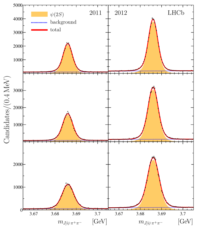
Figure 1: Mass distributions for ${{J\mskip-3.0mu/\mskip-2.0mu\psi\mskip 2.0mu}}{{\pi}^{+}}{{\pi}^{-}}$ candidates in the ${\psi{(2S)}}$ region for (top) the low, (middle) mid and (bottom) high $p_{{{\pi}^{+}}{{\pi}^{-}}}$ bins. The left (right)-hand plot is for 2011 (2012) data. The projection of the fit described in the text is superimposed.

Table 1: Results of the ${\psi{(2S)}}$ mass and scale factor $s_{f}$ obtained for the nominal fit model. The quoted uncertainties on the ${\psi{(2S)}}$ mass and $s_{f}$ are statistical.

Year	$p_{{{\pi}^{+}}{{\pi}^{-}}}~{}\left[\!\mathrm{\,Ge\kern-1.00006ptV}\right]$	$m_{{\psi{(2S)}}}~{}\left[\!\mathrm{\,Me\kern-1.00006ptV}\right]$	$s_{f}$
2011	$\phantom{00\leq}p_{{{\pi}^{+}}{{\pi}^{-}}}<12$	$3685.97\pm 0.02$	$1.03\pm 0.01$
2011	$12\leq p_{{{\pi}^{+}}{{\pi}^{-}}}<20$	$3685.98\pm 0.02$	$1.05\pm 0.01$
2011	$20\leq p_{{{\pi}^{+}}{{\pi}^{-}}}<50$	$3686.10\pm 0.03$	$1.04\pm 0.01$
2012	$\phantom{00\leq}p_{{{\pi}^{+}}{{\pi}^{-}}}<12$	$3686.01\pm 0.01$	$1.03\pm 0.01$
2012	$12\leq p_{{{\pi}^{+}}{{\pi}^{-}}}<20$	$3686.02\pm 0.01$	$1.05\pm 0.01$
2012	$20\leq p_{{{\pi}^{+}}{{\pi}^{-}}}<50$	$3686.09\pm 0.02$	$1.01\pm 0.01$

6 Breit–Wigner mass and width of the ${\chi_{{c}1}}(3872)$ state

To extract the Breit–Wigner lineshape parameters of the ${\chi_{{c}1}}(3872)$ meson, a fit is made to the mass range $3832<m_{{{J\mskip-3.0mu/\mskip-2.0mu\psi\mskip 2.0mu}}{{\pi}^{+}}{{\pi}^{-}}}<3912\mathrm{\,Me\kern-1.00006ptV}$ in each of the six $p_{{{\pi}^{+}}{{\pi}^{-}}}$ data samples described above. A spin-0 relativistic Breit-Wigner is used, as in Ref. [9],

For each data sample the mass difference between the ${\psi{(2S)}}$ and ${\chi_{{c}1}}(3872)$ meson, $\Delta m$, is measured relative to the measured mass of the $\psi{(2S)}$ state rather than the absolute mass. This minimises the systematic uncertainty due to the momentum scale. The fit in each bin has seven free parameters: $\Delta m$, the natural width $\Gamma_{\mathrm{BW}}$, the background parameter $c_{1}$, the resolution scale factor $s_{f}$, the tail parameter $n$, and the signal and background yields. Again a Gaussian constraint is applied to $n$ based on the simulation. The parameter $s_{f}$ is constrained to the result of the fit to the ${\psi{(2S)}}$ data. The fit procedure is validated using both the simulation and pseudoexperiments. No significant bias is found and the uncertainties estimated by the fit agree with the spread observed in the pseudoexperiments. These studies show that, values of $\Gamma_{\mathrm{BW}}$ larger than $0.6\mathrm{\,Me\kern-1.00006ptV}$ can reliably be determined.

For the six $p_{{{\pi}^{+}}{{\pi}^{-}}}$ data samples the ${{J\mskip-3.0mu/\mskip-2.0mu\psi\mskip 2.0mu}}{{\pi}^{+}}{{\pi}^{-}}$ mass distributions in the ${\chi_{{c}1}}(3872)$ region and fits are shown in Fig. 2 and the results summarised in Table 2. Binning the data and calculating the $\chi^{2}$ probability of consistency with the fit model gives values much larger than $5\%$ for all bins apart from the high-momentum bin in the 2012 data where the probability is $2\%$. The values of $\Delta m$ and $\Gamma_{\mathrm{BW}}$ are consistent between the bins giving confidence in the results.

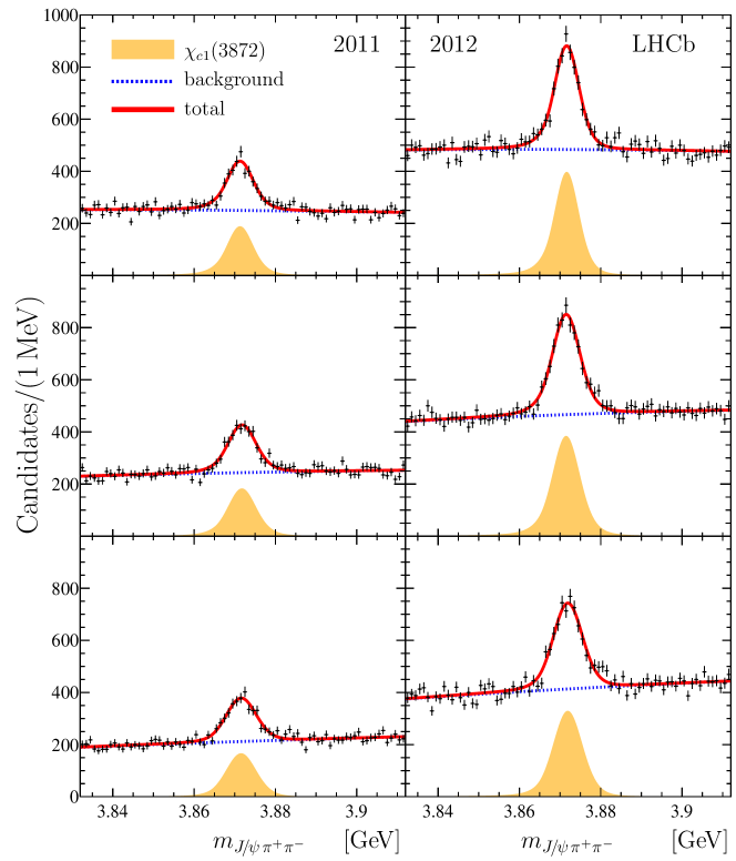
Figure 2: Mass distributions for ${{J\mskip-3.0mu/\mskip-2.0mu\psi\mskip 2.0mu}}{{\pi}^{+}}{{\pi}^{-}}$ candidates in the ${\chi_{{c}1}}(3872)$ region for (top) the low, (middle) mid and (bottom) high $p_{{{\pi}^{+}}{{\pi}^{-}}}$ bins. The left (right)-hand plot is for 2011 (2012) data. The projection of the fit described in the text is superimposed.

Table 2: Results for $\Delta m$ and $\Gamma_{\mathrm{BW}}$ and ${\chi_{{c}1}}(3872)$ signal yields. The quoted uncertainties are statistical.

Year	$p_{{{\pi}^{+}}{{\pi}^{-}}}~{}\left[\!\mathrm{\,Ge\kern-1.00006ptV}\right]$	$\Delta m~{}\left[\!\mathrm{\,Me\kern-1.00006ptV}\right]$	$\Gamma_{\mathrm{BW}}~{}\left[\!\mathrm{\,Me\kern-1.00006ptV}\right]$	$N_{\mathrm{sig}}~{}\left[10^{3}\right]$
2011	$\phantom{00\leq}p_{{{\pi}^{+}}{{\pi}^{-}}}<12$	$185.32\phantom{0}\pm 0.20\phantom{0}$	$1.88\pm 0.74$	$\phantom{0}1.78\pm 0.13$
2011	$12\leq p_{{{\pi}^{+}}{{\pi}^{-}}}<20$	$185.78\phantom{0}\pm 0.21\phantom{0}$	$1.53\pm 0.74$	$\phantom{0}1.79\pm 0.13$
2011	$20\leq p_{{{\pi}^{+}}{{\pi}^{-}}}<50$	$185.46\phantom{0}\pm 0.21\phantom{0}$	$1.03\pm 0.82$	$\phantom{0}1.68\pm 0.13$
2012	$\phantom{00\leq}p_{{{\pi}^{+}}{{\pi}^{-}}}<12$	$185.63\phantom{0}\pm 0.13\phantom{0}$	$1.23\pm 0.47$	$\phantom{0}3.24\pm 0.18$
2012	$12\leq p_{{{\pi}^{+}}{{\pi}^{-}}}<20$	$185.47\phantom{0}\pm 0.14\phantom{0}$	$1.48\pm 0.48$	$\phantom{0}3.70\pm 0.18$
2012	$20\leq p_{{{\pi}^{+}}{{\pi}^{-}}}<50$	$185.81\phantom{0}\pm 0.15\phantom{0}$	$1.15\pm 0.57$	$\phantom{0}3.26\pm 0.17$
Total		$185.588\pm 0.067$	$1.39\pm 0.24$	$15.63\pm 0.38$

A simultaneous fit is made to the six data samples with $\Delta m$ and $\Gamma_{\mathrm{BW}}$ as shared parameters. This gives $\Delta m=185.588\pm 0.067\mathrm{\,Me\kern-1.00006ptV}$ and $\Gamma_{\mathrm{BW}}=1.39\pm 0.24\mathrm{\,Me\kern-1.00006ptV}$, where the uncertainties are statistical. Consistent values are found when these parameters are determined through a weighted average of the six individual bins, or by summing the likelihood profiles returned by the fit.

The dominant systematic uncertainty on the mass difference $\Delta m$ arises from the $3\times 10^{-4}$ relative uncertainty on the momentum scale. Its effect is evaluated by adjusting the four-vectors of the pions by this amount and repeating the analysis. The bias on $\Delta m$ from QED radiative corrections is determined to be $(-10\pm 14)\mathrm{\,ke\kern-1.00006ptV}$ using the simulation, which uses Photos [29] to model this effect. The measured value of $\Delta m$ is corrected by this value and the uncertainty considered as a systematic error. The small uncertainty on the fitted values of the ${\psi{(2S)}}$ mass is also propagated to the $\Delta m$ value. Biases arising from the modelling of the resolution and the treatment of the background shape are evaluated to be $2\mathrm{\,ke\kern-1.00006ptV}$ using the discrete profiling method described in Ref. [43]. The uncertainties on the $\Delta m$ measurement are summarised in Table 3. Combining all uncertainties, the mass splitting between the ${\chi_{{c}1}}(3872)$ and ${\psi{(2S)}}$ mesons is determined as

$$\Delta m=185.598\pm 0.067\pm 0.068\mathrm{\,Me\kern-1.00006ptV}\,,$$

where the first uncertainty is statistical and the second is systematic. The value of $\Delta m$ can be translated into an absolute measurement of the ${\chi_{{c}1}}(3872)$ mass using $m_{{\psi{(2S)}}}=3686.097\pm 0.010\mathrm{\,Me\kern-1.00006ptV}$ from Ref. [33], yielding

$$m_{{\chi_{{c}1}}(3872)}=3871.695\pm 0.067\pm 0.068\pm 0.010\mathrm{\,Me\kern-1.00006ptV}\,,$$

where the third uncertainty is due to the knowledge of the $\psi{(2S)}$ mass. For these measurements it is assumed that interference effects with other partially reconstructed ${b}$-hadron decays do not affect the lineshape. This assumption is reasonable since many exclusive ${b}$-hadron decays contribute to the final sample, and the ${\chi_{{c}1}}(3872)$ state is narrow. This assumption has been explored in pseudoexperiments varying the composition and phases of the possible decay amplitudes that are likely to contribute to the observed data set. These studies conservatively limit the size of any possible effect on $m_{{\chi_{{c}1}}(3872)}$ to be less than $40\mathrm{\,ke\kern-1.00006ptV}$.

Table 3: Systematic uncertainties on the measurement of the mass difference $\Delta m$.

Source	Uncertainty $\left[\!\mathrm{\,Me\kern-1.00006ptV}\right]$
Momentum scale	0.066
Radiative corrections	0.014
Fitted ${\psi{(2S)}}$ mass uncertainty	0.007
Signal + background model	0.002
Sum in quadrature	0.068

The uncertainties from the knowledge of $s_{f}$ and $n$ are already included in the statistical uncertainty of $\Gamma_{\mathrm{BW}}$ via the Gaussian constraints. Their contribution to the statistical uncertainty is estimated to be $0.05\mathrm{\,Me\kern-1.00006ptV}$ by comparison to a fit with these parameters fixed. Further uncertainties arise from the choice of signal and background model. These are evaluated using the discrete profiling method with the alternative models described above. Based upon these studies an uncertainty of $0.10\mathrm{\,Me\kern-1.00006ptV}$ is assigned. The uncertainty due to possible differences in the $p_{\mathrm{T}}$ distribution between data and simulation is evaluated by weighting the simulation to achieve better agreement and lead to a $0.01\mathrm{\,Me\kern-1.00006ptV}$ uncertainty. Summing these values in quadrature gives a total uncertainty of $0.1\mathrm{\,Me\kern-1.00006ptV}$.

The value of $\Gamma_{\mathrm{BW}}$, including systematic uncertainties,

$$\Gamma_{\mathrm{BW}}=1.39\pm 0.24\pm 0.10\mathrm{\,Me\kern-1.00006ptV}\,,$$

differs from zero by more than $5$ standard deviations. Fits were also made fixing $\Gamma_{\mathrm{BW}}$ to zero and allowing $s_{f}$ to float in each bin without constraint. The value of $s_{f}$ obtained is between 1.2 and 1.25 depending on the bin, much larger than can be reasonably explained by differences in the mass resolution between data and simulation after the calibration using the ${\psi{(2S)}}$ data.

Care is needed in the interpretation of the measured $\Gamma_{\mathrm{BW}}$ and $m_{{\chi_{{c}1}}(3872)}$ parameters since $\left|m_{{{D}^{0}}}+m_{{{\kern 1.39998pt\overline{\kern-1.39998ptD}{}}{}^{*0}}}-m_{{\chi_{{c}1}}(3872)}\right|<\Gamma_{\mathrm{BW}}$. The Breit–Wigner parameterisation may not be valid since it neglects the opening of the ${{D}^{0}}{{\kern 1.99997pt\overline{\kern-1.99997ptD}{}}{}^{*0}}$ channel.

7 Flatté model

7.1 The Flatté lineshape model

The proximity of the ${\chi_{{c}1}}(3872)$ mass to the ${D}^{0}$ ${\kern 1.99997pt\overline{\kern-1.99997ptD}{}}{}^{*0}$ threshold distorts the lineshape from the simple Breit–Wigner form. This has to be taken into account explicitly. The general solution to this problem requires a full understanding of the analytic structure of the coupled-channel scattering amplitude. However, if the relevant threshold is close to the resonance, simplified parametrisations are available and have been used to describe the ${\chi_{{c}1}}(3872)$ lineshape [15, 16].

In the ${{J\mskip-3.0mu/\mskip-2.0mu\psi\mskip 2.0mu}}{{\pi}^{+}}{{\pi}^{-}}$ channel the ${\chi_{{c}1}}(3872)$ lineshape as a function of the energy with respect to the ${{D}^{0}}{{\kern 1.99997pt\overline{\kern-1.99997ptD}{}}{}^{*0}}$ threshold, $E\equiv m_{{{J\mskip-3.0mu/\mskip-2.0mu\psi\mskip 2.0mu}}{{\pi}^{+}}{{\pi}^{-}}}-\left(m_{{{D}^{0}}}+m_{{{D}^{*0}}}\right)$, can be written as

$$\dfrac{dR({{J\mskip-3.0mu/\mskip-2.0mu\psi\mskip 2.0mu}}{{\pi}^{+}}{{\pi}^{-}})}{dE}\propto\dfrac{\Gamma_{\rho}(E)}{\left|D(E)\right|^{2}},$$ (1)

where $\Gamma_{\rho}(E)$ is the contribution of the ${{J\mskip-3.0mu/\mskip-2.0mu\psi\mskip 2.0mu}}{{\pi}^{+}}{{\pi}^{-}}$ channel to the width of the ${\chi_{{c}1}}(3872)$ state. The complex-valued denominator function, taking into account the ${{D}^{0}}{{\kern 1.99997pt\overline{\kern-1.99997ptD}{}}{}^{*0}}$ and ${{D}^{+}}{{D}^{*-}}$ two-body thresholds, and the ${{J\mskip-3.0mu/\mskip-2.0mu\psi\mskip 2.0mu}}{{\pi}^{+}}{{\pi}^{-}}$ ${{J\mskip-3.0mu/\mskip-2.0mu\psi\mskip 2.0mu}}{{\pi}^{+}}{{\pi}^{-}}{{\pi}^{0}}$ channels, is given by

$$D(E)=E-E_{f}+\frac{i}{2}\left[g\left(k_{1}+k_{2}\right)+\Gamma_{\rho}(E)+\Gamma_{\omega}(E)+\Gamma_{0}\right].$$ (2)

The Flatté energy parameter, $E_{f}$, is related to a mass parameter, $m_{0}$, via the relation $E_{f}=m_{0}-(m_{{{D}^{0}}}+m_{{{D}^{*0}}})$. The width $\Gamma_{0}$ is introduced in Ref. [16] to represent further open channels, such as radiative decays. The model assumes an isoscalar assignment of the ${\chi_{{c}1}}(3872)$ state, using the same effective coupling, $g$, for both channels. The relative momenta of the decay products in the rest frame of the two-body system, $k_{1}$ for ${{D}^{0}}{{\kern 1.99997pt\overline{\kern-1.99997ptD}{}}{}^{*0}}$ and $k_{2}$ for the ${{D}^{+}}{{D}^{*-}}$ channel, are given by

$$k_{1}=\sqrt{2\mu_{1}E},\ \quad k_{2}=\sqrt{2\mu_{2}(E-\delta)}\,,$$ (3)

where $\delta=8.2\mathrm{\,Me\kern-1.00006ptV}$ is the isospin splitting between the two channels. The reduced masses are given by $\mu_{1}=\tfrac{m_{{{D}^{0}}}m_{{{D}^{*0}}}}{(m_{{{D}^{0}}}+m_{{{D}^{*0}}})}$ and $\mu_{2}=\tfrac{m_{{{D}^{+}}}m_{{{D}^{*-}}}}{(m_{{{D}^{+}}}+m_{{{D}^{*-}}})}$. For $m_{{{J\mskip-3.0mu/\mskip-2.0mu\psi\mskip 2.0mu}}{{\pi}^{+}}{{\pi}^{-}}}$ masses below the ${{D}^{0}}{{\kern 1.99997pt\overline{\kern-1.99997ptD}{}}{}^{*0}}$ and ${{D}^{+}}{{D}^{*-}}$ thresholds these momenta become imaginary and thus their contribution to the denominator will be real. The energy dependence of the ${{J\mskip-3.0mu/\mskip-2.0mu\psi\mskip 2.0mu}}{{\pi}^{+}}{{\pi}^{-}}$ and ${{J\mskip-3.0mu/\mskip-2.0mu\psi\mskip 2.0mu}}{{\pi}^{+}}{{\pi}^{-}}{{\pi}^{0}}$ partial widths is given by [16]

$$\Gamma_{\rho}(E)= f_{\rho}\int\limits_{2m_{\pi}}^{M(E)}\dfrac{dm^{\prime}}{2\pi}\dfrac{q(m^{\prime},E)\,\Gamma_{\rho}}{(m^{\prime}-m_{\rho})^{2}+\Gamma_{\rho}^{2}/4}\,,$$ (4)

$$\Gamma_{\omega}(E)= f_{\omega}\int\limits_{3m_{\pi}}^{M(E)}\dfrac{dm^{\prime}}{2\pi}\dfrac{q(m^{\prime},E)\,\Gamma_{\omega}}{(m^{\prime}-m_{\omega})^{2}+\Gamma_{\omega}^{2}/4}\,.$$ (5)

The known values for masses $m_{\rho}$, $m_{\omega}$ and widths $\Gamma_{\rho}$, $\Gamma_{\omega}$ [33] are used and the lineshapes are approximated with fixed-width Breit–Wigner functions. The partial widths are parameterised by the respective effective couplings $f_{\rho}$ and $f_{\omega}$ and the phase space of these decays, where intermediate resonances $\rho^{0}\!\rightarrow{{\pi}^{+}}{{\pi}^{-}}$ and $\omega\!\rightarrow{{\pi}^{+}}{{\pi}^{-}}{{\pi}^{0}}$ are assumed. The dependence on $E$ is given by the upper boundary of the integrals $M(E)=E+(m_{{{D}^{0}}}+m_{{{D}^{*0}}})-m_{{{J\mskip-3.0mu/\mskip-2.0mu\psi\mskip 2.0mu}}}$. The momentum of the two- or three-pion system in the rest frame of the ${\chi_{{c}1}}(3872)$ is given by

$$q(m^{\prime},E)=\sqrt{\dfrac{\left[M^{2}(E)-(m^{\prime}+m_{{{J\mskip-3.0mu/\mskip-2.0mu\psi\mskip 2.0mu}}})^{2}\right]\left[M^{2}(E)-(m^{\prime}-m_{{{J\mskip-3.0mu/\mskip-2.0mu\psi\mskip 2.0mu}}})^{2}\right]}{4M^{2}(E)}}.$$ (6)

The model as specified contains five free parameters: $m_{0},g,\Gamma_{0}$ and the effective couplings $f_{\rho}$ and $f_{\omega}$. In contrast to the Breit–Wigner lineshape, the parameters of the Flatté model cannot be easily interpreted in terms of the mass and width of the state. Instead it is necessary to determine the location of the poles of the amplitude. The analysis proceeds with a fit of the Flatté amplitude to the data and subsequent search for the poles.

The resulting Flatté lineshape replaces the Breit–Wigner function and is convolved with the resolution models described in the first part of the paper. The Flatté parameters are estimated from a simultaneous unbinned likelihood fit to the ${{J\mskip-3.0mu/\mskip-2.0mu\psi\mskip 2.0mu}}{{\pi}^{+}}{{\pi}^{-}}$ mass distribution in the six $p_{{{\pi}^{+}}{{\pi}^{-}}}$ data samples. The data points are corrected for the observed shifts of the reconstructed mass of the $\psi{(2S)}$ in each bin.

7.2 Fits of the Flatté lineshape to the data

In order to obtain stable results when using the coupled channel model to describe the ${{J\mskip-3.0mu/\mskip-2.0mu\psi\mskip 2.0mu}}{{\pi}^{+}}{{\pi}^{-}}$ mass spectrum, a relation between the effective couplings $f_{\rho}$ and $f_{\omega}$ is imposed. This relation requires that the branching fractions of the ${\chi_{{c}1}}(3872)$ state to ${{J\mskip-3.0mu/\mskip-2.0mu\psi\mskip 2.0mu}}\rho^{0}$ and ${{J\mskip-3.0mu/\mskip-2.0mu\psi\mskip 2.0mu}}\omega^{0}$ final states are equal, which is consistent with experimental data [5, 44, 14], thus eliminating one free parameter in the fit. Furthermore, a Gaussian fit constraint is applied on the ratio of branching fractions

$$R_{{D}{{\kern 1.39998pt\overline{\kern-1.39998ptD}{}}{}^{*}}}=\dfrac{\Gamma({\chi_{{c}1}}(3872)\!\rightarrow{{J\mskip-3.0mu/\mskip-2.0mu\psi\mskip 2.0mu}}{{\pi}^{+}}{{\pi}^{-}})}{\Gamma({\chi_{{c}1}}(3872)\!\rightarrow{{D}^{0}}{{\kern 1.99997pt\overline{\kern-1.99997ptD}{}}{}^{*0}})}=0.11\pm 0.03\,.$$ (7)

The value used here is obtained as the weighted average of the results from the BaBar [5] and Belle [44, 14] collaborations, as listed in Ref. [45]. The Flatté model reduces to the Breit–Wigner model as a special case, namely when there is no additional decay channel available near the resonance. However, the $R_{{D}{{\kern 1.39998pt\overline{\kern-1.39998ptD}{}}{}^{*}}}$ constraint enforces a large coupling to the ${{D}^{0}}{{\kern 1.99997pt\overline{\kern-1.99997ptD}{}}{}^{*0}}$ channel and the lineshape will be different from the Breit–Wigner function in the region of interest.

For large couplings to the two-body channel the Flatté parameterisation exhibits a scaling property [46] that prohibits the unique determination of all free parameters on the given data set. Almost identical lineshapes are obtained when the parameters $E_{f}$, $g$, $f_{\rho}$ and $\Gamma_{0}$ are scaled appropriately. In particular, it is possible to counterbalance a lower value of $E_{f}$ with a linear increase in the coupling to the ${D}{\kern 1.99997pt\overline{\kern-1.99997ptD}{}}^{*}$ channels $g$. While this is not a true symmetry of the parameterisation — there are subtle differences in the tails of the lineshape — in practice, within the experimental precision this effect leads to strong correlations between the parameters.

Figure 3 illustrates the scaling behavior in the data. The black points show the best-fit result for the parameter $g$ evaluated at fixed $E_{f}$, optimising the remaining parameters at every step. To a good approximation $g$ depends linearly on $E_{f}$ with

$$\dfrac{dg}{dE_{f}}=(-15.11\pm 0.16)\mathrm{\,Ge\kern-1.00006ptV}^{-1}\,.$$ (8)

The red points show the negative log likelihood relative to is minimum value $\Delta\mathrm{LL}$ for each of these fits, revealing a shallow minimum around $m_{0}=3860\mathrm{\,Me\kern-1.00006ptV}$. At lower $E_{f}$ values $\Delta\mathrm{LL}$ raises very slowly, reaching a value of 1 around $-270\mathrm{\,Me\kern-1.00006ptV}$. Values of $E_{f}$ approaching the ${{D}^{0}}{{\kern 1.99997pt\overline{\kern-1.99997ptD}{}}{}^{*0}}$ threshold are disfavoured, though. In particular good quality fits are obtained only for negative values of $E_{f}$. A similar phenomenon has been observed in the previous analyses of BaBar and Belle data and is discussed in Ref. [16]. As in those studies, for the remainder of the paper the practical solution of fixing $m_{0}=3864.5\mathrm{\,Me\kern-1.00006ptV}$, corresponding to $E_{f}=-7.2\mathrm{\,Me\kern-1.00006ptV}$, is adopted. The remaining model parameters are evaluated with this constraint applied. This procedure has been validated using pseudoexperiments and no significant bias is found. For $g$ and $\Gamma_{0}$ the uncertainties estimated by the fit agree with the spread of the pseudoexperiments. For $f_{\rho}$ an uncertainty which is 10% larger than what is found in the pseudoexperiments is observed and this conservative estimate is reported. The measured values for $g$, $f_{\rho}$ and $\Gamma_{0}$ are presented in Table 4. In order to fulfill the constraint on the branching ratios, Eq. (7), the effective coupling, $f_{\omega}$, is found to be $0.01$.

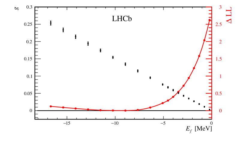
Figure 3: The coupling to the ${D}{\kern 1.79997pt\overline{\kern-1.79997ptD}{}}^{*}$ channels $g$ as a function of Flatté energy parameter $E_{f}$ (black points with error bars). The corresponding change in negative log likelihood, $\Delta\mathrm{LL}$ is shown as well (red dots).

Table 4: Results from the constrained Flatté fit. The uncertainties are statistical.

$g$	$f_{\rho}\times 10^{3}$	$\Gamma_{0}\,\left[\!\mathrm{\,Me\kern-1.00006ptV}\right]$	$m_{0}\,\left[\!\mathrm{\,Me\kern-1.00006ptV}\right]$
$0.108\pm 0.003$	$1.8\pm 0.6$	$1.4\pm 0.4$	$3864.5\,{\mathrm{(fixed)}}$

Table 5: Systematic uncertainty on the measurement of the Flatté parameters.

Systematic	$g$		$f_{\rho}\times 10^{3}$		$\Gamma_{0}~{}\left[\!\mathrm{\,Me\kern-1.00006ptV}\right]$
Model	$~{}~{}+0.003$	$-0.004~{}~{}$	$~{}~{}+0.6$	$-0.5~{}~{}$	$~{}~{}+0.5$	$-0.4~{}~{}$
Momentum scale	$~{}~{}+0.003$	$-0.003~{}~{}$	$~{}~{}+0.1$	$-0.2~{}~{}$	$~{}~{}+0.1$	$-0.2~{}~{}$
Threshold mass	$~{}~{}+0.003$	$-0.003~{}~{}$	$~{}~{}+0.2$	$-0.2~{}~{}$	$~{}~{}+0.2$	$-0.3~{}~{}$
${D}^{*0}$ width		$-0.001~{}~{}$				$-0.2~{}~{}$
Sum in quadrature	$~{}~{}+0.005$	$-0.006~{}~{}$	$~{}~{}+0.7$	$-0.6~{}~{}$	$~{}~{}+0.6$	$-0.6~{}~{}$

The systematic uncertainties on the Flatté parameters are summarised in Table 5 and discussed below. The systematic uncertainties introduced by the background and resolution parameterisations are evaluated in the same way as for the Breit–Wigner analysis, using discrete profiling. The impact of the momentum scale uncertainty is investigated by shifting the data points by $66\mathrm{\,ke\kern-1.00006ptV}$ and repeating the fit. Further systematic uncertainties are particular to the Flatté parameterisation. The location of the ${{D}^{0}}{{\kern 1.99997pt\overline{\kern-1.99997ptD}{}}{}^{*0}}$ threshold is known to a precision of $0.11\mathrm{\,Me\kern-1.00006ptV}$ [33]. Varying the threshold by this amount and repeating the fit leads to an uncertainty on the parameters which is similar to that introduced by the momentum scale. Finally, the ${{D}^{*0}}$ meson has a finite natural width, for which an upper limit of $\Gamma_{{{D}^{*0}}}<2.1\mathrm{\,Me\kern-1.00006ptV}$ [33] has been measured. However, theoretical predictions estimate $\Gamma_{D^{*}}=65.5\pm 15.4\,\mathrm{\,ke\kern-1.00006ptV}$ [40], based on the measured width of the ${{D}^{*+}}$ meson. Modified lineshape models taking into account the finite width of the ${{D}^{*0}}$ are available. In particular, Refs. [40, 47] suggest replacing $k_{1}(E)$ in Eq. (3) with

$$k^{\prime}_{1}(E)=\sqrt{-2\mu\left(E-E_{R}+i\Gamma_{{{D}^{*0}}}/2\right)}\,,$$ (9)

where $E_{R}\equiv m_{{{D}^{*0}}}-m_{{{D}^{0}}}-m_{{{\pi}^{0}}}$. The reduced mass, $\mu$, is calculated as $\tfrac{m_{{{D}^{0}}}(m_{{{D}^{0}}}+m_{{{\pi}^{0}}})}{(2m_{{{D}^{0}}}+m_{{{\pi}^{0}}})}$. With this modification there is always a contribution to both the imaginary and real part of the denominator function in Eq. (2). Repeating the fit results in a similar but worse fit quality with a log-likelihood difference of $0.1$. The width $\Gamma_{0}$ is reduced by $0.2\,\mathrm{\,Me\kern-1.00006ptV}$, which is the smallest systematic uncertainty on this parameter.

7.3 Comparison between Breit–Wigner and Flatté lineshapes

Figure 4 shows the comparison between the Breit–Wigner and the Flatté lineshapes. While in both cases the signal peaks at the same mass, the Flatté model results in a signifcantly narrower lineshape. However, after folding with the resolution function and adding the background, the observable distributions are indistinguishable.

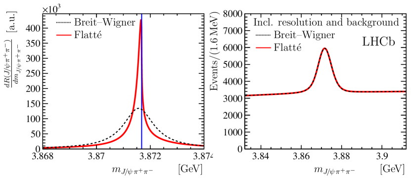
Figure 4: Comparison of the Flatté (solid, red) and Breit–Wigner (dotted, black) lineshapes. The left plot shows the raw lineshapes for the default fits. The location of the ${D}^{0}$ ${\kern 1.79997pt\overline{\kern-1.79997ptD}{}}{}^{*0}$ threshold is indicated by the blue vertical line. On the right the distributions are shown after applying smearing with the resolution function and adding background.

Table 6: Results of the fit with the Flatté lineshape including statistical and systematic uncertainties. The Flatté mass parameter $m_{0}=3864.5\mathrm{\,Me\kern-0.90005ptV}$ is used.

Mode $\left[\!\mathrm{\,Me\kern-1.00006ptV}\right]$	Mean $\left[\!\mathrm{\,Me\kern-1.00006ptV}\right]$	FWHM $\left[\!\mathrm{\,Me\kern-1.00006ptV}\right]$
$3871.69^{\,+\,0.00\,+\,0.05}_{\,-\,0.04\,-\,0.13}$	$3871.66^{\,+\,0.07\,+\,0.11}_{\,-\,0.06\,-\,0.13}$	$0.22^{\,+\,0.06\,+\,0.25}_{\,-\,0.08\,-\,0.17}$

To quantify this comparison the fit results for the mode, the mean and the full width at half-maximum (FWHM) of the Flatté model and their uncertainties are summarised in Table 6. The mode of the Flatté distribution agrees within uncertainties with the Breit–Wigner solution. However, the FWHM of the Flatté model is a factor of five smaller than the Breit–Wigner width. To check the consistency of these seemingly contradictory results, pseudoexperiments generated with the Flatté model and folded with the known resolution function are analysed with the Breit–Wigner model. Figure 5 shows the resulting distribution of the Breit–Wigner width determined from the pseudoexperiments, which is in good agreement with the value observed in the data. This demonstrates that the value obtained for the Breit–Wigner width, after taking into account the experimental resolution, is consistent with the expectation of the Flatté model. The result highlights the importance of a proper lineshape parameterisation for a measurement of the location of the pole.

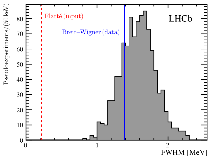
Figure 5: Distribution of the FWHM obtained for simulated experiments generated from the result of the Flatté model and fitted with the Breit–Wigner model (filled histogram). Both models account for the experimental resolution. The dashed red line shows the FWHM of the Flatté lineshape, while the solid blue line indicates the value of the Breit–Wigner width observed in data.

7.4 Pole search

The amplitude as a function of the energy defined by Eq. (2) can be continued analytically to complex values of the energy $E$. This continuation is valid up to singularities of the amplitude. There are two types of singularities, which are relevant here: poles and branch points. Poles of the amplitude in the complex energy plane are identified with hadronic states. The pole location is a unique property of the respective state, which is independent of the production process and the observed decay mode. In the absence of nearby thresholds the real part of the pole is located at the mass of the hadron and the imaginary part at half the width of the state. Branch point singularities occur at the threshold of every coupled channel and lead to branch cuts in the Riemann surface on which the amplitude is defined. Each branch cut corresponds to two Riemann sheets. Through Eq. (2) the amplitude will inherit the analytic structure of the square root functions of Eq. (3) that describe the momenta of the decay products in the rest frame of the two-body system. The square root is a two-sheeted function of complex energy. In the following, a convention is used where the two sheets are connected along the negative real axis. An introduction to this subject can be found in Refs. [48, 49, 50] and a summary is available in Ref. [51].

For the ${\chi_{{c}1}}(3872)$ state only the Riemann sheets associated to the ${{D}^{0}}{{\kern 1.99997pt\overline{\kern-1.99997ptD}{}}{}^{*0}}$ channel are important, since all other thresholds are far from the signal region. The following convention is adopted to label the relevant sheets:

1. $E-E_{f}-\dfrac{g}{2}\left(+\sqrt{-2\mu_{1}E}+\sqrt{-2\mu_{2}(E-\delta)}\right)+\dfrac{i}{2}\Gamma(E)$ with $\operatorname{Im}E>0$ ,

2. $E-E_{f}-\dfrac{g}{2}\left(+\sqrt{-2\mu_{1}E}+\sqrt{-2\mu_{2}(E-\delta)}\right)+\dfrac{i}{2}\Gamma(E)$ with $\operatorname{Im}E<0$ ,

3. $E-E_{f}-\dfrac{g}{2}\left(-\sqrt{-2\mu_{1}E}+\sqrt{-2\mu_{2}(E-\delta)}\right)+\dfrac{i}{2}\Gamma(E)$ with $\operatorname{Im}E<0$ ,

4. $E-E_{f}-\dfrac{g}{2}\left(-\sqrt{-2\mu_{1}E}+\sqrt{-2\mu_{2}(E-\delta)}\right)+\dfrac{i}{2}\Gamma(E)$ with $\operatorname{Im}E>0$ ,

where $\Gamma(E)\equiv\Gamma_{\rho}(E)+\Gamma_{\omega}(E)+\Gamma_{0}$. The fact that the model contains several coupled channels in addition to the ${{D}^{0}}{{\kern 1.99997pt\overline{\kern-1.99997ptD}{}}{}^{*0}}$ channel complicates the analytical structure. The sign in front of the momentum $\sqrt{-2\mu_{1}E}$ is the same for sheets I and II and therefore they belong to a single sheet with respect to the ${{D}^{0}}{{\kern 1.99997pt\overline{\kern-1.99997ptD}{}}{}^{*0}}$ channel. The two regions are labelled separately due to the presence of the the ${{J\mskip-3.0mu/\mskip-2.0mu\psi\mskip 2.0mu}}{{\pi}^{+}}{{\pi}^{-}}$, ${{J\mskip-3.0mu/\mskip-2.0mu\psi\mskip 2.0mu}}{{\pi}^{+}}{{\pi}^{-}}{{\pi}^{0}}$ channels, as well as radiative decays. Those channels have their associated branch points at smaller masses than the signal region. The analysis is performed close to the ${{D}^{0}}{{\kern 1.99997pt\overline{\kern-1.99997ptD}{}}{}^{*0}}$ threshold and points above and below the real axis lie on different sheets with respect to those open channels.

Sheets I and II correspond to a physical sheet with respect to the ${{D}^{0}}{{\kern 1.99997pt\overline{\kern-1.99997ptD}{}}{}^{*0}}$ channel, where the amplitude is evaluated in order to compute the measurable lineshape at real energies $E$. Sheets III and IV correspond to an unphysical sheet with respect to that channel. Sheet II is analytically connected to sheet IV along the real axis, above the ${{D}^{0}}{{\kern 1.99997pt\overline{\kern-1.99997ptD}{}}{}^{*0}}$ threshold.

In the single-channel case, a bound ${{D}^{0}}{{\kern 1.99997pt\overline{\kern-1.99997ptD}{}}{}^{*0}}$ state would appear below threshold on the real axis and on the physical sheet.

A virtual state would appear as well below threshold on the real axis, but on the unphysical sheet. A resonance would appear on the unphysical sheet in the complex plane [48, 49, 50]. The presence of inelastic, open channels shifts the pole into the complex plane and turns both a bound state as well as a virtual state into resonances. In the implementation of the amplitude used for the analysis, the branch cut for the ${{D}^{0}}{{\kern 1.99997pt\overline{\kern-1.99997ptD}{}}{}^{*0}}$ channel is taken to go from threshold towards larger energy $E$, while the branch cuts associated to the open channels $\Gamma(E)$ are chosen to lie along the negative real axis. The analytic structure around the branch cut associated to the ${{D}^{+}}{{D}^{*-}}$ threshold is also investigated, but no nearby poles are found on the respective Riemann sheets.

At the best estimate of the Flatté parameters the model exhibits two pole singularities. The first pole appears on sheet II and is located very close to the ${{D}^{0}}{{\kern 1.99997pt\overline{\kern-1.99997ptD}{}}{}^{*0}}$ threshold . The location of this pole with respect to the branch point, obtained using the algorithm described in Ref. [52], is $E_{\mathrm{II}}=(0.06-0.13\>i)\mathrm{\,Me\kern-1.00006ptV}$. Recalling that the imaginary part of the pole position corresponds to half the visible width, it is clear that this pole is responsible for the peaking region of the lineshape. A second pole is found on sheet III. It appears well below the threshold and is also further displaced from the physical axis at $E_{\mathrm{III}}=(-3.58-1.22\>i)\mathrm{\,Me\kern-1.00006ptV}$.

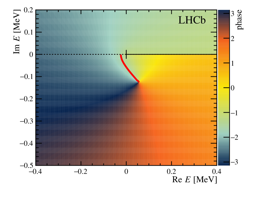
Figure 6: The phase of the Flatté amplitude obtained from the fit to the data with $m_{0}=3864.5\mathrm{\,Me\kern-0.90005ptV}$ on sheets I (for $\operatorname{Im}E>0$) and II (for $\operatorname{Im}E<0$) of the complex energy plane. The pole singularity is visible at $E_{\mathrm{II}}=(0.06-0.13\>i)\mathrm{\,Me\kern-0.90005ptV}$. The branch cut is highlighted with the black line. The trajectory of the pole taken when the couplings to all but the ${D}{{\kern 1.79997pt\overline{\kern-1.79997ptD}{}}{}^{*}}$ channel are scaled down to zero is indicated in red.

Figure 6 shows the analytic structure of the Flatté amplitude in the vicinity of the threshold. The color code corresponds to the phase of the amplitude on sheets I (for $\operatorname{Im}E>0$) and II (for $\operatorname{Im}E<0$) in the complex energy plane. The pole on sheet II is visible, as is the discontinuity along the ${{D}^{0}}{{\kern 1.99997pt\overline{\kern-1.99997ptD}{}}{}^{*0}}$ branch cut, which for clarity is also indicated by the black line. The trajectory followed by the pole when taking the limit where the couplings to all channels but ${{D}^{0}}{{\kern 1.99997pt\overline{\kern-1.99997ptD}{}}{}^{*0}}$ are sent to zero is shown in red and discussed below.

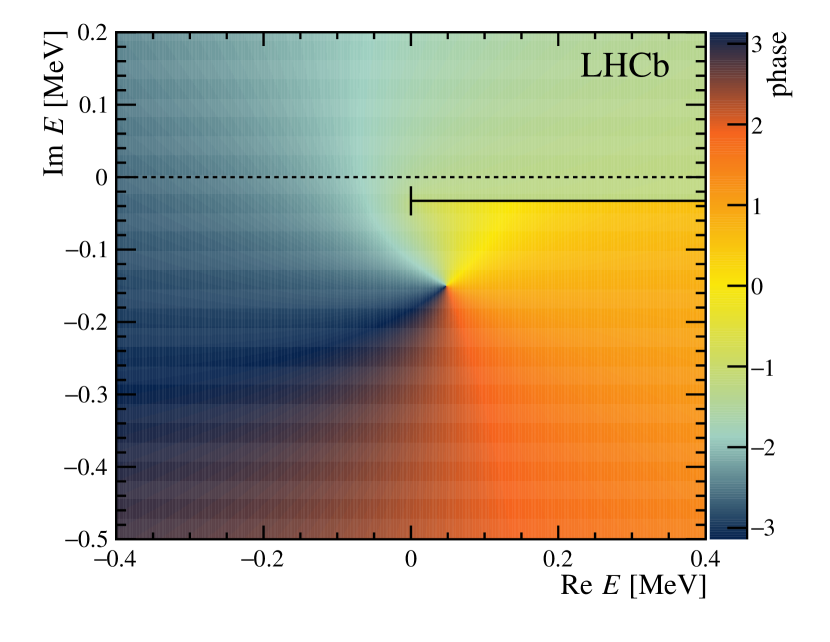
Figure 7: The phase of the Flatté amplitude as obtained from the fit with a finite ${D}^{*0}$ width of $\Gamma_{{D}^{*0}}=65.5\mathrm{\,ke\kern-0.90005ptV}$ on sheets I (for $\operatorname{Im}E>-\Gamma_{{{D}^{*0}}}/2$) and II (for $\operatorname{Im}E<-\Gamma_{{{D}^{*0}}}/2$) of the complex energy plane. Since the ${\kern 1.79997pt\overline{\kern-1.79997ptD}{}}{}^{*0}$ meson is treated as an unstable particle, the ${D}^{0}$ ${\kern 1.79997pt\overline{\kern-1.79997ptD}{}}{}^{*0}$ branch cut, indicated by the black solid line, is located at $\operatorname{Im}E=-\Gamma_{{{D}^{*0}}}/2$. The location of the pole is on the physical sheet with respect to the ${D}^{0}$ ${\kern 1.79997pt\overline{\kern-1.79997ptD}{}}{}^{*0}$ system.

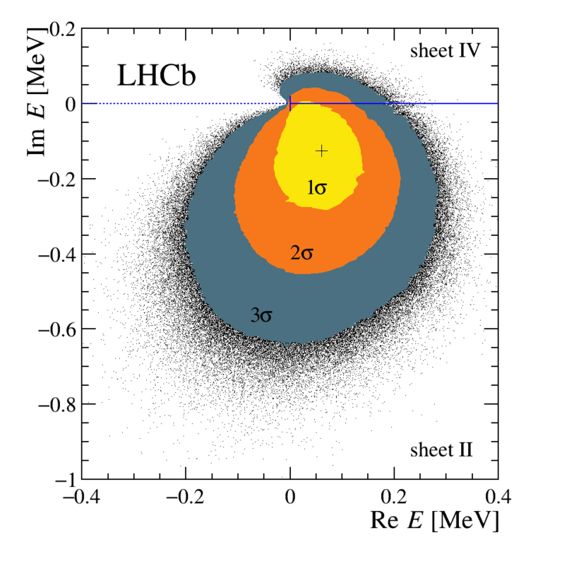
Figure 8: Confidence regions for the pole position on sheets II and IV in the complex energy plane. The displayed uncertainties include statistical contributions and the modeling uncertainty. The poles are extracted at a Flatté mass point of $m_{0}=3864.5\mathrm{\,Me\kern-0.90005ptV}$. The shaded areas are the 1, 2 and 3$\sigma$ confidence regions. The branch cut is shown as the blue line. The location of the branch cut singularity is indicated with a vertical bar at $E=0+0\>i$. The best estimates for the pole position is indicated by a cross. The black points indicate the samples from the pseudoexperiments procedure that lie outside the $3\sigma$ region.

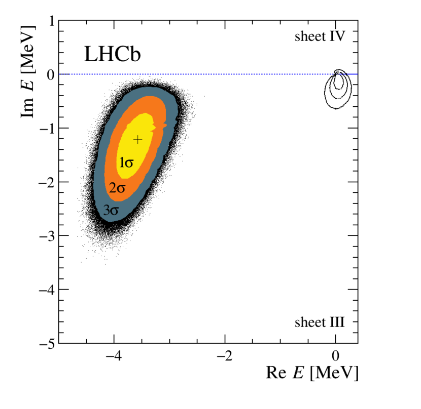
Figure 9: Confidence regions for the pole position on sheet III in the complex energy plane. The displayed uncertainties include statistical contributions and the modeling uncertainty. The poles are extracted at a Flatté mass point of $m_{0}=3864.5\mathrm{\,Me\kern-0.90005ptV}$. The shaded areas are the 1, 2 and 3$\sigma$ confidence regions. The branch cut is shown as the blue line. The location of the branch cut singularity is indicated with a vertical bar at $E=0+0\>i$. The best estimate for the pole positions is indicated by a cross. The confidence region for the pole on sheets II/IV is shown in outline for comparison. The black points indicate the samples from the pseudoexperiments procedure that lie outside the $3\sigma$ region.

As shown in Table 5, taking into account the finite width of the ${\kern 1.99997pt\overline{\kern-1.99997ptD}{}}{}^{*0}$ has a small effect on the Flatté parameters. However, the analytic structure of the amplitude close to the threshold is changed such that in this case the branch cut is located in the complex plane at $\operatorname{Im}E=-\Gamma_{{{D}^{*0}}}/2$. The phase of the amplitude for this case is shown in Fig. 7. The displaced branch cut is highlighted in black. The pole is found at $E^{\prime}_{\mathrm{II}}=(25-140\>i)\mathrm{\,ke\kern-1.00006ptV}$ in a similar location to the case without taking into account the ${\kern 1.99997pt\overline{\kern-1.99997ptD}{}}{}^{*0}$ width. In particular, the most likely pole position is on sheet II, the physical sheet with respect to the ${D}^{0}$ ${\kern 1.99997pt\overline{\kern-1.99997ptD}{}}{}^{*0}$ system. The location of the pole on sheet III is found to be $E^{\prime}_{\mathrm{III}}=(-3.59-1.05\>i)\mathrm{\,Me\kern-1.00006ptV}$, similar to the fit that does not account for ${\kern 1.99997pt\overline{\kern-1.99997ptD}{}}{}^{*0}$ width.

The uncertainties of the Flatté parameters are propagated to the pole position by generating large sets of pseudoexperiments, sampling from the asymmetric Gaussian uncertainties that describe the statistical and the systematic uncertainties introduced through the resolution and background parameterisation. The systematic uncertainty on the pole position due to the momentum scale, location of the threshold and the choice of the Flatté mass parameter are discussed in the following.

The confidence regions for the location of the poles, corresponding to $68.3\%,95.4\%$ and $99.7\%$ intervals, are shown in Figures  8 and 9. For large values of $g$ the pole on sheet II moves to sheet IV, which is analytically connected to the former along the real axis above threshold. Therefore, sheet II (for $\operatorname{Im}E<0$) and sheet IV (for $\operatorname{Im}E>0$) are shown together for this pole. While a pole location on sheet II is preferred by the data, a location on sheet IV is still allowed at the $2\sigma$ level. The pole on sheet III is located well below threshold and comparatively deep in the complex plane and is shown in Fig. 9. For comparison, the location of the confidence region for the first pole on sheets II and IV are also indicated on sheet III.

The positions of both poles depend on the choice of the Flatté mass parameter $m_{0}$. The dependence of the lineshape on $m_{0}$ has been explored in the region below threshold and for the results shown in Fig. 3 the corresponding pole positions are evaluated. The location of the pole on sheet II extracted for $-17<E_{f}<0\,\mathrm{\,Me\kern-1.00006ptV}$ are marked by black circles in Fig. 10. For smaller values of $m_{0}$ the pole moves closer to the real axis, for values of $m_{0}$ approaching the threshold, the pole moves further into the complex plane. For all fits performed the best estimate for the location of the pole is on sheet II.

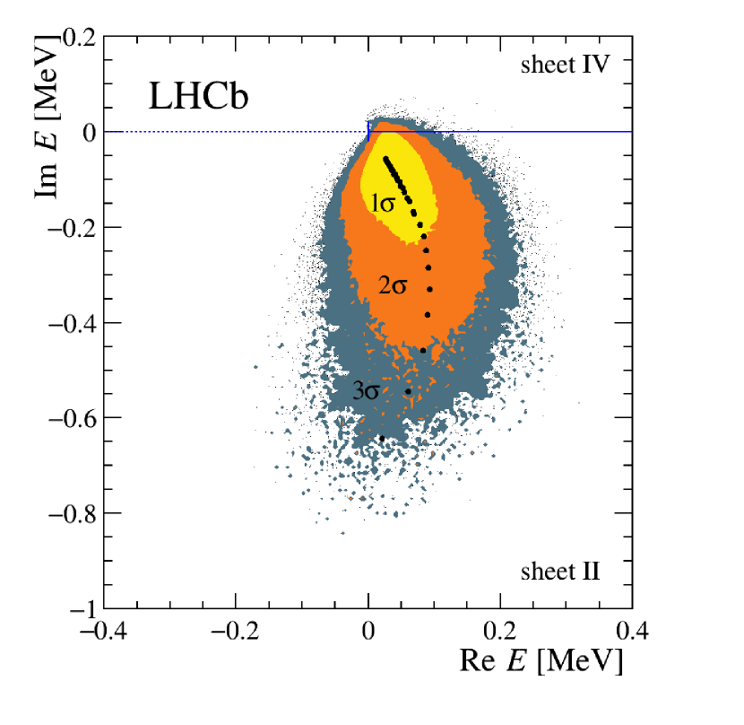
Figure 10: Confidence regions for the pole on sheet II in the complex energy plane. The displayed uncertainties include statistical contributions and the uncertainty from the choice of the Flatté mass parameter $m_{0}$. Modelling uncertainties are not shown. The shaded areas are the 1, 2 and 3$\sigma$ confidence regions. The branch cut is shown as the blue line. The location of the branch cut singularity is indicated with a vertical bar at $E=0+0\>i$. The black circles indicate the best estimates for the pole position for the different choices of $m_{0}$.

Figure 10 also shows the combined confidence regions, which account for the explored range of $E_{f}$. For each fit, a sample consisting of $10^{5}$ pseudoexperiments is drawn from the Gaussian distribution described by the covariance matrix of the fit parameters. Only the statistical uncertainties obtained for each fit are used for this study. The resulting samples of pole positions are combined by weighting with their respective likelihood ratios with respect to the best fit. The preferred location of the pole is on sheet II. However, a location of the pole on sheet IV is still allowed at the $2\sigma$ level.

The location of the pole on sheet III, in particular its real part, depends strongly on the choice of $m_{0}$. For small values of $m_{0}$ the pole moves away from the threshold and has less impact on the lineshape. For $m_{0}$ approaching the threshold this pole moves closer to the branch point and closer to the pole on sheet II. Since the asymmetry of the poles with respect to the threshold contains information on the potential molecular nature of the state [53], the values of the pole positions are provided for the most extreme scenario that is still allowed by the data with a likelihood difference of $\Delta\mathrm{LL}=1$, ($cf.$ Fig. 3) at $m_{0}=3869.3\mathrm{\,Me\kern-1.00006ptV}$. In this case the two poles are found at $E_{\mathrm{II}}=(0.09-0.33\>i)\mathrm{\,Me\kern-1.00006ptV}$ and $E_{\mathrm{III}}=(-0.85-0.97\>i)\mathrm{\,Me\kern-1.00006ptV}$.

The location of the threshold with respect to the observed location of the peak has a profound impact on the Flatté parameters and therefore on the pole position. The main uncertainties, which affect on which sheet the pole is found, are the knowledge of the momentum scale and the location of the ${{D}^{0}}{{\kern 1.99997pt\overline{\kern-1.99997ptD}{}}{}^{*0}}$ threshold. As shown in Table 5, both effects are of equal importance. Figure 11 shows the statistical uncertainties of the pole on sheet II for the case that the mass scale is shifted up by $66\mathrm{\,ke\kern-1.00006ptV}$. The pole is moving closer towards the real axis but the preferred location remains on sheet II. A measurement of the lineshape in the ${{D}^{0}}{{\kern 1.99997pt\overline{\kern-1.99997ptD}{}}{}^{*0}}$ channel is needed to further improve the knowledge on the impact of the threshold location.

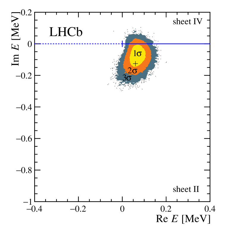
Figure 11: Confidence regions for the pole on sheet II in the complex energy plane, in the case that the mass scale is shifted up by $0.066\mathrm{\,Me\kern-0.90005ptV}$, due to systematic uncertainty of the momentum scale. Only the statistical uncertainties are displayed. The shaded areas are the 1, 2 and 3$\sigma$ confidence regions. The cross indicates the location of the pole found in the default fit, with the nominal momentum scale. The branch cut is shown as the blue line. The location of the branch cut singularity is indicated with a vertical bar at $E=0+0\>i$.

It is possible to study the behavior of the poles in the limit where only the ${D}{{\kern 1.99997pt\overline{\kern-1.99997ptD}{}}{}^{*}}$ channels are considered. The trajectory traced by the pole on sheet II when the couplings to the other channels ($f_{\rho}$, $f_{\omega}$, $\Gamma_{0}$) are sent to zero is indicated by the red curve in Fig. 6. The coupling $g$ and the Flatté mass parameter $E_{f}$ are kept fixed while taking this limit. For the best fit solution the pole moves below threshold and reaches the real axis at $E=-24\mathrm{\,ke\kern-1.00006ptV}$ staying on the physical sheet with respect to the ${{D}^{0}}{{\kern 1.99997pt\overline{\kern-1.99997ptD}{}}{}^{*0}}$ threshold. This location is consistent with a quasi-bound state in that channel with a binding energy of $E_{b}=24\,\mathrm{\,ke\kern-1.00006ptV}$. If the pole lies in the allowed region on sheet IV, taking the same limit also sends the pole onto the real axis below threshold, but on the unphysical sheet with respect to ${{D}^{0}}{{\kern 1.99997pt\overline{\kern-1.99997ptD}{}}{}^{*0}}$. This situation corresponds to a quasi-virtual state. Both types of solutions are analytically connected along the real axis through the branch cut singularity. Therefore, only upper limits on the binding energy can be set. For the bound state solution and only accounting for statistical uncertainties, the result is $E_{b}<57\mathrm{\,ke\kern-1.00006ptV}$ at 90% confidence level (CL). Including the systematic uncertainties due to the choice of the model this limit becomes $E_{b}<100\mathrm{\,ke\kern-1.00006ptV}$ at $90\%$ CL. Setting the couplings to the other channels to zero causes the pole on sheet III to move to the real axis as well, reaching it at $E=-3.51\mathrm{\,Me\kern-1.00006ptV}$. The corresponding values extracted at the highest allowed value of $m_{0}=3869.3\mathrm{\,Me\kern-1.00006ptV}$ are $E_{b}=29\mathrm{\,ke\kern-1.00006ptV}$ for the bound state pole and $E_{b}=0.73\mathrm{\,Me\kern-1.00006ptV}$ for the pole on the unphysical sheet.

8 Results and discussion

In this paper a large sample of ${\chi_{{c}1}}(3872)$ mesons from ${b}$-hadron decays collected by LHCb in 2011 and 2012 is exploited to study the lineshape of the ${\chi_{{c}1}}(3872)$ meson. Describing the lineshape with a Breit–Wigner function determines the mass splitting between the ${\chi_{{c}1}}(3872)$ and ${\psi{(2S)}}$ states to be

$$\Delta m=185.598\pm 0.067\pm 0.068\mathrm{\,Me\kern-1.00006ptV}\,,$$

where the first uncertainty is statistical and the second systematic. Using the known value of the $\psi{(2S)}$ mass [33] this corresponds to

$$m_{{\chi_{{c}1}}(3872)}=3871.695\pm 0.067\pm 0.068\pm 0.010\mathrm{\,Me\kern-1.00006ptV}\,,$$

where the third uncertainty is due to the knowledge of the $\psi{(2S)}$ mass. The result is in good agreement with the current world average [33]. The uncertainty is improved by a factor of two compared to the best previous measurement by the CDF collaboration [4]. The measured value can also be compared to the threshold value, $m_{{{D}^{0}}}+m_{{{D}^{*0}}}=3871.70\pm 0.11\mathrm{\,Me\kern-1.00006ptV}$. The ${\chi_{{c}1}}(3872)$ mass, evaluated from the mean of a fit assuming the Breit–Wigner lineshape, is coincident with the ${{D}^{0}}{{\kern 1.99997pt\overline{\kern-1.99997ptD}{}}{}^{*0}}$ threshold within uncertainties, with $\delta E=0.01\pm 0.14\mathrm{\,Me\kern-1.00006ptV}$. A non-zero Breit-Wigner width of the ${\chi_{{c}1}}(3872)$ state is obtained with a value of

$$\Gamma_{\mathrm{BW}}=1.39\pm 0.24\pm 0.10\mathrm{\,Me\kern-1.00006ptV}.$$

The values found here for $m_{{\chi_{{c}1}}(3872)}$ and $\Gamma_{\mathrm{BW}}$ are in good agreement with a complementary analysis using fully reconstructed ${{B}^{+}}\rightarrow{\chi_{{c}1}}(3872){{K}^{+}}$ decays presented in Ref. [54] and combined therein.

Since $\left|\delta E\right|<\Gamma_{\mathrm{BW}}$, the value of $\Gamma_{\mathrm{BW}}$ needs to be interpreted with caution as coupled channel effects distort the lineshape. To elucidate this, fits using the Flatté parameterization discussed in Refs. [15, 16] are performed. The parameters are found to be

$$g = 0.108\pm 0.003^{\,+\,0.005}_{\,-\,0.006}\,,$$

$$f_{\rho} = \left(1.8\pm 0.6^{\,+\,0.7}_{\,-\,0.6}\right)\times 10^{-3}\,,$$

$$\Gamma_{0} = 1.4\pm 0.4\pm 0.6\mathrm{\,Me\kern-1.00006ptV}\,,$$

with $m_{0}$ fixed at $3864.5\mathrm{\,Me\kern-1.00006ptV}$. The mode of the Flatté distribution agrees with the mean of the Breit–Wigner lineshape. However, the determined FWHM is much smaller, $0.22^{\,+\,0.06\,+\,0.25}_{\,-\,0.08\,-\,0.17}\,\mathrm{\,Me\kern-1.00006ptV}$, highlighting the importance of a physically well-motivated lineshape parameterization. The sensitivity of the data to the tails of the mass distribution limits the extent to which the Flatté parameters can be determined, as is expected in the case of a strong coupling of the state to the ${{D}^{0}}{{\kern 1.99997pt\overline{\kern-1.99997ptD}{}}{}^{*0}}$ channel [46]. Values of the parameter $E_{f}$ above $-2.0\mathrm{\,Me\kern-1.00006ptV}$ are excluded at 90% confidence level. The allowed region below threshold is $-270<E_{f}<-2.0\mathrm{\,Me\kern-1.00006ptV}$. In this region a linear dependence between the parameters is observed. The slope $\frac{dg}{dE_{f}}$ is related to the real part of the scattering length [15] and is measured to be

$$\dfrac{dg}{dE_{f}}=\left(-15.11\pm 0.16\right)\mathrm{\,Ge\kern-1.00006ptV}^{-1}\,.$$

In order to investigate the nature of the ${\chi_{{c}1}}(3872)$ state, the analytic structure of the amplitude in the vicinity of the ${{D}^{0}}{{\kern 1.99997pt\overline{\kern-1.99997ptD}{}}{}^{*0}}$ threshold is examined. Using the Flatté amplitude, two poles are found. Both poles appear on unphysical sheets with respect to the ${{J\mskip-3.0mu/\mskip-2.0mu\psi\mskip 2.0mu}}{{\pi}^{+}}{{\pi}^{-}}$ channel and formally can be classified as resonances. With respect to the ${{D}^{0}}{{\kern 1.99997pt\overline{\kern-1.99997ptD}{}}{}^{*0}}$ channel, one pole appears on the physical sheet, the other on the unphysical sheet. This configuration, corresponding to a quasi-bound ${{D}^{0}}{{\kern 1.99997pt\overline{\kern-1.99997ptD}{}}{}^{*0}}$ state, is preferred for all scenarios studied in this paper. However, within combined statistical and systematic uncertainties a location of the first pole on the unphysical sheet is still allowed at the $2\sigma$ level and a quasi-virtual state assignment for the ${\chi_{{c}1}}(3872)$ state cannot be excluded.

For the preferred quasi-bound state scenario the $90\%$ CL upper limit of the ${{D}^{0}}{{\kern 1.99997pt\overline{\kern-1.99997ptD}{}}{}^{*0}}$ binding energy $E_{b}$ is found to be $100\,\mathrm{\,ke\kern-1.00006ptV}$. The asymmetry of the locations of the two poles, which is found to be substantial, provides information on the composition of the ${\chi_{{c}1}}(3872)$ state. In the case of a dominantly molecular nature of a state a single pole close to threshold is expected, while in the case of a compact state there should be two nearby poles [55]. The argument is equivalent to the Weinberg composition criterion [56] in the sense that the asymmetry of the pole location in momentum space determines the relative fractions of molecular and compact components in the ${\chi_{{c}1}}(3872)$ wave function [57]

$$\dfrac{\left|k_{2}\right|-\left|k_{1}\right|}{\left|k_{1}\right|+\left|k_{2}\right|}=1-Z\,.$$

Here $Z$ is the probability to find a compact component in the wave function. The momentum $\left|k_{1}\right|=6.8\mathrm{\,Me\kern-1.00006ptV}$ is obtained by inserting the binding energy of the bound state pole into Eq. (3). The corresponding value for the second pole is $\left|k_{2}\right|=82\mathrm{\,Me\kern-1.00006ptV}$ and therefore one obtains $Z=15\%$. The asymmetry of the poles depends on the choice of $m_{0}$. The asymmetry is reduced as the $m_{0}$ parameter approaches the threshold. The largest value for $m_{0}$ that is still compatible with the data is $3869.3\mathrm{\,Me\kern-1.00006ptV}$. In this case one obtains $Z=33\%$ and therefore the probability to find a compact component in the ${\chi_{{c}1}}(3872)$ wave function is less than a third. It should be noted that this argument depends on the extrapolation to the single channel case. For resonances the wave function normalisation used in the Weinberg criterion is not valid and $Z$ has to be replaced by an integral over the spectral density [57]. Nevertheless, the value obtained in this work is in agreement with the results of the analysis of the spectral density using Belle data [44, 58], presented in Ref. [16].

The results for the amplitude parameters and in particular the locations of the poles, are systematically limited. In the future, a combined analysis of the ${\chi_{{c}1}}(3872)\!\rightarrow{{J\mskip-3.0mu/\mskip-2.0mu\psi\mskip 2.0mu}}{{\pi}^{+}}{{\pi}^{-}}$ and ${\chi_{{c}1}}(3872)\!\rightarrow{{D}^{0}}{{\kern 1.99997pt\overline{\kern-1.99997ptD}{}}{}^{*0}}$ channels will make possible improvements to the knowledge on the amplitude parameters.

LHCb collaboration

R. Aaij³¹, C. Abellán Beteta⁴⁹, T. Ackernley⁵⁹, B. Adeva⁴⁵, M. Adinolfi⁵³, H. Afsharnia⁹, C.A. Aidala⁸², S. Aiola²⁵, Z. Ajaltouni⁹, S. Akar⁶⁴, J. Albrecht¹⁴, F. Alessio⁴⁷, M. Alexander⁵⁸, A. Alfonso Albero⁴⁴, Z. Aliouche⁶¹, G. Alkhazov³⁷, P. Alvarez Cartelle⁴⁷, A.A. Alves Jr⁴⁵, S. Amato², Y. Amhis¹¹, L. An²¹, L. Anderlini²¹, G. Andreassi⁴⁸, A. Andreianov³⁷, M. Andreotti²⁰, F. Archilli¹⁶, A. Artamonov⁴³, M. Artuso⁶⁷, K. Arzymatov⁴¹, E. Aslanides¹⁰, M. Atzeni⁴⁹, B. Audurier¹¹, S. Bachmann¹⁶, M. Bachmayer⁴⁸, J.J. Back⁵⁵, S. Baker⁶⁰, P. Baladron Rodriguez⁴⁵, V. Balagura^11,b, W. Baldini²⁰, J. Baptista Leite¹, R.J. Barlow⁶¹, S. Barsuk¹¹, W. Barter⁶⁰, M. Bartolini^23,47,h, F. Baryshnikov⁷⁹, J.M. Basels¹³, G. Bassi²⁸, V. Batozskaya³⁵, B. Batsukh⁶⁷, A. Battig¹⁴, A. Bay⁴⁸, M. Becker¹⁴, F. Bedeschi²⁸, I. Bediaga¹, A. Beiter⁶⁷, V. Belavin⁴¹, S. Belin²⁶, V. Bellee⁴⁸, K. Belous⁴³, I. Belyaev³⁸, G. Bencivenni²², E. Ben-Haim¹², S. Benson³¹, A. Berezhnoy³⁹, R. Bernet⁴⁹, D. Berninghoff¹⁶, H.C. Bernstein⁶⁷, C. Bertella⁴⁷, E. Bertholet¹², A. Bertolin²⁷, C. Betancourt⁴⁹, F. Betti^19,e, M.O. Bettler⁵⁴, Ia. Bezshyiko⁴⁹, S. Bhasin⁵³, J. Bhom³³, L. Bian⁷², M.S. Bieker¹⁴, S. Bifani⁵², P. Billoir¹², F.C.R. Bishop⁵⁴, A. Bizzeti^21,t, M. Bjørn⁶², M.P. Blago⁴⁷, T. Blake⁵⁵, F. Blanc⁴⁸, S. Blusk⁶⁷, D. Bobulska⁵⁸, V. Bocci³⁰, J.A. Boelhauve¹⁴, O. Boente Garcia⁴⁵, T. Boettcher⁶³, A. Boldyrev⁸⁰, A. Bondar^42,w, N. Bondar^37,47, S. Borghi⁶¹, M. Borisyak⁴¹, M. Borsato¹⁶, J.T. Borsuk³³, S.A. Bouchiba⁴⁸, T.J.V. Bowcock⁵⁹, A. Boyer⁴⁷, C. Bozzi²⁰, M.J. Bradley⁶⁰, S. Braun⁶⁵, A. Brea Rodriguez⁴⁵, M. Brodski⁴⁷, J. Brodzicka³³, A. Brossa Gonzalo⁵⁵, D. Brundu²⁶, E. Buchanan⁵³, A. Büchler-Germann⁴⁹, A. Buonaura⁴⁹, C. Burr⁴⁷, A. Bursche²⁶, A. Butkevich⁴⁰, J.S. Butter³¹, J. Buytaert⁴⁷, W. Byczynski⁴⁷, S. Cadeddu²⁶, H. Cai⁷², R. Calabrese^20,g, L. Calero Diaz²², S. Cali²², R. Calladine⁵², M. Calvi^24,i, M. Calvo Gomez^44,l, P. Camargo Magalhaes⁵³, A. Camboni⁴⁴, P. Campana²², D.H. Campora Perez³¹, A.F. Campoverde Quezada⁵, S. Capelli^24,i, L. Capriotti^19,e, A. Carbone^19,e, G. Carboni²⁹, R. Cardinale^23,h, A. Cardini²⁶, I. Carli⁶, P. Carniti^24,i, K. Carvalho Akiba³¹, A. Casais Vidal⁴⁵, G. Casse⁵⁹, M. Cattaneo⁴⁷, G. Cavallero⁴⁷, S. Celani⁴⁸, R. Cenci²⁸, J. Cerasoli¹⁰, A.J. Chadwick⁵⁹, M.G. Chapman⁵³, M. Charles¹², Ph. Charpentier⁴⁷, G. Chatzikonstantinidis⁵², M. Chefdeville⁸, C. Chen³, S. Chen²⁶, A. Chernov³³, S.-G. Chitic⁴⁷, V. Chobanova⁴⁵, S. Cholak⁴⁸, M. Chrzaszcz³³, A. Chubykin³⁷, V. Chulikov³⁷, P. Ciambrone²², M.F. Cicala⁵⁵, X. Cid Vidal⁴⁵, G. Ciezarek⁴⁷, F. Cindolo¹⁹, P.E.L. Clarke⁵⁷, M. Clemencic⁴⁷, H.V. Cliff⁵⁴, J. Closier⁴⁷, J.L. Cobbledick⁶¹, V. Coco⁴⁷, J.A.B. Coelho¹¹, J. Cogan¹⁰, E. Cogneras⁹, L. Cojocariu³⁶, P. Collins⁴⁷, T. Colombo⁴⁷, A. Contu²⁶, N. Cooke⁵², G. Coombs⁵⁸, S. Coquereau⁴⁴, G. Corti⁴⁷, C.M. Costa Sobral⁵⁵, B. Couturier⁴⁷, D.C. Craik⁶³, J. Crkovská⁶⁶, M. Cruz Torres^1,y, R. Currie⁵⁷, C.L. Da Silva⁶⁶, E. Dall’Occo¹⁴, J. Dalseno⁴⁵, C. D’Ambrosio⁴⁷, A. Danilina³⁸, P. d’Argent⁴⁷, A. Davis⁶¹, O. De Aguiar Francisco⁴⁷, K. De Bruyn⁴⁷, S. De Capua⁶¹, M. De Cian⁴⁸, J.M. De Miranda¹, L. De Paula², M. De Serio^18,d, D. De Simone⁴⁹, P. De Simone²², J.A. de Vries⁷⁷, C.T. Dean⁶⁶, W. Dean⁸², D. Decamp⁸, L. Del Buono¹², B. Delaney⁵⁴, H.-P. Dembinski¹⁴, A. Dendek³⁴, V. Denysenko⁴⁹, D. Derkach⁸⁰, O. Deschamps⁹, F. Desse¹¹, F. Dettori^26,f, B. Dey⁷, A. Di Canto⁴⁷, P. Di Nezza²², S. Didenko⁷⁹, H. Dijkstra⁴⁷, V. Dobishuk⁵¹, A.M. Donohoe¹⁷, F. Dordei²⁶, M. Dorigo^28,x, A.C. dos Reis¹, L. Douglas⁵⁸, A. Dovbnya⁵⁰, A.G. Downes⁸, K. Dreimanis⁵⁹, M.W. Dudek³³, L. Dufour⁴⁷, P. Durante⁴⁷, J.M. Durham⁶⁶, D. Dutta⁶¹, M. Dziewiecki¹⁶, A. Dziurda³³, A. Dzyuba³⁷, S. Easo⁵⁶, U. Egede⁶⁹, V. Egorychev³⁸, S. Eidelman^42,w, S. Eisenhardt⁵⁷, S. Ek-In⁴⁸, L. Eklund⁵⁸, S. Ely⁶⁷, A. Ene³⁶, E. Epple⁶⁶, S. Escher¹³, J. Eschle⁴⁹, S. Esen³¹, T. Evans⁴⁷, A. Falabella¹⁹, J. Fan³, Y. Fan⁵, B. Fang⁷², N. Farley⁵², S. Farry⁵⁹, D. Fazzini¹¹, P. Fedin³⁸, M. Féo⁴⁷, P. Fernandez Declara⁴⁷, A. Fernandez Prieto⁴⁵, F. Ferrari^19,e, L. Ferreira Lopes⁴⁸, F. Ferreira Rodrigues², S. Ferreres Sole³¹, M. Ferrillo⁴⁹, M. Ferro-Luzzi⁴⁷, S. Filippov⁴⁰, R.A. Fini¹⁸, M. Fiorini^20,g, M. Firlej³⁴, K.M. Fischer⁶², C. Fitzpatrick⁶¹, T. Fiutowski³⁴, F. Fleuret^11,b, M. Fontana⁴⁷, F. Fontanelli^23,h, R. Forty⁴⁷, V. Franco Lima⁵⁹, M. Franco Sevilla⁶⁵, M. Frank⁴⁷, E. Franzoso²⁰, G. Frau¹⁶, C. Frei⁴⁷, D.A. Friday⁵⁸, J. Fu^25,p, Q. Fuehring¹⁴, W. Funk⁴⁷, E. Gabriel⁵⁷, T. Gaintseva⁴¹, A. Gallas Torreira⁴⁵, D. Galli^19,e, S. Gallorini²⁷, S. Gambetta⁵⁷, Y. Gan³, M. Gandelman², P. Gandini²⁵, Y. Gao⁴, M. Garau²⁶, L.M. Garcia Martin⁴⁶, P. Garcia Moreno⁴⁴, J. García Pardiñas⁴⁹, B. Garcia Plana⁴⁵, F.A. Garcia Rosales¹¹, L. Garrido⁴⁴, D. Gascon⁴⁴, C. Gaspar⁴⁷, R.E. Geertsema³¹, D. Gerick¹⁶, E. Gersabeck⁶¹, M. Gersabeck⁶¹, T. Gershon⁵⁵, D. Gerstel¹⁰, Ph. Ghez⁸, V. Gibson⁵⁴, A. Gioventù⁴⁵, P. Gironella Gironell⁴⁴, L. Giubega³⁶, C. Giugliano^20,g, K. Gizdov⁵⁷, V.V. Gligorov¹², C. Göbel⁷⁰, E. Golobardes^44,l, D. Golubkov³⁸, A. Golutvin^60,79, A. Gomes^1,a, M. Goncerz³³, P. Gorbounov³⁸, I.V. Gorelov³⁹, C. Gotti^24,i, E. Govorkova³¹, J.P. Grabowski¹⁶, R. Graciani Diaz⁴⁴, T. Grammatico¹², L.A. Granado Cardoso⁴⁷, E. Graugés⁴⁴, E. Graverini⁴⁸, G. Graziani²¹, A. Grecu³⁶, L.M. Greeven³¹, P. Griffith^20,g, L. Grillo⁶¹, L. Gruber⁴⁷, B.R. Gruberg Cazon⁶², C. Gu³, M. Guarise²⁰, P. A. Günther¹⁶, E. Gushchin⁴⁰, A. Guth¹³, Yu. Guz^43,47, T. Gys⁴⁷, T. Hadavizadeh⁶⁹, G. Haefeli⁴⁸, C. Haen⁴⁷, S.C. Haines⁵⁴, P.M. Hamilton⁶⁵, Q. Han⁷, X. Han¹⁶, T.H. Hancock⁶², S. Hansmann-Menzemer¹⁶, N. Harnew⁶², T. Harrison⁵⁹, R. Hart³¹, C. Hasse⁴⁷, M. Hatch⁴⁷, J. He⁵, M. Hecker⁶⁰, K. Heijhoff³¹, K. Heinicke¹⁴, A.M. Hennequin⁴⁷, K. Hennessy⁵⁹, L. Henry^25,46, J. Heuel¹³, A. Hicheur⁶⁸, D. Hill⁶², M. Hilton⁶¹, S.E. Hollitt¹⁴, P.H. Hopchev⁴⁸, J. Hu¹⁶, J. Hu⁷¹, W. Hu⁷, W. Huang⁵, W. Hulsbergen³¹, T. Humair⁶⁰, R.J. Hunter⁵⁵, M. Hushchyn⁸⁰, D. Hutchcroft⁵⁹, D. Hynds³¹, P. Ibis¹⁴, M. Idzik³⁴, D. Ilin³⁷, P. Ilten⁵², A. Inglessi³⁷, K. Ivshin³⁷, R. Jacobsson⁴⁷, S. Jakobsen⁴⁷, E. Jans³¹, B.K. Jashal⁴⁶, A. Jawahery⁶⁵, V. Jevtic¹⁴, F. Jiang³, M. John⁶², D. Johnson⁴⁷, C.R. Jones⁵⁴, T.P. Jones⁵⁵, B. Jost⁴⁷, N. Jurik⁶², S. Kandybei⁵⁰, Y. Kang³, M. Karacson⁴⁷, J.M. Kariuki⁵³, N. Kazeev⁸⁰, M. Kecke¹⁶, F. Keizer^54,47, M. Kelsey⁶⁷, M. Kenzie⁵⁵, T. Ketel³², B. Khanji⁴⁷, A. Kharisova⁸¹, K.E. Kim⁶⁷, T. Kirn¹³, V.S. Kirsebom⁴⁸, O. Kitouni⁶³, S. Klaver²², K. Klimaszewski³⁵, S. Koliiev⁵¹, A. Kondybayeva⁷⁹, A. Konoplyannikov³⁸, P. Kopciewicz³⁴, R. Kopecna¹⁶, P. Koppenburg³¹, M. Korolev³⁹, I. Kostiuk^31,51, O. Kot⁵¹, S. Kotriakhova³⁷, P. Kravchenko³⁷, L. Kravchuk⁴⁰, R.D. Krawczyk⁴⁷, M. Kreps⁵⁵, F. Kress⁶⁰, S. Kretzschmar¹³, P. Krokovny^42,w, W. Krupa³⁴, W. Krzemien³⁵, W. Kucewicz^33,k, M. Kucharczyk³³, V. Kudryavtsev^42,w, H.S. Kuindersma³¹, G.J. Kunde⁶⁶, T. Kvaratskheliya³⁸, D. Lacarrere⁴⁷, G. Lafferty⁶¹, A. Lai²⁶, A. Lampis²⁶, D. Lancierini⁴⁹, J.J. Lane⁶¹, R. Lane⁵³, G. Lanfranchi²², C. Langenbruch¹³, O. Lantwin^49,79, T. Latham⁵⁵, F. Lazzari^28,u, R. Le Gac¹⁰, S.H. Lee⁸², R. Lefèvre⁹, A. Leflat^39,47, O. Leroy¹⁰, T. Lesiak³³, B. Leverington¹⁶, H. Li⁷¹, L. Li⁶², P. Li¹⁶, X. Li⁶⁶, Y. Li⁶, Y. Li⁶, Z. Li⁶⁷, X. Liang⁶⁷, T. Lin⁶⁰, R. Lindner⁴⁷, V. Lisovskyi¹⁴, R. Litvinov²⁶, G. Liu⁷¹, H. Liu⁵, S. Liu⁶, X. Liu³, A. Loi²⁶, J. Lomba Castro⁴⁵, I. Longstaff⁵⁸, J.H. Lopes², G. Loustau⁴⁹, G.H. Lovell⁵⁴, Y. Lu⁶, D. Lucchesi^27,n, S. Luchuk⁴⁰, M. Lucio Martinez³¹, V. Lukashenko³¹, Y. Luo³, A. Lupato⁶¹, E. Luppi^20,g, O. Lupton⁵⁵, A. Lusiani^28,s, X. Lyu⁵, L. Ma⁶, S. Maccolini^19,e, F. Machefert¹¹, F. Maciuc³⁶, V. Macko⁴⁸, P. Mackowiak¹⁴, S. Maddrell-Mander⁵³, L.R. Madhan Mohan⁵³, O. Maev³⁷, A. Maevskiy⁸⁰, D. Maisuzenko³⁷, M.W. Majewski³⁴, S. Malde⁶², B. Malecki⁴⁷, A. Malinin⁷⁸, T. Maltsev^42,w, H. Malygina¹⁶, G. Manca^26,f, G. Mancinelli¹⁰, R. Manera Escalero⁴⁴, D. Manuzzi^19,e, D. Marangotto^25,p, J. Maratas^9,v, J.F. Marchand⁸, U. Marconi¹⁹, S. Mariani^21,21,47, C. Marin Benito¹¹, M. Marinangeli⁴⁸, P. Marino⁴⁸, J. Marks¹⁶, P.J. Marshall⁵⁹, G. Martellotti³⁰, L. Martinazzoli⁴⁷, M. Martinelli^24,i, D. Martinez Santos⁴⁵, F. Martinez Vidal⁴⁶, A. Massafferri¹, M. Materok¹³, R. Matev⁴⁷, A. Mathad⁴⁹, Z. Mathe⁴⁷, V. Matiunin³⁸, C. Matteuzzi²⁴, K.R. Mattioli⁸², A. Mauri⁴⁹, E. Maurice^11,b, M. Mazurek³⁵, M. McCann⁶⁰, L. Mcconnell¹⁷, T.H. Mcgrath⁶¹, A. McNab⁶¹, R. McNulty¹⁷, J.V. Mead⁵⁹, B. Meadows⁶⁴, C. Meaux¹⁰, G. Meier¹⁴, N. Meinert⁷⁵, D. Melnychuk³⁵, S. Meloni^24,i, M. Merk³¹, A. Merli²⁵, L. Meyer Garcia², M. Mikhasenko⁴⁷, D.A. Milanes⁷³, E. Millard⁵⁵, M.-N. Minard⁸, O. Mineev³⁸, L. Minzoni^20,g, S.E. Mitchell⁵⁷, B. Mitreska⁶¹, D.S. Mitzel⁴⁷, A. Mödden¹⁴, A. Mogini¹², R.A. Mohammed⁶², R.D. Moise⁶⁰, T. Mombächer¹⁴, I.A. Monroy⁷³, S. Monteil⁹, M. Morandin²⁷, G. Morello²², M.J. Morello^28,s, J. Moron³⁴, A.B. Morris¹⁰, A.G. Morris⁵⁵, R. Mountain⁶⁷, H. Mu³, F. Muheim⁵⁷, M. Mukherjee⁷, M. Mulder⁴⁷, D. Müller⁴⁷, K. Müller⁴⁹, C.H. Murphy⁶², D. Murray⁶¹, P. Muzzetto²⁶, P. Naik⁵³, T. Nakada⁴⁸, R. Nandakumar⁵⁶, T. Nanut⁴⁸, I. Nasteva², M. Needham⁵⁷, I. Neri^20,g, N. Neri^25,p, S. Neubert⁷⁴, N. Neufeld⁴⁷, R. Newcombe⁶⁰, T.D. Nguyen⁴⁸, C. Nguyen-Mau^48,m, E.M. Niel¹¹, S. Nieswand¹³, N. Nikitin³⁹, N.S. Nolte⁴⁷, C. Nunez⁸², A. Oblakowska-Mucha³⁴, V. Obraztsov⁴³, S. Ogilvy⁵⁸, D.P. O’Hanlon⁵³, R. Oldeman^26,f, C.J.G. Onderwater⁷⁶, J. D. Osborn⁸², A. Ossowska³³, J.M. Otalora Goicochea², T. Ovsiannikova³⁸, P. Owen⁴⁹, A. Oyanguren⁴⁶, B. Pagare⁵⁵, P.R. Pais⁴⁷, T. Pajero^28,47,28,s, A. Palano¹⁸, M. Palutan²², Y. Pan⁶¹, G. Panshin⁸¹, A. Papanestis⁵⁶, M. Pappagallo⁵⁷, L.L. Pappalardo^20,g, C. Pappenheimer⁶⁴, W. Parker⁶⁵, C. Parkes⁶¹, C.J. Parkinson⁴⁵, G. Passaleva^21,47, A. Pastore¹⁸, M. Patel⁶⁰, C. Patrignani^19,e, A. Pearce⁴⁷, A. Pellegrino³¹, M. Pepe Altarelli⁴⁷, S. Perazzini¹⁹, D. Pereima³⁸, P. Perret⁹, K. Petridis⁵³, A. Petrolini^23,h, A. Petrov⁷⁸, S. Petrucci⁵⁷, M. Petruzzo^25,p, A. Philippov⁴¹, L. Pica²⁸, B. Pietrzyk⁸, G. Pietrzyk⁴⁸, M. Pili⁶², D. Pinci³⁰, J. Pinzino⁴⁷, F. Pisani¹⁹, A. Piucci¹⁶, V. Placinta³⁶, S. Playfer⁵⁷, J. Plews⁵², M. Plo Casasus⁴⁵, F. Polci¹², M. Poli Lener²², M. Poliakova⁶⁷, A. Poluektov¹⁰, N. Polukhina^79,c, I. Polyakov⁶⁷, E. Polycarpo², G.J. Pomery⁵³, S. Ponce⁴⁷, A. Popov⁴³, D. Popov⁵², S. Popov⁴¹, S. Poslavskii⁴³, K. Prasanth³³, L. Promberger⁴⁷, C. Prouve⁴⁵, V. Pugatch⁵¹, A. Puig Navarro⁴⁹, H. Pullen⁶², G. Punzi^28,o, W. Qian⁵, J. Qin⁵, R. Quagliani¹², B. Quintana⁸, N.V. Raab¹⁷, R.I. Rabadan Trejo¹⁰, B. Rachwal³⁴, J.H. Rademacker⁵³, M. Rama²⁸, M. Ramos Pernas⁴⁵, M.S. Rangel², F. Ratnikov^41,80, G. Raven³², M. Reboud⁸, F. Redi⁴⁸, F. Reiss¹², C. Remon Alepuz⁴⁶, Z. Ren³, V. Renaudin⁶², R. Ribatti²⁸, S. Ricciardi⁵⁶, D.S. Richards⁵⁶, S. Richards⁵³, K. Rinnert⁵⁹, P. Robbe¹¹, A. Robert¹², G. Robertson⁵⁷, A.B. Rodrigues⁴⁸, E. Rodrigues⁵⁹, J.A. Rodriguez Lopez⁷³, M. Roehrken⁴⁷, A. Rollings⁶², V. Romanovskiy⁴³, M. Romero Lamas⁴⁵, A. Romero Vidal⁴⁵, J.D. Roth⁸², M. Rotondo²², M.S. Rudolph⁶⁷, T. Ruf⁴⁷, J. Ruiz Vidal⁴⁶, A. Ryzhikov⁸⁰, J. Ryzka³⁴, J.J. Saborido Silva⁴⁵, N. Sagidova³⁷, N. Sahoo⁵⁵, B. Saitta^26,f, C. Sanchez Gras³¹, C. Sanchez Mayordomo⁴⁶, R. Santacesaria³⁰, C. Santamarina Rios⁴⁵, M. Santimaria²², E. Santovetti^29,j, G. Sarpis⁶¹, M. Sarpis⁷⁴, A. Sarti³⁰, C. Satriano^30,r, A. Satta²⁹, M. Saur⁵, D. Savrina^38,39, H. Sazak⁹, L.G. Scantlebury Smead⁶², S. Schael¹³, M. Schellenberg¹⁴, M. Schiller⁵⁸, H. Schindler⁴⁷, M. Schmelling¹⁵, T. Schmelzer¹⁴, B. Schmidt⁴⁷, O. Schneider⁴⁸, A. Schopper⁴⁷, H.F. Schreiner⁶⁴, M. Schubiger³¹, S. Schulte⁴⁸, M.H. Schune¹¹, R. Schwemmer⁴⁷, B. Sciascia²², A. Sciubba²², S. Sellam⁶⁸, A. Semennikov³⁸, A. Sergi^52,47, N. Serra⁴⁹, J. Serrano¹⁰, L. Sestini²⁷, A. Seuthe¹⁴, P. Seyfert⁴⁷, D.M. Shangase⁸², M. Shapkin⁴³, L. Shchutska⁴⁸, T. Shears⁵⁹, L. Shekhtman^42,w, V. Shevchenko⁷⁸, E.B. Shields^24,i, E. Shmanin⁷⁹, J.D. Shupperd⁶⁷, B.G. Siddi²⁰, R. Silva Coutinho⁴⁹, L. Silva de Oliveira², G. Simi^27,n, S. Simone^18,d, I. Skiba^20,g, N. Skidmore⁷⁴, T. Skwarnicki⁶⁷, M.W. Slater⁵², J.C. Smallwood⁶², J.G. Smeaton⁵⁴, A. Smetkina³⁸, E. Smith¹³, I.T. Smith⁵⁷, M. Smith⁶⁰, A. Snoch³¹, M. Soares¹⁹, L. Soares Lavra⁹, M.D. Sokoloff⁶⁴, F.J.P. Soler⁵⁸, A. Solovev³⁷, I. Solovyev³⁷, F.L. Souza De Almeida², B. Souza De Paula², B. Spaan¹⁴, E. Spadaro Norella^25,p, P. Spradlin⁵⁸, F. Stagni⁴⁷, M. Stahl⁶⁴, S. Stahl⁴⁷, P. Stefko⁴⁸, O. Steinkamp^49,79, S. Stemmle¹⁶, O. Stenyakin⁴³, M. Stepanova³⁷, H. Stevens¹⁴, S. Stone⁶⁷, S. Stracka²⁸, M.E. Stramaglia⁴⁸, M. Straticiuc³⁶, D. Strekalina⁷⁹, S. Strokov⁸¹, F. Suljik⁶², J. Sun²⁶, L. Sun⁷², Y. Sun⁶⁵, P. Svihra⁶¹, P.N. Swallow⁵², K. Swientek³⁴, A. Szabelski³⁵, T. Szumlak³⁴, M. Szymanski⁴⁷, S. Taneja⁶¹, Z. Tang³, T. Tekampe¹⁴, F. Teubert⁴⁷, E. Thomas⁴⁷, K.A. Thomson⁵⁹, M.J. Tilley⁶⁰, V. Tisserand⁹, S. T’Jampens⁸, M. Tobin⁶, S. Tolk⁴⁷, L. Tomassetti^20,g, D. Torres Machado¹, D.Y. Tou¹², E. Tournefier⁸, M. Traill⁵⁸, M.T. Tran⁴⁸, E. Trifonova⁷⁹, C. Trippl⁴⁸, A. Tsaregorodtsev¹⁰, G. Tuci^28,o, A. Tully⁴⁸, N. Tuning³¹, A. Ukleja³⁵, D.J. Unverzagt¹⁶, A. Usachov³¹, A. Ustyuzhanin^41,80, U. Uwer¹⁶, A. Vagner⁸¹, V. Vagnoni¹⁹, A. Valassi⁴⁷, G. Valenti¹⁹, M. van Beuzekom³¹, H. Van Hecke⁶⁶, E. van Herwijnen⁷⁹, C.B. Van Hulse¹⁷, M. van Veghel⁷⁶, R. Vazquez Gomez⁴⁵, P. Vazquez Regueiro⁴⁵, C. Vázquez Sierra³¹, S. Vecchi²⁰, J.J. Velthuis⁵³, M. Veltri^21,q, A. Venkateswaran⁶⁷, M. Veronesi³¹, M. Vesterinen⁵⁵, J.V. Viana Barbosa⁴⁷, D. Vieira⁶⁴, M. Vieites Diaz⁴⁸, H. Viemann⁷⁵, X. Vilasis-Cardona⁴⁴, E. Vilella Figueras⁵⁹, P. Vincent¹², G. Vitali²⁸, A. Vitkovskiy³¹, A. Vollhardt⁴⁹, D. Vom Bruch¹², A. Vorobyev³⁷, V. Vorobyev^42,w, N. Voropaev³⁷, R. Waldi⁷⁵, J. Walsh²⁸, J. Wang³, J. Wang⁷², J. Wang⁴, J. Wang⁶, M. Wang³, R. Wang⁵³, Y. Wang⁷, Z. Wang⁴⁹, D.R. Ward⁵⁴, H.M. Wark⁵⁹, N.K. Watson⁵², S.G. Weber¹², D. Websdale⁶⁰, A. Weiden⁴⁹, C. Weisser⁶³, B.D.C. Westhenry⁵³, D.J. White⁶¹, M. Whitehead⁵³, D. Wiedner¹⁴, G. Wilkinson⁶², M. Wilkinson⁶⁷, I. Williams⁵⁴, M. Williams^63,69, M.R.J. Williams⁶¹, F.F. Wilson⁵⁶, W. Wislicki³⁵, M. Witek³³, L. Witola¹⁶, G. Wormser¹¹, S.A. Wotton⁵⁴, H. Wu⁶⁷, K. Wyllie⁴⁷, Z. Xiang⁵, D. Xiao⁷, Y. Xie⁷, H. Xing⁷¹, A. Xu⁴, J. Xu⁵, L. Xu³, M. Xu⁷, Q. Xu⁵, Z. Xu⁴, D. Yang³, Y. Yang⁵, Z. Yang³, Z. Yang⁶⁵, Y. Yao⁶⁷, L.E. Yeomans⁵⁹, H. Yin⁷, J. Yu⁷, X. Yuan⁶⁷, O. Yushchenko⁴³, K.A. Zarebski⁵², M. Zavertyaev^15,c, M. Zdybal³³, O. Zenaiev⁴⁷, M. Zeng³, D. Zhang⁷, L. Zhang³, S. Zhang⁴, Y. Zhang⁴⁷, A. Zhelezov¹⁶, Y. Zheng⁵, X. Zhou⁵, Y. Zhou⁵, X. Zhu³, V. Zhukov^13,39, J.B. Zonneveld⁵⁷, S. Zucchelli^19,e, D. Zuliani²⁷, G. Zunica⁶¹.

¹Centro Brasileiro de Pesquisas Físicas (CBPF), Rio de Janeiro, Brazil
²Universidade Federal do Rio de Janeiro (UFRJ), Rio de Janeiro, Brazil
³Center for High Energy Physics, Tsinghua University, Beijing, China
⁴School of Physics State Key Laboratory of Nuclear Physics and Technology, Peking University, Beijing, China
⁵University of Chinese Academy of Sciences, Beijing, China
⁶Institute Of High Energy Physics (IHEP), Beijing, China
⁷Institute of Particle Physics, Central China Normal University, Wuhan, Hubei, China
⁸Univ. Grenoble Alpes, Univ. Savoie Mont Blanc, CNRS, IN2P3-LAPP, Annecy, France
⁹Université Clermont Auvergne, CNRS/IN2P3, LPC, Clermont-Ferrand, France
¹⁰Aix Marseille Univ, CNRS/IN2P3, CPPM, Marseille, France
¹¹Université Paris-Saclay, CNRS/IN2P3, IJCLab, Orsay, France
¹²LPNHE, Sorbonne Université, Paris Diderot Sorbonne Paris Cité, CNRS/IN2P3, Paris, France
¹³I. Physikalisches Institut, RWTH Aachen University, Aachen, Germany
¹⁴Fakultät Physik, Technische Universität Dortmund, Dortmund, Germany
¹⁵Max-Planck-Institut für Kernphysik (MPIK), Heidelberg, Germany
¹⁶Physikalisches Institut, Ruprecht-Karls-Universität Heidelberg, Heidelberg, Germany
¹⁷School of Physics, University College Dublin, Dublin, Ireland
¹⁸INFN Sezione di Bari, Bari, Italy
¹⁹INFN Sezione di Bologna, Bologna, Italy
²⁰INFN Sezione di Ferrara, Ferrara, Italy
²¹INFN Sezione di Firenze, Firenze, Italy
²²INFN Laboratori Nazionali di Frascati, Frascati, Italy
²³INFN Sezione di Genova, Genova, Italy
²⁴INFN Sezione di Milano-Bicocca, Milano, Italy
²⁵INFN Sezione di Milano, Milano, Italy
²⁶INFN Sezione di Cagliari, Monserrato, Italy
²⁷INFN Sezione di Padova, Padova, Italy
²⁸INFN Sezione di Pisa, Pisa, Italy
²⁹INFN Sezione di Roma Tor Vergata, Roma, Italy
³⁰INFN Sezione di Roma La Sapienza, Roma, Italy
³¹Nikhef National Institute for Subatomic Physics, Amsterdam, Netherlands
³²Nikhef National Institute for Subatomic Physics and VU University Amsterdam, Amsterdam, Netherlands
³³Henryk Niewodniczanski Institute of Nuclear Physics Polish Academy of Sciences, Kraków, Poland
³⁴AGH - University of Science and Technology, Faculty of Physics and Applied Computer Science, Kraków, Poland
³⁵National Center for Nuclear Research (NCBJ), Warsaw, Poland
³⁶Horia Hulubei National Institute of Physics and Nuclear Engineering, Bucharest-Magurele, Romania
³⁷Petersburg Nuclear Physics Institute NRC Kurchatov Institute (PNPI NRC KI), Gatchina, Russia
³⁸Institute of Theoretical and Experimental Physics NRC Kurchatov Institute (ITEP NRC KI), Moscow, Russia, Moscow, Russia
³⁹Institute of Nuclear Physics, Moscow State University (SINP MSU), Moscow, Russia
⁴⁰Institute for Nuclear Research of the Russian Academy of Sciences (INR RAS), Moscow, Russia
⁴¹Yandex School of Data Analysis, Moscow, Russia
⁴²Budker Institute of Nuclear Physics (SB RAS), Novosibirsk, Russia
⁴³Institute for High Energy Physics NRC Kurchatov Institute (IHEP NRC KI), Protvino, Russia, Protvino, Russia
⁴⁴ICCUB, Universitat de Barcelona, Barcelona, Spain
⁴⁵Instituto Galego de Física de Altas Enerxías (IGFAE), Universidade de Santiago de Compostela, Santiago de Compostela, Spain
⁴⁶Instituto de Fisica Corpuscular, Centro Mixto Universidad de Valencia - CSIC, Valencia, Spain
⁴⁷European Organization for Nuclear Research (CERN), Geneva, Switzerland
⁴⁸Institute of Physics, Ecole Polytechnique Fédérale de Lausanne (EPFL), Lausanne, Switzerland
⁴⁹Physik-Institut, Universität Zürich, Zürich, Switzerland
⁵⁰NSC Kharkiv Institute of Physics and Technology (NSC KIPT), Kharkiv, Ukraine
⁵¹Institute for Nuclear Research of the National Academy of Sciences (KINR), Kyiv, Ukraine
⁵²University of Birmingham, Birmingham, United Kingdom
⁵³H.H. Wills Physics Laboratory, University of Bristol, Bristol, United Kingdom
⁵⁴Cavendish Laboratory, University of Cambridge, Cambridge, United Kingdom
⁵⁵Department of Physics, University of Warwick, Coventry, United Kingdom
⁵⁶STFC Rutherford Appleton Laboratory, Didcot, United Kingdom
⁵⁷School of Physics and Astronomy, University of Edinburgh, Edinburgh, United Kingdom
⁵⁸School of Physics and Astronomy, University of Glasgow, Glasgow, United Kingdom
⁵⁹Oliver Lodge Laboratory, University of Liverpool, Liverpool, United Kingdom
⁶⁰Imperial College London, London, United Kingdom
⁶¹Department of Physics and Astronomy, University of Manchester, Manchester, United Kingdom
⁶²Department of Physics, University of Oxford, Oxford, United Kingdom
⁶³Massachusetts Institute of Technology, Cambridge, MA, United States
⁶⁴University of Cincinnati, Cincinnati, OH, United States
⁶⁵University of Maryland, College Park, MD, United States
⁶⁶Los Alamos National Laboratory (LANL), Los Alamos, United States
⁶⁷Syracuse University, Syracuse, NY, United States
⁶⁸Laboratory of Mathematical and Subatomic Physics , Constantine, Algeria, associated to ^2
69School of Physics and Astronomy, Monash University, Melbourne, Australia, associated to ^55
70Pontifícia Universidade Católica do Rio de Janeiro (PUC-Rio), Rio de Janeiro, Brazil, associated to ^2
71Guangdong Provencial Key Laboratory of Nuclear Science, Institute of Quantum Matter, South China Normal University, Guangzhou, China, associated to ^3
72School of Physics and Technology, Wuhan University, Wuhan, China, associated to ^3
73Departamento de Fisica , Universidad Nacional de Colombia, Bogota, Colombia, associated to ^12
74Universität Bonn - Helmholtz-Institut für Strahlen und Kernphysik, Bonn, Germany, associated to ^16
75Institut für Physik, Universität Rostock, Rostock, Germany, associated to ^16
76Van Swinderen Institute, University of Groningen, Groningen, Netherlands, associated to ^31
77Universiteit Maastricht, Maastricht, Netherlands, associated to ^31
78National Research Centre Kurchatov Institute, Moscow, Russia, associated to ^38
79National University of Science and Technology “MISIS”, Moscow, Russia, associated to ^38
80National Research University Higher School of Economics, Moscow, Russia, associated to ^41
81National Research Tomsk Polytechnic University, Tomsk, Russia, associated to ^38
82University of Michigan, Ann Arbor, United States, associated to <sup>67

a</sup>Universidade Federal do Triângulo Mineiro (UFTM), Uberaba-MG, Brazil
^bLaboratoire Leprince-Ringuet, Palaiseau, France
^cP.N. Lebedev Physical Institute, Russian Academy of Science (LPI RAS), Moscow, Russia
^dUniversità di Bari, Bari, Italy
^eUniversità di Bologna, Bologna, Italy
^fUniversità di Cagliari, Cagliari, Italy
^gUniversità di Ferrara, Ferrara, Italy
^hUniversità di Genova, Genova, Italy
ⁱUniversità di Milano Bicocca, Milano, Italy
^jUniversità di Roma Tor Vergata, Roma, Italy
^kAGH - University of Science and Technology, Faculty of Computer Science, Electronics and Telecommunications, Kraków, Poland
^lDS4DS, La Salle, Universitat Ramon Llull, Barcelona, Spain
^mHanoi University of Science, Hanoi, Vietnam
ⁿUniversità di Padova, Padova, Italy
^oUniversità di Pisa, Pisa, Italy
^pUniversità degli Studi di Milano, Milano, Italy
^qUniversità di Urbino, Urbino, Italy
^rUniversità della Basilicata, Potenza, Italy
^sScuola Normale Superiore, Pisa, Italy
^tUniversità di Modena e Reggio Emilia, Modena, Italy
^uUniversità di Siena, Siena, Italy
^vMSU - Iligan Institute of Technology (MSU-IIT), Iligan, Philippines
^wNovosibirsk State University, Novosibirsk, Russia
^xINFN Sezione di Trieste, Trieste, Italy
^yUniversidad Nacional Autonoma de Honduras, Tegucigalpa, Honduras

References

- [1] E. S. Swanson, The new heavy mesons: a status report, Phys. Rept. 429 (2006) 243, arXiv:hep-ph/0601110
- [2] Belle collaboration, S. K. Choi et al., Observation of a narrow charmonium - like state in exclusive decays, Phys. Rev. Lett. 91 (2003) 262001, arXiv:hep-ex/0309032
- [3] BESIII collaboration, M. Ablikim et al., Observation of at BESIII, Phys. Rev. Lett. 112 (2014), no. 9 092001, arXiv:1310.4101
- [4] CDF collaboration, T. Aaltonen et al., Precision measurement of the mass in decays, Phys. Rev. Lett. 103 (2009) 152001, arXiv:0906.5218
- [5] BaBar collaboration, B. Aubert et al., A study of , with , Phys. Rev. D77 (2008) 111101, arXiv:0803.2838
- [6] D0 collaboration, V. M. Abazov et al., Observation and properties of the decaying to in collisions at TeV, Phys. Rev. Lett. 93 (2004) 162002, arXiv:hep-ex/0405004
- [7] LHCb collaboration, R. Aaij et al., Observation of production in collisions at , Eur. Phys. J. C72 (2012) 1972, arXiv:1112.5310
- [8] LHCb collaboration, R. Aaij et al., Determination of the meson quantum numbers, Phys. Rev. Lett. 110 (2013) 222001, arXiv:1302.6269
- [9] LHCb collaboration, R. Aaij et al., Quantum numbers of the state and orbital angular momentum in its decays, Phys. Rev. D92 (2015) 011102(R), arXiv:1504.06339
- [10] L. Maiani, F. Piccinini, A. D. Polosa, and V. Riquer, Diquark-antidiquarks with hidden or open charm and the nature of , Phys. Rev. D71 (2005) 014028, arXiv:hep-ph/0412098
- [11] N. A. Tornqvist, Isospin breaking of the narrow charmonium state of Belle at 3872 as a deuson, Phys. Lett. B590 (2004) 209, arXiv:hep-ph/0402237
- [12] C. Hanhart, Y. S. Kalashnikova, and A. V. Nefediev, Interplay of quark and meson degrees of freedom in a near-threshold resonance: multi-channel case, Eur. Phys. J. A47 (2011) 101, arXiv:1106.1185
- [13] BaBar collaboration, B. Aubert et al., Study of states produced in and , Phys. Rev. D73 (2006) 011101, arXiv:hep-ex/0507090
- [14] Belle collaboration, S.-K. Choi et al., Bounds on the width, mass difference and other properties of decays, Phys. Rev. D84 (2011) 052004, arXiv:1107.0163
- [15] C. Hanhart, Y. S. Kalashnikova, A. E. Kudryavtsev, and A. V. Nefediev, Reconciling the with the near-threshold enhancement in the final state, Phys. Rev. D76 (2007) 034007
- [16] Yu. S. Kalashnikova and A. V. Nefediev, Nature of from data, Phys. Rev. D80 (2009) 074004, arXiv:0907.4901
- [17] LHCb collaboration, A. A. Alves Jr. et al., The LHCb detector at the LHC, JINST 3 (2008) S08005
- [18] LHCb collaboration, R. Aaij et al., LHCb detector performance, Int. J. Mod. Phys. A30 (2015) 1530022, arXiv:1412.6352
- [19] R. Aaij et al., Performance of the LHCb Vertex Locator, JINST 9 (2014) P09007, arXiv:1405.7808
- [20] R. Arink et al., Performance of the LHCb Outer Tracker, JINST 9 (2014) P01002, arXiv:1311.3893
- [21] LHCb collaboration, R. Aaij et al., Measurements of the , , and baryon masses, Phys. Rev. Lett. 110 (2013) 182001, arXiv:1302.1072
- [22] LHCb collaboration, R. Aaij et al., Precision measurement of meson mass differences, JHEP 06 (2013) 065, arXiv:1304.6865
- [23] A. A. Alves Jr. et al., Performance of the LHCb muon system, JINST 8 (2013) P02022, arXiv:1211.1346
- [24] R. Aaij et al., The LHCb trigger and its performance in 2011, JINST 8 (2013) P04022, arXiv:1211.3055
- [25] T. Sjöstrand, S. Mrenna, and P. Skands, PYTHIA 6.4 physics and manual, JHEP 05 (2006) 026, arXiv:hep-ph/0603175
- [26] T. Sjöstrand, S. Mrenna, and P. Skands, A brief introduction to PYTHIA 8.1, Comput. Phys. Commun. 178 (2008) 852, arXiv:0710.3820
- [27] I. Belyaev et al., Handling of the generation of primary events in Gauss, the LHCb simulation framework, J. Phys. Conf. Ser. 331 (2011) 032047
- [28] D. J. Lange, The EvtGen particle decay simulation package, Nucl. Instrum. Meth. A462 (2001) 152
- [29] P. Golonka and Z. Was, PHOTOS Monte Carlo: A precision tool for QED corrections in and decays, Eur. Phys. J. C45 (2006) 97, arXiv:hep-ph/0506026
- [30] Geant4 collaboration, J. Allison et al., Geant4 developments and applications, IEEE Trans. Nucl. Sci. 53 (2006) 270
- [31] Geant4 collaboration, S. Agostinelli et al., Geant4: A simulation toolkit, Nucl. Instrum. Meth. A506 (2003) 250
- [32] M. Clemencic et al., The LHCb simulation application, Gauss: Design, evolution and experience, J. Phys. Conf. Ser. 331 (2011) 032023
- [33] Particle Data Group, M. Tanabashi et al., Review of particle physics, Phys. Rev. D98 (2018) 030001, and 2019 update
- [34] W. D. Hulsbergen, Decay chain fitting with a Kalman filter, Nucl. Instrum. Meth. A552 (2005) 566, arXiv:physics/0503191
- [35] W. S. McCulloch and W. Pitts, A logical calculus of the ideas immanent in nervous activity, The bulletin of mathematical biophysics 5 (1943), no. 4 115
- [36] F. Rosenblatt, The perceptron: A probabilistic model for information storage and organization in the brain, Psychological Review 65 (1958) 386
- [37] J.-H. Zhong et al., A program for the Bayesian neural network in the Root framework, Comput. Phys. Commun. 182 (2011) 2655, arXiv:1103.2854
- [38] H. Voss, A. Hoecker, J. Stelzer, and F. Tegenfeldt, TMVA - Toolkit for Multivariate Data Analysis, PoS ACAT (2007) 040
- [39] A. Hoecker et al., TMVA 4 — Toolkit for Multivariate Data Analysis. Users Guide., arXiv:physics/0703039
- [40] E. Braaten and M. Lu, Line shapes of the , Phys. Rev. D76 (2007) 094028, arXiv:0709.2697
- [41] E. Braaten and J. Stapleton, Analysis of and decays of the , Phys. Rev. D81 (2010) 014019, arXiv:0907.3167
- [42] T. Skwarnicki, A study of the radiative cascade transitions between the Upsilon-prime and Upsilon resonances, PhD thesis, Institute of Nuclear Physics, Krakow, 1986, DESY-F31-86-02
- [43] P. D. Dauncey et al., Handling uncertainties in background shapes: the discrete profiling method, JINST 10 (2015) P04015, arXiv:1408.6865
- [44] Belle collaboration, T. Aushev et al., Study of the decay, Phys. Rev. D81 (2010) 031103, arXiv:0810.0358
- [45] H.-X. Chen, W. Chen, X. Liu, and S.-L. Zhu, The hidden-charm pentaquark and tetraquark states, Phys. Rept. 639 (2016) 1, arXiv:1601.02092
- [46] V. Baru et al., Flattè-like distributions and the mesons, Eur. Phys. J. A 23 (2005) 523, arXiv:nucl-th/0410099
- [47] C. Hanhart, Y. S. Kalashnikova, and A. V. Nefediev, Lineshapes for composite particles with unstable constituents, Phys. Rev. D81 (2010) 094028, arXiv:1002.4097
- [48] R. J. Eden, P. V. Landshoff, D. I. Olive, and J. C. Polkinghorne, The analytic S-matrix, Cambridge Univ. Press, Cambridge, 1966
- [49] A. D. Martin and T. D. Spearman, Elementary Particle Theory, North-Holland Publishing Company, 1 ed., 1970
- [50] P. D. B. Collins, An Introduction to Regge Theory & High Energy Physics, Cambridge University Press, 1 ed., 1977
- [51] Resonances in Particle Data Group, M. Tanabashi et al., Review of particle physics, Phys. Rev. D98 (2018) 030001, 2019 update
- [52] P. Kowalczyk, Global complex roots and poles finding algorithm based on phase analysis for propagation and radiation problems, IEEE Transactions on Antennas and Propagation 66 (2018) 7198, arXiv:1806.06522
- [53] C. Hanhart, J. R. Pelaez, and G. Rios, Remarks on pole trajectories for resonances, Phys. Lett. B739 (2014) 375, arXiv:1407.7452
- [54] LHCb collaboration, R. Aaij et al., Study of the and states in the decays , arXiv:2005.13422, submitted to JHEP
- [55] D. Morgan, Pole counting and resonance classification, Nucl. Phys. A543 (1992) 632
- [56] S. Weinberg, Elementary particle theory of composite particles, Phys. Rev. 130 (1963) 776
- [57] V. Baru et al., Evidence that the and are not elementary particles, Phys. Lett. B586 (2004) 53
- [58] Belle collaboration, I. Adachi et al., Study of in meson decays, in 34th International Conference on High Energy Physics, 9, 2008. arXiv:0809.1224