Role of diffusive surface scattering in nonlocal plasmonics

Abstract

The recent generalised nonlocal optical response (GNOR) theory for plasmonics is analysed, and its main input parameter, namely the complex hydrodynamic convection-diffusion constant, is quantified in terms of enhanced Landau damping due to diffusive surface scattering of electrons at the surface of the metal. GNOR has been successful in describing plasmon damping effects, in addition to the frequency shifts originating from induced-charge screening, through a phenomenological electron diffusion term implemented into the traditional hydrodynamic Drude model of nonlocal plasmonics. Nevertheless, its microscopic derivation and justification is still missing. Here we discuss how the inclusion of a diffusion-like term in standard hydrodynamics can serve as an efficient vehicle to describe Landau damping without resorting to computationally demanding quantum-mechanical calculations, and establish a direct link between this term and the Feibelman $d$ parameter for the centroid of charge. Our approach provides a recipe to connect the phenomenological fundamental GNOR parameter to a frequency-dependent microscopic surface-response function. We therefore tackle one of the principal limitations of the model, and further elucidate its range of validity and limitations, thus facilitating its proper application in the framework of nonclassical plasmonics.

I Introduction

Increasing interest in spatial dispersion and the nonlocal response of plasmonic nanostructures is being observed in recent years, mainly due to its relevance for quantum plasmonics Tame:2013 ; Bozhevolnyi:2016a ; Bozhevolnyi:2016b ; Zhu:2016 ; Fitzgerald:2016 ; Yannopapas:2016 ; Amendola:2017 ; Fernandez-Dominguez:2018 ; Ciraci:2019 in a large number of experimentally available plasmonic architectures with ultrafine geometrical details Savage:2012 ; Duan:2012 ; Scholl:2012 ; Scholl:2013 ; Wiener:2013 ; Jung:2015 ; Raza:2015c ; Krasavin:2016 ; Shen:2017 . Hydrodynamic descriptions of the induced charges have been particularly emphasised Abajo:2008 ; McMahon:2010b ; Raza:2011 ; Ciraci:2012 ; David:2014 ; Christensen:2014 ; Raza:2015a ; Eremin:2018 ; Kupresak:2020 , and widely applied in situations where small particles or few-nm particle separations are involved. Relevant fully-quantum mechanical studies have shown that such models can in some occasions lead to qualitatively wrong conclusions, as, in their traditional implementation, they neglect electron spill-out Esteban:2012 ; Stella:2013 ; Teperik:2013a ; Yan:2015a ; Hohenester:2016 , an issue which is resolved once the hydrodynamic description is itself self-consistent Toscano:2015 ; Yan:2015b ; Ciraci:2016 . Nevertheless, despite these limitations, the hydrodynamic Drude model (HDM) still captures both qualitatively and to a large extent also quantitatively Raza:2013a the effect of nonlocal screening (due to spill-in promoted by a large work function) in noble metal nanostructures, and thus provides important insight into a wide range of experiments where spill-out and tunnelling can be safely disregarded, within a relatively simple and computationally efficient description. What it cannot capture, however, is the experimentally observed Kreibig:1970 , but theoretically challenging to quantify Kraus:1983 , broadening of the plasmonic modes with decreasing nanoparticle (NP) size. It is therefore useful to explore generalisations of HDM that enrich the physical description it provides.

One of the most successful extensions to the hydrodynamic description was achieved by the generalised nonlocal optical response (GNOR) theory Mortensen:2014 , which is based on a phenomenological inclusion of diffusion of free electrons in the bulk of the metal, to account for a series of experimentally observed plasmon damping mechanisms, including reduction of the electron mean-free path, quantum confinement and particularly Landau damping Apell:1984 ; Ouyang:1992 ; Baida:2009 ; Lerme:2010 ; Monreal:2013 ; Li:2013 ; Khurgin:2015a . These effects are reproduced within the GNOR theory by adding a classical diffusion term, introduced through a drift-diffusion equation, in the hydrodynamic description of free electrons, thus relaxing the necessity to resort to more computationally demanding quantum-mechanical descriptions Uskov:2014 ; Kirakosyan:2016 ; Shahbazyan:2016 ; Lerme:2017 . This formalism relies on a transport equation, established long ago for classical systems with stochastic scattering Chandrasekhar:1943 , i.e., convection-diffusion theory. The importance of both convection and diffusion for nonlocal electrodynamics was in fact predicted many years ago (see discussion in Landau-Lifshitz-Pitaevskii ). Diffusion has also been used as an abstract mathematical model to explain spatial dispersion Hanson:2010 , without however providing the physical link between diffusion dynamics and nonlocal plasmonic broadening. An early hint of how they can be connected through the fluctuation-dissipation theorem was given in Iwamoto:1984 . Despite these early estimations of the importance of diffusion, however, a more microscopic justification for its inclusion in nonlocal plasmonics in general, and in the GNOR theory in particular, is still missing, and the ambiguity in the choice of an appropriate hydrodynamic parameter restrains further extension of the applicability of such models.

Here we provide a microscopic foundation for the GNOR theory, following a procedure of gradually increasing complexity and getting deeper into the fine details of electron motion in a confined volume. Using the Boltzmann equation as our starting point, we first derive a diffusion correction to the continuity equation by assuming a weakly inhomogeneous initial electron density. We show that convection and diffusion are both manifestations of the same physical behaviour in the bulk, becoming important at different frequency limits, and diffusion is practically negligible at optical frequencies. To then justify the appearance of a diffusive term in the GNOR model, we turn to surface-scattering and Landau damping, and show how the GNOR diffusion constant relates to these effects. We derive a connection between the complex convection-diffusion hydrodynamic parameter and the Feibelman d parameters for the centroid of induced charge Feibelman:1982 , which quantifies the former through microscopic arguments. This approach is shown to provide a good agreement with the phenomenological size-dependent broadening (SDB) correction developed by Kreibig et al. Kreibig:1970 ; Kreibig:1985 in the case of a small metallic nanosphere, and it leads to reasonable broadening for other particle shapes, for which a simple SDB recipe is not available. Our procedure, which directly implements information retrieved from quantum-mechanical calculations, justifies and quantifies the phenomenological GNOR model, thus opening the pathway to its more widespread implementation in nonlocal/nonclassical plasmonics.

II Theoretical background

Throughout the paper we focus on the intraband response of free carriers, disregarding interband transitions. To begin with, Maxwell’s equations can be combined to obtain the wave equation

$${\boldsymbol{\nabla}}\times{\boldsymbol{\nabla}}\times\mathbf{E}=\left(\frac{\omega}{c}\right)^{2}\mathbf{E}+\mathrm{i}\omega\mu_{0}\mathbf{J}(\mathbf{E})~{},$$ (1)

where $\omega$ is the angular frequency of light, and $c=1/\sqrt{\varepsilon_{0}\mu_{0}}$ is the speed of light in vacuum, with $\varepsilon_{0}$ and $\mu_{0}$ representing the vacuum permittivity and permeability, respectively. The electrodynamic response of matter is contained in the constitutive relation between the current density $\mathbf{J}$ and the applied electric field $\mathbf{E}$, $\mathbf{J}(\mathbf{E})$. Within linear-response theory, the common local-response approximation (LRA) gives simply $\mathbf{J}(\mathbf{r})\simeq\sigma(\mathbf{r})\mathbf{E}(\mathbf{r})$ (Ohm’s law), where $\sigma(\mathbf{r})$ is the material conductivity, while in a nonlocal description we have Raza:2015a

$$\mathbf{J}(\mathbf{r})=\int\mathrm{d}\mathbf{r}^{\prime}\sigma(\mathbf{r},\mathbf{r}^{\prime})\mathbf{E}(\mathbf{r}^{\prime})~{}.$$ (2)

This expression states the fact that the induced current density at a point $\mathbf{r}$ inside the material should depend on the applied electric field at all neighbouring points $\mathbf{r}^{\prime}$. To proceed we need a theoretical model for $\mathbf{J}(\mathbf{E})$, and we will consider a hierarchy of increasing complexity, starting with the hydrodynamic drift-diffusion theory. The hydrodynamic approach is then justified through the Boltzmann transport equation, while additional insight from a microscopic account of surface scattering is provided for the diffusion term.

The hydrodynamic description relies on a classical equation of motion for an electron in an electromagnetic field, while accounting for quantum-pressure effects and multiple electron scattering in a semi-classical way. In the Boltzmann approach, quantum effects of the electron gas enter through scattering-matrix elements, where the non-convective, random velocity components are linked to classical diffusion. Finally, in the surface-scattering microscopic approach, first-principles surface-response functions, namely the Feibelman d parameters, are introduced to obtain a connection between the semi-classical convection and diffusion constants and the centroid of the induced charge.

III Hydrodynamic approach

Let us first briefly describe the procedure followed in the original introduction of GNOR theory Mortensen:2014 . We start with the linearised hydrodynamic equation of motion for an electron in an electric field Raza:2011 ; Boardman:1982a ; Tokatly:1999

$$\frac{\partial}{\partial t}\boldsymbol{\nu}=-\gamma\boldsymbol{\nu}+\frac{(-e)}{m}\mathbf{E}-\frac{\beta^{2}}{n_{0}}\boldsymbol{\nabla}n_{1}~{},$$ (3)

where $e$ is the elementary charge, $m$ is the electron mass, $\boldsymbol{\nu}$ is the non-equilibrium velocity correction to the static sea of electrons, $\gamma$ is the Drude damping rate also appearing in LRA (equal to the inverse of the electron relaxation time), while $n_{0}$ is the equilibrium electron density (which we assume to be constant) and $n_{1}$ denotes a small deviation from equilibrium, so that $n=n_{0}+n_{1}$ is the total electron density. The right-hand side contains a semi-classical correction where the pressure term $\boldsymbol{\nabla}n_{1}$ is classical in spirit, while its strength originates from a quantum description of pressure effects associated with the compressible electron gas. In other words, $\beta$ is a characteristic velocity for pressure waves associated with the finite compressibility of the electron gas. In the high-frequency limit, $\omega\gg\gamma$, Thomas–Fermi theory gives $\beta^{2}=3v_{\mathrm{F}}^{2}/5$, with $v_{\mathrm{F}}$ being the Fermi velocity, while $\beta^{2}=v_{\mathrm{F}}^{2}/3$ for low frequencies Raza:2015a ; Halevi:1995 . The equation of motion is complemented by the principle of charge conservation; GNOR, in the spirit of Landau-Lifshitz-Pitaevskii , quantifies $\mathbf{J}(\mathbf{E})$ by extending considerations to include both convective and diffusive transport of charge, i.e.

$$\frac{\partial}{\partial t}n_{1}+\boldsymbol{\nabla}\cdot\left(n_{0}\boldsymbol{\nu}\right)=D\nabla^{2}n_{1}~{},$$ (4)

where the current density is now given by Fick’s law $\mathbf{J}=(-e)n_{0}\boldsymbol{\nu}-D\boldsymbol{\nabla}(-e)n_{1}$, and $D$ is the diffusion constant. Combining these equations one eventually obtains

$$\xi^{2}\boldsymbol{\nabla}\left(\boldsymbol{\nabla}\cdot\mathbf{J}\right)+\mathbf{J}=\sigma_{\mathrm{D}}\mathbf{E}~{},$$ (5)

where $\sigma_{\mathrm{D}}=\mathrm{i}e^{2}n_{0}/[m(\omega+\mathrm{i}\gamma)]$ is the frequency-dependent Drude conductivity known from LRA, while

$$\xi^{2}=\frac{\beta^{2}}{\omega\left(\omega+\mathrm{i}\gamma\right)}+\frac{D}{\mathrm{i}\omega}=\frac{\beta^{2}+D\left(\gamma-\mathrm{i}\omega\right)}{\omega\left(\omega+\mathrm{i}\gamma\right)}$$ (6)

is the characteristic nonlocal length. The nonlocal dynamics is now governed by the coupled equations (1) and (5). It is therefore obvious that any such generalised nonlocal model can be directly implemented in any analytic or numerical formalism developed for HDM, or even to effective models that seek to circumvent HDM luo_prl111 , just by introducing the generalised complex convection-diffusion hydrodynamic parameter

$$\eta^{2}=\beta^{2}+D\left(\gamma-\mathrm{i}\omega\right)~{}.$$ (7)

IV Boltzmann approach

In the Boltzmann formalism the induced current density is given by

$$\mathbf{J}=(-e)\int\mathrm{d}v\,\boldsymbol{v}f(\boldsymbol{v})~{},$$ (8)

where $\boldsymbol{v}$ is the electron velocity. This is subject to the continuity equation

$$(-e)\frac{\partial}{\partial t}n+\boldsymbol{\nabla}\cdot\mathbf{J}=0~{}.$$ (9)

Here, $f(\boldsymbol{v})$ is the non-equilibrium distribution function governed by the Boltzmann equation of motion Ashcroft:1976 ,

$$\frac{\partial f}{\partial t}+\boldsymbol{v}\cdot\boldsymbol{\nabla}f+\frac{(-e)}{m}\mathbf{E}\cdot\boldsymbol{\nabla}_{\boldsymbol{v}}f=I_{\mathrm{col}}[f]~{},$$ (10)

where $I_{\mathrm{col}}[f]$ is the collision functional to be specified. In the relaxation-time approximation, $I_{\mathrm{col}}[f]\approx-\gamma(f-f_{0})$ with $f_{0}$ being the equilibrium distribution function, and we recover the LRA result of Ohm’s law, i.e. $\mathbf{J}\simeq\sigma_{\mathrm{D}}\mathbf{E}$.

In order to proceed beyond LRA, we focus, in the spirit of the hydrodynamic equation of motion, equation (3), on a gas of non-interacting electrons subject to electron-impurity collisions over its entire volume. In this way we derive equations (3) and (4) from equation (10). Here, the velocity field of hydrodynamics is given by the statistically averaged velocity field ${\boldsymbol{\nu}}=\left<\boldsymbol{v}\right>=\int\mathrm{d}\boldsymbol{v}\,\boldsymbol{v}f(\boldsymbol{v})$, while the density is given by $n=\int\mathrm{d}\boldsymbol{v}\,f(\boldsymbol{v})$.

The procedure to derive equation (3) is to multiply equation (10) by $\boldsymbol{v}$ and then integrate over velocity,

$$\frac{\partial}{\partial t}\boldsymbol{\nu}+\frac{(-e)}{m}\mathbf{E}+\int\mathrm{d}\boldsymbol{v}\,\boldsymbol{v}\left(\boldsymbol{v}\cdot\boldsymbol{\nabla}f\right)=-\gamma\boldsymbol{\nu}~{}.$$ (11)

Assuming that the electron gas is isotropic and that $\left<v_{j}v_{i}\right>=\left<v_{j}^{2}\right>\delta_{ji}$, we obtain for the last term on the left-hand side

$$\int\mathrm{d}\boldsymbol{v}\,\boldsymbol{v}\left(\boldsymbol{v}\cdot\boldsymbol{\nabla}f\right)=\frac{1}{3}\boldsymbol{\nabla}\left<\boldsymbol{v}^{2}\right>=\frac{1}{m}\frac{2}{3}\frac{\partial\left<\mathcal{E}\right>}{\partial n}\boldsymbol{\nabla}n_{1}~{},$$ (12)

where $\left<\mathcal{E}\right>=\left<m\boldsymbol{v}^{2}/2\right>$ is the average kinetic energy of the free-electron gas. At zero temperature the kinetic energy of the gas, which arises from the quantum degeneracy pressure, can be expressed in terms of the electron density as

$$\left<\mathcal{E}(n)\right>=\frac{3\hbar^{2}}{10m}\left(3\pi^{2}n\right)^{\frac{2}{3}}~{}.$$ (13)

This paper only considers the linear dynamics of the Fermi gas. Linearising equation (12) we obtain

$$\int\mathrm{d}\boldsymbol{v}\,\boldsymbol{v}\left(\boldsymbol{v}\cdot\boldsymbol{\nabla}f\right)=\frac{\beta^{2}}{n_{0}}\boldsymbol{\nabla}n_{1}~{}.$$ (14)

We define the polarisation current as $\mathbf{J}_{\mathrm{e}}=(-e)\mathbf{E}$. Euation (11) can be transformed into a form similar to that of equation (5). For a time dependent electric field, $E(t)=\mathrm{Re}[E(\omega)e^{-\mathrm{i}\omega t}]$, we can employ a Fourier transformation, alongside the continuity equation, to obtain

$$\mathbf{J}_{\mathrm{e}}+\frac{\beta^{2}}{\omega\left(\omega+\mathrm{i}\gamma\right)}\boldsymbol{\nabla}\left(\boldsymbol{\nabla}\cdot\mathbf{J}_{\mathrm{e}}\right)=\sigma_{\mathrm{D}}\mathbf{E}~{},$$ (15)

This expression has a Drude form with a nonlocal correction. We note that one, and only one, nonlocal correction arises from the Boltzmann treatment of the bulk dynamics. Therefore a diffusion term that is independent of the quantum pressure convection cannot result from the bulk dynamics of the system, which is in accordance with the fluctuation-dissipation theorem Kubo:1966 . In the following we consider the high ($\omega\gg\gamma$) and low ($\omega\ll\gamma$) frequency limits to show that both the diffusive and the convective behaviour are contained in equation (15).

For noble metals the bulk relaxation time is relatively large, implying a relatively small scattering rate $\gamma$. This means that when probing the metallic nanostructures at optical frequencies, the high frequency limit holds true, $\gamma\ll\omega$ Mortensen:2014 . Expanding the prefactor of the second term on the left-hand side of equation (15) (which gives a measure of the strength of nonlocality) to first order in $\gamma$ results in

$$\frac{\beta^{2}}{\omega\left(\omega+\mathrm{i}\gamma\right)}\approx\frac{\beta^{2}}{\omega^{2}}-\mathrm{i}\frac{\gamma\beta^{2}}{\omega^{3}}+\mathcal{O}(\gamma^{2})~{}.$$ (16)

Because the imaginary part on the right-hand side of equation (16) (which describes diffusion) scales as $\sim\omega^{-3}$, the damping due to nonlocality arising from the bulk properties of the material vanishes in the high frequency limit. The nonlocal behaviour in the high (optical) frequency limit is therefore purely convective.

On the other hand, in the low frequency limit terms of order $\mathcal{O}(\omega^{2})$ can be neglected and one obtains

$$\frac{\beta^{2}}{\omega\left(\omega+\mathrm{i}\gamma\right)}\approx\frac{\beta^{2}}{\mathrm{i}\omega\gamma}~{}.$$ (17)

The above expression has the same form as the diffusive nonlocal correction in equation (6), leading to a diffusion constant of the form

$$D\equiv\frac{\beta^{2}}{\gamma}~{}.$$ (18)

The following equation of motion is then obtained

$$\mathbf{J}_{\mathrm{e}}+\frac{D}{\mathrm{i}\omega}\boldsymbol{\nabla}\left(\boldsymbol{\nabla}\cdot\mathbf{J}_{\mathrm{e}}\right)=\sigma_{\mathrm{D}}\mathbf{E}~{}.$$ (19)

Substituting $\gamma=v_{\mathrm{F}}/\ell$, where $\ell$ is the electron mean-free path, we end up with

$$D=\frac{3}{5}v_{\mathrm{F}}\ell~{}.$$ (20)

This expression for $D$ is consistent with the one anticipated in Mortensen:2014 , namely $D\propto v_{\mathrm{F}}\ell$. Importantly, however, we are also led to the conclusion that, at high, optical frequencies, the diffusive term cannot arise independently from the bulk properties of the plasmonic nanostructures. It is therefore reasonable to assume that, even though diffusion in GNOR is introduced in the description of the bulk metal, it will only be important at the surface, and it is related to surface damping effects. The importance of interface and local porosity effects has been recently discussed through a combination of optical and electronic spectroscopies Campos:2019 .

V Surface scattering

Near the metal surface translational invariance in the normal direction is broken and momentum conservation no longer applies. The induced polarisation of the metal can therefore contain components of finite wavenumber $q$, even if such components are not present in the external field. From the random-phase approximation (RPA) it is known that the new field components at $q\geq\omega/v_{\mathrm{F}}\equiv q_{0}$ will be Landau-damped Rammer:1986 . The effect of the surface is therefore to introduce enhanced damping of the plasmon modes, thus broadening the resonances. This is in agreement with the experimental findings of Kreibig et al. Kreibig:1985 , who measured a $1/R$-dependent broadening of the plasmon resonances for small metallic nanospheres of radius $R$. This behaviour is commonly considered within the Kreibig SDB model through the simple substitution

$$\gamma\rightarrow\gamma+v_{\mathrm{F}}\frac{A}{R}~{},$$ (21)

where $A$ is a dimensionless constant, typically taken between 0.5 and 1. This kind of broadening is reproduced by the GNOR theory through introduction of the diffusion term. More specifically, it is found that for a spherical particle, the relaxation time correction to first order in $1/R$, $\gamma^{(1)}$, is Mortensen:2014

$$\gamma^{(1)}=\frac{\sqrt{6}}{24}\frac{D\omega_{\mathrm{p}}}{\beta R}~{},$$ (22)

where $\omega_{\mathrm{p}}$ is the plasma frequency of the metal. As we saw in the previous section, the diffusion term cannot arise independently from the bulk properties at optical frequencies. It is therefore reasonable to postulate that the GNOR diffusion term must arise by the surface-enhanced Landau damping, described by the equation of motion

$$\mathbf{J}_{\mathrm{e}}+\left[\frac{\beta^{2}}{\omega(\omega+\mathrm{i}\gamma)}+\frac{D_{\mathrm{surf}}}{\mathrm{i}\omega}\right]\boldsymbol{\nabla}\left(\boldsymbol{\nabla}\cdot\mathbf{J}_{\mathrm{e}}\right)=\sigma_{\mathrm{D}}\mathbf{E}~{}.$$ (23)

Here, strictly speaking, $D_{\mathrm{surf}}$ is a surface diffusion constant. Since, however, the hydrodynamic description is extended in the bulk of the metal, we want to write $D_{\mathrm{surf}}=D$. This assumption is consistent with the results of Fig. 1, where, for the metal-air interface shown in the schematics, we calculate with GNOR, following the examples by Wubs and Mortensen in Wubs:2016 and Tserkezis et al. in Tserkezis:2017b , an effective dielectric function $\varepsilon_{\mathrm{eff}}(\omega)$ (we focus on the component normal to the interface here), assuming for the metal a plasmon energy $\hbar\omega_{\mathrm{p}}=5$ eV, $\hbar\gamma=0.025$ eV, $v_{\mathrm{F}}=1.07\cdot 10^{6}$ m s^-1, and a typical value for the diffusion constant $D=2\cdot 10^{-4}$ m² s^-1. These values are chosen as typical for good jellium metals, and do not represent any specific material. More precise values to describe Na will be used later on. From Fig. 1 it is evident that the imaginary part of $\varepsilon_{\mathrm{eff}}$ is large mostly near the interface, in agreement with the picture of surface-enhanced damping.

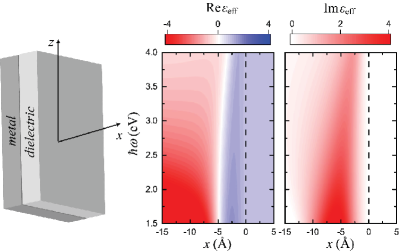
Figure 1: Schematic drawing of a metal-dielectric interface (left-hand panel). Real (middle panel) and imaginary part (right-hand panel) of the effective dielectric function $\varepsilon_{\mathrm{eff}}$ (its component normal to the interface) calculated with GNOR for a Drude metal with $\hbar\omega_{\mathrm{p}}=5$ eV, $\hbar\gamma=0.025$ eV, $v_{\mathrm{F}}=1.07\cdot 10^{6}$ m s^-1, and $D=2\cdot 10^{-4}$ m² s^-1. The dielectric is assumed to be air, described by a dielectric constant equal to one.

The question that still lingers is what expression one should use for $D$. The value $D\propto\beta^{2}/\gamma$ [see equation (17)] was proposed in the original GNOR paper Mortensen:2014 , while an approach based on direct comparison with the broadening predicted by the Kreibig correction was adopted in Raza:2015b . As we showed earlier, equation (17) is consistent with what is expected for diffusive electron transport. However it has yet to be justified in terms of surface dynamics, and must therefore be examined in more detail. In the following we show that the diffusion constant can be related to the dissipative part of the induced surface charge via the Feibelman parameter $d_{\perp}$ Feibelman:1982 . A similar connection to the Feibelman parameters has been presented for the estimation of the resonance energy in Raza:2015b .

Before resorting to the centroid of the induced charge, as introduced by the Feibelman formalism, it is intuitive to consider a simpler approach based on the general, wavevector $\mathbf{q}$-dependent Lindhard dielectric function Lindhard:1954

$$\varepsilon(\omega,\mathbf{q})=\varepsilon_{\mathrm{b}}+\frac{3\omega_{\mathrm{p}}^{2}}{q^{2}v_{\mathrm{F}}^{2}}\left[1-\frac{\omega}{2qv_{\mathrm{F}}}\ln\frac{\omega+qv_{\mathrm{F}}}{\omega-qv_{\mathrm{F}}}\right]~{}.$$ (24)

We revisit the procedure described by Sun and Khurgin in Bozhevolnyi:2016a , and assume that surface scattering is much more important than collisions in the bulk and the relaxation rate $\gamma$ can be taken entirely due to surface effects. Because Landau damping only affects the field components with $q>q_{0}$, an approximation is needed to capture the effect with an effective relaxation time. From the imaginary part of the Drude expression one can relate the relaxation time to the imaginary part of the dielectric function, $\mathrm{Im}\,\varepsilon$, to obtain

$$\gamma=\frac{\omega^{3}\mathrm{Im}\,\varepsilon}{\omega_{\mathrm{p}}^{2}}~{}.$$ (25)

The longitudinal components of the electric field with $q>q_{0}$ will experience Landau damping. To eliminate the $q$-dependence of the Lindhard dielectric function, an effective dielectric function is now defined through

$$\varepsilon_{\mathrm{eff}}(\omega)=\frac{\int_{q_{0}}^{\infty}\mathrm{d}^{3}q\,\varepsilon(\omega,\mathbf{q})\left|E_{\parallel}(\mathbf{q},\omega)\right|^{2}}{\int_{0}^{\infty}\mathrm{d}^{3}q\,\left|E(\mathbf{q},\omega)\right|^{2}}~{}.$$ (26)

The Lindhard dielectric function has a finite imaginary part for $q>q_{0}$ given as

$$\mathrm{Im}\,\varepsilon=\frac{3\omega_{\mathrm{p}}^{2}}{2\omega^{2}q^{3}}~{}.$$ (27)

Assuming again the simple metal-dielectric interface of Fig. 1, a propagating surface plasmon is considered, whose electric field inside the metal is given by $E(x,z)=E_{0}\exp(-x/d_{\mathrm{s}})\exp(\mathrm{i}kz)$, where $d_{\mathrm{s}}$ is the skin depth of the metal. For a typical value of $v_{\mathrm{F}}\sim 10^{6}$ m s^-1 and $d_{\mathrm{s}}\sim 10^{-8}$ m, we then obtain the following effective relaxation rate due to the surface damping

$$\gamma=\frac{3v_{\mathrm{F}}}{4d_{\mathrm{s}}}\sim 10^{14}\,\mathrm{s}^{-1}\;\;\Leftrightarrow\;\;\hbar\gamma\sim 0.414\,\mathrm{eV}~{}.$$ (28)

In nanostructures where one of the characteristic lengths is smaller that the skin depth of the metal, $d_{\mathrm{s}}$ should of course be replaced by this length.

Let us now turn to the more microscopic Feibelman approach Feibelman:1982 ; Christensen:2017 ; Goncalves:2020 , and relate the induced surface charge to the resonance broadening. The Feibelman $d$ parameters have been recently proven an efficient route towards quantum plasmonics Yang:2019 ; Goncalves:2020 , as they are capable of capturing all screening, Landau damping, and spill-out, which are the dominant effects any quantum-informed model should be able to address Tserkezis:2018 . Christensen et al. Christensen:2017 ; Goncalves:2020 have shown that the first-order correction to the damping rate can be connected to the imaginary part of the perpendicular $d$ parameter, $d_{\perp}$, which physically represents the centroid of induced charge, through

$$\gamma^{(1)}=-\frac{1}{4}\frac{\omega_{\mathrm{p}}^{2}}{\omega^{(0)}}\Lambda_{\perp}\mathrm{Im}\,d_{\perp}^{(0)}~{},$$ (29)

where $\Lambda_{\perp}$ is a geometric parameter, and the superscript ${(0)}$ indicates that the corresponding function is to be calculated on resonance. For the dipole resonance in a sphere, $\omega^{(0)}\simeq\omega_{\mathrm{p}}/\sqrt{3}$, and the correction to the damping rate becomes

$$\gamma^{(1)}=\frac{1}{3R}\frac{\omega_{\mathrm{p}}^{2}}{\omega^{(0)}}\mathrm{Im}\,d_{\perp}^{(0)}~{}.$$ (30)

Comparing with the GNOR expression of equation (22) one can obtain a first approximate connection between the diffusion constant and the induced surface charge:

$$D=\frac{8\beta}{\sqrt{2}}\mathrm{Im}\,d_{\perp}^{(0)}.$$ (31)

In Fig. 2 we plot with dotted lines the complex hydrodynamic parameter $\eta^{2}$ obtained based on equation (7), for the diffusion constant derived from equation (31), using the Feibelman parameter derived in Christensen:2017 for a jellium metal with Wigner–Seitz radius $r_{\mathrm{s}}=4$, which well represents Na. The plasma frequency corresponding to this radius is $\hbar\omega_{\mathrm{p}}=5.89143$   eV, and the Fermi velocity is $v_{\mathrm{F}}=1.07\cdot 10^{6}$ m s^-1, while for the Drude damping rate we assume $\hbar\gamma=0.1$   eV. We note here that we focus on Na, even though hydrodynamics is known to fail to predict the correct frequency shifts in its case – as will be shown in Fig. 3 – because Feibelman parameters have only been unambiguously derived for jellium metals. Obtaining such parameters for noble metals is a more challenging task, and constitutes part of our ongoing activities.

The $D$ obtained from equation (31) can be a good starting point for using the GNOR model. Most notably, it turns out that it is in very good agreement with the corresponding results obtained assuming a constant diffusion constant $D$ chosen to match the damping of the SDB model Raza:2015a (dashed lines in Fig. 2). Nevertheless, it is still derived based on just the dipolar mode of a spherical nanoparticle, and extending its use to different shapes or even higher-order modes of spheres is not straightforward to justify, as it assumes that the damping is the same in all cases and all frequencies. A more general, frequency-dependent approach, which only disregards curvature effects, could be based on the reflection coefficients of a flat metal-dielectric interface. In the $d$-parameter formalism, the reflection coefficient for $p$ polarisation is given by Feibelman:1982 ; Goncalves:2020

$$r_{d_{\perp},p}=$$

$$\frac{\varepsilon_{\mathrm{m}}k_{x,\mathrm{d}}-\varepsilon_{\mathrm{d}}k_{x,\mathrm{m}}+\left(\varepsilon_{\mathrm{m}}-\varepsilon_{\mathrm{d}}\right)\left[\mathrm{i}q^{2}d_{\perp}-\mathrm{i}k_{x,\mathrm{d}}k_{x,\mathrm{m}}d_{\parallel}\right]}{\varepsilon_{\mathrm{m}}k_{x,\mathrm{d}}+\varepsilon_{\mathrm{d}}k_{x,\mathrm{m}}-\left(\varepsilon_{\mathrm{m}}-\varepsilon_{\mathrm{d}}\right)\left[\mathrm{i}q^{2}d_{\perp}+\mathrm{i}k_{x,\mathrm{d}}k_{x,\mathrm{m}}d_{\parallel}\right]},$$

where $d_{\parallel}$ is the parallel $d$ parameter (centroid of induced current), $q$ is now the in-plane wavenumber and $k_{j}=\sqrt{\varepsilon_{j}}k_{0}$ is the bulk wavenumber, with $j=\mathrm{d},\mathrm{m}$ denoting the medium, dielectric or metal, and $k_{0}=\omega/c$ is the free-space wavenumber; $\varepsilon_{j}$ is the (complex and dispersive, but local) permittivity of medium $j$, and $k_{x,j}=\sqrt{k_{j}^{2}-q^{2}}$ is the wavenumber in the out-of-plane direction, taken to be the $x$ direction (see Fig. 1). On the other hand, in a generalised hydrodynamic formalism, the corresponding reflection coefficient reads David:2013

$$r_{h,p}=\frac{\varepsilon_{\mathrm{m}}k_{x,\mathrm{d}}-\varepsilon_{\mathrm{d}}k_{x,\mathrm{m}}\left(1+\delta_{h}\right)}{\varepsilon_{\mathrm{m}}k_{x,\mathrm{d}}+\varepsilon_{\mathrm{d}}k_{x,\mathrm{m}}\left(1+\delta_{h}\right)}~{},$$ (33)

with $\delta_{h}=[q^{2}(\varepsilon_{\infty}-\varepsilon_{\mathrm{m}})]/(k_{x,\mathrm{m}}k_{x,\mathrm{nl}}\varepsilon_{\infty})$ and $k_{x,\mathrm{nl}}^{2}=k_{\mathrm{nl}}^{2}-q^{2}=[\omega(\omega+\mathrm{i}\gamma)-\omega_{\mathrm{p}}^{2}/\varepsilon_{\infty}]/\eta^{2}-q^{2}$. In all cases, the imaginary part of $k_{x}$ must be larger than zero, to ensure a passive medium. Direct comparison between Eqs. (V) and (33) in the long-wavelength limit ($q\rightarrow 0$) yields PrivateCommun

$$d_{\perp}=-\frac{\mathrm{i}}{k_{\mathrm{nl}}}\frac{\varepsilon_{\mathrm{d}}}{\varepsilon_{\infty}}\frac{\varepsilon_{\mathrm{m}}-\varepsilon_{\infty}}{\varepsilon_{\mathrm{m}}-\varepsilon_{\mathrm{d}}}~{}.$$ (34)

Solving for $\eta^{2}$, with the constraints that $\mathrm{Im}\,k_{\mathrm{nl}}$ should be positive Feibelman:1982 and the imaginary part of $\eta^{2}$, as introduced in GNOR Mortensen:2014 needs to be negative to ensure a lossy medium, one can obtain a quantum-informed, generalised dispersive expression for the complex convective-diffusive hydrodynamic parameter, which can apply equally well to all shapes of nanostructures wiener_nl12 . In Fig. 2 this $\eta^{2}$ is plotted as a function of frequency with solid lines.

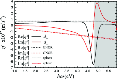
Figure 2: Complex convective-diffusive hydrodynamic parameter $\eta^{2}$ (real part: black lines; imaginary part: red lines), as obtained by the $d_{\perp}$ method [equation (34)] from the reflection coefficient of a flat air-Na interface (solid lines), from the GNOR diffusion constant obtained from $d_{\perp}$ for a sphere through equation (31) (dotted lines), or for a constant diffusion parameter $D=2.67\cdot 10^{-4}$  m² s^-1 Raza:2015a (dashed lines). In all cases, we have assumed a jellium metal with $r_{\mathrm{s}}=4$ and $\hbar\omega_{\mathrm{p}}=$ 5.89143 eV, $\hbar\gamma=$ 0.1 eV, $v_{\mathrm{F}}=1.07\cdot 10^{6}$ m s^-1). The Feibelman $d_{\perp}$ parameter is obtained from Christensen:2017 . The shaded area denotes the frequency range (around the Bennett resonance, and close to the plasma frequency) where a calculation of $\eta^{2}$ based on equation (34) is ambiguous and cannot be trusted.

Up to around 4.7 eV the results obtained through equation (34) are close to those corresponding to constant diffusion parameters, predicting a slightly lower damping in the low-frequency limit. This behaviour is maintained as the frequency increases, and one approaches the region of interest, where all plasmonic resonances are expected (the dipolar resonance of a Na sphere in the quasistatic limit is around 3.4 eV). For even higher frequencies, however, the $d$ parameter-based $\eta^{2}$ becomes more ambiguous, especially around the so-called Bennett multipole surface plasmon Toscano:2015 ; Bennett:1970 which appears due to spill-out at 4.7 eV. In this region, and all the way up to the plasma frequency (grey-shaded area in Fig. 2), the requirement that the imaginary part of the retrieved $\eta^{2}$ be negative leads to both real and imaginary part appearing with the opposite sign of what is shown in the figure. In that case, instead of the typical shape of a Lorentzian around a resonance, one would get an unnatural, kinked curve, which obviously violates the Kramers–Kronig relations Ashcroft:1976 . So one of the two requirements has to be relaxed, and since Kramers–Kronig relations are a manifestation of causality, we choose to comply with them. Doing this, the retrieval process is forced to introduce a fictitious gain, in agreement with the local equivalent-layer approach of luo_prl111 [note that when co-existing with the even more lossy response of the bulk, it still results in a net lossy response, see equation (6)]. Obviously, asking a hydrodynamic description of the bulk, with spill-in intrinsically built into it, to reproduce all the physics captured by a surface-response function which predicts spill-out has its limitations, and the results in the grey-shaded area cannot be trusted. Our approach has, nevertheless, provided a link between other phenomenological approaches to quantify surface-enhanced Landau damping, and they all appear consistent up to $\simeq 0.8\omega_{\mathrm{p}}$.

VI Numerical results

To illustrate the predictions of our analysis and the value of the $d$ parameter-based calculation of $\eta^{2}$, we present in Fig. 3 analytic calculations of normalised extinction cross section spectra for a Na sphere described by a Drude model with the parameters mentioned at the end of Sec. V. The radius of the sphere is taken equal to $R=5$ nm, and the spectra are calculated with an implementation of GNOR based on Mie theory Tserkezis:2016a , using either the hydrodynamic parameter obtained by equation (7) (dark-blue shaded line) or the constant diffusion parameter $D$ suggested in Raza:2015a (green open circles). The results are compared to those of LRA (red line), together with the standard HDM (light blue line) and the SDB phenomenological correction (dark-red shaded line, with $A=1.0$). The spectrum obtained by calculating $\eta^{2}$ using the Feibelman-based recipe outlined above agrees very well in resonant frequency with the prediction of HDM, and gives slightly smaller broadening as compared to SDB (whose constant $A$ contains a certain arbitrariness anyway). The open green circles already show that the effect of the surface-enhanced Landau damping can in principle be captured using a constant GNOR diffusion term, but the full connection to the centroid of induced charge can be more accurate, as it contains the quantum-mechanically calculated frequency dependence of the hydrodynamic parameters.

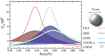
Figure 3: Normalised extinction cross section for a Na sphere with radius $R=5$ nm, as obtained within LRA (red line), SDB (dark-red shaded line), HDM (light blue line), GNOR with a $d_{\perp}$-based hydrodynamic parameter (dark-blue shaded line) and GNOR with a constant diffusion $D=2.67\cdot 10^{-4}$  m² s^-1 (open green circles).

As further demonstration of the potential of our derivation, we study in Fig. 4 two nanoparticles of different shapes: a cylinder with diameter $R/2$ and height $H$ both equal to 10 nm (a), and a cube with side $a=$ 10 nm (b). The spectra are obtained using our implementation of hydrodynamic methods to a commercial finite-element solver (Comsol Multiphysics 5.1), with the only change compared to previous studies Tserkezis:2018 ; Tserkezis:2016a ; Tserkezis:2017 being the calculation of $\eta^{2}$, which is now performed not based on Eq. (7) for constant $\beta$ and $D$, but by solving Eq. (34) for the $d_{\perp}$ values obtained from Christensen:2017 (as interpolated by an analytic function in Goncalves:2020 ). The NPs were modelled with approximately $100000$ tetrahedral domain elements with minimum side of $0.2$ nm, while perfectly-matched layers of thickness $300$ nm were used to minimise reflections at the simulation area boundaries. The results are again compared both to the LRA approximation and the traditional GNOR approach with constant diffusion. In both cases, it is evident that the constant-$D$ results overestimate both the damping and the blueshift of the modes, a response which could be anticipated by the differences between the corresponding $\eta^{2}$ values in Fig. 2, especially in the region of higher order (edge or corner) modes Grillet:2011 , which are always affected more by damping.

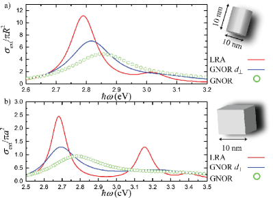
Figure 4: (a) Normalised extinction cross section spectra for a cylinder with diameter $R/2=10$ nm and height $H=10$ nm, as obtained within LRA (red line), GNOR with a $d_{\perp}$-based hydrodynamic parameter (dark blue line), and GNOR with constant diffusion $D=2.67\cdot 10^{-4}$  m² s^-1 (green open circles). The incident field is polarised at an angle $\theta=30^{\circ}$ with respect to the cylinder axis. (b) Same as (a), for a cube with side $a=10$ nm. The incident field is polarised along one of the cube sides.

The above analysis and results clearly display the main strength of the Feibelman-based approach: because $d_{\perp}$ is obtained for a planar interface, one quantum-mechanical (e.g. with density-functional theory) calculation per material should be sufficient to obtain the hydrodynamic parameter $\eta^{2}$, which can subsequently be introduced to hydrodynamic calculations in arbitrary geometries, as already implemented in a series of different numerical McMahon:2010a ; Toscano:2012 ; Trugler:2017 ; Li:2017 ; Doicu:2020 or approximate methods luo_prl111 . In addition to being easily generalisable, the results presented in this article also establish a solid link between the surface-enhanced Landau damping and the electron convection-diffusion mechanisms, thus providing a theoretical justification of the introduction of the GNOR diffusion term.

VII Conclusion

We have discussed the origin and role of the diffusion term included in the GNOR theory for nonlocal plasmonics. Based on the Boltzmann equation, we showed that the diffusion-induced damping in GNOR cannot have its origins in the bulk of the material, but should be considered as an efficient way to capture surface-enhanced Landau damping. We linked the complex hydrodynamic convection-diffusion parameter to the induced surface charge via the Feibelman $d_{\perp}$ parameter for the centroid of induced charge, enabling the extraction of the input required for hydrodynamic models from systematic ab-initio calculations. The results obtained for a single metal-dielectric interface can be implemented in any geometry, thus allowing to expand the use of GNOR in a wide range of applications in nonclassical plasmonics.

References

References

- (1) Tame M S, McEnery K R, Özdemir Ş K, Lee J, Maier S A and Kim M S Nature Phys. 2013 9 329–340
- (2) Bozhevolnyi S I, Martín-Moreno L and García-Vidal F J 2017 Quantum Plasmonics (Springer)
- (3) Bozhevolnyi S I and Mortensen N A Nanophotonics 2017 6 1185–1188
- (4) Zhu W, Esteban R, Borisov A G, Baumberg J J, Nordlander P, Lezec H J, Aizpurua J and Crozier K B Nature Commun. 2016 7 11495
- (5) Fitzgerald J M, Narang P, Craster R V, Maier S A and Giannini V Proc. IEEE 2016 104 2307–2322
- (6) Yannopapas V Int. J. Mod. Phys. B 2017, 31 1740001
- (7) Amendola V, Pilot R, Frasconi M, Maragò O M and Iatì M A J. Phys.: Condens. Matter 2017 29 203002
- (8) Fernández-Domínguez A I, Bozhevolnyi S I and Mortensen N A ACS Photonics 2018 5 3447
- (9) Ciracì C, Jurga R, Khalid M and Della Sala F Nanophotonics 2019 6 1821–1833
- (10) Savage K J, Hawkeye M M, Esteban R, Borisov A G, Aizpurua J and Baumberg J J Nature 2012, 491 574–577
- (11) Duan H, Fernández-Domínguez A I, Bosman M, Maier S A and Yang J K W Nano Lett. 2012, 12 1683–1689
- (12) Scholl J A, Koh A L and Dionne J A Nature 2012, 483 421–427
- (13) Scholl J A, García-Etxarri A, Koh A L and Dionne J A Nano Lett. 2013 13 564–569
- (14) Wiener A, Duan H, Bosman M, Horsfield A P, Pendry J B, Yang J K W, Maier S A and Fernández-Domínguez A I ACS Nano 2013 7 6287–6296
- (15) Jung H, Cha H, Lee D and Yoon S ACS Nano 2015 9 12292–12300
- (16) Raza S, Kadkhodazadeh S, Christensen T, Di Vece M, Wubs M, Mortensen N A and Stenger N, Nature Commun. 2015 6 8788
- (17) Krasavin A V, Ginzburg P, Wurtz G A and Zayats A V Nature Commun. 2016 7 11497
- (18) Shen H, Chen L, Ferrari L, Lin M-H, Mortensen N A, Gwo S and Liu Z, Nano Lett. 2017 17 2234–2239
- (19) García de Abajo F J J. Phys. Chem. C 2008112 17983–17987
- (20) McMahon J M, Gray S K and Schatz G C Nano Lett. 2010 10 3473–3481
- (21) Raza S, Toscano G, Jauho A-P, Wubs M and Mortensen N A Phys. Rev. B 2011 84 121412(R)
- (22) Ciracì C, Hill R T, Mock J J, Urzhumov Y, Fernández-Domínguez A I, Maier S A, Pendry J B, Chilkoti A and Smith D R Science 2012 337 1072–1074
- (23) David C and García de Abajo F J ACS Nano 2014 8 9558–9566
- (24) Christensen T, Yan W, Raza S, Jauho A-P, Mortensen N A and Wubs M ACS Nano 2014 8 1745–1758
- (25) Raza S, Bozhevolnyi S I, Wubs M and Mortensen N A J. Phys.: Condens. Matter 2015 27 183204
- (26) Eremin Y, Doicu A and Wriedt T J. Quant. Spectr. Rad. Transf. 2018 217 35–44
- (27) Kupresak M, Zheng X, Vandenbosch G A E andMoshchalkov V V Adv. Theory Simul. 2020 3 1900172
- (28) Esteban R, Borisov A G, Nordlander P and Aizpurua J Nature Commun. 2012 3 825
- (29) Stella L, Zhang P, García-Vidal F J, Rubio A and García-González P J. Phys. Chem. C 2013 117 8941–8949
- (30) Teperik T V, Nordlander P, Aizpurua J and Borisov A G Phys. Rev. Lett. 2013 110 263901
- (31) Yan W, Wubs M and Mortensen N A Phys. Rev. Lett. 2015 115 137403
- (32) Hohenester U and Draxl C Phys. Rev. B 2016 94 165418
- (33) Toscano G, Straubel J, Kwiatkowski A, Rockstuhl C, Evers F, Xu H, Mortensen N A and Wubs M Nature Commun. 2015 6 7132
- (34) Yan W Phys. Rev. B 2015 91 115416
- (35) Ciracì C and Della Sala F Phys. Rev. B 2016 93 205405
- (36) Raza S, Stenger N, Kadkhodazadeh S, Fischer S V, Kostesha N, Jauho A-P, Burrows A, Wubs M and Mortensen N A Nanophotonics 2013 2 131–138
- (37) Kreibig U and Zacharias P Z. Physik 1970 231 128–143
- (38) Kraus W A and Schatz G C J. Chem. Phys. 1983 79 6130–6139
- (39) Kubo R Rep. Prog. Phys. 1966 29 255
- (40) Mortensen N A, Raza S, Wubs M, Søndergaard T and Bozhevolnyi S I Nature Commun. 2014 5 3809
- (41) Apell P, Monreal R and Flores F Solid State Commun. 1984 52 971–973
- (42) Ouyang F, Batson P E and Isaacson M Phys. Rev. B 1992 46 15421–15425
- (43) Baida H, Billaud P, Marhaba S, Christofilos D, Cottancin E, Crut A, Lermé J, Maioli P, Pellarin M, Broyer M, Del Fatti N, Vallée F, Sánchez-Iglesias A, Pastoriza-Santos I and Liz-Marzán L M Nano Lett. 2009 9 3463–3469
- (44) Lermé J, Baida H, Bonnet C, Broyer M, Cottancin E, Crut A, Maioli P, Del Fatti N, Vallée F and Pellarin M J. Phys. Chem. Lett. 2010 1, 2922–2928
- (45) Monreal R C, Antosiewicz T J and Apell S P New J. Phys. 2013 15 083044
- (46) Li X, Xiao D and Zhang Z New J. Phys. 2013 15 023011
- (47) Khurgin J B Faraday Discuss. 2015 178 109–122
- (48) Uskov A V, Protsenko I E, Mortensen N A and O’Reilly E P Plasmonics 2014 9 185–192
- (49) Kirakosyan A S, Stockman M I and Shahbazyan T V Phys. Rev. B 2016 94 155429
- (50) Shahbazyan T V Phys. Rev. B 2016 94 235431
- (51) Lermé J, Bonnet C, Lebeault M-A, Pellarin M and Cottancin E J. Phys. Chem. C 2017 121 5693–5708
- (52) Chandrasekhar S Rev. Mod. Phys. 1943 15 1–89
- (53) Landau L D, Lifshitz E M and Pitaevskii L P 1984 Electrodynamics of Continuous Media (Butterworth Heinemann)
- (54) Hanson G W IEEE Anten. Propag. Mag. 2010 52 198–207
- (55) Iwamoto N, Krotscheck E and Pines D Phys. Rev. B 1984 29 3936–3951
- (56) Feibelman P J Prog. Surf. Sci. 1982 12 287–408
- (57) Kreibig U and Genzel L Surf. Sci. 1985 156 678–700
- (58) Boardman A D 1982 Electromagnetic Surface Modes (Wiley)
- (59) Tokatly I and Pankratov O Phys. Rev. B 1999 60 15550–15553
- (60) Halevi P Phys. Rev. B 1995 51 7497–7499
- (61) Luo Y, Fernandez-Dominguez A I, Wiener A, Maier S A and Pendry J B 2013 Phys. Rev. Lett. 111 093901
- (62) Ashcroft N W and Mermin N D 1976 Solid State Physics (Harcourt)
- (63) Campos A, Troc N, Cottancin E, Pellarin M, Weissker H-C, Lermé J, Kociak M and Hillenkamp M Nature Phys 2019 15 275–280
- (64) Rammer J and Smith H Rev. Mod. Phys. 1986 58 323–359
- (65) Wubs M and Mortensen N A Springer Series in Solid-State Sciences 2016 185 279–302
- (66) Tserkezis C, Yan W, Hsieh W, Sun G, Khurgin J B, Wubs M and Mortensen N A Int. J. Mod. Phys. B 2017 31 1740005
- (67) Raza S, Wubs M, Bozhevolnyi S I and Mortensen N A Opt. Lett. 2015 40 839–842
- (68) Lindhard J Dan. Mat. Fys. Medd. 1954 28 1–57
- (69) Yang Y, Zhu D, Yan W, Agarwal A, Zheng M, Joannopoulos J D, Lalanne P, Christensen T, Berggren K K and Soljačić M Nature 2019 576 248–252
- (70) Gonçalves, P A D, Christensen, T, Rivera N, Jauho A-P, Mortensen N A and Soljačić M Nature Commun. 2020 11 366
- (71) Tserkezis C, Yeşilyurt A T M, Huang J-S and Mortensen N A ACS Photonics 2018 5 5017–5024
- (72) Christensen T, Yan W, Jauho A-P, Soljačić M and Mortensen N A Phys. Rev. Lett. 2017 118 157402
- (73) David C, Mortensen N A and Christensen J Sci. Rep. 2013 3 2526
- (74) Gonçalves, P A D Private communication. 2020.
- (75) Wiener A, Fernández-Domínguez A I, Horsfield A P, Pendry J B and Maier S A 2012 Nano Lett. 12 3308–14
- (76) Bennett A J Phys. Rev. B 1970 1 203–207
- (77) Tserkezis C, Maack J R, Liu Z, Wubs M and Mortensen N A Sci. Rep. 2016 6 28441
- (78) Tserkezis C, Wubs M and Mortensen N A Phys. Rev. B 2017 96 085413
- (79) Grillet N, Manchon D, Bertorelle F, Bonnet C, Broyer M, Cottancin E, Lermé J, Hillenkamp M and Pellarin M ACS Nano 2011 5 9450–9462
- (80) McMahon J M, Gray S K and Schatz G C Phys. Rev. B 2010 82 035423
- (81) Toscano G, Raza S, Jauho A-P, Mortensen N A and Wubs M Opt. Express 2012 20 4176–4188
- (82) Trügler A, Hohenester U and García de Abajo F J Int. J. Mod. Phys. B 2017 31, 1740007
- (83) Li L, Lanteri S, Mortensen N A, and Wubs M Comp. Phys. Commun. 2017 219 99
- (84) Doicu A, Eremin Y and Wriedt T J. Quant. Spectr. Rad. Transf. 2020 242 106756