TSML (Time Series Machine Learning)

Abstract

Over the past years, the industrial sector has seen many innovations brought about by automation. Inherent in this automation is the installation of sensor networks for status monitoring and data collection. One of the major challenges in these data-rich environments is how to extract and exploit information from these large volume of data to detect anomalies, discover patterns to reduce downtimes and manufacturing errors, reduce energy usage, predict faults/failures, effective maintenance schedules, etc. To address these issues, we developed TSML. Its technology is based on using the pipeline of lightweight filters as building blocks to process huge amount of industrial time series data in parallel.

1 Introduction

TSML[tsml2019] is a Julia[bezanson2017julia] package for time series data processing, classification, and prediction. It provides common API for ML (Machine Learning) libraries from Python’s Scikit-Learn, R’s Caret, and native Julia MLs for seamless integration of heterogeneous libraries to create complex ensembles for robust time series prediction, clustering, and classification. TSML has the following features:

1. data type clustering/classification for automatic data discovery

2. aggregation based on date/time interval

3. imputation based on symmetric Nearest Neighbors

4. statistical metrics for data quality assessment and classification input features

5. ML wrapper with more than 100+ libraries from caret, scikit-learn, and julia

6. date/value matrix conversion of 1-D time series using sliding windows to generate features for ML prediction

7. pipeline API for high-level description of the processing workflow

8. specific cleaning/normalization workflow based on data type

9. automatic selection of optimised ML model

10. automatic segmentation of time-series data into matrix form for ML training and prediction

11. extensible architecture using just two main interfaces: fit and transform

12. meta-ensembles for automatic feature and model selection

13. support for distributed/threaded computation for scalability and speed

The TSML package assumes a two-column input for any time series data composed of dates and values. The first part of the workflow aggregates values based on the specified date/time interval which minimizes occurrence of missing values and noise. The aggregated data is then left-joined to the complete sequence of dates in a specified date/time interval. Remaining missing values are replaced by the median/mean or user-defined aggregation function of the k-nearest neighbors (k-NN) where k is the symmetric distance from the location of missing value. This approach can be called several times until there are no more missing values.

For prediction tasks, TSML extracts the date features and convert the value column into matrix form parameterized by the size and stride of the sliding window. The final part joins the date features and the value matrix to serve as input to the ML with the output representing the values of the time periods to be predicted ahead of time.

TSML uses a pipeline which iteratively calls the fit! and transform! families of functions relying on multiple dispatch to dynamically select the correct algorithm from the steps outlined above. Machine learning functions in TSML are wrappers to the corresponding Scikit-Learn, Caret, and native Julia ML libraries. There are more than hundreds of classifiers and regression functions available using TSML’s common API.

2 TSML Workflow

All major data processing types in TSML are subtypes of the Transformer. There are two major types of transformers, namely: filters for data processing and learners for machine learning. Both transformers implement the fit! and transform! multi-dispatch functions. All filters are direct subtypes of the Transformer while all learners are subtypes of the TSLearner. The TSLearner is a direct subtype of the Transformer.

Filters are normally used for pre-processing tasks such as imputation, normalization, feature extraction, feature transformation, scaling, etc. Consequently, filters’ fit! and transform! functions expect one argument which represents an input data for feature extraction or transformation. Each data type must implement fit! and transform! although in some cases, only transform! operation is needed. For instance, square root or log filters do not require any initial computation of parameters to transform their inputs. On the other hand, feature transformations such as scaling, normalization, PCA, ICA, etc. require initial computation of certain parameters in their input before applying the transformation to new datasets. In these cases, initial computations of these parameters are performed by the fit! function while their applications to new datasets are done by the transform! function.

Learners, on the other hand, expect two arguments (input vs output) and require training cycle to optimize their parameters for optimal input–output mapping. The training part is handled by the fit! function while the prediction part is handled by the transform! function.

The TSML workflow borrows the idea of the Unix pipeline[orchestra2014, combineml2016]. The Pipeline data type is also a subtype of the Transformer and expects two arguments: input and output. The main elements in a TSML pipeline are series of transformers with each performing one specific task and does it well. The series of filters are used to perform pre-processing of the input while a machine learner at the end of the pipeline is used to learn the input–output mapping. From the perspective of using the Pipeline where the last component is a machine learner, the fit! function is the training phase while the transform! function is the prediction or classification phase.

The fit! function in the Pipeline iteratively calls the fit! and transform! functions in a series of transformers. If the last transformer in the pipeline is a learner, the last transformed output from a series of filters will be used as input features for the fit! or training phase of the said learner.

During the prediction task, the transform! function in the Pipeline iteratively calls the transform! operations in each filter and learner. The transform operation is direct application of the parameters computed during normalization, scaling, training, etc. to the new data. If the last element in the pipeline during transform is a learner, it performs prediction or classification. Otherwise, the transform operation acts as a feature extractor if they are composed of filters only.

To illustrate, below describes the main steps in using the TSML. First, we create filters for csv reading, aggregation, imputation, and data quality assessment.

[language = Julia] fname = joinpath(dirname(pathof(TSML)), "../data/testdata.csv") csvfilter = CSVDateValReader(Dict( :filename=>fname, :dateformat=>"dd/mm/yyyy HH:MM")) valgator = DateValgator(Dict( :dateinterval=>Dates.Hour(1))) valnner = DateValNNer(Dict( :dateinterval=>Dates.Hour(1))) stfier = Statifier(Dict(:processmissing=>true))

We can then setup a pipeline containing these filters to process the csv data by aggregating the time series hourly and check the data quality using the Statifier filter (Fig. 1).

[language = Julia] apipeline = Pipeline(Dict( :transformers => [csvfilter, valgator, stfier])) fit!(apipeline) mystats = transform!(apipeline) @show mystats

Figure 1: Data Quality Statistics. Column names starting with ‘b‘ refer to statistics of contiguous blocks of missing data.

A mentioned previously, the fit! and transform! in the pipeline iteratively calls the corresponding fit! and transform! within each filter. This common API relying on Julia’s multi-dispatch mechanism greatly simplifies the implementations, operations, and understanding of the entire workflow. In addition, extending TSML functionality is just a matter of creating a new data type filter and define its own fit! and transform! functions.

In the Statifier filter result, blocks of missing data is indicated by column names starting with b. Running the code indicates that there are plenty of missing data blocks. We can add the ValNNer filter to perform k-nearest neighbour (k-NN) imputation and check the statistics (Fig. 2):

[language = Julia] bpipeline = Pipeline(Dict( :transformers => [csvfilter, valgator, valnner,stfier])) fit!(bpipeline) imputed = transform!(bpipeline) @show imputed

Figure 2: Statistics after Imputation. All statistics for blocks of missing data indicate NaN to indicate the stats of empty set. This implies that all missing blocks are imputed.

The result in Fig. 2 indicates NaN for all missing data statistics column because the set of missing blocks count is now empty.

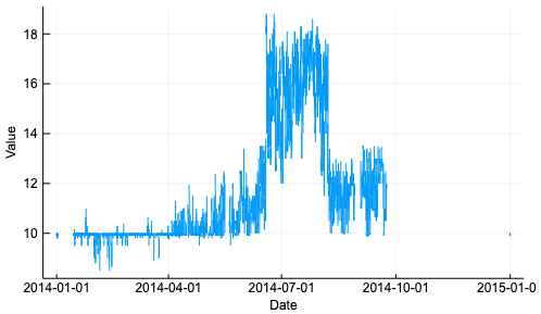
We can also visualise our time series data using the Plotter filter instead of the Statifier as shown in Fig 3. Looking closely, you will see discontinuities in the plot due to blocks of missing data.

[language = Julia] pltr=Plotter(Dict(:interactive => true)) plpipeline = Pipeline(Dict( :transformers => [csvfilter, valgator, pltr])) fit!(plpipeline) transform!(plpipeline)

Figure 3: Plot with Missing Data

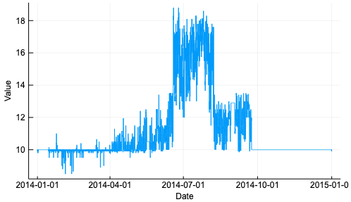
Using the imputation pipeline described before, we can visualise the result by replacing the Statifier with the Plotter filter. Figure 4 shows the plot after imputation which gets rid of missing data.

[language = Julia] bplpipeline = Pipeline(Dict( :transformers => [csvfilter, valgator, valnner,pltr])) fit!(bplpipeline) transform!(bplpipeline)

Figure 4: Plot after Data Imputation

2.1 Processing Monotonic Time Series

This subsection dicusses additional filters to handle monotonic data which are commonly employed in energy/water meter and footfall sensors. In the former case, the time series type is strictly monotonically increasing while in the latter case, the monotonicity happens daily. We use the filter called Monotonicer which automatically detects these two types of monotonic sensors and apply the normalisation accordingly.

[language = Julia] mono = joinpath(dirname(pathof(TSML)), "../data/typedetection/monotonic.csv") monocsv = CSVDateValReader(Dict(:filename=>mono, :dateformat=>"dd/mm/yyyy HH:MM"))

Let us plot in Fig. 5 the monotonic data with the usual workflow of aggregating and imputing the data first.

[language = Julia] monopipeline = Pipeline(Dict( :transformers => [monofilecsv,valgator, valnner,pltr])) fit!(monopipeline) transform!(monopipeline)

Figure 5: Monotonic Time Series

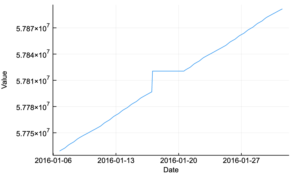
Let us now normalise using Monotonicer and show the plot in Fig. 6.

[language = Julia] mononicer = Monotonicer(Dict()) monopipeline = Pipeline(Dict( :transformers => [monofilecsv,valgator,valnner, mononicer, pltr])) fit!(monopipeline) transform!(monopipeline)

Figure 6: Normalized Monotonic Time Series

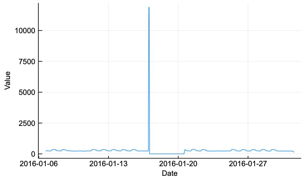
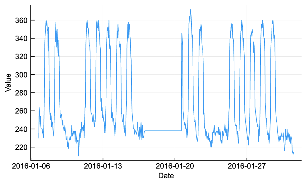
The presence of outlier due to some random errors during meter reading becomes obvious after the normalisation. To remedy this issue, we add the Outliernicer filter which detects outliers and replace them using the k-NN imputation technique used by the DateValNNer filter (Fig. 7).

[language = Julia] outliernicer = Outliernicer( Dict(:dateinterval=>Dates.Hour(1))) monopipeline = Pipeline(Dict( :transformers => [monofilecsv,valgator,valnner, mononicer,outliernicer,pltr])) fit!(monopipeline) transform!(monopipeline)

Figure 7: Normalized Monotonic Time Series With Outlier Removal Filter

2.2 Processing Daily Monotonic Time Series

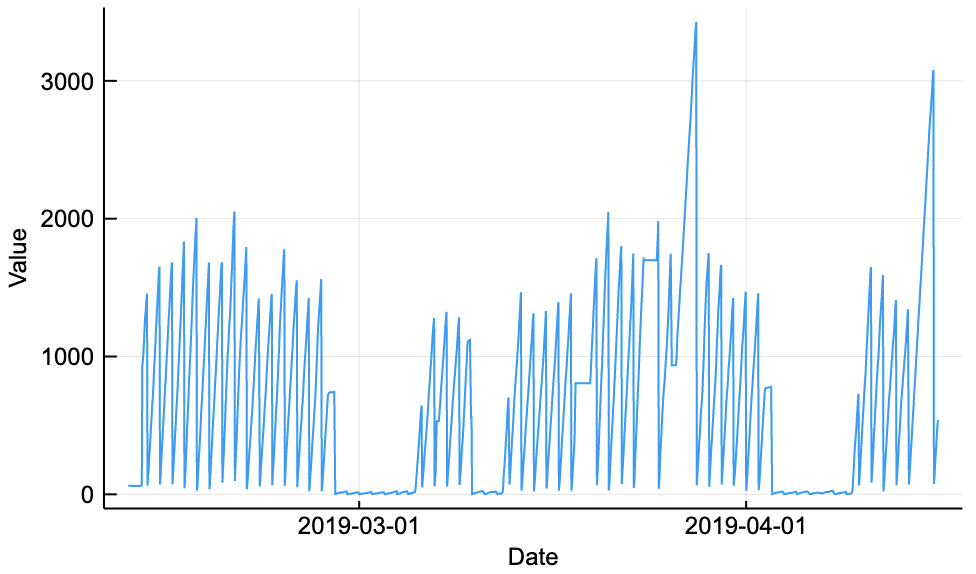
We follow similar workflow in the previous subsection to normalize daily monotonic time series. First, let us visualize the original data after aggregation and imputation (Fig. 8).

[language = Julia] dailymono = joinpath(dirname(pathof(TSML)), "../data/type-detection/dailymonotonic.csv") dailymonocsv = CSVDateValReader(Dict( :filename=>dailymono, :dateformat=>"dd/mm/yyyy HH:MM")) dailymonopipeline = Pipeline(Dict( :transformers => [dailymonocsv,valgator, valnner,pltr])) fit!(dailymonopipeline) transform!(dailymonopipeline)

Figure 8: Daily Monotonic Time Series

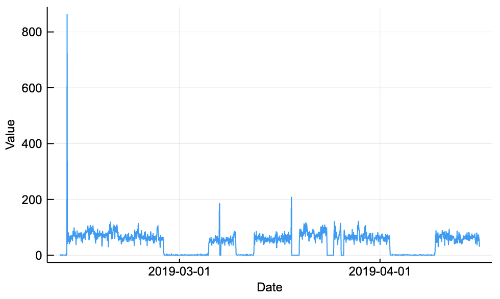
Then, we reuse the Monotonicer filter in the previous subsection to normalise the data and plot (Fig. 9).

[language = Julia] dailymonopipeline = Pipeline(Dict( :transformers => [dailymonocsv,valgator, valnner,mononicer,pltr])) fit!(dailymonopipeline) transform!(dailymonopipeline)

Figure 9: Normalized Daily Monotonic Time Series

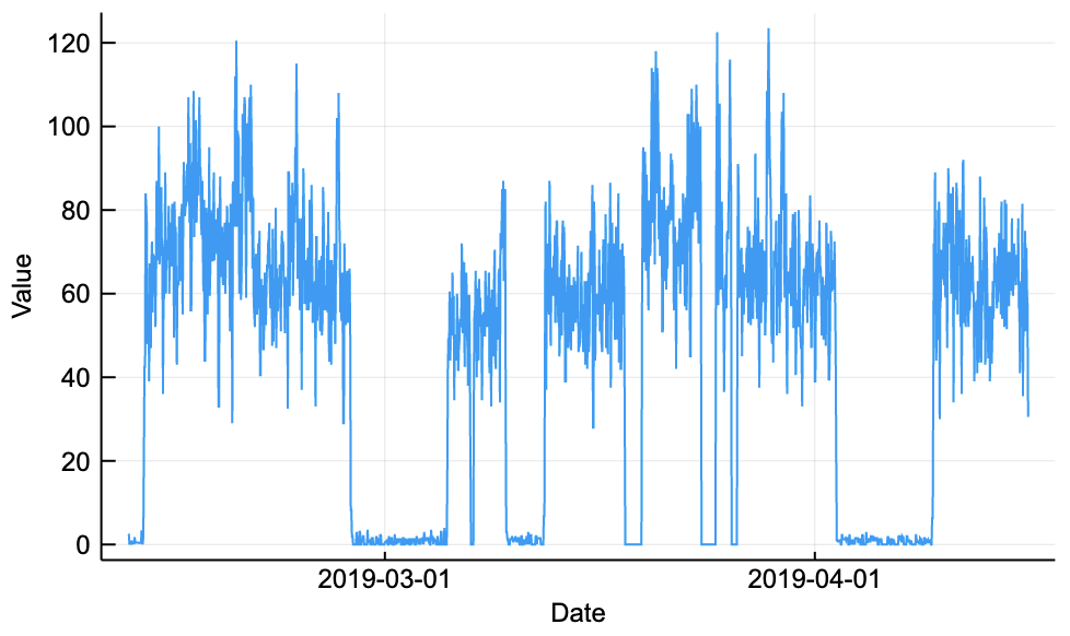
To remove outliers, we can reuse the Outliernicer filter in the previous subsection and plot the cleaned data (Fig. 10).

[language = Julia] dailymonopipeline = Pipeline(Dict( :transformers=>[dailymonocsv,valgator,valnner, mononicer,outliernicer,pltr])) fit!(dailymonopipeline) transform!(dailymonopipeline)

Figure 10: Normalized Daily Monotonic Time Series with Outlier Detector

3 Time Series Classification

We can use the knowledge we learned in setting up the TSML pipeline containing filters and machine learners to build higher level operations to solve a specific industrial problem. One major problem which we consider relevant because it is a common issue in IOT (Internet of Things) is the time series classification. This problem is prevalent nowadays due to the increasing need to use many sensors to monitor status in different aspects of industrial operations and maintenance of cars, buildings, hospitals, supermarkets, homes, and cities.

Rapid deployment of these sensors result to many of them not properly labeled or classified. Time series classification is a significant first step for optimal prediction and anomaly detection. Identifying the correct sensor data types can help in the choice of what the most optimal prediction model to use for actuation or pre-emption to minimise wastage in resource utilisation. To successfully perform the latter operations, it is necessary to identify first the time series type so that appropriate model and cleaning routines can be selected for optimal model performance. The TSClassifier filter aims to address this problem and its usage is described below.

First, we setup the locations of files for training, testing, and saving the model. Next, we start the training phase by calling fit! which loads file in the training directory and learn the mapping between their statistic features extracted by Statifier with their types indicated by a substring in their filenames. Once the training is done, the final model is saved in the model directory which will be used for testing accuracy and classifying new time series datasets.

The code below initialises the TSClassifier with the locations of the training, testing, and model repository. Training is carried out by the fit! function which extracts the stat features of the training data and save them as a dataframe to be processed by the RandomForest classifier. The trained model is saved in the model directory and used during testing.

[language = Julia] trdirname = joinpath(dirname(pathof(TSML)), "../data/realdatatsclassification/training") tstdirname = joinpath(dirname(pathof(TSML)), "../data/realdatatsclassification/testing") modeldirname = joinpath(dirname(pathof(TSML)), "../data/realdatatsclassification/model") tscl = TSClassifier(Dict( :trdirectory=>trdirname, :tstdirectory=>tstdirname, :modeldirectory=>modeldirname, :num_trees=>75) ) fit!(tscl) predictions = transform!(tscl) @show testingAccuracy(predictions)

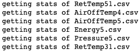
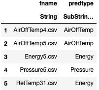
Figure 11 shows: a) a snapshot of the output during training and testing which extracts the statistical features of the time series; and b) the testing performance of the classifier. The training and testing data are labeled based on their sensor type for easier validation. The labels are not used as input during training. The classification workflow is purely driven by the statistical features. The prediction indicates 80% accuracy.

……….

……….

Figure 11: Extraction of Statistical Features for Training and Prediction. By convention, the TSClassifier validates the ground truth based on the filename which contains the label of the sensor type disregarding the numerical component.

4 Extending TSML with Scikit-Learn and Caret

In the latest TSML version (2.3.4 and above), we refactored the base TSML to only include pure Julia code implementations and moved the external libs and binary dependencies into the TSMLextra package. One major reason is to have a smaller code base so that it can be easily maintained and rapidly deployed in a dockerized solution for Kubernetes or IBM’s OpenShift cluster. Moreover, smaller codes make static compilation fast for smaller docker image in cloud deployment.

There are cases where the main task of time series classification requires more complex ensemble model using hierarchy or tree structure where members are composed of heterogeneous ML learners derived from binaries in different languages. For illustration purposes, we will show how to ensemble ML libraries from Scikit-Learn and Caret using TSML meta-ensembles that support the fit! and transform! APIs.

4.1 Parallel TSML Using Distributed Workflow

We will use Julia’s built-in support for parallelism by using the Distributed standard library. We also let Julia detect the number of processors available and activate them using the following statements:

[language = Julia] using Distributed nprocs() == 1 & addprocs()

With several workers active, we use the @everywhere macro to load the necessary filters and transformers to all workers.

[language = Julia] @everywhere using TSML @everywhere using TSMLextra @everywhere using DataFrames @everywhere using Random @everywhere using Statistics @everywhere using StatsBase: iqr @everywhere using RDatasets

With all the necessary TSML functions loaded, we can now setup the different MLs starting with some learners from Caret and Scikit-Learn. The list is not exhaustive for demonstration purposes.

[language = Julia] # Caret ML @everywhere caret_svmlinear = CaretLearner(Dict(:learner=>"svmLinear")) @everywhere caret_treebag = CaretLearner(Dict(:learner=>"treebag"))

# Scikit-Learn ML @everywhere sk_knn = SKLearner(Dict(:learner=>"KNeighborsClassifier")) @everywhere sk_gb = SKLearner(Dict(:learner=> "GradientBoostingClassifier", :impl_args=>Dict(:n_estimators=>10))) @everywhere sk_extratree = SKLearner(Dict(:learner=>"ExtraTreesClassifier", :impl_args=>Dict(:n_estimators=>10))) @everywhere sk_rf = SKLearner(Dict(:learner=> "RandomForestClassifier", :impl_args=>Dict(:n_estimators=>10)))

Let us setup ML instances from a pure Julia implementation of learners and ensembles wrapped from the DecisionTree.jl package [decisiontree2008, orchestra2014, combineml2016, tsmlextra2019].

[language = Julia] # Julia ML @everywhere jrf = RandomForest() @everywhere jpt = PrunedTree() @everywhere jada = Adaboost()

# Julia Ensembles @everywhere jvote_ens=VoteEnsemble(Dict( :learners=>[jrf,jpt,sk_gb,sk_extratree,sk_rf])) @everywhere jstack_ens=StackEnsemble(Dict( :learners=>[jrf,jpt,sk_gb,sk_extratree,sk_rf])) @everywhere jbest_ens=BestLearner(Dict( :learners=>[jrf,sk_gb,sk_rf])) @everywhere jsuper_ens=VoteEnsemble(Dict( :learners=>[jvote_ens,jstack_ens, jbest_ens,sk_rf,sk_gb]))

Next, we setup the pipeline for training and prediction.

[language = Julia] @everywhere function predict(learner, data,train_ind,test_ind) features = convert(Matrix,data[:, 1:(end-1)]) labels = convert(Array,data[:, end]) # Create pipeline pipeline = Pipeline( Dict( :transformers => [ OneHotEncoder(), # nominal to bits Imputer(), # Imputes NA values StandardScaler(), # normalize learner # Predicts labels on instances ] ) ) # Train fit!(pipeline, features[train_ind, :], labels[train_ind]) # Predict predictions = transform!(pipeline, features[test_ind, :]) # Assess predictions result = score(:accuracy, labels[test_ind], predictions) return result end

Finally, we setup the parallelmodel function to run different learners distributed to different workers running in parallel relying on Julia’s native support of parallelism. Take note that there are two parallelisms in the code. The first one is the distribution of task in different trials and the second one is the distribution of tasks among different models for each trial. It is interesting to note that with this relative compact function definition, the Julia language makes it easy to define a parallel task within another parallel task in a straightforward manner without any problem.

[language = Julia] function parallelmodel(learners::Dict, data::DataFrame;trials=5) models=collect(keys(learners)) ctable=@distributed (vcat) for i=1:trials # Split into training and test sets Random.seed!(3i) (trndx, tstndx) = holdout(size(data, 1), 0.20) acc=@distributed (vcat) for model in models res=predict(learners[model], data,trndx,tstndx) println("trial ",i,", ",model," => ", round(res)) [model res i] end acc end df = ctable |> DataFrame rename!(df,:x1=>:model,:x2=>:acc,:x3=>:trial) gp=by(df,:model) do x DataFrame(mean=mean(x.acc),std=std(x.acc), n=length(x.acc)) end sort!(gp,:mean,rev=true) return gp end

We benchmark the performance of the different machine learners by creating a dictionary of workers containing instances of learners from Caret, Scikit-Learn, and Julia libraries. We pass the dictionary of learners to the parallelmodel function for evaluation.

[language = Julia] learners=Dict( :jvote_ens=>jvote_ens,:jstack_ens=>jstack_ens, :jbest_ens=>jbest_ens,:jrf=>jrf,:jada=>jada, :jsuper_ens=>jsuper_ens, :crt_svmlinear=>caret_svmlinear, :crt_treebag=>caret_treebag, :skl_knn=>sk_knn,:skl_gb=>sk_gb, :skl_extratree=>sk_extratree, :sk_rf=>sk_rf )

datadir = joinpath("tsdata/") tsdata = extract_features_from_timeseries(datadir) first(tsdata,5)

respar = parallelmodel(learners,tsdata;trials=3)

Figure 12: Output During Training with Several Workers

Figure 13: @distributed: Classification Performance in 3 Trials

The data used in the experiment are sample snapshots of the data in our building operations. For reproducibility, the data can be found in the juliacon2019-paper branch of TSML in Github: /data/benchmark/tsclassifier. There are four time series types, namely: AirOffTemp, Energy, Pressure, and RetTemp. We took a minimal number of samples and classes for the sake of discussion and demonstration purposes in this paper.

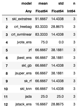
Figures 12 and 13 show a snapshot of running workers exploiting the distributed library of Julia and the classification performance of each model, respectively. There are 8 workers running in parallel over 12 different machine learning classifiers.

From the results, ExtraTree from Scikit-Learn has the best performance with 91.67% accuracy followed by TreeBag and SVMLinear from Caret library with 83.33 % accuracy for both. With this workflow, it becomes trivial to search for optimal model by running them in parallel relying on Julia to do the low-level tasks of scheduling and queueing as well as making sure that the dynamically available compute resources such as cpu cores and memory resources are fairly optimised.

4.2 Parallel TSML Using Threads Workflow

With Julia 1.3, lightweight multi-threading support in Julia becomes possible. We will be using the pure Julia-written ML models because installing external dependencies such as Caret MLs through RCall package has some issues with the alpha version of Julia 1.3 at this point in time. We will update this documentation and add more MLs once the issues are resolved.

The main difference in the workflow between Julia’s distributed computation model compared to the threaded model is the presence of @everywhere macro in the former for each function defined to indicate that these function definitions shall be exported to all running workers. Since threaded processes share the same memory model with the Julia main process, there is no need for this macro. Instead, threading workflow requires the use of ReentrantLock in the update of the global dataframe that accumulates the prediction performance of models running in their respective threads. In similar observation with the distributed framework, the threadedmodel function contains two parallelism: threads in different trials and threads among models in each trial. The function is surprisingly compact to implement threads within threads without issues and the main bottleneck happens only during the update operation of the global ctable dataframe.

[language = Julia] function threadedmodel(learners::Dict, data::DataFrame;trials=5) Random.seed!(3) models=collect(keys(learners)) global ctable = DataFrame() @threads for i=1:trials # Split into training and test sets (train_ind, test_ind) = holdout(size(data, 1), 0.20) mtx = SpinLock() @threads for themodel in models res=predict(learners[themodel], data,train_ind,test_ind) println(themodel," => ",round(res),", thread=",threadid()) lock(mtx) global ctable=vcat(ctable, DataFrame(model=themodel, acc=res)) unlock(mtx) end end df = ctable |> DataFrame gp=by(df,:model) do x DataFrame(mean=mean(x.acc), std=std(x.acc),n=nrow(x)) end sort!(gp,:mean,rev=true) return gp end

Let us define a set of learners that are written in pure Julia for this thread experiment.

[language = Julia] # Julia ML jrf = RandomForest(Dict(:impl_args=> Dict(:num_trees=>500))) jpt = PrunedTree() jada = Adaboost(Dict(:impl_args=> Dict(:num_iterations=>20)))

## Julia Ensembles jvote_ens=VoteEnsemble(Dict(:learners=> [jrf,jpt,jada])) jstack_ens=StackEnsemble(Dict(:learners=> [jrf,jpt,jada])) jbest_ens=BestLearner(Dict(:learners=> [jrf,jpt,jada])) jsuper_ens=VoteEnsemble(Dict(:learners=> [jvote_ens,jstack_ens,jbest_ens]));

Let us run in parallel the different models using the same dataset with that of the distributed workflow.

[language = Julia] using Base.Threads

learners=Dict( :jvote_ens=>jvote_ens, :jstack_ens=>jstack_ens, :jbest_ens=>jbest_ens, :jrf => jrf,:jada=>jada, :jsuper_ens=>jsuper