A Nonlinear Moment Model for Radiative Transfer Equation

Ruo Li,   Peng Song  and  Lingchao Zheng CAPT, LMAM & School of Mathematical Sciences, Peking University, Beijing, China, email: rli@math.pku.edu.cnInstitute of Applied Physics and Computational Mathematics, Beijing, China, email: song_peng@iapcm.ac.cnSchool of Mathematical Sciences, Peking University, Beijing, China, email: lczheng@pku.edu.cn
Abstract

We derive a nonlinear moment model for radiative transfer equation in 3D space, using the method to derive the nonlinear moment model for the radiative transfer equation in slab geometry. The resulted 3D HMPN𝐻𝑀subscript𝑃𝑁{H\!M\!P}_{\!N} model enjoys a list of mathematical advantages, including global hyperbolicity, rotational invariance, physical wave speeds, spectral accuracy, and correct higher-order Eddington approximation. Simulation examples are presented to validate the new model numerically.

Keywords: Radiative transfer equation; moment method; nonlinear model; global hyperbolicity.

1 Introduction

The radiative transfer equation (RTE) depicts the motion of photons and their interaction with the background medium. It has lots of applications, such as radiation astronomy [35], optical imaging [26, 40], neutron transport in reactor physics [37, 16], light transport in atmospheric radiative transfer [31] and heat transfer [27]. Due to the integro-differential form and the high-dimensionality of RTE, how to develop efficient methods to solve it numerically is an important but challenging topic. So far, the commonly used numerical methods can be categorized into two groups: the probabilistic methods, like the direct simulation Monte Carlo (DSMC) method [21, 3, 24, 14, 1], and the deterministic methods [4, 28, 39, 25, 13, 15, 36, 2, 17, 20, 19], such as the discrete ordinates method (SNsubscript𝑆𝑁S_{N}) [4, 28, 39], the moment methods [25, 13, 15, 2, 20, 19] and etc.

The discrete ordinates method (SNsubscript𝑆𝑁S_{N}) is one of the most popular numerical methods to simulate the RTE, which solve the RTE along with a discrete set of angular directions from a given quadrature set. However, the SNsubscript𝑆𝑁S_{N} model assumes that the particles can only move along the directions in the quadrature set, thus once the coordinate system is rotated, the results of the SNsubscript𝑆𝑁S_{N} model can be different. The lack of rotational invariance results in numerical artifacts, known as ray effects [28].

In order to reduce the complexity of the RTE, the moment method focuses on the evolution of a finite number of moments of the specific intensity, which avoids the high-dimensionality of directly solving the RTE. Since the governing equation of a lower order moment commonly contains higher order moments, the moment system is often not automatically closed. Hence one has to take a moment closure to close the moment system. A practical method for the moment closure is to construct an ansatz to approximate the specific intensity. The pioneer works in moment method include the spherical harmonics method (PNsubscript𝑃𝑁P_{N}) [37] and the maximum entropy method (MNsubscript𝑀𝑁M_{N}) [29, 15, 36]. The PNsubscript𝑃𝑁P_{N} model constructs the ansatz using spherical harmonic polynomials. It can be regarded as a polynomial expansion of the specific intensity around the equilibrium, which is a constant function. One of the flaws is that the resulting system may lead to nonphysical oscillations, or even worse, negative particle concentration [6, 7, 34]. The MNsubscript𝑀𝑁M_{N} model constructs the ansatz using the principle of maximum entropy, as the maximum entropy closure for Boltzmann equation [29, 15]. Unfortunately, no explicit expression of the moment closure for MNsubscript𝑀𝑁M_{N} model can be given when the order N2𝑁2N\geq 2. To implement the model numerically, one has to solve an ill-conditioned optimization problem to obtain an approximate moment closure. This almost prohibits the application of the MNsubscript𝑀𝑁M_{N} model.

Recently, a nonlinear moment model (called the MPN𝑀subscript𝑃𝑁{M\!P}_{\!N} model) was proposed in [20] for the RTE in slab geometry. This model takes the ansatz of the M1subscript𝑀1M_{1} model (the first order MNsubscript𝑀𝑁M_{N} model) as the weight function, then constructs the ansatz by expanding the specific intensity around the weight function in terms of orthogonal polynomials in the velocity variables. Numerical examples in [20] demonstrated a quite promising performance as an improved approximation of the intensity in comparison of the PNsubscript𝑃𝑁P_{N} model. The MPN𝑀subscript𝑃𝑁{M\!P}_{\!N} model was further improved in [19] by a globally hyperbolic regularization following the framework developed in [8, 9, 10, 18]. We note that the regularization in [19] is a subtle modification of the work in [10] instead of a direct application. Otherwise, the resulting system may change the M1subscript𝑀1M_{1} model, which leads to a wrong higher-order Eddington approximation. Eventually, the HMPN𝐻𝑀subscript𝑃𝑁{H\!M\!P}_{\!N} model was proposed in [19] with not only global hyperbolicity, but also a physical higher-order Eddington approximation.

Encouraged by the elegant mathematical structure and the promising numerical performance of the HMPN𝐻𝑀subscript𝑃𝑁{H\!M\!P}_{\!N} model for RTE in slab geometry, we in this paper try to extend the method to derive the HMPN𝐻𝑀subscript𝑃𝑁{H\!M\!P}_{\!N} model for 3D problems. The steps of the extension are clear while there are still numerous difficulties. Fortunately, the 3D M1subscript𝑀1M_{1} model is explicit, which allow us to construct the ansatz to approximate the specific intensity using again the weighted polynomials with the weight function is the ansatz of the M1subscript𝑀1M_{1} model. To construct the function space of the weighted polynomials, we need to give the orthogonal polynomial basis with respect to the weight function. For the slab geometry [20], this can be implemented by a simple Gram-Schmidt orthogonalization. For the 3D case, we have to use quasi-orthogonal polynomials rather than orthogonal polynomials. Otherwise, it can be extremely involving to accomplish the calculation, which makes further analysis to the resulted model prohibited. We propose a procedure to make a quasi Gram-Schmidt orthogonalization to obtain the quasi-orthogonal polynomials in explicit expressions. This provides us a 3D MPN𝑀subscript𝑃𝑁{M\!P}_{\!N} model in explicit formation, which can be mathematically analyzed. To achieve global hyperbolicity, we still adopt the method in [19] to regularize the 3D MPN𝑀subscript𝑃𝑁{M\!P}_{\!N} model. Quite smoothly a globally hyperbolic 3D HMPN𝐻𝑀subscript𝑃𝑁{H\!M\!P}_{\!N} model is eventually attained with a list of fabulous mathematical natures inherited from its 1D counterpart for the slab geometry. The resulted model is rotational invariant, with wave speeds not greater than that of light, spectral approximation accuracy, and correct higher-order Eddington approximation. We carry out preliminary numerical simulating using an abruptly splitting scheme to validate the new 3D HMPN𝐻𝑀subscript𝑃𝑁{H\!M\!P}_{\!N} model. Some numerical examples on typical problems are presented with satisfactory performance.

The rest of this paper is arranged as follows. In Section 2, we briefly introduce the moment methods for RTE, and review how the MPN𝑀subscript𝑃𝑁{M\!P}_{\!N} and the HMPN𝐻𝑀subscript𝑃𝑁{H\!M\!P}_{\!N} model in slab geometry were derived in [20, 19]. In Section 3, we derive the 3D MPN𝑀subscript𝑃𝑁{M\!P}_{\!N} model and prove that the model is rotational invariant. The hyperbolic regularization is applied to give the HMPN𝐻𝑀subscript𝑃𝑁{H\!M\!P}_{\!N} model in Section 4. The model is analyzed in detail therein. In Section 5, we introduce the numerical scheme to carry out numerical simulations and present some numerical examples. The paper is then ended with a short conclusion remarks.

2 Preliminary

To model radiative transfer, the governing equation is a time-dependent equation of the specific intensity I𝐼I as

1cIt+𝛀𝒙I=𝒮(I),1𝑐𝐼𝑡𝛀subscript𝒙𝐼𝒮𝐼\frac{1}{c}\dfrac{\partial{I}}{\partial{t}}+\bm{\Omega}\cdot\nabla_{\bm{x}}I={\mathcal{S}}(I), (2.1)

where c𝑐c is the speed of light, and the specific intensity I=I(t,𝒙;𝛀,ν)𝐼𝐼𝑡𝒙𝛀𝜈I=I(t,\bm{x};\bm{\Omega},\nu) depends on time t+𝑡superscriptt\in\mathbb{R}^{+}, the spatial coordinate of the photon 𝒙3𝒙superscript3\bm{x}\in\mathbb{R}^{3}, the velocity direction 𝛀𝕊2𝛀superscript𝕊2\bm{\Omega}\in\mathbb{S}^{2} and the frequency ν+𝜈superscript\nu\in\mathbb{R}^{+}. In this paper, our study omits the independent variable ν𝜈\nu that I𝐼I is a function of t𝑡t, 𝒙𝒙\bm{x} and 𝛀𝛀\bm{\Omega} only. The right hand side 𝒮(I)𝒮𝐼{\mathcal{S}}(I) denotes the actions by the background medium on the photons. A form of 𝒮(I)𝒮𝐼{\mathcal{S}}(I) adopted commonly was given in [5, 33] as

𝒮(I)=σtI+14πacσaT4+14πσs𝕊2Id𝛀+s4π,𝒮𝐼subscript𝜎𝑡𝐼14𝜋𝑎𝑐subscript𝜎𝑎superscript𝑇414𝜋subscript𝜎𝑠subscriptsuperscript𝕊2𝐼differential-d𝛀𝑠4𝜋{\mathcal{S}}(I)=-\sigma_{t}I+\frac{1}{4\pi}ac\sigma_{a}T^{4}+\frac{1}{4\pi}\sigma_{s}\int_{\mathbb{S}^{2}}I\,\mathrm{d}\bm{\Omega}+\frac{s}{4\pi}, (2.2)

where a𝑎a is the radiation constant, and s=s(t,𝒙)𝑠𝑠𝑡𝒙s=s(t,\bm{x}) is an isotropic external source of radiation. The scattering coefficient σssubscript𝜎𝑠\sigma_{s}, the absorption coefficient σasubscript𝜎𝑎\sigma_{a}, and the material temperature T(t,𝒙)𝑇𝑡𝒙T(t,\bm{x}) depend on time t𝑡t and the spatial position 𝒙𝒙\bm{x}. The total opacity coefficient is σt=σa+σssubscript𝜎𝑡subscript𝜎𝑎subscript𝜎𝑠\sigma_{t}=\sigma_{a}+\sigma_{s}.

In case that the problems slab geometry and spherical symmetric geometry are considered, the 3D RTE (2.1) can be simplified to 1D problem. Precisely, in the slab geometry, the specific intensity depends only upon the single spatial coordinate z𝑧z and the single angular coordinate arccosμ𝜇\arccos\mu, the angle between 𝛀𝛀\bm{\Omega} and the z𝑧z-axis. Then the specific intensity becomes I=I(z,μ)𝐼𝐼𝑧𝜇I=I(z,\mu), and (2.1) is simplified as

1cIt+μIz=𝒮(I).1𝑐𝐼𝑡𝜇𝐼𝑧𝒮𝐼\dfrac{1}{c}\dfrac{\partial{I}}{\partial{t}}+\mu\dfrac{\partial{I}}{\partial{z}}={\mathcal{S}}(I). (2.3)

The spherical geometry with perfect symmetry is a slightly more complicated case. The RTE, where the specific intensity depends upon only on the distance from the origin r=𝒙𝑟norm𝒙r=\|\bm{x}\|, and the angular variable arccosμ𝜇\arccos\mu, which is the angle between 𝛀𝛀\bm{\Omega} and 𝒙𝒙\bm{x}. In this case, I=I(r,μ)𝐼𝐼𝑟𝜇I=I(r,\mu), and the 3D RTE (2.1) is simplified as

1cIt+μIr+1μ2rIμ=𝒮(I).1𝑐𝐼𝑡𝜇𝐼𝑟1superscript𝜇2𝑟𝐼𝜇𝒮𝐼\dfrac{1}{c}\dfrac{\partial{I}}{\partial{t}}+\mu\dfrac{\partial{I}}{\partial{r}}+\dfrac{1-\mu^{2}}{r}\dfrac{\partial{I}}{\partial{\mu}}={\mathcal{S}}(I). (2.4)

In [2, 20, 19, 30], for slab geometry and spherical symmetric geometry, some nonlinear moment models had been derived with global hyperbolicity and promising performance in handling problems with fair extreme specific intensity functions. The major aim of this paper is to develop models for 3D problems with similar techniques.

At first, we define the moments of the 3D specific intensity. Let α3𝛼superscript3\alpha\in\mathbb{N}^{3} be a 3D multi-index, i.e. α=(α1,α2,α3)T𝛼superscriptsubscript𝛼1subscript𝛼2subscript𝛼3𝑇\alpha=(\alpha_{1},\alpha_{2},\alpha_{3})^{T}, α1,α2,α3subscript𝛼1subscript𝛼2subscript𝛼3\alpha_{1},\alpha_{2},\alpha_{3}\in\mathbb{N}. We define a function of t𝑡t, and 𝒙𝒙\bm{x}, denoted by Iα(t,𝒙)subscriptdelimited-⟨⟩𝐼𝛼𝑡𝒙{\langle I\rangle}_{\alpha}(t,\bm{x}), as

Iα(t,𝒙)𝕊2𝛀αI(t,𝒙;𝛀)d𝛀,α3,formulae-sequencesubscriptdelimited-⟨⟩𝐼𝛼𝑡𝒙subscriptsuperscript𝕊2superscript𝛀𝛼𝐼𝑡𝒙𝛀differential-d𝛀𝛼superscript3{\langle I\rangle}_{\alpha}(t,\bm{x})\triangleq\int_{\mathbb{S}^{2}}\bm{\Omega}^{\alpha}I(t,\bm{x};\bm{\Omega})\,\mathrm{d}\bm{\Omega},\quad\alpha\in\mathbb{N}^{3}, (2.5)

where 𝛀α=Ω1α1Ω2α2Ω3α3superscript𝛀𝛼superscriptsubscriptΩ1subscript𝛼1superscriptsubscriptΩ2subscript𝛼2superscriptsubscriptΩ3subscript𝛼3\bm{\Omega}^{\alpha}=\Omega_{1}^{\alpha_{1}}\Omega_{2}^{\alpha_{2}}\Omega_{3}^{\alpha_{3}}. We call that Iαsubscriptdelimited-⟨⟩𝐼𝛼{\langle I\rangle}_{\alpha} is the α𝛼\alpha-th moment of the specific intensity I𝐼I.

Notice that 𝛀𝕊2𝛀superscript𝕊2\bm{\Omega}\in\mathbb{S}^{2} implies 𝛀=1norm𝛀1\|\bm{\Omega}\|=1, thus one has

d=13Iα+2ed=Iα,α3,formulae-sequencesuperscriptsubscript𝑑13subscriptdelimited-⟨⟩𝐼𝛼2subscript𝑒𝑑subscriptdelimited-⟨⟩𝐼𝛼for-all𝛼superscript3\sum_{d=1}^{3}{\langle I\rangle}_{\alpha+2e_{d}}={\langle I\rangle}_{\alpha},\qquad\forall\alpha\in\mathbb{N}^{3},

where edsubscript𝑒𝑑e_{d} represents the multi-index whose d𝑑d-th index is 1, and the else two indexes are 0. Therefore, we only need to consider these moments Iαsubscriptdelimited-⟨⟩𝐼𝛼{\langle I\rangle}_{\alpha}, α𝛼\alpha\in{\mathcal{I}}, where {\mathcal{I}} is a set of multi-indexes, defined by

{α:α3,α31}.conditional-set𝛼formulae-sequence𝛼superscript3subscript𝛼31{\mathcal{I}}\triangleq\left\{\alpha:\alpha\in\mathbb{N}^{3},\alpha_{3}\leq 1\right\}. (2.6)

The order of the multi-index α𝛼\alpha is defined as |α|=d=13αd𝛼superscriptsubscript𝑑13subscript𝛼𝑑|\alpha|=\sum_{d=1}^{3}\alpha_{d}, and we denote that N{α:α,|α|N}subscript𝑁conditional-set𝛼formulae-sequence𝛼𝛼𝑁{\mathcal{I}}_{N}\triangleq\left\{\alpha:\alpha\in{\mathcal{I}},|\alpha|\leq N\right\}. It is clear that once {Iα:αN}conditional-setsubscriptdelimited-⟨⟩𝐼𝛼𝛼subscript𝑁\left\{{\langle I\rangle}_{\alpha}:\alpha\in{\mathcal{I}}_{N}\right\} is determined, one can obtain {Iα:α3,|α|N}conditional-setsubscriptdelimited-⟨⟩𝐼𝛼formulae-sequence𝛼superscript3𝛼𝑁\left\{{\langle I\rangle}_{\alpha}:\alpha\in\mathbb{N}^{3},|\alpha|\leq N\right\}. This allows us to discuss Iαsubscriptdelimited-⟨⟩𝐼𝛼{\langle I\rangle}_{\alpha} for α𝛼\alpha\in{\mathcal{I}} only to derive reduced models.

Multiplying (2.1) by 𝛀αsuperscript𝛀𝛼\bm{\Omega}^{\alpha}, and taking the integration with respect to 𝛀𝛀\bm{\Omega} over 𝕊2superscript𝕊2\mathbb{S}^{2}, one can have

1cIαt+d=13Iα+edxd=𝒮(I)α,α.formulae-sequence1𝑐subscriptdelimited-⟨⟩𝐼𝛼𝑡superscriptsubscript𝑑13subscriptdelimited-⟨⟩𝐼𝛼subscript𝑒𝑑subscript𝑥𝑑subscriptdelimited-⟨⟩𝒮𝐼𝛼𝛼\frac{1}{c}\dfrac{\partial{{\langle I\rangle}_{\alpha}}}{\partial{t}}+\sum_{d=1}^{3}\dfrac{\partial{{\langle I\rangle}_{\alpha+e_{d}}}}{\partial{x_{d}}}={\langle{\mathcal{S}}(I)\rangle}_{\alpha},\quad{\alpha}\in{\mathcal{I}}. (2.7)

In order to derive a moment model for (2.1), we first truncate the system by discarding all the governing equations of high order moments Iαsubscriptdelimited-⟨⟩𝐼𝛼{\langle I\rangle}_{\alpha}, where |α|>N𝛼𝑁|\alpha|>N, for a given integer N𝑁N\in\mathbb{N}. The truncated moment system is

1cIαt+d=13Iα+edxd=𝒮(I)α,αN.formulae-sequence1𝑐subscriptdelimited-⟨⟩𝐼𝛼𝑡superscriptsubscript𝑑13subscriptdelimited-⟨⟩𝐼𝛼subscript𝑒𝑑subscript𝑥𝑑subscriptdelimited-⟨⟩𝒮𝐼𝛼𝛼subscript𝑁\frac{1}{c}\dfrac{\partial{{\langle I\rangle}_{\alpha}}}{\partial{t}}+\sum_{d=1}^{3}\dfrac{\partial{{\langle I\rangle}_{\alpha+e_{d}}}}{\partial{x_{d}}}={\langle{\mathcal{S}}(I)\rangle}_{\alpha},\quad{\alpha}\in{\mathcal{I}}_{N}. (2.8)

However, the governing equations of Iαsubscriptdelimited-⟨⟩𝐼𝛼{\langle I\rangle}_{\alpha}, |α|=N𝛼𝑁|\alpha|=N, involve three N+1𝑁1N+1 order moments Iα+edsubscriptdelimited-⟨⟩𝐼𝛼subscript𝑒𝑑{\langle I\rangle}_{\alpha+e_{d}} for d=1,2,3𝑑123d=1,2,3, thus the truncated system (2.8) is not closed. Therefore, we need to determine all these moments, {Iα,αN+1}subscriptdelimited-⟨⟩𝐼𝛼𝛼subscript𝑁1\left\{{\langle I\rangle}_{\alpha},\alpha\in{\mathcal{I}}_{N+1}\right\} to make this truncated system (2.8) closed.

We divide the moments in {Iα,αN+1}subscriptdelimited-⟨⟩𝐼𝛼𝛼subscript𝑁1\left\{{\langle I\rangle}_{\alpha},\alpha\in{\mathcal{I}}_{N+1}\right\} into two parts: lower-order moments (also referred as known moments later on), and higher-order moments (also referred as unknown moments later on).

Iα,αN+1,|α|NIα,αN+1,|α|=N+1lower-order momentshigher-order moments(known moments)(unknown moments)formulae-sequencesubscriptdelimited-⟨⟩𝐼𝛼𝛼subscript𝑁1𝛼𝑁missing-subexpressionformulae-sequencesubscriptdelimited-⟨⟩𝐼𝛼𝛼subscript𝑁1𝛼𝑁1missing-subexpressionlower-order momentsmissing-subexpressionhigher-order moments(known moments)missing-subexpression(unknown moments)\begin{array}[H]{ccc}{\langle I\rangle}_{\alpha},\alpha\in{\mathcal{I}}_{N+1},|\alpha|\leq N&&{\langle I\rangle}_{\alpha},\alpha\in{\mathcal{I}}_{N+1},|\alpha|=N+1\\ \Downarrow&&\Downarrow\\ \text{lower-order moments}&&\text{higher-order moments}\\ \text{({\it known moments})}&&\text{({\it unknown moments})}\end{array} (2.9)

The aim of the so-called moment closure to this system is to approximate the unknown moments as functions of known moments, saying to give a formulation as

IαEα=Eα(Iβ,βN),for αN+1,|α|=N+1.formulae-sequencesubscriptdelimited-⟨⟩𝐼𝛼subscript𝐸𝛼subscript𝐸𝛼subscriptdelimited-⟨⟩𝐼𝛽𝛽subscript𝑁formulae-sequencefor 𝛼subscript𝑁1𝛼𝑁1{\langle I\rangle}_{\alpha}\approx E_{\alpha}=E_{\alpha}({\langle I\rangle}_{\beta},\beta\in{\mathcal{I}}_{N}),\quad\text{for }\alpha\in{\mathcal{I}}_{N+1},|\alpha|=N+1. (2.10)

To achieve this goal, a practical approach is to construct an ansatz for the specific intensity. Precisely, let Eαsubscript𝐸𝛼E_{\alpha}, αN𝛼subscript𝑁\alpha\in{\mathcal{I}}_{N}, be the known moments for a certain unknown specific intensity I𝐼I. Then one may propose an expression I^(𝛀;Eα,αN)^𝐼𝛀subscript𝐸𝛼𝛼subscript𝑁\hat{I}(\bm{\Omega};E_{\alpha},\alpha\in{\mathcal{I}}_{N}), called an ansatz to approximate I𝐼I, such that

I^(;Eα,αN)α=Eα,αN.formulae-sequencesubscriptdelimited-⟨⟩^𝐼subscript𝐸𝛼𝛼subscript𝑁𝛼subscript𝐸𝛼𝛼subscript𝑁{\langle\hat{I}(\cdot;E_{\alpha},\alpha\in{\mathcal{I}}_{N})\rangle}_{\alpha}=E_{\alpha},\quad\alpha\in{\mathcal{I}}_{N}. (2.11)

Often we require that I^^𝐼\hat{I} is uniquely determined by the consistency relations (2.11). With I^^𝐼\hat{I} given, the higher-order moments of I𝐼I are then approximated by the higher-order moments of I^^𝐼\hat{I}, i.e.,

Eα=I^(;Eβ,βN)α,αN+1,|α|=N+1.formulae-sequencesubscript𝐸𝛼subscriptdelimited-⟨⟩^𝐼subscript𝐸𝛽𝛽subscript𝑁𝛼formulae-sequence𝛼subscript𝑁1𝛼𝑁1E_{\alpha}={\langle\hat{I}(\cdot;E_{\beta},\beta\in{\mathcal{I}}_{N})\rangle}_{\alpha},\quad\alpha\in{\mathcal{I}}_{N+1},|\alpha|=N+1. (2.12)

Therefore, one may take the closed moment system

1cEαt+d=13Eα+edxd=𝒮(I^)α,αN,formulae-sequence1𝑐subscript𝐸𝛼𝑡superscriptsubscript𝑑13subscript𝐸𝛼subscript𝑒𝑑subscript𝑥𝑑subscriptdelimited-⟨⟩𝒮^𝐼𝛼𝛼subscript𝑁\frac{1}{c}\dfrac{\partial{E_{\alpha}}}{\partial{t}}+\sum_{d=1}^{3}\dfrac{\partial{E_{\alpha+e_{d}}}}{\partial{x_{d}}}=\langle{\mathcal{S}}(\hat{I})\rangle_{\alpha},\quad\alpha\in{\mathcal{I}}_{N}, (2.13)

as the reduced model to approximate the original RTE, where Eα+edsubscript𝐸𝛼subscript𝑒𝑑E_{\alpha+e_{d}} are functions of Eαsubscript𝐸𝛼E_{\alpha}, αN𝛼subscript𝑁\alpha\in{\mathcal{I}}_{N}, defined in (2.10) and (2.12).

Many existing models can be regarded as consequences using this moment closure approach. For example, the PNsubscript𝑃𝑁P_{N} model [25], the MNsubscript𝑀𝑁M_{N} model [29, 15], the positive PNsubscript𝑃𝑁P_{N} model [22], the B2subscript𝐵2B_{2} model [2], and the MPN𝑀subscript𝑃𝑁{M\!P}_{\!N} model [20] are in this fold. The MPN𝑀subscript𝑃𝑁{M\!P}_{\!N} model we proposed in [20], and then improved in [19] as the HMPN𝐻𝑀subscript𝑃𝑁{H\!M\!P}_{\!N} model, is limited for problems in slab geometry, where it exhibits satisfactory numerical performance for some standard benchmarks. To extend the method therein to 3D RTE, below we first briefly review the methods in [20, 19] to derive models in slab geometry to clarify our idea.

The MPN𝑀subscript𝑃𝑁{M\!P}_{\!N} model derived in [20] for RTE in slab geometry is based on a method to combine the PNsubscript𝑃𝑁P_{N} model and the MNsubscript𝑀𝑁M_{N} model, which was implemented by expanding the specific intensity around the ansatz of the M1subscript𝑀1M_{1} model in terms of orthogonal polynomials. The ansatz of the M1subscript𝑀1M_{1} model in slab geometry is

I^M1=ε(1+c0μ)4,subscript^𝐼subscript𝑀1𝜀superscript1subscript𝑐0𝜇4\hat{I}_{M_{1}}=\frac{\varepsilon}{(1+c_{0}\mu)^{4}}, (2.14)

where ε𝜀\varepsilon and c0subscript𝑐0c_{0} are determined by the 00-th moment E0subscript𝐸0E_{0} and 111-th moment E1subscript𝐸1E_{1}, formulated as

c0=3E1/E02+43(E1/E0)2,ε=3(1c02)32(3+c02).formulae-sequencesubscript𝑐03subscript𝐸1subscript𝐸0243superscriptsubscript𝐸1subscript𝐸02𝜀3superscript1superscriptsubscript𝑐02323superscriptsubscript𝑐02c_{0}=-\frac{3E_{1}/E_{0}}{2+\sqrt{4-3(E_{1}/E_{0})^{2}}},\quad\varepsilon=\frac{3(1-c_{0}^{2})^{3}}{2(3+c_{0}^{2})}. (2.15)

Then the specific intensity is approximated by a weighted polynomial, with the weight function

ω[c0](μ)=1(1+c0μ)4.superscript𝜔delimited-[]subscript𝑐0𝜇1superscript1subscript𝑐0𝜇4\omega^{[c_{0}]}(\mu)=\frac{1}{(1+c_{0}\mu)^{4}}. (2.16)

The function space of the weighted polynomials is

N[c0]{ω[c0]k=0Ngkμk}.subscriptsuperscriptdelimited-[]subscript𝑐0𝑁superscript𝜔delimited-[]subscript𝑐0superscriptsubscript𝑘0𝑁subscript𝑔𝑘superscript𝜇𝑘\mathbb{H}^{[c_{0}]}_{N}\triangleq\left\{\omega^{[c_{0}]}\sum_{k=0}^{N}g_{k}\mu^{k}\right\}. (2.17)

Then the ansatz of the MPN𝑀subscript𝑃𝑁{M\!P}_{\!N} model is written as

I^(μ;E0,,EN)i=0NfiΦi[c0](μ)N[c0],Φi[c0](μ)=ϕi[c0](μ)ω[c0](μ),formulae-sequence^𝐼𝜇subscript𝐸0subscript𝐸𝑁superscriptsubscript𝑖0𝑁subscript𝑓𝑖subscriptsuperscriptΦdelimited-[]subscript𝑐0𝑖𝜇subscriptsuperscriptdelimited-[]subscript𝑐0𝑁subscriptsuperscriptΦdelimited-[]subscript𝑐0𝑖𝜇subscriptsuperscriptitalic-ϕdelimited-[]subscript𝑐0𝑖𝜇superscript𝜔delimited-[]subscript𝑐0𝜇\hat{I}(\mu;E_{0},\cdots,E_{N})\triangleq\sum_{i=0}^{N}f_{i}\Phi^{[c_{0}]}_{i}(\mu)\in\mathbb{H}^{[c_{0}]}_{N},\quad\Phi^{[c_{0}]}_{i}(\mu)=\phi^{[c_{0}]}_{i}(\mu)\omega^{[c_{0}]}(\mu), (2.18)

where Φi[c0](μ)=ϕi[c0](μ)ω[c0](μ)subscriptsuperscriptΦdelimited-[]subscript𝑐0𝑖𝜇subscriptsuperscriptitalic-ϕdelimited-[]subscript𝑐0𝑖𝜇superscript𝜔delimited-[]subscript𝑐0𝜇\Phi^{[c_{0}]}_{i}(\mu)=\phi^{[c_{0}]}_{i}(\mu)\omega^{[c_{0}]}(\mu), i=0,1,,N𝑖01𝑁i=0,1,\cdots,N, are the basis functions, ϕi[c0](μ)subscriptsuperscriptitalic-ϕdelimited-[]subscript𝑐0𝑖𝜇\phi^{[c_{0}]}_{i}(\mu) are orthogonal polynomials with respect to the weight function, and fisubscript𝑓𝑖f_{i} are the expansion coefficients.

The orthogonal polynomials ϕk[c0](μ)subscriptsuperscriptitalic-ϕdelimited-[]subscript𝑐0𝑘𝜇\phi^{[c_{0}]}_{k}(\mu) can be calculated by a simple Gram-Schmidt orthogonalization, formulated as

ϕ0[c0](μ)=1,ϕj[c0](μ)=μjk=0j1𝒦j,k𝒦k,kϕk[c0](μ),j1,formulae-sequencesubscriptsuperscriptitalic-ϕdelimited-[]subscript𝑐00𝜇1formulae-sequencesubscriptsuperscriptitalic-ϕdelimited-[]subscript𝑐0𝑗𝜇superscript𝜇𝑗superscriptsubscript𝑘0𝑗1subscript𝒦𝑗𝑘subscript𝒦𝑘𝑘subscriptsuperscriptitalic-ϕdelimited-[]subscript𝑐0𝑘𝜇𝑗1\phi^{[c_{0}]}_{0}(\mu)=1,\quad\phi^{[c_{0}]}_{j}(\mu)=\mu^{j}-\sum_{k=0}^{j-1}\frac{{\mathcal{K}}_{j,k}}{{\mathcal{K}}_{k,k}}\phi^{[c_{0}]}_{k}(\mu),\quad j\geq 1, (2.19)

where 𝒦j,k=11μjϕk[c0](μ)ω[c0](μ)dμsubscript𝒦𝑗𝑘superscriptsubscript11superscript𝜇𝑗subscriptsuperscriptitalic-ϕdelimited-[]subscript𝑐0𝑘𝜇superscript𝜔delimited-[]subscript𝑐0𝜇differential-d𝜇{\mathcal{K}}_{j,k}=\int_{-1}^{1}\mu^{j}\phi^{[c_{0}]}_{k}(\mu)\omega^{[c_{0}]}(\mu)\,\mathrm{d}\mu, calculated by

𝒦0,0=ω[c0](μ)0,𝒦i,j=ω[c0](μ)i+jk=0j1𝒦j,k𝒦i,k𝒦k,k,1ji.formulae-sequencesubscript𝒦00subscriptdelimited-⟨⟩superscript𝜔delimited-[]subscript𝑐0𝜇0formulae-sequencesubscript𝒦𝑖𝑗subscriptdelimited-⟨⟩superscript𝜔delimited-[]subscript𝑐0𝜇𝑖𝑗superscriptsubscript𝑘0𝑗1subscript𝒦𝑗𝑘subscript𝒦𝑖𝑘subscript𝒦𝑘𝑘1𝑗𝑖{\mathcal{K}}_{0,0}={\langle\omega^{[c_{0}]}(\mu)\rangle}_{0},\quad{\mathcal{K}}_{i,j}={\langle\omega^{[c_{0}]}(\mu)\rangle}_{i+j}-\sum_{k=0}^{j-1}\frac{{\mathcal{K}}_{j,k}{\mathcal{K}}_{i,k}}{{\mathcal{K}}_{k,k}},\quad 1\leq j\leq i. (2.20)

Furthermore, by

f0=E0𝒦0,0,fi=1𝒦i,i(Eij=0i1𝒦i,jfj),1iN,formulae-sequencesubscript𝑓0subscript𝐸0subscript𝒦00formulae-sequencesubscript𝑓𝑖1subscript𝒦𝑖𝑖subscript𝐸𝑖superscriptsubscript𝑗0𝑖1subscript𝒦𝑖𝑗subscript𝑓𝑗1𝑖𝑁f_{0}=\dfrac{E_{0}}{{\mathcal{K}}_{0,0}},\quad f_{i}=\frac{1}{{\mathcal{K}}_{i,i}}\left(E_{i}-\sum_{j=0}^{i-1}{\mathcal{K}}_{i,j}f_{j}\right),\quad 1\leq i\leq N, (2.21)

one can determine the coefficients fksubscript𝑓𝑘f_{k}, and the ansatz I^(μ;E0,E1,EN)^𝐼𝜇subscript𝐸0subscript𝐸1subscript𝐸𝑁\hat{I}(\mu;E_{0},E_{1},\cdots E_{N}). Finally, we have the moment closure as

EN+1=k=0Nfk𝒦N+1,k.subscript𝐸𝑁1superscriptsubscript𝑘0𝑁subscript𝑓𝑘subscript𝒦𝑁1𝑘E_{N+1}=\sum_{k=0}^{N}f_{k}{\mathcal{K}}_{N+1,k}. (2.22)

Meanwhile, in the viewpoint of orthogonal projection, if we define the orthogonal projection to function space N[c0]subscriptsuperscriptdelimited-[]subscript𝑐0𝑁\mathbb{H}^{[c_{0}]}_{N},

𝒫N:f=k=0+fkΦk[c0](μ)𝒫Nf=k=0NfkΦk[c0](μ),:subscript𝒫𝑁𝑓superscriptsubscript𝑘0subscript𝑓𝑘subscriptsuperscriptΦdelimited-[]subscript𝑐0𝑘𝜇subscript𝒫𝑁𝑓superscriptsubscript𝑘0𝑁subscript𝑓𝑘subscriptsuperscriptΦdelimited-[]subscript𝑐0𝑘𝜇\mathcal{P}_{N}:f=\sum_{k=0}^{+\infty}f_{k}\Phi^{[c_{0}]}_{k}(\mu)\rightarrow\mathcal{P}_{N}f=\sum_{k=0}^{N}f_{k}\Phi^{[c_{0}]}_{k}(\mu), (2.23)

then the MPN𝑀subscript𝑃𝑁{M\!P}_{\!N} moment system can be written as

1c𝒫N𝒫NIt+𝒫Nμ𝒫NIz=𝒫N𝒮(𝒫NI).1𝑐subscript𝒫𝑁subscript𝒫𝑁𝐼𝑡subscript𝒫𝑁𝜇subscript𝒫𝑁𝐼𝑧subscript𝒫𝑁𝒮subscript𝒫𝑁𝐼\dfrac{1}{c}\mathcal{P}_{N}\dfrac{\partial{\mathcal{P}_{N}I}}{\partial{t}}+\mathcal{P}_{N}\mu\dfrac{\partial{\mathcal{P}_{N}I}}{\partial{z}}=\mathcal{P}_{N}{\mathcal{S}}(\mathcal{P}_{N}I). (2.24)

The weight function (2.16) permits the MPN𝑀subscript𝑃𝑁{M\!P}_{\!N} model to approximate a strongly anisotropic distribution with very high accuracy. In [19], the MPN𝑀subscript𝑃𝑁{M\!P}_{\!N} model was further improved by a hyperbolic regularization, which provides global hyperbolicity. To achieve the required hyperbolicity, the model reduction framework in [10, 18] suggests adding one more projection between the operators μ\mu\cdot and z\dfrac{\partial{\cdot}}{\partial{z}} in (2.24) to regularize the MPN𝑀subscript𝑃𝑁{M\!P}_{\!N} model to be globally hyperbolic, and the resulting model is

1c𝒫N𝒫NIt+𝒫Nμ𝒫N𝒫NIz=𝒫N𝒮(𝒫NI).1𝑐subscript𝒫𝑁subscript𝒫𝑁𝐼𝑡subscript𝒫𝑁𝜇subscript𝒫𝑁subscript𝒫𝑁𝐼𝑧subscript𝒫𝑁𝒮subscript𝒫𝑁𝐼\frac{1}{c}\mathcal{P}_{N}\dfrac{\partial{\mathcal{P}_{N}I}}{\partial{t}}+\mathcal{P}_{N}\mu\mathcal{P}_{N}\dfrac{\partial{\mathcal{P}_{N}I}}{\partial{z}}=\mathcal{P}_{N}{\mathcal{S}}(\mathcal{P}_{N}I). (2.25)

An interesting point observed in [19] is that this regularization changes the MPN𝑀subscript𝑃𝑁{M\!P}_{\!N} model when N=1𝑁1N=1. It is definitely inappropriate that the M1subscript𝑀1M_{1} model is changed by the regularization. In order to fix this defect, another weight function is introduced as

ω~[c0]=1(1+c0μ)5,superscript~𝜔delimited-[]subscript𝑐01superscript1subscript𝑐0𝜇5\tilde{\omega}^{[c_{0}]}=\frac{1}{(1+c_{0}\mu)^{5}}, (2.26)

and then a new function space is defined as

~N[c0]{ω~[c0]k=0Ngkμk}.subscriptsuperscript~delimited-[]subscript𝑐0𝑁superscript~𝜔delimited-[]subscript𝑐0superscriptsubscript𝑘0𝑁subscript𝑔𝑘superscript𝜇𝑘\tilde{\mathbb{H}}^{[c_{0}]}_{N}\triangleq\left\{\tilde{\omega}^{[c_{0}]}\sum_{k=0}^{N}g_{k}\mu^{k}\right\}. (2.27)

In this subspace, one can define the orthogonal polynomials ϕ~k[c0](μ)subscriptsuperscript~italic-ϕdelimited-[]subscript𝑐0𝑘𝜇\tilde{\phi}^{[c_{0}]}_{k}(\mu) and the basis function Φ~k[c0](μ)subscriptsuperscript~Φdelimited-[]subscript𝑐0𝑘𝜇\tilde{\Phi}^{[c_{0}]}_{k}(\mu), 0kN0𝑘𝑁0\leq k\leq N. Furthermore, a new projection 𝒫~Nsubscript~𝒫𝑁\tilde{\mathcal{P}}_{N} is defined as

𝒫~N:f=k=0+fkΦ~k[c0](μ)𝒫~Nf=k=0NfkΦ~k[c0](μ).:subscript~𝒫𝑁𝑓superscriptsubscript𝑘0subscript𝑓𝑘subscriptsuperscript~Φdelimited-[]subscript𝑐0𝑘𝜇subscript~𝒫𝑁𝑓superscriptsubscript𝑘0𝑁subscript𝑓𝑘subscriptsuperscript~Φdelimited-[]subscript𝑐0𝑘𝜇\tilde{\mathcal{P}}_{N}:f=\sum_{k=0}^{+\infty}f_{k}\tilde{\Phi}^{[c_{0}]}_{k}(\mu)\rightarrow\tilde{\mathcal{P}}_{N}f=\sum_{k=0}^{N}f_{k}\tilde{\Phi}^{[c_{0}]}_{k}(\mu). (2.28)

The new hyperbolic regularization in [19] adds one more projection 𝒫~Nsubscript~𝒫𝑁\tilde{\mathcal{P}}_{N} to give the HMPN𝐻𝑀subscript𝑃𝑁{H\!M\!P}_{\!N} model formulated as

1c𝒫~N𝒫NIt+𝒫~Nμ𝒫~N𝒫NIz=𝒫~N𝒮(𝒫NI).1𝑐subscript~𝒫𝑁subscript𝒫𝑁𝐼𝑡subscript~𝒫𝑁𝜇subscript~𝒫𝑁subscript𝒫𝑁𝐼𝑧subscript~𝒫𝑁𝒮subscript𝒫𝑁𝐼\frac{1}{c}\tilde{\mathcal{P}}_{N}\dfrac{\partial{\mathcal{P}_{N}I}}{\partial{t}}+\tilde{\mathcal{P}}_{N}\mu\tilde{\mathcal{P}}_{N}\dfrac{\partial{\mathcal{P}_{N}I}}{\partial{z}}=\tilde{\mathcal{P}}_{N}{\mathcal{S}}(\mathcal{P}_{N}I). (2.29)

It was revealed that the HMPN𝐻𝑀subscript𝑃𝑁{H\!M\!P}_{\!N} model enjoys some desired properties, such as

Property 1.
  1. 1.

    The HMPN𝐻𝑀subscript𝑃𝑁{H\!M\!P}_{\!N} model is globally hyperbolic.

  2. 2.

    The characteristic speeds of the HMPN𝐻𝑀subscript𝑃𝑁{H\!M\!P}_{\!N} model lie in [c,c]𝑐𝑐[-c,c].

  3. 3.

    The regularization vanishes for the case N=1𝑁1N=1.

  4. 4.

    Between the MPN𝑀subscript𝑃𝑁{M\!P}_{\!N} model and the HMPN𝐻𝑀subscript𝑃𝑁{H\!M\!P}_{\!N} model, the governing equation of Eksubscript𝐸𝑘E_{k}, k=0,,N1𝑘0𝑁1k=0,\dots,N-1 is not changed.

3 Moment Model Reduction

In this section, we adopt the strategy introduced in Section 2 to derive a MPN𝑀subscript𝑃𝑁{M\!P}_{\!N} type model for the 3D RTE at first.

3.1 Formal derivation

Let us start with the M1subscript𝑀1M_{1} model in 3D case. The ansatz of specific intensity is

I^M1(𝛀;E0,Ee1,Ee2,Ee3)=ε(1+𝒄0𝛀)4.subscript^𝐼subscript𝑀1𝛀subscript𝐸0subscript𝐸subscript𝑒1subscript𝐸subscript𝑒2subscript𝐸subscript𝑒3𝜀superscript1subscript𝒄0𝛀4\hat{I}_{M_{1}}(\bm{\Omega};E_{0},E_{e_{1}},E_{e_{2}},E_{e_{3}})=\dfrac{\varepsilon}{(1+\bm{c}_{0}\cdot\bm{\Omega})^{4}}. (3.1)

with the known moments E0subscript𝐸0E_{0}, Ee1subscript𝐸subscript𝑒1E_{e_{1}}, Ee2subscript𝐸subscript𝑒2E_{e_{2}}, and Ee3subscript𝐸subscript𝑒3E_{e_{3}}. We denote them as 𝑬0=(E0)Tsubscript𝑬0superscriptsubscript𝐸0𝑇\bm{E}_{0}=(E_{0})^{T}, and 𝑬1=(Ee1,Ee2,Ee3)Tsubscript𝑬1superscriptsubscript𝐸subscript𝑒1subscript𝐸subscript𝑒2subscript𝐸subscript𝑒3𝑇\bm{E}_{1}=(E_{e_{1}},E_{e_{2}},E_{e_{3}})^{T}, respectively. Direct calculation yields that

𝒄0=2+43(𝑬1/E0)2𝑬1/E0𝑬1𝑬1,subscript𝒄0243superscriptnormsubscript𝑬1subscript𝐸02normsubscript𝑬1subscript𝐸0subscript𝑬1normsubscript𝑬1\bm{c}_{0}=\dfrac{-2+\sqrt{4-3(\|\bm{E}_{1}\|/E_{0})^{2}}}{\|\bm{E}_{1}\|/E_{0}}\dfrac{\bm{E}_{1}}{\|\bm{E}_{1}\|}, (3.2)

Following [20], we approximate the specific intensity with a weighted polynomial, and the weight function is chosen as the ansatz of the M1subscript𝑀1M_{1} model, as (3.1). For simplicity, we take the weight function as

ω[𝒄0](𝛀)=1(1+𝒄0𝛀)4.superscript𝜔delimited-[]subscript𝒄0𝛀1superscript1subscript𝒄0𝛀4\omega^{[\bm{c}_{0}]}(\bm{\Omega})=\dfrac{1}{(1+\bm{c}_{0}\cdot\bm{\Omega})^{4}}.

Then the function space of weighted polynomials is defined as

N[𝒄0]{ω[𝒄0](𝛀)αNgα𝛀α}.subscriptsuperscriptdelimited-[]subscript𝒄0𝑁superscript𝜔delimited-[]subscript𝒄0𝛀subscript𝛼subscript𝑁subscript𝑔𝛼superscript𝛀𝛼\mathbb{H}^{[\bm{c}_{0}]}_{N}\triangleq\left\{\omega^{[\bm{c}_{0}]}(\bm{\Omega})\sum_{\alpha\in{\mathcal{I}}_{N}}g_{\alpha}\bm{\Omega}^{\alpha}\right\}. (3.3)

The ansatz of the 3D MPN𝑀subscript𝑃𝑁{M\!P}_{\!N} model I^(𝛀)^𝐼𝛀\hat{I}(\bm{\Omega}) is chosen to satisfy

I^N[𝒄0],I^α=Eα,αN.formulae-sequence^𝐼subscriptsuperscriptdelimited-[]subscript𝒄0𝑁formulae-sequencesubscriptdelimited-⟨⟩^𝐼𝛼subscript𝐸𝛼𝛼subscript𝑁\hat{I}\in\mathbb{H}^{[\bm{c}_{0}]}_{N},\quad\langle\hat{I}\rangle_{\alpha}=E_{\alpha},\quad\alpha\in{\mathcal{I}}_{N}.

In order to determine the ansatz I^^𝐼\hat{I}, we first rewrite I^^𝐼\hat{I} as

I^(t,𝒙;𝛀)=I^(t;𝑬)=αNfα(t,𝒙)ϕα[𝒄0](𝛀)ω[𝒄0(t,𝒙)](𝛀)N[𝒄0],^𝐼𝑡𝒙𝛀^𝐼𝑡𝑬subscript𝛼subscript𝑁subscript𝑓𝛼𝑡𝒙subscriptsuperscriptitalic-ϕdelimited-[]subscript𝒄0𝛼𝛀superscript𝜔delimited-[]subscript𝒄0𝑡𝒙𝛀subscriptsuperscriptdelimited-[]subscript𝒄0𝑁\hat{I}(t,\bm{x};\bm{\Omega})=\hat{I}(t;\bm{E})=\sum_{\alpha\in{\mathcal{I}}_{N}}f_{\alpha}(t,\bm{x})\phi^{[\bm{c}_{0}]}_{\alpha}(\bm{\Omega})\omega^{[\bm{c}_{0}(t,\bm{x})]}(\bm{\Omega})\in\mathbb{H}^{[\bm{c}_{0}]}_{N}, (3.4)

where ϕα[𝒄0],αNsubscriptsuperscriptitalic-ϕdelimited-[]subscript𝒄0𝛼𝛼subscript𝑁\phi^{[\bm{c}_{0}]}_{\alpha},\alpha\in{\mathcal{I}}_{N} are quasi-orthogonal polynomials with respect to the weight function ω[𝒄0]superscript𝜔delimited-[]subscript𝒄0\omega^{[\bm{c}_{0}]}, and fαsubscript𝑓𝛼f_{\alpha} are the corresponding coefficients. On the quasi-orthogonal polynomials, we define the inner product

f,gN[𝒄0]𝕊2fgω[𝒄0]d𝛀,subscript𝑓𝑔subscriptsuperscriptdelimited-[]subscript𝒄0𝑁subscriptsuperscript𝕊2𝑓𝑔superscript𝜔delimited-[]subscript𝒄0differential-d𝛀\left\langle{f},{g}\right\rangle_{\mathbb{H}^{[\bm{c}_{0}]}_{N}}\triangleq\int_{\mathbb{S}^{2}}fg\omega^{[\bm{c}_{0}]}\,\mathrm{d}\bm{\Omega}, (3.5)

then the quasi-orthogonal polynomials ϕα[𝒄0]subscriptsuperscriptitalic-ϕdelimited-[]subscript𝒄0𝛼\phi^{[\bm{c}_{0}]}_{\alpha} satisfy that

ϕα[𝒄0],ϕβ[𝒄0]N[𝒄0]=𝕊2ϕα[𝒄0](𝛀)ϕβ[𝒄0](𝛀)ω[𝒄0](𝛀)d𝛀=0,when |α||β|.formulae-sequencesubscriptsubscriptsuperscriptitalic-ϕdelimited-[]subscript𝒄0𝛼subscriptsuperscriptitalic-ϕdelimited-[]subscript𝒄0𝛽subscriptsuperscriptdelimited-[]subscript𝒄0𝑁subscriptsuperscript𝕊2subscriptsuperscriptitalic-ϕdelimited-[]subscript𝒄0𝛼𝛀subscriptsuperscriptitalic-ϕdelimited-[]subscript𝒄0𝛽𝛀superscript𝜔delimited-[]subscript𝒄0𝛀differential-d𝛀0when 𝛼𝛽\left\langle{\phi^{[\bm{c}_{0}]}_{\alpha}},{\phi^{[\bm{c}_{0}]}_{\beta}}\right\rangle_{\mathbb{H}^{[\bm{c}_{0}]}_{N}}=\int_{\mathbb{S}^{2}}\phi^{[\bm{c}_{0}]}_{\alpha}(\bm{\Omega})\phi^{[\bm{c}_{0}]}_{\beta}(\bm{\Omega})\omega^{[\bm{c}_{0}]}(\bm{\Omega})\,\mathrm{d}\bm{\Omega}=0,\quad\text{when }|\alpha|\neq|\beta|. (3.6)

Moreover, the quasi-polynomial ϕα[𝒄0]subscriptsuperscriptitalic-ϕdelimited-[]subscript𝒄0𝛼\phi^{[\bm{c}_{0}]}_{\alpha} satisfies that its only |α|𝛼|\alpha|-order term is 𝛀αsuperscript𝛀𝛼\bm{\Omega}^{\alpha}, i.e.

ϕα[𝒄0]=𝛀α+β|α|1hα,β𝛀β.subscriptsuperscriptitalic-ϕdelimited-[]subscript𝒄0𝛼superscript𝛀𝛼subscript𝛽subscript𝛼1subscript𝛼𝛽superscript𝛀𝛽\phi^{[\bm{c}_{0}]}_{\alpha}=\bm{\Omega}^{\alpha}+\sum_{\beta\in{\mathcal{I}}_{|\alpha|-1}}h_{\alpha,\beta}\bm{\Omega}^{\beta}. (3.7)

For later usage, we denote the quasi-orthogonal functions

Φα[𝒄0]=ϕα[𝒄0]ω[𝒄0].subscriptsuperscriptΦdelimited-[]subscript𝒄0𝛼subscriptsuperscriptitalic-ϕdelimited-[]subscript𝒄0𝛼superscript𝜔delimited-[]subscript𝒄0\Phi^{[\bm{c}_{0}]}_{\alpha}=\phi^{[\bm{c}_{0}]}_{\alpha}\omega^{[\bm{c}_{0}]}. (3.8)
Remark 1.

Let us remark that ϕα[𝐜0]subscriptsuperscriptitalic-ϕdelimited-[]subscript𝐜0𝛼\phi^{[\bm{c}_{0}]}_{\alpha}, α𝛼\alpha\in{\mathcal{I}} are quasi-orthogonal polynomials, rather than orthogonal polynomials. In other words, ϕα[𝐜0],ϕβ[𝐜0]N[𝐜0]subscriptsubscriptsuperscriptitalic-ϕdelimited-[]subscript𝐜0𝛼subscriptsuperscriptitalic-ϕdelimited-[]subscript𝐜0𝛽subscriptsuperscriptdelimited-[]subscript𝐜0𝑁\left\langle{\phi^{[\bm{c}_{0}]}_{\alpha}},{\phi^{[\bm{c}_{0}]}_{\beta}}\right\rangle_{\mathbb{H}^{[\bm{c}_{0}]}_{N}} can be non-zero for |α|=|β|𝛼𝛽|\alpha|=|\beta| and αβ𝛼𝛽\alpha\neq\beta.

Let us construct these quasi-orthogonal polynomials ϕα[𝒄0]subscriptsuperscriptitalic-ϕdelimited-[]subscript𝒄0𝛼\phi^{[\bm{c}_{0}]}_{\alpha} by the Gram-Schmidt orthogonalization. This Gram-Schmidt orthogonalization is different from the 1D case used in [20]. We denote αsubscript𝛼{\mathcal{E}}_{\alpha} as the moments of the weight function αω[𝒄0]αsubscript𝛼subscriptdelimited-⟨⟩superscript𝜔delimited-[]subscript𝒄0𝛼{\mathcal{E}}_{\alpha}\triangleq\langle\omega^{[\bm{c}_{0}]}\rangle_{\alpha} for later usage.

In (3.2), we denote 𝑬0subscript𝑬0\bm{E}_{0} and 𝑬1subscript𝑬1\bm{E}_{1} as the vector of moments of order 00 and order 111. In the following discussion, we will continue to use this notation, i.e. we denote 𝑬ksubscript𝑬𝑘\bm{E}_{k} as the vector of moments of order k𝑘k, whose dimension is 2k+12𝑘12k+1. Similarly, we can denote ϕ[𝒄𝟎]ksubscriptsuperscriptbold-italic-ϕdelimited-[]subscript𝒄0𝑘\bm{\phi^{[\bm{c}_{0}]}}_{k}, 𝚽[𝒄𝟎]ksubscriptsuperscript𝚽delimited-[]subscript𝒄0𝑘\bm{\Phi^{[\bm{c}_{0}]}}_{k}, 𝒇ksubscript𝒇𝑘\bm{f}_{k} and 𝓔ksubscript𝓔𝑘\bm{{\mathcal{E}}}_{k}. Using this notation, the moment closure

Eα(Eβ,βN),|α|=N+1,αformulae-sequencesubscript𝐸𝛼subscript𝐸𝛽𝛽subscript𝑁𝛼𝑁1𝛼E_{\alpha}(E_{\beta},\beta\in{\mathcal{I}}_{N}),\quad|\alpha|=N+1,\alpha\in{\mathcal{I}}

can be rewritten as

𝑬N+1(𝑬k, 0kN).subscript𝑬𝑁1subscript𝑬𝑘 0𝑘𝑁\bm{E}_{N+1}(\bm{E}_{k},\ 0\leq k\leq N).

We denote by 𝝋ksubscript𝝋𝑘\bm{\varphi}_{k} to be the vector of 𝛀αsuperscript𝛀𝛼\bm{\Omega}^{\alpha}, α𝛼\alpha\in{\mathcal{I}} and |α|=k𝛼𝑘|\alpha|=k. Using these notations, the ansatz (3.4) is rewritten as

I^=k=0N𝒇k𝚽[𝒄𝟎]k=ω[𝒄0]k=0N𝒇kϕ[𝒄𝟎]k.^𝐼superscriptsubscript𝑘0𝑁subscript𝒇𝑘subscriptsuperscript𝚽delimited-[]subscript𝒄0𝑘superscript𝜔delimited-[]subscript𝒄0superscriptsubscript𝑘0𝑁subscript𝒇𝑘subscriptsuperscriptbold-italic-ϕdelimited-[]subscript𝒄0𝑘\hat{I}=\sum_{k=0}^{N}\bm{f}_{k}\bm{\Phi^{[\bm{c}_{0}]}}_{k}=\omega^{[\bm{c}_{0}]}\sum_{k=0}^{N}\bm{f}_{k}\bm{\phi^{[\bm{c}_{0}]}}_{k}. (3.9)

We denote the inner product as

𝒦α,β𝛀α,ϕβ[𝒄0]N[𝒄0],subscript𝒦𝛼𝛽subscriptsuperscript𝛀𝛼subscriptsuperscriptitalic-ϕdelimited-[]subscript𝒄0𝛽subscriptsuperscriptdelimited-[]subscript𝒄0𝑁{\mathcal{K}}_{\alpha,\beta}\triangleq\left\langle{\bm{\Omega}^{\alpha}},{\phi^{[\bm{c}_{0}]}_{\beta}}\right\rangle_{\mathbb{H}^{[\bm{c}_{0}]}_{N}},

according to the properties of the quasi-orthogonal polynomials ϕα[𝒄0]subscriptsuperscriptitalic-ϕdelimited-[]subscript𝒄0𝛼\phi^{[\bm{c}_{0}]}_{\alpha} (3.6) and (3.7), we have

𝒦α,β=0, when |α|<|β|;𝒦α,β=ϕα[𝒄0],ϕβ[𝒄0]N[𝒄0]=𝒦β,α, when |α|=|β|.formulae-sequenceformulae-sequencesubscript𝒦𝛼𝛽0formulae-sequence when 𝛼𝛽subscript𝒦𝛼𝛽subscriptsubscriptsuperscriptitalic-ϕdelimited-[]subscript𝒄0𝛼subscriptsuperscriptitalic-ϕdelimited-[]subscript𝒄0𝛽subscriptsuperscriptdelimited-[]subscript𝒄0𝑁subscript𝒦𝛽𝛼 when 𝛼𝛽{\mathcal{K}}_{\alpha,\beta}=0,\text{ when }|\alpha|<|\beta|;\quad{\mathcal{K}}_{\alpha,\beta}=\left\langle{\phi^{[\bm{c}_{0}]}_{\alpha}},{\phi^{[\bm{c}_{0}]}_{\beta}}\right\rangle_{\mathbb{H}^{[\bm{c}_{0}]}_{N}}={\mathcal{K}}_{\beta,\alpha},\text{ when }|\alpha|=|\beta|.

Let us denote the matrix composed of

𝒦α,β,α,βN,|α|=i,|β|=j,formulae-sequencesubscript𝒦𝛼𝛽𝛼𝛽subscript𝑁formulae-sequence𝛼𝑖𝛽𝑗{\mathcal{K}}_{\alpha,\beta},\quad\alpha,\beta\in{\mathcal{I}}_{N},|\alpha|=i,|\beta|=j,

as 𝓚i,jsubscript𝓚𝑖𝑗\bm{{\mathcal{K}}}_{i,j}, whose dimension is (2i+1)×(2j+1)2𝑖12𝑗1(2i+1)\times(2j+1). It is not difficult to show that

  1. 1.

    𝓚i,j=0subscript𝓚𝑖𝑗0\bm{{\mathcal{K}}}_{i,j}=0, when i<j𝑖𝑗i<j.

  2. 2.

    𝓚k,ksubscript𝓚𝑘𝑘\bm{{\mathcal{K}}}_{k,k} is symmetric and positive definite.

Then, by the Gram-Schmidt orthogonalization, the calculation of the quasi-orthogonal polynomials can be written as

ϕ[𝒄𝟎]j=𝝋jk=0j1𝓚j,k𝓚k,k1ϕ[𝒄𝟎]k,j0.formulae-sequencesubscriptsuperscriptbold-italic-ϕdelimited-[]subscript𝒄0𝑗subscript𝝋𝑗superscriptsubscript𝑘0𝑗1subscript𝓚𝑗𝑘superscriptsubscript𝓚𝑘𝑘1subscriptsuperscriptbold-italic-ϕdelimited-[]subscript𝒄0𝑘𝑗0\bm{\phi^{[\bm{c}_{0}]}}_{j}=\bm{\varphi}_{j}-\sum_{k=0}^{j-1}\bm{{\mathcal{K}}}_{j,k}\bm{{\mathcal{K}}}_{k,k}^{-1}\bm{\phi^{[\bm{c}_{0}]}}_{k},\quad j\geq 0. (3.10)

Taking the inner product of 𝝋isubscript𝝋𝑖\bm{\varphi}_{i} and the transpose of (3.10), one can derive the recursion relation of coefficients 𝒦α,βsubscript𝒦𝛼𝛽{\mathcal{K}}_{\alpha,\beta},

𝓚i,j=𝝋i,𝝋jTN[𝒄0]k=0j1𝓚i,k𝓚k,k1𝓚j,kT.subscript𝓚𝑖𝑗subscriptsubscript𝝋𝑖superscriptsubscript𝝋𝑗𝑇subscriptsuperscriptdelimited-[]subscript𝒄0𝑁superscriptsubscript𝑘0𝑗1subscript𝓚𝑖𝑘superscriptsubscript𝓚𝑘𝑘1superscriptsubscript𝓚𝑗𝑘𝑇\bm{{\mathcal{K}}}_{i,j}=\left\langle{\bm{\varphi}_{i}},{\bm{\varphi}_{j}^{T}}\right\rangle_{\mathbb{H}^{[\bm{c}_{0}]}_{N}}-\sum_{k=0}^{j-1}\bm{{\mathcal{K}}}_{i,k}\bm{{\mathcal{K}}}_{k,k}^{-1}\bm{{\mathcal{K}}}_{j,k}^{T}. (3.11)

Therefore, once αsubscript𝛼{\mathcal{E}}_{\alpha} are calculated, 𝒦α,βsubscript𝒦𝛼𝛽{\mathcal{K}}_{\alpha,\beta} is determined by (3.11), and ϕα[𝒄0]subscriptsuperscriptitalic-ϕdelimited-[]subscript𝒄0𝛼\phi^{[\bm{c}_{0}]}_{\alpha} is determined by (3.10). We note that all these formulations are explicit. The details of the calculation of αsubscript𝛼{\mathcal{E}}_{\alpha} are presented in Subsection 3.2.

Since the quasi-orthogonal polynomials have been calculated, one can simply determine the coefficients fαsubscript𝑓𝛼f_{\alpha} by the constraints of the known moments. To be precise, I^k=𝑬ksubscriptdelimited-⟨⟩^𝐼𝑘subscript𝑬𝑘\langle\hat{I}\rangle_{k}=\bm{E}_{k} implies that

j=0k𝓚k,j𝒇j=𝑬k,0kN,formulae-sequencesuperscriptsubscript𝑗0𝑘subscript𝓚𝑘𝑗subscript𝒇𝑗subscript𝑬𝑘0𝑘𝑁\sum_{j=0}^{k}\bm{{\mathcal{K}}}_{k,j}\bm{f}_{j}=\bm{E}_{k},\quad 0\leq k\leq N, (3.12)

thus the coefficients fαsubscript𝑓𝛼f_{\alpha}, αN𝛼subscript𝑁\alpha\in{\mathcal{I}}_{N} are obtained by

𝒇k=𝓚k,k1(𝑬kj=0k1𝓚k,j𝒇j),0kN.formulae-sequencesubscript𝒇𝑘superscriptsubscript𝓚𝑘𝑘1subscript𝑬𝑘superscriptsubscript𝑗0𝑘1subscript𝓚𝑘𝑗subscript𝒇𝑗0𝑘𝑁\bm{f}_{k}=\bm{{\mathcal{K}}}_{k,k}^{-1}\left(\bm{E}_{k}-\sum_{j=0}^{k-1}\bm{{\mathcal{K}}}_{k,j}\bm{f}_{j}\right),\quad 0\leq k\leq N. (3.13)

Eventually, the moment closure of the MPN𝑀subscript𝑃𝑁{M\!P}_{\!N} model is given as

𝑬N+1=I^N+1=j=0N𝓚N+1,j𝒇j.subscript𝑬𝑁1subscriptdelimited-⟨⟩^𝐼𝑁1superscriptsubscript𝑗0𝑁subscript𝓚𝑁1𝑗subscript𝒇𝑗\bm{E}_{N+1}={\langle\hat{I}\rangle}_{N+1}=\sum_{j=0}^{N}\bm{{\mathcal{K}}}_{N+1,j}\bm{f}_{j}. (3.14)

Substituting (3.14) into (2.13), a closed moment system is attained. We refer this model as the 3D MPN𝑀subscript𝑃𝑁{M\!P}_{\!N} moment system later on.

Remark 2.

Notice that 𝐜0subscript𝐜0\bm{c}_{0} and the weight function ω[𝐜0]superscript𝜔delimited-[]subscript𝐜0\omega^{[\bm{c}_{0}]} are determined by 𝐄0subscript𝐄0\bm{E}_{0} and 𝐄1subscript𝐄1\bm{E}_{1}, therefore

I^edI^0=EedE0=ω[𝒄0]edω[𝒄0]0=𝒦ed,0𝒦0,0,d=1,2,3.formulae-sequencesubscriptdelimited-⟨⟩^𝐼subscript𝑒𝑑subscriptdelimited-⟨⟩^𝐼0subscript𝐸subscript𝑒𝑑subscript𝐸0subscriptdelimited-⟨⟩superscript𝜔delimited-[]subscript𝒄0subscript𝑒𝑑subscriptdelimited-⟨⟩superscript𝜔delimited-[]subscript𝒄00subscript𝒦subscript𝑒𝑑0subscript𝒦00𝑑123\dfrac{{\langle\hat{I}\rangle}_{e_{d}}}{{\langle\hat{I}\rangle}_{0}}=\dfrac{E_{e_{d}}}{E_{0}}=\dfrac{{\langle\omega^{[\bm{c}_{0}]}\rangle}_{e_{d}}}{{\langle\omega^{[\bm{c}_{0}]}\rangle}_{0}}=\dfrac{{\mathcal{K}}_{e_{d},0}}{{\mathcal{K}}_{0,0}},\quad d=1,2,3.

Simple calculation yields

f0=E0/𝒦0,0,Eed𝒦ed,0f0=0,d=1,2,3,formulae-sequencesubscript𝑓0subscript𝐸0subscript𝒦00formulae-sequencesubscript𝐸subscript𝑒𝑑subscript𝒦subscript𝑒𝑑0subscript𝑓00𝑑123f_{0}=E_{0}/{\mathcal{K}}_{0,0},\quad E_{e_{d}}-{\mathcal{K}}_{e_{d},0}f_{0}=0,\quad d=1,2,3,

which tells that

fed=0,d=1,2,3.formulae-sequencesubscript𝑓subscript𝑒𝑑0𝑑123f_{e_{d}}=0,\quad d=1,2,3. (3.15)

It is essential for a reduced model to preserve the Galilean invariance of 3D RTE (2.1). It is often trivial to preserve the reduced model to be invariant under a translation. However, only both with translational invariance and rotational invariance, the reduced model in 3D is Galilean invariant. Unfortunately, the rotational invariance is not usually preserved by the model reduction of 3D RTE automatically. For instance, the extensively used SNsubscript𝑆𝑁S_{N} model, due to the lack of the rotational invariance, leads to the so-called ray-effect in numerical simulations, which is regarded as its major flaw [28].

Thanks to the rotational invariance of the weight function (the 3D M1subscript𝑀1M_{1} model), the rotational invariance of the 3D MPN𝑀subscript𝑃𝑁{M\!P}_{\!N} model is trivial to be verified. We denote the orthogonal coordinate system as (𝒆x,𝒆y,𝒆z)subscript𝒆𝑥subscript𝒆𝑦subscript𝒆𝑧(\bm{e}_{x},\bm{e}_{y},\bm{e}_{z}), and the coordinate of an element 𝒑𝒑\bm{p} is 𝒙=(𝒑𝒆x,𝒑𝒆y,𝒑𝒆z)T𝒙superscript𝒑subscript𝒆𝑥𝒑subscript𝒆𝑦𝒑subscript𝒆𝑧𝑇\bm{x}=(\bm{p}\cdot\bm{e}_{x},\bm{p}\cdot\bm{e}_{y},\bm{p}\cdot\bm{e}_{z})^{T}. After a given rotation, the orthogonal coordinate system becomes (𝒆x¯,𝒆y¯,𝒆z¯)¯subscript𝒆𝑥¯subscript𝒆𝑦¯subscript𝒆𝑧(\overline{\bm{e}_{x}},\overline{\bm{e}_{y}},\overline{\bm{e}_{z}}), and there is a constant 3×3333\times 3 orthogonal matrix 𝐆1subscript𝐆1{\bf G}_{1}, with Det(𝐆1)=1Detsubscript𝐆11\text{Det}({\bf G}_{1})=1, satisfies that (𝒆x¯,𝒆y¯,𝒆z¯)=(𝒆x,𝒆y,𝒆z)𝐆1T¯subscript𝒆𝑥¯subscript𝒆𝑦¯subscript𝒆𝑧subscript𝒆𝑥subscript𝒆𝑦subscript𝒆𝑧superscriptsubscript𝐆1𝑇(\overline{\bm{e}_{x}},\overline{\bm{e}_{y}},\overline{\bm{e}_{z}})=(\bm{e}_{x},\bm{e}_{y},\bm{e}_{z}){\bf G}_{1}^{T}, then the coordinate of the same element 𝒑𝒑\bm{p} is given by 𝒙¯=(𝒑𝒆x¯,𝒑𝒆y¯,𝒑𝒆z¯)T=𝐆1𝒙¯𝒙superscript𝒑¯subscript𝒆𝑥𝒑¯subscript𝒆𝑦𝒑¯subscript𝒆𝑧𝑇subscript𝐆1𝒙\overline{\bm{x}}=(\bm{p}\cdot\overline{\bm{e}_{x}},\bm{p}\cdot\overline{\bm{e}_{y}},\bm{p}\cdot\overline{\bm{e}_{z}})^{T}={\bf G}_{1}\bm{x}. Then the moments in the rotated system can be written as a linear combination of the moments in the original system. For any given k𝑘k\in\mathbb{N}, there exists a non-singular (2k+1)×(2k+1)2𝑘12𝑘1(2k+1)\times(2k+1) matrix 𝐆ksubscript𝐆𝑘{\bf G}_{k}, satisfying that

𝝋k¯=𝐆k𝝋k,k0,formulae-sequence¯subscript𝝋𝑘subscript𝐆𝑘subscript𝝋𝑘𝑘0\overline{\bm{\varphi}_{k}}={\bf G}_{k}\bm{\varphi}_{k},\quad k\geq 0,

where 𝝋ksubscript𝝋𝑘\bm{\varphi}_{k} and 𝝋k¯¯subscript𝝋𝑘\overline{\bm{\varphi}_{k}} are the vectors of the k𝑘k-th moment of the weight function, defined in Subsection 3.1, in the original system and the rotated system, respectively. Furthermore, in the rotated system, the moments are denoted as 𝑬k¯¯subscript𝑬𝑘\overline{\bm{E}_{k}}, 0kN0𝑘𝑁0\leq k\leq N. One can directly verify that

𝑬k¯=𝐆k𝑬k,0kN.formulae-sequence¯subscript𝑬𝑘subscript𝐆𝑘subscript𝑬𝑘0𝑘𝑁\overline{\bm{E}_{k}}={\bf G}_{k}\bm{E}_{k},\quad 0\leq k\leq N.

Let us give a lemma at first.

Lemma 2.
𝒟𝐆1𝒙(𝐆k+1𝑬k+1)=𝐆k𝒟𝒙(𝑬k+1),k0,formulae-sequencesubscript𝒟subscript𝐆1𝒙subscript𝐆𝑘1subscript𝑬𝑘1subscript𝐆𝑘subscript𝒟𝒙subscript𝑬𝑘1𝑘0\mathcal{D}_{{\bf G}_{1}\bm{x}}({\bf G}_{k+1}\bm{E}_{k+1})={\bf G}_{k}\mathcal{D}_{\bm{x}}(\bm{E}_{k+1}),\quad k\geq 0,

where 𝒟𝐱(𝐄k+1)subscript𝒟𝐱subscript𝐄𝑘1\mathcal{D}_{\bm{x}}(\bm{E}_{k+1}) is defined as a (2k+1)2𝑘1(2k+1)-vector corresponding to 𝐄ksubscript𝐄𝑘\bm{E}_{k}. More accurately, if the 𝒩(α,k)𝒩𝛼𝑘\mathcal{N}(\alpha,k)-th element of 𝐄ksubscript𝐄𝑘\bm{E}_{k} is Eαsubscript𝐸𝛼E_{\alpha}, |α|=k𝛼𝑘|\alpha|=k, then the 𝒩(α,k)𝒩𝛼𝑘\mathcal{N}(\alpha,k)-th element of 𝒟𝐱(𝐄k+1)subscript𝒟𝐱subscript𝐄𝑘1\mathcal{D}_{\bm{x}}(\bm{E}_{k+1}) is d=13Eα+edxdsuperscriptsubscript𝑑13subscript𝐸𝛼subscript𝑒𝑑subscript𝑥𝑑\displaystyle\sum_{d=1}^{3}\dfrac{\partial{E_{\alpha+e_{d}}}}{\partial{x_{d}}}.

Proof.

Noticing 𝝋k¯=𝐆k𝝋k¯subscript𝝋𝑘subscript𝐆𝑘subscript𝝋𝑘\overline{\bm{\varphi}_{k}}={\bf G}_{k}{\bm{\varphi}_{k}}, and the 𝒩(α,k)𝒩𝛼𝑘\mathcal{N}(\alpha,k)-th element of 𝝋ksubscript𝝋𝑘\bm{\varphi}_{k} is 𝛀αsuperscript𝛀𝛼\bm{\Omega}^{\alpha}, we have

(𝐆1𝛀)α=|β|=k,β𝐆k,𝒩(α,k),𝒩(β,k)𝛀β,|α|=k,α,formulae-sequencesuperscriptsubscript𝐆1𝛀𝛼subscriptformulae-sequence𝛽𝑘𝛽subscript𝐆𝑘𝒩𝛼𝑘𝒩𝛽𝑘superscript𝛀𝛽formulae-sequence𝛼𝑘𝛼({\bf G}_{1}\bm{\Omega})^{\alpha}=\sum_{|\beta|=k,\beta\in{\mathcal{I}}}{\bf G}_{k,\mathcal{N}(\alpha,k),\mathcal{N}(\beta,k)}\bm{\Omega}^{\beta},\quad|\alpha|=k,\alpha\in{\mathcal{I}}, (3.16)

and 𝑬k¯=𝐆k𝑬k¯subscript𝑬𝑘subscript𝐆𝑘subscript𝑬𝑘\overline{\bm{E}_{k}}={\bf G}_{k}\bm{E}_{k} can be rewritten as

Eα¯=|β|=k,β𝐆k,𝒩(α,k),𝒩(β,k)Eβ,|α|=k,α.formulae-sequence¯subscript𝐸𝛼subscriptformulae-sequence𝛽𝑘𝛽subscript𝐆𝑘𝒩𝛼𝑘𝒩𝛽𝑘subscript𝐸𝛽formulae-sequence𝛼𝑘𝛼\overline{E_{\alpha}}=\sum_{|\beta|=k,\beta\in{\mathcal{I}}}{\bf G}_{k,\mathcal{N}(\alpha,k),\mathcal{N}(\beta,k)}E_{\beta},\quad|\alpha|=k,\alpha\in{\mathcal{I}}. (3.17)

Moreover, multiplying (𝐆1𝛀)edsuperscriptsubscript𝐆1𝛀subscript𝑒𝑑({\bf G}_{1}\bm{\Omega})^{e_{d}} on (3.16), one has

(𝐆1𝛀)α+ed=superscriptsubscript𝐆1𝛀𝛼subscript𝑒𝑑absent\displaystyle({\bf G}_{1}\bm{\Omega})^{\alpha+e_{d}}= |β|=k,β𝐆k,𝒩(α,k),𝒩(β,k)𝛀β(𝐆1𝛀)edsubscriptformulae-sequence𝛽𝑘𝛽subscript𝐆𝑘𝒩𝛼𝑘𝒩𝛽𝑘superscript𝛀𝛽superscriptsubscript𝐆1𝛀subscript𝑒𝑑\displaystyle\sum_{|\beta|=k,\beta\in{\mathcal{I}}}{\bf G}_{k,\mathcal{N}(\alpha,k),\mathcal{N}(\beta,k)}\bm{\Omega}^{\beta}({\bf G}_{1}\bm{\Omega})^{e_{d}}
=\displaystyle= l=13|β|=k,β𝐆k,𝒩(α,k),𝒩(β,k)𝐆1,d,l𝛀β+el,|α|=k,α,formulae-sequencesuperscriptsubscript𝑙13subscriptformulae-sequence𝛽𝑘𝛽subscript𝐆𝑘𝒩𝛼𝑘𝒩𝛽𝑘subscript𝐆1𝑑𝑙superscript𝛀𝛽subscript𝑒𝑙𝛼𝑘𝛼\displaystyle\sum_{l=1}^{3}\sum_{|\beta|=k,\beta\in{\mathcal{I}}}{\bf G}_{k,\mathcal{N}(\alpha,k),\mathcal{N}(\beta,k)}{\bf G}_{1,d,l}\bm{\Omega}^{\beta+e_{l}},\quad|\alpha|=k,\alpha\in{\mathcal{I}},

which is equivalent to

Eα+ed¯=l=13|β|=k,β𝐆k,𝒩(α,k),𝒩(β,k)𝐆1,d,lEβ+el,|α|=k,α,d=1,2,3.formulae-sequence¯subscript𝐸𝛼subscript𝑒𝑑superscriptsubscript𝑙13subscriptformulae-sequence𝛽𝑘𝛽subscript𝐆𝑘𝒩𝛼𝑘𝒩𝛽𝑘subscript𝐆1𝑑𝑙subscript𝐸𝛽subscript𝑒𝑙formulae-sequence𝛼𝑘formulae-sequence𝛼𝑑123\overline{E_{\alpha+e_{d}}}=\sum_{l=1}^{3}\sum_{|\beta|=k,\beta\in{\mathcal{I}}}{\bf G}_{k,\mathcal{N}(\alpha,k),\mathcal{N}(\beta,k)}{\bf G}_{1,d,l}E_{\beta+e_{l}},\quad|\alpha|=k,\alpha\in{\mathcal{I}},d=1,2,3.

Noticing xd¯=s=13𝐆1,d,sxs¯subscript𝑥𝑑superscriptsubscript𝑠13subscript𝐆1𝑑𝑠subscript𝑥𝑠\overline{x_{d}}=\sum_{s=1}^{3}{\bf G}_{1,d,s}x_{s} and 𝐆1subscript𝐆1{\bf G}_{1} is a orthogonal matrix, one has xs=d=13𝐆1,s,dTxd¯=d=13𝐆1,d,sxd¯subscript𝑥𝑠superscriptsubscript𝑑13subscriptsuperscript𝐆𝑇1𝑠𝑑¯subscript𝑥𝑑superscriptsubscript𝑑13subscript𝐆1𝑑𝑠¯subscript𝑥𝑑x_{s}=\sum_{d=1}^{3}{\bf G}^{T}_{1,s,d}\overline{x_{d}}=\sum_{d=1}^{3}{\bf G}_{1,d,s}\overline{x_{d}}, and

d=13Eα+ed¯xd¯superscriptsubscript𝑑13¯subscript𝐸𝛼subscript𝑒𝑑¯subscript𝑥𝑑\displaystyle\sum_{d=1}^{3}\dfrac{\partial{\overline{E_{\alpha+e_{d}}}}}{\partial{\overline{x_{d}}}} =d=13s=13(l=13|β|=k,β𝐆k,𝒩(α,k),𝒩(β,k)𝐆1,d,lEβ+el)xsxsxd¯absentsuperscriptsubscript𝑑13superscriptsubscript𝑠13superscriptsubscript𝑙13subscriptformulae-sequence𝛽𝑘𝛽subscript𝐆𝑘𝒩𝛼𝑘𝒩𝛽𝑘subscript𝐆1𝑑𝑙subscript𝐸𝛽subscript𝑒𝑙subscript𝑥𝑠subscript𝑥𝑠¯subscript𝑥𝑑\displaystyle=\sum_{d=1}^{3}\sum_{s=1}^{3}\dfrac{\partial{\left(\sum_{l=1}^{3}\sum_{|\beta|=k,\beta\in{\mathcal{I}}}{\bf G}_{k,\mathcal{N}(\alpha,k),\mathcal{N}(\beta,k)}{\bf G}_{1,d,l}E_{\beta+e_{l}}\right)}}{\partial{x_{s}}}\dfrac{\partial{x_{s}}}{\partial{\overline{x_{d}}}} (3.18)
=|β|=k,βd,l,s=13𝐆k,𝒩(α,k),𝒩(β,k)𝐆1,d,lEβ+elxs𝐆1,d,sabsentsubscriptformulae-sequence𝛽𝑘𝛽superscriptsubscript𝑑𝑙𝑠13subscript𝐆𝑘𝒩𝛼𝑘𝒩𝛽𝑘subscript𝐆1𝑑𝑙subscript𝐸𝛽subscript𝑒𝑙subscript𝑥𝑠subscript𝐆1𝑑𝑠\displaystyle=\sum_{|\beta|=k,\beta\in{\mathcal{I}}}\sum_{d,l,s=1}^{3}{\bf G}_{k,\mathcal{N}(\alpha,k),\mathcal{N}(\beta,k)}{\bf G}_{1,d,l}\dfrac{\partial{E_{\beta+e_{l}}}}{\partial{x_{s}}}{\bf G}_{1,d,s}
=l=13|β|=k,β𝐆k,𝒩(α,k),𝒩(β,k)Eβ+elxl.absentsuperscriptsubscript𝑙13subscriptformulae-sequence𝛽𝑘𝛽subscript𝐆𝑘𝒩𝛼𝑘𝒩𝛽𝑘subscript𝐸𝛽subscript𝑒𝑙subscript𝑥𝑙\displaystyle=\sum_{l=1}^{3}\sum_{|\beta|=k,\beta\in{\mathcal{I}}}{\bf G}_{k,\mathcal{N}(\alpha,k),\mathcal{N}(\beta,k)}\dfrac{\partial{E_{\beta+e_{l}}}}{\partial{x_{l}}}.

Compare (3.18) with (3.17), one can yield

𝒟𝐆1𝒙(𝐆k+1𝑬k+1)=𝐆k𝒟𝒙(𝑬k+1),k0.formulae-sequencesubscript𝒟subscript𝐆1𝒙subscript𝐆𝑘1subscript𝑬𝑘1subscript𝐆𝑘subscript𝒟𝒙subscript𝑬𝑘1𝑘0\mathcal{D}_{{\bf G}_{1}\bm{x}}({\bf G}_{k+1}\bm{E}_{k+1})={\bf G}_{k}\mathcal{D}_{\bm{x}}(\bm{E}_{k+1}),\quad k\geq 0.

For 0kN10𝑘𝑁10\leq k\leq N-1, the 3D MPN𝑀subscript𝑃𝑁{M\!P}_{\!N} system for the k𝑘k-th order moment can be written as

1c𝑬kt+𝒟𝒙(𝑬k+1)=𝑺k,1𝑐subscript𝑬𝑘𝑡subscript𝒟𝒙subscript𝑬𝑘1subscript𝑺𝑘\dfrac{1}{c}\dfrac{\partial{\bm{E}_{k}}}{\partial{t}}+\mathcal{D}_{\bm{x}}(\bm{E}_{k+1})=\bm{S}_{k}, (3.19)

and

1c𝑬k¯t+𝒟𝒙¯(𝑬k+1¯)=𝑺k¯,1𝑐¯subscript𝑬𝑘𝑡subscript𝒟¯𝒙¯subscript𝑬𝑘1¯subscript𝑺𝑘\dfrac{1}{c}\dfrac{\partial{\overline{\bm{E}_{k}}}}{\partial{t}}+\mathcal{D}_{\overline{\bm{x}}}(\overline{\bm{E}_{k+1}})=\overline{\bm{S}_{k}}, (3.20)

in the original coordinate system and rotated coordinate system, respectively, where 𝑺ksubscript𝑺𝑘\bm{S}_{k} and 𝑺k¯¯subscript𝑺𝑘\overline{\bm{S}_{k}} are the vectors of Sαsubscript𝑆𝛼S_{\alpha}, |α|=k𝛼𝑘|\alpha|=k in the original system and rotated system. According to Lemma 2 and noticing 𝑬k¯=𝐆k𝑬k¯subscript𝑬𝑘subscript𝐆𝑘subscript𝑬𝑘\overline{\bm{E}_{k}}={\bf G}_{k}\bm{E}_{k}, 𝒙¯=𝐆1𝒙¯𝒙subscript𝐆1𝒙\overline{\bm{x}}={\bf G}_{1}\bm{x}, we have that (3.20) is equivalent to

1c𝐆k𝑬kt+𝐆k𝒟𝒙¯(𝑬k+1¯)=𝐆k𝑺k¯,1𝑐subscript𝐆𝑘subscript𝑬𝑘𝑡subscript𝐆𝑘subscript𝒟¯𝒙¯subscript𝑬𝑘1subscript𝐆𝑘¯subscript𝑺𝑘\dfrac{1}{c}{\bf G}_{k}\dfrac{\partial{\bm{E}_{k}}}{\partial{t}}+{\bf G}_{k}\mathcal{D}_{\overline{\bm{x}}}(\overline{\bm{E}_{k+1}})={\bf G}_{k}\overline{\bm{S}_{k}},

thus we obtain the rotational invariance for 0kN10𝑘𝑁10\leq k\leq N-1. Meanwhile, the governing equations of the N𝑁N-th moment in the original system and rotated system are

1c𝑬Nt+𝒟𝒙(𝑬N+1)=𝑺N,1𝑐subscript𝑬𝑁𝑡subscript𝒟𝒙subscript𝑬𝑁1subscript𝑺𝑁\dfrac{1}{c}\dfrac{\partial{\bm{E}_{N}}}{\partial{t}}+\mathcal{D}_{\bm{x}}(\bm{E}_{N+1})=\bm{S}_{N}, (3.21)

and

1c𝑬N¯t+𝒟𝒙¯(𝑬N+1(𝑬k¯,0kN))=𝑺N¯.1𝑐¯subscript𝑬𝑁𝑡subscript𝒟¯𝒙subscript𝑬𝑁1¯subscript𝑬𝑘0𝑘𝑁¯subscript𝑺𝑁\dfrac{1}{c}\dfrac{\partial{\overline{\bm{E}_{N}}}}{\partial{t}}+\mathcal{D}_{\overline{\bm{x}}}(\bm{E}_{N+1}(\overline{\bm{E}_{k}},0\leq k\leq N))=\overline{\bm{S}_{N}}. (3.22)

Therefore in order to obtain the rotational invariance, one only needs to show that based on the rotated known moments 𝑬k¯¯subscript𝑬𝑘\overline{\bm{E}_{k}}, 0kN0𝑘𝑁0\leq k\leq N, the moment closure of the 3D MPN𝑀subscript𝑃𝑁{M\!P}_{\!N} model would give the rotated (N+1)𝑁1(N+1)-th moments 𝑬N+1¯¯subscript𝑬𝑁1\overline{\bm{E}_{N+1}}, i.e.

𝑬N+1(𝑬k¯,0kN)=𝑬N+1(𝑬k,0kN)¯=𝐆N+1𝑬N+1.subscript𝑬𝑁1¯subscript𝑬𝑘0𝑘𝑁¯subscript𝑬𝑁1subscript𝑬𝑘0𝑘𝑁subscript𝐆𝑁1subscript𝑬𝑁1\bm{E}_{N+1}(\overline{\bm{E}_{k}},0\leq k\leq N)=\overline{\bm{E}_{N+1}(\bm{E}_{k},0\leq k\leq N)}={\bf G}_{N+1}\bm{E}_{N+1}.

Apart from the moments 𝝋k¯¯subscript𝝋𝑘\overline{\bm{\varphi}_{k}} and 𝑬k¯¯subscript𝑬𝑘\overline{\bm{E}_{k}}, in the following discussion, we denote the variables with an overline ¯¯\overline{*} as the variables in the rotated coordinate system, such as 𝒄0¯¯subscript𝒄0\overline{\bm{c}_{0}}, ω[𝒄0]¯¯superscript𝜔delimited-[]subscript𝒄0\overline{\omega^{[\bm{c}_{0}]}}, 𝒇k¯¯subscript𝒇𝑘\overline{\bm{f}_{k}}, and 𝓚i,j¯¯subscript𝓚𝑖𝑗\overline{\bm{{\mathcal{K}}}_{i,j}}. Then we arrive the following theorem:

Theorem 3.

The 3D MPN𝑀subscript𝑃𝑁{M\!P}_{\!N} model is rotational invariant.

Proof.

First, we consider the rotational invariance of the weight function. According to the expression of 𝒄0subscript𝒄0\bm{c}_{0} (3.2), we have for the rotated system, 𝒄0¯=𝐆1𝒄0¯subscript𝒄0subscript𝐆1subscript𝒄0\overline{\bm{c}_{0}}={\bf G}_{1}\bm{c}_{0}, thus the weight function is

ω[𝒄0]¯(𝛀)=ω[𝒄0¯](𝛀)=1(1+𝒄0¯𝛀)4.¯superscript𝜔delimited-[]subscript𝒄0𝛀superscript𝜔delimited-[]¯subscript𝒄0𝛀1superscript1¯subscript𝒄0𝛀4\overline{\omega^{[\bm{c}_{0}]}}(\bm{\Omega})=\omega^{[\overline{\bm{c}_{0}}]}(\bm{\Omega})=\dfrac{1}{(1+\overline{\bm{c}_{0}}\cdot\bm{\Omega})^{4}}.

Notice that 𝒄0¯𝐆1𝛀=𝒄0T𝐆1T𝐆1𝛀=𝒄0𝛀¯subscript𝒄0subscript𝐆1𝛀superscriptsubscript𝒄0𝑇superscriptsubscript𝐆1𝑇subscript𝐆1𝛀subscript𝒄0𝛀\overline{\bm{c}_{0}}\cdot{{\bf G}_{1}\bm{\Omega}}=\bm{c}_{0}^{T}{\bf G}_{1}^{T}{\bf G}_{1}\bm{\Omega}=\bm{c}_{0}\cdot\bm{\Omega}, we have

ω[𝒄0]¯(𝐆1𝛀)=ω[𝒄0](𝛀).¯superscript𝜔delimited-[]subscript𝒄0subscript𝐆1𝛀superscript𝜔delimited-[]subscript𝒄0𝛀\overline{\omega^{[\bm{c}_{0}]}}({\bf G}_{1}{\bm{\Omega}})=\omega^{[\bm{c}_{0}]}(\bm{\Omega}). (3.23)

Moreover, on the moments of the weight function, we have

𝕊2𝝋i𝝋jTω[𝒄0](𝛀)¯d𝛀=𝕊2𝐆i𝝋i𝝋jT𝐆jTω[𝒄0](𝛀)d𝛀=𝐆i𝝋i,𝝋jTN[𝒄0]𝐆jT,subscriptsuperscript𝕊2subscript𝝋𝑖superscriptsubscript𝝋𝑗𝑇¯superscript𝜔delimited-[]subscript𝒄0𝛀differential-d𝛀subscriptsuperscript𝕊2subscript𝐆𝑖subscript𝝋𝑖superscriptsubscript𝝋𝑗𝑇superscriptsubscript𝐆𝑗𝑇superscript𝜔delimited-[]subscript𝒄0𝛀differential-d𝛀subscript𝐆𝑖subscriptsubscript𝝋𝑖superscriptsubscript𝝋𝑗𝑇subscriptsuperscriptdelimited-[]subscript𝒄0𝑁superscriptsubscript𝐆𝑗𝑇\int_{\mathbb{S}^{2}}\bm{\varphi}_{i}\bm{\varphi}_{j}^{T}\overline{\omega^{[\bm{c}_{0}]}(\bm{\Omega})}\,\mathrm{d}\bm{\Omega}=\int_{\mathbb{S}^{2}}{\bf G}_{i}\bm{\varphi}_{i}\bm{\varphi}_{j}^{T}{\bf G}_{j}^{T}\omega^{[\bm{c}_{0}]}(\bm{\Omega})\,\mathrm{d}\bm{\Omega}={\bf G}_{i}\left\langle{\bm{\varphi}_{i}},{\bm{\varphi}_{j}^{T}}\right\rangle_{\mathbb{H}^{[\bm{c}_{0}]}_{N}}{\bf G}_{j}^{T}, (3.24)

where the first equality is according to (3.23) and using a variable substitution (replace 𝛀𝛀\bm{\Omega} by 𝐆1𝛀subscript𝐆1𝛀{\bf G}_{1}\bm{\Omega}). Therefore, according to (3.11) and (3.24), using mathematical methods of induction, we have the coefficient matrix in the new coordinate system 𝓚i,j¯¯subscript𝓚𝑖𝑗\overline{\bm{{\mathcal{K}}}_{i,j}} satisfies that

𝓚i,j¯=𝐆i𝓚i,j𝐆jT.¯subscript𝓚𝑖𝑗subscript𝐆𝑖subscript𝓚𝑖𝑗superscriptsubscript𝐆𝑗𝑇\overline{\bm{{\mathcal{K}}}_{i,j}}={\bf G}_{i}\bm{{\mathcal{K}}}_{i,j}{\bf G}_{j}^{T}.

Analogously, by (3.13), we have 𝒇k¯=𝐆k𝒇k¯subscript𝒇𝑘subscript𝐆𝑘subscript𝒇𝑘\overline{\bm{f}_{k}}={\bf G}_{k}\bm{f}_{k}. Then by (3.14), the moment closure is 𝐆N+1𝑬N+1=𝑬N+1¯subscript𝐆𝑁1subscript𝑬𝑁1¯subscript𝑬𝑁1{\bf G}_{N+1}\bm{E}_{N+1}=\overline{\bm{E}_{N+1}}, which ends the proof. ∎

3.2 Implementation details

Calculation of αsubscript𝛼{\mathcal{E}}_{\alpha}

In Subsection 3.1, the calculation of the Gram-Schmidt orthogonalization requires a practical method to obtain αsubscript𝛼{\mathcal{E}}_{\alpha}. However, the calculation of αsubscript𝛼{\mathcal{E}}_{\alpha} is not trivial. In this subsection, we present the way to calculate αsubscript𝛼{\mathcal{E}}_{\alpha}.

Let 𝒄=𝒄0𝒄0𝒄subscript𝒄0normsubscript𝒄0\bm{c}=\dfrac{\bm{c}_{0}}{\|\bm{c}_{0}\|}, and 𝒂,𝒃,𝒄𝒂𝒃𝒄\bm{a},\bm{b},\bm{c} is a unit orthogonal basis of 3superscript3\mathbb{R}^{3}, then we can decompose 𝛀𝛀\bm{\Omega} under this basis, i.e.

𝛀𝒂=sinθcosφ,𝛀𝒃=sinθsinφ,𝛀𝒄=cosθ,0θ<π, 0φ<2π,formulae-sequenceformulae-sequence𝛀𝒂𝜃𝜑formulae-sequence𝛀𝒃𝜃𝜑formulae-sequence𝛀𝒄𝜃0𝜃𝜋 0𝜑2𝜋\bm{\Omega}\cdot\bm{a}=\sin\theta\cos\varphi,\quad\bm{\Omega}\cdot\bm{b}=\sin\theta\sin\varphi,\quad\bm{\Omega}\cdot\bm{c}=\cos\theta,\quad 0\leq\theta<\pi,\ 0\leq\varphi<2\pi,

then we have 𝛀=(𝛀𝒂)𝒂+(𝛀𝒃)𝒃+(𝛀𝒄)𝒄𝛀𝛀𝒂𝒂𝛀𝒃𝒃𝛀𝒄𝒄\bm{\Omega}=(\bm{\Omega}\cdot\bm{a})\bm{a}+(\bm{\Omega}\cdot\bm{b})\bm{b}+(\bm{\Omega}\cdot\bm{c})\bm{c}, and

α=𝕊2𝛀αω[𝒄0](𝛀)d𝛀=02π0πΩ1α1Ω2α2Ω3α3(1+𝒄0cosθ)4sinθdθdφ.subscript𝛼subscriptsuperscript𝕊2superscript𝛀𝛼superscript𝜔delimited-[]subscript𝒄0𝛀differential-d𝛀superscriptsubscript02𝜋superscriptsubscript0𝜋superscriptsubscriptΩ1subscript𝛼1superscriptsubscriptΩ2subscript𝛼2superscriptsubscriptΩ3subscript𝛼3superscript1normsubscript𝒄0𝜃4𝜃d𝜃d𝜑{\mathcal{E}}_{\alpha}=\int_{\mathbb{S}^{2}}\bm{\Omega}^{\alpha}\omega^{[\bm{c}_{0}]}(\bm{\Omega})\,\mathrm{d}\bm{\Omega}=\int_{0}^{2\pi}\int_{0}^{\pi}\dfrac{\Omega_{1}^{\alpha_{1}}\Omega_{2}^{\alpha_{2}}\Omega_{3}^{\alpha_{3}}}{(1+\|\bm{c}_{0}\|\cos\theta)^{4}}\sin\theta\,\mathrm{d}\theta\,\mathrm{d}\varphi.

Notice that

Ω1=a1sinθcosφ+b1sinθsinφ+c1cosθ,subscriptΩ1subscript𝑎1𝜃𝜑subscript𝑏1𝜃𝜑subscript𝑐1𝜃\displaystyle\Omega_{1}=a_{1}\sin\theta\cos\varphi+b_{1}\sin\theta\sin\varphi+c_{1}\cos\theta,
Ω2=a2sinθcosφ+b2sinθsinφ+c2cosθ,subscriptΩ2subscript𝑎2𝜃𝜑subscript𝑏2𝜃𝜑subscript𝑐2𝜃\displaystyle\Omega_{2}=a_{2}\sin\theta\cos\varphi+b_{2}\sin\theta\sin\varphi+c_{2}\cos\theta,
Ω3=a3sinθcosφ+b3sinθsinφ+c3cosθ,subscriptΩ3subscript𝑎3𝜃𝜑subscript𝑏3𝜃𝜑subscript𝑐3𝜃\displaystyle\Omega_{3}=a_{3}\sin\theta\cos\varphi+b_{3}\sin\theta\sin\varphi+c_{3}\cos\theta,

we have

Ωkαk=superscriptsubscriptΩ𝑘subscript𝛼𝑘absent\displaystyle\Omega_{k}^{\alpha_{k}}= (aksinθcosφ+bksinθsinφ+ckcosθ)αksuperscriptsubscript𝑎𝑘𝜃𝜑subscript𝑏𝑘𝜃𝜑subscript𝑐𝑘𝜃subscript𝛼𝑘\displaystyle(a_{k}\sin\theta\cos\varphi+b_{k}\sin\theta\sin\varphi+c_{k}\cos\theta)^{\alpha_{k}}
=\displaystyle= nkmkαkαk!(mknk)!nk!(αkmk)!(aksinθcosφ)mknk(bksinθsinφ)nk(ckcosθ)αkmksubscriptsubscript𝑛𝑘subscript𝑚𝑘subscript𝛼𝑘subscript𝛼𝑘subscript𝑚𝑘subscript𝑛𝑘subscript𝑛𝑘subscript𝛼𝑘subscript𝑚𝑘superscriptsubscript𝑎𝑘𝜃𝜑subscript𝑚𝑘subscript𝑛𝑘superscriptsubscript𝑏𝑘𝜃𝜑subscript𝑛𝑘superscriptsubscript𝑐𝑘𝜃subscript𝛼𝑘subscript𝑚𝑘\displaystyle\sum_{n_{k}\leq m_{k}\leq\alpha_{k}}\dfrac{\alpha_{k}!}{(m_{k}-n_{k})!n_{k}!(\alpha_{k}-m_{k})!}(a_{k}\sin\theta\cos\varphi)^{m_{k}-n_{k}}(b_{k}\sin\theta\sin\varphi)^{n_{k}}(c_{k}\cos\theta)^{\alpha_{k}-m_{k}}
=\displaystyle= nkmkαkαk!(mknk)!nk!(αkmk)!akmknkbknkckαkmksinmkθcosαkmkθcosmknkφsinnkφ.subscriptsubscript𝑛𝑘subscript𝑚𝑘subscript𝛼𝑘subscript𝛼𝑘subscript𝑚𝑘subscript𝑛𝑘subscript𝑛𝑘subscript𝛼𝑘subscript𝑚𝑘superscriptsubscript𝑎𝑘subscript𝑚𝑘subscript𝑛𝑘superscriptsubscript𝑏𝑘subscript𝑛𝑘superscriptsubscript𝑐𝑘subscript𝛼𝑘subscript𝑚𝑘superscriptsubscript𝑚𝑘𝜃superscriptsubscript𝛼𝑘subscript𝑚𝑘𝜃superscriptsubscript𝑚𝑘subscript𝑛𝑘𝜑superscriptsubscript𝑛𝑘𝜑\displaystyle\sum_{n_{k}\leq m_{k}\leq\alpha_{k}}\dfrac{\alpha_{k}!}{(m_{k}-n_{k})!n_{k}!(\alpha_{k}-m_{k})!}a_{k}^{m_{k}-n_{k}}b_{k}^{n_{k}}c_{k}^{\alpha_{k}-m_{k}}\sin^{m_{k}}\theta\cos^{\alpha_{k}-m_{k}}\theta\cos^{m_{k}-n_{k}}\varphi\sin^{n_{k}}\varphi.

Collecting the terms, we have

𝛀α=superscript𝛀𝛼absent\displaystyle\bm{\Omega}^{\alpha}= k=13Ωkαk=nm|α|Cm,nα1,α2,α3sinmθcos|α|mθsinnφcosmnφ,superscriptsubscriptproduct𝑘13superscriptsubscriptΩ𝑘subscript𝛼𝑘subscript𝑛𝑚𝛼subscriptsuperscript𝐶subscript𝛼1subscript𝛼2subscript𝛼3𝑚𝑛superscript𝑚𝜃superscript𝛼𝑚𝜃superscript𝑛𝜑superscript𝑚𝑛𝜑\displaystyle\prod_{k=1}^{3}\Omega_{k}^{\alpha_{k}}=\sum_{n\leq m\leq|\alpha|}C^{\alpha_{1},\alpha_{2},\alpha_{3}}_{m,n}\sin^{m}\theta\cos^{|\alpha|-m}\theta\sin^{n}\varphi\cos^{m-n}\varphi,

where Cm,nα1,α2,α3subscriptsuperscript𝐶subscript𝛼1subscript𝛼2subscript𝛼3𝑚𝑛C^{\alpha_{1},\alpha_{2},\alpha_{3}}_{m,n} are coefficients. Precisely, denote Cm,nα=Cm,nα1,α2,α3subscriptsuperscript𝐶𝛼𝑚𝑛subscriptsuperscript𝐶subscript𝛼1subscript𝛼2subscript𝛼3𝑚𝑛C^{\alpha}_{m,n}=C^{\alpha_{1},\alpha_{2},\alpha_{3}}_{m,n}, then one can obtain the recursion relationship of Cm,nαsubscriptsuperscript𝐶𝛼𝑚𝑛C^{\alpha}_{m,n}, formulated as

Cm,nα=ckCm,nαek+akCm1,nαek+bkCm1,n1αek,k=1,2,3,formulae-sequencesuperscriptsubscript𝐶𝑚𝑛𝛼subscript𝑐𝑘superscriptsubscript𝐶𝑚𝑛𝛼subscript𝑒𝑘subscript𝑎𝑘superscriptsubscript𝐶𝑚1𝑛𝛼subscript𝑒𝑘subscript𝑏𝑘superscriptsubscript𝐶𝑚1𝑛1𝛼subscript𝑒𝑘𝑘123C_{m,n}^{\alpha}=c_{k}C_{m,n}^{\alpha-e_{k}}+a_{k}C_{m-1,n}^{\alpha-e_{k}}+b_{k}C_{m-1,n-1}^{\alpha-e_{k}},\quad k=1,2,3,

Furthermore, we can obtain αsubscript𝛼{\mathcal{E}}_{\alpha} by

α=nm|α|Cm,nα1,α2,α30πsinm+1θcos|α|mθ(1+c0cosθ)4dθ02πsinnφcosmnφdφ.subscript𝛼subscript𝑛𝑚𝛼subscriptsuperscript𝐶subscript𝛼1subscript𝛼2subscript𝛼3𝑚𝑛superscriptsubscript0𝜋superscript𝑚1𝜃superscript𝛼𝑚𝜃superscript1subscript𝑐0𝜃4differential-d𝜃superscriptsubscript02𝜋superscript𝑛𝜑superscript𝑚𝑛𝜑d𝜑{\mathcal{E}}_{\alpha}=\sum_{n\leq m\leq|\alpha|}{C^{\alpha_{1},\alpha_{2},\alpha_{3}}_{m,n}}\int_{0}^{\pi}\dfrac{\sin^{m+1}\theta\cos^{|\alpha|-m}\theta}{(1+c_{0}\cos\theta)^{4}}\,\mathrm{d}\theta\int_{0}^{2\pi}\sin^{n}\varphi\cos^{m-n}\varphi\,\mathrm{d}\varphi.

Direct calculation yields

I|α|,m=0πsinm+1θcos|α|mθ(1+c0cosθ)4dθ=11(1μ2)m/2μ|α|m(1+c0μ)4dμ=l=0m/2(m/2l)(1)lM|α|m+2l,subscript𝐼𝛼𝑚superscriptsubscript0𝜋superscript𝑚1𝜃superscript𝛼𝑚𝜃superscript1subscript𝑐0𝜃4differential-d𝜃superscriptsubscript11superscript1superscript𝜇2𝑚2superscript𝜇𝛼𝑚superscript1subscript𝑐0𝜇4differential-d𝜇superscriptsubscript𝑙0𝑚2binomial𝑚2𝑙superscript1𝑙subscript𝑀𝛼𝑚2𝑙I_{|\alpha|,m}=\int_{0}^{\pi}\dfrac{\sin^{m+1}\theta\cos^{|\alpha|-m}\theta}{(1+c_{0}\cos\theta)^{4}}\,\mathrm{d}\theta=\int_{-1}^{1}\dfrac{(1-\mu^{2})^{m/2}\mu^{|\alpha|-m}}{(1+c_{0}\mu)^{4}}\,\mathrm{d}\mu=\sum_{l=0}^{m/2}\binom{m/2}{l}(-1)^{l}M_{|\alpha|-m+2l},

where Ms=11μs(1+c0μ)4dμsubscript𝑀𝑠superscriptsubscript11superscript𝜇𝑠superscript1subscript𝑐0𝜇4differential-d𝜇M_{s}=\int_{-1}^{1}\dfrac{\mu^{s}}{(1+c_{0}\mu)^{4}}\,\mathrm{d}\mu has already been calculated in the 1D MPN𝑀subscript𝑃𝑁{M\!P}_{\!N} model [20]. On the other hand,

Jn,mn=02πsinnφcosmnφdφ={2Γ(1+mn2)Γ(1+n2)Γ(m+22),m,n are even,0,otherwise.J_{n,m-n}=\int_{0}^{2\pi}\sin^{n}\varphi\cos^{m-n}\varphi\,\mathrm{d}\varphi=\left\{\begin{aligned} &\dfrac{2\Gamma\left(\frac{1+m-n}{2}\right)\Gamma\left(\frac{1+n}{2}\right)}{\Gamma\left(\frac{m+2}{2}\right)},\quad&m,n\text{ are even},\\ &0,\quad&\text{otherwise.}\end{aligned}\right.

Moreover, when m𝑚m and n𝑛n are even,

Jn,mn=2Γ(1+mn2)Γ(1+n2)Γ(m+22)=2π(mn1)!!(n1)!!2mn22n2(m2)!=2π(mn1)!!(n1)!!2m2(m2)!.subscript𝐽𝑛𝑚𝑛2Γ1𝑚𝑛2Γ1𝑛2Γ𝑚222𝜋double-factorial𝑚𝑛1double-factorial𝑛1superscript2𝑚𝑛2superscript2𝑛2𝑚22𝜋double-factorial𝑚𝑛1double-factorial𝑛1superscript2𝑚2𝑚2J_{n,m-n}=\dfrac{2\Gamma\left(\frac{1+m-n}{2}\right)\Gamma\left(\frac{1+n}{2}\right)}{\Gamma\left(\frac{m+2}{2}\right)}=2\pi\frac{(m-n-1)!!(n-1)!!}{2^{\frac{m-n}{2}}2^{\frac{n}{2}}(\frac{m}{2})!}=2\pi\frac{(m-n-1)!!(n-1)!!}{2^{\frac{m}{2}}\left(\frac{m}{2}\right)!}.

Therefore, we have

α=nm|α|Cm,nα1,α2,α3I|α|,mJn,mn.subscript𝛼subscript𝑛𝑚𝛼subscriptsuperscript𝐶subscript𝛼1subscript𝛼2subscript𝛼3𝑚𝑛subscript𝐼𝛼𝑚subscript𝐽𝑛𝑚𝑛{\mathcal{E}}_{\alpha}=\sum_{n\leq m\leq|\alpha|}C^{\alpha_{1},\alpha_{2},\alpha_{3}}_{m,n}I_{|\alpha|,m}J_{n,m-n}.
Remark 3.

The choice of 𝐚𝐚\bm{a}, 𝐛𝐛\bm{b}, and 𝐜𝐜\bm{c} can be casual. For example, if 𝐜=(sinθ0cosφ0,sinθ0sinφ0,cosθ0)T𝐜superscriptsubscript𝜃0subscript𝜑0subscript𝜃0subscript𝜑0subscript𝜃0𝑇\bm{c}=(\sin\theta_{0}\cos\varphi_{0},\sin\theta_{0}\sin\varphi_{0},\cos\theta_{0})^{T}, then 𝐚𝐚\bm{a}, 𝐛𝐛\bm{b}, and 𝐜𝐜\bm{c} can be chosen as

[𝒂,𝒃,𝒄]=[sinφ0cosθ0cosφ0sinθ0cosφ0cosφ0cosθ0sinφ0sinθ0sinφ00sinθ0cosθ0].𝒂𝒃𝒄delimited-[]subscript𝜑0subscript𝜃0subscript𝜑0subscript𝜃0subscript𝜑0subscript𝜑0subscript𝜃0subscript𝜑0subscript𝜃0subscript𝜑00subscript𝜃0subscript𝜃0[\bm{a},\bm{b},\bm{c}]=\left[\begin{array}[H]{ccc}\sin\varphi_{0}&\cos\theta_{0}\cos\varphi_{0}&\sin\theta_{0}\cos\varphi_{0}\\ -\cos\varphi_{0}&\cos\theta_{0}\sin\varphi_{0}&\sin\theta_{0}\sin\varphi_{0}\\ 0&-\sin\theta_{0}&\cos\theta_{0}\end{array}\right].

Interpolation

In Subsection 3.1, a Gram-Schmidt orthogonalization is adopted to evaluate the moment closure. However, the cost of the orthogonalization is O(N6)𝑂superscript𝑁6O(N^{6}), which is a difficult issue in the numerical simulations. In [20], thanks to the linear dependence of the moment closure on Eksubscript𝐸𝑘E_{k}, 2kN2𝑘𝑁2\leq k\leq N, an interpolation is applied to reduce the cost. In the 3D MPN𝑀subscript𝑃𝑁{M\!P}_{\!N} model, the dependence of the moment closure 𝑬N+1subscript𝑬𝑁1\bm{E}_{N+1} upon 𝑬ksubscript𝑬𝑘\bm{E}_{k}, 2kN2𝑘𝑁2\leq k\leq N is linear. Precisely, we have

𝑬N+1=k=0N𝐂k(𝒄0)𝑬k,subscript𝑬𝑁1superscriptsubscript𝑘0𝑁subscript𝐂𝑘subscript𝒄0subscript𝑬𝑘\bm{E}_{N+1}=\sum_{k=0}^{N}{\bf C}_{k}(\bm{c}_{0})\bm{E}_{k},

where 𝐂k(𝒄0)subscript𝐂𝑘subscript𝒄0{\bf C}_{k}(\bm{c}_{0}) is a (2N+3)×(2k+1)2𝑁32𝑘1(2N+3)\times(2k+1) matrix, which depends on 𝒄0subscript𝒄0\bm{c}_{0} only. Therefore, a naive idea is to divide the unit sphere 𝕊2superscript𝕊2\mathbb{S}^{2} into several parts, and apply the interpolation. However, in order to get a sufficient accuracy, dividing the unit sphere will cost a lot, thus we need another interpolation method.

Noticing the rotational invariance of the 3D MPN𝑀subscript𝑃𝑁{M\!P}_{\!N} model and the HMPN𝐻𝑀subscript𝑃𝑁{H\!M\!P}_{\!N} model, we can calculate the moment closure 𝑬N+1¯¯subscript𝑬𝑁1\overline{\bm{E}_{N+1}} corresponding to 𝒄0¯=𝐆1𝒄0¯subscript𝒄0subscript𝐆1subscript𝒄0\overline{\bm{c}_{0}}={\bf G}_{1}\bm{c}_{0}, satisfying that 𝒄0¯¯subscript𝒄0\overline{\bm{c}_{0}} is parallel to 𝒆zsubscript𝒆𝑧\bm{e}_{z}. The procedure of the evaluation of the moment closure 𝑬N+1subscript𝑬𝑁1\bm{E}_{N+1} can be written as

  1. 1.

    Calculate 𝒄0subscript𝒄0\bm{c}_{0}, 𝒄0¯¯subscript𝒄0\overline{\bm{c}_{0}}.

  2. 2.

    Calculate the matrix 𝐆ksubscript𝐆𝑘{\bf G}_{k}, 1kN+11𝑘𝑁11\leq k\leq N+1, whose cost is O(N3)𝑂superscript𝑁3O(N^{3}).

  3. 3.

    Calculate 𝑬¯ksubscript¯𝑬𝑘\overline{\bm{E}}_{k}, 0kN0𝑘𝑁0\leq k\leq N by

    𝑬¯k=𝐆k𝑬k,subscript¯𝑬𝑘subscript𝐆𝑘subscript𝑬𝑘\overline{\bm{E}}_{k}={\bf G}_{k}\bm{E}_{k},

    and the cost is O(N3)𝑂superscript𝑁3O(N^{3}).

  4. 4.

    Calculate 𝑬N+1¯¯subscript𝑬𝑁1\overline{\bm{E}_{N+1}} by interpolation, the cost is O(N3)𝑂superscript𝑁3O(N^{3}).

  5. 5.

    Calculate 𝑬N+1subscript𝑬𝑁1\bm{E}_{N+1} by

    𝑬N+1=𝐆N+11𝑬N+1¯,subscript𝑬𝑁1superscriptsubscript𝐆𝑁11¯subscript𝑬𝑁1\bm{E}_{N+1}={\bf G}_{N+1}^{-1}\overline{\bm{E}_{N+1}},

    the cost is O(N2)𝑂superscript𝑁2O(N^{2}).

Therefore, by this interpolation, we reduce the cost of the evolution of the moment closure to O(N3)𝑂superscript𝑁3O(N^{3}), which broadens the application of the MPN𝑀subscript𝑃𝑁{M\!P}_{\!N} model.

4 Hyperbolic Regularization

Similar as the 1D MPN𝑀subscript𝑃𝑁{M\!P}_{\!N} model, the 3D MPN𝑀subscript𝑃𝑁{M\!P}_{\!N} model needs to be regularized to achieve global hyperbolicity. We follow the idea in [19] to propose a novel hyperbolic regularization for the 3D MPN𝑀subscript𝑃𝑁{M\!P}_{\!N} model.

At first, we introduce the orthogonal projection to the function space N[𝒄0]subscriptsuperscriptdelimited-[]subscript𝒄0𝑁\mathbb{H}^{[\bm{c}_{0}]}_{N} in (3.3),

𝒫N:f=αfαϕα[𝒄0]𝒫Nf=αNfαϕα[𝒄0].:subscript𝒫𝑁𝑓subscript𝛼subscript𝑓𝛼subscriptsuperscriptitalic-ϕdelimited-[]subscript𝒄0𝛼subscript𝒫𝑁𝑓subscript𝛼subscript𝑁subscript𝑓𝛼subscriptsuperscriptitalic-ϕdelimited-[]subscript𝒄0𝛼\mathcal{P}_{N}:f=\sum_{\alpha\in{\mathcal{I}}}f_{\alpha}\phi^{[\bm{c}_{0}]}_{\alpha}\longrightarrow\mathcal{P}_{N}f=\sum_{\alpha\in{\mathcal{I}}_{N}}f_{\alpha}\phi^{[\bm{c}_{0}]}_{\alpha}. (4.1)

Then the 3D MPN𝑀subscript𝑃𝑁{M\!P}_{\!N} moment system can be formulated as

1c𝒫N𝒫NIt+d=13𝒫NΩd𝒫NIxd=𝒫N𝒮(𝒫NI).1𝑐subscript𝒫𝑁subscript𝒫𝑁𝐼𝑡superscriptsubscript𝑑13subscript𝒫𝑁subscriptΩ𝑑subscript𝒫𝑁𝐼subscript𝑥𝑑subscript𝒫𝑁𝒮subscript𝒫𝑁𝐼\dfrac{1}{c}\mathcal{P}_{N}\dfrac{\partial{\mathcal{P}_{N}I}}{\partial{t}}+\sum_{d=1}^{3}\mathcal{P}_{N}\Omega_{d}\dfrac{\partial{\mathcal{P}_{N}I}}{\partial{x_{d}}}=\mathcal{P}_{N}{\mathcal{S}}(\mathcal{P}_{N}I). (4.2)

Using the similar method in [19], we introduce a new weight function

ω~[𝒄0](𝛀)=1(1+𝒄0𝛀)5,superscript~𝜔delimited-[]subscript𝒄0𝛀1superscript1subscript𝒄0𝛀5\tilde{\omega}^{[\bm{c}_{0}]}(\bm{\Omega})=\dfrac{1}{(1+\bm{c}_{0}\cdot\bm{\Omega})^{5}}, (4.3)

and the relationship between the weight function ω[𝒄0]superscript𝜔delimited-[]subscript𝒄0\omega^{[\bm{c}_{0}]} and the new weight function ω~[𝒄0]superscript~𝜔delimited-[]subscript𝒄0\tilde{\omega}^{[\bm{c}_{0}]} is

ω[𝒄0](𝛀)=(1+𝒄0𝛀)ω~[𝒄0](𝛀),𝒄0ω[𝒄0](𝛀)=4𝛀ω~[𝒄0](𝛀)formulae-sequencesuperscript𝜔delimited-[]subscript𝒄0𝛀1subscript𝒄0𝛀superscript~𝜔delimited-[]subscript𝒄0𝛀subscriptsubscript𝒄0superscript𝜔delimited-[]subscript𝒄0𝛀4𝛀superscript~𝜔delimited-[]subscript𝒄0𝛀\omega^{[\bm{c}_{0}]}(\bm{\Omega})=(1+\bm{c}_{0}\cdot\bm{\Omega})\tilde{\omega}^{[\bm{c}_{0}]}(\bm{\Omega}),\quad\nabla_{\bm{c}_{0}}\omega^{[\bm{c}_{0}]}(\bm{\Omega})=-4\bm{\Omega}\tilde{\omega}^{[\bm{c}_{0}]}(\bm{\Omega})

Based on the new weight function, we can also define the function space ~N[𝒄0]subscriptsuperscript~delimited-[]subscript𝒄0𝑁\tilde{\mathbb{H}}^{[\bm{c}_{0}]}_{N}, the quasi-orthogonal polynomials ϕ~α[𝒄0]subscriptsuperscript~italic-ϕdelimited-[]subscript𝒄0𝛼\tilde{\phi}^{[\bm{c}_{0}]}_{\alpha}, αN𝛼subscript𝑁\alpha\in{\mathcal{I}}_{N}, the quasi-orthogonal functions Φ~α[𝒄0]subscriptsuperscript~Φdelimited-[]subscript𝒄0𝛼\tilde{\Phi}^{[\bm{c}_{0}]}_{\alpha}, the coefficients 𝒦~α,βsubscript~𝒦𝛼𝛽{\tilde{{\mathcal{K}}}}_{\alpha,\beta}, and the orthogonal projection 𝒫~Nsubscript~𝒫𝑁\tilde{\mathcal{P}}_{N}.

Then, according to the hyperbolic regularization used in [19], the 3D HMPN𝐻𝑀subscript𝑃𝑁{H\!M\!P}_{\!N} model can be written as

1c𝒫~N𝒫NIt+d=13𝒫~NΩd𝒫~N𝒫NIxd=𝒫~N𝒮(𝒫NI).1𝑐subscript~𝒫𝑁subscript𝒫𝑁𝐼𝑡superscriptsubscript𝑑13subscript~𝒫𝑁subscriptΩ𝑑subscript~𝒫𝑁subscript𝒫𝑁𝐼subscript𝑥𝑑subscript~𝒫𝑁𝒮subscript𝒫𝑁𝐼\dfrac{1}{c}\tilde{\mathcal{P}}_{N}\dfrac{\partial{\mathcal{P}_{N}I}}{\partial{t}}+\sum_{d=1}^{3}\tilde{\mathcal{P}}_{N}\Omega_{d}\tilde{\mathcal{P}}_{N}\dfrac{\partial{\mathcal{P}_{N}I}}{\partial{x_{d}}}=\tilde{\mathcal{P}}_{N}{\mathcal{S}}(\mathcal{P}_{N}I). (4.4)

Let us show the details of the regularization. In order to calculate the difference between the HMPN𝐻𝑀subscript𝑃𝑁{H\!M\!P}_{\!N} model (4.4) and the MPN𝑀subscript𝑃𝑁{M\!P}_{\!N} model (4.2), here we first introduce a lemma.

Lemma 4.
Φα[𝒄0]N[𝒄0]~N+1[𝒄0],Φα[𝒄0]c0,d~N+1[𝒄0],|α|N,d=1,2,3.formulae-sequencesubscriptsuperscriptΦdelimited-[]subscript𝒄0𝛼subscriptsuperscriptdelimited-[]subscript𝒄0𝑁subscriptsuperscript~delimited-[]subscript𝒄0𝑁1formulae-sequencesubscriptsuperscriptΦdelimited-[]subscript𝒄0𝛼subscript𝑐0𝑑subscriptsuperscript~delimited-[]subscript𝒄0𝑁1formulae-sequence𝛼𝑁𝑑123\Phi^{[\bm{c}_{0}]}_{\alpha}\in\mathbb{H}^{[\bm{c}_{0}]}_{N}\subset\tilde{\mathbb{H}}^{[\bm{c}_{0}]}_{N+1},\quad\dfrac{\partial{\Phi^{[\bm{c}_{0}]}_{\alpha}}}{\partial{c_{0,d}}}\in\tilde{\mathbb{H}}^{[\bm{c}_{0}]}_{N+1},\quad|\alpha|\leq N,\ d=1,2,3.
Proof.

In this proof, we only consider the situation when |α|=N𝛼𝑁|\alpha|=N. We have

Φα[𝒄0]=ω[𝒄0]ϕα[𝒄0]=ω~[𝒄0]ϕα[𝒄0](1+𝒄0𝛀),subscriptsuperscriptΦdelimited-[]subscript𝒄0𝛼superscript𝜔delimited-[]subscript𝒄0subscriptsuperscriptitalic-ϕdelimited-[]subscript𝒄0𝛼superscript~𝜔delimited-[]subscript𝒄0subscriptsuperscriptitalic-ϕdelimited-[]subscript𝒄0𝛼1subscript𝒄0𝛀\Phi^{[\bm{c}_{0}]}_{\alpha}=\omega^{[\bm{c}_{0}]}\phi^{[\bm{c}_{0}]}_{\alpha}=\tilde{\omega}^{[\bm{c}_{0}]}\phi^{[\bm{c}_{0}]}_{\alpha}(1+\bm{c}_{0}\cdot\bm{\Omega}),
Φα[𝒄0]c0,d=ω[𝒄0]c0,dϕα[𝒄0]+ω[𝒄0]ϕα[𝒄0]c0,d=4Ωdω~[𝒄0]ϕα[𝒄0]+(1+𝒄0𝛀)ω~[𝒄0]ϕα[𝒄0]c0,d.subscriptsuperscriptΦdelimited-[]subscript𝒄0𝛼subscript𝑐0𝑑superscript𝜔delimited-[]subscript𝒄0subscript𝑐0𝑑subscriptsuperscriptitalic-ϕdelimited-[]subscript𝒄0𝛼superscript𝜔delimited-[]subscript𝒄0subscriptsuperscriptitalic-ϕdelimited-[]subscript𝒄0𝛼subscript𝑐0𝑑4subscriptΩ𝑑superscript~𝜔delimited-[]subscript𝒄0subscriptsuperscriptitalic-ϕdelimited-[]subscript𝒄0𝛼1subscript𝒄0𝛀superscript~𝜔delimited-[]subscript𝒄0subscriptsuperscriptitalic-ϕdelimited-[]subscript𝒄0𝛼subscript𝑐0𝑑\dfrac{\partial{\Phi^{[\bm{c}_{0}]}_{\alpha}}}{\partial{c_{0,d}}}=\dfrac{\partial{\omega^{[\bm{c}_{0}]}}}{\partial{c_{0,d}}}\phi^{[\bm{c}_{0}]}_{\alpha}+\omega^{[\bm{c}_{0}]}\dfrac{\partial{\phi^{[\bm{c}_{0}]}_{\alpha}}}{\partial{c_{0,d}}}=-4\Omega_{d}\tilde{\omega}^{[\bm{c}_{0}]}\phi^{[\bm{c}_{0}]}_{\alpha}+(1+\bm{c}_{0}\cdot\bm{\Omega})\tilde{\omega}^{[\bm{c}_{0}]}\dfrac{\partial{\phi^{[\bm{c}_{0}]}_{\alpha}}}{\partial{c_{0,d}}}.

We have ω~[𝒄0]ϕα[𝒄0]~N[𝒄0]superscript~𝜔delimited-[]subscript𝒄0subscriptsuperscriptitalic-ϕdelimited-[]subscript𝒄0𝛼subscriptsuperscript~delimited-[]subscript𝒄0𝑁\tilde{\omega}^{[\bm{c}_{0}]}\phi^{[\bm{c}_{0}]}_{\alpha}\in\tilde{\mathbb{H}}^{[\bm{c}_{0}]}_{N} and (1+𝒄0𝛀)ω~[𝒄0]ϕα[𝒄0]c0,d~N[𝒄0]1subscript𝒄0𝛀superscript~𝜔delimited-[]subscript𝒄0subscriptsuperscriptitalic-ϕdelimited-[]subscript𝒄0𝛼subscript𝑐0𝑑subscriptsuperscript~delimited-[]subscript𝒄0𝑁(1+\bm{c}_{0}\cdot\bm{\Omega})\tilde{\omega}^{[\bm{c}_{0}]}\dfrac{\partial{\phi^{[\bm{c}_{0}]}_{\alpha}}}{\partial{c_{0,d}}}\in\tilde{\mathbb{H}}^{[\bm{c}_{0}]}_{N}, thus

Φα[𝒄0]𝒫~NΦα[𝒄0]=(I𝒫~N)(ω~[𝒄0]𝒄0𝛀ϕα[𝒄0])=d=13c0,dΦ~α+ed[𝒄0],subscriptsuperscriptΦdelimited-[]subscript𝒄0𝛼subscript~𝒫𝑁subscriptsuperscriptΦdelimited-[]subscript𝒄0𝛼𝐼subscript~𝒫𝑁superscript~𝜔delimited-[]subscript𝒄0subscript𝒄0𝛀subscriptsuperscriptitalic-ϕdelimited-[]subscript𝒄0𝛼superscriptsubscript𝑑13subscript𝑐0𝑑subscriptsuperscript~Φdelimited-[]subscript𝒄0𝛼subscript𝑒𝑑\Phi^{[\bm{c}_{0}]}_{\alpha}-\tilde{\mathcal{P}}_{N}\Phi^{[\bm{c}_{0}]}_{\alpha}=(I-\tilde{\mathcal{P}}_{N})(\tilde{\omega}^{[\bm{c}_{0}]}\bm{c}_{0}\cdot\bm{\Omega}\phi^{[\bm{c}_{0}]}_{\alpha})=\sum_{d=1}^{3}c_{0,d}\tilde{\Phi}^{[\bm{c}_{0}]}_{\alpha+e_{d}},
Φα[𝒄0]c0,d𝒫~NΦα[𝒄0]c0,d=4Φ~α+ed[𝒄0].subscriptsuperscriptΦdelimited-[]subscript𝒄0𝛼subscript𝑐0𝑑subscript~𝒫𝑁subscriptsuperscriptΦdelimited-[]subscript𝒄0𝛼subscript𝑐0𝑑4subscriptsuperscript~Φdelimited-[]subscript𝒄0𝛼subscript𝑒𝑑\dfrac{\partial{\Phi^{[\bm{c}_{0}]}_{\alpha}}}{\partial{c_{0,d}}}-\tilde{\mathcal{P}}_{N}\dfrac{\partial{\Phi^{[\bm{c}_{0}]}_{\alpha}}}{\partial{c_{0,d}}}=-4\tilde{\Phi}^{[\bm{c}_{0}]}_{\alpha+e_{d}}.

According to the proof of Lemma 4, we have

Corollary 5.
Φα[𝒄0]𝒫~NΦα[𝒄0]={0,|α|<N,d=13c0,dΦ~α+ed[𝒄0],|α|=N.,\Phi^{[\bm{c}_{0}]}_{\alpha}-\tilde{\mathcal{P}}_{N}{\Phi^{[\bm{c}_{0}]}_{\alpha}}=\left\{\begin{aligned} &0,\quad&|\alpha|<N,\\ &\sum_{d=1}^{3}c_{0,d}\tilde{\Phi}^{[\bm{c}_{0}]}_{\alpha+e_{d}},\quad&|\alpha|=N.\end{aligned}\right.,
Φα[𝒄0]c0,d𝒫~NΦα[𝒄0]c0,d={0,|α|<N,4Φ~α+ed[𝒄0],|α|=N.,\dfrac{\partial{\Phi^{[\bm{c}_{0}]}_{\alpha}}}{\partial{c_{0,d}}}-\tilde{\mathcal{P}}_{N}{\dfrac{\partial{\Phi^{[\bm{c}_{0}]}_{\alpha}}}{\partial{c_{0,d}}}}=\left\{\begin{aligned} &0,\quad&|\alpha|<N,\\ &-4\tilde{\Phi}^{[\bm{c}_{0}]}_{\alpha+e_{d}},\quad&|\alpha|=N.\end{aligned}\right.,

Substituting the terms in Corollary 5 to (4.4), the difference between the HMPN𝐻𝑀subscript𝑃𝑁{H\!M\!P}_{\!N} system and the MPN𝑀subscript𝑃𝑁{M\!P}_{\!N} system is

d=13𝒫~NΩd(𝒫~N𝒫NIxd𝒫NIxd)superscriptsubscript𝑑13subscript~𝒫𝑁subscriptΩ𝑑subscript~𝒫𝑁subscript𝒫𝑁𝐼subscript𝑥𝑑subscript𝒫𝑁𝐼subscript𝑥𝑑\displaystyle\sum_{d=1}^{3}\tilde{\mathcal{P}}_{N}\Omega_{d}\left(\tilde{\mathcal{P}}_{N}\dfrac{\partial{\mathcal{P}_{N}I}}{\partial{x_{d}}}-\dfrac{\partial{\mathcal{P}_{N}I}}{\partial{x_{d}}}\right) (4.5)
=\displaystyle= d=13𝒫~NΩd(𝒫~N(αNδ|α|,NfαΦα[𝒄0])xd(αNδ|α|,NfαΦα[𝒄0])xd)superscriptsubscript𝑑13subscript~𝒫𝑁subscriptΩ𝑑subscript~𝒫𝑁subscript𝛼subscript𝑁subscript𝛿𝛼𝑁subscript𝑓𝛼subscriptsuperscriptΦdelimited-[]subscript𝒄0𝛼subscript𝑥𝑑subscript𝛼subscript𝑁subscript𝛿𝛼𝑁subscript𝑓𝛼subscriptsuperscriptΦdelimited-[]subscript𝒄0𝛼subscript𝑥𝑑\displaystyle\sum_{d=1}^{3}\tilde{\mathcal{P}}_{N}\Omega_{d}\left(\tilde{\mathcal{P}}_{N}\dfrac{\partial{\left(\sum_{\alpha\in{\mathcal{I}}_{N}}\delta_{|\alpha|,N}f_{\alpha}\Phi^{[\bm{c}_{0}]}_{\alpha}\right)}}{\partial{x_{d}}}-\dfrac{\partial{\left(\sum_{\alpha\in{\mathcal{I}}_{N}}\delta_{|\alpha|,N}f_{\alpha}\Phi^{[\bm{c}_{0}]}_{\alpha}\right)}}{\partial{x_{d}}}\right)
=\displaystyle= d=13𝒫~NΩd(αNδ|α|,N(l=134fαΦ~α+el[𝒄0]c0,lxdfαxdl=13c0,lΦ~α+el[𝒄0])),superscriptsubscript𝑑13subscript~𝒫𝑁subscriptΩ𝑑subscript𝛼subscript𝑁subscript𝛿𝛼𝑁superscriptsubscript𝑙134subscript𝑓𝛼subscriptsuperscript~Φdelimited-[]subscript𝒄0𝛼subscript𝑒𝑙subscript𝑐0𝑙subscript𝑥𝑑subscript𝑓𝛼subscript𝑥𝑑superscriptsubscript𝑙13subscript𝑐0𝑙subscriptsuperscript~Φdelimited-[]subscript𝒄0𝛼subscript𝑒𝑙\displaystyle\sum_{d=1}^{3}\tilde{\mathcal{P}}_{N}\Omega_{d}\left(\sum_{\alpha\in{\mathcal{I}}_{N}}\delta_{|\alpha|,N}\left(\sum_{l=1}^{3}4f_{\alpha}\tilde{\Phi}^{[\bm{c}_{0}]}_{\alpha+e_{l}}\dfrac{\partial{c_{0,l}}}{\partial{x_{d}}}-\dfrac{\partial{f_{\alpha}}}{\partial{x_{d}}}\sum_{l=1}^{3}c_{0,l}\tilde{\Phi}^{[\bm{c}_{0}]}_{\alpha+e_{l}}\right)\right),

where δi,jsubscript𝛿𝑖𝑗\delta_{i,j} is the Kronecker delta. Then one can consider the inner product of (4.5) with 𝛀αsuperscript𝛀𝛼\bm{\Omega}^{\alpha} to carry out the HMPN𝐻𝑀subscript𝑃𝑁{H\!M\!P}_{\!N} system, written as

1cEαt+d=13(Eα+edxdRα,d)=Sα,1𝑐subscript𝐸𝛼𝑡superscriptsubscript𝑑13subscript𝐸𝛼subscript𝑒𝑑subscript𝑥𝑑subscript𝑅𝛼𝑑subscript𝑆𝛼\dfrac{1}{c}\dfrac{\partial{E_{\alpha}}}{\partial{t}}+\sum_{d=1}^{3}\left(\dfrac{\partial{E_{\alpha+e_{d}}}}{\partial{x_{d}}}-R_{\alpha,d}\right)=S_{\alpha}, (4.6)

where Sα𝒮(𝒫NI)αsubscript𝑆𝛼subscriptdelimited-⟨⟩𝒮subscript𝒫𝑁𝐼𝛼S_{\alpha}\triangleq\langle{\mathcal{S}}(\mathcal{P}_{N}I)\rangle_{\alpha} is the α𝛼\alpha-th order moment of the right hand side 𝒮(𝒫NI)𝒮subscript𝒫𝑁𝐼{\mathcal{S}}(\mathcal{P}_{N}I), and Rα,dsubscript𝑅𝛼𝑑R_{\alpha,d}, according to (4.5), is

Rα,d={0,|α|<N,βN,|β|=Nl=13(fβxdc0,l4fβc0,lxd)𝒦~α+ed,β+el,|α|=N.subscript𝑅𝛼𝑑cases0𝛼𝑁subscriptformulae-sequence𝛽subscript𝑁𝛽𝑁superscriptsubscript𝑙13subscript𝑓𝛽subscript𝑥𝑑subscript𝑐0𝑙4subscript𝑓𝛽subscript𝑐0𝑙subscript𝑥𝑑subscript~𝒦𝛼subscript𝑒𝑑𝛽subscript𝑒𝑙𝛼𝑁R_{\alpha,d}=\begin{cases}0,\quad&|\alpha|<N,\\ \sum\limits_{\beta\in{\mathcal{I}}_{N},|\beta|=N}\sum\limits_{l=1}^{3}\left(\dfrac{\partial{f_{\beta}}}{\partial{x_{d}}}c_{0,l}-4f_{\beta}\dfrac{\partial{c_{0,l}}}{\partial{x_{d}}}\right){\tilde{{\mathcal{K}}}}_{\alpha+e_{d},\beta+e_{l}},\quad&|\alpha|=N.\end{cases} (4.7)
Remark 4.

If α+ed𝛼subscript𝑒𝑑\alpha+e_{d}\notin{\mathcal{I}}, i.e. α3=1subscript𝛼31\alpha_{3}=1 and d=3𝑑3d=3, then 𝒦~α+ed,β+elsubscript~𝒦𝛼subscript𝑒𝑑𝛽subscript𝑒𝑙{\tilde{{\mathcal{K}}}}_{\alpha+e_{d},\beta+e_{l}} can be calculated by

𝒦~α+e3,β+el=𝒦~αe3,β+el𝒦~αe3+2e1,β+el𝒦~αe3+2e2,β+el.subscript~𝒦𝛼subscript𝑒3𝛽subscript𝑒𝑙subscript~𝒦𝛼subscript𝑒3𝛽subscript𝑒𝑙subscript~𝒦𝛼subscript𝑒32subscript𝑒1𝛽subscript𝑒𝑙subscript~𝒦𝛼subscript𝑒32subscript𝑒2𝛽subscript𝑒𝑙{\tilde{{\mathcal{K}}}}_{\alpha+e_{3},\beta+e_{l}}={\tilde{{\mathcal{K}}}}_{\alpha-e_{3},\beta+e_{l}}-{\tilde{{\mathcal{K}}}}_{\alpha-e_{3}+2e_{1},\beta+e_{l}}-{\tilde{{\mathcal{K}}}}_{\alpha-e_{3}+2e_{2},\beta+e_{l}}.

Analogously, for β+el𝛽subscript𝑒𝑙\beta+e_{l}\notin{\mathcal{I}}, 𝒦~α+ed,β+elsubscript~𝒦𝛼subscript𝑒𝑑𝛽subscript𝑒𝑙{\tilde{{\mathcal{K}}}}_{\alpha+e_{d},\beta+e_{l}} can also be calculated.

Therefore, one can conclude that

Property 6.

The regularization does not change the moment equations for Eαsubscript𝐸𝛼E_{\alpha}, αN1𝛼subscript𝑁1\alpha\in{\mathcal{I}}_{N-1}.

On the other hand, notice that if N=1𝑁1N=1, according to (4.7) and (3.15), we have that the HMPN𝐻𝑀subscript𝑃𝑁{H\!M\!P}_{\!N} model is exact the same as the MPN𝑀subscript𝑃𝑁{M\!P}_{\!N} model. Thus, as the HMPN𝐻𝑀subscript𝑃𝑁{H\!M\!P}_{\!N} model in slab geometry [19], we have the following property,

Property 7.

The hyperbolic regularization in 3D case does not change the M1subscript𝑀1M_{1} model, in other words, the HMPN𝐻𝑀subscript𝑃𝑁{H\!M\!P}_{\!N} model is the same as the M1subscript𝑀1M_{1} model when N=1𝑁1N=1.

In Section 3, the rotational invariance of the 3D MPN𝑀subscript𝑃𝑁{M\!P}_{\!N} model has been proved and in this section we investigate the rotational invariance of the 3D HMPN𝐻𝑀subscript𝑃𝑁{H\!M\!P}_{\!N} model. According to Theorem 3, the remaining part is Rα,dsubscript𝑅𝛼𝑑R_{\alpha,d} in (4.7), a simple conclusion is given as

Theorem 8.

The 3D HMPN𝐻𝑀subscript𝑃𝑁{H\!M\!P}_{\!N} model is rotational invariant.

Proof.

According to (3.17), one only needs to prove that

d=13Rα,d¯=d=13|β|=N,β𝐆N,𝒩(α,N),(β,N)Rβ,d,|α|=N,α.formulae-sequencesuperscriptsubscript𝑑13¯subscript𝑅𝛼𝑑superscriptsubscript𝑑13subscriptformulae-sequence𝛽𝑁𝛽subscript𝐆𝑁𝒩𝛼𝑁𝛽𝑁subscript𝑅𝛽𝑑formulae-sequence𝛼𝑁𝛼\sum_{d=1}^{3}\overline{R_{\alpha,d}}=\sum_{d=1}^{3}\sum_{|\beta|=N,\beta\in{\mathcal{I}}}{\bf G}_{N,\mathcal{N}(\alpha,N),\mathcal{(}\beta,N)}R_{\beta,d},\quad|\alpha|=N,\alpha\in{\mathcal{I}}. (4.8)

According to (4.7), we have

d=13Rα,d¯=d=13|γ|=N,γl=13(fγ¯xd¯c0,l¯4fγ¯c0,l¯xd¯)𝒦~α+ed,γ+el¯,superscriptsubscript𝑑13¯subscript𝑅𝛼𝑑superscriptsubscript𝑑13subscriptformulae-sequence𝛾𝑁𝛾superscriptsubscript𝑙13¯subscript𝑓𝛾¯subscript𝑥𝑑¯subscript𝑐0𝑙4¯subscript𝑓𝛾¯subscript𝑐0𝑙¯subscript𝑥𝑑¯subscript~𝒦𝛼subscript𝑒𝑑𝛾subscript𝑒𝑙\displaystyle\sum_{d=1}^{3}\overline{R_{\alpha,d}}=\sum_{d=1}^{3}\sum\limits_{|\gamma|=N,\gamma\in{\mathcal{I}}}\sum\limits_{l=1}^{3}\left(\dfrac{\partial{\overline{f_{\gamma}}}}{\partial{\overline{x_{d}}}}\overline{c_{0,l}}-4\overline{f_{\gamma}}\dfrac{\partial{\overline{c_{0,l}}}}{\partial{\overline{x_{d}}}}\right)\overline{{\tilde{{\mathcal{K}}}}_{\alpha+e_{d},\gamma+e_{l}}}, |α|=N.𝛼𝑁\displaystyle|\alpha|=N. (4.9)

Noticing that

fγ¯=|γ|=N,γ𝐆N,𝒩(γ,N),𝒩(γ,N)fγ,xd¯=d=13𝐆1,d,dxd,c0,l¯=l=13𝐆1,l,lc0,l,formulae-sequence¯subscript𝑓𝛾subscriptformulae-sequencesuperscript𝛾𝑁superscript𝛾subscript𝐆𝑁𝒩𝛾𝑁𝒩superscript𝛾𝑁subscript𝑓superscript𝛾formulae-sequence¯subscript𝑥𝑑superscriptsubscriptsuperscript𝑑13subscript𝐆1𝑑superscript𝑑superscriptsubscript𝑥𝑑¯subscript𝑐0𝑙superscriptsubscriptsuperscript𝑙13subscript𝐆1𝑙superscript𝑙subscript𝑐0superscript𝑙\displaystyle\overline{f_{\gamma}}=\sum_{|\gamma^{\prime}|=N,\gamma^{\prime}\in{\mathcal{I}}}{\bf G}_{N,\mathcal{N}(\gamma,N),\mathcal{N}(\gamma^{\prime},N)}f_{\gamma^{\prime}},\quad\overline{x_{d}}=\sum_{d^{\prime}=1}^{3}{\bf G}_{1,d,d^{\prime}}x_{d}^{\prime},\quad\overline{c_{0,l}}=\sum_{l^{\prime}=1}^{3}{\bf G}_{1,l,l^{\prime}}c_{0,l^{\prime}},
𝒦~α+ed,γ+el¯=d′′,l′′=13|α′′|=N,α′′|γ′′|=N,γ′′𝐆1,d,d′′𝐆N,𝒩(α,N),𝒩(α′′,N)𝒦~α′′+ed′′,γ′′+el′′𝐆N,𝒩(γ′′,N),𝒩(γ,N)T𝐆1,l′′,lT,¯subscript~𝒦𝛼subscript𝑒𝑑𝛾subscript𝑒𝑙superscriptsubscriptsuperscript𝑑′′superscript𝑙′′13subscriptformulae-sequencesuperscript𝛼′′𝑁superscript𝛼′′subscriptformulae-sequencesuperscript𝛾′′𝑁superscript𝛾′′subscript𝐆1𝑑superscript𝑑′′subscript𝐆𝑁𝒩𝛼𝑁𝒩superscript𝛼′′𝑁subscript~𝒦superscript𝛼′′subscript𝑒superscript𝑑′′superscript𝛾′′subscript𝑒superscript𝑙′′subscriptsuperscript𝐆𝑇𝑁𝒩superscript𝛾′′𝑁𝒩𝛾𝑁subscriptsuperscript𝐆𝑇1superscript𝑙′′𝑙\displaystyle\overline{{\tilde{{\mathcal{K}}}}_{\alpha+e_{d},\gamma+e_{l}}}=\sum_{d^{\prime\prime},l^{\prime\prime}=1}^{3}\sum_{|\alpha^{\prime\prime}|=N,\alpha^{\prime\prime}\in{\mathcal{I}}}\sum_{|\gamma^{\prime\prime}|=N,\gamma^{\prime\prime}\in{\mathcal{I}}}{\bf G}_{1,d,d^{\prime\prime}}{\bf G}_{N,\mathcal{N}(\alpha,N),\mathcal{N}(\alpha^{\prime\prime},N)}{\tilde{{\mathcal{K}}}}_{\alpha^{\prime\prime}+e_{d^{\prime\prime}},\gamma^{\prime\prime}+e_{l^{\prime\prime}}}{\bf G}^{T}_{N,\mathcal{N}(\gamma^{\prime\prime},N),\mathcal{N}(\gamma,N)}{\bf G}^{T}_{1,l^{\prime\prime},l},

direct calculations yield that (4.9) can be simplified as

d=13Rα,d¯=d=13|α′′|=N,α′′𝐆N,𝒩(α,N),𝒩(α′′,N)Rα′′,d,superscriptsubscript𝑑13¯subscript𝑅𝛼𝑑superscriptsubscript𝑑13subscriptformulae-sequencesuperscript𝛼′′𝑁superscript𝛼′′subscript𝐆𝑁𝒩𝛼𝑁𝒩superscript𝛼′′𝑁subscript𝑅superscript𝛼′′𝑑\sum_{d=1}^{3}\overline{R_{\alpha,d}}=\sum_{d=1}^{3}\sum_{|\alpha^{\prime\prime}|=N,\alpha^{\prime\prime}\in{\mathcal{I}}}{\bf G}_{N,\mathcal{N}(\alpha,N),\mathcal{N}(\alpha^{\prime\prime},N)}R_{\alpha^{\prime\prime},d},

which is equivalent to (4.8). ∎

According to the calculations before, the ansatz I^^𝐼\hat{I} can be determined by the moments Eαsubscript𝐸𝛼E_{\alpha}, αN𝛼subscript𝑁\alpha\in{\mathcal{I}}_{N}. According to (3.4), meanwhile, the ansatz can be also determined by c0,1,c0,2,c0,3,fαsubscript𝑐01subscript𝑐02subscript𝑐03subscript𝑓𝛼c_{0,1},c_{0,2},c_{0,3},f_{\alpha}, αN𝛼subscript𝑁\alpha\in{\mathcal{I}}_{N}. Noticing that fe1=fe2=fe3=0subscript𝑓subscript𝑒1subscript𝑓subscript𝑒2subscript𝑓subscript𝑒30f_{e_{1}}=f_{e_{2}}=f_{e_{3}}=0, we can use a vector 𝒘(N+1)2𝒘superscriptsuperscript𝑁12\bm{w}\in\mathbb{R}^{(N+1)^{2}}, which is defined as

𝒘=(f0,c0,1,c0,2,c0,3,fα,αN,|α|2)T,\bm{w}=\left(f_{0},c_{0,1},c_{0,2},c_{0,3},f_{\alpha},\alpha\in{\mathcal{I}}_{N},|\alpha|\geq 2\right)^{T}, (4.10)

to describe the ansatz. Therefore, we can rewrite the MPN𝑀subscript𝑃𝑁{M\!P}_{\!N} system (2.13) and the HMPN𝐻𝑀subscript𝑃𝑁{H\!M\!P}_{\!N} system (4.6) by using the variables 𝒘𝒘\bm{w} instead of Eαsubscript𝐸𝛼E_{\alpha}.

Notice that 𝒫~N𝒫NIssubscript~𝒫𝑁subscript𝒫𝑁𝐼𝑠\tilde{\mathcal{P}}_{N}\dfrac{\partial{\mathcal{P}_{N}I}}{\partial{s}}, s=t,x1,x2,x3𝑠𝑡subscript𝑥1subscript𝑥2subscript𝑥3s=t,x_{1},x_{2},x_{3}, can be linearly expressed by Φ~α[𝒄0]subscriptsuperscript~Φdelimited-[]subscript𝒄0𝛼\tilde{\Phi}^{[\bm{c}_{0}]}_{\alpha}, αN𝛼subscript𝑁\alpha\in{\mathcal{I}}_{N}, thus there exist a (N+1)2×(N+1)2superscript𝑁12superscript𝑁12(N+1)^{2}\times(N+1)^{2} matrix 𝐃𝐃{\bf D}, satisfies that

𝒫~N𝒫NIs=(𝚽~[𝒄𝟎])T𝐃𝒘s,s=t,x1,x2,x3,formulae-sequencesubscript~𝒫𝑁subscript𝒫𝑁𝐼𝑠superscriptsuperscriptbold-~𝚽delimited-[]subscript𝒄0𝑇𝐃𝒘𝑠𝑠𝑡subscript𝑥1subscript𝑥2subscript𝑥3\tilde{\mathcal{P}}_{N}\dfrac{\partial{\mathcal{P}_{N}I}}{\partial{s}}=(\bm{\tilde{\Phi}^{[\bm{c}_{0}]}})^{T}{\bf D}\dfrac{\partial{\bm{w}}}{\partial{s}},\quad s=t,x_{1},x_{2},x_{3}, (4.11)

where 𝚽~[𝒄𝟎]superscriptbold-~𝚽delimited-[]subscript𝒄0\bm{\tilde{\Phi}^{[\bm{c}_{0}]}} is a vector of all quasi-orthogonal functions Φ~α[𝒄0]subscriptsuperscript~Φdelimited-[]subscript𝒄0𝛼\tilde{\Phi}^{[\bm{c}_{0}]}_{\alpha} for αN𝛼subscript𝑁\alpha\in{\mathcal{I}}_{N}, whose dimension is (N+1)2superscript𝑁12(N+1)^{2}. Therefore, the HMPN𝐻𝑀subscript𝑃𝑁{H\!M\!P}_{\!N} system (4.4) can be rewritten as

1c(𝚽~[𝒄𝟎])T𝐃𝒘t+d=13𝒫~NΩd(𝚽~[𝒄𝟎])T𝐃𝒘xd=S.1𝑐superscriptsuperscriptbold-~𝚽delimited-[]subscript𝒄0𝑇𝐃𝒘𝑡superscriptsubscript𝑑13subscript~𝒫𝑁subscriptΩ𝑑superscriptsuperscriptbold-~𝚽delimited-[]subscript𝒄0𝑇𝐃𝒘subscript𝑥𝑑𝑆\dfrac{1}{c}(\bm{\tilde{\Phi}^{[\bm{c}_{0}]}})^{T}{\bf D}\dfrac{\partial{\bm{w}}}{\partial{t}}+\sum_{d=1}^{3}\tilde{\mathcal{P}}_{N}\Omega_{d}(\bm{\tilde{\Phi}^{[\bm{c}_{0}]}})^{T}{\bf D}\dfrac{\partial{\bm{w}}}{\partial{x_{d}}}=S. (4.12)

Taking the inner product of (4.12) with 𝚽~[𝒄𝟎]superscriptbold-~𝚽delimited-[]subscript𝒄0\bm{\tilde{\Phi}^{[\bm{c}_{0}]}}, one can obtain the matrix form of the HMPN𝐻𝑀subscript𝑃𝑁{H\!M\!P}_{\!N} system, written as

1c𝚲𝐃𝒘t+d=13𝐌d𝐃𝒘xd=𝑺~,1𝑐𝚲𝐃𝒘𝑡superscriptsubscript𝑑13subscript𝐌𝑑𝐃𝒘subscript𝑥𝑑~𝑺\dfrac{1}{c}\bm{\Lambda}{\bf D}\dfrac{\partial{\bm{w}}}{\partial{t}}+\sum_{d=1}^{3}{\bf M}_{d}{\bf D}\dfrac{\partial{\bm{w}}}{\partial{x_{d}}}=\tilde{\bm{S}}, (4.13)

where 𝚲α,β=Φ~α[𝒄0],Φ~β[𝒄0]N[𝒄0]subscript𝚲𝛼𝛽subscriptsubscriptsuperscript~Φdelimited-[]subscript𝒄0𝛼subscriptsuperscript~Φdelimited-[]subscript𝒄0𝛽subscriptsuperscriptdelimited-[]subscript𝒄0𝑁{\bf\Lambda}_{\alpha,\beta}=\left\langle{\tilde{\Phi}^{[\bm{c}_{0}]}_{\alpha}},{\tilde{\Phi}^{[\bm{c}_{0}]}_{\beta}}\right\rangle_{\mathbb{H}^{[\bm{c}_{0}]}_{N}} is symmetric positive definite, and 𝐌d,α,β=Φ~α[𝒄0],ΩdΦ~β[𝒄0]N[𝒄0]subscript𝐌𝑑𝛼𝛽subscriptsubscriptsuperscript~Φdelimited-[]subscript𝒄0𝛼subscriptΩ𝑑subscriptsuperscript~Φdelimited-[]subscript𝒄0𝛽subscriptsuperscriptdelimited-[]subscript𝒄0𝑁{\bf M}_{d,\alpha,\beta}=\left\langle{\tilde{\Phi}^{[\bm{c}_{0}]}_{\alpha}},{\Omega_{d}\tilde{\Phi}^{[\bm{c}_{0}]}_{\beta}}\right\rangle_{\mathbb{H}^{[\bm{c}_{0}]}_{N}} are symmetric, for d=1,2,3𝑑123d=1,2,3, and S~α=𝕊2SΦ~α[𝒄0]d𝛀subscript~𝑆𝛼subscriptsuperscript𝕊2𝑆subscriptsuperscript~Φdelimited-[]subscript𝒄0𝛼differential-d𝛀\tilde{S}_{\alpha}=\int_{\mathbb{S}^{2}}S\tilde{\Phi}^{[\bm{c}_{0}]}_{\alpha}\,\mathrm{d}\bm{\Omega}.

Theorem 9.

The 3D HMPN𝐻𝑀subscript𝑃𝑁{H\!M\!P}_{\!N} model is globally hyperbolic. Precisely, 𝐧𝕊2for-all𝐧superscript𝕊2\forall\bm{n}\in\mathbb{S}^{2}, 𝐀cd=13(𝚲𝐃)1(nd𝐌d𝐃)𝐀𝑐superscriptsubscript𝑑13superscript𝚲𝐃1subscript𝑛𝑑subscript𝐌𝑑𝐃{\bf A}\triangleq c\sum_{d=1}^{3}({\bf\Lambda}{\bf D})^{-1}(n_{d}{\bf M}_{d}{\bf D}) is real diagonalizable. Moreover, the eigenvalue of 𝐀𝐀{\bf A} is not greater than the speed of light.

Proof.

Notice that, for 𝒏𝕊2for-all𝒏superscript𝕊2\forall\bm{n}\in\mathbb{S}^{2},

𝐀=cd=13nd𝐃1𝚲1𝐌d𝐃=𝐃1𝚲1𝐌𝐃,𝐀𝑐superscriptsubscript𝑑13subscript𝑛𝑑superscript𝐃1superscript𝚲1subscript𝐌𝑑𝐃superscript𝐃1superscript𝚲1𝐌𝐃{\bf A}=c\sum_{d=1}^{3}n_{d}{\bf D}^{-1}{\bf\Lambda}^{-1}{\bf M}_{d}{\bf D}={\bf D}^{-1}{\bf\Lambda}^{-1}{\bf M}{\bf D},

where 𝚲𝚲{\bf\Lambda} is symmetric positive definite, and 𝐌α,β=Φ~α[𝒄0],d=13ndΩdΦ~β[𝒄0]~N[𝒄0]subscript𝐌𝛼𝛽subscriptsubscriptsuperscript~Φdelimited-[]subscript𝒄0𝛼superscriptsubscript𝑑13subscript𝑛𝑑subscriptΩ𝑑subscriptsuperscript~Φdelimited-[]subscript𝒄0𝛽subscriptsuperscript~delimited-[]subscript𝒄0𝑁{\bf M}_{\alpha,\beta}=\left\langle{\tilde{\Phi}^{[\bm{c}_{0}]}_{\alpha}},{\sum_{d=1}^{3}n_{d}\Omega_{d}\tilde{\Phi}^{[\bm{c}_{0}]}_{\beta}}\right\rangle_{\tilde{\mathbb{H}}^{[\bm{c}_{0}]}_{N}} is symmetric, we have that 𝐀𝐀{\bf A} is diagonalisable with real eigenvalues, thus the HMPN𝐻𝑀subscript𝑃𝑁{H\!M\!P}_{\!N} system is globally hyperbolic.

Moreover, denote λ𝜆\lambda as the eigenvalue of 𝐀𝐀{\bf A}, then λ𝜆\lambda is the eigenvalue of c𝚲1𝐌𝑐superscript𝚲1𝐌c{\bf\Lambda}^{-1}{\bf M}, and suppose 𝝃(N+1)2𝝃superscriptsuperscript𝑁12\bm{\xi}\in\mathbb{R}^{(N+1)^{2}} is the corresponding eigenvector, i.e. 𝐌𝝃=λ𝚲𝝃𝐌𝝃𝜆𝚲𝝃{\bf M}\bm{\xi}=\lambda{\bf\Lambda}\bm{\xi}. Precisely, denote =𝝃T𝚽[𝒄𝟎]~N[𝒄0]superscript𝝃𝑇superscript𝚽delimited-[]subscript𝒄0subscriptsuperscript~delimited-[]subscript𝒄0𝑁\mathcal{F}=\bm{\xi}^{T}\bm{\Phi^{[\bm{c}_{0}]}}\in\tilde{\mathbb{H}}^{[\bm{c}_{0}]}_{N}, we have

Φ~α[𝒄0],(cd=13ndΩdλ)~N[𝒄0]=0,αN.formulae-sequencesubscriptsubscriptsuperscript~Φdelimited-[]subscript𝒄0𝛼𝑐superscriptsubscript𝑑13subscript𝑛𝑑subscriptΩ𝑑𝜆subscriptsuperscript~delimited-[]subscript𝒄0𝑁0for-all𝛼subscript𝑁\left\langle{\tilde{\Phi}^{[\bm{c}_{0}]}_{\alpha}},{\left(c\sum_{d=1}^{3}n_{d}\Omega_{d}-\lambda\right)\mathcal{F}}\right\rangle_{\tilde{\mathbb{H}}^{[\bm{c}_{0}]}_{N}}=0,\quad\forall\alpha\in{\mathcal{I}}_{N}. (4.14)

Notice ~N[𝒄0]subscriptsuperscript~delimited-[]subscript𝒄0𝑁\mathcal{F}\in\tilde{\mathbb{H}}^{[\bm{c}_{0}]}_{N}, thus (4.14) implies

,(cd=13ndΩdλ)~N[𝒄0]=0.subscript𝑐superscriptsubscript𝑑13subscript𝑛𝑑subscriptΩ𝑑𝜆subscriptsuperscript~delimited-[]subscript𝒄0𝑁0\left\langle{\mathcal{F}},{\left(c\sum_{d=1}^{3}n_{d}\Omega_{d}-\lambda\right)\mathcal{F}}\right\rangle_{\tilde{\mathbb{H}}^{[\bm{c}_{0}]}_{N}}=0.

Therefore,

λ=c,(𝒏𝛀)~N[𝒄0],~N[𝒄0].𝜆𝑐subscript𝒏𝛀subscriptsuperscript~delimited-[]subscript𝒄0𝑁subscriptsubscriptsuperscript~delimited-[]subscript𝒄0𝑁\lambda=\dfrac{c\left\langle{\mathcal{F}},{(\bm{n}\cdot\bm{\Omega})\mathcal{F}}\right\rangle_{\tilde{\mathbb{H}}^{[\bm{c}_{0}]}_{N}}}{\left\langle{\mathcal{F}},{\mathcal{F}}\right\rangle_{\tilde{\mathbb{H}}^{[\bm{c}_{0}]}_{N}}}.

Notice |𝒏𝛀|1𝒏𝛀1|\bm{n}\cdot\bm{\Omega}|\leq 1, we have

|λ|c.𝜆𝑐|\lambda|\leq c.

At the end of this section, we give a summary of the properties of the 3D HMPN𝐻𝑀subscript𝑃𝑁{H\!M\!P}_{\!N} model.

  • The 3D HMPN𝐻𝑀subscript𝑃𝑁{H\!M\!P}_{\!N} model is rotational invariant.

  • The 3D HMPN𝐻𝑀subscript𝑃𝑁{H\!M\!P}_{\!N} model is globally hyperbolic.

  • All the characteristic speeds of the 3D HMPN𝐻𝑀subscript𝑃𝑁{H\!M\!P}_{\!N} model are not greater than the speed of light.

  • The hyperbolic regularization adopted in the 3D HMPN𝐻𝑀subscript𝑃𝑁{H\!M\!P}_{\!N} model does not change the governing equations of Eαsubscript𝐸𝛼E_{\alpha} for |α|N1𝛼𝑁1|\alpha|\leq N-1 in the 3D MPN𝑀subscript𝑃𝑁{M\!P}_{\!N} model.

  • The hyperbolic regularization vanishes when N=1𝑁1N=1, i.e. the 3D HMPN𝐻𝑀subscript𝑃𝑁{H\!M\!P}_{\!N} model is exactly the same as the 3D MPN𝑀subscript𝑃𝑁{M\!P}_{\!N} model and the 3D M1subscript𝑀1M_{1} model.

5 Numerical Validation

In this section, we try to validate the 3D HMPN𝐻𝑀subscript𝑃𝑁{H\!M\!P}_{\!N} model by numerical experiments. For this purpose, we first give a preliminary numerical scheme for the regularized reduced model (5.1), and then perform numerical simulations on some typical examples to demonstrate its validity. Due to practical difficulties in a 3D computation and noticing that our aim is to validate the new model, we currently only perform our numerical simulations on 2D domains. Actually, 2D numerical results are enough to demonstrate the major features of our model.

5.1 Numerical scheme

We first collect the equations in the regularized reduced model (4.6) in a matrix formation as

1c𝑼t+d=12[𝑭d(𝑼)xd+𝐑d(𝑼)𝑼xd]=𝑺,1𝑐𝑼𝑡superscriptsubscript𝑑12delimited-[]subscript𝑭𝑑𝑼subscript𝑥𝑑subscript𝐑𝑑𝑼𝑼subscript𝑥𝑑𝑺\dfrac{1}{c}\dfrac{\partial{{\bm{U}}}}{\partial{t}}+\sum_{d=1}^{2}\left[\dfrac{\partial{{\bm{F}}_{d}({\bm{U}})}}{\partial{x_{d}}}+{\bf R}_{d}({\bm{U}})\dfrac{\partial{{\bm{U}}}}{\partial{x_{d}}}\right]=\bm{S}, (5.1)

where 𝑼𝑼{\bm{U}}, 𝑭(𝑼)𝑭𝑼{\bm{F}}({\bm{U}}), 𝐑d𝑼xdsubscript𝐑𝑑𝑼subscript𝑥𝑑{\bf R}_{d}\dfrac{\partial{{\bm{U}}}}{\partial{x_{d}}} and 𝑺𝑺\bm{S} are vectors in (N+1)2superscriptsuperscript𝑁12\mathbb{R}^{(N+1)^{2}}, whose α𝛼\alpha-th element are 𝑼α=Eαsubscript𝑼𝛼subscript𝐸𝛼{\bm{U}}_{\alpha}=E_{\alpha}, 𝑭d,α=Eα+edsubscript𝑭𝑑𝛼subscript𝐸𝛼subscript𝑒𝑑{\bm{F}}_{d,\alpha}=E_{\alpha+e_{d}}, (𝐑d𝑼xd)α=Rα,dsubscriptsubscript𝐑𝑑𝑼subscript𝑥𝑑𝛼subscript𝑅𝛼𝑑\left({\bf R}_{d}\dfrac{\partial{{\bm{U}}}}{\partial{x_{d}}}\right)_{\alpha}=R_{\alpha,d}, and 𝑺α=Sαsubscript𝑺𝛼subscript𝑆𝛼\bm{S}_{\alpha}=S_{\alpha}, respectively.

Denote the computational domain by [xl,xr]×[yl,yr]subscript𝑥𝑙subscript𝑥𝑟subscript𝑦𝑙subscript𝑦𝑟[x_{l},x_{r}]\times[y_{l},y_{r}], where we can make a finite volume discretization conveniently. The domain is partitioned uniformly into Nx×Nysubscript𝑁𝑥subscript𝑁𝑦N_{x}\times N_{y} cells. The (i,j)𝑖𝑗(i,j)-th mesh cell is [xi1/2,xi+1/2]×[yj1/2,yj+1/2]subscript𝑥𝑖12subscript𝑥𝑖12subscript𝑦𝑗12subscript𝑦𝑗12[x_{i-1/2},x_{i+1/2}]\times[y_{j-1/2},y_{j+1/2}], i=1,,Nx𝑖1subscript𝑁𝑥i=1,\dots,N_{x}, j=1,,Ny𝑗1subscript𝑁𝑦j=1,\dots,N_{y} with xi+1/2=xl+iΔxsubscript𝑥𝑖12subscript𝑥𝑙𝑖Δ𝑥x_{i+1/2}=x_{l}+i\Delta x, yj+1/2=yl+jΔysubscript𝑦𝑗12subscript𝑦𝑙𝑗Δ𝑦y_{j+1/2}=y_{l}+j\Delta y, and Δx=xrxlNxΔ𝑥subscript𝑥𝑟subscript𝑥𝑙subscript𝑁𝑥\Delta x=\frac{x_{r}-x_{l}}{N_{x}}, Δy=yrylNyΔ𝑦subscript𝑦𝑟subscript𝑦𝑙subscript𝑁𝑦\Delta y=\frac{y_{r}-y_{l}}{N_{y}}. Let 𝑼i,jnsuperscriptsubscript𝑼𝑖𝑗𝑛{\bm{U}}_{i,j}^{n} be the approximation of the solution 𝑼𝑼{\bm{U}} on the (i,j)𝑖𝑗(i,j)-th mesh cell at the n𝑛n-th time step tnsubscript𝑡𝑛t_{n}.

For the purpose to validate the model, the numerical scheme for (5.1) the simpler the better that we adopt abruptly a splitting scheme in each time step. Precisely, we split it into three parts: convection terms in two spatial directions and the source term as

convection in x-direction:convection in 𝑥-direction:\displaystyle\text{convection in }x\text{-direction:}\quad 1c𝑼t+𝑭1(𝑼)x+𝐑1(𝑼)𝑼x=0,1𝑐𝑼𝑡subscript𝑭1𝑼𝑥subscript𝐑1𝑼𝑼𝑥0\displaystyle\frac{1}{c}\dfrac{\partial{{\bm{U}}}}{\partial{t}}+\dfrac{\partial{{\bm{F}}_{1}({\bm{U}})}}{\partial{x}}+{\bf R}_{1}({\bm{U}})\dfrac{\partial{{\bm{U}}}}{\partial{x}}=0, (5.2)
convection in y-direction:convection in 𝑦-direction:\displaystyle\text{convection in }y\text{-direction:}\quad 1c𝑼t+𝑭2(𝑼)y+𝐑2(𝑼)𝑼y=0,1𝑐𝑼𝑡subscript𝑭2𝑼𝑦subscript𝐑2𝑼𝑼𝑦0\displaystyle\frac{1}{c}\dfrac{\partial{{\bm{U}}}}{\partial{t}}+\dfrac{\partial{{\bm{F}}_{2}({\bm{U}})}}{\partial{y}}+{\bf R}_{2}({\bm{U}})\dfrac{\partial{{\bm{U}}}}{\partial{y}}=0, (5.3)
source part: 1c𝑼t=𝑺.1𝑐𝑼𝑡𝑺\displaystyle\frac{1}{c}\dfrac{\partial{{\bm{U}}}}{\partial{t}}=\bm{S}. (5.4)

Next, we give the numerical scheme for both parts in our code.

Source term

The right hand side 𝒮(I)𝒮𝐼{\mathcal{S}}(I) denotes the actions by the background medium on the photons. Generally, it contains a scattering term, an absorption term, and an emission term, and has the form [5, 33]

𝒮(I)=14πσs𝕊2Idμ(σa+σs)I+14πσaacT4+s4π,𝒮𝐼14𝜋subscript𝜎𝑠subscriptsuperscript𝕊2𝐼differential-d𝜇subscript𝜎𝑎subscript𝜎𝑠𝐼14𝜋subscript𝜎𝑎𝑎𝑐superscript𝑇4𝑠4𝜋{\mathcal{S}}(I)=\dfrac{1}{4\pi}\sigma_{s}\int_{\mathbb{S}^{2}}I\,\mathrm{d}\mu-(\sigma_{a}+\sigma_{s})I+\dfrac{1}{4\pi}\sigma_{a}acT^{4}+\dfrac{s}{4\pi}, (5.5)

where a𝑎a is the radiation constant; T(𝒙,t)𝑇𝒙𝑡T(\bm{x},t) is the material temperature; σa(𝒙,T)subscript𝜎𝑎𝒙𝑇\sigma_{a}(\bm{x},T), σs(𝒙,T)subscript𝜎𝑠𝒙𝑇\sigma_{s}(\bm{x},T) and σt=σa+σssubscript𝜎𝑡subscript𝜎𝑎subscript𝜎𝑠\sigma_{t}=\sigma_{a}+\sigma_{s} are the absorption, scattering, and total opacity coefficients, respectively; and s(𝒙)𝑠𝒙s(\bm{x}) is an isotropic external source. The temperature is related to the internal energy e𝑒e, whose evolution equation is

et=σa(𝕊2Id𝛀acT4).𝑒𝑡subscript𝜎𝑎subscriptsuperscript𝕊2𝐼differential-d𝛀𝑎𝑐superscript𝑇4\dfrac{\partial{e}}{\partial{t}}=\sigma_{a}\left(\int_{\mathbb{S}^{2}}I\,\mathrm{d}\bm{\Omega}-acT^{4}\right). (5.6)

The relationship between T𝑇T and e𝑒e is problem-dependent, and we will assign it in the numerical examples when necessary.

Noticing the quartic term acσaT4𝑎𝑐subscript𝜎𝑎superscript𝑇4ac\sigma_{a}T^{4} in 𝒮(I)𝒮𝐼{\mathcal{S}}(I) and the evolution equation of e𝑒e (5.6), we adopt the implicit Euler scheme on them as

𝑼i,jn+1𝑼i,jncΔt=𝑺i,jn+1,ei,jn+1ei,jnΔt=σa,i,jn+1(E0,i,jn+1ac(Ti,jn+1)4).formulae-sequencesuperscriptsubscript𝑼𝑖𝑗𝑛1superscriptsubscript𝑼𝑖𝑗𝑛𝑐Δ𝑡subscriptsuperscript𝑺𝑛1𝑖𝑗superscriptsubscript𝑒𝑖𝑗𝑛1superscriptsubscript𝑒𝑖𝑗𝑛Δ𝑡superscriptsubscript𝜎𝑎𝑖𝑗𝑛1superscriptsubscript𝐸0𝑖𝑗𝑛1𝑎𝑐superscriptsuperscriptsubscript𝑇𝑖𝑗𝑛14\frac{{\bm{U}}_{i,j}^{n+1}-{\bm{U}}_{i,j}^{n}}{c\Delta t}=\bm{S}^{n+1}_{i,j},\quad\dfrac{e_{i,j}^{n+1}-e_{i,j}^{n}}{\Delta t}=\sigma_{a,i,j}^{n+1}\left(E_{0,i,j}^{n+1}-ac(T_{i,j}^{n+1})^{4}\right).

One can directly check that in the absence of any external source of radiation, i.e., s=0𝑠0s=0, this discretization satisfies the conservation of total energy as

ei,jn+1ei,jnΔt+E0,i,jn+1E0,i,jncΔt=0.subscriptsuperscript𝑒𝑛1𝑖𝑗subscriptsuperscript𝑒𝑛𝑖𝑗Δ𝑡subscriptsuperscript𝐸𝑛10𝑖𝑗subscriptsuperscript𝐸𝑛0𝑖𝑗𝑐Δ𝑡0\frac{e^{n+1}_{i,j}-e^{n}_{i,j}}{\Delta t}+\frac{E^{n+1}_{0,i,j}-E^{n}_{0,i,j}}{c\Delta t}=0.

Convection part

Without loss of generality, we only consider the convection part in x𝑥x-direction. For a better reading experience below, the subscript of dimension is suppressed, i.e. we will use 𝑭𝑭{\bm{F}} and 𝐑𝐑{\bf R} instead of 𝑭1subscript𝑭1{\bm{F}}_{1} and 𝐑1subscript𝐑1{\bf R}_{1}. The hyperbolic regularization in Section 4 modifies the governing equation of Eαsubscript𝐸𝛼E_{\alpha}, αN𝛼subscript𝑁\alpha\in{\mathcal{I}}_{N}, |α|=N𝛼𝑁|\alpha|=N, such that these equations can not be written into a conservation form. Therefore, the classical Riemann solvers for hyperbolic conservation laws can not be directly applied to solve (5.2). In the numerical simulations of the HMPN𝐻𝑀subscript𝑃𝑁{H\!M\!P}_{\!N} system in slab geometry [19], we adopt the DLM theory [32] to deal with the non-conservation terms, and we continue to use this method here. Precisely, the key is introducing a path Γ(τ;,)Γ𝜏\Gamma(\tau;\cdot,\cdot), τ[0,1]𝜏01\tau\in[0,1] to connect two states 𝑼Lsuperscript𝑼𝐿{\bm{U}}^{L} and 𝑼Rsuperscript𝑼𝑅{\bm{U}}^{R} beside the Riemann problem such that

Γ(0;𝑼L,𝑼R)=𝑼L,Γ(1;𝑼L,𝑼R)=𝑼R.formulae-sequenceΓ0superscript𝑼𝐿superscript𝑼𝑅superscript𝑼𝐿Γ1superscript𝑼𝐿superscript𝑼𝑅superscript𝑼𝑅\Gamma(0;{\bm{U}}^{L},{\bm{U}}^{R})={\bm{U}}^{L},\quad\Gamma(1;{\bm{U}}^{L},{\bm{U}}^{R})={\bm{U}}^{R}.

The path allows a generalization of the Rankine-Hugoniot condition to the non-conservation system as

𝑭(𝑼L)𝑭(𝑼R)+01[vs𝐈𝐑(Γ(τ;𝑼L,𝑼R))]Γτ(τ;𝑼L,𝑼R)dτ=0,𝑭superscript𝑼𝐿𝑭superscript𝑼𝑅superscriptsubscript01delimited-[]subscript𝑣𝑠𝐈𝐑Γ𝜏superscript𝑼𝐿superscript𝑼𝑅Γ𝜏𝜏superscript𝑼𝐿superscript𝑼𝑅differential-d𝜏0{\bm{F}}({\bm{U}}^{L})-{\bm{F}}({\bm{U}}^{R})+\int_{0}^{1}[v_{s}{\bf I}-{\bf R}(\Gamma(\tau;{\bm{U}}^{L},{\bm{U}}^{R}))]\dfrac{\partial{\Gamma}}{\partial{\tau}}(\tau;{\bm{U}}^{L},{\bm{U}}^{R})\,\mathrm{d}\tau=0, (5.7)

if the two states 𝑼Lsuperscript𝑼𝐿{\bm{U}}^{L} and 𝑼Rsuperscript𝑼𝑅{\bm{U}}^{R} are connected by a shock with shock speed vssubscript𝑣𝑠v_{s}. Then the weak solution of the non-conservation system can be defined. Readers can find more details of the constrained path and the theory results in [32]. We then introduce the finite volume scheme in [38] to discretize the non-conservation system (5.2). This scheme can be treated as a non-conservation version of the HLL scheme and has been successfully applied to some non-conservation models [12, 11].

Applying the finite volume scheme in [38] yields

𝑼i,jn+1𝑼i,jncΔt+𝑭^i+1/2,jn𝑭^i1/2,jnΔx+𝐑^i+1/2,jn𝐑^i1/2,jn+Δx=0.subscriptsuperscript𝑼𝑛1𝑖𝑗superscriptsubscript𝑼𝑖𝑗𝑛𝑐Δ𝑡superscriptsubscript^𝑭𝑖12𝑗𝑛superscriptsubscript^𝑭𝑖12𝑗𝑛Δ𝑥superscriptsubscript^𝐑𝑖12𝑗limit-from𝑛superscriptsubscript^𝐑𝑖12𝑗limit-from𝑛Δ𝑥0\dfrac{{\bm{U}}^{n+1}_{i,j}-{\bm{U}}_{i,j}^{n}}{c\Delta t}+\dfrac{\hat{{\bm{F}}}_{i+1/2,j}^{n}-\hat{{\bm{F}}}_{i-1/2,j}^{n}}{\Delta x}+\dfrac{\hat{{\bf R}}_{i+1/2,j}^{n-}-\hat{{\bf R}}_{i-1/2,j}^{n+}}{\Delta x}=0. (5.8)

Here the flux 𝑭^i+1/2,jnsubscriptsuperscript^𝑭𝑛𝑖12𝑗\hat{{\bm{F}}}^{n}_{i+1/2,j} is the HLL numerical flux for the conservation term 𝑭(𝑼)x𝑭𝑼𝑥\dfrac{\partial{{\bm{F}}({\bm{U}})}}{\partial{x}}, given by

𝑭^i+1/2,jn={𝑭(𝑼i,jn),λi+1/2,jL0,λi+1/2,jR𝑭(𝑼i,jn)λi+1/2,jL𝑭(𝑼i+1,jn)+λi+1/2,jLλi+1/2,jR(𝑼i+1,jn𝑼i,jn)λi+1/2,jRλi+1/2,jL,λi+1/2,jL<0<λi+1/2,jR,𝑭(𝑼i+1,jn),λi+1/2,jR0,superscriptsubscript^𝑭𝑖12𝑗𝑛cases𝑭superscriptsubscript𝑼𝑖𝑗𝑛subscriptsuperscript𝜆𝐿𝑖12𝑗0subscriptsuperscript𝜆𝑅𝑖12𝑗𝑭superscriptsubscript𝑼𝑖𝑗𝑛subscriptsuperscript𝜆𝐿𝑖12𝑗𝑭superscriptsubscript𝑼𝑖1𝑗𝑛subscriptsuperscript𝜆𝐿𝑖12𝑗subscriptsuperscript𝜆𝑅𝑖12𝑗subscriptsuperscript𝑼𝑛𝑖1𝑗subscriptsuperscript𝑼𝑛𝑖𝑗subscriptsuperscript𝜆𝑅𝑖12𝑗subscriptsuperscript𝜆𝐿𝑖12𝑗subscriptsuperscript𝜆𝐿𝑖12𝑗0subscriptsuperscript𝜆𝑅𝑖12𝑗𝑭superscriptsubscript𝑼𝑖1𝑗𝑛subscriptsuperscript𝜆𝑅𝑖12𝑗0\hat{{\bm{F}}}_{i+1/2,j}^{n}=\begin{cases}{\bm{F}}({\bm{U}}_{i,j}^{n}),&\lambda^{L}_{i+1/2,j}\geq 0,\\ \dfrac{\lambda^{R}_{i+1/2,j}{\bm{F}}({\bm{U}}_{i,j}^{n})-\lambda^{L}_{i+1/2,j}{\bm{F}}({\bm{U}}_{i+1,j}^{n})+\lambda^{L}_{i+1/2,j}\lambda^{R}_{i+1/2,j}({\bm{U}}^{n}_{i+1,j}-{\bm{U}}^{n}_{i,j})}{\lambda^{R}_{i+1/2,j}-\lambda^{L}_{i+1/2,j}},&\lambda^{L}_{i+1/2,j}<0<\lambda^{R}_{i+1/2,j},\\ {\bm{F}}({\bm{U}}_{i+1,j}^{n}),&\lambda^{R}_{i+1/2,j}\leq 0,\\ \end{cases} (5.9)

where λi+1/2,jLsubscriptsuperscript𝜆𝐿𝑖12𝑗\lambda^{L}_{i+1/2,j} and λi+1/2,jRsubscriptsuperscript𝜆𝑅𝑖12𝑗\lambda^{R}_{i+1/2,j} are defined as

λi+1/2,jL=min(λi,jL,λi+1,jL),λi+1/2,jR=max(λi,jR,λi+1,jR).formulae-sequencesubscriptsuperscript𝜆𝐿𝑖12𝑗subscriptsuperscript𝜆𝐿𝑖𝑗subscriptsuperscript𝜆𝐿𝑖1𝑗subscriptsuperscript𝜆𝑅𝑖12𝑗subscriptsuperscript𝜆𝑅𝑖𝑗subscriptsuperscript𝜆𝑅𝑖1𝑗\lambda^{L}_{i+1/2,j}=\min(\lambda^{L}_{i,j},\lambda^{L}_{i+1,j}),\quad\lambda^{R}_{i+1/2,j}=\max(\lambda^{R}_{i,j},\lambda^{R}_{i+1,j}).

Here λi,jLsubscriptsuperscript𝜆𝐿𝑖𝑗\lambda^{L}_{i,j} and λi,jRsubscriptsuperscript𝜆𝑅𝑖𝑗\lambda^{R}_{i,j} are the minimum and maximum characteristic speeds of 𝑼i,jnsuperscriptsubscript𝑼𝑖𝑗𝑛{\bm{U}}_{i,j}^{n}, respectively. flux 𝐑^i+1/2,jn±superscriptsubscript^𝐑𝑖12𝑗limit-from𝑛plus-or-minus\hat{{\bf R}}_{i+1/2,j}^{n\pm} is the special treatment of the finite volume scheme in [38] for the non-conservation term 𝐑(𝑼)𝑼x𝐑𝑼𝑼𝑥{\bf R}({\bm{U}})\dfrac{\partial{{\bm{U}}}}{\partial{x}}, given by

𝐑^i+1/2,jn={0,λi+1/2,jL0,λi+1/2,jL𝒈i+1/2,jnλi+1/2,jRλi+1/2,jL,λi+1/2,jL<0<λi+1/2,jR,𝒈i+1/2,jn,λi+1/2,jR0,superscriptsubscript^𝐑𝑖12𝑗limit-from𝑛cases0subscriptsuperscript𝜆𝐿𝑖12𝑗0subscriptsuperscript𝜆𝐿𝑖12𝑗superscriptsubscript𝒈𝑖12𝑗𝑛subscriptsuperscript𝜆𝑅𝑖12𝑗subscriptsuperscript𝜆𝐿𝑖12𝑗subscriptsuperscript𝜆𝐿𝑖12𝑗0subscriptsuperscript𝜆𝑅𝑖12𝑗superscriptsubscript𝒈𝑖12𝑗𝑛subscriptsuperscript𝜆𝑅𝑖12𝑗0\hat{{\bf R}}_{i+1/2,j}^{n-}=\begin{cases}0,&\lambda^{L}_{i+1/2,j}\geq 0,\\ -\dfrac{\lambda^{L}_{i+1/2,j}\bm{g}_{i+1/2,j}^{n}}{\lambda^{R}_{i+1/2,j}-\lambda^{L}_{i+1/2,j}},&\lambda^{L}_{i+1/2,j}<0<\lambda^{R}_{i+1/2,j},\\ \bm{g}_{i+1/2,j}^{n},&\lambda^{R}_{i+1/2,j}\leq 0,\\ \end{cases} (5.10)

and

𝐑^i+1/2,jn+={𝒈i+1/2,jn,λi+1/2,jL0,λi+1/2,jR𝒈i+1/2,jnλi+1/2,jRλi+1/2,jL,λi+1/2,jL<0<λi+1/2,jR,0,λi+1/2,jR0,superscriptsubscript^𝐑𝑖12𝑗limit-from𝑛casessubscriptsuperscript𝒈𝑛𝑖12𝑗subscriptsuperscript𝜆𝐿𝑖12𝑗0subscriptsuperscript𝜆𝑅𝑖12𝑗superscriptsubscript𝒈𝑖12𝑗𝑛subscriptsuperscript𝜆𝑅𝑖12𝑗subscriptsuperscript𝜆𝐿𝑖12𝑗subscriptsuperscript𝜆𝐿𝑖12𝑗0subscriptsuperscript𝜆𝑅𝑖12𝑗0subscriptsuperscript𝜆𝑅𝑖12𝑗0\hat{{\bf R}}_{i+1/2,j}^{n+}=\begin{cases}-\bm{g}^{n}_{i+1/2,j},&\lambda^{L}_{i+1/2,j}\geq 0,\\ -\dfrac{\lambda^{R}_{i+1/2,j}\bm{g}_{i+1/2,j}^{n}}{\lambda^{R}_{i+1/2,j}-\lambda^{L}_{i+1/2,j}},&\lambda^{L}_{i+1/2,j}<0<\lambda^{R}_{i+1/2,j},\\ 0,&\lambda^{R}_{i+1/2,j}\leq 0,\\ \end{cases} (5.11)

where

𝒈i+1/2,jn=01𝐑(Γ(τ;𝑼i,jn,𝑼i+1,jn))Γτ(τ;𝑼i,jn,𝑼i+1,jn)dτ.superscriptsubscript𝒈𝑖12𝑗𝑛superscriptsubscript01𝐑Γ𝜏superscriptsubscript𝑼𝑖𝑗𝑛superscriptsubscript𝑼𝑖1𝑗𝑛Γ𝜏𝜏superscriptsubscript𝑼𝑖𝑗𝑛superscriptsubscript𝑼𝑖1𝑗𝑛differential-d𝜏\bm{g}_{i+1/2,j}^{n}=\int_{0}^{1}{\bf R}(\Gamma(\tau;{\bm{U}}_{i,j}^{n},{\bm{U}}_{i+1,j}^{n}))\dfrac{\partial{\Gamma}}{\partial{\tau}}(\tau;{\bm{U}}_{i,j}^{n},{\bm{U}}_{i+1,j}^{n})\,\mathrm{d}\tau. (5.12)

Since the implicit scheme is adopted in the discretization of the source term, one can easily check that the discretization is unconditionally stable. Thus the time step is constrained by the convection term and complies with the CFL condition

CFL:=maxi,j|λ(𝑼i,jn)|ΔtΔx<1.assignCFLsubscript𝑖𝑗𝜆superscriptsubscript𝑼𝑖𝑗𝑛Δ𝑡Δ𝑥1\text{CFL}:=\max_{i,j}|\lambda({\bm{U}}_{i,j}^{n})|\frac{\Delta t}{\Delta x}<1.

Notice 𝒘𝒘\bm{w} and 𝑼𝑼\bm{U} are uniquely determined by each other, therefore the path Γ(τ;𝑼L,𝑼R)Γ𝜏superscript𝑼𝐿superscript𝑼𝑅\Gamma(\tau;\bm{U}^{L},\bm{U}^{R}) is equivalent to the path γ(τ;𝒘L,𝒘R)𝛾𝜏superscript𝒘𝐿superscript𝒘𝑅\gamma(\tau;\bm{w}^{L},\bm{w}^{R}), where 𝒘𝒘\bm{w} is defined in (4.10), and 𝒘Lsuperscript𝒘𝐿\bm{w}^{L} and 𝒘Rsuperscript𝒘𝑅\bm{w}^{R} are the value of 𝒘𝒘\bm{w} when 𝑼𝑼{\bm{U}} is equal to 𝑼Lsuperscript𝑼𝐿{\bm{U}}^{L} and 𝑼Rsuperscript𝑼𝑅{\bm{U}}^{R}, respectively. In [19], we verified that the choice of the path Γ(τ;,)Γ𝜏\Gamma(\tau;\cdot,\cdot) is not essential, thus in this paper we simply choose the path as a linear path between 𝒘Lsuperscript𝒘𝐿\bm{w}^{L} and 𝒘Rsuperscript𝒘𝑅\bm{w}^{R}, i.e.

γ(τ;𝒘L,𝒘R)=𝒘L+τ(𝒘R𝒘L),0τ1.formulae-sequence𝛾𝜏superscript𝒘𝐿superscript𝒘𝑅superscript𝒘𝐿𝜏superscript𝒘𝑅superscript𝒘𝐿0𝜏1\gamma(\tau;\bm{w}^{L},\bm{w}^{R})=\bm{w}^{L}+\tau(\bm{w}^{R}-\bm{w}^{L}),\quad 0\leq\tau\leq 1.

Boundary condition

We adopt the method in [20] and [19] to deal with the boundary condition. In Section 3, one can determine an injective function between the distribution function I^^𝐼\hat{I} and the moments Eαsubscript𝐸𝛼E_{\alpha}, thus we can construct the boundary condition of the reduced model based on the boundary condition of the RTE. Without loss of generality, we take the left boundary, i.e. x=xl𝑥subscript𝑥𝑙x=x_{l} and i=0𝑖0i=0 in Ui,jsubscript𝑈𝑖𝑗U_{i,j} as an example.

On the left boundary, the specific intensity is given by

IB(t,𝒙;𝛀)={I(t,𝒙;𝛀),𝛀𝒆x<0,Iout(t,𝒙;𝛀),𝛀𝒆x>0,I^{B}(t,\bm{x};\bm{\Omega})=\left\{\begin{aligned} &I(t,\bm{x};\bm{\Omega}),\quad&\bm{\Omega}\cdot\bm{e}_{x}<0,\\ &I_{\text{out}}(t,\bm{x};\bm{\Omega}),\quad&\bm{\Omega}\cdot\bm{e}_{x}>0,\end{aligned}\right.

where Ioutsubscript𝐼outI_{\text{out}} is the specific intensity outside of the domain, which depends on the specific problem and the intensity inside the domain on the boundary I(t,𝒙;𝛀)𝐼𝑡𝒙𝛀I(t,\bm{x};\bm{\Omega}), where 𝒙1=xlsubscript𝒙1subscript𝑥𝑙\bm{x}_{1}=x_{l}. Here we list some of the commonly used boundary conditions and the choices of the intensity Ioutsubscript𝐼outI_{\text{out}}, for later usage.

  • Infinite boundary condition:

    Iout(t,𝒙;𝛀)=I(t,𝒙;𝛀),𝛀𝒆x>0.formulae-sequencesubscript𝐼out𝑡𝒙𝛀𝐼𝑡𝒙𝛀𝛀subscript𝒆𝑥0I_{\text{out}}(t,\bm{x};\bm{\Omega})=I(t,\bm{x};\bm{\Omega}),\quad\bm{\Omega}\cdot\bm{e}_{x}>0.
  • Reflective boundary condition:

    Iout(t,𝒙;𝛀)=I(t,𝒙;𝛀2(𝛀𝒆x)𝒆x),𝛀𝒆x>0.formulae-sequencesubscript𝐼out𝑡𝒙𝛀𝐼𝑡𝒙𝛀2𝛀subscript𝒆𝑥subscript𝒆𝑥𝛀subscript𝒆𝑥0I_{\text{out}}(t,\bm{x};\bm{\Omega})=I(t,\bm{x};\bm{\Omega}-2(\bm{\Omega}\cdot\bm{e}_{x})\bm{e}_{x}),\quad\bm{\Omega}\cdot\bm{e}_{x}>0.
  • Vacuum boundary condition:

    Iout(t,𝒙;𝛀)=0,𝛀𝒆x>0.formulae-sequencesubscript𝐼out𝑡𝒙𝛀0𝛀subscript𝒆𝑥0I_{\text{out}}(t,\bm{x};\bm{\Omega})=0,\quad\bm{\Omega}\cdot\bm{e}_{x}>0.
  • Inflow boundary condition:

    Iout(t,𝒙;𝛀)=Iinflow(t,𝒙;𝛀),𝛀𝒆x>0.formulae-sequencesubscript𝐼out𝑡𝒙𝛀subscript𝐼inflow𝑡𝒙𝛀𝛀subscript𝒆𝑥0I_{\text{out}}(t,\bm{x};\bm{\Omega})=I_{\text{inflow}}(t,\bm{x};\bm{\Omega}),\quad\bm{\Omega}\cdot\bm{e}_{x}>0.

    where Iinflowsubscript𝐼inflowI_{\text{inflow}} is the specific intensity of the external inflow.

Furthermore, we replace the intensity I(t,𝒙;𝛀)𝐼𝑡𝒙𝛀I(t,\bm{x};\bm{\Omega}) by the specific intensity constructed by the moments in the cell near the left boundary. Precisely,

I(t,𝒙;𝛀)=I^(𝛀;𝑼(t,𝒙)),𝐼𝑡𝒙𝛀^𝐼𝛀𝑼𝑡𝒙I(t,\bm{x};\bm{\Omega})=\hat{I}\left(\bm{\Omega};{\bm{U}}(t,\bm{x})\right),

where 𝑼(t,𝒙)𝑼𝑡𝒙{\bm{U}}(t,\bm{x}) is the moments in the cell near the left boundary, i.e. [x1/2=xl,x3/2=xl+Δx]×[yj1/2,yj+1/2]delimited-[]formulae-sequencesubscript𝑥12subscript𝑥𝑙subscript𝑥32subscript𝑥𝑙Δ𝑥subscript𝑦𝑗12subscript𝑦𝑗12[x_{1/2}=x_{l},x_{3/2}=x_{l}+\Delta x]\times[y_{j-1/2},y_{j+1/2}] at time t𝑡t. Then one can directly obtain the flux across the left boundary. Precisely, the α𝛼\alpha-th flux at t𝑡t and 𝒙𝒙\bm{x} is given by

𝕊2𝛀α+e1IB(t,𝒙;𝛀)d𝛀=𝛀𝒆x<0𝛀α+e1I^(𝛀;𝑼(t,𝒙))d𝛀+𝛀𝒆x>0𝛀α+e1Iout(t,𝒙;𝛀)d𝛀.subscriptsuperscript𝕊2superscript𝛀𝛼subscript𝑒1superscript𝐼𝐵𝑡𝒙𝛀differential-d𝛀subscript𝛀subscript𝒆𝑥0superscript𝛀𝛼subscript𝑒1^𝐼𝛀𝑼𝑡𝒙differential-d𝛀subscript𝛀subscript𝒆𝑥0superscript𝛀𝛼subscript𝑒1subscript𝐼out𝑡𝒙𝛀differential-d𝛀\int_{\mathbb{S}^{2}}\bm{\Omega}^{\alpha+e_{1}}I^{B}(t,\bm{x};\bm{\Omega})\,\mathrm{d}\bm{\Omega}=\int_{\bm{\Omega}\cdot\bm{e}_{x}<0}\bm{\Omega}^{\alpha+e_{1}}\hat{I}(\bm{\Omega};{\bm{U}}(t,\bm{x}))\,\mathrm{d}\bm{\Omega}+\int_{\bm{\Omega}\cdot\bm{e}_{x}>0}\bm{\Omega}^{\alpha+e_{1}}I_{\text{out}}(t,\bm{x};\bm{\Omega})\,\mathrm{d}\bm{\Omega}.

5.2 Numerical examples

Below, we present some numerical examples to show different features of the 3D HMPN𝐻𝑀subscript𝑃𝑁{H\!M\!P}_{\!N} model.

Inflow problem

This example is used to study the behaviour of the solution of the HMPN𝐻𝑀subscript𝑃𝑁{H\!M\!P}_{\!N} model, hence the right hand side vanishes, i.e. the RTE degenerates into

1cIt+𝛀𝒙I=0.1𝑐𝐼𝑡𝛀subscript𝒙𝐼0\dfrac{1}{c}\dfrac{\partial{I}}{\partial{t}}+\bm{\Omega}\cdot\nabla_{\bm{x}}I=0. (5.13)

The initial state is chosen as

I0(𝒙;𝛀)={acδ(𝛀𝛀0),x<0 and y<0,1034πac,otherwise,I_{0}(\bm{x};\bm{\Omega})=\left\{\begin{aligned} &ac\delta(\bm{\Omega}-\bm{\Omega}_{0}),\quad&x<0\text{ and }y<0,\\ &\dfrac{10^{-3}}{4\pi}ac,\quad&\text{otherwise},\end{aligned}\right.

where 𝛀0=1normsubscript𝛀01\|\bm{\Omega}_{0}\|=1. The distribution function is a Dirac delta function, which is extremely anisotropic and hard to approximate with the PNsubscript𝑃𝑁P_{N} model, which approximates the specific intensity with polynomials. On the other hand, due to the fact the SNsubscript𝑆𝑁S_{N} model only considers the particles along with a discrete set of angular directions, when the 𝛀0subscript𝛀0\bm{\Omega}_{0} does not belong to this set, the SNsubscript𝑆𝑁S_{N} model can not get a good approximation.

The computational domain is [0.2,0.2]×[0.2,0.2]0.20.20.20.2[-0.2,0.2]\times[-0.2,0.2], and the infinite boundary conditions are prescribed at the boundaries.
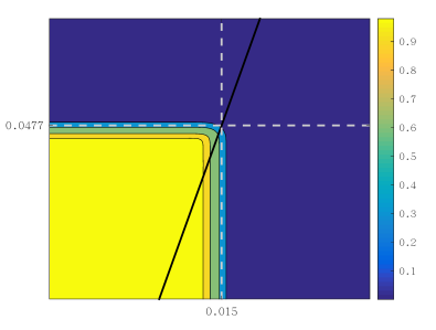
Refer to caption
(a) cosθ0=310subscript𝜃0310\cos\theta_{0}=\dfrac{3}{10}, ctend=0.05𝑐subscript𝑡end0.05ct_{\text{end}}=0.05
Refer to caption
(b) cosθ0=310subscript𝜃0310\cos\theta_{0}=\dfrac{3}{10}, ctend=0.1𝑐subscript𝑡end0.1ct_{\text{end}}=0.1
Refer to caption
(c) cosθ0=310subscript𝜃0310\cos\theta_{0}=\dfrac{3}{10}, ctend=0.2𝑐subscript𝑡end0.2ct_{\text{end}}=0.2
Refer to caption
(d) cosθ0=610subscript𝜃0610\cos\theta_{0}=\dfrac{6}{10}, ctend=0.05𝑐subscript𝑡end0.05ct_{\text{end}}=0.05
Refer to caption
(e) cosθ0=610subscript𝜃0610\cos\theta_{0}=\dfrac{6}{10}, ctend=0.1𝑐subscript𝑡end0.1ct_{\text{end}}=0.1
Refer to caption
(f) cosθ0=610subscript𝜃0610\cos\theta_{0}=\dfrac{6}{10}, ctend=0.2𝑐subscript𝑡end0.2ct_{\text{end}}=0.2
Refer to caption
(g) cosθ0=910subscript𝜃0910\cos\theta_{0}=\dfrac{9}{10}, ctend=0.05𝑐subscript𝑡end0.05ct_{\text{end}}=0.05
Refer to caption
(h) cosθ0=910subscript𝜃0910\cos\theta_{0}=\dfrac{9}{10}, ctend=0.1𝑐subscript𝑡end0.1ct_{\text{end}}=0.1
Refer to caption
(i) cosθ0=910subscript𝜃0910\cos\theta_{0}=\dfrac{9}{10}, ctend=0.2𝑐subscript𝑡end0.2ct_{\text{end}}=0.2
Figure 1: Profile of E0subscript𝐸0E_{0} of the inflow problem with the HMP2𝐻𝑀subscript𝑃2{H\!M\!P}_{2} model, where the directions are different

In order to validate the capability of the 3D HMPN𝐻𝑀subscript𝑃𝑁{H\!M\!P}_{\!N} model to simulate Dirac delta functions in any direction, we choose some different 𝛀0subscript𝛀0\bm{\Omega}_{0}, with 𝛀0=(cosθ0,sinθ0)subscript𝛀0subscript𝜃0subscript𝜃0\bm{\Omega}_{0}=(\cos\theta_{0},\sin\theta_{0}), and cosθ0=310subscript𝜃0310\cos\theta_{0}=\dfrac{3}{10}, 610610\dfrac{6}{10}, and 910910\dfrac{9}{10}. We simulate this problem with the 3D HMPN𝐻𝑀subscript𝑃𝑁{H\!M\!P}_{\!N} model till ctend=0.05,0.1𝑐subscript𝑡end0.050.1ct_{\text{end}}=0.05,0.1, and 0.20.20.2, with N=2𝑁2N=2. Nx=Ny=160subscript𝑁𝑥subscript𝑁𝑦160N_{x}=N_{y}=160 is applied in this example. The results of the contours of E0acsubscript𝐸0𝑎𝑐\dfrac{E_{0}}{ac} are presented in Figure 1. The black line represents the direction of 𝛀0subscript𝛀0\bm{\Omega}_{0}, i.e. the slope of each line is tanθ0subscript𝜃0\tan\theta_{0}, and the dashed lines (x=ctendcosθ0𝑥𝑐subscript𝑡endsubscript𝜃0x=ct_{\text{end}}\cos\theta_{0} and y=ctendsinθ0𝑦𝑐subscript𝑡endsubscript𝜃0y=ct_{\text{end}}\sin\theta_{0}) figure out the theoretical results of the wave in x𝑥x-direction and y𝑦y-direction, respectively. From the results, one can conclude that the 3D HMPN𝐻𝑀subscript𝑃𝑁{H\!M\!P}_{\!N} model can capture the wave well. Therefore, the approximation of the HMPN𝐻𝑀subscript𝑃𝑁{H\!M\!P}_{\!N} to the delta function in any direction is satisfying.

Gaussian source problem

This example is to show the rotational invariance of the MPN𝑀subscript𝑃𝑁{M\!P}_{\!N} model. The initial specific intensity is a Gaussian distribution in space [23]:

I0(𝒙;𝛀)=14πac2πθe𝒙22θ,θ=1100,𝒙(L,L)×(L,L).formulae-sequencesubscript𝐼0𝒙𝛀14𝜋𝑎𝑐2𝜋𝜃superscript𝑒superscriptnorm𝒙22𝜃formulae-sequence𝜃1100𝒙𝐿𝐿𝐿𝐿\displaystyle I_{0}(\bm{x};\bm{\Omega})=\dfrac{1}{4\pi}\dfrac{ac}{\sqrt{2\pi\theta}}e^{-\frac{\|\bm{x}\|^{2}}{2\theta}},\quad\theta=\frac{1}{100},\quad\bm{x}\in(-L,L)\times(-L,L). (5.14)

Here the computational domain is set by L=1𝐿1L=1, and ctend=0.5𝑐subscript𝑡end0.5ct_{\text{end}}=0.5 so that that the energy reaching the boundaries is negligible, and vacuum boundary conditions are prescribed at all the boundaries. The medium is purely scattering with σs=σt=1subscript𝜎𝑠subscript𝜎𝑡1\sigma_{s}=\sigma_{t}=1, thus the material coupling term vanishes. We also set the external source to be zero.

Refer to caption
(a) N=2𝑁2N=2
Refer to caption
(b) N=3𝑁3N=3
Refer to caption
(c) N=4𝑁4N=4
Figure 2: Profile of E0subscript𝐸0E_{0} of the Gassian source problem with the HMPN𝐻𝑀subscript𝑃𝑁{H\!M\!P}_{\!N} model

We use 400×400400400400\times 400 cells to simulate this problem, with the HMP2𝐻𝑀subscript𝑃2{H\!M\!P}_{2} model, the HMP3𝐻𝑀subscript𝑃3{H\!M\!P}_{3} model, and the HMP4𝐻𝑀subscript𝑃4{H\!M\!P}_{4} model, and the results are presented in Figure 2, from which one can conclude the contours of the E0acsubscript𝐸0𝑎𝑐\dfrac{E_{0}}{ac} are circles and there is no ray effect. This validates the rotational invariance of the 3D HMPN𝐻𝑀subscript𝑃𝑁{H\!M\!P}_{\!N} model.

Bilateral inflow problem

In the previous numerical example, we validate the capability of the 3D HMPN𝐻𝑀subscript𝑃𝑁{H\!M\!P}_{\!N} model to simulate Dirac delta function. In this example, we show that the 3D HMPN𝐻𝑀subscript𝑃𝑁{H\!M\!P}_{\!N} model can also approximate isotropic distribution function.

We use the RTE without right hand side (5.13), and the initial state is chosen as

I0(𝒙;𝛀)={acδ(𝛀𝛀0),x<210 and y<210,ac4π,x>210 and y>210,1034πac,otherwise,I_{0}(\bm{x};\bm{\Omega})=\left\{\begin{aligned} &ac\delta(\bm{\Omega}-\bm{\Omega}_{0}),\quad&x<-\dfrac{2}{10}\text{ and }y<-\dfrac{2}{10},\\ &\dfrac{ac}{4\pi},\quad&x>\dfrac{2}{10}\text{ and }y>\dfrac{2}{10},\\ &\dfrac{10^{-3}}{4\pi}ac,\quad&\text{otherwise},\end{aligned}\right.

where 𝛀0=(22,22)Tsubscript𝛀0superscript2222𝑇\bm{\Omega}_{0}=(\frac{\sqrt{2}}{2},\frac{\sqrt{2}}{2})^{T}. In the bottom-left region, the distribution function is a Dirac delta function, which is extremely anisotropic and hard to approximate with the PNsubscript𝑃𝑁P_{N} model, which approximates the specific intensity with polynomials. Meanwhile, in the upper-right region, the distribution function is a constant with respect to the velocity direction 𝛀𝛀\bm{\Omega}, which is isotropic. Generally, it is challenging to get a good approximation on a Dirac delta function and a constant function.

The computational domain is [1,1]×[1,1]1111[-1,1]\times[-1,1], and the infinite boundary conditions are prescribed at the boundaries. We simulate this problem with the MPN𝑀subscript𝑃𝑁{M\!P}_{\!N} model and the PNsubscript𝑃𝑁P_{N} model till ctend=0.1𝑐subscript𝑡end0.1ct_{\text{end}}=0.1 with N=2𝑁2N=2, 333, and 444. Nx=Ny=400subscript𝑁𝑥subscript𝑁𝑦400N_{x}=N_{y}=400 is applied in this example.
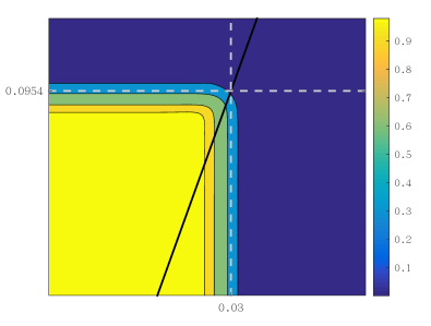
Refer to caption
(a) HMP2𝐻𝑀subscript𝑃2{H\!M\!P}_{2} model
Refer to caption
(b) P2subscript𝑃2P_{2} model
Refer to caption
(c) E0subscript𝐸0E_{0} when y=x𝑦𝑥y=x
Refer to caption
(d) HMP3𝐻𝑀subscript𝑃3{H\!M\!P}_{3} model
Refer to caption
(e) P3subscript𝑃3P_{3} model
Refer to caption
(f) E0subscript𝐸0E_{0} when y=x𝑦𝑥y=x
Refer to caption
(g) HMP4𝐻𝑀subscript𝑃4{H\!M\!P}_{4} model
Refer to caption
(h) P4subscript𝑃4P_{4} model
Refer to caption
(i) E0subscript𝐸0E_{0} when y=x𝑦𝑥y=x
Figure 3: Profile of E0subscript𝐸0E_{0} of the bilateral inflow with the HMP2𝐻𝑀subscript𝑃2{H\!M\!P}_{2} model and the P2subscript𝑃2P_{2} model

In Figure 3, we present the E0subscript𝐸0E_{0} of the 3D HMPN𝐻𝑀subscript𝑃𝑁{H\!M\!P}_{\!N} model and the PNsubscript𝑃𝑁P_{N} model for N=2𝑁2N=2, 333, and 444, and additionally, we present the E0acsubscript𝐸0𝑎𝑐\dfrac{E_{0}}{ac} of these two models along the line y=x𝑦𝑥y=x. According to the results in Figure 3, we can conclude that in the upper-right region, for this constant function, the HMPN𝐻𝑀subscript𝑃𝑁{H\!M\!P}_{\!N} model and the PNsubscript𝑃𝑁P_{N} model gets similar results, i.e. these two models can approximate this kind of isotropic function well. However, in the bottom-left region, for this Dirac delta function, the HMPN𝐻𝑀subscript𝑃𝑁{H\!M\!P}_{\!N} model gets a good approximation, but there are unphysical oscillations in the results of the PNsubscript𝑃𝑁P_{N} model. In particular, due to these unphysical oscillations, along the line y=x𝑦𝑥y=x, E0acsubscript𝐸0𝑎𝑐\dfrac{E_{0}}{ac} of the PNsubscript𝑃𝑁P_{N} model can be even greater than 111. Therefore, one can conclude that the HMPN𝐻𝑀subscript𝑃𝑁{H\!M\!P}_{\!N} model can not only get a good approximate on an isotropic distribution function, but also approximate the Dirac delta function well.

Lattice problem

The lattice problem is a checkerboard of highly scattering and highly absorbing regions loosely based on a small part of a lattice core. The computational domain is [0,7]×[0,7]0707[0,7]\times[0,7], divided into 49 grids in Figure 4. In the red grids and the black grid, the absorbing and scattering coefficients are 0 and 1 respectively. In the white grids, the absorption and scattering are 10 and 0, respectively. The external source s𝑠s is set as ac𝑎𝑐ac in the black grid, and 0 in other grids. The initial state is set as I=108ac𝐼superscript108𝑎𝑐I=10^{-8}ac, and vacuum boundary condition are prescribed on all boundaries.
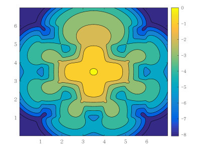
Figure 4: Computational domain of the lattice problem
Refer to caption
(a) N=2𝑁2N=2
Refer to caption
(b) N=4𝑁4N=4
Refer to caption
(c) N=6𝑁6N=6
Figure 5: Profile of E0subscript𝐸0E_{0} of the lattice problem with the HMPN𝐻𝑀subscript𝑃𝑁{H\!M\!P}_{\!N} model

We simulate this problem with the HMPN𝐻𝑀subscript𝑃𝑁{H\!M\!P}_{\!N} model with N=2𝑁2N=2, 444, and 666 till ctend=3.2𝑐subscript𝑡end3.2ct_{\text{end}}=3.2, the number of grids is 200×200200200200\times 200, and the results of log10E0acsubscript10subscript𝐸0𝑎𝑐\log_{10}\dfrac{E_{0}}{ac} are presented in Figure 5. According to the results, the HMPN𝐻𝑀subscript𝑃𝑁{H\!M\!P}_{\!N} model gives a satisfying result, and the result of E0subscript𝐸0E_{0} is always positive in this problem.

6 Conclusion

The 3D HMPN𝐻𝑀subscript𝑃𝑁{H\!M\!P}_{\!N} model was derived as a reduced nonlinear model for RTE in 3D space. The model is hopeful to capture both very singular specific intensity as Dirac delta function and very regular specific intensity as constant function. The model has some mathematical advantages, including global hyperbolicity, rotational invariance, physical wave speeds, spectral accuracy, and correct higher-order Eddington approximation. We validated the new model by some preliminary numerical results. In the following, we will try to apply the model to some practical problems.

Acknowledgements

The authors are partially supported by Science Challenge Project, No. TZ2016002, the CAEP foundation (No. CX20200026), and the National Natural Science Foundation of China (Grant No. 91630310 and 11421110001, 11421101).

References

  • [1] E. Abdikamalov, A. Burrows, C. D. Ott, F. Löffler, E. O’Connor, J. C. Dolence, and E. Schnetter. A new Monte Carlo method for time-dependent neutrino radiation transport. The Astrophysical Journal, 755(2):111, 2012.
  • [2] G. W. Alldredge, R. Li, and W. Li. Approximating the M2subscript𝑀2M_{2} method by the extended quadrature method of moments for radiative transfer in slab geometry. Kinetic & Related Models, 9(2), 2016.
  • [3] G. Bird. Molecular Gas Dynamics and the Direct Simulation of Gas Flows. Oxford: Clarendon Press, 1994.
  • [4] J. E. Broadwell. Study of rarefied shear flow by the discrete velocity method. Journal of Fluid Mechanics, 19(03):401–414, 1964.
  • [5] T. A. Brunner. Forms of approximate radiation transport. Tech. Rep SAND2002-1778, 2002.
  • [6] T. A. Brunner and J. P. Holloway. One-dimensional Riemann solvers and the maximum entropy closure. Journal of Quantitative Spectroscopy and Radiative Transfer, 69(5):543–566, 2001.
  • [7] T. A. Brunner and J. P. Holloway. Two-dimensional time dependent Riemann solvers for neutron transport. Journal of Computational Physics, 210:386–399, 2005.
  • [8] Z. Cai, Y. Fan, and R. Li. Globally hyperbolic regularization of Grad’s moment system in one dimensional space. Comm. Math. Sci., 11(2):547–571, 2013.
  • [9] Z. Cai, Y. Fan, and R. Li. Globally hyperbolic regularization of Grad’s moment system. Comm. Pure Appl. Math., 67(3):464–518, 2014.
  • [10] Z. Cai, Y. Fan, and R. Li. A framework on moment model reduction for kinetic equation. SIAM J. Appl. Math., 75(5):2001–2023, 2015.
  • [11] Z. Cai, Y. Fan, R. Li, and Z. Qiao. Dimension-reduced hyperbolic moment method for the Boltzmann equation with BGK-type collision. Commun. Comput. Phys., 15(5):1368–1406, 2014.
  • [12] Z. Cai, R. Li, and Z. Qiao. Globally hyperbolic regularized moment method with applications to microflow simulation. Computers and Fluids, 81:95–109, 2013.
  • [13] B. Davison. On the rate of convergence of the spherical harmonics method for the plane case, isotropic scattering. Canadian Journal of Physics, 38(11):1526–1545, 1960.
  • [14] J. D. Densmore, K. G. Thompson, and T. J. Urbatsch. A hybrid transport-diffusion Monte Carlo method for frequency-dependent radiative-transfer simulations. Journal of Computational Physics, 231(20):6924–6934, 2012.
  • [15] B. Dubroca and J. Feugeas. Theoretical and numerical study on a moment closure hierarchy for the radiative transfer equation. Comptes Rendus de l’Academie des Sciences Series I Mathematics, 329(10):915–920, 1999.
  • [16] J. J. Duderstadt and W. R. Martin. Transport theory. Wiley, New York, 1979.
  • [17] Y. Fan, J. An, and L. Ying. Fast algorithms for integral formulations of steady-state radiative transfer equation. Journal of Computational Physics, 380:191–211, 2019.
  • [18] Y. Fan, J. Koellermeier, J. Li, R. Li, and M. Torrilhon. Model reduction of kinetic equations by operator projection. Journal of Statistical Physics, 162(2):457–486, 2016.
  • [19] Y. Fan, R. Li, and L. Zheng. A nonlinear hyperbolic model for radiative transfer equation in slab geometry. arXiv preprint arXiv:1911.05472, 2019.
  • [20] Y. Fan, R. Li, and L. Zheng. A nonlinear moment model for radiative transfer equation in slab geometry. Journal of Computational Physics, 404:109128, 2020.
  • [21] J. Fleck and J. Cummings. An implicit Monte Carlo scheme for calculating time and frequency dependent nonlinear radiation transport. J. Comput. Phys., 8(3):313–342, 1971.
  • [22] C. Hauck and R. McClarren. Positive PNsubscript𝑃𝑁P_{N} closures. SIAM Journal on Scientific Computing, 32(5):2603–2626, 2010.
  • [23] C. D. Hauck, M. Frank, and E. Olbrant. Perturbed, entropy-based closure for radiative transfer. SIAM Journal on Applied Mathematics, 6(3):557–587, 2013.
  • [24] C. K. Hayakawa, J. Spanier, and V. Venugopalan. Coupled forward-adjoint Monte Carlo simulations of radiative transport for the study of optical probe design in heterogeneous tissues. SIAM Journal on Applied Mathematics, 68(1):253–270, 2007.
  • [25] J. H. Jeans. Stars, gaseous, radiative transfer of energy. Monthly Notices of the Royal Astronomical Society, 78:28–36, 1917.
  • [26] A. D. Klose, U. Netz, J. Beuthan, and A. H. Hielscher. Optical tomography using the time-independent equation of radiative transfer—part 1: forward model. Journal of Quantitative Spectroscopy and Radiative Transfer, 72(5):691–713, 2002.
  • [27] R. Koch and R. Becker. Evaluation of quadrature schemes for the discrete ordinates method. Journal of Quantitative Spectroscopy and Radiative Transfer, 84(4):423–435, 2004.
  • [28] E. W. Larsen and J. E. Morel. Advances in discrete-ordinates methodology. In Nuclear Computational Science, pages 1–84. Springer, 2010.
  • [29] C. D. Levermore. Moment closure hierarchies for kinetic theories. Journal of Statistical Physics, 83(5-6):1021–1065, 1996.
  • [30] R. Li, W. Li, and L. Zheng. A nonlinear three-moment model for radiative transfer in spherical symmetry. Mathematics and Computers in Simulation, 170:285 – 299, 2020.
  • [31] A. Marshak and A. Davis. 3D radiative transfer in cloudy atmospheres. Springer Science & Business Media, 2005.
  • [32] G. D. Maso, P. G. LeFloch, and F. Murat. Definition and weak stability of nonconservative products. J. Math. Pures Appl., 74(6):483–548, 1995.
  • [33] R. G. McClarren, T. M. Evans, R. B. Lowrie, and J. D. Densmore. Semi-implicit time integration for PNsubscript𝑃𝑁P_{N} thermal radiative transfer. Journal of Computational Physics, 227(16):7561–7586, 2008.
  • [34] R. G. McClarren, J. P. Holloway, and T. A. Brunner. On solutions to the Pnsubscript𝑃𝑛P_{n} equations for thermal radiative transfer. Journal of Computational Physics, 227(5):2864–2885, 2008.
  • [35] D. Mihalas. Stellar Atmospheres. San Francisco, WH Freeman and Co., 650p, 1978.
  • [36] G. N. Minerbo. Maximum entropy eddington factors. Journal of Quantitative Spectroscopy and Radiative Transfer, 20(6):541–545, 1978.
  • [37] G. Pomraning. The equations of radiation hydrodynamics. Pergamon Press, 1973.
  • [38] S. Rhebergen, O. Bokhove, and J. J. W. van der Vegt. Discontinuous Galerkin finite element methods for hyperbolic nonconservative partial differential equations. J. Comput. Phys., 227(3):1887–1922, 2008.
  • [39] K. Stamnes, S.-C. Tsay, W. Wiscombe, and K. Jayaweera. Numerically stable algorithm for discrete-ordinate-method radiative transfer in multiple scattering and emitting layered media. Appl. Opt., 27(12):2502–2509, Jun 1988.
  • [40] T. Tarvainen, M. Vauhkonen, V. Kolehmainen, and J. P. Kaipio. Hybrid radiative-transfer–diffusion model for optical tomography. Applied optics, 44(6):876–886, 2005.