Efficient Pig Counting in Crowds with Keypoints Tracking and Spatial-aware Temporal Response Filtering

Abstract

Pig counting is a crucial task for large-scale pig farming, which is usually completed by human visually. But this process is very time-consuming and error-prone. Few studies in literature developed automated pig counting method. Existing methods only focused on pig counting using single image, and its accuracy is challenged by several factors, including pig movements, occlusion and overlapping. Especially, the field of view of a single image is very limited, and could not meet the requirements of pig counting for large pig grouping houses. To that end, we presented a real-time automated pig counting system in crowds using only one monocular fisheye camera with an inspection robot. Our system showed that it produces accurate results surpassing human. Our pipeline began with a novel bottom-up pig detection algorithm to avoid false negatives due to overlapping, occlusion and deformation of pigs. A deep convolution neural network (CNN) is designed to detect keypoints of pig body part and associate the keypoints to identify individual pigs. After that, an efficient on-line tracking method is used to associate pigs across video frames. Finally, a novel spatial-aware temporal response filtering (STRF) method is proposed to predict the counts of pigs, which is effective to suppress false positives caused by pig or camera movements or tracking failures. The whole pipeline has been deployed in an edge computing device, and demonstrated the effectiveness.

I INTRODUCTION

Frequently counting the number of pigs in grouping houses is a critical management task for large-scale pig farming facilities. On one hand, pigs are often moved into different barns at distinct growth stages or grouped into separate large pens by size. Farmers need to know how many pigs are in each large pens. On the other hand, comparing the counting result with the actual number of pigs enables the early detection of unexpected events, e.g., missing pigs. However, walking around the pig barns to count a large number of pigs is costly in labor. Thus, automated pig counting and monitoring using computer vision techniques is a promising way to support intensive pig farming management, while reducing cost.

Figure 1: Illustrations of pig counting challenges in large grouping houses. The top-down view images are captured by our inspection robot with a fisheye camerat. Red arrows point to examples of pig overlapping and occlusion. Yellow arrows show cases where pigs are moving in or out of camera field of view.

Figure 2: Illustrations of our pig counting system. (a) the installed inspection robots with rails and fisheye cameras for pig counting. (b) a single video frame with detected pig skeletons using our counting algorithm.

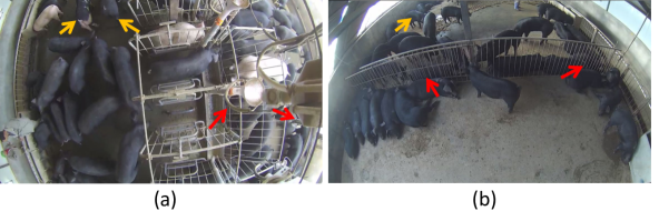
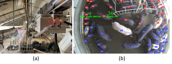
In recent years, various computer vision algorithms have been widely adopted to support various developments of agriculture and farming automation, such as cattle gait tacking [3], pig weight estimation [12] and fruit counting [9]. Despite of these exciting progresses, pig counting remains a very challenging task, due to large pig movements, high group density, overlapping, occlusion and camera perspective, as illustrated in Fig. 1. Few works in literature studied the development of automated pig counting system. Existing works [19] only handled pig counting problem in a single image. Nonetheless, as shown in Fig. 1, the field of view of a single image is only restricted to a small region and it is impossible to monitor a large pig grouping house. Furthermore, it could not deal with the cases that pigs frequently enter into or exist from the camera view. Towards overcoming these challenges, we presented an novel automated counting algorithm with an inspection robot and monocular fisheye camera. Fig. 2a showed two pictures of our inspection robot with a fisheye camera installed on the roof rail in our experimental pig grouping houses. Fig. 2b visualized a single video frame with detected pig skeletons output using our pig counting pipeline.

Figure 3: Pig counting pipeline. The inspection robot moved from one side of the pig house roof to the other end to scan the whole region. A proposed bottom-up detection CNN model was first applied on each video frame to obtain the keypoints and skeletons of all pig candidates. An on-line tracking algorithm was then used to generate the temporal associations across frames. Lastly, STRF, including spatial encoding and temporal filtering, was used to generate the final count.

The main contributions of this paper are summarized as follows. 1) The sensor configuration is presented, which is suitable for pig counting in large-scale grouping house. 2) A novel bottom-up detection method is proposed to identify pigs, while addressing detection challenges due to overlapping, occlusion and deformation of body shapes. 3) A novel online spatial-aware temporal response filtering (STRF) method is designed to suppress false positives caused by tracking failures or pig movements. 4) An efficient algorithm of the counting pipeline is designed and deployed to an embedded system, which achieves high speed performance.

II RELATED WORK

Counting in the crowd is an important, but challenging task due to severe occlusion, perspective distortions, complex illumination and diverse distribution of target sizes [17]. Recently, deep-learning-based methods [17, 18] have been developed to estimate single image density map for crowd counting. Sindagi et. al. [18] developed a contextual pyramid convolutional neural network (CNN) for crowd density map estimation. Both global and local contexts were employed in the network to achieve better accuracy. Shen et. al. [17] proposed an adversarial cross-scale consistency pursuit method to improve the estimation consistency and reduce the averaging effect in [18]. These methods formulate the counting problem as density map estimation, thus having the advantage to handle server occlusion and perspective distortions. However, density-map-based methods lost the detailed individual information and discarded the accurate location information for each single target. Therefore, it loses the ability to associate targets across time, and is not suitable for video-based counting.

Recently, researchers in agriculture presented many works towards tackling counting problems in various scenarios. Tian et. al. [19] counted pigs in a single image using a CNN-based method for pig density map estimation. Similar as [18], this method is not suitable for video-based counting problem. As a single image only have a small field of view (as shown in Fig. 1), it cannot be used for pig counting in large grouping houses. Liu et. al. [9, 8] developed a fruit counting pipeline using a monocular camera. Individual fruits are first segmented using a CNN-based method, and then tracked by a Kalman Filter corrected Kanade-Lucas-Tomasi (KLT) tracker. A structure from motion (SfM) algorithm was utilized to get the relative 3D location and size estimate to reject outliers and double counted fruit tracks. This method is only suitable for rigid shape and stationary target counting task, and does not work for moving livestock counting cases. Hodgson et. al. [4] demonstrated that images collected by unmanned aerial vehicles (UAV) could help wildlife monitoring and counting. Rivas et. al. [15] studied cattle detection from aerial view photos. Counting based on aerial view is promising, but could hardly be used for indoor livestock counting scenes without developing algorithms to handle severe occlusion (e.g. caused by indoor building structures or perspective distortions), overlapping, double counted tracking trajectories due to entering into or existing from camera view.

Different from previous approaches, we presented a novel video-based pig counting system for large pig grouping houses. The developed counting pipeline overcame dense detection challenges (e.g. overlapping or occlusion) by a novel bottom-up pig body parts detection and association algorithm. A STRF method was developed to obtain the counting number by reducing the counting error caused by tracking failures or pig movements.

III APPROACH

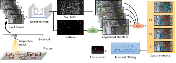
In this work, we presented an efficient pig counting system for large pig grouping houses. Fig. 3 demonstrates the entire algorithm pipeline. In our counting system, the camera moved from one side of the pig grouping house roof till the other end of roof and scanned the whole house with top-down view. A whole single counting pass scanned the house once by the camera. As summarized in the Fig. 3, subsequently, we detected multiple pig body keypoints, associated them to localize each individual pig, tracked pigs cross frames and obtained counting results using STRF method.

III-A SENSOR CONFIGURATION

An inspection robot, which can move back and forth along a rail installed on the roof of the pig house, was used for pig counting data acquisition and processing from top-down view (Fig. 2a). Several sensors used for different applications were installed inside the robot, including a monocular fisheye camera for pig counting, a RGB-D camera for pig weight estimation, gas and temperature sensors for environmental control etc. Inside the inspection robot, an embedded system with RockChip RK3399 multi-core ARM processor was used for processing data from cameras and running the pig counting algorithm.

III-B BOTTOM-UP DETECTION

Figure 4: Illustration of top-down bounding boxes v.s. bottom-up keypoints for pigs detection. Column 1 (C1): bounding boxes had very high overlap ratios for adjacent pigs. Column 2 (C2): body parts keypoints for adjacent pigs. In this work, five keypoints are defined: one middle body part keypoint, two body end keypoints and two quarter body keypoints.

Figure 5: The proposed bottom-up keypoints detection CNN architecture. The network contains two regular convolutional layer at the two ends and 24 depthwise separeble conv. blocks in-between. In (b) the numbers indicate the number of output channels; And $s2$ means a stride of 2. All the conv. layers except the pointwise conv layers have kernel size 3 $\times$ 3.

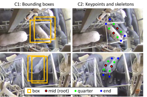
The first step was to detect pig candidates in each video frame. Traditionally, top-down object detectors, such as faster RCNN[14], SSD [7] and YOLOv3 [13], have been widely used. These methods first proposed locations of detection candidates using bounding boxes, and then classified each box to be the real target or not. Non-maximum suppression (NMS) are employed as a post-processing method to significantly reduce false positive candidates by removing the bounding boxes that have high overlap ratios (intersection over union) with each other. Nonetheless, using bounding boxes to localize the pigs is sub-optimal in this application. The deformable long oval pig shapes are very challenging for bounding-box-based approaches in crowded scene. As shown in Fig. 4C1, the bounding boxes around two adjacent pigs have very high overlap ratio, whose ambiguous nature tends to confuse the neural network training. Moreover for inference, the NMS post-processing step would enforce the detector to only select one bounding box for these high overlapping cases, resulting in false negatives. Compared with bounding boxes, the pig skeletons defined by keypoints are more suitable for differentiating pigs in the crowd as shown in Fig. 4C2. In this work, we defined five pig body keypoints, including one mid point (red), two quarter points (green) and two end points (blue); and tree-structured pig skeletons connecting the adjacent keypoints.

Figure 6: Illustration of STRF method. (a) spatial encoding defined activated zone and deactivated zone, and an activity scanning line. (b) Activity scanning line moved with the camera to scan the whole pig house. (c) An example of pig tracking trajectory with count $1$. (c) An example of count $-1$ pig tracking trajectory. (d)(e)(f) Examples of count $0$ tracking trajectory.

Inspired by [2], we presented an efficient bottom-up detection approach (Fig. 5) to overcome aforementioned limitations. This method is consisted of a keypoints detection step and a keypoints association step. These steps were based on a deep convolutional encoder-decoder network. The network output two different kinds of maps: 1) Four keypoint heatmaps and 2) an offset vector field. (Fig. 5d) Each heatmap provided information to classify each pixel into to one of the keypoints or background class. The offset vector field indicated the relative positional relationships between the adjacent keypoints, which helped the system group the keypoints and identify which pig instance that these keypoints belonged to.

Keypoint detection The goal is to detect all visible keypoints belonging to each single pig in the input. For this purpose, we applied a fully convolutional network to produce heatmaps with four channels (three channels for each keypoint type and one for background), which had the same size with the input image. This heatmap prediction was then formulated as a per-pixel multi-class classification problem. For each pixel location, the neural network learned to predict if it belonged to one of the keypoint type or background. We followed [11] to generate classification targets. Let $\mathcal{D}_{R}(y)~{}=~{}\{x:\left\|x-y\right\|<R\}$ be a circular region centered at position $y$ with radius $R$. We denoted $k_{i,c}$ as the $i$-th keypoint of type $c$. All pixels of $\mathcal{D}_{R}(k_{i,c})$ had the same class label $c$. In this work, $R$ was set to be 5. Cross-entropy loss was employed for this task. At testing stage, the local maxima of the heatmaps were chosen as the predicted keypoints.

Keypoint association Due to instance-agnostic nature of the predicted keypoints on heatmaps, one unique instance ID had to be assigned for each detected keypoint so that we ”connect the dots” belonging to the same individual instance. For this purpose, we added to our neural network a separate two channel outputs of offset field indicating the displacement from a given keypoint to its parent in the skeleton (Fig. 4C2). Here we denoted $F(k_{i,c})$ as the parent node of keypoint $k_{i,c}$. If $x\in\mathcal{D}_{R}(k_{i,c})$, the target offset $V(x)$ was vector starting from $x$. If $k_{i,c}$ itself is a root node, i.e. $c=mid$, $V(x)$ ended at $k_{i,c}$; Otherwise $V(x)$ ended at $F(k_{i,c})$.

Let us denote the offset field predicted by the network as $U(x)$. In order to supervise the training, the regression loss for offset field was defined as

$$L_{r}=\sum_{x}(1-G_{0}(x))\left\|U(x)-V(x)\right\|^{2},$$ (1)

where $G_{0}(x)$ was the binary background mask used for ignoring the regression loss at the background pixels, where the offset vector were undefined.

At testing stage, an iterative greedy algorithm was adopt to associate the predicted keypoints. We alternatively searched the best candidate parent node for all the predicted keypoints, and removed the surplus keypoints from their candidate children list, until no better hypothesis could be found. The best candidate parent node was defined as the keypoint which was in the correct class and match the predicted offset vector best. The euclidean distance between the predicted offset and the actual offset was used to measure the match.

Architecture of the network We proposed an architecture (Fig. 5b) for the network. Depthwise separable convolutions [5] were used as the basic building blocks to reduce the computational cost. Following [1], we used location-withheld maxpooling to improve the localization accuracy, which preserved indices at the max pooling layers of the encoder and passed them to the corresponding up-sampling layers of the decoder.

TABLE I: Comparison of keypoint detection results.

Metric	PDJ@0.1			PDJ@0.2			FLOPs	Parameters
Keypoint type	mid	quarter	end	mid	quarter	end
UNet [16]	0.938	0.935	0.895	0.971	0.980	0.953	23G	42M
Hourglass [10]	0.913	0.905	0.866	0.954	0.968	0.932	23G	3.6M
Ours	0.962	0.964	0.934	0.991	0.992	0.978	15G	3.3M

III-C KEYPOINTS TRACKING

In order to count pigs across video frames, an efficient on-line tracking method was employed to associate pig keypoints temporally. This method took the grouped pig keypoints for single frames as input, and then assigned a unique identification number (id) to each pig across frames. This problem was formulated as a bipartite graph matching based energy maximization problem. The estimated pig candidates $C^{t}$ at frame $t$ were then associated with the previous pig candidates $C^{t-1}$ at frame $t-1$ by bipartite graph matching.

$$\begin{split}\widehat{s}=\operatorname*{arg\,max}_{s}\sum_{C_{i}^{t}\in C^{t}}\sum_{C_{j}^{t-1}\in C^{t-1}}\Psi_{C_{i}^{t},C_{j}^{t-1}}\times s_{C_{i}^{t},C_{j}^{t-1}}\\ s.t.\quad\forall C_{j}^{t-1}\in C^{t-1},\sum_{C_{i}^{t}\in C^{t}}s_{C_{i}^{t},C_{j}^{t-1}}\in\{0,1\},\\ \quad\forall C_{i}^{t}\in C^{t},\sum_{C_{j}^{t-1}\in C^{t-1}}s_{C_{i}^{t},C_{j}^{t-1}}\in\{0,1\},\end{split}$$ (2)

where $C_{j}^{t-1}$ was the $j^{th}$ pig candidate in $C^{t-1}$ and $C_{i}^{t}$ was the $i^{th}$ pig candidate in $C^{t}$. $s_{C_{i}^{t},C_{j}^{t-1}}\in\{0,1\}$ was a binary variable and indicates if $C_{j}^{t-1}$ and $C_{i}^{t}$ were associated. The potential $\Psi_{C_{i}^{t},C_{j}^{t-1}}$ represented the similarity measurements between $C_{j}^{t-1}$ and $C_{i}^{t}$.

$$\Psi_{C_{i}^{t},C_{j}^{t-1}}=\lambda_{1}\Psi^{A}_{C_{i}^{t},C_{j}^{t-1}}+\lambda_{2}\Psi^{L}_{C_{i}^{t},C_{j}^{t-1}},$$ (3)

where $\Psi^{A}_{C_{i}^{t},C_{j}^{t-1}}$ represented the keypoints appearance similarities between candidates. And $\Psi^{L}_{C_{i}^{t},C_{j}^{t-1}}$ implied the spatial similarities. $\lambda_{1}$ and $\lambda_{2}$ were hyper-parameters to balance the contributions of the two terms.

The spatial similarities was calculated as the $l_{2}$ distance between the propagated $C_{j}^{t-1}$ spatial location and encoded $C_{i}^{t}$ center location. $\Psi^{L}_{C_{i}^{t},C_{j}^{t-1}}=\left\|P(L(C_{j}^{t-1}))-L(C_{i}^{t})\right\|^{2}$. The appearance similarity was calculated as the the $l_{2}$ distance across all keypoints embedded deep features between $C_{i}^{t}$ and $C_{j}^{t-1}$.

$$\Psi^{L}_{C_{i}^{t},C_{j}^{t-1}}=\sum_{n=1}^{5}\lambda_{n}^{L}\left\|K^{n}_{C_{j}^{t-1}}-K^{n}_{C_{i}^{t}}\right\|^{2},$$ (4)

where $K^{n}$ represented the $n^{th}$ keypoint deep appearance feature obtained from convolution layer before the last upsampling layer of our keypoints CNN. $\lambda_{n}^{L}$ were the hyper-parameters balancing the weights.

The aforementioned bipartite graph matching problem was solved using Hungarian method.

III-D SPATIAL-AWARE TEMPORAL RESPONSE FILTERING

Traditionally, video-based counting methods [9, 8] counted the number of unique tracklet ID as the final counting results. These methods were suitable for the cases, where the target objects were stationary and object occlusion was very rare. In the large-scale pig counting scenario, however, pigs moved fast in different directions, and the same pig will often walked out of the camera view and came back again. In addition, the indoor building structures (e.g. the feeding machine) would sometimes block large part of the camera view causing severe occlusions. Occlusions across long frames will cause tracking failure, and break trajectory of one single object into two or more. In these cases, counting the number of unique tracklet IDs would suffer from large false positive errors. To overcome these limitations, we represented a novel spatial-aware temporal response filtering (STRF) method to perform on-line counting, while minimizing the false positives.

The STRF took the tracking trajectories for all previous frames as input, and output the final counting number. It consisted of two steps: 1) spatial encoding; and 2) temporal response filtering. The spatial encoding stage processed each video frame independently, and each detected pig candidate in the frame was assigned a code number based on their spatial locations. The temporal response filtering stage examined each candidate’s trajectory across time and obtained a count number, $count_{i}\in\{0,1,-1\}$, for this single candidate. The final counting result was the sum of all count number for all candidates: $\sum_{i=0}^{N}count_{i}$.

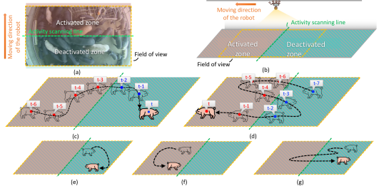
As shown in Fig. 6a, the spatial encoding stage divided one image frame into activated zone and deactivated zone by an activity scanning line. This scanning line was stationary in a single frame, but served to scan the whole pig house moving with the inspection robot. For all detected pig candidates, activity codes will be assigned based on which activity zone these pigs were in. In our work, pigs in activated zone were assigned code value $0$, and pigs in deactivated zone were assigned code value $1$. Deactivated zone indicated that all candidates inside have already been counted by the algorithm; and the candidates in activated zone would be counted when the activity scanning line scanned through them.

In the temporal response filtering step, lists of spatial codes in temporal order were generated for each trajectory. One trajectory had one list of spatial codes, and each element of the list corresponded to a time point. Fig. 6c illustrated one example of one single pig trajectory from time point $t-6$ to time point $t$, where the blue color represented code $1$ and the red color represented code $0$. As it was shown, the generated temporal code was [0, 0, 0, 0, 1, 1, 1] from $t-6$ to $t$. The final count for this trajectory $count_{i}$ was obtained as the sum of the first order difference of the temporal codes. In this case, the count would be $1$, which indicated that this pig was scanned once (from deactivated zone into activated zone) and the total count should be added by $1$. Similarly, Fig. 6d showed a pig trajectory with code [1, 0, 0, 0, 1, 1, 0, 0] and sum of the the first order difference inferred that the count was $-1$. This meant that this pig, which has been counted before, moved from scanned zone to to-be scanned zone. Thus, the total count should minus $1$. This design enabled the algorithm to avoid false positives counting caused by pig movements into/out camera view. Fig. 6e-g showed examples when the pig trajectory count was $0$. Fig. 6e-f represented pig trajectories that never went across the scanning line. Fig. 6g represented cases where the trajectory started and ended in the same activity zone. These examples demonstrated that SFRT would not be influenced by the tracking failures (e.g. broke one trajectory into several cased by occlusion) that happened only in one single zone. In this study, a low-pass filter with window size of 5 was applied before the first order differential calculation. This low-pass filtering step was designed to avoid the trajectory jitter near the activity scanning line. The final counting result for the whole video also added the number of detected candidates in deactivated zone of the beginning frame and the number of detected candidates in activated zone of the ending frame.

IV EXPERIMENTS

We collected 51 videos by inspection robots installed in pig grouping houses of two different pig farming corporations. All videos were originally recorded at 1280$\times$720 resolution with frame rate of 25 $f/s$. For this study, we first resized the video frame to 360$\times$640, and then cropped them to 352$\times$640. All experiments in this work used this resolution. Each video (pig house) had 120$\sim$250 pigs. The length of the videos ranged from 2 minutes to 4 minutes. We randomly split these videos into three subsets, 21 for training, 5 for validation and 25 for testing. The ground truth were provided by workers, who counted the pigs inside the grouping houses when the videos were recorded.

IV-A COMPARISON WITH HUMAN READER

To demonstrate the effectiveness of out method, we compared the performance of our counting system with human readers on test dataset. There were three readers for this study. The readers were required to provide count results by watching the same top-down view videos as the input of the algorithm. There were no time limits for the reading process, and the readers were allowed to pause, rewind, replay the video and took notes for unlimited times. Each reader estimated the pig counts for all the videos in the test datasets. The counting error for both the proposed method and human reader were evaluated using mean absolute percentage error (MAPE) and mean absolute error (MAE). The three readers have MAPE of 11.0%, 17.4%, and 15.9%; and MAE of 12.6, 26.3 and 25.2, respectively. The average time that the human readers have spent on per video is around 1.5 hours. In contrast, our method had MAPE of 2.67%, and MAE of 3.32, which significantly outperformed the human readers.

IV-B ABLATION STUDY

To validate our proposed CNN architecture for keypoints detection, we compared our method with UNet [16] and stacked Hourglass network [10] using the same train, validation and test datasets. Both methods were modified to fit our pixel-level keypoints detection pipelines. Following  [6], the cropping operators was removed from UNet and 7 UNet-submodules were used. The Stacked Hourglass network tested had two hourglass stacked. The Percent of Detected Joints (PDJ) [20] was used as the evaluation metric. One keypoint was considered as detected if the distance between the predicted keypoint and the ground truth was smaller than a fraction of the total length of the skeleton of the pig. As shown in Table  I, our method achieved better keypoints detection accuracy for all 5 body parts with significantly less computation cost and smaller parameter size.

TABLE II: Comparison of pig counting

Method	MAPE	MAE
SSD [7] + Tracking	327%	412
YOLOv3 [13] + Tracking	247%	368
Proposed Keypoint Detector + Tracking	152%	191
SSD [7] + Tracking + STRF	10.1%	12.2
YOLOv3 [13] + Tracking + STRF	5.35%	7.00
Proposed Keypoint Detector + Tracking + STRF	2.67%	3.32

We also compared our bottom-up detection method with SSD [7] and YOLOv3  [13] using top-down bounding boxes detection metric: mean average precision with 0.5 IOU (mAP@0.5). The proposed bottom-up approach did not directly output bounding boxes of pig. Thus, we used keypoints/skeleton bounding boxes instead. It should be noted that the keypoints bounding boxes are more strict and harder to predict, and our network was never trained for the bounding boxes detection task. SSD achieved 73.3% mAP while YOLOv3 achieves 79.7% mAP. Our method had 84.3% mAP. Although more challenging, our method showed better performance. It should be noted that a large part of the detection failures happened around image boudaries where large fisheye distortion and image cutoff happened. Due to the design of STRF methods, most of the failures will not influence the final counting result.

To evaluate the effectiveness of the STRF method, we compared the counting results with and without STRF using our detection method, SSD and YOLOv3, resepctively. Table II showed that the MAPE and MAE are significantly small when using STRF. And our method achieved better performance with/without STRF compared with SSD or YOLOv3.

IV-C RUNTIME ANALYSIS

We analyzed the runtime performance of our method using the test dataset. On desktop computer, it achieved 3.42 frames per second (FPS) running speed with a Intel i7-6850K CPU and 32GB DDR4 2133MHz Memory. When accelerated by a single NVIDIA GeForce GTX 1080Ti GPU, it achieved 82.6 FPS. The proposed counting algorithm has also been deployed on two different edge computing devices. It achieved 0.625 FPS on a Firefly-RK3399 platform, which had a 2GB Memory and a Rockchip RK3399 CPU. On NVIDIA Jetson Nano platform, it achieved 3.19 FPS with a 4GB memory, a quad-core ARM A57 CPU and 128 CUDA cores.

V CONCLUSION

In this work, we presented a hardware configuration and novel efficient algorithm for pig counting in large grouping houses. An inspection robot with a monocular fisheye camera was installed on the roof with rails, along which the root could move back and forth to collect top-down view videos. A novel efficient bottom-up CNN detection approach was developed to first detect pigs from the crowd. Second, a online tracking method was employed to associate pig ID temporally. A novel STRF method was proposed to calculate the final pig counts, while significantly avoid false positive counting due to tracking failure or large pig movements. The low computation cost design significantly reduce the computation time and model size. This counting algorithm has been deployed in edge computing device of the inspection robot, and achieved counting accuracy superior to human readers.

References

- [1] V. Badrinarayanan, A. Kendall, and R. Cipolla. Segnet: A deep convolutional encoder-decoder architecture for image segmentation. IEEE transactions on pattern analysis and machine intelligence, 39(12):2481–2495, 2017.
- [2] Z. Cao, T. Simon, S.-E. Wei, and Y. Sheikh. Realtime multi-person 2d pose estimation using part affinity fields. In Proceedings of the IEEE Conference on Computer Vision and Pattern Recognition, pages 7291–7299, 2017.
- [3] J. Gardenier, J. Underwood, and C. Clark. Object detection for cattle gait tracking. In 2018 IEEE International Conference on Robotics and Automation (ICRA), pages 2206–2213. IEEE, 2018.
- [4] J. C. Hodgson, S. M. Baylis, R. Mott, A. Herrod, and R. H. Clarke. Precision wildlife monitoring using unmanned aerial vehicles. Scientific reports, 6:22574, 2016.
- [5] A. G. Howard, M. Zhu, B. Chen, D. Kalenichenko, W. Wang, T. Weyand, M. Andreetto, and H. Adam. Mobilenets: Efficient convolutional neural networks for mobile vision applications. arXiv preprint arXiv:1704.04861, 2017.
- [6] P. Isola, J.-Y. Zhu, T. Zhou, and A. A. Efros. Image-to-image translation with conditional adversarial networks. In IEEE Conference on Computer Vision and Pattern Recognition, 2017.
- [7] W. Liu, D. Anguelov, D. Erhan, C. Szegedy, S. Reed, C.-Y. Fu, and A. C. Berg. Ssd: Single shot multibox detector. In European conference on computer vision, pages 21–37. Springer, 2016.
- [8] X. Liu, S. W. Chen, S. Aditya, N. Sivakumar, S. Dcunha, C. Qu, C. J. Taylor, J. Das, and V. Kumar. Robust fruit counting: Combining deep learning, tracking, and structure from motion. In 2018 IEEE/RSJ International Conference on Intelligent Robots and Systems (IROS), pages 1045–1052. IEEE, 2018.
- [9] X. Liu, S. W. Chen, C. Liu, S. S. Shivakumar, J. Das, C. J. Taylor, J. Underwood, and V. Kumar. Monocular camera based fruit counting and mapping with semantic data association. IEEE Robotics and Automation Letters, 4(3):2296–2303, 2019.
- [10] A. Newell, K. Yang, and J. Deng. Stacked hourglass networks for human pose estimation. In European conference on computer vision, pages 483–499. Springer, 2016.
- [11] G. Papandreou, T. Zhu, L.-C. Chen, S. Gidaris, J. Tompson, and K. Murphy. Personlab: Person pose estimation and instance segmentation with a bottom-up, part-based, geometric embedding model. In Proceedings of the European Conference on Computer Vision (ECCV), pages 269–286, 2018.
- [12] A. Pezzuolo, M. Guarino, L. Sartori, L. A. González, and F. Marinello. On-barn pig weight estimation based on body measurements by a kinect v1 depth camera. Computers and Electronics in Agriculture, 148:29–36, 2018.
- [13] J. Redmon and A. Farhadi. Yolov3: An incremental improvement. arXiv preprint arXiv:1804.02767, 2018.
- [14] S. Ren, K. He, R. Girshick, and J. Sun. Faster r-cnn: Towards real-time object detection with region proposal networks. In Advances in neural information processing systems, pages 91–99, 2015.
- [15] A. Rivas, P. Chamoso, A. González-Briones, and J. Corchado. Detection of cattle using drones and convolutional neural networks. Sensors, 18(7):2048, 2018.
- [16] O. Ronneberger, P. Fischer, and T. Brox. U-net: Convolutional networks for biomedical image segmentation. In MICCAI, pages 234–241, 2015.
- [17] Z. Shen, Y. Xu, B. Ni, M. Wang, J. Hu, and X. Yang. Crowd counting via adversarial cross-scale consistency pursuit. In Proceedings of the IEEE conference on computer vision and pattern recognition, pages 5245–5254, 2018.
- [18] V. A. Sindagi and V. M. Patel. Generating high-quality crowd density maps using contextual pyramid cnns. In Proceedings of the IEEE International Conference on Computer Vision, pages 1861–1870, 2017.
- [19] M. Tian, H. Guo, H. Chen, Q. Wang, C. Long, and Y. Ma. Automated pig counting using deep learning. Computers and Electronics in Agriculture, 163, 2019.
- [20] A. Toshev and C. Szegedy. Deeppose: Human pose estimation via deep neural networks. In Proceedings of the IEEE conference on computer vision and pattern recognition, pages 1653–1660, 2014.