On the measurement of handedness in Fermi Large Area Telescope data

Abstract

A handedness in the arrival directions of high-energy photons from outside our Galaxy can be related to the helicity of an intergalactic magnetic field. Previous estimates by Tashiro et al. (2014) and Chen et al. (2015) showed a hint of a signal present in the photons observed by the Fermi Large Area Telescope (LAT). An update on the measurement of handedness in Fermi-LAT data is presented using more than 10 years of observations. Simulations are performed to study the uncertainty of the measurements, taking into account the structure of the exposure caused by the energy-dependent instrument response and its observing profile, as well as the background from the interstellar medium. The simulations are required to accurately estimate the uncertainty and to show that previously the uncertainty was significantly underestimated. The apparent signal in the earlier analysis of Fermi-LAT data is rendered non-significant.

1. Introduction

Most of the macrophysical processes around us show no statistical preference of one handedness over the other. A good counterexample are cyclones on a weather map that have a counterclockwise inward spiral in the northern hemisphere and a clockwise one in the southern. These opposite spirals correspond to opposite handednesses, but on average, the number of cyclones in the northern and southern hemispheres are nearly equal, so even in this case, the total or net handedness averages to zero. By contrast, at the microbiological level, for example, there is a global preferred handedness for all life on Earth with amino acids being levorotatory and sugars dextrorotatory (Rothery et al., 2011). Even one of the four fundamental forces in nature – the weak force, responsible for the $\beta$ decay – shows a global preferred handedness. It produces electrons whose spin is anti-parallel to the momentum (Lee & Yang, 1956; Frauenfelder et al., 1957). One then says the electrons are left-handed or have negative chirality, which is the Greek word for handedness.

The examples above illustrate that handedness can manifest itself in a number of different ways. Mathematically, handedness can be related to the existence of a pseudoscalar. Unlike ordinary scalars, which preserve their sign under mirror reflection, pseudoscalars do change their sign under mirror reflection. Similarly, ordinary or polar vectors preserve their direction under mirror reflection, while pseudo or axial vectors change their direction under mirror reflection. An example is the rotation of a car’s axle, which looks reversed in a mirror. Likewise, the curl of a velocity vector, i.e., the vorticity, changes direction, and therefore the dot product of velocity and vorticity also changes its sign in a mirror and is therefore a pseudoscalar. The dot product of the gravity vector on the Earth’s surface and its global angular velocity is also a pseudoscalar. Another example is the magnetic helicity, i.e., the dot product between the magnetic vector potential and its curl, the magnetic field. It plays a particularly important role, because it is a conserved quantity in electrically conducting media (Berger & Field, 1984).

Often, there is a causal connection between different pseudoscalars. For example, gravity in a rotating body can cause finite kinetic and magnetic helicities (Moffatt, 1978). Consider now the skew product

$$Q=(\mbox{\boldmath$n$}{}_{1}\times\mbox{\boldmath$n$}{}_{2})\cdot\mbox{\boldmath$n$}{}_{3}$$ (1)

of three unit vectors $\mbox{\boldmath$n$}{}_{1}$, $\mbox{\boldmath$n$}{}_{2}$, and $\mbox{\boldmath$n$}{}_{3}$ of points on a sphere; see Figure 1 for a sketch showing three patches of increasing size (corresponding to larger energies) at positions $\mbox{\boldmath$n$}{}_{1}$, $\mbox{\boldmath$n$}{}_{2}$, and $\mbox{\boldmath$n$}{}_{3}$ on a left and a right hand. The largest patch corresponds to the palm of the open hand, the intermediate patch corresponds to the fingers, and the smallest patch corresponds to the thumb.​ The two hands lie with their back on the sphere. The cross product $\mbox{\boldmath$n$}{}_{1}\times\mbox{\boldmath$n$}{}_{2}$ of two polar vectors is an axial vector, which points in the direction of $\mbox{\boldmath$n$}{}_{3}$ for the right hand, and in the opposite direction of $\mbox{\boldmath$n$}{}_{3}$ for the left hand. Therefore, $Q$ is positive (negative) for the arrangement of patches on the right (left) hand.

A correspondence between the sign of $Q$ and the sign of magnetic helicity was first proposed by Tashiro & Vachaspati (2013). They demonstrated the possibility of a causal link between the $Q$ product from the photon arrival directions on the celestial sphere and the presence of a large-scale helical magnetic field permeating space even in the voids between galaxy clusters, far from any potential astrophysical sources of magnetic fields.

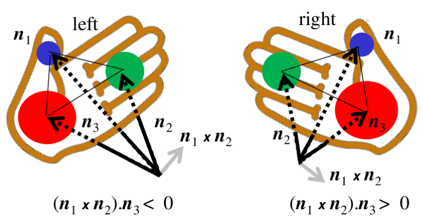
Figure 1.— A sketch showing three patches of increasing size at positions $\mbox{\boldmath$n$}{}_{1}$, $\mbox{\boldmath$n$}{}_{2}$, and $\mbox{\boldmath$n$}{}_{3}$ on a left and a right hand. The largest patch (red) corresponds to the palm of the open hand, the intermediate patch (green) corresponds to the fingers, and the smallest patch (blue) corresponds to the thumb. In this perspective view, the vectors $\mbox{\boldmath$n$}{}_{1}$, $\mbox{\boldmath$n$}{}_{2}$, and $\mbox{\boldmath$n$}{}_{3}$ start at the origins, which lie beneath each of the two hands toward their backsides.

The universality of the significance of this skew product was demonstrated further by Bourdin & Brandenburg (2018), who demonstrated numerically a connection between the sign of magnetic helicity and the sign of the skew product for a triple of magnetic spots on the surface of a sphere such as the Sun. Thus, without necessarily relying on a particular physical motivation for the finiteness of the skew product $Q$ of unit vectors, we wish to examine in the present paper the observational reality of a possible detection.

To illustrate the far-reaching significance of a detection of net handedness, let us mention here the connection between the possibility of a globally helical magnetic field and baryogenesis in the early universe. In fact, there is an epoch in the history of our universe during which the weak force played a crucial role. This is the time of the electroweak phase transition (Vachaspati, 1991, 2001) some $10^{-11}\,{\rm s}$ after the Big Bang, when the temperature was $10^{15}\,{\rm K}$, corresponding to an energy of $100\,{\rm GeV}$, or perhaps before (García-Bellido et al., 2004). At that time, there could have been an excess of left-handed fermions. Fermions and electromagnetic fields couple through the fine structure constant in such a way that the total chirality of fermions and electromagnetic fields does not change. Moreover, the chirality of fermions destabilizes a weak magnetic field and causes it to grow (Joyce & Shaposhnikov, 1997; Boyarsky et al., 2012). This is in principle a promising mechanism for producing magnetic fields of one sign of helicity throughout all of the universe. However, already simple arguments (Brandenburg et al., 2017b) suggested this would only produce magnetic fields of $10^{-18}\,{\rm G}$ normalized to one megaparsec length scale. This might not suffice to explain the lower limit of magnetic field of $10^{-16}\,{\rm G}\,{\rm Mpc}^{-1/2}$ (Neronov & Vovk, 2010), which is implied by the non-detection of secondary photons from the halos of blazars. On the other hand, doubts have been raised regarding the exclusive need to explain this non-detection by a magnetic field of a particular minimum strength (Broderick et al., 2018; Batista et al., 2019). In other words, significant levels of magnetic field may still exist, but the minimum strength cannot reliably be constrained at the present time.

According to the theory of Vachaspati (2001), magnetic field generation may have been accompanied by changes in the Chern-Simon number to generate baryons, which would have implied that the magnetic helicity also changes. It has been shown, however, that the extraordinarily strong departures from thermal equilibrium near the end of inflation (García-Bellido et al., 1999) could have led to magnetic fields several orders of magnitude larger than what can be estimated based on dimensional arguments (Díaz-Gil et al., 2008a, b).

If magnetic fields from the electroweak phase transition are to be responsible for the lower limit of Neronov & Vovk (2010), they must have been helical. This is because only a helical magnetic field would have decayed sufficiently slowly and would have increased its correlation length to kiloparsec scales (Brandenburg et al., 2017a). The helicity of such magnetic fields can manifest itself in at least three possible ways: in parity-odd polarization signals from the cosmic microwave background (Kahniashvili & Ratra, 2005), in primordial gravitational waves (Kahniashvili et al., 2005), and in the propagation properties of energetic photons from blazars that interact with the extragalactic background light (Tashiro et al., 2012).

Using a model of secondary particle emission from blazars, Tashiro et al. (2014) developed a statistic that could be applied to the data from the Fermi Large Area Telescope (LAT). Using the arrival directions of photons from high Galactic latitudes in 60 months of LAT data, they found an indication of left-handedness at the level of 3$\sigma$. Interpreted in their framework, this indicated a left-handed magnetic helicity for the cosmological magnetic field with a field strength of $\sim 10^{-14}$ G on $\sim 10$ Mpc scales. In a follow-up analysis, Chen et al. (2015) also found significant signals that persisted even when accounting for the effect of the LAT energy-dependent exposure. To test this claim, a new analysis is performed using more than 10 years of LAT data with an updated event reconstruction allowing for nearly a doubling of the statistics; see Asplund (2019) for a preliminary account of this work. In addition, simulations are performed to check for the effects of the LAT energy-dependent exposure and the contamination from the interstellar emission. Using these simulations it is found that the measured handedness is not significant.

2. $Q$ Statistic and Data

To look for a signal of handedness in the arrival directions of GeV photons observed with the LAT, the $Q$ statistic developed in Tashiro et al. (2014) is used. The arrival direction of a photon measured to arrive at Galactic longitude and latitude $(l,b)$ is represented by a unit vector in Cartesian coordinates

$$\mbox{\boldmath$n$}{}=(\cos b\cos l,\cos b\sin l,\sin b).$$ (2)

The photons are binned in energy and the bins ordered from low energy to high energy. Let $E_{i}$ denote the photons with observed energies $E_{i,\min}<E<E_{i,\max}$ and say $E_{i}<E_{j}$ if $E_{i,\max}\leq E_{j,\min}$. For any three energy bins, such that $E_{1}<E_{2}<E_{3}$, the $Q$ statistic is calculated as

$$Q(E_{1},E_{2},E_{3},R)=\frac{1}{N_{3}}\sum_{k=1}^{N_{3}}\left(\bm{\eta}_{1,k}\times\bm{\eta}_{2,k}\right)\cdot\mbox{\boldmath$n$}{}_{k}(E_{3}),$$ (3)

where $N_{3}$ is the number of photons in $E_{3}$, $\mbox{\boldmath$n$}{}_{k}(E_{i})$ is the unit vector describing the arrival direction of photon $k$ in $E_{i}$, and $\bm{\eta}_{i,k}$ is the mean of the unit vectors of photons in $E_{i}$ that are within a radius of $R$ from the arrival direction of $\mbox{\boldmath$n$}{}_{k}$, given by

$$\bm{\eta}_{i,k}=\frac{1}{N_{i}}\sum_{\mbox{\boldmath$n$}{}_{j}(E_{i})\in D(\mbox{\boldmath$n$}{}_{k},R)}\mbox{\boldmath$n$}{}_{j}(E_{i}).$$ (4)

Here, $D(\mbox{\boldmath$n$}{}_{k},R)$ represents the circle of radius $R$ around $\mbox{\boldmath$n$}{}_{k}$ and $N_{i}$ the number of photons in $E_{i}$ that fall within the circle. In case no photons fall within $D(\mbox{\boldmath$n$}{}_{k},R)$ and $N_{i}=0$, then $\bm{\eta}_{i,k}=0$. Note that $\bm{\eta}_{i,k}$ is itself no longer a unit vector. Using the mean vectors $\bm{\eta}_{i,k}$ significantly speeds up the calculations compared to calculating the cross product individually for each photon triplet. The “standard error” estimate for $Q$ is

$$\delta_{Q}=\frac{\sigma_{3}}{\sqrt{N_{3}}},$$ (5)

where $\sigma_{3}$ is the standard deviation of the set used in the sum in Equation (3). As will be shown later, this error estimate is only appropriate in very limited situations.

To reduce the number of photons considered that originate from the bright Galactic emission, only photons observed near the Galactic poles are considered in the analysis. From Figure 20 of Ackermann et al. (2012) it is clear that the extragalactic background becomes dominant for $|b|>60^{\circ}$ where the Galactic interstellar emission becomes fairly constant with latitude. Therefore, three different latitude cuts are used to test the effect of the Galactic contamination, $|b|\geq 60^{\circ}$, $|b|\geq 70^{\circ}$, and $|b|\geq 80^{\circ}$. This cut is only applied to the $E_{3}$ photons, i.e., photons in $E_{1}$ and $E_{2}$ used in the analysis can have an origin somewhat closer to the plane, $|b|\geq b_{\rm cut}-R$, where $b_{\rm cut}$ is one of $60^{\circ}$, $70^{\circ}$, and $80^{\circ}$. The latter two values for the latitude cut are identical to those used in Tashiro et al. (2014) while the $60^{\circ}$ cut is added to better characterize possible contamination and to increase the statistics.

The LAT is a pair conversion telescope, capable of observing photons in the energy range from about 30 MeV to $>300\,{\rm GeV}$. (Atwood et al., 2009). Its wide field of view with half opening angle of more than $60^{\circ}$ combined with a survey observing strategy makes its $\gamma$-ray data set well suited for exploring handedness using the $Q$ statistic. More than 10 years of P8R3 SOURCE class (Bruel et al., 2018) photon data from 1 Sept. 2008 to 1 April 2019 were downloaded from the Fermi Science Support Center (FSSC) . The P8R3 event selections are the most recently released data product from the LAT, providing significant reduction in background compared to the previous P8R2 release. Compared to the Pass 7 Reprocessed data used in Tashiro et al. (2014), the P8R3 also provides improved event reconstruction resulting in a narrower point-spread function and higher statistic. For easy comparison with the results of Tashiro et al. (2014), the photons were binned in five energy bins from 10 to 60 GeV, each with a width of 10 GeV. To simplify the discussion, the energy bins will be referred to by their lower boundaries, e.g., ‘10 GeV photons’ refers to photons in the range 10–20 GeV. The highest-energy bin will always be the same, $E_{3}=50$ GeV, resulting in 6 combinations of energy bins fulfilling $E_{1}<E_{2}<E_{3}$.

Standard cuts were applied to the LAT data using Fermitools version 1.0.1, including a maximum zenith angle cut of $105^{\circ}$ and a maximum rocking angle of $52^{\circ}$ to reduce contamination from the very bright Earth limb (The Fermi-LAT collaboration, 2019). Finally, events assumed to originate from known point sources are removed. Many of them are extragalactic, but their emission does not originate in interactions with the extragalactic magnetic field, so their emission would reduce the signal-to-noise ratio for a helicity signal (Tashiro et al., 2014). Therefore, a $2^{\circ}$ angular diameter region is masked around every known point source given in the Fermi-LAT Fourth Source Catalog (4FGL) (The Fermi-LAT collaboration, 2019). A total of 585 sources in the 4FGL catalog are above $|b|=60^{\circ}$ resulting in about 33% of the sky above $|b|=60^{\circ}$ being excluded by this cut. Emission from the Sun and the Moon is non-significant for the energy ranges considered and is thus ignored.

After all cuts, the number of photons left to use in the analysis in each energy bin above a latitude cut of $60^{\circ}$ are 13740, 3478, 1558, 811, and 475, respectively as ordered in increasing energy. This is about a factor of 2 more in all energy bins compared to the numbers presented in Tashiro et al. (2014) at the same latitude cut. This is in agreement with the doubled observing time and larger acceptance of the P8R3 dataset combined with the larger number of sources in the 4FGL compared to the 1FHL (585 vs. 71 with $|b|>60^{\circ}$). The reduced size of the exclusion region around the point sources somewhat mitigates the solid angle lost to source cuts, but the excluded area around the point sources in this analysis is still nearly 4 times larger.

3. Synthetic data

To test the accuracy of Equation (5), Monte Carlo simulations are performed to estimate the statistical significance of the data. The uncertainty will be estimated as the standard deviation, $\sigma_{Q}$, of the resulting distribution of $Q$ values that are calculated from each simulated data set. They are also used to test for any possible bias in the handedness estimation caused by the energy-dependent effective area of the LAT, or the interstellar emission. Three types of simulations are performed: (i) arrival directions sampled uniformly on the sphere, (ii) isotropic photon field accounting for the LAT instrument response and observing profile, and (iii) interstellar emission distribution of photon directions, also accounting for the instrument response. A combination of the latter two is used as the final error estimate of the observations. These simulations are described in the following subsections. Emission from point sources is not included in the simulations, but the cut around the 4FGL sources is taken into account for the combined isotropic and interstellar emission simulation for accurate error estimates.

3.1. Uniform Photon Arrival Directions

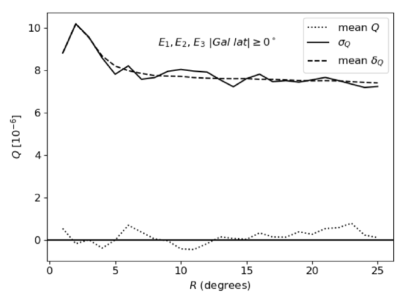
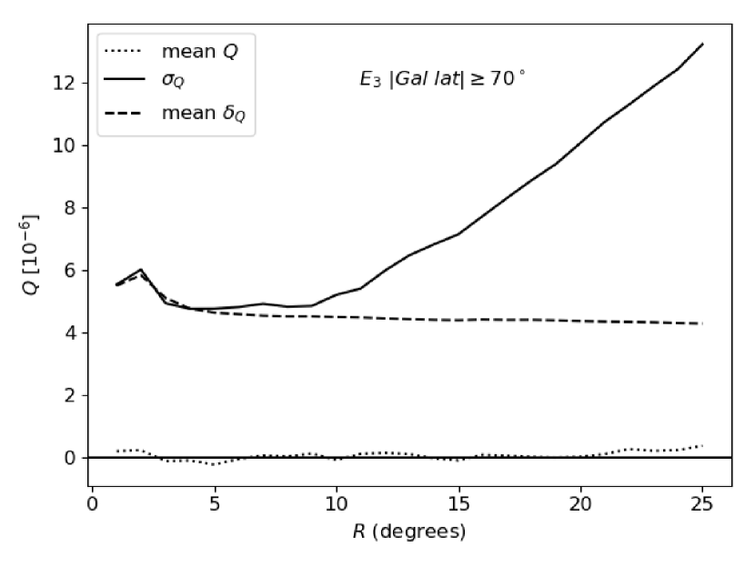
Figure 2.— Summary statistics for the 500 Monte Carlo simulations using a uniform photon arrival direction using no latitude cut (top), a latitude cut of $70^{\circ}$ for all three sets (middle), and a latitude cut of $70^{\circ}$ for $E_{3}$ only (bottom). Shown are for each $R$ the mean value of $Q$ (dotted curve), the mean value of $\delta_{Q}$ (dashed curve), and the standard deviation $\sigma_{Q}$ (solid curve) of the obtained distribution from the simulations. $R$ is the radius of the circle used to select the low energy photons, see the text for details.

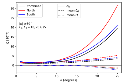
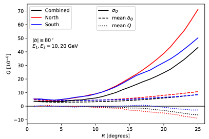
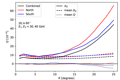
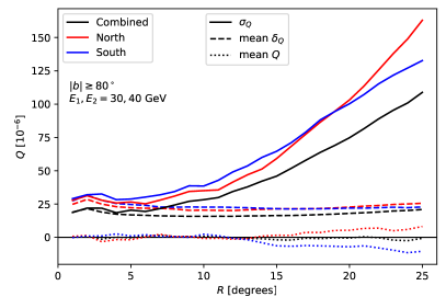
Figure 3.— Summary statistics for the 200 simulations of an isotropic sky accounting for the LAT instrument response and observing profile. The two columns represent different latitude cuts and each row a different energy bin combination. Shown are for each $R$ the mean value of $Q$ (dotted curves), the mean value of $\delta_{Q}$ (dashed curves), and the standard deviation $\sigma_{Q}$ (solid curves) of the obtained distribution from the simulation. Results for the north (red color) and the south (blue color) hemisphere are shown independently, as well as the results from the hemispheres combined (black color).

The simulations of uniform photon arrival directions are performed to test the code implementation and also to test the effect of the latitude cut without introduction of any spatial dependence in the photon distribution on the sphere. Photon arrival directions are sampled uniformly on the sphere by sampling independently in longitude and cosine of colatitude. Three sets were sampled and the number of photons in each sample corresponds roughly to the number of photons selected above $60^{\circ}$ latitude for the 10, 20, and 50 GeV ranges. For these simulations, the number of photons is always the same in each bin, independent of the latitude cut applied. For each latitude cut, 500 simulations are performed, each using a different seed for the pseudo-random number generator. For each simulation, the value of $Q$ is calculated for $R$ from $1^{\circ}$ to $25^{\circ}$ in steps of $1^{\circ}$. For each value of $R$, the mean of the $Q$ values, the mean of the $\delta_{Q}$ values, and the standard deviation of the $Q$ values, $\sigma_{Q}$, are calculated. If everything works as expected, then the value of $\sigma_{Q}$ and the mean of $\delta_{Q}$ should be identical, and the mean value of $Q$ should be zero.

Figure 2 shows the summary statistics for the 500 sets of simulations employing the three different latitude cuts. The mean value of $Q$ for these simulations is consistent with 0 for all latitude cuts and the mean value of $\delta_{Q}$ agrees with $\sigma_{Q}$ when the latitude cut is the same for all photon sets. The only difference between applying a latitude cut and not in that case is the magnitude of the error which increases significantly with $R$ if a latitude cut is applied. With no latitude cut at all a larger patch radius will always include more photons, uniformly distributed around the arrival direction of the selected $E_{3}$ photon. The uncertainty of the $Q$ value thus slightly decreases with increasing $R$. Applying a latitude cut, however, causes both the spread and the value of $\delta_{Q}$ to increase with $R$. This is expected for geometrical reasons; when the same latitude cut is applied for all energy bins, patches near the boundary will not be circular but have a sharp cut off. This means the photons will not be uniformly distributed around $E_{3}$, but concentrated on the higher-latitude side of the direction of the photon leading to a larger value for those items in the sum of Equation (3). This increases $\delta_{Q}$ and the absolute values of $Q$, which in turn increases the standard deviation of the distribution of $Q$ values.

In the case where a latitude cut is applied only to the $E_{3}$ photons, the values of $\delta_{Q}$ and $\sigma_{Q}$ start to deviate for larger values of $R$. While $\delta_{Q}$ follows a trend similar to that when no latitude cut is applied, $\sigma_{Q}$ more closely resembles the results with a latitude cut, although with a smaller magnitude. The onset of the deviation depends on the latitude cut, starting at smaller $R$ for more strict latitude cuts. This indicates that it is a boundary effect, but a concrete reason for this behavior is not understood at the moment. It is, however, clear that $\delta_{Q}$ significantly underestimates the statistical uncertainty of the measurements when a latitude cut is applied only to $E_{3}$. Note though that the statistical uncertainty in this case is still smaller than when applying the latitude cut to all energy bins and this method is therefore still preferred. Hereon, the latitude cut is thus only applied to the photons in the highest energy bins, while for the other bins the photon directions are restricted to being within $D(\mbox{\boldmath$n$}{}_{k},R)$.

3.2. Isotropic Emission

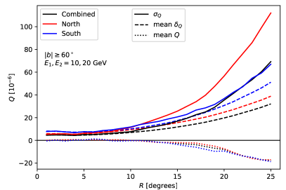
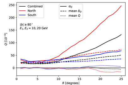
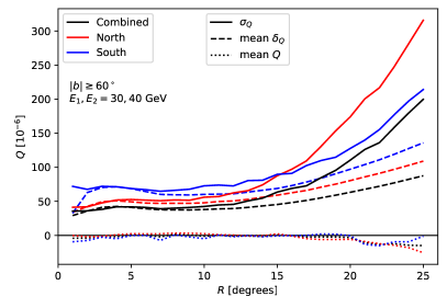
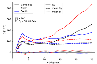
Figure 4.— Summary statistics for the 200 simulations of the interstellar emission accounting for the LAT instrument response and observing profile. The two columns represent different latitude cuts and each row a different energy bin combination. Similar statistics are shown in Figure 3 for the isotropic emission.

The unresolved extragalactic emission at GeV energies is approximately isotropic (e.g., Ackermann et al., 2015). If the effective area of the instrument and its exposure were uniform over the sky, this isotropic emission would lead to a uniform distribution of photon direction. This is, however, not the case and the effect was not studied explicitly by Tashiro et al. (2014). The effective area of the instrument is dependent on both the energy and the incident angle of the photon which, combined with the observing profile of the LAT, leads to a non-uniform distribution of photon directions that is slightly energy dependent. To test the effect of this on the $Q$ statistics, 200 simulations were performed using gtobssim accounting for the true observing profile of the LAT for the same period as the observed data. The input model assumed isotropic emission with a power-law distribution in energy having an index of $-2.3$ that approximately matches the emission given in ‘iso_P8R3_SOURCE_V2_v1.txt’ . Care was taken to assign a unique seed to each simulation and, because the simulations use a realistic emission model, the numbers of photons are similar to the counts in the LAT data.

Figure 3 shows the results from these simulation using similar summary statistics as in Figure 2. The only difference here is that the results are shown separately for the north and the south pole to see if there is any hemispherical difference. In their original work, Tashiro et al. (2014) found the signal to be more significant in the northern hemisphere than in the southern one, so it is important to see if the exposure causes this. Comparison between the results of the uniform photon distribution and the isotropic emission reveals interesting similarities, but also differences. The latitude cut applied to the data results in a similar deviations between $\sigma_{Q}$ and the mean of $\delta_{Q}$, but the effect of the exposure leads to an even larger discrepancy. Also, rather than being constant with increasing $R$, the value of $\delta_{Q}$ rises slightly with $R$. When comparing the results for the two hemispheres separately, it is clear that $\sigma_{Q}$ is consistently larger in the north compared to the south at larger $R$. This is despite the northern hemisphere containing more photons in the simulation than the south. It is not clear whether the non-uniformity of the arrival direction causes these changes, but the conclusion is that simulations are required to get an accurate estimate of the true uncertainty of the measurement of $Q$.

Because the exposure of the LAT is slightly energy dependent in the energy range considered, there is the possibility that it causes a bias in the determination of the value of $Q$. While there seems to be a small deviation from zero and therefore a small bias in the results shown in Figure 3, detailed investigations of the individual simulations show that these are caused by single outliers and the median value is closer to zero. To distinguish between the effects of limited statistics and a proper bias, calculations of the $Q$ values from the binned exposure maps under the assumption of “infinite” statistics were performed by using the pixel locations as photon directions and the pixel values as photon “counts”. This resulted in biases that were orders of magnitude smaller than indicated by the simulations and the value of $Q$ is therefore not biased by the exposure.

3.3. Interstellar Emission

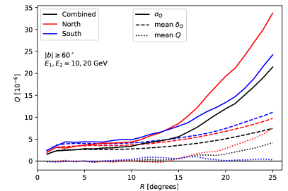
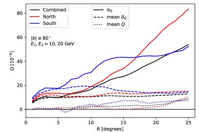
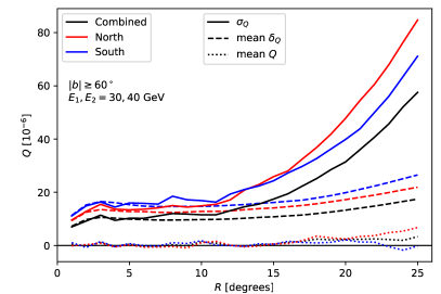
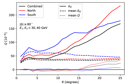
Figure 5.— Summary statistics for the 200 simulations of the combined interstellar and isotropic emission accounting for the LAT instrument response and observing profile. The two columns represent different latitude cuts and each row a different energy bin combination. Similar statistics are shown in Figure 3 for the isotropic emission only and in Figure 4 for the interstellar emission only.

Another important consideration is the interstellar emission. Despite the usage of latitude cuts to reduce its contribution, the interstellar emission is still a large fraction of the total observed emission. Because of its origin in interactions between cosmic rays and the interstellar medium, the interstellar emission is very structured and some of that structure is energy dependent. It has thus the potential to introduce a bias in the $Q$ statistic. To test this, 200 simulations were performed using gtobssim, this time using the interstellar emission model gll_iem_v06.fit as input.

The summary statistics for these simulations are shown in Figure 4 for the same latitude cuts and energy bins as used in Figure 3 for the isotropic simulations. The most noticeable difference is the significantly larger range of $\sigma_{Q}$ compared to the isotropic simulations. This is expected, because the interstellar emission is less intense than the isotropic emission and it also falls off more quickly with energy and latitude, leading to fewer photons for the evaluation of the $Q$ statistic and hence larger statistical errors. For example in the 10 GeV bin, the number of photons is similar in the simulations of the two emission models for the latitude cut of $60^{\circ}$ while with a cut of $80^{\circ}$, the number of photons for the interstellar emission simulation is only half of that using the isotropic emission. Also, the number of photons in the 50 GeV bin in the interstellar emission simulations is always much smaller than that in the same bin in the isotropic simulations, with only about 10 photons in each hemisphere when a latitude cut of $80^{\circ}$ is applied.

Another interesting trend to notice is the dependence of the mean of $\delta_{Q}$ on $R$ for the two different latitude cuts. The looser cut of $60^{\circ}$ results in the values increasing with $R$ while for the $80^{\circ}$ cut, the values are nearly constant and more in line with the results from the isotropic simulations shown in Figure 3. It thus seems that the structure in the interstellar emission increases the uncertainty of the measurement with increasing $R$ and that this increase is dependent on latitude. The latitude dependence is of course expected and is the reason for applying a latitude cut in the first place. Finally, the hemispheric dependence of the uncertainties at large $R$ is striking. In many cases, the southern hemisphere shows smaller uncertainties than the combined emission, meaning that something about the structure of the emission is causing a large scatter in the calculations. This is despite the fact that the combined analysis uses about twice as many photons than that in the southern hemisphere and demonstrates the importance of using these simulations to estimate the uncertainty of the measurements.

There is a hint of a bias in the determination of $Q$ from the interstellar emission model. The mean value of $Q$ from the 200 simulations is clearly offset from 0 at higher values of $R$ for most of the permutations of energy bins and latitude cuts (not all are shown here). The bias is negative in all cases where it can be seen (e.g., the top left panel in Figure 4), which is in contrast to the simulations of the isotropic emission that showed both positive and negative biases. To verify this, a calculation of $Q$ was performed using “infinite” statistics, basically calculating the value of $Q$ based on the pixel values in the input map gll_iem_v06.fit. Those calculations confirmed a small bias in the calculation at the level of $\sim 10^{-6}$. The bias is seen to increase with $R$ and always be negative. It is thus smaller than the statistical uncertainty and the larger indications of biases shown in Figure 4 are a result of statistical fluctuations in the simulations. It should also be emphasized that the bias will be much reduced in the more realistic simulations that include both the interstellar and the isotropic emissions discussed in the next subsection, because the isotropic emission provides the larger fraction of photons.

3.4. Combined Emission

As has been shown in the previous subsections, $\delta_{Q}$ is not a reliable estimator of the statistical uncertainty of the results. To create simulated diffuse emission data as realistic as possible, the simulations of the isotropic and interstellar emission described in the previous subsections are combined one by one. For the proper estimation of the uncertainty of the measurement it is important to have similar numbers of photons in each simulation and the observed data. Even accounting for the effects of the point source mask, the number of photons in the simulations is slightly larger than that in the data. The exact ratio of the two depends on the latitude cut and the energy range, and is different between the two hemispheres. To calculate the ratio, the average numbers of photons in the 202 simulations were compared to the actual number of photons in the data. The ratio varies from being nearly 1 in the northern hemisphere for the 50 GeV bin and the latitude cut of $b>80^{\circ}$ to being 0.65 in the southern hemisphere also at 50 GeV and the latitude cut of $b<-80^{\circ}$. In general, however, the ratio is around 0.95 in the north and 0.9 in the south. This discrepancy is due to the models not accurately representing the data. In particular, the north–south asymmetry is well known and cannot be accounted for by the current interstellar emission models in combination with an isotropic background (Ackermann et al., 2012). To account for this difference, the ratios are used to determine the fractions of photons that are removed from the simulations by random selection. It was found that accounting for this increased the uncertainty estimate by up to 20%, the increase being largest in the south for the tightest latitude cut. The $\sigma_{Q}$ results from these combined simulations are used as the statistical uncertainties of the calculations for the observed LAT data.

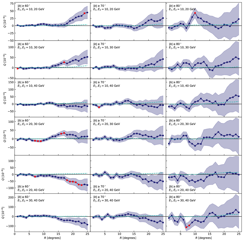
Figure 6.— The value of $Q$ calculated using the LAT data is shown as blue boxes and the shaded region represents the uncertainty of the measurements as estimated from the combined simulations described in Section 3.4. Also plotted is the mean value of $Q$ from the combined simulation as a dashed cyan curve. Points that deviate by more than 2$\sigma_{Q}$ away from the simulation mean are shown red. Each column represent a different latitude cut of $60^{\circ}$, $70^{\circ}$, and $80^{\circ}$ from left to right and each row has a different combination of energy bins as indicated in each panel.

Figure 5 shows the summary statistics for the combined simulations. Not surprisingly, the results are very similar to those for the isotropic emission only (Figure 3) because the isotropic emission is dominant. There are, however, notable differences mostly caused by the reduced statistics because of the source mask. For the latitude cut of $60^{\circ}$ and combinations using $E_{1},E_{2}=10,20$ GeV, the value of $\sigma_{Q}$ is nearly a factor of 2 larger for $R<5^{\circ}$, but the difference is smaller at larger $R$. For the $E_{1},E_{2}=30,40$ GeV combination, the fractional change is similar at small $R$, but at large $R$ the value of $\sigma_{Q}$ is about 25% larger in the combined simulations. This reflects the steeper spectrum of the interstellar emission that is more important at low energies. For the tighter latitude cut of $80^{\circ}$, this effect is not seen and the value of $\sigma_{Q}$ is slightly larger in the combined simulation than it is in the isotropic simulation due to the source mask. The $R$ dependence is also different, in particular for the south where the value of $\sigma_{Q}$ is significantly larger. Comparison of the values of $\sigma_{Q}$ and the mean of $\delta_{Q}$ shows that the latter starts to underestimate the statistical uncertainty for values of $R$ between about $5^{\circ}$ and $10^{\circ}$. The difference is small at first, but rises up to a factor of 2 to 3 at $15^{\circ}$ and to a factor of 3 to 5 at $20^{\circ}$. Without a proper estimate of the uncertainty, the significance of results at large $R$ can thus be significantly overestimated.

The possible bias seen in the results in Figure 5 in the mean of the $Q$ values is a statistical fluctuation in the simulation caused by strong outliers rather than a real effect. The bias is also much smaller than $\sigma_{Q}$. Using the uncertainty of the mean as an estimator for the statistical significance of the bias in the simulations results in it being less than a 2$\sigma$ effect. Given that there are 18 combinations of latitude cuts and energy bins, this could easily be a statistical fluctuation. It may, however, indicate that the distribution of the $Q$ values does not follow the normal distribution and may have more extended tails. Many more simulations are required to study that in detail. As will be shown in the next section, a 1$\sigma$ estimate of the uncertainty is enough at the moment and further exploration of this is deferred to future work.

4. Application to LAT data

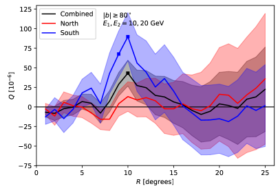
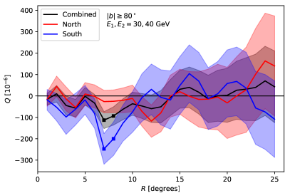
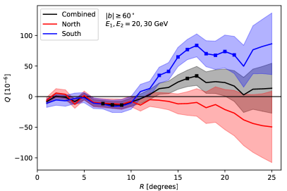
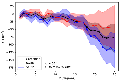
Figure 7.— Examples of the results from calculating $Q$ from the LAT data separately for the northern and southern hemispheres. The shaded regions represent the measurement uncertainties as evaluated from the combined simulations described in Section 3.4. The selected latitude cuts and energy bin combinations all have a 2$\sigma$ outlier in the combined data around $R=7^{\circ}$, see Figure 6. Points that deviate more than 2$\sigma_{Q}$ away from the simulation mean are shown as squares.

The results for the calculation of $Q$ from the observed LAT data are given in Figure 6. It shows all combinations of latitude cuts and energy bins with points that deviate more than 2$\sigma_{Q}$ from the simulation mean shown in red. There is a clear latitude dependence, with the $60^{\circ}$ latitude cut showing in many cases an increasing deviation from 0 with increasing $R$ that is not seen when using only high-energy events above $80^{\circ}$. The sign of the deviation depends on the combination of energy bins and is likely caused by contamination of emission from the Galactic plane and it is within 2 $\sigma_{Q}$ in all but one case where 6 consecutive points are just above the limit. To estimate the significance of this, the fraction of cases with 6 consecutive deviations in the simulations was estimated. This turned out to be around 0.9%, indicating that 0.16 such are expected in our 18 combinations of latitude cuts and energy bins. Measuring one when only 0.16 is expected happens in about 1.2% of the cases, resulting in a statistical significance of a little less than 3 sigma. Apart from this deviation, only 13 other points are shown in red, of which there is a single triplet and two pairs. The simulations were again used to estimate the fractions of such pairs and the expected number is 0.7 for triplets, 1.6 for pairs, and 6 for single points. These 13 points are therefore statistically consistent with noise.

The large reduction in significance compared to the results of Tashiro et al. (2014) is caused by the much improved estimate of the statistical significance through realistic simulations with gtobssim. Using only $\delta_{Q}$ as the uncertainty would lead to a significant signal in many of the calculations shown here, but without a clear trend in handedness. The most significant signal seen by Tashiro et al. (2014) was for $E_{1},E_{2}=10,40$ GeV and a latitude cut of $80^{\circ}$, which shows no sign of signal in the present analysis, even when using $\delta_{Q}$ as the error estimator. Their results also indicated that the signal peaked at around $R=12^{\circ}$, something that is not seen in Figure 6. In contrast, the few significant points at $R=7^{\circ}$ are not visible in Figure 3 of Tashiro et al. (2014). Their results are thus likely caused by statistical fluctuations and were overstated because of underestimated uncertainties. This was already hinted at in the analysis of Chen et al. (2015), where the inclusion of the LAT exposure in the simulations reduced the significance of the signal.

As a check, the data was analyzed separately in the northern and southern hemispheres. Splitting the data into twice as many bins does result in more 2$\sigma$ outliers. Most notably though, the number of outliers in the northern hemisphere is smaller than expected from the simulations while those in the southern hemisphere are more numerous than expected. This is mostly caused by many consecutive points being slightly above the 2$\sigma_{Q}$ limit at large values of $R$ for the latitude cuts of $-60^{\circ}$ and $-70^{\circ}$. For the former, 5 out of 6 have these deviations while 3 out of 6 show deviation for the latter. No such deviations are seen at the tightest latitude cut of $-80^{\circ}$. The deviations are both positive and negative and in some cases the northern hemisphere shows indication of a small signal with the opposite sign to that of the southern one. The outliers also show a steady rise with $R$ and do not portray any visible structure. Having so many outliers is statistically unlikely and more simulations are needed to accurately estimate the statistical significance. This putative signal is though unlikely to originate from extragalactic processes, because it is only seen for one of the hemispheres and only for loose cuts in Galactic latitude. A small selection of the results is shown in Figure 7 focusing on the few bins with significant outliers in the combined data. Examination of the hemispheric dependence further illustrates that the few outliers visible in the combined data are likely statistical outliers. In two cases, the signal is caused by a spike in the southern hemisphere that is not present in the north while in the other two it is a fluctuation in both hemisphere. Examination of the hemispheric dependence reveals that there is very little correlation between the two hemispheres, and the largest deviation from 0 in the combined signal occurs when the signals happen to deviate in the same direction. There is, however, no clear trend in the structure of the signal either when looking at different latitude cuts or different energy bins. The marginally significant results are thus likely caused by statistical fluctuations.

A possible explanation for the missing signal is the usage of the P8R3 SOURCE data compared to the Pass 7 CLEAN data used in Tashiro et al. (2014). While it is difficult to compare the classes directly, the P8R3 Source data is expected to have a slightly higher background rate than the Pass 7 Clean data. To test the effect of this, the calculations of the $Q$ values were repeated with the much cleaner P8R3 ULTRACLEANVETO data. The results are qualitatively similar to those already presented, but due to the lower acceptance, the statistical power of the analysis is reduced. The results are therefore compatible with being statistical fluctuations and the lack of signal is thus not caused by background contamination in the SOURCE event class.

Another difference between the current analysis and those of Tashiro et al. (2014) and Chen et al. (2015) is the use of the 4FGL catalog cutting out a $2^{\circ}$ diameter around the sources instead of the LAT first high-energy source (1FHL) catalog (Ackermann et al., 2013) with a cut of $3^{\circ}$ diameter. Using the 1FHL catalog would be inappropriate with the larger dataset, but to test the effect of this, the analysis was repeated using the LAT third high-energy source (3FHL) catalog (Ajello et al., 2017) and the larger cut. The 3FHL is the most recent in the series of high-energy catalogs, using photons with energies between 10 GeV and 2 TeV for source detection. It is therefore appropriate for analysis in this energy range. The results are qualitatively consistent with the current results and the point source cut does not affect the main conclusions of this work.

5. Conclusions

The work of Tashiro et al. (2014) looking for handedness in the arrival directions of Fermi-LAT photon data has been repeated with improved LAT event reconstruction and more data. Several Monte Carlo simulations were performed to accurately estimate the uncertainty of the results. The new error estimate, $\sigma_{Q}$, is often significantly larger than $\delta_{Q}$, the error estimate used in Tashiro et al. (2014), resulting in no clear signal of handedness. As demonstrated here, $\sigma_{Q}$ better reflects the true spread in the $Q$ values. It also reveals unexpected boundary effects due to the latitude cuts, which need further investigation.

There is a hint of a nearly 3$\sigma$ signal at large radii for $E_{1},E_{2}=20,40$ GeV and a latitude cut of $60^{\circ}$, but the signal is absent for the tighter latitude cuts and is therefore likely caused by contamination from Galactic emission. A similar feature is visible in the results of Tashiro et al. (2014) for the same energy bin, but the signal also decreases significantly with more stringent cuts on latitude. The most promising data selection in Tashiro et al. (2014) using $E_{1},E_{2}=10,40$ GeV and a latitude cut of $80^{\circ}$, showed in their analysis a signal of left handedness with an estimated significance of about $3\sigma$ but is, in the current analysis, compatible with 0 and not even a slight hint of a signal at $R=12^{\circ}$.

This conclusion does not rule out the existence of a helical cosmological magnetic field. Several assumptions are made in the physical motivation presented by Tashiro et al. (2014). For instance, there is no way of knowing how many of the photon triples used actually do originate from the same source. It may very well be so that there are so few that any signal they might carry is completely drowned by the background. In other words, the constructed $Q$ statistic in Equation (3) may in practice not be as closely related to the helical part of the correlator of the magnetic field as assumed. In fact, Duplessis & Vachaspati (2017) show that random fluctuations in the magnetic field can induce spurious signals in the $Q$ statistic and averaging over many realizations is needed to accurately trace the observed signal back to the helicity of the magnetic field; even the sign may be incorrectly estimated. They propose a modification to the $Q$ statistic that can improve the power to determine the handedness, but it is unclear if the improvements can overcome the effects of the unknown structure of the magnetic field.

We emphasize that our main objective was to see whether—independently of any model or physical assumptions—there exists any handedness in the LAT data. In view of our new findings concerning the relatively large error bars, our answer to this question is no. This does not necessarily imply that any intergalactic magnetic field must be weak or that the method of Tashiro & Vachaspati (2013) is not sensitive enough. It is possible that specific selection methods in time or shape of the photon triplets could yield a significant result for $Q$. As discussed in this paper, it is possible that a finite value of $Q$ could be caused by regions of different sizes and different energy ranges in which photons accumulate to a density that is higher than the average. This could either be caused by instrumental effects (for example by a nonuniformity of exposure) or it could be caused by a handedness of processes within our Galaxy. A possible candidate could be the Galactic magnetic field. In such a case, the causal connection with $Q$ would be different from what was anticipated by Tashiro & Vachaspati (2013). However, given that there is currently very little evidence for any handedness, neither globally or locally for the northern or southern Galactic hemispheres these possibilities remain just speculation.

References

- Ackermann et al. (2015) Ackermann, M. et al. 2015, ApJ, 799, 86, 1410.3696
- Ackermann et al. (2013) ——. 2013, ApJS, 209, 34, 1306.6772
- Ackermann et al. (2012) ——. 2012, ApJ, 750, 3, 1202.4039
- Ajello et al. (2017) Ajello, M. et al. 2017, ApJS, 232, 18, 1702.00664
- Asplund (2019) Asplund, J. 2019, No sign of a left-handedness in GeV photon arrival directions (Bachelor’s thesis, Stockholm Univ., http://su.diva-portal.org)
- Atwood et al. (2009) Atwood, W. B. et al. 2009, ApJ, 697, 1071, 0902.1089
- Batista et al. (2019) Batista, R. A., Saveliev, A., & de Gouveia Dal Pino, E. M. 2019, MNRAS, 2062, 1904.13345
- Berger & Field (1984) Berger, M. A., & Field, G. B. 1984, Journal of Fluid Mechanics, 147, 133
- Bourdin & Brandenburg (2018) Bourdin, P.-A., & Brandenburg, A. 2018, ApJ, 869, 3, 1804.04160
- Boyarsky et al. (2012) Boyarsky, A., Fröhlich, J., & Ruchayskiy, O. 2012, Phys. Rev. Lett., 108, 031301
- Brandenburg et al. (2017a) Brandenburg, A., Kahniashvili, T., Mandal, S., Pol, A. R., Tevzadze, A. G., & Vachaspati, T. 2017a, Phys. Rev. D, 96, 123528, 1711.03804
- Brandenburg et al. (2017b) Brandenburg, A., Schober, J., Rogachevskii, I., Kahniashvili, T., Boyarsky, A., Fröhlich, J., Ruchayskiy, O., & Kleeorin, N. 2017b, ApJL, 845, L21
- Broderick et al. (2018) Broderick, A. E., Tiede, P., Chang, P., Lamberts, A., Pfrommer, C., Puchwein, E., Shalaby, M., & Werhahn, M. 2018, ApJ, 868, 87, 1808.02959
- Bruel et al. (2018) Bruel, P., Burnett, T. H., Digel, S. W., Johannesson, G., Omodei, N., & Wood, M. 2018, arXiv e-prints, arXiv:1810.11394, 1810.11394
- Chen et al. (2015) Chen, W., Chowdhury, B. D., Ferrer, F., Tashiro, H., & Vachaspati, T. 2015, MNRAS, 450, 3371, 1412.3171
- Díaz-Gil et al. (2008a) Díaz-Gil, A., García-Bellido, J., García Pérez, M., & González-Arroyo, A. 2008a, Physical Review Letters, 100, 241301, 0712.4263
- Díaz-Gil et al. (2008b) ——. 2008b, Journal of High Energy Physics, 7, 043, 0805.4159
- Duplessis & Vachaspati (2017) Duplessis, F., & Vachaspati, T. 2017, J. Cosmology Astropart. Phys, 2017, 005, 1701.01501
- Frauenfelder et al. (1957) Frauenfelder, H., Bobone, R., von Goeler, E., Levine, N., Lewis, H. R., Peacock, R. N., Rossi, A., & de Pasquali, G. 1957, Physical Review, 106, 386
- García-Bellido et al. (2004) García-Bellido, J., García Pérez, M., & González-Arroyo, A. 2004, Phys. Rev. D, 69, 023504, hep-ph/0304285
- García-Bellido et al. (1999) García-Bellido, J., Grigoriev, D., Kusenko, A., & Shaposhnikov, M. 1999, Phys. Rev. D, 60, 123504, hep-ph/9902449
- Joyce & Shaposhnikov (1997) Joyce, M., & Shaposhnikov, M. 1997, Phys. Rev. Lett., 79, 1193
- Kahniashvili et al. (2005) Kahniashvili, T., Gogoberidze, G., & Ratra, B. 2005, Physical Review Letters, 95, 151301, astro-ph/0505628
- Kahniashvili & Ratra (2005) Kahniashvili, T., & Ratra, B. 2005, Phys. Rev. D, 71, 103006, astro-ph/0503709
- Lee & Yang (1956) Lee, T. D., & Yang, C. N. 1956, Physical Review, 104, 254
- Moffatt (1978) Moffatt, H. K. 1978, Magnetic field generation in electrically conducting fluids (Cambridge, England, Cambridge University Press)
- Neronov & Vovk (2010) Neronov, A., & Vovk, I. 2010, Science, 328, 73
- Rothery et al. (2011) Rothery, D. A., Gilmour, I., & Sephton, M. A. 2011, An Introduction to Astrobiology (Cambridge, UK: Cambridge University Press)
- Tashiro et al. (2014) Tashiro, H., Chen, W., Ferrer, F., & Vachaspati, T. 2014, MNRAS, 445, L41, 1310.4826
- Tashiro & Vachaspati (2013) Tashiro, H., & Vachaspati, T. 2013, Phys. Rev. D, 87, 123527, 1305.0181
- Tashiro et al. (2012) Tashiro, H., Vachaspati, T., & Vilenkin, A. 2012, Phys. Rev. D, 86, 105033
- The Fermi-LAT collaboration (2019) The Fermi-LAT collaboration. 2019, arXiv e-prints, arXiv:1902.10045, 1902.10045
- Vachaspati (1991) Vachaspati, T. 1991, Physics Letters B, 265, 258
- Vachaspati (2001) ——. 2001, Phys. Rev. Lett., 87, 251302