Robust Stackelberg controllability for the Kuramoto–Sivashinsky Equation

Abstract.

In this article the robust Stackelberg controllability (RSC) problem is studied for a nonlinear fourth–order parabolic equation, namely, the Kuramoto–Sivashinsky equation. When three external sources are acting into the system, the RSC problem consists essentially in combining two subproblems: the first one is a saddle point problem among two sources. Such an sources are called the “follower control” and its associated “disturbance signal”. This procedure corresponds to a robust control problem. The second one is a hierarchic control problem (Stackelberg strategy), which involves the third force, so–called leader control. The RSC problem establishes a simultaneous game for these forces in the sense that, the leader control has as objective to verify a controllability property, while the follower control and perturbation solve a robust control problem. In this paper the leader control obeys to the exact controllability to the trajectories. Additionally, iterative algorithms to approximate the robust control problem as well as the robust Stackelberg strategy for the nonlinear Kuramoto–Sivashinsky equation are developed and implemented.

1. Main problems. Robust Stackelberg controllability

The Stackelberg strategy is a concept from game theory which appears with the publication by Heinrich Von Stackelberg in 1934 “ Market structure and equilibrium”. It is a non–cooperative competition game with applications to economic processes that involves two–player with a hierarchic structure, namely, the first player (called the leader) enforce its strategy on the other player, and then the second player (called the follower) reacts trying to win or optimize the answer to the leader movement, see [38, 40]. The previous sentences correspond to a general notion on a Stackelberg strategy, which is applied in the context of hierarchic control for some models described by partial differential equations (PDEs).

On the other hand, the robustness in a control system is the sensitivity to the effects that are not considered in the analysis and design such as disturbance signals and noise measurements. In other words, a system is said to be robust when it is hardy, durable and resilient, and also stable over the range of parameter variations. In this sense, one could think in the worst–case disturbance of the system, and design a controller which is suited to handle even this extreme situation. Thus, the problem of finding a robust control involves the problem of finding the worst-case disturbance in the spirit of a non–cooperative game (when there is no cooperation between the controller and disturbance function), that means from a mathematical point of view to reach a saddle point for the pair disturbance–controller. In the literature there are many works concerning robust control problems, see for instance the books [18, 14, 12, 10] and its references therein for a complete description on this subject.

From a theoretical perspective, recent works have mixed the concept of robust control with a Stackelberg strategy, and applied it to semilinear and linear heat equations [20, 21], and to the Navier–Stokes system [32]. This new idea in control theory is being abridged and called “Robust Stackelberg controllability” (RSC), see Problem 3 below. In the case of a semilinear heat equation [20], the RSC problem used external forces acting into the system, where the leader control has as constrain the controllability to trajectories. On the other hand, [21] solves a RSC problem for the linear heat equation by considering that the either the leader or follower control acts on a small part of the boundary. In [21] the leader control satisfies the null controllability property. In the RSC problem for the Navier–Stokes system [32] all controls are external forces acting on the systems, the leader control has a local null controllability objective, while the perturbation and the follower control solve a robust control problem. However, these three works have three things in common: 1) they deal with systems whose main operator is a second–order operator (Laplace operator, Stokes operator), 2) independent of the configuration or localization of forces (either interior or bounded), the property of the exact controllability to the trajectories for the leader control remains open for nonlinear systems, and 3) as it can see, they do not present any numerical framework.

In what follows we describe the main contributions of this work.

1. We solve the robust internal control problem for the nonlinear KS equation posed on a bonded domain. Our approach use central ideas from robust boundary control problem for the same equation [22]. To do that, several points related to regularity of solutions and to the existence of a saddle point are modified and adapted.

   In the numerical context, to our knowledge, this paper contains the first numerical description concerning the robustness process for the KS equation. Due to the high–order in space (i.e., fourth–order derivates), an appropriate change of variable will be used to implement low–order finite elements, more precisely, $\mathbb{P}_{1}$–type Lagrange elements, meanwhile, a $\theta$–scheme/Adams–Bashforth method is created for the time discretization. Thus, our method does not require a higher–order approach to the KS equation. Although this paper does not present an exhaustive numerical analysis of our method, since it is far way of the main goals, several configurations to the time–space discretization display good results for the error (among the exact and numeric solution) in the $L^{2}$–norm and $L^{\infty}$–norm. Besides, from the algorithms presented in [6, 39] for the Navier–Stokes system, we propose new iterative schemes of constructing the ascent and descent directions, and whose basis is the preconditioned nonlinear gradient conjugate method.

2. Once we have obtained the robust pair, the robust stackelberg controllability (RSC) problem for the KS equation is studied. The second theoretical contribution of our article is that, as far as we know, we use for the first time the exact controllability to the trajectories for the leader control subject to a nonlinear system. The main novelties are new Carleman inequalities and its relationship with the robustness parameters. Additionally, since the leader control obeys to the exact controllability to the trajectories and its formulation includes a coupled system of fourth–order equations, new algorithms based in regularization techniques are introduced and implemented. Finally, we want to highlight the sensitivity in the robustness parameters, the initial data, and also on the different subdomains for obtaining good results. Indeed, numerical experiments show that non–cooperative relation among the leader control and follower might be removed in some sense.

1.1. Main problems

In an abstract setting, the main problems to treat can be formulated as follows: let $(X,\langle\cdot,\cdot\rangle)$ be an Hilbert space and let $(\mathcal{A},D(\mathcal{A}))$ be an unbounded operator in $X$ such that $-\mathcal{A}$ generates an analytic semigroup in $X$. Let $(U,[\cdot,\cdot])$ be another Hilbert space and for $i=1,2$,  let $\mathcal{B}_{i}$ be bounded operators from $U$ into $D(\mathcal{A}^{*})^{\prime}$. Moreover, let $\Omega$ be a nonempty bounded connected open subset of $\mathbb{R}^{d}$ of class $C^{\infty}$, $d\in\mathbb{N}$, and let $\omega$ be a (small) nonempty open subset of $\Omega$. Let $T>0$ be given. We use the notation $Q:=\Omega\times(0,T)$,  $\Sigma:=\partial\Omega\times(0,T)$.

Let us consider the non–homogeneous evolution problem

$$\left\{\begin{array}[]{lll}\begin{array}[]{llll}u_{t}+\mathcal{A}u+\mathcal{N}u=h1_{\omega}+\mathcal{B}_{1}v+\mathcal{B}_{2}\psi&\text{ in }&Q,\\ u(\cdot,0)=u_{0}(\cdot)&\text{ in }&\Omega,\end{array}\end{array}\right.$$ (1.1)

where $\mathcal{N}$ is associated to the nonlinear part, and the functions $h,v,\,\psi$ belong to appropriate spaces. Here, $1_{\omega}$ is the characteristic function of the set $\omega$. In (1.1) the interior forcing has been decomposed into a function $\psi$, called disturbance signal, and two functions, $h$ and $v$. In our framework $h=h(x,t)$ will be called the “leader control”, meanwhile $v=v(x,t)$ will be called the “follower control”. To be precise, the interaction between such functions and the problems that arise from them as well as the operators $\mathcal{B}_{1},\,\mathcal{B}_{2}$ will be defined below for every problem. In this abstract framework, the cost functional is given by

$$J_{r}(v,\psi;h):=\frac{1}{2}\iint\limits_{\mathcal{O}_{d}\times(0,T)}|u-u_{d}|^{2}dxdt+\frac{1}{2}\Biggl{(}\ell^{2}\int\limits_{0}^{T}\|\mathcal{B}_{1}v\|_{X}^{2}dt-\gamma^{2}\int\limits_{0}^{T}\|\mathcal{B}_{2}\psi\|_{Y}^{2}dt\Biggr{)},$$ (1.2)

where $X,Y$ are suitable Sobolev spaces, $\mathcal{O}_{d}$ is a nonempty open subset of $\Omega$,  $u_{d}$ is a given function and $\ell,\gamma$ are positive constants. The parameter $\ell$ can be interpreted as a measure of the “cost” of the control to the engineer. Thus, when $\ell\to+\infty$, it corresponds to the “expensive” control, and results in $v\to 0$ in the minimization with respect to $v$ for the present problem. On the other hand, reduced values of $\ell$, corresponding to cheap control, reduce the increase in the cost functional upon the application of a control $v$. Similarly, the parameter $\gamma$ can be interpreted as a measure of the price of the disturbance. The limit as $\gamma\to+\infty$ results in $\psi\to 0$ in the maximization with respect to $\psi$, and reduced values of $\gamma$ decrease the cost functional upon the application of a disturbance $\psi$.

Problem 1.

Robust control. In (1.1), $h\equiv 0$ and $\mathcal{B}_{1},\,\mathcal{B}_{2}$ are mapping from $L^{2}(\Omega)$ into itself. The robust internal control problem consists in finding a unique pair $(\overline{v},\overline{\psi})\in L^{2}(Q)^{2}$ such that

$$J_{r}(\overline{v},\psi;0)\leq J_{r}(\overline{v},\overline{\psi};0)\leq J_{r}(v,\overline{\psi};0),\quad\forall(v,\psi)\in L^{2}(Q)^{2},$$ (1.3)

subject to the system (1.1).

Before mentioning the other two problems that we deal in this paper, let $\overline{u}$ be a solution of the homogeneous equation:

$$\begin{cases}\overline{u}_{t}+\mathcal{A}\overline{u}+\mathcal{N}\overline{u}=0&\text{in }Q,\\ \overline{u}(\cdot,0)=\overline{u}_{0}&\text{in }\Omega.\end{cases}$$ (1.4)

Problem 2.

Stackelberg strategy. In (1.1), $\mathcal{B}_{2}\equiv 0$ and $\mathcal{B}_{1}=1_{\mathcal{O}}$, where $\mathcal{O}$ is a small open subset of $\Omega$ with $\mathcal{O}\cap\omega=\emptyset$. The hierarchic control problem consists in finding a leader control $h\in L^{2}(0,T;L^{2}(\omega))$ and a unique follower control $v\in L^{2}(0,T;L^{2}(\mathcal{O}))$ minimizing (1.2), and an associated solution $u$ to (1.1) verifying $u(\cdot,T)=\overline{u}(\cdot,T)$ in $\Omega$, where $\overline{u}$ is solution of (1.4).

Problem 3.

Robust Stackelberg controllability. For every fixed leader control $h$, solve the saddle point problem for the system (1.1), that is, to find the best control $v$ in the presence of the disturbance $\psi$ which maximally spoils the follower control for the system (1.1). Once the saddle point has been identified for each leader control $h$, we deal with the problem of finding the control $h$ of minimal norm satisfying constraints of exact controllability to the trajectories. More precisely, we look for a control $\overline{h}$ such that

$$J(\overline{h})=\min\limits_{h}\frac{1}{2}\iint\limits_{\omega\times(0,T)}|h|^{2}dxdt,\quad\mbox{subject to the restriction}\quad u(\cdot,T)=\overline{u}(\cdot,T)\,\,\,\mbox{in}\,\,\Omega.$$ (1.5)

Remark 1.1.

Note that Problem 2 is a particular case of Problem 3 by considering $\psi=0$ in (1.2). Thus, a Stackelberg strategy is a direct consequence of the robust Stackelberg controllability, and therefore, in this article we will only treat Problem 1 and Problem 3.

1.2. Main results

A particular case of (1.1) corresponds to the Kuramoto–Sivashinsky (KS) equation, it is a fourth-order parabolic equation that serves as a model for phase turbulence in reaction-diffusion systems [24, 25] and also for modeling the diffusive instabilities in a laminar flame [37, 29, 33, 42]. This equation obeys to an one dimensional model, which for our propose is given by

$$\begin{cases}u_{t}+u_{xxxx}+u_{xx}+uu_{x}=h1_{\omega}+v1_{\mathcal{O}}+\psi&\text{in }(0,1)\times(0,T)=:Q,\\ u(0,t)=u(1,t)=u_{x}(0,t)=u_{x}(1,t)=0&\text{on }(0,T),\\ u(\cdot,0)=u_{0}(\cdot)&\text{in }(0,1),\end{cases}$$ (1.6)

where $\omega$ and $\mathcal{O}$ are nonempty open subsets of $(0,1)$ such that $\omega\cap\mathcal{O}=\emptyset$.

From a physical point of view, the term $u_{xx}$ is responsible for an instability at large scales; the dissipative term $u_{xxxx}$ provides damping at small scales; and the non–linear term $uu_{x}$ (which has the same form as that in the Burgers equation) stabilizes by transferring energy between large and small scales. As mentioned, the terms on the right–hand side of (1.6) are representing the leader control, the follower control and the disturbance signal, respectively.

To our knowledge there is no results on robust internal control problem for the KS system (1.6). Thus, our paper fills this gap by using the functional (1.2) with $\mathcal{B}_{1}=1_{\mathcal{O}}$ into $L^{2}((0,1))$ and $\mathcal{B}_{2}=I$ onto $L^{2}((0,1))$. More precisely, the Problem 1 is proved throughout the functional

$$J_{r}(v,\psi;h):=\frac{1}{2}\iint\limits_{\mathcal{O}_{d}\times(0,T)}|u-u_{d}|^{2}dxdt+\frac{1}{2}\Biggl{(}\ell^{2}\iint\limits_{\mathcal{O}\times(0,T)}|v|^{2}dxdt-\gamma^{2}\iint\limits_{Q}|\psi|^{2}dxdt\Biggr{)}.$$ (1.7)

In the context of the robust control, the works [23] and [22] proven robust boundary control problems for the KS equation. In these articles the cost functional is clearly different to the presented for us in (1.2). On the other hand, the techniques of spatially dependent scaling and static output feedback control are used in [35] and [27] for obtaining a robust controller design and an optimal sensor placement for the KS equation, respectively.

Our first main result concerns the robust internal control problem for the KS equation. This is given in the following theorem.

Theorem 1.1.

Let $u_{0}\in H_{0}^{2}(0,1)$ and $h\in L^{2}(0,T;L^{2}(\omega))$ be fixed. Then, for $\gamma$ and $\ell$ sufficiently large, there exists a unique saddle point $(\bar{v},\bar{\psi})\in L^{2}(0,T;L^{2}(\mathcal{O}))\times L^{2}(Q)$ and $u=u(h,\bar{\psi},\bar{v})$ solution of (1.6) such that

$$J_{r}(\psi,\overline{v};h)\leq J_{r}(\overline{v},\overline{\psi};h)\leq J_{r}(v,\overline{\psi};h),\quad\forall(v,\psi)\in L^{2}(0,T;L^{2}(\mathcal{O}))\times L^{2}(Q).$$

As mentioned, the second problem we aim to solve is to find the minimal norm control satisfying a controllability to trajectories constrain. More precisely, let us fix a uncontrolled trajectory of system (1.6), namely, a sufficiently regular solution to

$$\begin{cases}\overline{u}_{t}+\overline{u}_{xxxx}+\overline{u}_{xx}+\overline{u}\overline{u}_{x}=0&\text{in }Q,\\ \overline{u}(0,t)=\overline{u}(1,t)=\overline{u}_{x}(0,t)=\overline{u}_{x}(1,t)=0&\text{on }(0,T),\\ \overline{u}(\cdot,0)=\overline{u}_{0}&\text{in }(0,1).\end{cases}$$ (1.8)

Thus, according to Problem 3, we look for a control $\overline{h}\in L^{2}(0,T;L^{2}(\omega))$ satisfying (1.5).

In the case where $v=\psi=0$, system (1.6) is controllable to trajectories [8]. Recently, for the case where the disturbance disappears, that is, in (1.7) $\psi\equiv 0$, it is possible to deduce that the system (1.6) satisfies a Stackelberg strategy to trajectories [7]. In contrast to [7], this paper shows a different role among the forces $h,v$ and $\psi$ in system (1.6), and therefore, other optimization problems are carried out. In other works, this paper can be seen as an alternative development based in other Carleman estimates for solving Problem 2. Actually, in our framework, the theoretical solution to Problem 2 is a consequence of the simultaneous robust control and hierarchic control, see below Theorem 1.2.

In order to present our second main result, let us define

$$\mathcal{Z}:=C([0,T];H_{0}^{2}(0,1))\cap L^{2}(0,T;H^{4}(0,1))\cap L^{\infty}(0,T;W^{1,\infty}(0,1)).$$ (1.9)

Theorem 1.2.

Assume that $\overline{u}\in\mathcal{Z}$ is the solution of (1.4) and $\omega\cap\mathcal{O}_{d}\neq\emptyset$. Then, for every $T>0$ and $\mathcal{O}\subset(0,1)$ open subset such that $\mathcal{O}\cap\omega=\emptyset$, there exist $\gamma_{0},\ell_{0},\delta>0$ and a positive function $\rho=\rho(t)$ blowing up $t=T$ such that, for any $\gamma\geq\gamma_{0},\,\ell\geq\ell_{0},\,u_{0}\in L^{2}(0,1)$ and $u_{d}\in L^{2}(0,T;L^{2}(\mathcal{O}_{d}))$ satisfying

$$\|u_{0}-\overline{u}_{0}\|_{L^{2}(0,1)}+\displaystyle\iint\limits_{\mathcal{O}_{d}\times(0,T)}\rho^{2}(t)|\overline{u}-u_{d}|^{2}dxdt\leq\delta,$$ (1.10)

there exist a leader control $h\in L^{2}(0,T;L^{2}(\omega))$ and a unique saddle point $(\overline{v},\overline{\psi})\in L^{2}(0,T;L^{2}(\mathcal{O}))\times L^{2}(Q)$ for the functional given by (1.7), and an associated solution $u$ to (1.6) verifying $u(\cdot,T)=\overline{u}(\cdot,T)\mbox{ in }\,(0,1).$

It is worth mentioning again that the theoretical results known up to now on robust Stackelberg controllability (Problem 3) are [20], [32] and [21], and there is no evidence on both numerical algorithms and a controllability to trajectories constrain for the leader control for nonlinear systems. Therefore, this paper we pretend to show theoretical results and carry out numerical schemes jointly with its implementation to Problems 1,3 for the KS equation (1.6).

The rest of the paper is divided as follows: Section 2 contains all theoretical and numerical answers to the robust control problem (see Problem 1) for the system (1.6). First, we present the existence, uniqueness and characterization of the robust control throughout optimal control tools. Afterwards, a discrete scheme for the KS equation (1.6) as well as the procedure to the robust internal control problem are presented. We devote Section 3 to prove the robust Stackelberg strategy for the KS equation, see Theorem 1.2. That means, we prove the exact controllability to the trajectories for the coupled KS system that arises as characterization of the robust control problem. In the theoretical framework, the main tools will be new Carleman estimates and fixed point arguments for coupled fourth–order parabolic systems. Meanwhile, the implemented numerical scheme in the previous section will be adapted and complemented for coupled and discretized KS equations.

2. The robust control problem

The main objetive in robust interior control is to determine the best control function $v\in L^{2}(0,T;L^{2}(\mathcal{O}))$ in the presence of the disturbance $\psi\in L^{2}(Q)$ which maximally spoils the control. In this section we prove the existence, uniqueness and characterization of a solution to the robust internal control problem established in Problem 1 and Theorem 1.1. In what follows, we assume that the leader $h$ has made a choice, so will keep it fixed along this section.

2.1. Existence of the saddle point

This subsection is devoted to solve the minimization problem concerning the robust control problem. First, we prove the existence of a saddle point for the functional defined in (1.7). The proof of existence of a saddle point $(\bar{v},\bar{\psi})$ (Problem 1) is based on the following proposition. Its proof can be found in [15].

Proposition 2.1.

Let $J$ be a functional defined on $X\times Y$ , where $X$ and $Y$ are convex, closed, non–empty, unbounded sets. If

1. $\forall v\in X,\,\psi\longmapsto J(v,\psi)$ is concave and upper semicontinuous.

2. $\forall\psi\in Y,\,v\longmapsto J(v,\psi)$ is convex and lower semicontinuous.

Then the functional $J$ possesses at least one saddle point $(\bar{v},\bar{\psi})$ on $X\times Y$ and

$$J(\bar{v},\bar{\psi})=\min_{v\in X}\sup_{\psi\in Y}\,J({v},{\psi})=\max_{\psi\in Y}\inf_{v\in X}\,J({v},{\psi}).$$ (2.1)

Moreover, if $J$ is strictly concave with respect to $\psi$ and strictly convex with respect to $v$, $(\bar{v},\bar{\psi})$ is unique.

In order to guarantee the existence of the saddle point $(\bar{v},\bar{\psi})$, we prove the following lemma.

Lemma 2.2.

Let $u_{0}\in H_{0}^{2}(0,1)$ be given. Then, there exists positive constants $\gamma_{0}$ and $\ell_{0}$ such that, for any $\gamma\geq\gamma_{0}$ and $\ell\geq\ell_{0}$ we have

1. $\forall v\in L^{2}(0,T;L^{2}(\mathcal{O})),\,\psi\longmapsto J_{r}(v,\psi)$ is concave and upper semicontinuous.

2. $\forall\psi\in L^{2}(Q),\,v\longmapsto J_{r}(v,\psi)$ is convex and lower semicontinuous.

Proof of Lemma 2.2.

First, since the norm is continuous, we only need to check the continuity of the first term in $J_{r}$ with respect to $v,\psi$. To do this, let $u^{i}=u^{i}(v^{i},\psi^{i})\in C([0,T];H_{0}^{2}(0,1))\cap L^{2}(0,T;H^{4}(0,1))$, $i=1,2$ be the solutions of equation (1.6) associated with the corresponding external sources in $L^{2}(Q)$ (see Lemma 5.6 and remark 5.8). Let $\delta u=u^{1}-u^{2}$, $\delta v=v^{1}-v^{2}$ and $\delta\psi=\psi^{1}-\psi^{2}$. Using (1.6), it is easy to verify that $\delta u$ satisfies the following system

$$\begin{cases}(\delta u)_{t}+(\delta u)_{xxxx}+(\delta u)_{xx}+u^{1}(\delta u)_{x}+u^{2}_{x}(\delta u)=\delta v+\delta\psi&\text{in }(0,1)\times(0,T)=:Q,\\ (\delta u)(0,t)=(\delta u)(1,t)=(\delta u)_{x}(0,t)=(\delta u)_{x}(1,t)=0&\text{on }(0,T),\\ (\delta u)(\cdot,0)=0&\text{in }(0,1).\end{cases}$$ (2.2)

Due to the $u^{1},u^{2}_{x}\in L^{\infty}(Q)$, lemma 5.4 allows us to guarantee the existence of a positive constant $C$ depending on $\|u^{1}\|_{L^{\infty}(Q)}$ and $\|u^{2}_{x}\|_{L^{\infty}(Q)}$ such that

$$\|\delta u\|^{2}_{L^{2}(0,T;H^{2}(0,1))}\leq C(\|\delta v\|^{2}_{L^{2}(Q)}+\|\delta\psi\|^{2}_{L^{2}(Q)}).$$

This complete the continuity of $J_{r}$ with respect to $(v,\psi)$.

1. Since the norm is lower semicontinuous, the map $\psi\longmapsto J_{r}(v,\psi)$ is upper semicontinuous. In order to prove the concavity, it is enough to show that

   $$g(\rho)=J_{r}(v,\psi+\rho\psi^{\prime})$$

   is concave with respect to $\rho$ near $\rho=0$, that is, $g^{\prime\prime}(0)\leq 0$.

   Let $u^{\prime}=u^{\prime}(0,\psi^{\prime})=\frac{Du}{D\psi}\cdot\psi^{\prime}$. Then $u^{\prime}$ is the solution of

   $$\begin{cases}u^{\prime}_{t}+u^{\prime}_{xxxx}+u^{\prime}_{xx}+uu^{\prime}_{x}++u_{x}u^{\prime}=\psi^{\prime}&\text{in }Q,\\ u^{\prime}(0,t)=u^{\prime}(1,t)=u^{\prime}_{x}(0,t)=u^{\prime}_{x}(1,t)=0&\text{on }(0,T),\\ u^{\prime}(\cdot,0)=0&\text{in }(0,1).\end{cases}$$ (2.3)

   By computing, we have

   $$g^{\prime}(\rho)=\frac{DJ_{r}}{D\psi}(0,\psi+\rho\psi^{\prime})\cdot\psi^{\prime}=\int\limits_{0}^{T}(u-u_{d},u^{\prime})_{L^{2}(\mathcal{O}_{d})}dt-\gamma^{2}\int\limits_{0}^{T}(\psi+\rho\psi^{\prime},\psi^{\prime})_{L^{2}(0,1)}dt.$$ (2.4)

   Similarly, let $\widehat{\psi^{\prime}}\in L^{2}(Q)$ be another disturbance direction, and consider $u^{\prime\prime}=\frac{D^{2}u}{D\psi^{2}}\cdot\psi^{\prime}\cdot\widehat{\psi^{\prime}}$, which solves the following system:

   $$\begin{cases}u^{\prime\prime}_{t}+u^{\prime\prime}_{xxxx}+u^{\prime\prime}_{xx}+uu^{\prime\prime}_{x}+u_{x}u^{\prime\prime}=-w^{2}w^{1}_{x}-w^{1}w^{2}_{x}&\text{in }Q,\\ u^{\prime\prime}(0,t)=u^{\prime\prime}(1,t)=u^{\prime\prime}_{x}(0,t)=u^{\prime\prime}_{x}(1,t)=0&\text{on }(0,T),\\ u^{\prime\prime}(\cdot,0)=0&\text{in }(0,1),\end{cases}$$ (2.5)

   where $w^{1}=u^{\prime}=\frac{Du}{D\psi}\cdot\psi^{\prime}$ and $w^{2}=u^{\prime}=\frac{Du}{D\psi}\cdot\widehat{\psi^{\prime}}$ are solutions of (2.3). By taking $\widehat{\psi^{\prime}}=\psi^{\prime}$ and thus $w^{1}=w^{2}$, we really have on the right–hand side of the equation (2.5) the term $-2u^{\prime}u^{\prime}_{x}$.

   On the other hand, from (2.4) we get

   $$g^{\prime\prime}(\rho)=\iint\limits_{\mathcal{O}_{d}\times(0,T)}(u-u_{d})u^{\prime\prime}\,dxdt+\iint\limits_{\mathcal{O}_{d}\times(0,T)}|u^{\prime}|^{2}\,dxdt-\gamma^{2}\iint\limits_{Q}|\psi^{\prime}|^{2}dxdt.$$ (2.6)

   Now, we will see that for $\gamma$ sufficiently large, the last term in the above identity dominates in the expression (2.6), and therefore $g^{\prime\prime}(0)\leq 0$, for $(v,\psi)\in L^{2}(0,T;L^{2}(\mathcal{O}))\times L^{2}(Q)$. We begin by estimating the second term. Thanks to the assumptions that $u\in\mathcal{Z}$ (see (1.9) and lemma 5.6), lemma 5.4 can be applied to the linearized system (2.3). Thus, for any $\psi^{\prime}\in L^{2}(Q)$, there exists a unique solution $u^{\prime}\in C([0,T];L^{2}(0,1))\cap L^{2}(0,T;H^{2}(0,1))\equiv W(0,T)$ to (2.3) such that

   $$\iint\limits_{\mathcal{O}_{d}\times(0,T)}|u^{\prime}|^{2}\,dxdt\leq C_{1}\iint\limits_{Q}|\psi^{\prime}|^{2}dxdt,$$ (2.7)

   where $C_{1}$ is a positive constant.

   To estimate the first term, we need an upper bound for $u^{\prime\prime}$. Using the fact that $u^{\prime}\in W(0,T)$, it follows that $|u^{\prime}|^{2}\in L^{1}(0,T;W^{0,1}(0,1))$. Then, we have that $(|u^{\prime}|^{2})_{x}$ belongs to $L^{1}(0,T;W^{-1,1})$. Applying lemma 5.2 with $y=u^{\prime\prime},\overline{y}=u$ and $f=(|u^{\prime}|^{2})_{x}$, the linearized system (2.5) has a unique solution $u^{\prime\prime}\in C([0,T];H^{-2}(0,1))\cap L^{2}(0,T;L^{2}(0,1))$. In addition, from definition 5.1 we obtain

   $$\iint\limits_{Q}(u-u_{d})u^{\prime\prime}\,dxdt=\langle-2u^{\prime}u^{\prime}_{x},w\rangle_{L^{1}(0,T;W^{-1,1}),L^{\infty}(0,T;W^{1,\infty}(0,1))},$$ (2.8)

   where $w\in\mathcal{Z}$ is the solution of (5.4).

   Thus, there exists a positive constant $C_{2}$ only depending on $\|w\|_{L^{\infty}(0,T;W^{1,\infty}(0,1))}$ such that

   $$\iint\limits_{Q}(u-u_{d})u^{\prime\prime}\,dxdt\leq C_{2}\|u^{\prime}u^{\prime}_{x}\|_{L^{1}(0,T;W^{-1,1}(0,1))}\leq\frac{C_{2}}{2}\|u^{\prime}\|^{2}_{L^{2}(Q)}.$$ (2.9)

   Using again that $u^{\prime}\in W(0,T)$ is solution of (2.3) and the previous inequality, we deduce

   $$\iint\limits_{\mathcal{O}_{d}\times(0,T)}(u-u_{d})u^{\prime\prime}\,dxdt\leq\frac{C_{2}}{2}\|u^{\prime}\|^{2}_{L^{2}(Q)}\leq C_{1}\frac{C_{2}}{2}\|\psi^{\prime}\|^{2}_{L^{2}(Q)}.$$ (2.10)

   Putting together (2.4), (2.7) and (2.10) yields

   $$g^{\prime\prime}(\rho)\leq\Bigl{(}C_{1}+C_{1}\frac{C_{2}}{2}-\gamma^{2}\Bigr{)}\|\psi^{\prime}\|^{2}_{L^{2}(Q)},\quad\forall\psi^{\prime}\in L^{2}(Q),\,\psi^{\prime}\neq 0.$$

   Therefore, under the assumption that $\gamma^{2}\geq\gamma_{0}^{2}:=C_{1}+C_{1}\displaystyle\frac{C_{2}}{2}$, we have $g^{\prime\prime}(\rho)\leq 0$ for all $\rho\in\mathbb{R}$. Thus, the function $g$ is concave and the strictly concavity of $\psi\longmapsto J_{r}(v,\psi)$ follows for $\gamma$ large enough.

2. Under the same scheme of the above proof, in order to show convexity of the map $v\longmapsto J_{r}(v,\psi)$, it is sufficient to prove that

   $$g(\rho)=J_{r}(v+\rho v^{\prime},\psi)$$

   is convex with respect to $\rho$ near $\rho=0$, that is, $g^{\prime\prime}(0)>0$. Arguing as above, we obtain

   $$g^{\prime\prime}(\rho)=\iint\limits_{\mathcal{O}_{d}\times(0,T)}(u-u_{d})u^{\prime\prime}\,dxdt+\iint\limits_{\mathcal{O}_{d}\times(0,T)}|u^{\prime}|^{2}\,dxdt+\ell^{2}\iint\limits_{\mathcal{O}\times(0,T)}|v^{\prime}|^{2}dxdt,$$ (2.11)

   where we have denoted $u^{\prime}=u^{\prime}(v^{\prime},0)=\frac{Du}{Dv}\cdot v^{\prime}$ and $u^{\prime\prime}=\frac{D^{2}u}{Dv^{2}}\cdot v^{\prime}\cdot\widehat{v^{\prime}}$. Observe that estimates for $u^{\prime}$ and $u^{\prime\prime}$ can be obtained in the same way of Condition a) by replacing $\psi^{\prime}$ by $v^{\prime}$ in (2.3) and (2.5). Thus, it follows that

   $$g^{\prime\prime}(\rho)\geq\Bigl{(}\ell^{2}-C_{1}-C_{1}\frac{C_{2}}{2}\Bigr{)}\|v^{\prime}\|^{2}_{L^{2}(0,T;L^{2}(\mathcal{O}))},\quad\forall v^{\prime}\in L^{2}(0,T;L^{2}(\mathcal{O})),\,v^{\prime}\neq 0.$$

   Therefore, under the assumption that $\ell^{2}\geq\ell^{2}_{0}:=C_{1}+C_{1}\displaystyle\frac{C_{2}}{2}$ we have $g^{\prime\prime}(\rho)\geq 0$ for all $\rho\in\mathbb{R}$. Thus, the function $g$ is convex and the strictly convex of $v\longmapsto J_{r}(v,\psi)$ follows for $\ell$ large enough.

This complete the proof of Lemma 2.2. ∎

Next, we carry out the proof of the main result of this section, i.e., Theorem 1.1.

Proof of Theorem 1.1.

It is a direct consequence of lemma 2.2 and proposition 2.1. Therefore, there exists a pair $(\bar{v},\bar{\psi})$ on $L^{2}(0,T;L^{2}(\mathcal{O}))\times L^{2}(Q)$ and an associated solution to (1.6) $u=u(h,\bar{\psi},\bar{v})$ satisfying (2.1). ∎

A useful characterization of saddle point, in the case where $J_{r}$ is a differentiable function is the following proposition (see [22] and references therein).

Proposition 2.3.

In addition to the hypotheses of Proposition 2.1, assume

1. $\forall v\in X,\,\psi\longmapsto J(v,\psi)$ is Gateaux differentiable.

2. $\forall\psi\in Y,\,v\longmapsto J(v,\psi)$ is Gateaux differentiable.

Then $(\bar{v},\bar{\psi})\in X\times Y$ is saddle point of $J$ if and only if

$$\left\{\begin{array}[]{ll}\langle\frac{\partial J}{\partial v}(\bar{v},\bar{\psi}),v-\bar{v}\rangle\geq 0,&\quad\forall v\in X,\vspace{0.2cm}\\ \langle\frac{\partial J}{\partial\psi}(\bar{v},\bar{\psi}),\psi-\bar{\psi}\rangle\leq 0,&\quad\forall\psi\in Y.\end{array}\right.$$ (2.12)

Observe that proposition 2.3 is also applicable to our case, so we have the characterization (2.12) for the saddle point in theorem 1.1. It will be studied in the next subsection.

2.2. Characterization of the robust control

In this subsection we will identify the gradient of the cost functional $J_{r}$ (see (1.7)) with respect to the control $v$ and the disturbance $\psi$, which turn out to be useful for the numerical framework for determining the robust control solution, and whose analysis is given later on. As proved in the above subsection, the existence of a saddle point $(\bar{v},\bar{\psi})$ of the functional $J_{r}$ implies (2.12). As consequence, for the functional $J_{r}$ follows that for any $\psi\in L^{2}(Q)$ and $v\in L^{2}(0,T;L^{2}(\mathcal{O}))$

$$\frac{DJ_{r}}{D\psi}(\bar{v},\bar{\psi})=0,\quad\frac{DJ_{r}}{Dv}(\bar{v},\bar{\psi})=0.$$

Following the arguments by [6] and [22], we can deduce

$$\frac{DJ_{r}}{Dv}(\bar{v},\bar{\psi})=(\ell^{2}\bar{v}-z)1_{\mathcal{O}}\quad\mbox{and}\quad\frac{DJ_{r}}{D\psi}(\bar{v},\bar{\psi})=-\gamma^{2}\bar{\psi}-z,$$

where $z$ is the solution to the problem

$$\begin{cases}-z_{t}+z_{xxxx}+z_{xx}-uz_{x}=(u-u_{d})1_{\mathcal{O}_{d}}&\text{in }Q,\\ z(0,t)=z(1,t)=z_{x}(0,t)=z_{x}(1,t)=0&\text{on }(0,T),\\ z(\cdot,T)=0&\text{in }(0,1).\end{cases}$$

In summary, the robust internal control problem is characterized by the following Lemma.

Lemma 2.4.

Let $h\in L^{2}(0,T;L^{2}(\omega))$ and $u_{0}\in H_{0}^{2}(0,L)$ be given. Suppose that $(\bar{v},\bar{\psi})$ is the solution to the robust control problem established in Theorem 1.1. Then

$$\bar{\psi}=\frac{1}{\gamma^{2}}z\quad\mbox{and}\quad\bar{v}=-\frac{1}{\ell^{2}}z1_{\mathcal{O}},$$

where $z$ is the second component of $(u,z)$ solution to the following coupled system

$$\begin{cases}u_{t}+u_{xxxx}+u_{xx}+uu_{x}=h1_{\omega}+(-\ell^{-2}1_{\mathcal{O}}+\gamma^{-2})z&\text{in }Q,\\ -z_{t}+z_{xxxx}+z_{xx}-uz_{x}=(u-u_{d})1_{\mathcal{O}_{d}}&\text{in }Q,\\ u(0,t)=u(1,t)=z(0,t)=z(1,t)=0&\text{on }(0,T),\\ u_{x}(0,t)=u_{x}(1,t)=z_{x}(0,t)=z_{x}(1,t)=0&\text{on }(0,T),\\ u(\cdot,0)=u_{0}(\cdot),\,\,z(\cdot,T)=0&\text{in }(0,1).\end{cases}$$ (2.13)

2.3. Numerical method

Finite element solutions for the KS equation are not common because the primal variational formulation of fourth–order operators requires finite element basis functions which are piecewise smooth and globally at least $C^{1}$–continuous. Although the KS equation has been studied numerically by several schemes such as local discontinuous Galerkin methods [41], finite elements [11, 2], variable mesh finite difference methods [30], B–spline finite difference–collocation method [26], the inverse scattering method [13], a higher–order finite element approach [4], finite difference [1, 36, 29, 31], spectral method [5]. In this paper, a new numeric solution for the KS equation is obtained by introducing a $\theta$–scheme/Adams–Bashforth algorithm for the time discretization and $\mathbb{P}_{1}$–type Lagrange polynomials for the spatial approximation. This setting simplifies the treatment of the nonlinearity in a semi–implicit form and also decompose the fourth–order equation to a coupled system of two second–order equations, which allows to use $C^{0}$–basis functions instead of $C^{0}$–basis functions.

In this subsection, we develop a finite element method for the solution of the nonlinear robust control problem associated to the KS equation (1.6). As mentioned, this problem is equivalent to find a saddle point for the functional $J_{r}$, which is characterized by the coupled system (2.13). In order to obtain better illustrations of our results, we consider a symmetric domain $(-L,L)$ ($L>0$) instead of $(0,1)$. Let us first consider the KS equation

$$\begin{cases}u_{t}+u_{xxxx}+u_{xx}+uu_{x}=f&\text{in }(-L,L)\times(0,T),\\ u(-L,t)=u(L,t)=u_{x}(-L,t)=u_{x}(L,t)=0&\text{in }(0,T),\\ u(\cdot,0)=u_{0}(\cdot)&\text{in }(-L,L),\end{cases}$$ (2.14)

By defining a new variable $w$ as $w=u_{xx}$, the above problem may be considered in a coupled manner as:

$$u_{xx}=w,$$ (2.15)

$$u_{t}+w_{xx}+w+uu_{x}=f,$$ (2.16)

and subject to the following initial and boundary conditions:

$$u(x,0)=u_{0}(x),\quad-L\leq x\leq L,$$ (2.17)

$$u(-L,t)=u(L,t)=u_{x}(-L,t)=u_{x}(L,t)=0,\quad t>0,$$ (2.18)

$$u_{xx}(-L,t)=w(-L,t)=w_{1}(t),\quad u_{xx}(L,t)=w(L,t)=w_{2}(t),\quad t>0,$$ (2.19)

where $u_{0},w_{1}$ and $w_{2}$ are given smoothness functions. Thanks to the initial condition (2.17), the values of all successive partial derivatives of $u$ can be determined at $t=0$. Thus, the value of $w$ is also known at $t=0$.

To obtain the numerical solution of the problem (2.15)–(2.16) subject to (2.17)–(2.19), the time domain is split into $N_{T}$ intervals, i.e., $0<t_{1}<t_{2}<\cdots t_{N_{T}}=T$, where the steps are of equal length $\Delta t$. Besides, we will use $\mathbb{P}_{1}$–type finite elements for the spatial discretization (see for instance [3, Section 6.2]) and a $\theta$–scheme/Adams–Bashforth (TAB2) for the time advancing. More precisely, by letting $u^{n}(x)=u(x,n\Delta t)$ and $w^{n}(x)=w(x,n\Delta t)$ for some small $\Delta t$. TAB2 approximations to (2.15)–(2.16) are given by

$$\frac{u^{n+1}-u^{n}}{\Delta t}+\theta\mathcal{A}(w^{n+1})+(1-\theta)\mathcal{A}(w^{n})-\frac{3}{2}N(u^{n})+\frac{1}{2}\mathcal{N}(u^{n-1})=f^{n+1},$$ (2.20)

$$w^{n+1}-u_{xx}^{n+1}=0,$$ (2.21)

where $\mathcal{A}w=w_{xx}+w$ corresponds to the linear part and $\mathcal{N}(u)=uu_{x}$ is the nonlinear term. For the spatial discretization, we consider the discrete space

$$V_{h}=\{u\in C([-L,L]):u|_{[x_{j},x_{j+1}]}\in\mathbb{P}_{1}\,\,\mbox{for all}\,\,0\leq j\leq N\}$$

and its subspace

$$V_{0h}=\{u\in V_{h}:u(-L)=u(L)=0\}.$$

Thus, after integrating by parts, the discrete variational problem of the internal approximation becomes: to find $(u^{n+1}_{h},w^{n+1}_{h})\in V_{0h}\times V_{0h}$ such that

$$(u^{n+1}_{h},u_{1})+\Delta t\theta((w^{n+1}_{h},u_{1})-(\partial_{x}w_{h}^{n+1},\partial_{x}u_{1}))=F(u^{n}_{h},u^{n-1}_{h},u_{1}),\quad\forall u_{1}\in V_{0h},$$ (2.22)

$$(w^{n+1}_{h},u_{2})+(\partial_{x}u_{h}^{n+1},\partial_{x}u_{2})=0,\hskip 153.6447pt\forall u_{2}\in V_{0h},$$ (2.23)

where

$$\begin{array}[]{lll}F(u^{n}_{h},u^{n-1}_{h},u_{1})=&\Delta t(\theta-1)((w^{n}_{h},u_{1})-(\partial_{x}w_{h}^{n},\partial_{x}u_{1}))+\frac{3}{2}\Delta t(\mathcal{N}(u^{n}_{h}),u_{1})-\frac{1}{2}\Delta t(\mathcal{N}(u^{n-1}_{h},u_{1})\\ &+\Delta t(f^{n+1},u_{1})\end{array}$$ (2.24)

and $(\cdot,\cdot)$ denotes the inner product of $L^{2}((-L,L))$.

First, we test numerically the accuracy of our method for the resolution of the nonlinear KS equation (2.14) by taking the following function

$$u(x,t)=(t+1)\sin^{2}\Bigl{(}\frac{\pi x}{30}\Bigr{)},\quad x\in(-30,30),$$

as the solution of (2.14), where the right–hand side term is

$$f(x,t)=-\frac{\pi^{2}(-225+\pi^{2})(1+t)\cos(\frac{\pi x}{15})}{101250}+\frac{1}{30}\Bigl{(}30+\pi(1+t)^{2}\sin^{2}\Bigl{(}\frac{\pi x}{15}\Bigr{)}\Bigr{)}\sin^{2}\Bigl{(}\frac{\pi x}{30}\Bigr{)}.$$

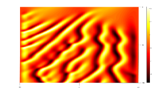
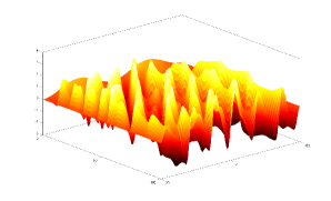
Figure 1. The graph of numerical solution for $N=200$ (spatial nodes) with temporal step $\Delta t=10^{-3}$ and $T=100$. The numerical approximation by the $\theta$/Adams–Bashforth method with $\theta=\frac{3}{4}$ and Lagrange finite elements of order 1.

To see the order of the accuracy between our numerical approximation and the exact solution given above, we let $\Delta t$ decrease from $10^{-1}$ to $10^{-6}$ for large $N=200$, and let $N$ increase from $25$ to $100$ for small $\Delta t=10^{-6}$. The results are given in Table 1. The mathematical study of stability, convergence and accuracy for the above method will be developed in a forthcoming paper.

$\Delta t$	$N$	$L^{\infty}-\mbox{error}$	$L^{2}-\mbox{error}$
$1e{-01}$		$1.32e-02$	$5.54e-06$
$1e{-02}$		$1.13e-03$	$3.46e-08$
$1e{-03}$	200	$8.79e-05$	$2.71e-10$
$1e{-04}$		$5.55e-05$	$5.66e-11$
$1e{-05}$		$5.46e-05$	$6.58e-11$
$1e{-06}$		$5.45e-05$	$6.70e-11$
	25	$3.31e-03$	$1.86e-06$
$1e{-06}$	50	$8.83e-04$	$6.58e-08$
	100	$2.19e-04$	$2.13e-09$

Table 1. Errors in $L^{\infty}$ and $L^{2}$ norms at $T=1s$ using the $\theta$–scheme/Adams–Bashforth method with $\mathbb{P}_{1}$–type Lagrange polynomials (2.22)–(2.24) for the KS equation (2.14).

Now, in order to approximate the solution of the robust control problem, Problem 1, we use as starting point the above discretization schemes as well as the characterization given by Lemma 2.4. Secondly, based in the numerical algorithm proposed in [6, 39] for the Navier–Stokes equations, we propose a similar algorithm for the KS system. Our main novelty relies in the form of constructing the ascent and descent directions, and whose basis is the preconditioned nonlinear gradient conjugate method [34]. The algorithm reads as follows.

Input: Initialize $k=0$ and $(v^{0},\psi^{0})=(0,0)$ on $t\in[0,T]$, where $k$ is the iteration index and $(v^{k},\psi^{k})$ is the numerical approximation of the control and the disturbance during the $k$th iteration of the algorithm.

1 Determine the state $u^{k+1}$ on $[0,T]$ from the KS equation with initial datum $u^{0}$ and the forcing $(v^{k}1_{\mathcal{O}},\psi^{k})$, where $\mathcal{O}\subset(-L,L)$.

2Determine the adjoint state $z^{k+1}$ on $[0,T]$ from the adjoint equation based on the state $u^{k+1}$.

3Determine the local expression of the gradients

$$\frac{DJ_{r}}{Dv}(v^{k},\psi^{k})\quad\mbox{and}\quad\frac{DJ_{r}}{D\psi}(v^{k},\psi^{k}).$$

4Determine the updated disturbance $\psi^{k+1}$ using

$$\psi^{k+1}=\psi^{k}+\alpha^{k}\frac{DJ_{r}}{D\psi}(v^{k},\psi^{k}),$$

where $\alpha^{k}\in(0,1)$ is determined by an iterative procedure described in Remark 2.1.

5Determine the updated control $v^{k+1}$ using

$$v^{k+1}=v^{k}-\beta^{k}\frac{DJ_{r}}{Dv}(v^{k},\psi^{k}),$$

where $\beta^{k}\in(0,1)$ is determined by an iterative procedure described in Remark 2.1.

6Increment index $k=k+1$. Repeat from step 3 until convergence.

Algorithm 1 Robust control algorithm

Remark 2.1.

To find appropriate $\alpha^{k}$ and $\beta^{k}$ directions, we should be able to minimize the following nonlinear functions:

$$f_{k}(\alpha)=J_{r}\Bigl{(}v^{k},\psi^{k}+\alpha\frac{DJ_{r}}{D\psi}(v^{k},\psi^{k})\Bigr{)}\quad\mbox{and}\quad g_{k}(\beta)=J_{r}\Bigl{(}v^{k},v^{k}+\beta\frac{DJ_{r}}{Dv}(v^{k},\psi^{k})\Bigr{)}.$$

Thus, for $k\in\mathbb{N}$, we have

$$f^{\prime}_{k}(\alpha)= \lim\limits_{\varepsilon\to 0}\frac{f_{k}(\alpha+\varepsilon)-f_{k}(\alpha)}{\varepsilon}$$

$$= \lim\limits_{\varepsilon\to 0}\frac{J_{r}(v^{k},\psi^{k}+\alpha\frac{DJ_{r}}{D\psi}(v^{k},\psi^{k})+\varepsilon\frac{DJ_{r}}{D\psi}(v^{k},\psi^{k}))-J_{r}(v^{k},\psi^{k}+\alpha\frac{DJ_{r}}{D\psi}(v^{k},\psi^{k}))}{\varepsilon}$$

$$= \Bigl{\langle}\frac{DJ_{r}}{D\psi}(v^{k},\psi^{k}+\alpha\frac{DJ_{r}}{D\psi}(v^{k},\psi^{k})),\frac{DJ_{r}}{D\psi}(v^{k},\psi^{k})\Bigl{\rangle}_{L^{2}(Q)}.$$

Observe that if $\alpha<<1$, then

$$|f^{\prime}(\alpha)|\simeq\Bigl{\|}\frac{DJ_{r}}{D\psi}(v^{k},\psi^{k})\Bigr{\|}_{L^{2}(Q)}.$$

If $\|\frac{DJ_{r}}{D\psi}(v^{k},\psi^{k})\|_{L^{2}(Q)}>>1$, then we take

$$\alpha^{k+1}=\alpha^{k}-\frac{f^{\prime}_{k}(\alpha^{k})}{\|\frac{DJ_{r}}{D\psi}(v^{k},\psi^{k})\|_{L^{2}(Q)}},$$

otherwise (that is, if $\|\frac{DJ_{r}}{D\psi}(v^{k},\psi^{k})\|_{L^{2}(Q)}\leq 1$), then we take

$$\alpha^{k+1}=\alpha^{k}-f^{\prime}_{k}(\alpha^{k}).$$

In other words, we have consider a preconditioner $P_{k}(x)$ defined by (see [28]):

$$P_{k}(x):=\begin{cases}\displaystyle\frac{x}{\|\frac{DJ_{r}}{D\psi}(v^{k},\psi^{k})\|_{L^{2}(Q)}},&if\,\quad\Bigl{\|}\frac{DJ_{r}}{D\psi}(v^{k},\psi^{k})\Bigr{\|}_{L^{2}(Q)}>1,\\ x,&if\,\quad\Bigl{|}\frac{DJ_{r}}{D\psi}(v^{k},\psi^{k})\Bigr{\|}_{L^{2}(Q)}\leq 1.\end{cases}$$

An analogous procedure is realized for obtaining $\beta^{k}$.

The criterion for the termination of the algorithm is given by

$$\Bigl{\|}\frac{DJ_{r}}{D\psi}(v^{k},\psi^{k})\Bigr{\|}_{L^{2}(Q)}+\Bigl{\|}\frac{DJ_{r}}{Dv^{k}}(v^{k},\psi^{k})\Bigr{\|}_{L^{2}(Q)}<tol,$$

which is analogous to the presented in [39].

Figures 2–7 display numerical results on the robust internal control problem by considering different parameters $\ell$ and $\gamma$ as well as for some functions $u_{d}$. In all experiments, $tol=10^{-6}$, the initial datum is $u^{0}(x)=\sin^{2}\Bigl{(}\frac{\pi x}{30}\Bigr{)}$, $x\in(-30,30)$.

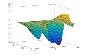
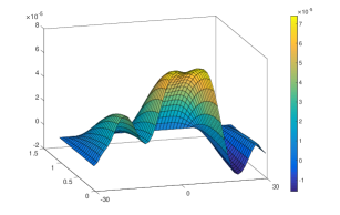
Figure 2. Disturbance signal $\psi$ (left) and control function $v$ (right) on the spatial domain $(-30,30)$. $T=1s,$  $N=50,\Delta t=2\times 10^{-2}$ and $\ell=40,\gamma=40$.

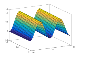
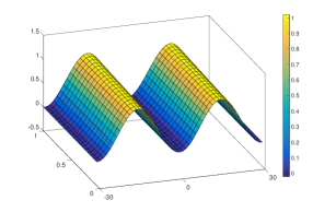
Figure 3. Function $u_{d}(x,t)=\sin^{2}(\frac{\pi x}{30})+10^{-1}t(\cos(\frac{\pi x}{30})+1)$ (left) and state function $u(x,t)$ (right). $T=1s,$  $N=50,\Delta t=2\times 10^{-2}$ and $\ell=40,\gamma=40$.

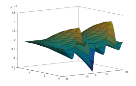
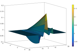
Figure 4. Disturbance signal $\psi$ (left) in the interval $(-30,30)$ and control function $v$ (right) with support in $\mathcal{O}=(-10,10)$. $T=5s,N=50,\Delta t=2\times 10^{-2}$ and $\ell=4,\gamma=400$.

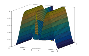
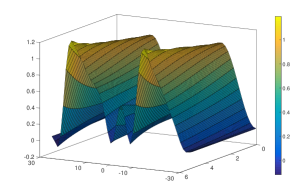
Figure 5. Function $u_{d}(x,t)=\exp(-x^{2})+\sin^{2}(\frac{\pi x}{30})$ (left) and state function $u(x,t)$ (right). $T=5s,N=50,\Delta t=2\times 10^{-2}$ and $\ell=4,\gamma=400$.

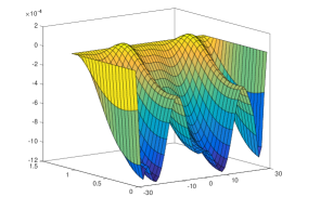
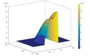
Figure 6. Disturbance signal $\psi$ (left) in the interval $(-30,30)$ and control $v$ (right) with support in $\mathcal{O}=(-10,10)$. $T=1s,N=50,\Delta t=2\times 10^{-2}$ and $\ell=\gamma=10$.

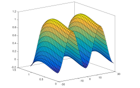
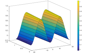
Figure 7. Function $u_{d}(x,t)=(-t^{3}+t^{2})+\sin^{2}(\frac{\pi x}{30})$ (left) and state function $u(x,t)$ (right). $T=1s,N=50,\Delta t=2\times 10^{-2}$ and $\ell=\gamma=10$.

3. Controllability

In the previous section the robust control problem was characterized by a coupled system which needs to be solved. In order to establish a Stackelberg strategy for the case in which the leader control leads the state to the trajectory in a finite time, we must find a function $h\in L^{2}(0,T;L^{2}(\omega))$ such that the corresponding $u$ solution to (1.6) satisfies $u(T)=\overline{u}(T)$, with $\overline{u}$ solution to (1.8). To be precise, to prove the exact controllability to the trajectories, we consider two relevant control systems, namely, the linearized system of (2.13) around $\overline{u}$ which is

$$\begin{cases}u_{t}+u_{xxxx}+u_{xx}+\overline{u}u_{x}+\overline{u}_{x}u=f_{1}+h1_{\omega}+(-\ell^{-2}1_{\mathcal{O}}+\gamma^{-2})z&\text{in }Q,\\ -z_{t}+z_{xxxx}+z_{xx}-(u+\overline{u})z_{x}=f_{2}+(u-u_{d})1_{\mathcal{O}_{d}}&\text{in }Q,\\ u(0,t)=u(1,t)=z(0,t)=z(1,t)=0&\text{on }(0,T),\\ u_{x}(0,t)=u_{x}(1,t)=z_{x}(0,t)=z_{x}(1,t)=0&\text{on }(0,T),\\ u(\cdot,0)=u_{0}(\cdot),\,\,z(\cdot,T)=0&\text{in }(0,1).\end{cases}$$ (3.1)

and the adjoint system associated to (3.1)

$$\left\{\begin{array}[]{lll}\begin{array}[]{llll}-\varphi_{t}+\varphi_{xxxx}+\varphi_{xx}-\overline{u}\varphi_{x}=g_{1}+\theta 1_{\mathcal{O}_{d}}&\text{in }Q,\\ \theta_{t}+\theta_{xxxx}+\theta_{xx}+(\overline{u}\theta)_{x}=g_{2}-\ell^{-2}\varphi 1_{\mathcal{O}}+\gamma^{-2}\varphi&\text{in }Q,\\ \varphi(0,t)=\varphi(1,t)=\theta(0,t)=\theta(1,t)=0&\text{on }(0,T),\\ \varphi_{x}(0,t)=\varphi_{x}(1,t)=\theta_{x}(0,t)=\theta_{x}(1,t)=0&\text{on }(0,T),\\ \varphi(\cdot,T)=\varphi_{T}(\cdot),\,\theta(\cdot,0)=0&\text{in }(0,1).\end{array}\end{array}\right.$$ (3.2)

where $f_{1},f_{2},g_{1},g_{2}$ and $u_{0},\varphi_{T}$ are in appropriate spaces.

Our strategy is as follows:

1. Establish first a global Carleman inequality for the system (3.2). Those inequality allows us to prove a null controllability result for the linearized system (3.1) with right–hand side satisfying suitable decreasing properties near $t=T$.

2. Afterwards, to establish the local exact controllability to the trajectories for the KS system. Here, fixed point arguments will be used.

3.1. Carleman inequalities

We first define some weight functions which will be useful in the sequel. Let $\omega$ and $\omega_{0}$ be non empty subsets of $(0,1)$ such that $\omega_{0}\subset\subset\omega\cap\mathcal{O}_{d}$ and $\eta\in C^{4}([0,1])$ such that

$$|\nabla\eta|>0\mbox{ in }[0,1]\setminus\overline{\omega}_{0},\,\,\,\,\eta>0\mbox{ in }(0,1)\,\,\,\mbox{ and }\,\,\eta(0)=\eta(1)=0.$$

The existence of such a function is proved in [16]. For some positive real number $\lambda$, we consider the weight functions:

$$\begin{array}[]{lll}&\alpha(x,t)=\dfrac{e^{7\lambda\|\eta\|_{\infty}}-e^{\lambda(2\|\eta\|_{\infty}+\eta(x))}}{(t(T-t))^{2/5}},\quad\xi(x,t)=\dfrac{e^{\lambda(2\|\eta\|_{\infty}+\eta(x))}}{(t(T-t))^{2/5}},\\ &\widehat{\alpha}(t)=\max\limits_{x\in[0,1]}\alpha(x,t),\quad\quad\widehat{\xi}(t)=\max\limits_{x\in[0,1]}\xi(x,t),\\ &\breve{\alpha}(t)=\min\limits_{x\in[0,1]}\alpha(x,t),\quad\quad\,\,\,\,\breve{\xi}(t)=\min\limits_{x\in[0,1]}\xi(x,t).\end{array}$$ (3.3)

Henceforth, the constants $a_{0}$ and $m_{0}$ are fixed, and satisfy

$$\frac{5}{4}\leq a_{0}<a_{0}+1<m_{0}<2a_{0},\quad m_{0}<2+a_{0}.$$ (3.4)

Moreover, we will use the following notation for the weighted energy:

$$I_{0}(\rho,u)=\int\limits_{0}^{T}\int\limits_{0}^{1}\rho(s^{-1}\xi^{-1}(|u_{t}|^{2}+|u_{xxxx}|^{2})dxdt+I_{1}(\rho,u),$$

$$I_{1}(\rho,u)=\int\limits_{0}^{T}\int\limits_{0}^{1}\rho(s\lambda^{2}\xi|u_{xxx}|^{2}+s^{3}\lambda^{4}\xi^{3}|u_{xx}|^{2}+s^{5}\lambda^{6}\xi^{5}|u_{x}|^{2}+s^{7}\lambda^{8}\xi^{7}|u|^{2})dxdt,$$

and we also recall the space

$$\mathcal{Z}:=C([0,T];H_{0}^{2}(0,1))\cap L^{2}(0,T;H^{4}(0,1))\cap L^{\infty}(0,T;W^{1,\infty}(0,1)).$$

Our Carleman estimate is given in the the following proposition.

Proposition 3.1.

Let $\overline{u}\in\mathcal{Z}$ and assume that $\omega\cap\mathcal{O}_{d}\neq\emptyset$ and that $\ell$ and $\gamma$ are large enough. Then, there exist a constant $\overline{\lambda}$ such that for any $\lambda\geq\overline{\lambda}$ exist two constants $\overline{s}(\lambda)>0$ and $C=C(\lambda)>0$ depending only on $\omega$ such that for any $g_{1},g_{2}\in L^{2}(Q)$ and any $\varphi_{T}\in L^{2}((0,1))$, the solution of (3.1) satisfies

$$I_{1}(e^{-2s\alpha-2a_{0}s\widehat{\alpha}},\theta)+ I_{0}(e^{-2sm_{0}\alpha},\varphi)\leq C\Biggl{(}s^{15}\lambda^{16}\iint\limits_{\omega\times(0,T)}e^{-2s\breve{\alpha}-2a_{0}s\widehat{\alpha}}(\widehat{\xi})^{29}|\varphi|^{2}dxdt$$ (3.5)

$$+s^{7}\lambda^{8}\iint\limits_{Q}e^{-2s\widehat{\alpha}-2a_{0}s\widehat{\alpha}}(\widehat{\xi})^{7}|g_{1}|^{2}dxdt+s^{7}\lambda^{8}\iint\limits_{Q}e^{-2a_{0}s\widehat{\alpha}}|g_{2}|^{2}dxdt\Biggr{)},$$

for any $s\geq\overline{s}$.

Before giving the proof of Proposition 3.1, we recall some technical results. Let us introduce the system

$$\begin{cases}u_{t}+u_{xxxx}+u_{xx}+\overline{u}u_{x}+\overline{u}_{x}u=f&\text{in }Q,\\ u(0,t)=u(1,t)=u_{x}(0,t)=u_{x}(1,t)=0&\text{on }(0,T),\\ u(\cdot,0)=u_{0}(\cdot)&\text{in }(0,1),\end{cases}$$ (3.6)

where $f\in L^{2}(Q)$ and $\overline{u}\in\mathcal{Z}$.

Lemma 3.2.

Assume $f\in L^{2}(Q)$ and $\omega\subset(0,1)$. Then, there exist positive constants $C(\omega),\,s_{1}$ and $\lambda_{1}$ such that

$$I_{1}(e^{-2s\alpha},u)\leq I_{0}(e^{-2s\alpha},u)\leq C\Bigl{(}\int\limits_{0}^{T}\int\limits_{0}^{1}e^{-2s\alpha}|f|^{2}dxdt+s^{7}\lambda^{8}\int\limits_{0}^{T}\int\limits_{\omega}e^{-2s\alpha}\xi^{7}|u|^{2}dxdt\Bigr{)},$$ (3.7)

for every $s\geq s_{1},\,\lambda\geq\lambda_{1}$, and $u$ solution to (3.6) with $\overline{u}\in\mathcal{Z}$.

Remark 3.1.

Carleman inequality of Lemma 3.2 was proven in [9] with $\overline{u}=0$. However, thanks to the Carleman weight functions and the fact that $\overline{u}\in\mathcal{Z}$ its extension to (3.6) is direct. Besides, in [9] slightly different weight functions are used to prove Lemma 3.2. Nevertheless, the inequality remains valid since the key point of the proof is that $\alpha$ goes to $+\infty$ when $t$ tends to $0$ and $T$. In addition, there exists another Carleman estimate for the system (3.6) (with $\overline{u}=0$) [43]. To our propose is convenient to use [9] instead of [43].

Remark 3.2.

A direct consequence of the weight functions (3.3) shows that, the first term in the right–hand side of (3.7) can be upper bounded by the term $\|e^{-2s\breve{\alpha}+s\widehat{\alpha}}f\|^{2}_{L^{2}(Q)}$. Therefore, (3.7) is transformed in

$$I_{1}(e^{-2s\alpha},u)\leq I_{0}(e^{-2s\alpha},u)\leq C\Bigl{(}\int\limits_{0}^{T}\int\limits_{0}^{1}e^{-4s\breve{\alpha}+2s\widehat{\alpha}}|f|^{2}dxdt+s^{7}\lambda^{8}\int\limits_{0}^{T}\int\limits_{\omega}e^{-2s\alpha}\xi^{7}|u|^{2}dxdt\Bigr{)},$$ (3.8)

for every $s\geq s_{1},\,\lambda\geq\lambda_{1}$, and $u$ solution to (3.6).

Another result holds from the relation between the weight function $\widehat{\alpha}$ and $\breve{\alpha}$. The interested reader can see [32] for more details.

Lemma 3.3.

For any $\varepsilon>0$, any $M_{1},M_{2}\in\mathbb{R}$, there exists $\lambda_{0}>0$ and $C=C(\varepsilon,M_{1},M_{2})>0$ such that

$$e^{s\widehat{\alpha}}\leq Cs^{M_{1}}\lambda^{M_{2}}(\breve{\xi})^{M_{1}}e^{s(1+\varepsilon)\breve{\alpha}},$$ (3.9)

for every $\lambda>\lambda_{0}$.

Remark 3.3.

In relation to Lemma 3.3, it was proven in [32] for $\widehat{\xi}$ instead of $\breve{\xi}$, nevertheless, it is easy to verify that the same arguments holds.

Now, in order to give the proof of Proposition 3.1, we adapt the structure made by Montoya and deTeresa in [32]. More precisely, we must first make a Carleman estimate for $\theta$ with appropriate weight functions. Afterwards, another Carleman inequality for $\varphi$ will be established. The weight functions should be such that all terms respecto to $\theta$ in the right–hand side can be absorbed by the left–hand side. Finally, to estimate local terms of $\theta$, we will use the geometric condition $\mathcal{O}_{d}\cap\omega_{0}\neq\emptyset$.

Proof.

Carleman estimate for $\theta$. Let define $\theta^{*}:=\rho^{*}\theta$, where $\rho^{*}=\rho^{*}(t)=e^{-a_{0}s\widehat{\alpha}}$ and $a_{0}$ fixed satisfying (3.4). From (3.2), $\theta^{*}$ is the solution of the following system

$$\left\{\begin{array}[]{lll}\begin{array}[]{llll}\theta^{*}_{t}+\theta^{*}_{xxxx}+\theta^{*}_{xx}+(\overline{u}\theta^{*})_{x}=\rho^{*}g_{2}+\rho^{*}(-\ell^{-2}\varphi 1_{\mathcal{O}}+\gamma^{-2}\varphi)+\rho^{*}_{t}\theta&\text{in }Q,\\ \theta^{*}(0,t)=\theta^{*}(1,t)=\theta^{*}_{x}(0,t)=\theta^{*}_{x}(1,t)=0&\text{on }(0,T),\\ \theta^{*}(\cdot,0)=0&\text{in }(0,1).\end{array}\end{array}\right.$$

Now, we decompose $\theta^{*}$ as follows:

$$\theta^{*}=\widehat{\theta}+\tilde{\theta},$$ (3.10)

where $\widehat{\theta}$ and $\tilde{\theta}$ solve respectively

$$\left\{\begin{array}[]{lll}\begin{array}[]{llll}\tilde{\theta}_{t}+\tilde{\theta}_{xxxx}+\tilde{\theta}_{xx}+(\overline{u}\tilde{\theta})_{x}=\rho^{*}g_{2}+\rho^{*}(-\ell^{-2}\varphi 1_{\mathcal{O}}+\gamma^{-2}\varphi)&\text{in }Q,\\ \tilde{\theta}(0,t)=\tilde{\theta}(1,t)=\tilde{\theta}_{x}(0,t)=\tilde{\theta}_{x}(1,t)=0&\text{on }(0,T),\\ \tilde{\theta}(\cdot,0)=0&\text{in }(0,1).\end{array}\end{array}\right.$$ (3.11)

and

$$\left\{\begin{array}[]{lll}\begin{array}[]{llll}\widehat{\theta}_{t}+\widehat{\theta}_{xxxx}+\widehat{\theta}_{xx}+(\overline{u}\widehat{\theta})_{x}=\rho^{*}_{t}\theta&\text{in }Q,\\ \widehat{\theta}(0,t)=\widehat{\theta}(1,t)=\widehat{\theta}_{x}(0,t)=\widehat{\theta}_{x}(1,t)=0&\text{on }(0,T),\\ \widehat{\theta}(\cdot,0)=0&\text{in }(0,1).\end{array}\end{array}\right.$$ (3.12)

For system (3.11) we will use Lemma 5.4 (see Appendix 5) with the higher regularity, meanwhile for the system (3.12) we will use some ideas of [32].

Using Lemma 3.2 with $f=\rho^{*}_{t}\theta$ and $u=\widehat{\theta}$, there exists a positive constant $C=C(\omega_{0})$ such that

$$I_{1}(e^{-2s\alpha},\widehat{\theta})\leq C\Bigl{(}\int\limits_{0}^{T}\int\limits_{0}^{1}e^{-2s\alpha}|\rho^{*}_{t}\theta|^{2}dxdt+s^{7}\lambda^{8}\int\limits_{0}^{T}\int\limits_{\omega_{0}}e^{-2s\alpha}\xi^{7}|\widehat{\theta}|^{2}dxdt\Bigr{)},$$ (3.13)

for any $\lambda_{1}:=\lambda\geq C$ and $s\geq s_{1}$.

Now, using the inequality $\frac{a^{2}}{2}-b^{2}\leq(a-b)^{2}$, for every $a,b\in\mathbb{R}$, with $a=\theta^{*}$ and $b=\tilde{\theta}$, we get (recall that $\widehat{\theta}=\theta^{*}-\tilde{\theta}$):

$$\frac{1}{2}I_{1}(e^{-2s\alpha},\theta^{*})-I_{1}(e^{-2s\alpha},\tilde{\theta})\leq I_{1}(e^{-2s\alpha},\widehat{\theta}).$$ (3.14)

Since $s^{7}\lambda^{8}\xi^{7}e^{-2s\alpha}$ is upper bounded, it allows to estimate the terms involved in $I_{1}(e^{-2s\alpha},\tilde{\theta})$ using the regularity inequality (5.6) of Lemma 5.4. In fact, we have:

$$\begin{array}[]{ll}I_{1}(e^{-2s\alpha},\tilde{\theta})&\leq\displaystyle C_{s,\lambda}\|\tilde{\theta}\|^{2}_{L^{2}(0,T;H^{4}(0,1)\cap H_{0}^{2}(0,1))}\\ &\leq C_{s,\lambda}\|\rho^{*}g_{2}\|^{2}_{L^{2}(Q)}+C_{s,\lambda}\|\rho^{*}(-\ell^{-2}\varphi 1_{\mathcal{O}}+\gamma^{-2}\varphi)\|^{2}_{L^{2}(Q)},\end{array}$$ (3.15)

where $C_{s,\lambda}$ is a positive constant depending on $s$ and $\lambda$, i.e., $C_{s,\lambda}=Cs^{7}\lambda^{8}$.

On the other hand, taking into account that $|\rho^{*}_{t}|\leq Cs\rho^{*}(\xi^{*})^{7/2}$ for every $s\geq C$, it follows that

$$\int\limits_{0}^{T}\int\limits_{0}^{1}e^{-2s\alpha}|\rho^{*}_{t}\theta|^{2}dxdt\leq Cs^{2}\int\limits_{0}^{T}\int\limits_{0}^{1}e^{-2s\alpha-2a_{0}s\widehat{\alpha}}(\widehat{\xi})^{7}|\theta|^{2}dxdt,$$

which can be absorbed by the first term in the left–hand side of (3.14), for every $\lambda\geq 1,\,s\geq C$.

Now, to estimate the local term that appear in the right–hand side of (3.13), we use the identity $\theta^{*}=\widehat{\theta}+\tilde{\theta}$ (recall (3.10)). Thus, we have

$$s^{7}\lambda^{8}\int\limits_{0}^{T}\int\limits_{\omega_{0}}e^{-2s\alpha}\xi^{7}|\widehat{\theta}|^{2}dxdt \leq Cs^{7}\lambda^{8}\int\limits_{0}^{T}\int\limits_{\omega_{0}}e^{-2s\alpha}\xi^{7}(|\tilde{\theta}|^{2}+|\theta^{*}|^{2})dxdt$$ (3.16)

$$\leq Cs^{7}\lambda^{8}\int\limits_{0}^{T}\int\limits_{\omega_{0}}e^{-2s\alpha}\xi^{7}|\theta^{*}|^{2}dxdt+C_{s,\lambda}\|\rho^{*}g_{2}\|^{2}_{L^{2}(Q)}$$

$$\hskip 28.45274pt+C_{s,\lambda}\|\rho^{*}(-\ell^{-2}\varphi 1_{\mathcal{O}}+\gamma^{-2}\varphi)\|^{2}_{L^{2}(Q)}.$$

Putting together (3.13)–(3.16), we have for the moment

$$\begin{array}[]{ll}I_{1}(e^{-2s\alpha-2a_{0}s\widehat{\alpha}},\theta)&\leq Cs^{7}\lambda^{8}\displaystyle\int\limits_{0}^{T}\int\limits_{\omega_{0}}e^{-2s\alpha-2a_{0}s\widehat{\alpha}}\xi^{7}|\theta|^{2}dxdt+C_{s,\lambda}\|\rho^{*}g_{2}\|^{2}_{L^{2}(Q)}\\ &\hskip 28.45274pt+C_{s,\lambda}\|\rho^{*}(-\ell^{-2}\varphi 1_{\mathcal{O}}+\gamma^{-2}\varphi)\|^{2}_{L^{2}(Q)},\end{array}$$ (3.17)

for every $s\geq C$ and $\lambda_{1}:=\lambda\geq C$.

Carleman estimate for $\varphi$. First, assuming that $\theta$ is given, we look at $\varphi$ as the solution of

$$\left\{\begin{array}[]{lll}\begin{array}[]{llll}-\varphi_{t}+\varphi_{xxxx}+\varphi_{xx}-\overline{u}\varphi_{x}=g_{1}+\theta 1_{\mathcal{O}_{d}}&\text{in }Q,\\ \varphi(0,t)=\varphi(1,t)=\varphi_{x}(1,t)=\varphi_{x}(0,t)=0&\text{on }(0,T),\\ \varphi(\cdot,T)=\varphi_{T}(\cdot)&\text{in }(0,1).\end{array}\end{array}\right.$$ (3.18)

Applying Lemma 3.2 jointly with its remark 3.2 for $f=g_{1}+\theta 1_{\mathcal{O}_{d}}$ and the weight function $m_{0}\alpha$ (instead of $\alpha$), where $a_{0}+1<m_{0}\leq 2a_{0}$ and $m_{0}\leq 2+a_{0}$, we obtain

$$\begin{array}[]{lll}I_{0}(e^{-2m_{0}s\alpha},\varphi)&\leq C\Biggl{(}\displaystyle\int\limits_{0}^{T}\int\limits_{0}^{1}e^{-4m_{0}s\breve{\alpha}+2m_{0}s\widehat{\alpha}}|g_{1}|^{2}dxdt+\displaystyle\int\limits_{0}^{T}\int\limits_{\mathcal{O}_{d}}e^{-4m_{0}s\breve{\alpha}+2m_{0}s\widehat{\alpha}}|\theta|^{2}dxdt\\ &\hskip 28.45274pt+s^{7}\lambda^{8}\displaystyle\int\limits_{0}^{T}\int\limits_{\omega_{0}}e^{-2m_{0}s\alpha}\xi^{7}|\varphi|^{2}dxdt\Biggr{)},\end{array}$$ (3.19)

for any $\lambda_{2}:=\lambda\geq C$ and $s\geq C$.

By considering Lemma 3.3 with $\varepsilon=\frac{m_{0}-a_{0}-1}{m_{0}+a_{0}+1}$, $M_{1}=\frac{7}{2(m_{0}+a_{0}+1)}$ and $M_{2}=\frac{4}{(m_{0}+a_{0}+1)}$, the second term in the right–hand side of (3.19) can be estimated by $I_{1}(e^{-2s\widehat{\alpha}-2a_{0}s\widehat{\alpha}},\theta)$ and therefore it can be absorbed by the left–hand side of (3.17).

From (3.17) and (3.19) we have

$$I_{1}(e^{-2s\alpha-2a_{0}s\widehat{\alpha}},\theta)+I_{0}(e^{-2m_{0}s\alpha},\varphi)$$ (3.20)

$$\leq Cs^{7}\lambda^{8}\int\limits_{0}^{T}\int\limits_{\omega_{0}}e^{-2m_{0}s\alpha}\xi^{7}|\varphi|^{2}dxdt+Cs^{7}\lambda^{8}\int\limits_{0}^{T}\int\limits_{\omega_{0}}e^{-2s\alpha-2a_{0}s\widehat{\alpha}}\xi^{7}|\theta|^{2}dxdt+C_{s,\lambda}\|\rho^{*}g_{2}\|^{2}_{L^{2}(Q)}$$

$$\hskip 28.45274pt+C\int\limits_{0}^{T}\int\limits_{0}^{L}e^{-4m_{0}s\breve{\alpha}+2m_{0}s\widehat{\alpha}}|g_{1}|^{2}dxdt+C_{s,\lambda}\|\rho^{*}(-\ell^{-2}\varphi 1_{\mathcal{O}}+\gamma^{-2}\varphi)\|^{2}_{L^{2}(Q)},$$

for any $\lambda_{3}:=\max\{\lambda_{1},\lambda_{2}\}\geq C,\,s\geq C$ and $C_{s,\lambda}$ depending on $s,\lambda$.

Taking $\ell$ and $\gamma$ large enough, i.e., $\ell,\gamma>C_{1}T^{14/10}e^{C_{2}/T^{4/5}}$, where $C_{1},\,C_{2}$ are positive constants depending on $a_{0},m_{0},s$, we can absorb the last term in the right–hand side of (3.20) by the left–hand side.

Finally, we should estimate the local term concerning $\theta$ in terms of $\varphi$. The idea is to use the first equation of (3.18) and the hypothesis $\omega\cap\mathcal{O}_{d}\neq\emptyset$, where $\omega_{0}\subset\omega\subset\mathcal{O}_{d}$. Thus, we introduce an open set $\omega_{1}\subset\omega$ such that $\omega_{0}\subset\omega_{1}$ and a positive function $\zeta\in C^{4}_{c}(\omega_{1})$ such that $\zeta\equiv 1$ in $\omega_{0}$. Then, by using (3.18) and after several integration by parts in time and space we get:

$$J =s^{7}\lambda^{8}\int\limits_{0}^{T}\int\limits_{\omega_{0}}e^{-2s\alpha-2a_{0}s\widehat{\alpha}}\xi^{7}|\theta|^{2}dxdt$$

$$\leq Cs^{7}\lambda^{8}\int\limits_{0}^{T}\int\limits_{\omega_{1}}\zeta e^{-2s\alpha-2a_{0}s\widehat{\alpha}}\xi^{7}(-\varphi_{t}+\varphi_{xxxx}+\varphi_{xx}-\overline{u}\varphi_{x}-g_{1})\theta dxdt$$

$$=C\Biggl{(}s^{7}\lambda^{8}\int\limits_{0}^{T}\int\limits_{\omega_{1}}\zeta(e^{-2s\alpha-2a_{0}s\widehat{\alpha}}\xi^{7})_{t}\varphi\theta dxdt$$

$$+s^{7}\lambda^{8}\int\limits_{0}^{T}\int\limits_{\omega_{1}}\zeta e^{-2s\alpha-2a_{0}s\widehat{\alpha}}\xi^{7}(\theta_{t}+\theta_{xxxx}+\theta_{xx}+(\overline{u}\theta)_{x})\varphi dxdt$$

$$+s^{7}\lambda^{8}\int\limits_{0}^{T}\int\limits_{\omega_{1}}(\zeta e^{-2s\alpha-2a_{0}s\widehat{\alpha}}\xi^{7})_{xxxx}\varphi\theta dxdt+s^{7}\lambda^{8}\int\limits_{0}^{T}\int\limits_{\omega_{1}}(\zeta e^{-2s\alpha-2a_{0}s\widehat{\alpha}}\xi^{7})_{xxx}\varphi\theta_{x}dxdt$$

$$+s^{7}\lambda^{8}\int\limits_{0}^{T}\int\limits_{\omega_{1}}(\zeta e^{-2s\alpha-2a_{0}s\widehat{\alpha}}\xi^{7})_{xx}(\varphi\theta_{xx}+\varphi\theta)dxdt$$

$$+s^{7}\lambda^{8}\int\limits_{0}^{T}\int\limits_{\omega_{1}}(\zeta e^{-2s\alpha-2a_{0}s\widehat{\alpha}}\xi^{7})_{x}(\varphi\theta_{xxx}+\varphi\theta_{x}+\overline{u}\varphi\theta)dxdt.\Biggr{)}$$

Now, using the estimates

$$|\partial_{x}^{k}(\zeta e^{-2s\alpha-2a_{0}s\widehat{\alpha}}\xi^{7})|\leq Cs^{k}\lambda^{k}\xi^{8+\frac{5k}{2}}e^{-2s\alpha-2a_{0}s\widehat{\alpha}},\quad k=1,\dots,4,$$

$$|\partial_{t}(e^{-2s\alpha-2a_{0}s\widehat{\alpha}}\xi^{7})|\leq CTe^{-2s\alpha-2a_{0}s\widehat{\alpha}}\xi^{\frac{21}{2}},$$

as well as the equation related to $\theta$ (see (3.2)) and the fact that $\overline{u}\in L^{\infty}(0,T;W^{1,\infty}(0,1))$, the term $J$ can be estimated as follows:

$$J \leq C\Biggl{(}s^{7}\lambda^{8}\int\limits_{0}^{T}\int\limits_{\omega_{1}}\zeta e^{-2s\alpha-2a_{0}s\widehat{\alpha}}\xi^{\frac{21}{2}}|\varphi||\theta|dxdt$$

$$\quad+s^{7}\lambda^{8}\int\limits_{0}^{T}\int\limits_{\omega_{1}}\zeta e^{-2s\alpha-2a_{0}s\widehat{\alpha}}\xi^{7}(g_{2}-\ell^{-2}\varphi 1_{\mathcal{O}}+\gamma^{-2}\varphi)\varphi dxdt$$

$$\quad+s^{11}\lambda^{12}\int\limits_{0}^{T}\int\limits_{\omega_{1}}e^{-2s\alpha-2a_{0}s\widehat{\alpha}}\xi^{18}|\varphi||\theta|dxdt+s^{10}\lambda^{11}\int\limits_{0}^{T}\int\limits_{\omega_{1}}e^{-2s\alpha-2a_{0}s\widehat{\alpha}}\xi^{\frac{31}{2}}|\varphi||\theta_{x}|dxdt$$

$$\quad+s^{9}\lambda^{10}\int\limits_{0}^{T}\int\limits_{\omega_{1}}e^{-2s\alpha-2a_{0}s\widehat{\alpha}}\xi^{13}|\varphi||\theta_{xx}|dxdt+s^{8}\lambda^{9}\int\limits_{0}^{T}\int\limits_{\omega_{1}}e^{-2s\alpha-2a_{0}s\widehat{\alpha}}\xi^{\frac{21}{2}}|\varphi||\theta_{xxx}|dxdt\Biggr{)},$$

with $C$ depending on $T$ and $\|\overline{u}\|_{L^{\infty}(0,T;W^{1,\infty}(0,1))}$.

Taking into account that $\omega\cap\mathcal{O}=\emptyset$ and applying Young’s inequality at each term of the previous inequality, it is easy to deduce the following inequality:

$$J \leq\varepsilon I_{1}(e^{-2s\alpha-2a_{0}s\widehat{\alpha}},\theta)+C(\varepsilon)s^{15}\lambda^{16}\int\limits_{0}^{T}\int\limits_{\omega_{1}}e^{-2s\breve{\alpha}-2a_{0}s\widehat{\alpha}}(\widehat{\xi})^{29}|\varphi|^{2}dxdt$$ (3.21)

$$\quad+C(\varepsilon)s^{7}\lambda^{8}\int\limits_{0}^{T}\int\limits_{0}^{1}e^{-2s\alpha-2a_{0}s\widehat{\alpha}}\xi^{7}|g_{1}|^{2}dxdt+Cs^{7}\lambda^{8}\int\limits_{0}^{T}\int\limits_{0}^{1}e^{-2a_{0}s\widehat{\alpha}}|g_{2}|^{2}dxdt$$

$$\quad+Cs^{14}\lambda^{16}\int\limits_{0}^{T}\int\limits_{\omega_{1}}e^{-4s\alpha-2a_{0}s\widehat{\alpha}}\xi^{14}|\varphi|^{2}dxdt,$$

for every $s\geq C,\,\varepsilon>0,\,\ell>0$ and $\gamma$ large enough.

From the definition of $\breve{\alpha},\,\widehat{\alpha}$ and $\widehat{\xi}$ (see (3.3)), the second term in the right–hand side can estimate both the last term in the right–hand side and the first term in the right–hand side of (3.20). In fact, the first affirmation holds for every $s\geq 1$, meanwhile the second one is a consequence of using Lemma 3.3 with $\varepsilon=((m_{0}-1)/a_{0})-1$ and $M_{1}=M_{2}=4/a_{0}$. Therefore, from (3.20) and (3.21), we conclude the proof of Proposition 3.1. ∎

3.2. Null controllability of the linearized system

In this subsection we will prove the null controllability for the coupled system (3.1) with a right–hand side with external sources decreasing exponentially to zero when $t$ goes to $T$. In other words, we would like to find $h\in L^{2}(0,T;L^{2}(\omega))$ such that the solution of

$$\begin{cases}u_{t}+u_{xxxx}+u_{xx}+\overline{u}u_{x}+\overline{u}_{x}u=f_{1}+h1_{\omega}+(-\ell^{-2}1_{\mathcal{O}}+\gamma^{-2})z&\text{in }Q,\\ -z_{t}+z_{xxxx}+z_{xx}-(u+\overline{u})z_{x}=f_{2}+(u-u_{d})1_{\mathcal{O}_{d}}&\text{in }Q,\\ u(0,t)=u(1,t)=z(0,t)=z(1,t)=0&\text{on }(0,T),\\ u_{x}(0,t)=u_{x}(1,t)=z_{x}(0,t)=z_{x}(1,t)=0&\text{on }(0,T),\\ u(\cdot,0)=u_{0}(\cdot),\,\,z(\cdot,T)=0&\text{in }(0,1).\end{cases}$$ (3.22)

satisfies

$$u(\cdot,T)=0\quad\mbox{in }(0,1),$$ (3.23)

where the functions $f_{1}$ and $f_{2}$ are in appropriate weighted spaces. To this end, let us first state a Carleman inequality with weight functions not vanishing in $t=0$. Thus, let $\tilde{\ell}\in C^{1}([0,T])$ be a positive function in $[0,T)$ such that:

$$\tilde{\ell}(t)=T^{2}/4\quad\forall t\in[0,T/2]\ \text{ and }\ \tilde{\ell}(t)=t(T-t)\quad\forall t\in[T/2,T].$$

Now, we introduce the following weight functions

$$\begin{array}[]{ll}&\beta(x,t)=\dfrac{e^{7\lambda\|\eta\|_{\infty}}-e^{\lambda(2\|\eta\|_{\infty}+\eta(x))}}{\tilde{\ell}^{2/5}(t)},\quad\tau(x,t)=\dfrac{e^{\lambda(2\|\eta\|_{\infty}+\eta(x))}}{\tilde{\ell}^{2/5}(t)},\\ &\widehat{\beta}(t)=\max\limits_{x\in[0,1]}\beta(x,t),\quad\quad\breve{\tau}(t)=\min\limits_{x\in[0,1]}\tau(x,t),\\ &\breve{\beta}(t)=\min\limits_{x\in[0,1]}\beta(x,t),\quad\quad\,\,\,\,\widehat{\tau}(t)=\max\limits_{x\in[0,1]}\tau(x,t).\end{array}$$ (3.24)

Lemma 3.4.

Let $s$ and $\lambda$ like in Theorem 3.1. Then, there exists a constant $C>0$ depending on $s,\lambda,\omega,T$ and $\|\overline{u}\|_{L^{\infty}(0,T;W^{1,\infty}(0,1))}$, such that every solution $(\varphi,\theta)$ of (3.2) satisfies

$$\begin{array}[]{ll}\|\varphi(\cdot,0)\|^{2}_{L^{2}(0,L)}+\displaystyle\iint\limits_{Q}e^{-2m_{0}s\widehat{\beta}}(\breve{\tau})^{7}|\varphi|^{2}dxdt\\ \hskip 28.45274pt+\displaystyle\iint\limits_{Q}e^{-2(a_{0}+1)s\widehat{\beta}}(\breve{\tau})^{7}|\theta|^{2}dxdt+\displaystyle\iint\limits_{Q}e^{-4a_{0}s\widehat{\beta}}(\breve{\tau})^{7}|\theta|^{2}dxdt\\ \leq C\Biggl{(}\displaystyle\iint\limits_{Q}e^{-2a_{0}s\widehat{\beta}}(\widehat{\tau})^{7}|g_{1}|^{2}dxdt+\displaystyle\iint\limits_{Q}e^{-2a_{0}s\widehat{\beta}}|g_{2}|^{2}dxdt+\displaystyle\iint\limits_{\omega\times(0,T)}e^{-2s\breve{\beta}-2a_{0}s\widehat{\beta}}(\widehat{\tau})^{29}|\varphi|^{2}dxdt\Biggr{)}.\end{array}$$ (3.25)

Proof.

The proof follows from classical energy estimates and therefore it is omitted. The interested reader might see for instance [32, Lemma 3.4] for more details. ∎

Now, we look for a solution of (3.22) in an appropriate weighted functional space.

Let us define the space $E$ as follows:

$$\begin{array}[]{ll}E:=&\Bigl{\{}(u,z,h):e^{a_{0}s\widehat{\beta}}(\widehat{\tau})^{-7/2}u\in L^{2}(Q),e^{a_{0}s\widehat{\beta}}z\in L^{2}(Q),\\ &\hskip 14.22636pte^{a_{0}s\widehat{\beta}+s\breve{\beta}}(\widehat{\tau})^{-29/2}h1_{\omega}\in L^{2}(Q),\\ &\hskip 14.22636pte^{a_{0}s\widehat{\beta}}(\widehat{\tau})^{-29/2}u\in L^{2}(0,T;H^{2}(0,1))\cap L^{\infty}(0,T;L^{2}(0,1)),\\ &\hskip 14.22636pte^{a_{0}s\widehat{\beta}}(\breve{\tau})^{-c_{0}}z\in L^{2}(0,T;H^{2}(0,1))\cap L^{\infty}(0,T;L^{2}(0,1)),\,\,c_{0}\geq\frac{9}{2},\\ &\hskip 14.22636pte^{m_{0}s\widehat{\beta}}(\breve{\tau})^{-7/2}(u_{t}+u_{xxxx}+u_{xx}+(\overline{u}u)_{x}-h1_{\omega}-(-\ell^{-2}1_{\mathcal{O}}+\gamma^{-2})z)\in L^{2}(Q),\\ &\hskip 14.22636pte^{2a_{0}s\widehat{\beta}}(\breve{\tau})^{-7/2}(-z_{t}+z_{xxxx}+z_{xx}-(u+\overline{u})z_{x}-(u-u_{d})1_{\mathcal{O}_{d}})\in L^{2}(Q)\Bigr{\}}.\end{array}$$

Proposition 3.5.

Assume the hypotheses of Lemma 3.4 and

$$u_{0}\in L^{2}(0,1),\,e^{m_{0}s\widehat{\beta}}(\breve{\tau})^{-7/2}f_{1}\in L^{2}(Q),\,\,e^{2a_{0}s\widehat{\beta}}(\breve{\tau})^{-7/2}f_{2}\in L^{2}(Q),$$ (3.26)

$$\iint\limits_{\mathcal{O}_{d}\times(0,T)}\rho^{2}(t)|u_{d}|^{2}dxdt<+\infty,$$ (3.27)

where $\rho=\rho(t)$ is a positive function blowing up $t=T$. Then, there exists a control $h\in L^{2}(0,T;L^{2}(\omega))$ such that the associated solution $(u,z,h)$ to (3.22) satisfies $(u,z,h)\in E$.

Proof of Proposition 3.5.

Let us introduce the following constrained extremal problem:

$$\begin{array}[]{lll}\inf&\left\{\begin{array}[]{lll}&\displaystyle\frac{1}{2}\Bigl{(}\iint\limits_{Q}e^{2a_{0}s\widehat{\beta}}(\widehat{\tau})^{-7}|u|^{2}dxdt+\iint\limits_{Q}e^{2a_{0}s\widehat{\beta}}|z|^{2}dxdt\\ &\hskip 28.45274pt+\displaystyle\iint\limits_{\omega\times(0,T)}e^{2(a_{0}s\widehat{\beta}+s\breve{\beta})}(\widehat{\tau})^{-29}|h|^{2}dxdt\Bigr{)}\end{array}\right.\\ &\mbox{subject to}\,\,h\in L^{2}(Q),\,\,supp\,h\subset\omega\times(0,T),\,\,\mbox{and}\,\,\eqref{eq.ks.controllineal}.\\ &\end{array}$$ (3.28)

Assume that this problem admits a unique solution $(\widehat{u},\widehat{z},\widehat{h})$. Then, from Lagrange’s principle there exists dual variables $(\widehat{\varphi},\widehat{\theta})$ such that

$$\begin{array}[]{llll}&\widehat{u}=e^{-2a_{0}s\widehat{\beta}}(\widehat{\tau})^{7}(-\widehat{\varphi}_{t}+\widehat{\varphi}_{xxxx}+\widehat{\varphi}_{xx}-\overline{u}\widehat{\varphi}_{x}-\widehat{\theta}1_{\mathcal{O}_{d}})&\mbox{in}&Q,\\ &\widehat{z}=e^{-2a_{0}s\widehat{\beta}}(\widehat{\theta}_{t}+\widehat{\theta}_{xxxx}+\widehat{\theta}_{xx}+(\overline{u}\widehat{\theta})_{x}-(-\ell^{-2}\chi_{\mathcal{O}}+\gamma^{-2})\widehat{\varphi})&\mbox{in}&Q,\\ &\widehat{h}=e^{-2(a_{0}s\widehat{\beta}+s\breve{\beta})}(\widehat{\tau})^{29}\widehat{\varphi}&\mbox{in}&Q,\\ &\widehat{u}=\widehat{z}=0&\mbox{on}&\{0,1\}\times(0,T).\end{array}$$ (3.29)

Let us now set the space

$$P_{0}:\{(u,z)\in C^{4}(\overline{Q}):\partial_{x}^{k}u(0,t)=\partial_{x}^{k}u(1,t)=\partial_{x}^{k}z(0,t)=\partial_{x}^{k}z(1,t)=0,\quad k=0,1\}.$$

as well as the bilinear form $a(\cdot,\cdot)$ over $P_{0}\times P_{0}$ defined by:

$$\begin{array}[]{ll}&\displaystyle\iint\limits_{Q}e^{-2a_{0}s\widehat{\beta}}(\widehat{\tau})^{7}(-\widehat{\varphi}_{t}+\widehat{\varphi}_{xxxx}+\widehat{\varphi}_{xx}-\overline{u}\widehat{\varphi}_{x}-\widehat{\theta}1_{\mathcal{O}_{d}})(-w_{t}+w_{xxxx}+w_{xx}-\overline{u}w_{x}-z1_{\mathcal{O}_{d}})\,dxdt\\ &+\displaystyle\iint\limits_{Q}e^{-2a_{0}s\widehat{\beta}}(\widehat{\theta}_{t}+\widehat{\theta}_{xxxx}+\widehat{\theta}_{xx}+(\overline{u}\widehat{\theta})_{x}-(-\ell^{-2}\chi_{\mathcal{O}}+\gamma^{-2})\widehat{\varphi})(z_{t}+z_{xxxx}+z_{xx}+(\overline{u}z)_{x})\\ &-\displaystyle\iint\limits_{Q}e^{-2a_{0}s\widehat{\beta}}(\widehat{\theta}_{t}+\widehat{\theta}_{xxxx}+\widehat{\theta}_{xx}+(\overline{u}\widehat{\theta})_{x}-(-\ell^{-2}\chi_{\mathcal{O}}+\gamma^{-2})(-\ell^{-2}\chi_{\mathcal{O}}+\gamma^{-2})w)\,dxdt\\ &+\displaystyle\iint\limits_{\omega\times(0,T)}e^{-2(a_{0}s\widehat{\beta}+s\breve{\beta})}(\widehat{\tau})^{29}\widehat{\varphi}w\,dxdt=:a((\widehat{\varphi},\widehat{\theta}),(w,z)),\end{array}$$

for every $(w,z)\in P_{0}$, and a linear form

$$\langle G,(w,z)\rangle:=\displaystyle\iint\limits_{Q}f_{1}\cdot w\,dxdt+\displaystyle\iint\limits_{Q}f_{2}\cdot z\,dxdt+\displaystyle\int\limits_{\Omega}u_{0}(\cdot)\cdot w(\cdot,0)\,dx.$$ (3.30)

Taking into account these definitions, one can see that, if the functions $\widehat{u},\widehat{z}$ and $\widehat{h}$ solve (3.28), we must have for every $(w,z)$ in $P_{0}$

$$a((\widehat{\varphi},\widehat{\theta}),(w,z))=\langle G,(w,z)\rangle.$$ (3.31)

Note that Carleman inequality (3.25) holds for all $(w,z)\in P_{0}$. Consequently,

$$\begin{array}[]{ll}&\|w(\cdot,0)\|^{2}_{L^{2}(0,L)}+\displaystyle\iint\limits_{Q}e^{-2m_{0}s\widehat{\beta}}(\breve{\tau})^{7}|w|^{2}dxdt\\ &\hskip 28.45274pt+\displaystyle\iint\limits_{Q}e^{-2(a_{0}+1)s\widehat{\beta}}(\breve{\tau})^{7}|z|^{2}dxdt+\displaystyle\iint\limits_{Q}e^{-4a_{0}s\widehat{\beta}}(\breve{\tau})^{7}|z|^{2}dxdt\leq Ca((w,z),(w,z)),\end{array}$$ (3.32)

for every $(w,z)\in P_{0}$.
Therefore, it is easy to prove that $a(\cdot,\cdot):P_{0}\times P_{0}\longmapsto\mathbb{R}$ is symmetric, definite positive bilinear form on $P_{0}$, so that, by defining $P$ as the completion of $P_{0}$ for the norm induced by $a(\cdot,\cdot)$ it implies that $a(\cdot,\cdot)$ is well–defined, continuous and again definite positive on $P$. In addition, from Carleman inequality (3.25), the hypothesis over the functions $f_{1}$ and $f_{2}$ (see (3.26)), and (3.32), the linear form $(w,z)\longmapsto\langle G,(w,z)\rangle$ is well–defined and continuous on $P$. Indeed, thanks to the relation among $a_{,}m_{0}$, see (3.4), for every $(w,z)\in P$ we have

$$\langle G,(w,z)\rangle \leq\|e^{(a_{0}+1)s\widehat{\beta}}(\breve{\tau})^{-7/2}f_{1}\|_{L^{2}(Q)}\|e^{-(a_{0}+1)s\widehat{\beta}}(\breve{\tau})^{7/2}w\|_{L^{2}(Q)}$$

$$\hskip 14.22636pt+\|e^{m_{0}s\widehat{\beta}}(\breve{\tau})^{-7/2}f_{2}\|_{L^{2}(Q)}\|e^{-m_{0}s\widehat{\beta}}(\breve{\tau})^{7/2}z\|_{L^{2}(Q)}+\|u_{0}\|_{L^{2}(0,1)}\|w(0)\|_{L^{2}(0,1)}$$

$$\leq\|e^{m_{0}s\widehat{\beta}}(\breve{\tau})^{-7/2}f_{1}\|_{L^{2}(Q)}\|e^{-(a_{0}+1)s\widehat{\beta}}(\breve{\tau})^{7/2}w\|_{L^{2}(Q)}$$

$$\hskip 14.22636pt+\|e^{2a_{0}s\widehat{\beta}}(\breve{\tau})^{-7/2}f_{2}\|_{L^{2}(Q)}\|e^{-m_{0}s\widehat{\beta}}(\breve{\tau})^{7/2}z\|_{L^{2}(Q)}+\|u_{0}\|_{L^{2}(0,1)}\|w(0)\|_{L^{2}(0,1)}.$$

Using (3.32) and the density of $P_{0}$ in $P$, we find

$$\langle G,(w,z)\rangle\leq C\Bigl{(}\|e^{m_{0}s\widehat{\beta}}(\breve{\tau})^{-7/2}f_{1}\|_{L^{2}(Q)}+\|e^{2a_{0}s\widehat{\beta}}(\breve{\tau})^{-7/2}f_{2}\|_{L^{2}(Q)}+\|y_{0}\|_{L^{2}(0,1)}\Bigr{)}\|(w,z)\|_{P}.$$

Hence, from Lax–Milgram’s Lemma, there exists a unique $(\widehat{\varphi},\widehat{\theta})\in P$ satisfying

$$a((\widehat{\varphi},\widehat{\theta}),(w,z))=\langle G,(w,z)\rangle,\quad\forall(w,z)\in P.$$ (3.33)

Let us set $(\widehat{u},\widehat{z},\widehat{h})$ like in (3.29) and remark that $(\widehat{u},\widehat{z},\widehat{h})$ verifies

$$\begin{array}[]{ll}a((\widehat{\varphi},\widehat{\theta}),(\widehat{\varphi},\widehat{\theta}))=\displaystyle\iint\limits_{Q}e^{2a_{0}s\widehat{\beta}}(\widehat{\tau})^{-7}|\widehat{u}|^{2}dxdt\\ +\displaystyle\iint\limits_{Q}e^{2a_{0}s\widehat{\beta}}|\widehat{z}|^{2}dxdt+\displaystyle\iint\limits_{\omega\times(0,T)}e^{2(a_{0}s\widehat{\beta}+s\breve{\beta})}(\widehat{\tau})^{-29}|\widehat{h}|^{2}dxdt<+\infty.\end{array}$$ (3.34)

Let us prove that $(\widehat{u},\widehat{z})$ is the weak solution of the coupled system (3.22) for $h=\widehat{h}$. In fact, we introduce the (weak) solution $(\tilde{u},\tilde{z})$ to the coupled system

$$\begin{cases}\tilde{u}_{t}+\tilde{u}_{xxxx}+\tilde{u}_{xx}+\overline{u}\tilde{u}_{x}+\overline{u}_{x}\tilde{u}=f_{1}+h1_{\omega}+(-\ell^{-2}1_{\mathcal{O}}+\gamma^{-2})\tilde{z}&\text{in }Q,\\ -\tilde{z}_{t}+\tilde{z}_{xxxx}+\tilde{z}_{xx}-(\tilde{u}+\overline{u})\tilde{z}_{x}=f_{2}+(\tilde{u}-u_{d})1_{\mathcal{O}_{d}}&\text{in }Q,\\ \tilde{u}(0,t)=\tilde{u}(1,t)=\tilde{z}(0,t)=\tilde{z}(1,t)=0&\text{on }(0,T),\\ \tilde{u}_{x}(0,t)=\tilde{u}_{x}(1,t)=\tilde{z}_{x}(0,t)=\tilde{z}_{x}(1,t)=0&\text{on }(0,T),\\ \tilde{u}(\cdot,0)=\tilde{u}_{0}(\cdot),\,\,\tilde{z}(\cdot,T)=0&\text{in }(0,1).\end{cases}$$ (3.35)

Clearly, $(\tilde{u},\tilde{z})$ is the unique solution of (3.35) defined by transposition. This means that, for every $(a,b)\in L^{2}(Q)^{2}$,

$$\langle(\tilde{u},\tilde{z}),(a,b)\rangle_{L^{2}(Q)^{2}}=\langle u_{0},\varphi(0)\rangle_{L^{2}((0,1))}+\langle(f_{1}+\widehat{h}1_{\omega},f_{2}),(\varphi,\theta)\rangle_{L^{2}(Q)^{2}},$$ (3.36)

where $(\varphi,\theta)$ is the solution to

$$\left\{\begin{array}[]{lll}L^{*}(\varphi,\theta)=(a,b)&\text{ in }Q,\\ \varphi(0,t)=\varphi(1,t)=\theta(0,t)=\theta(1,t)=0&\text{on }(0,T),\\ \varphi_{x}(0,t)=\varphi_{x}(1,t)=\theta_{x}(0,t)=\theta_{x}(1,t)=0&\text{on }(0,T),\\ \varphi(\cdot,T)=\varphi_{T}(\cdot),\,\theta(\cdot,0)=0&\text{in }(0,1)\end{array}\right.$$ (3.37)

and $L^{*}$ is the adjoint operator of $L$ given by:

$$L(\tilde{u},\tilde{z})=(L_{1}(\tilde{u},\tilde{z}),L_{2}(\tilde{u},\tilde{z})),$$

with

$$L_{1}(\tilde{u},\tilde{z})=\tilde{u}_{t}+\tilde{u}_{xxxx}+\tilde{u}_{xx}+\overline{u}\tilde{u}_{x}+\overline{u}_{x}\tilde{u}-(-\ell^{-2}1_{\mathcal{O}}+\gamma^{-2})\tilde{z}$$

and

$$L_{2}(\tilde{u},\tilde{z})=-\tilde{z}_{t}+\tilde{z}_{xxxx}+\tilde{z}_{xx}-(\tilde{u}+\overline{u})\tilde{z}_{x}-(\tilde{u}-u_{d})1_{\mathcal{O}_{d}}.$$

From (3.29) and (3.31), we see that $(\widehat{u},\widehat{z})$ also satisfies (3.36). Then $(\widehat{u},\widehat{z})=(\tilde{u},\tilde{z})$ is the weak solution to (3.35).

Finally, we must see that $(\widehat{u},\widehat{z},\widehat{h})\in E$. Observe that from (3.34), we have that

$$e^{a_{0}s\widehat{\beta}}(\widehat{\tau})^{-7/2}\widehat{u},\,\,e^{a_{0}s\beta^{*}}\widehat{z},\,\,\,e^{(a_{0}s\widehat{\beta}+s\breve{\beta})}(\widehat{\tau})^{-29/2}\widehat{h}1_{\omega}\in L^{2}(Q)$$

and by hypothesis (3.26)

$$e^{m_{0}s\widehat{\beta}}(\breve{\tau})^{-7/2}f_{1}\in L^{2}(Q)\quad\mbox{and}\quad e^{2a_{0}s\widehat{\beta}}(\breve{\tau})^{-7/2}f_{2}\in L^{2}(Q).$$

Thus, it only remains to check that

$$e^{a_{0}s\widehat{\beta}}(\widehat{\tau})^{-29/2}\widehat{u},\,\,e^{a_{0}s\widehat{\beta}}(\breve{\tau})^{-c_{0}}\widehat{z}\in L^{2}(0,T;H^{2}(0,1))\cap L^{\infty}(0,T;L^{2}(0,1)),$$

where $c_{0}\geq\frac{9}{2}.$

1. We define the functions

   $$\begin{array}[]{llll}u^{*}:=e^{a_{0}s\widehat{\beta}}(\widehat{\tau})^{-29/2}\widehat{u},&&z^{*}:=e^{a_{0}s\widehat{\beta}}(\breve{\tau})^{-c_{0}}\widehat{z}\\ \end{array}$$

   and

   $$\begin{array}[]{llll}f^{*}_{1}:=e^{a_{0}s\widehat{\beta}}(\widehat{\tau})^{-29/2}(f_{1}+h1_{\omega}),&&z^{**}:=e^{a_{0}s\widehat{\beta}}(\widehat{\tau})^{-29/2}(-\ell^{-2}\chi_{\mathcal{O}}+\gamma^{-2})\widehat{z}\\ f^{*}_{2}:=e^{a_{0}s\widehat{\beta}}(\breve{\tau})^{-c_{0}}f_{2},&&u^{**}:=e^{a_{0}s\widehat{\beta}}(\breve{\tau})^{-c_{0}}(u-u_{d})\chi_{\mathcal{O}_{d}}.\end{array}$$

   Then $(u^{*},z^{*})$ satisfies:

   $$\begin{cases}u^{*}_{t}+u^{*}_{xxxx}+u^{*}_{xx}+\overline{u}u^{*}_{x}+\overline{u}_{x}u^{*}=f_{1}^{*}+z^{**}+(e^{a_{0}s\widehat{\beta}}(\widehat{\tau})^{-29/2})^{\prime}\widehat{u}&\text{in }Q,\\ -z^{*}_{t}+z^{*}_{xxxx}+z^{*}_{xx}-(u^{*}+\overline{u})z^{*}_{x}=f_{2}^{*}+u^{**}+(e^{a_{0}s\widehat{\beta}}(\breve{\tau})^{-c_{0}})^{\prime}\widehat{z}&\text{in }Q,\\ u^{*}(0,t)=u^{*}(1,t)=z^{*}(0,t)=z^{*}(1,t)=0&\text{on }(0,T),\\ u^{*}_{x}(0,t)=u^{*}_{x}(1,t)=z^{*}_{x}(0,t)=z^{*}_{x}(1,t)=0&\text{on }(0,T),\\ u^{*}(\cdot,0)=e^{a_{0}s\widehat{\beta}(0)}(\widehat{\tau}(0))^{-29/2}u_{0}(\cdot),\,\,z^{*}(\cdot,T)=0&\text{in }(0,1).\end{cases}$$ (3.38)

2. Now, we prove that the right–hand side of the main equations in (3.38) is in $L^{2}(Q)$.

   • $|e^{a_{0}s\widehat{\beta}}(\widehat{\tau})^{-29/2}f_{1}|\leq\leq Ce^{m_{0}s\widehat{\beta}}|\breve{\tau}|^{-7/2}|f_{1}|.$

   • $|e^{a_{0}s\widehat{\beta}}(\widehat{\tau})^{-29/2}h1_{\omega}|\leq Ce^{(a_{0}s\widehat{\beta}+s\breve{\beta})}|\widehat{\tau}|^{-29/2}|h|1_{\omega}.$

   • $|z^{**}|=|e^{a_{0}s\widehat{\beta}}(\widehat{\tau})^{-29/2}(-\ell^{-2}\chi_{\mathcal{O}}+\gamma^{-2})\widehat{z}|\leq Ce^{a_{0}s\widehat{\beta}}|\widehat{z}|.$

   • $|(e^{a_{0}s\widehat{\beta}}(\widehat{\tau})^{-29/2})^{\prime}\widehat{u}|\leq Ce^{a_{0}s\widehat{\beta}}|\widehat{\tau}|^{-7/2}|\widehat{u}|$.

   • $|f_{2}^{*}|=|e^{a_{0}s\widehat{\beta}}(\breve{\tau})^{-c_{0}}f_{2}|\leq Ce^{(a_{0}+1)s\widehat{\beta}}|\breve{\tau}|^{-c_{0}}|f_{2}|$.

   • $|(e^{a_{0}s\widehat{\beta}}(\breve{\tau})^{-c_{0}})^{\prime}\widehat{z}|\leq Ce^{a_{0}s\widehat{\beta}}|\widehat{z}|$.

   • Note that $u^{**}\in L^{2}(Q)$ thanks to the hypothesis (3.27) and the fact that $c_{0}\geq\frac{9}{2}$. Indeed,

     $$\begin{array}[]{ll}|u^{**}|&=|e^{a_{0}s\widehat{\beta}}(\breve{\tau})^{-c_{0}}(\widehat{u}-u_{d})\chi_{\mathcal{O}_{d}}|\\ &\leq Ce^{a_{0}s\widehat{\beta}}|\widehat{\tau}|^{-9/2}|\widehat{u}|+Ce^{a_{0}s\widehat{\beta}}|\breve{\tau}|^{-c_{0}}|u_{d}|.\end{array}$$

Therefore, from $a),b)$ and taking $u_{0}\in L^{2}(0,1)$, we have $u^{*},z^{*}\in L^{2}(0,T;H^{2}(0,1))\cap L^{\infty}(0,T;L^{2}(0,1))$ (see lemma 5.5). This concludes the proof of Proposition 3.5. ∎

3.3. Local exact controllability to trajectories

In this subsection we give the proof of Theorem 1.2 through fixed point arguments. In order to apply the obtained results in the previous sections we consider the following change of variable. Let us set $w=u-\overline{u}$ and $w_{d}=u_{d}-\overline{u}$, where $\overline{u}=$ solves (1.8). It is easy to verify that $w$ satisfies

$$\begin{cases}w_{t}+w_{xxxx}+w_{xx}+(\overline{u}w)_{x}+w_{x}w=h1_{\omega}+(-\ell^{-2}1_{\mathcal{O}}+\gamma^{-2})z&\text{in }Q,\\ -z_{t}+z_{xxxx}+z_{xx}-(w+\overline{u})z_{x}=(w-w_{d})1_{\mathcal{O}_{d}}&\text{in }Q,\\ w(0,t)=w(1,t)=z(0,t)=z(1,t)=0&\text{on }(0,T),\\ w_{x}(0,t)=w_{x}(1,t)=z_{x}(0,t)=z_{x}(1,t)=0&\text{on }(0,T),\\ w(\cdot,0)=(u_{0}-\overline{u}_{0})(\cdot),\,\,z(\cdot,T)=0&\text{in }(0,1).\end{cases}$$ (3.39)

Observe that these changes reduce our problem to a local null controllability for the solution $w$ of the nonlinear problem (3.39).i.e., we are looking a control function $h$ and an associated solution $(w,z)$ of (3.39) such that $w(\cdot,T)=0$ in $(0,1)$. To this end, we will apply an inverse function theorem of the Lyuternik’s type [19], which will allow us to complete the proof of theorem 1.2. More precisely, we will use the following theorem.

Theorem 3.1.

Suppose that $\mathcal{B}_{1},\mathcal{B}_{2}$ are Banach spaces and

$$\mathcal{A}:\mathcal{B}_{1}\to\mathcal{B}_{2}$$

is a continuously differentiable map. We assume that for $b_{1}^{0}\in\mathcal{B}_{1},b_{2}^{0}\in\mathcal{B}_{2}$ the equality

$$\mathcal{A}(b_{1}^{0})=b_{2}^{0}$$ (3.40)

holds and $\mathcal{A}^{\prime}(b_{1}^{0}):\mathcal{B}_{1}\to\mathcal{B}_{2}$ is an epimorphism. Then there exists $\delta>0$ such that for any $b_{2}\in\mathcal{B}_{2}$ which satisfies the condition

$$\|b_{2}^{0}-b_{2}\|_{\mathcal{B}_{2}}<\delta$$

there exists a solution $b_{1}\in\mathcal{B}_{1}$ of the equation

$$\mathcal{A}(b_{1})=b_{2}.$$

Before starting the proof of Theorem 1.2, small data must be considered in our analysis. Thus, we impose that

$$\|e^{m_{0}s\widehat{\beta}}(\breve{\tau})^{-7/2}f_{1}\|_{L^{2}(Q)}+\|e^{2a_{0}s\widehat{\beta}}(\breve{\tau})^{-7/2}f_{2}\|_{L^{2}(Q)}+\|w(\cdot,0)\|_{L^{2}(0,1)}+\displaystyle\iint\limits_{\mathcal{O}_{d}\times(0,T)}\rho^{2}(t)|w_{d}|^{2}dxdt\leq\delta,$$ (3.41)

where $\delta$ is a small positive number and $\rho=\rho(t)$ is a positive function blowing up $t=T$.

Proof of Theorem 1.2.

We apply Theorem 3.1 for the spaces $\mathcal{B}_{1}:=E$ and

$$\mathcal{B}_{2}:=\{(f_{1},f_{2},w_{0})\in X_{1}\times X_{2}\times L^{2}(0,1):f_{1},f_{2},w_{0}\,\,\mbox{satisfy}\,\,\,\eqref{ine.smalldata}\},$$

where $X_{1}:=L^{2}(e^{m_{0}s\widehat{\beta}}(\breve{\tau})^{-7/2}(0,T);L^{2}(0,1))$ and

$$X_{2}:=L^{2}(e^{2a_{0}s\widehat{\beta}}(\breve{\tau})^{-7/2}(0,T);L^{2}(0,1)).$$

We define the operator $\mathcal{A}$ by the formula

$$\begin{array}[]{l}\mathcal{A}(w,z,h):=\Bigl{(}w_{t}+w_{xxxx}+w_{xx}+(\overline{u}w)_{x}+w_{x}w-h1_{\omega}-(-\ell^{-2}1_{\mathcal{O}}+\gamma^{-2})z,\\ \hskip 71.13188pt-z_{t}+z_{xxxx}+z_{xx}-(w+\overline{u})z_{x}-(w-w_{d})1_{\mathcal{O}_{d}},w(\cdot,0)\Bigr{)},\end{array}$$

for every $(w,z,h)\in\mathcal{B}_{1}$.

Let us see that $\mathcal{A}$ is of class $C^{1}(\mathcal{B}_{1},\mathcal{B}_{2})$. Indeed, notice that all the terms in $\mathcal{A}$ are linear, except for $ww_{x}$ and $wz_{x}$. Thus, we only have to check that these nonlinear terms are well–defined and depend continuously on the data. Thus, we will prove that the bilinear operator

$$((w^{1},z^{1}),(w^{2},z^{2}))\longmapsto w^{1}w_{x}^{2}$$

is continuous from $Z\times Z$ to $X_{1}$, and the bilinear form

$$((w^{1},z^{1}),(w^{2},z^{2}))\longmapsto w^{1}z_{x}^{2}$$

is continuous from $Z\times Z$ to $X_{2}$, and where

$$Z:=\Bigl{\{}y:e^{a_{0}s\widehat{\beta}}(\widehat{\tau})^{-c_{1}}y\in L^{2}(0,T;H^{2}(0,1))\cap L^{\infty}(0,T;L^{2}(0,1)),\,\,c_{1}>\frac{29}{2}\Bigr{\}}.$$

In fact, for any $w^{1},w^{2}\in X_{1}$ we have

$$\begin{array}[]{ll}\|w^{1}w^{2}_{x}\|_{X_{1}}&=\|e^{m_{0}s\widehat{\beta}}(\breve{\tau})^{-7/2}w^{1}w_{x}^{2}\|_{L^{2}(Q)}\\ &\leq C\|e^{a_{0}s\widehat{\beta}}(\widehat{\tau})^{-7/4}w^{1}e^{a_{0}s\widehat{\beta}}(\widehat{\tau})^{-7/4}w^{2}_{x}\|_{L^{2}(Q)}\\ &\leq C\|e^{a_{0}s\widehat{\beta}}(\widehat{\tau})^{-29/2}w^{1}e^{a_{0}s\widehat{\beta}}(\widehat{\tau})^{-29/4}w^{2}_{x}\|_{L^{2}(Q)}\\ &\leq C\|e^{a_{0}s\widehat{\beta}}(\widehat{\tau})^{-29/2}w^{1}\|_{L^{\infty}(0,T;L^{2}(0,1))}\|e^{a_{0}s\widehat{\beta}}(\widehat{\tau})^{-29/4}w^{2}_{x}\|_{L^{\infty}(0,T;L^{2}(0,1))}\\ &\leq C\|w^{1}\|_{Z}\|w^{2}\|_{Z}.\end{array}$$

On the other hand, for $c_{1}>\frac{29}{2}$ and any $w^{1},z^{2}\in X_{2}$ , we have

$$\begin{array}[]{ll}\|w^{1}z^{2}_{x}\|_{X_{2}}&=\|e^{a_{0}s\widehat{\beta}}(\widehat{\tau})^{-7/4}w^{1}e^{a_{0}s\widehat{\beta}}z^{2}\|_{L^{2}(Q)}\\ &\leq C\|e^{a_{0}s\widehat{\beta}}(\widehat{\tau})^{-29/2}w^{1}e^{a_{0}s\widehat{\beta}}(\widehat{\tau})^{-c_{0}}z^{2}_{x}\|_{L^{2}(Q)}\\ &\leq C\|w^{1}\|_{Z}\|z^{2}\|_{Z}.\end{array}$$

Notice that $\mathcal{A}^{\prime}(0,0,0):\mathcal{B}_{1}\to\mathcal{B}_{2}$ is given by

$$(w_{t}+w_{xxxx}+w_{xx}+(\overline{u}w)_{x}-h1_{\omega}-(-\ell^{-2}1_{\mathcal{O}}+\gamma^{-2})z,-z_{t}+z_{xxxx}+z_{xx}-\overline{u}z_{x}-(w-w_{d})1_{\mathcal{O}_{d}},w(\cdot,0)),$$

for all  $(w,z,h)\in\mathcal{B}_{1}.$ In virtue of Proposition 3.5, this functional satisfies $Im(\mathcal{A}^{\prime}(0,0,0))=\mathcal{B}_{2}$.

Let $b_{1}^{0}=(0,0,0)$ and $b_{2}^{0}=(0,0,w_{0})$. Then equation (3.40) holds. So all necessary conditions to apply Theorem 3.1 are fulfilled. Therefore there exists a positive number $\delta$ such that, if $(w_{0},w_{d})$ satisfy the inequality (3.41), we can find a control $h\in L^{2}(0,T;L^{2}(\omega))$ and an associated solution $(w,z)$ to (3.39) satisfying $w(\cdot,T)=0$ in $(0,1)$. This finishes the proof of Theorem 1.2. ∎

3.4. Numerical framework

This section is devoted to present numerical experiments on the RSC problem. which was proved at the above section. In other words, we show approximations to Problem 3 and thereby to Problem 2 (without disturbance signal, i.e., $\psi\equiv 0$). Our approach given in subsection 2.3 will be used and completed for tackling these problems. We focus our attention in solving the following extremal problem:

$$\inf\frac{1}{2}\iint\limits_{\omega\times(0,T)}|h|^{2}dxdt,\quad\mbox{subject to}\,\,h\in L^{2}(Q),\,\,supp\,h\subset\omega\times(0,T),\,\,\mbox{and}$$ (3.42)

$$\begin{cases}u_{t}+u_{xxxx}+u_{xx}+uu_{x}=h1_{\omega}+\ell^{-2}1_{\mathcal{O}}z-\gamma^{-2}z&\mbox{ in }(0,1)\times(0,T),\\ -z_{t}+z_{xxxx}+z_{xx}-uz_{x}=(u-u_{d})1_{\mathcal{O}_{d}}&\mbox{ in }(0,1)\times(0,T),\\ u(0,t)=u(1,t)=u_{x}(0,t)=u_{x}(1,t)=0&\mbox{ on }(0,T),\\ z(0,t)=z(1,t)=z_{x}(0,t)=z_{x}(1,t)=0&\mbox{ on }(0,T),\\ u(\cdot,0)=u_{0}(\cdot),\,\,u(\cdot,T)=\overline{u}(\cdot,T),\,\,z(\cdot,T)=0&\mbox{ in }(0,1).\end{cases}$$

Using optimal control techniques, we consider a regularization to the functional given in (3.42) as follows:

$${\mathcal{G}}(h)=\frac{\beta}{2}\displaystyle\int\limits_{0}^{1}|u(x,T)-\overline{u}(x,T)|^{2}dx+\frac{1}{2}\displaystyle\iint\limits_{{\mathcal{\omega}}\times(0,T)}|h|^{2}dxdt,\quad\beta>0.$$ (3.43)

To optimize (3.43), a Lagrangian formulation might be developed. Thus, the coupled adjoint system $(\varphi^{1},\varphi^{2})$ associated to (3.42) is given by

$$\begin{cases}-\varphi^{1}_{t}+\varphi^{1}_{xxxx}+\varphi^{1}_{xx}-u\varphi^{1}_{x}=-\varphi^{2}1_{\mathcal{O}_{d}}+z_{x}\varphi^{2}&\mbox{ in }(0,1)\times(0,T),\\ \varphi^{2}_{t}+\varphi^{2}_{xxxx}+\varphi^{2}_{xx}+(u\varphi^{2})_{x}=\ell^{-2}\varphi^{1}1_{\mathcal{O}}-\gamma^{-2}\varphi^{1}&\mbox{ in }(0,1)\times(0,T),\\ \varphi^{1}(0,t)=\varphi^{1}(1,t)=\varphi^{1}_{x}(0,t)=\varphi^{1}_{x}(1,t)=0&\mbox{ on }(0,T),\\ \varphi^{2}(0,t)=\varphi^{2}(1,t)=\varphi^{2}_{x}(0,t)=\varphi^{2}_{x}(1,t)=0&\mbox{ on }(0,T),\\ \varphi^{1}(x,T)=-\beta(u(\cdot,T)-\overline{u}(\cdot,T)),\,\,\varphi^{2}(x,0)=0&\text{ in }(0,1).\end{cases}$$ (3.44)

A simple computation allows us to deduce the following expression:

$$\frac{\partial{\mathcal{G}}}{\partial h}(h)=h-\varphi^{1}(u(h),z(h)).$$

In the algorithm 2 we describe the required steps for solving the problem (3.42). Some remarks on this algorithm are given below.

Input: Initialize a $h^{0}$ on $t\in[0,T]$.

1 For $n\geq 0$.

2STEP1: Compute: $u^{n},z^{n}$ solution of the system

$$\begin{array}[]{ll}\left\{\begin{array}[]{llll}u_{t}+u_{xxxx}+u_{xx}+uu_{x}=h^{n}1_{\omega}+\ell^{-2}1_{\mathcal{O}}z-\gamma^{-2}z&\text{ in }&(0,1)\times(0,T),\\ -z_{t}+z_{xxxx}+z_{xx}-uz_{x}=(u-u_{d})1_{\mathcal{O}_{d}}&\text{ in }&(0,1)\times(0,T),\\ u(0,t)=u(1,t)=u_{x}(0,t)=u_{x}(1,t)=0&\text{ on }&(0,T),\\ z(0,t)=z(1,t)=z_{x}(0,t)=z_{x}(1,t)=0&\text{ on }&(0,T),\\ u(\cdot,0)=u_{0}(\cdot),\,\,u(\cdot,T)=\overline{u}(\cdot,T),\,\,z(\cdot,T)=0&\text{ in }&(0,1).\end{array}\right.\end{array}$$ (3.45)

3STEP2: Compute $\varphi^{1,n},\,\varphi^{2,n}$ using the system

$$\left\{\begin{array}[]{llll}-\varphi^{1}_{t}+\varphi^{1}_{xxxx}+\varphi^{1}_{xx}-u^{n}\varphi^{1}_{x}=-\varphi^{2}1_{\mathcal{O}_{d}}+z^{n}_{x}\varphi^{2}&\text{ in }&(0,1)\times(0,T),\\ \varphi^{2}_{t}+\varphi^{2}_{xxxx}+\varphi^{2}_{xx}+(u^{n}\varphi^{2})_{x}=\ell^{-2}\varphi^{1}1_{\mathcal{O}}-\gamma^{-2}\varphi^{1}&\text{ in }&(0,1)\times(0,T),\\ \varphi^{1}(0,t)=\varphi^{1}(1,t)=\varphi^{1}_{x}(0,t)=\varphi^{1}_{x}(1,t)=0&\text{ on }&(0,T),\\ \varphi^{2}(0,t)=\varphi^{2}(1,t)=\varphi^{2}_{x}(0,t)=\varphi^{2}_{x}(1,t)=0&\text{ on }&(0,T),\\ \varphi^{1}(x,T)=-\beta(u^{n}(\cdot,T)-\overline{u}(\cdot,T)),\,\,\varphi^{2}(x,0)=0&\text{ in }&(0,1)\end{array}\right.$$ (3.46)

4STEP3: Compute

$$\frac{\partial{\mathcal{G}}}{\partial h}(h^{n})=h^{n}-\varphi^{1,n}(u(h^{n}),z(h^{n})).$$

5STEP4: Find $\alpha\in\mathbb{R}^{+}$ such that

$$\min\limits_{\alpha\in\mathbb{R}^{+}}\mathcal{G}\Bigl{(}h^{n}-\alpha\frac{\partial{\mathcal{G}}}{\partial h}(h^{n})\Bigr{)}.$$

6STEP5: Set

$$h^{n+1}=h^{n}-\alpha\frac{\partial{\mathcal{G}}}{\partial h}(h^{n}).$$

7STEP6: If $\|\frac{\partial{\mathcal{G}}}{\partial h}(h^{n})\|_{L^{2}(Q)}\leq tol$, set $h=h^{n+1}$. Otherwise, return to STEP1.

Algorithm 2 Robust Stackelberg controllability algorithm to the problem (3.42)

Remark 3.4.

• We highlight that the algorithm 1 associated to the robust control problem must be used in the STEP1 of algorithm 2 to find a numerical solution of (3.45).

• Respect to the STEP 2, observe that (3.46) corresponds to a linear model, whose implementation is carried out with the conjugate gradient method (CGM) for coupled system, which is inspired in the book [17]. Due to the linearity of (3.46), we mention that the CGM shows a better convergence than method proposed in [39, 6]. However, this analysis is omitted in this paper because it is far away of our main goals.

• On the STEP 4, we have used the nonlinear gradient conjugate method [28]. As mentioned in subsection 2.3, a FreeFem algorithm on nonlinear optimization is used for the implementation.

Now, we present some numerical examples related to the robust Stackelberg controllability problem given in (3.42). We set the parameter $\beta=10^{-7}$ meanwhile the trajectory is the function $\overline{u}(x,t)=0$. Again, $\Omega=(-30,30)$. In Figures 8, 9 we take configurations in which the intersection of the sub–domain $\omega$ (for the leader control) and the sub–domain $\mathcal{O}$ (for the follower control) is the empty set. Additionally, we bring a numeric response to the case $\omega\cap\mathcal{O}\neq\emptyset$, see Figures 10,11. Recall that in Theorem 1.2, the geometrical condition $\omega\cap\mathcal{O}=\emptyset$ is a sufficient hypothesis, and used in section on Carleman estimates.

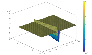
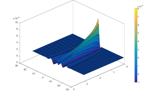
Figure 8. Lider function (left) and state (right). $T=3s,N=100,\Delta t=2\times 10^{-2}$, $\ell=\gamma=40$. Domains $\omega=(-3,1)$ and $\mathcal{O}=(2,5)$, initial datum $u_{0}(x)=10^{-3}\exp{(-x^{2})}$.

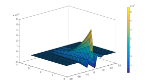
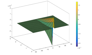
Figure 9. Disturbance (left) function and follower (right). $T=3s,N=100,\Delta t=2\times 10^{-2}$, $\ell=\gamma=40$. Domains $\omega=(-3,1)$ and $\mathcal{O}=(2,5)$, initial datum $u_{0}(x)=10^{-3}\exp{(-x^{2})}$.

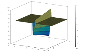
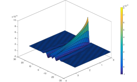
Figure 10. Lider (left) and state (right). $T=3s,N=100,\Delta t=2\times 10^{-2}$, $\ell=\gamma=40$. Domains $\omega=(-3,1)$ and $\mathcal{O}=(-1,3)$, initial datum $u_{0}(x)=10^{-3}\exp{(-x^{2})}$.

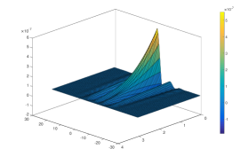
Figure 11. Disturbance function (left) and follower (right). $T=3s,N=100,\Delta t=2\times 10^{-2}$, $\ell=\gamma=40$. Domains $\omega=(-3,1)$ and $\mathcal{O}=(-1,3)$, initial datum $u_{0}(x)=10^{-3}\exp{(-x^{2})}$.

4. Comments and open problems

In this paper, we have considered the robust Stackelberg controllability problem for the KS equations. However, there are several comments and open questions that are worth mentioning.

• The robustness of a nonlinear KS equation posed in a bounded domain is achieved by using optimal control theory that allows us to guarantee the existence, uniqueness and also characterization of a saddle point for the system (1.6).

  To our knowledge, this paper contains the first numerical description concerning the robustness process for the KS equation. Due to the high–order in space (i.e., fourth order derivates), an appropriate change of variable is used to implement low–order finite elements, more precisely, $\mathbb{P}_{1}$–type Lagrange elements, meanwhile, a $\theta$–scheme/Bashforth method was used for the time discretization. Although this paper does not present an exhaustive numerical analysis of our method, since it is far way of the main goals, several configurations to the time–space discretization displayed good results for the error in the $L^{2}$–norm and $L^{\infty}$–norm, see Table 1. Besides, from the algorithms presented in [6, 39] for the Navier–Stokes system, we proposed new iterative schemes of constructing the ascent and descent directions.

• In this paper we present the robust stackelberg controllability (RSC) problem for the KS equation, that is, once we have obtained the robust pair $(\bar{v},\bar{\psi})$, we proved the exact controllability to the trajectories for the leader control $h$. A direct consequence is the Stackelberg strategy between the leader $h$ and the follower $v$. From a theoretical perspective, the main novelties are new Carleman inequalities and its relationship with the robustness parameters $\ell$ and $\gamma$, see Proposition 3.1 and Proposition 3.5.

  Numerically, some approximate solutions to the RSC problem are presented by implementing the algorithm 2. In addition, by considering the geometrical condition between the leader and the follower, i.e., $\omega\cap\mathcal{O}=\emptyset$, the numerical examples allow us to visualize that such an condition (sufficient condition in Theorem 1.2) could be removed in some sense, that means, $\omega\cap\mathcal{O}\neq\emptyset$ could proceed by using perhaps another strategy.

• It would be interesting to study the case of a cooperative game between the leader control $h$ and the follower control $v$, that is, to analyze the case in which

  $$(\mbox{leader domain }h\,\,\cap\,\,\mbox{follower control }v)\neq\emptyset.$$

• Another problem consists in the possibility of extending the notion of a robust control to several inputs, for example, instead of a control $v$ and a disturbance $\psi$, to take several control $v_{1},\cdots,v_{N}$ and several disturbance signals $\psi_{1},\cdots,\psi_{M}$, $M,N\in\mathbb{N}$.

• In the same spirit of this paper, the extension of our main results (Theorem 1.1 and Theorem 1.2) to its model in higher dimensional, that is, biharmonic–type equations could be interesting.

• Finally, efficient numerical schemes always presenting a challenge to overcome in each problem.

5. Appendix

In this appendix we mention the well–posedness results we used in this paper for both linearized and nonlinear equations. First, in order to consider external sources with lower regularity in space, we define solution by transposition for the linearized KS equation. Let us define

$$\mathcal{Z}:=C([0,T];H_{0}^{2}(0,1))\cap L^{2}(0,T;H^{4}(0,1))\cap L^{\infty}(0,T;W^{1,\infty}(0,1)).$$

Hence, let $\overline{y}_{0}\in H_{0}^{2}(0,1)$ and let $\overline{y}\in\mathcal{Z}$ be a solution of the KS equation

$$\begin{cases}\overline{y}_{t}+\overline{y}_{xxxx}+\overline{y}_{xx}+\overline{y}\overline{y}_{x}=0&\text{in }Q,\\ \overline{y}(0,t)=\overline{y}(1,t)=\overline{y}_{x}(0,t)=\overline{y}_{x}(1,t)=0&\text{on }(0,T),\\ \overline{y}(\cdot,0)=\overline{y}_{0}&\text{in }(0,1).\end{cases}$$ (5.1)

First, we consider the following linearized system:

$$\begin{cases}y_{t}+y_{xxxx}+y_{xx}+\overline{y}y_{x}+\overline{y}_{x}y=f&\text{in }Q,\\ y(0,t)=y(1,t)=y_{x}(0,t)=y_{x}(1,t)=0&\text{on }(0,T),\\ y(\cdot,0)=y_{0}&\text{in }(0,1).\end{cases}$$ (5.2)

Now, from [8, Section 2] we have the following definition.

Definition 5.1.

Let $y_{0}\in H^{-2}_{0}(0,1)$ and $f\in L^{1}(0,T;W^{-1,1}(0,1))$. A solution of the system (5.2) is a solution $y\in L^{2}(Q)$ such that for any $g\in L^{2}(Q)$,

$$\iint\limits_{Q}y(x,t)g(x,t)dxdt=\langle y_{0},w(0,\cdot)\rangle_{H^{-2}(0,1),H^{2}(0,1)}+\langle f,w\rangle_{L^{1}(0,T;W^{-1,1}(0,1)),L^{\infty}(0,T;W^{1,\infty}(0,1))},$$ (5.3)

where $w=w(x,t)\in\mathcal{Z}$ is the solution to

$$\begin{cases}-w_{t}+w_{xxxx}+w_{xx}-\overline{y}w_{x}=g&\text{in }Q,\\ w(0,t)=w(1,t)=w_{x}(0,t)=w_{x}(1,t)=0&\text{on }(0,T),\\ w(\cdot,T)=0&\text{in }(0,1).\end{cases}$$ (5.4)

Lemma 5.2.

Assume $\overline{y}\in\mathcal{Z}$. Then, for any $y_{0}\in H^{-2}_{0}(0,1)$ and $f\in L^{1}(0,T;W^{-1,1}(0,1))$, the linearized system (5.2) admits a unique solution $y\in C([0,T];H^{-2}(0,1))\cap L^{2}(0,T;L^{2}(0,1))$.

Remark 5.3.

Note that both the regularity for the solution $w$ of (5.4) and an exhaustive proof of Lemma 5.2 can be obtained in an easy way from [8, Proposition 2.1] and [22]. Due to that, we have omitted those details here.

The following lemma shows regularity results for (5.2) by considering data $(f,y_{0})$ belong to more regular spaces like $L^{2}(Q)\times L^{2}(0,1)$ and $L^{2}(Q)\times H^{2}_{0}(0,1)$. We invite to the reader to review [22] and [7, Appendix A] for more details.

Lemma 5.4.

Assume $\overline{y}\in\mathcal{Z}$.

1. For any $y_{0}\in L^{2}(0,1)$ and $f\in L^{2}(Q)$, the linearized system (5.2) admits a unique solution $y\in C([0,T];L^{2}(0,1))\cap L^{2}(0,T;H^{2}(0,1))$ with $y_{t}\in L^{2}(0,T;H^{-2}(0,1))$. Moreover, there exists a positive constant $C=C(\|\overline{y}\|_{L^{\infty}(0,T;W^{1,\infty}(0,1)).})$ such that

   $$\|y\|_{C([0,T];L^{2}(0,1))\cap L^{2}(0,T;H^{2}(0,1))}\leq C\Bigl{(}\|f\|_{L^{2}(Q)}+\|y_{0}\|_{L^{2}_{0}(0,1)}\Bigr{)}.$$ (5.5)

2. For $(y_{0},f)\in H_{0}^{2}(0,1)\times L^{2}(Q)$, the linearized system (5.2) admits a unique solution $y$ in $C([0,T];H_{0}^{2}(0,1))\cap L^{2}(0,T;H^{4}(0,1))$. Moreover,

   $$\|y\|_{C([0,T];H_{0}^{2}(0,1))\cap L^{2}(0,T;H^{4}(0,1))}\leq C\Bigl{(}\|f\|_{L^{2}(Q)}+\|y_{0}\|_{H^{2}_{0}(0,1)}\Bigr{)},$$ (5.6)

   where $C$ is a positive constant depending on $\|\overline{y}\|_{L^{\infty}(0,T;W^{1,\infty}(0,1)).}$

Now, we mention a result for coupled fourth–order system. Its proof can be found in [7, Appendix A]. Let us consider the system:

$$\begin{cases}y_{t}+y_{xxxx}+y_{xx}+\overline{y}y_{x}+\overline{y}_{x}y=g_{1}+-\mu^{-2}z&\text{in }Q,\\ -z_{t}+z_{xxxx}+z_{xx}-(y+\overline{y})z_{x}=g_{2}&\text{in }Q,\\ y(0,t)=y(1,t)=z(0,t)=z(1,t)=0&\text{on }(0,T),\\ y_{x}(0,t)=y_{x}(1,t)=z_{x}(0,t)=z_{x}(1,t)=0&\text{on }(0,T),\\ y(\cdot,0)=y_{0}(\cdot),\,\,z(\cdot,T)=0&\text{in }(0,1).\end{cases}$$ (5.7)

Lemma 5.5.

Assume that $\overline{y}\in L^{\infty}(Q)$. Then, there exists $\mu_{0}>0$ such that for every $\mu\geq\mu_{0}$, any $g_{1},g_{2}\in L^{2}(Q)$ and any $y_{0}\in L^{2}(0,1)$, $(y,z)$ is the unique solution of (5.7) in the space

$$(y,z)\in(L^{\infty}(0,T;L^{2}(0,1))\cap L^{2}(0,T;H^{2}(0,1)))^{2}.$$

The next step in this appendix corresponds to the nonlinear problem

$$\begin{cases}y_{t}+y_{xxxx}+y_{xx}+\overline{y}y_{x}+\overline{y}_{x}y+yy_{x}=f&\text{in }Q,\\ y(0,t)=y(1,t)=y_{x}(0,t)=y_{x}(1,t)=0&\text{on }(0,T),\\ y(\cdot,0)=y_{0}&\text{in }(0,1).\end{cases}$$ (5.8)

Lemma 5.6.

1. Assume $\overline{y}\in L^{\infty}(0,T;W^{1,\infty}(0,1))$. There exists $\delta>0$ such that for any $(f,y_{0})\in L^{2}(Q)\times L^{2}(0,1)$ satisfying

   $$\|y_{0}\|_{L^{2}(0,1)}+\|f\|_{L^{2}(Q)}\leq\delta$$

   problem (5.8) has a unique solution in $C([0,T];L^{2}(0,1))\cap L^{2}(0,T;H^{2}(0,1))$.

2. Let $\overline{y}=0$ in (5.8). There exists $\delta>0$ such that for any $(f,y_{0})\in L^{2}(Q)\times H_{0}^{2}(0,1)$ satisfying

   $$\|y_{0}\|_{H_{0}^{2}(0,1)}+\|f\|_{L^{2}(Q)}\leq\delta$$

   problem (5.8) has a unique solution in $C([0,T];H_{0}^{2}(0,1))\cap L^{2}(0,T;H^{4}(0,1))$.

Remark 5.7.

Although in [7, Theorem A.4] the authors have proved the first part of the above result by considering $f\in L^{1}(0,T;L^{2}(0,1))$ instead of $f\in L^{2}(0,T;L^{2}(0,1))$, their arguments can be easily adapted for proving this part of lemma 5.6. The second part can be obtained from [22]. For this reason, we have omitted the proof of Lemma 5.6.

Remark 5.8.

Observe that, from lemma 5.6, part $b)$, and the fact that $H_{0}^{2}(0,1)$ embeds continuously into $W^{1,\infty}(0,1)$, it follows that $y\in L^{\infty}(0,T;W^{1,\infty}(0,1))$.

References

- [1] Georgios D. Akrivis. Finite difference discretization of the Kuramoto-Sivashinsky equation. Numer. Math., 63(1):1–11, 1992.
- [2] Georgios D. Akrivis. Finite element discretization of the Kuramoto-Sivashinsky equation. In Numerical analysis and mathematical modelling, volume 29 of Banach Center Publ., pages 155–163. Polish Acad. Sci. Inst. Math., Warsaw, 1994.
- [3] Grégoire Allaire. Numerical analysis and optimization. Numerical Mathematics and Scientific Computation. Oxford University Press, Oxford, 2007. An introduction to mathematical modelling and numerical simulation, Translated from the French by Alan Craig.
- [4] Denis Anders, Maik Dittmann, and Kerstin Weinberg. A higher-order finite element approach to the Kuramoto-Sivashinsky equation. ZAMM Z. Angew. Math. Mech., 92(8):599–607, 2012.
- [5] Blake Barker, Mathew A. Johnson, Pascal Noble, L. Miguel Rodrigues, and Kevin Zumbrun. Nonlinear modulational stability of periodic traveling-wave solutions of the generalized Kuramoto-Sivashinsky equation. Phys. D, 258:11–46, 2013.
- [6] Thomas R. Bewley, Roger Temam, and Mohammed Ziane. A general framework for robust control in fluid mechanics. Phys. D, 138(3-4):360–392, 2000.
- [7] N. Carreño and M. C. Santos. Stackelberg–Nash exact controllability for the Kuramoto–Sivashinsky equation. J. Differential Equations, 266(9):6068–6108, 2019.
- [8] Eduardo Cerpa and Alberto Mercado. Local exact controllability to the trajectories of the 1-D Kuramoto-Sivashinsky equation. J. Differential Equations, 250(4):2024–2044, 2011.
- [9] Eduardo Cerpa, Alberto Mercado, and Ademir F. Pazoto. Null controllability of the stabilized Kuramoto-Sivashinsky system with one distributed control. SIAM J. Control Optim., 53(3):1543–1568, 2015.
- [10] PD Christofides and J Chow. Nonlinear and robust control of pde systems: Methods and applications to transport-reaction processes, 2002.
- [11] L. Jones Tarcius Doss and A. P. Nandini. A fourth-order -Galerkin mixed finite element method for Kuramoto-Sivashinsky equation. Numer. Methods Partial Differential Equations, 35(2):445–477, 2019.
- [12] Vasile Dragan, Toader Morozan, and Adrian-Mihail Stoica. Mathematical methods in robust control of linear stochastic systems, volume 50. Springer, 2006.
- [13] P. G. Drazin and R. S. Johnson. Solitons: an introduction. Cambridge Texts in Applied Mathematics. Cambridge University Press, Cambridge, 1989.
- [14] Geir E Dullerud and Fernando Paganini. A course in robust control theory: a convex approach, volume 36. Springer Science & Business Media, 2013.
- [15] Ivar Ekeland and Roger Temam. Convex analysis and variational problems. North-Holland Publishing Co., Amsterdam-Oxford; American Elsevier Publishing Co., Inc., New York, 1976. Translated from the French, Studies in Mathematics and its Applications, Vol. 1.
- [16] A. V. Fursikov and O. Yu. Imanuvilov. Controllability of evolution equations, volume 34 of Lecture Notes Series. Seoul National University, Research Institute of Mathematics, Global Analysis Research Center, Seoul, 1996.
- [17] Roland Glowinski, Jacques-Louis Lions, and Jiwen He. Exact and approximate controllability for distributed parameter systems, volume 117 of Encyclopedia of Mathematics and its Applications. Cambridge University Press, Cambridge, 2008. A numerical approach.
- [18] Michael Green and David JN Limebeer. Linear robust control. Courier Corporation, 2012.
- [19] Richard S. Hamilton. The inverse function theorem of Nash and Moser. Bull. Amer. Math. Soc. (N.S.), 7(1):65–222, 1982.
- [20] Víctor Hernández-Santamaría and Luz de Teresa. Robust Stackelberg controllability for linear and semilinear heat equations. Evol. Equ. Control Theory, 7(2):247–273, 2018.
- [21] Víctor Hernández-Santamaría and Liliana Peralta. Some remarks on the robust Stackelberg controllability for the heat equation with controls on the boundary. Discrete Contin. Dyn. Syst. Ser. B, 25(1):161–190, 2020.
- [22] Changbing Hu and Roger Temam. Robust boundary control for the Kuramoto-Sivashinsky equation. In Optimal control and partial differential equations, pages 353–362. IOS, Amsterdam, 2001.
- [23] Changbing Hu and Roger Temam. Robust control of the Kuramoto-Sivashinsky equation. Dyn. Contin. Discrete Impuls. Syst. Ser. B Appl. Algorithms, 8(3):315–338, 2001.
- [24] Yoshiki Kuramoto and Toshio Tsuzuki. On the formation of dissipative structures in reaction–diffusion systems: Reductive perturbation approach. Progress of Theoretical Physics, 54(3):687–699, 1975.
- [25] Yoshiki Kuramoto and Toshio Tsuzuki. Persistent propagation of concentration waves in dissipative media far from thermal equilibrium. Progress of theoretical physics, 55(2):356–369, 1976.
- [26] Mehrdad Lakestani and Mehdi Dehghan. Numerical solutions of the generalized Kuramoto-Sivashinsky equation using B-spline functions. Appl. Math. Model., 36(2):605–617, 2012.
- [27] Yiming Lou and Panagiotis D Christofides. Optimal actuator/sensor placement for nonlinear control of the kuramoto-sivashinsky equation. IEEE Transactions on Control Systems Technology, 11(5):737–745, 2003.
- [28] Brigitte Lucquin and Olivier Pironneau. Introduction to scientific computing. John Wiley & Sons, Ltd., Chichester, 1998. Translated from the French by Michel Kern.
- [29] D. M. Michelson and G. I. Sivashinsky. Nonlinear analysis of hydrodynamic instability in laminar flames. II. Numerical experiments. Acta Astronaut., 4(11-12):1207–1221, 1977.
- [30] R. K. Mohanty and Deepti Kaur. Numerov type variable mesh approximations for 1D unsteady quasi-linear biharmonic problem: application to Kuramoto-Sivashinsky equation. Numer. Algorithms, 74(2):427–459, 2017.
- [31] R. K. Mohanty and Deepti Kaur. High accuracy two-level implicit compact difference scheme for 1D unsteady biharmonic problem of first kind: application to the generalized Kuramoto-Sivashinsky equation. J. Difference Equ. Appl., 25(2):243–261, 2019.
- [32] Cristhian Montoya and Luz de Teresa. Robust Stackelberg controllability for the Navier-Stokes equations. NoDEA Nonlinear Differential Equations Appl., 25(5):Art. 46, 33, 2018.
- [33] H-G Purwins, HU Bödeker, and Sh Amiranashvili. Dissipative solitons. Advances in Physics, 59(5):485–701, 2010.
- [34] Alfio Quarteroni and Alberto Valli. Numerical approximation of partial differential equations, volume 23 of Springer Series in Computational Mathematics. Springer-Verlag, Berlin, 1994.
- [35] Rathinasamy Sakthivel and Hiroshi Ito. Non-linear robust boundary control of the Kuramoto-Sivashinsky equation. IMA J. Math. Control Inform., 24(1):47–55, 2007.
- [36] Brajesh Kumar Singh, Geeta Arora, and Pramod Kumar. A note on solving the fourth-order kuramoto-sivashinsky equation by the compact finite difference scheme. Ain Shams Engineering Journal, 2016.
- [37] G. I. Sivashinsky. Nonlinear analysis of hydrodynamic instability in laminar flames. I. Derivation of basic equations. Acta Astronaut., 4(11-12):1177–1206, 1977.
- [38] Heinrich von Stackelberg et al. Theory of the market economy. 1952.
- [39] T. Tachim Medjo. Iterative methods for a class of robust control problems in fluid mechanics. SIAM J. Numer. Anal., 39(5):1625–1647, 2001/02.
- [40] Heinrich Von Stackelberg. Market structure and equilibrium. Springer Science & Business Media, 2010.
- [41] Yan Xu and Chi-Wang Shu. Local discontinuous Galerkin methods for the Kuramoto-Sivashinsky equations and the Ito-type coupled KdV equations. Comput. Methods Appl. Mech. Engrg., 195(25-28):3430–3447, 2006.
- [42] J Yanez and M Kuznetsov. An analysis of flame instabilities for hydrogen–air mixtures based on sivashinsky equation. Physics Letters A, 380(33):2549–2560, 2016.
- [43] Zhongcheng Zhou. Observability estimate and null controllability for one-dimensional fourth order parabolic equation. Taiwanese J. Math., 16(6):1991–2017, 2012.