Operational Entanglement of Symmetry-Protected Topological Edge States

Abstract

We use an entanglement measure that respects the superselection of particle number to study the non-local properties of symmetry-protected topological edge states. Considering half-filled $M$-leg Su-Schrieffer-Heeger (SSH) ladders as an example, we show that the topological properties and the operational entanglement extractable from the boundaries are intimately connected. Topological phases with at least two filled edge states have the potential to realize genuine, non-bipartite, many-body entanglement which can be transferred to a quantum register. The entanglement is extractable when the filled edge states are sufficiently localized on the lattice sites controlled by the users. We show, furthermore, that the onset of entanglement between the edges can be inferred from local particle number spectroscopy alone and present an experimental protocol to study the breaking of Bell’s inequality.

I Introduction

Entanglement in a quantum system is an essential resource for quantum algorithms and for quantum encryption keys. In order to use this resource, an important question is how much of the entanglement present in a quantum state is accessible and can be transfered by local operations to a quantum register consisting of distinguishable qubits. A fundamental difficulty in addressing this question for many-body states of itinerant particles is that the entangled entities itself are indistinguishable. Suppose observers, Alice and Bob, have access to two spatially-separated parts of a quantum system of indistinguishable particles with a conserved particle number N. Then there is always a local operation that will collapse the pure or mixed quantum state $\rho_{AB}$ they share into a state $\rho_{AB}^{n_{A},n_{B}}$ with fixed local particle numbers $n_{A}$ ($n_{B}$) for Alice (Bob). The operational entanglement (also called accessible entanglement or entanglement of particles) which can be transferred to a quantum register is thus given by [1, 2]

$$E_{\textrm{op}}=\sum_{n_{A},n_{B}}p(n_{A},n_{B})E[\rho_{AB}^{n_{A},n_{B}}]$$ (1)

where $p(n_{A},n_{B})=\tr\rho_{AB}^{n_{A},n_{B}}$ is the probability to project onto a state with $n_{A},n_{B}$ particles in the two subsystems and $E[\rho]$ is an entanglement measure applied to the normalized projected state. The superselection of particle number also gives rise to an additional non-local resource associated with the particle number fluctuations [3, 4]. To characterize this second, complementary resource we introduce the generalized number entropy (Shannon entropy)

$$E_{n}=-\sum_{n_{A},n_{B}}p(n_{A},n_{B})\ln p(n_{A},n_{B})\;.$$ (2)

We note that $E_{n}=0$ if $n_{A}$ and $n_{B}$ are fixed, $E_{n}$ has an upper bound $E^{\textrm{max}}_{n}=\ln[(n_{A}^{\textrm{max}}+1)(n_{B}^{\textrm{max}}+1)]$ if there are at most $n_{A}^{\textrm{max}}$ ($n_{B}^{\textrm{max}}$) particles in $A$ ($B$), and $E_{n}$ does not increase under local operations.

For a bipartition of a pure state $\rho$, one can use the von-Neumann entanglement entropy $E_{vN}$ as the entanglement measure. In this case, $E_{\textrm{vN}}=E_{n}+E_{\textrm{op}}$ where the operational or configurational entropy is now given by Eq. (1) with $E[\rho]\equiv E_{\textrm{vN}}[\rho]$ [5, 6, 7, 8, 9, 10] and the restriction $n_{B}=N-n_{A}$ is placed on the sums in Eqs. (1, 2). The number entropy for a bipartition has recently been measured in a cold atomic gas experiment [11] and can be used to obtain a bound on the total entanglement entropy [12, 13].

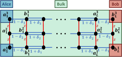
Figure 1: $3$-leg SSH ladder of spinless fermions. Along the chain direction the hopping amplitude alternates between $1-\delta_{s}$ and $1+\delta_{s}$ while $z$ is the intrachain coupling. Alice and Bob only control a few sites at opposite edges of the ladder.

Long-range entanglement in many-body systems is, in general, very fragile against local perturbations. An exception are edge states in systems with a topologically non-trivial bulk. In this case, the number of edge states is topologically protected and cannot be changed without closing the gap or breaking the symmetry [14, 15]. Since topological edge states can exist simultaneously on multiple edges, a filled edge state is a non-local quantum resource.

In this article we will show that symmetry-protected topological edge states in lattice models can be a source of genuine, spatially-separated, non-bipartite many-body entanglement which can be transfered to a quantum register. We will show, furthermore, that the onset of entanglement between the edges can be inferred from local particle number spectroscopy, making it measurable, for example, by current-day cold atomic gas experiments [11, 16, 17]. We also present an experimental protocol to test Bell’s inequalities [18, 19, 20, 21, 22]. We find that for half-filled pure states of arbitrary length, two or more filled edge states are required to break the inequality. Furthermore, using the grand canonical and canonical ensemble, we establish the spatially separated, operational breaking of Bell’s inequality of a many-body system in thermal equilibrium.

In the following, we will consider lattice models of itinerant spinless fermions. Let us first briefly discuss why in this case a single edge state is insufficient to produce any operational entanglement. Let us assume that the edge state is very sharply localized at the left and right edges of a chain which are controlled by Alice and Bob, respectively. To simplify the argument, we ignore the bulk completely for now and assume that the edge state is a single-particle pure state. A maximally entangled edge state in occupation number representation is then of the form $|\Psi\rangle=(|10\rangle\pm|01\rangle)/\sqrt{2}$ and has von-Neumann entanglement entropy $E_{\textrm{vN}}=\ln 2$. If Alice and Bob measure their local particle numbers in order to perform local operations, this state however collapses onto the product state $|\Psi^{1,0}\rangle\propto|10\rangle$ or $|\Psi^{0,1}\rangle\propto|01\rangle$. Thus, this state has only number entropy $E_{n}$ but no operational entanglement. We therefore need at least two filled edge states to have any operational entanglement. In the latter case, the projected state $|\Psi^{1,1}\rangle$ can have operational entanglement while the states $|\Psi^{2,0}\rangle$ and $|\Psi^{0,2}\rangle$ are again product states.

II Model

In order to build a system with more than one filled edge state at half-filling, we couple Su-Schrieffer-Heeger (SSH) chains [23, 24] to form $M$-leg ladders. While there are many other possible choices, the SSH chain is one of the simplest systems with non-local, symmetry-protected topological edge states. Furthermore, its properties can be studied experimentally using cold atoms in optical superlattices [25, 26, 27]. Open boundary conditions can be implemented using an optical box potential [28, 29]. As we will show below, the operational entanglement that results from the topological edge states can be observed in this system using modern experimental techniques.

Let $J$, $\delta_{s}$ and $z$ be real constants that indicate hopping between sites, and ${a_{j}^{s}}^{\dagger}$ (${b_{j}^{s}}^{\dagger}$) creation operators of an ‘a’ (‘b’) spinless fermion on chain $s$, in unit cell $j$. The unit cell consists of $2M$ elements, two elements on each of the $M$ chains. The Hamiltonian of the model in second quantization is then given by

$$H = J\sum_{j,s}\{(1-\delta_{s}){a_{j}^{s}}^{{\dagger}}b_{j}^{s}+(1+\delta_{s}){b_{j}^{s}}^{{\dagger}}a_{j+1}^{s}+h.c.\}$$ (3)

$$+ z\sum_{j,s}\{{a_{j}^{s}}^{{\dagger}}a_{j}^{s+1}+{b_{j}^{s}}^{{\dagger}}b_{j}^{s+1}+h.c.\}$$

with $J=1$ and $|\delta_{s}|\leq 1$ for the remainder of the paper. A visualization of the SSH ladder for $M=3$ with open boundary conditions is shown in Fig. 1.

The non-interacting SSH ladder, a member of the BDI symmetry class, has three non-spatial symmetries. These symmetries are time reversal $\hat{T}$, charge-conjugation $\hat{C}$, and chiral $\hat{S}$, see Ref. [15]. The relevant symmetry here is the chiral symmetry. $\hat{S}$ is defined in terms of its action on annihilation operators as

$$\hat{S}a_{j}^{s}\hat{S}^{-1}=(-1)^{s+1}{a_{j}^{s}}^{\dagger},\ \hat{S}b_{j}^{s}\hat{S}^{-1}=(-1)^{s}{b_{j}^{s}}^{\dagger},$$ (4)

with $\hat{S}i\hat{S}^{-1}=-i$. The Hamiltonian in Eq. (3) satisfies the symmetries $\hat{T}H\hat{T}^{-1}=H$, $\hat{C}H\hat{C}^{-1}=H$, and $\hat{S}H\hat{S}^{-1}=H$ for any values of $J$, $\delta_{s}$ and $z$. There are also additional non-spatial symmetries present when certain restrictions are placed on the parameters. In particular, additional chiral symmetries enable additional topological invariants [30] which are discussed further in App. C.

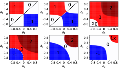
Figure 2: Topological phase diagram for $M=2$ and $M=3$ leg ladders. The numbers indicate the value of the topological invariant $I$. A dotted line or an ’x’ is placed where the analytical result, Eq. (6), applies. Top, left to right: $M=2$, $z=0.0$; $M=2$, $z=0.4$; $M=3$, $z=0.9$, $\delta_{2}=-0.75$. Bottom, left to right: $M=3$, $z=0.9$, $\delta_{2}=-0.25$; $M=3$, $z=0.9$, $\delta_{2}=0.25$; $M=3$, $z=0.9$, $\delta_{2}=0.75$.

III Topology

In order to find the number of edge states of the $M$-leg SSH ladder for a given set of parameters, we have to analyze its topological phase diagram. To define the winding number $I$ for our system with chiral symmetry, we follow Ref. [31].

First, we define a unitary matrix $U_{S}$ for the chiral symmetry $\hat{S}$ from the condition $\hat{S}\psi_{n}\hat{S}^{-1}=\sum_{m}(U_{S})_{n,m}^{*}\psi_{m}^{\dagger}$, where $\psi_{n}$ are the $a_{j}^{s}$ and $b_{j}^{s}$ operators in an arbitrary basis. $U_{S}$ has the property $\mbox{tr}\,U_{S}=0$ and we define the phase such that $U_{S}^{2}=\mathbb{I}$. $U_{S}$ can be put into a momentum space, block diagonal form represented by $U_{S}(k)$. Let $g(k)=H^{-1}(k)$ be the matrix representation of the single particle Green’s function corresponding to the Hamiltonian $H$ in Eq. (3). Then the topological invariant is given by [31, 30, 32]

$$I=\frac{1}{4\pi\text{i}}\mbox{tr}\int dk\ {U_{S}}(k)g^{-1}(k)\partial_{k}g(k),$$ (5)

which, for non-interacting systems, is equivalent to the winding number as defined, for example, in Ref. [15]. We prove the equivalence of the invariants in App. A. We note, furthermore, that the related Zak phase for a single SSH chain has been measured experimentally in cold atomic gases [25]. Before analyzing the full topological phase diagram for $M=2$ and $M=3$ leg ladders numerically, we first note the following important analytical result for the general $M$-leg case: Suppose that $\delta_{1}=\delta_{2}=\dots\equiv\delta$ and $0\leq|z|\cos(\frac{\pi}{M+1})<|\delta|$. (i) If $\delta<0$, then $I=0$. (ii) If $\delta>0$, then

$$I=1\quad\mbox{for $M$ odd,}\;\;\mbox{and}\quad I=0\quad\mbox{for $M$ even.}$$ (6)

The proof of this result can be found in App. B. We note that this even-odd effect resembles the celebrated result for spin-$1/2$ ladders [33].

The topological phase diagram based on the invariant defined in Eq. (5) is presented in Fig. 2 for ladders with $M=2$ and $M=3$. A dotted line or an ’x’ is placed where the analytical result, Eq. (6), applies. A similar phase diagram for the $M=2$ case using a different parameterization can be found in Ref. [32]. When $I=0$ we have no edge states and when $I=\pm 1$ we have a single filled edge state. The case which we want to concentrate on in the following is $I=2$ where we have two filled edge states.

IV Entanglement

The ground state of the SSH ladder is described by a pure state wave function $\rho=|\Psi\rangle\langle\Psi|$. We imagine however, that Alice and Bob have access to only a small number of sites at the edges of the system. Note that in contrast to the often studied case of a bipartition, tracing out the rest of the system leads to a mixed state $\rho_{AB}$ which is our starting point.

Now that we have a density matrix $\rho_{AB}$ that only describes the two subsystems we are interested in, we can apply the operational entanglement measure defined in Eq. (1) with $E[\rho]$ being a bipartite measure of entanglement for a mixed state. Regardless of the chosen mixed state measure of entanglement, $E_{\textrm{op}}$ is not easy to compute in general. However, for small dimensions of $\rho_{AB}$ a calculation of its matrix elements using correlation functions is feasible [2]. For the case of two edge states ($I=2$) considered here the only projected density matrix which will contribute to $E_{\textrm{op}}$ is $\rho_{AB}^{1,1}$. We will call the two modes on one side of the ladder $A_{1}$ and $A_{2}$, and the modes on the other side $B_{1}$ and $B_{2}$. Next, we define the projection operators $P^{A}=A_{1}^{\dagger}A_{1}(1-A_{2}^{\dagger}A_{2})+(1-A_{1}^{\dagger}A_{1})A_{2}^{\dagger}A_{2}$ and analoguously $P^{B}$ which project the ground state onto a (non-normalized) state with a single particle in each subsystem, $|\Psi^{1,1}\rangle=P^{A}P^{B}|\Psi\rangle$. The matrix elements of the $4\times 4$ matrix $\rho_{AB}^{1,1}$ can now be computed from correlation functions in the projected state,

$$(\rho_{AB}^{1,1})_{ii^{\prime}}^{jj^{\prime}} = \tr_{A,B}(\rho_{AB}^{1,1}A_{j}^{\dagger}B_{j^{\prime}}^{\dagger}{B_{i^{\prime}}}A_{i})$$ (7)

$$= \langle\Psi^{1,1}|A_{j}^{\dagger}B_{j^{\prime}}^{\dagger}{B_{i^{\prime}}}A_{i}|\Psi^{1,1}\rangle.$$

A more detailed description of how to calculate the matrix elements of $\rho_{AB}^{1,1}$ is given in App. D. In systems—such as the SSH ladder considered here—which are Gaussian, we can use Wick’s Theorem to turn the multi-point correlation functions into products of two-point correlation functions. Since we already know from the topological phase diagram, Fig. 2, that we need at least a $3$-leg ladder to have two filled edge states, we concentrate on this case in the following. The choice of the few sites controlled by Alice and Bob needs to be based on prior knowledge of where the topological edge states are primarily located. Based on numerical results for strong dimerizations, we choose $A_{1}=a_{1}^{1}$, $A_{2}=a_{1}^{3}$, $B_{1}=b_{L}^{1}$ and $B_{2}=b_{L}^{3}$, see Fig. 1.

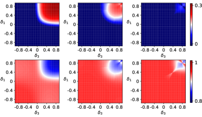
Figure 3: Entanglement phase diagram based on $E_{\textrm{op}}=p(1,1)E_{\textrm{neg}}[\rho_{AB}^{1,1}]$ in units of $\ln 2$ and generalized number entropy $E_{n}$ in units of $\ln 9$ for $3$-leg ladders with $L=16$. Results for $E_{\textrm{op}}$ are shown in the top panels and for $E_{n}$ in the bottom panels. Left to right: $z=0.9$, $\delta_{2}=-0.75$; $z=0.9$, $\delta_{2}=-0.25$; $z=0.9$, $\delta_{2}=0.25$.

There are many different entanglement measures one can use to quantify the entanglement of a mixed-state density matrix [34]. Here we use an additive measure of entanglement, the logarithmic negativity [35, 36],

$$E_{\textrm{neg}}[\rho_{AB}]=\ln(||\rho_{AB}^{T_{A}}||)\,,$$ (8)

where $\rho_{AB}^{T_{A}}$ is the partial transpose with respect to Alice and $||\rho_{AB}^{T_{A}}||$ is the trace norm of the normalized matrix. Results for $E_{\textrm{op}}=p(1,1)E_{\textrm{neg}}[\rho_{AB}^{1,1}]$ for the $3$-leg ladder—using the same dimerizations $\delta_{s}$ as in the topological phase diagrams—are shown in Fig. 3. For $\delta_{2}=-0.75$ and $\delta_{2}=-0.25$, the regions where $E_{\textrm{neg}}[\rho_{AB}^{1,1}]\approx\ln 2$ coincide with the regions in Fig. 2 with winding number $I=2$. The topology of the system is thus directly tied to the operational entanglement which can be extracted from the system by Alice and Bob. However for $\delta_{2}=0.25$, the region with operational entanglement is much smaller than the region with $I=2$. In this case, the edge states are not sufficiently localized. Alice and Bob would need to control more sites to extract all of the operational entanglement present in the two edge states. Virtually identical results are obtained if we use the entanglement of formation instead of the logarithmic negativity, see App. E. From an experimental perspective, the most important result however is that the regions with operational entanglement and winding number $I=2$ can be identified by simply measuring the generalized number entropy $E_{n}$, Eq. (2), on a small number of sites only, see bottom panels in Fig. 3. When the edge states are forming, $p(n_{A}=1,n_{B}=1)$ increases leading to a decrease of $E_{n}$. The number entropy can be measured straightforwardly in cold atomic gases by single-site atomic imaging as has recently been demonstrated in Ref. [11].

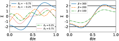
Figure 4: $\Sigma$, as defined in Eq. (9), for a $3$-leg ladder. Left panel: $T=0$ with $L=16$, $\delta_{1}=0.9$, $\delta_{3}=0.8$, and $z=0.9$ for different $\delta_{2}$. For $\delta_{2}=-0.75$, corresponding to a winding number $I=2$, the CHSH inequality is broken. Right panel: $L=8$, $\delta_{1}=0.29$, $\delta_{2}=-0.99$, $\delta_{3}=0.99$, $z=0.95$ and chemical potential $\mu=0$ for various inverse temperatures $\beta=1/T$.

V Bell’s theorem

Moving beyond the indirect observation of the entanglement between the edges by monitoring the number entropy, one of the most fundamental ways to prove that two qubits are entangled is to show that a Bell inequality is broken. Here we will choose the Clauser, Horne, Shimony and Holt (CHSH) [20, 22] version of Bell’s inequality. Let $\boldsymbol{a}$, $\boldsymbol{a}^{\prime}$, $\boldsymbol{b}$, and $\boldsymbol{b}^{\prime}$ be three-dimensional vectors. Let $\boldsymbol{\sigma}^{A/B}$ be the vector of $A/B$ Pauli matrices. Defining $\langle\dots\rangle_{1,1}=tr(\rho_{AB}^{1,1}\dots)/p(1,1)$, the CHSH inequality reads

$$-2\leq\Sigma_{\boldsymbol{a},\boldsymbol{a}^{\prime},\boldsymbol{b},\boldsymbol{b}^{\prime}}\leq 2\,,\qquad\mbox{with}$$ (9)

$$\Sigma_{\boldsymbol{a},\boldsymbol{a}^{\prime},\boldsymbol{b},\boldsymbol{b}^{\prime}}=\langle(\boldsymbol{a}\cdot\boldsymbol{\sigma}^{A})(\boldsymbol{b}\cdot\boldsymbol{\sigma}^{B})\rangle_{1,1}-\langle(\boldsymbol{a}^{\prime}\cdot\boldsymbol{\sigma}^{A})(\boldsymbol{b}\cdot\boldsymbol{\sigma}^{B})\rangle_{1,1}$$

$$+\langle(\boldsymbol{a}\cdot\boldsymbol{\sigma}^{A})(\boldsymbol{b}^{\prime}\cdot\boldsymbol{\sigma}^{B})\rangle_{1,1}+\langle(\boldsymbol{a}^{\prime}\cdot\boldsymbol{\sigma}^{A})(\boldsymbol{b}^{\prime}\cdot\boldsymbol{\sigma}^{B})\rangle_{1,1}.$$

To show the breaking of the inequality, we choose the vectors $\boldsymbol{a}$, $\boldsymbol{a}^{\prime}$, $\boldsymbol{b}$ and $\boldsymbol{b}^{\prime}$ to be in the x-z plane with $\boldsymbol{a}\cdot\boldsymbol{\sigma}^{A}=\cos\theta_{a}\sigma_{z}^{A}+\sin\theta_{a}\sigma_{x}^{A}$ and $\boldsymbol{b}\cdot\boldsymbol{\sigma}^{B}=\cos\theta_{b}\sigma_{z}^{B}+\sin\theta_{b}\sigma_{x}^{B}$. We use the representation of the Pauli operators $\sigma_{x}^{A}=A_{1}^{\dagger}A_{2}+A_{2}^{\dagger}A_{1}$, $\sigma_{y}^{A}=-iA_{1}^{\dagger}A_{2}+iA_{2}^{\dagger}A_{1}$, $\sigma_{z}^{A}=A_{1}^{\dagger}A_{1}-A_{2}^{\dagger}A_{2}$ and similarly for $\sigma_{x,y,z}^{B}$. Results for the $3$-leg ladder are shown in Fig. 4 with $\theta\equiv\theta_{a}=\theta_{b^{\prime}}/2=\theta_{a^{\prime}}/3$ and $\theta_{b}=0$. For $\delta_{2}=-0.75$, corresponding to a winding number $I=2$ (see top right panel in Fig. 2), the CHSH inequality in the projected state $\rho_{AB}^{1,1}$ is broken. Note that while $\delta_{2}=-0.25$ and $\delta_{2}=0.25$ also correspond to $I=2$, the edge states are not sufficiently localized in these cases to break the CHSH inequality.

We can also evaluate the correlators in the system in thermal equilibrium for the grand canonical and canonical ensembles. At zero temperature, there are two filled edge states and two empty edge states. The energy gap between the filled and empty edge states decreases as the system size is increased. At finite temperature, this energy gap is directly related to the filling of the four edge states. In the grand canonical case, we require the chemical potential $\mu=0$ in order to maintain particle-hole symmetry. The right panel of Fig. 4 shows that for the grand canonical ensemble, the CHSH inequality is broken for temperatures up to $\beta=1/T\approx 200$. The canonical case is discussed in App. F.

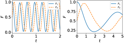
Figure 5: Fidelities (11) showing that the time evolution with the Hamiltonian (10) leads to an effective rotation of the density matrix by $\pi/2$ around the $y$-axis. When $\kappa=10$ (left), there is a nearly perfect rotation. $\kappa=1$ (right) does not result in a purely rotational process. Both figures have parameters $M=3$, $L=16$, $\delta_{1}=0.9$, $\delta_{2}=-0.75$, $\delta_{3}=0.8$ and $z=0.9$.

VI Experimental protocol

Next, we discuss a possible experimental protocol for showing that Bell’s inequality is broken. We can relate elements $\langle\sigma_{A}^{x,z}\sigma_{B}^{x,z}\rangle_{1,1}$ to two-particle correlators of the full many-body state $|\psi\rangle$. Calculating $\langle\sigma_{A}^{z}\sigma_{B}^{z}\rangle_{1,1}$ then amounts to calculating density-density correlations which are experimentally accessible [37]. A function such as $\langle\sigma_{A}^{z}\sigma_{B}^{x}\rangle_{1,1}$, on the other hand, is more difficult to obtain experimentally because it involves measuring correlators such as $\langle A_{1}^{\dagger}A_{1}B_{1}^{\dagger}B_{2}\rangle$, see App. D.

While for non-interacting systems measuring the single-particle correlation functions might be possible and is sufficient, we can more generally make use of the matrix operation $\sigma^{z}\otimes\sigma^{x}=(I\otimes R)(\sigma^{z}\otimes\sigma^{z})(I\otimes R^{\dagger})$, where $R$ is a $\pi/2$ rotation matrix about the $y$-axis and $I$ the identity matrix. In the following, we show that by time evolving the full many-body state $|\psi\rangle$, we can implement a rotation operator $R$ on the two-site density matrix $\rho_{AB}^{1,1}$. To do so, we use the time evolution operator $\exp(-\text{i}H^{\prime}t)$ with

$$H^{\prime}=H+\lambda B_{1}^{\dagger}B_{2}+\lambda^{*}B_{2}^{\dagger}B_{1},$$ (10)

$H$ defined in Eq. (3), and $\lambda$ a constant. We now compare the two-site rotated density matrix $(I\otimes R)\rho_{AB}^{1,1}(I\otimes R^{\dagger})$ with the two-site density matrix $\sigma_{AB}^{1,1}(t)$ obtained from the full time-evolved state $|\Psi(t)\rangle$ using the fidelity function for density matrices [38, 39, 40, 41]

$$F(\rho,\sigma)=\left[\ \tr\sqrt{\sqrt{\sigma}\rho\sqrt{\sigma}}\ \right]^{2}.$$ (11)

Since we want to rotate around the $y$-axis, we set $\lambda=-i\kappa$ with $\kappa$ being a real number. We define $F_{1}(t)=F(\rho_{AB}^{1,1},\sigma_{AB}^{1,1})$ and $F_{2}(t)=F((I\otimes R)\rho_{AB}^{1,1}(I\otimes R^{\dagger}),\sigma_{AB}^{1,1})$ with $F_{1}(0)=1$ and $F_{2}(0)=0.5$. The time dependence of $F_{1}$ and $F_{2}$ is shown in Fig. 5. For large $\kappa\sim 10$, $F_{1}$ and $F_{2}$ oscillate out of phase with a maximum fidelity close to $1$. This shows that implementing the coupling (10) allows for an effective rotation of the density matrix.

VII Conclusions

We have shown that symmetry-protected topological edge states in a system of itinerant particles can be a resource of spatially separated, non-bipartite, operational entanglement which can be transfered to a quantum register of distinguishable qubits. Two edge states which are both filled and sufficiently localized are required to obtain two entangled qubits. While we have used an explicit construction of such edge states based on coupled SSH chains, the connection established here between the topology of the system and the amount of entanglement which can be extracted from its edge states is expected to be general. We have shown, furthermore, that the number entropy measured on a few sites only is an indirect probe of the topological and entanglement properties of a system, which is easily accessible in cold atomic gas experiments. Going one step further, we have also demonstrated that the non-bipartite operational entanglement obtained from the projected ground state of the many-body system is sufficient to break Bell’s inequality and presented a protocol to measure these strong, spatially separated quantum correlations experimentally.

Appendix A Equivalence of Topological Invariants

We will manipulate

$$I=\frac{1}{4\pi\text{i}}\mbox{tr}\int dk\ {U_{S}}(k)g^{-1}(k)\partial_{k}g(k)$$ (A.1)

with $g(k)=H^{-1}(k)$ into an equivalent form. We first note that $U_{S}$ can be put into block diagonal form in momentum space with the blocks represented by $U_{S}(k)$. The property $U_{S}^{2}=\mathbb{I}$ for the full matrix implies a similar property of the blocks $U_{S}^{2}(k)=\mathbb{I}_{2M}$ where $M$ is the number of legs of the SSH ladder. Also since $\hat{S}$ is a non-spatial symmetry, $\text{tr}\,U_{s}=0$ implies that $\text{tr}\,U_{s}(k)=0$ for the individual blocks as well. Then $U_{S}^{2}(k)=\mathbb{I}_{2M}$ and $\text{tr}\,U_{S}(k)=0$ imply that we can pick a basis such that

$$U_{S}(k)=\begin{pmatrix}\mathbb{I}_{M}&0\\ 0&-\mathbb{I}_{M}\end{pmatrix}.$$ (A.2)

The operator condition $\hat{S}H\hat{S}^{-1}=H$ implies for the momentum blocks that $U_{S}^{\dagger}(k)H(k)U_{S}(k)=-H(k)$. This condition implies that in the same basis as (A.2),

$$H(k)=\begin{pmatrix}0&D(k)\\ D^{\dagger}(k)&0\end{pmatrix}.$$ (A.3)

Then plugging (A.2) and (A.3) into (A.1), we get

$$I=\frac{1}{4\pi i}tr\int dk\ \{D\partial_{k}D^{-1}-D^{\dagger}\partial_{k}{D^{\dagger}}^{-1}\}.$$ (A.4)

Now, we use the polar decomposition $D(k)=|D(k)|q(k)$, where $|D(k)|$ is positive definite and $q(k)$ is unitary. We obtain

$$I=\frac{\text{i}}{2\pi}\mbox{tr}\int dk\ q^{\dagger}(k)\partial_{k}q(k).$$ (A.5)

Now we demonstrate that this method of finding the topological invariant is equivalent to the method based on projection operators [14, 15]. The formalism starts by writing the Hamiltonian $H(k)$ in the off block diagonal basis Eq. (A.3). Next, we find the column eigenvectors $v_{n}(k)$ of Eq. (A.3). We define

$$P(k)=\sum_{n}v_{n}(k)v_{n}^{\dagger}(k)$$ (A.6)

where the sum is over all eigenvectors $v_{n}(k)$ with negative eigenvalues. We also define

$$Q(k)=\mathbb{I}-2P(k).$$ (A.7)

$Q(k)$ turns out to always be of the form

$$Q(k)=\begin{pmatrix}0&\tilde{q}(k)\\ \tilde{q}^{\dagger}(k)&0\end{pmatrix}.$$ (A.8)

Then the invariant is calculated by plugging $\tilde{q}(k)$ into Eq. (A.5) as $q(k)$.

Now, we only need to prove that $\tilde{q}(k)=q(k)$. To do so, first define $u_{n}(k)$ as the normalized eigenvectors of $|D(k)|$. Then the eigenvectors $v_{n}(k)$ with negative eigenvalues are

$$v_{n}(k)=\frac{1}{\sqrt{2}}\begin{pmatrix}u_{n}(k)\\ -q^{\dagger}(k)u_{n}(k)\end{pmatrix}.$$ (A.9)

Next, we use Eq. (A.9) as the vectors in Eq. (A.6) to obtain the projection operators $P(k)$ and $Q(k)$. We will also use the fact that the $u_{n}(k)$ vectors form a complete basis. We obtain

$$Q(k)=\begin{pmatrix}0&q(k)\\ q^{\dagger}(k)&0\end{pmatrix}.$$ (A.10)

Hence $\tilde{q}(k)=q(k)$.

Appendix B Proof of the Analytic Result

Analytic Result. Suppose that $\delta_{1}=\delta_{2}=\dots\equiv\delta$ and $0\leq|z|\cos(\frac{\pi}{M+1})<|\delta|$. (i) If $\delta<0$, then $I=0$. (ii) If $\delta>0$, then

$$I=1\quad\mbox{for $M$ odd,}\;\;\mbox{and}\quad I=0\quad\mbox{for $M$ even.}$$ (B.1)

Proof. Define for all chains s

$$a_{j}^{s}=\dfrac{1}{\sqrt{L}}\sum_{n=1}^{L}e^{ik_{n}j}a_{k_{n}}^{s}\ ,\ b_{j}^{s}=\dfrac{1}{\sqrt{L}}\sum_{n=1}^{L}e^{ik_{n}j}b_{k_{n}}^{s}$$ (B.2)

where $k_{n}=2\pi n/L$ (we will denote $k_{n}$ as just $k$ going forward). If $M$ is odd, define $\hat{\psi}(k)=\begin{pmatrix}a_{k}^{1}&b_{k}^{2}&a_{k}^{3}&...&a_{k}^{M}&b_{k}^{1}&a_{k}^{2}&...&b_{k}^{M}\end{pmatrix}^{T}$ and if $M$ is even, define $\hat{\psi}(k)=\begin{pmatrix}a_{k}^{1}&b_{k}^{2}&a_{k}^{3}&...&b_{k}^{M}&b_{k}^{1}&a_{k}^{2}&...&a_{k}^{M}\end{pmatrix}^{T}$. In either case, the Hamiltonian operator $H$ can be written in terms of $2M\times 2M$ block matrices $H(k)$ as

$$H=\sum_{k}\hat{\psi}^{\dagger}(k)H(k)\hat{\psi}(k).$$ (B.3)

$H(k)$ takes the form

$$H(k)=\begin{pmatrix}0_{M}&D(k)\\ D^{\dagger}(k)&0_{M}\end{pmatrix}.$$ (B.4)

where the $D(k)$ blocks are $M\times M$ matrices. If we define $x(k)=|x(k)|e^{i\theta(k)}=(1-\delta)+(1+\delta)e^{-ik}$, $D(k)$ can be written as

$$D(k)=\begin{pmatrix}x(k)&z&0&\dots\\ z&x^{*}(k)&z&\dots\\ 0&z&x(k)&\dots\\ \vdots&\vdots&\vdots&\ddots&\end{pmatrix}.$$ (B.5)

Since the symmetry $\hat{S}$ is a non-spatial chiral symmetry, the symmetry operator in Fourier space can be found by replacing $j\rightarrow k_{n}$ in Eq. (4) of the main text. Then one applies the condition $\hat{S}\psi_{n}\hat{S}^{-1}=\sum_{m}(U^{S})_{n,m}^{*}\psi_{m}^{\dagger}$, where $\psi_{n}$ are the $a_{k_{n}}^{s}$ and $b_{k_{n}}^{s}$ operators in an arbitrary basis. In the basis of Eq. (B.4), $U_{S}(k)$ takes the form

$$U_{S}(k)=\begin{pmatrix}\mathbb{I}_{M}&0_{M}\\ 0_{M}&-\mathbb{I}_{M}\end{pmatrix}.$$ (B.6)

Define $\hat{e}_{1}$, $\hat{e}_{2}$, …$\hat{e}_{2M}$ as the unit column vectors in the same basis as (B.4). For $s=1,2,\dots,M$, define

$$v_{s}^{-}=\frac{1}{\sqrt{2}}(-C_{s}\hat{e}_{s}+\hat{e}_{s+M})$$ (B.7)

$$v_{s}^{+}=\frac{1}{\sqrt{2}}(C_{s}\hat{e}_{s}+\hat{e}_{s+M}).$$ (B.8)

with

$$C_{s}=\begin{cases}e^{i\theta}&\text{s odd}\\ e^{-i\theta}&\text{s even}.\end{cases}$$ (B.9)

Then $v_{s}^{\pm}$ are the eigenvectors of $H(k)$ when $z=0$. The eigenvalues are $E_{s}^{\pm}(k)=\pm|x(k)|$. Now we transform $H(k)$ into the $v_{s}^{\pm}$ basis. Let V be defined by the unit column vectors $v_{s}^{\pm}$ as

$$V=\begin{pmatrix}v_{1}^{-}&v_{2}^{-}&\dots&v_{M}^{-}&v_{1}^{+}&v_{2}^{+}&\dots&v_{M}^{+}\end{pmatrix}.$$ (B.10)

Then

$$V^{\dagger}H(k)V=\begin{pmatrix}H_{1,1}^{V}(k)&0_{M}\\ 0_{M}&H_{2,2}^{V}(k)\end{pmatrix}$$ (B.11)

where $H_{1,1}^{V}(k)$ and $H_{2,2}^{V}(k)$ are $M\times M$ tridiagonal matrices defined by

$$H_{2,2}^{V}=-H_{1,1}^{V}=\begin{pmatrix}|x(k)|&ze^{-i\theta(k)}&0&\dots\\ ze^{i\theta(k)}&|x(k)|&ze^{i\theta(k)}&\dots\\ 0&ze^{-i\theta(k)}&|x(k)|&\dots\\ \vdots&\vdots&\vdots&\ddots&\end{pmatrix}.$$ (B.12)

Without the phase terms, the above matrix has a well known solution for a free particle with open boundary conditions. By modifying the well known open boundary solution with phase factors, we can find the eigenpairs of $H_{2,2}^{V}(k)=-H_{1,1}^{V}(k)$ and therefore obtain the eigenvectors of $V^{\dagger}H(k)V$. The eigenpairs of $H_{2,2}^{V}(k)=-H_{1,1}^{V}(k)$ are

$$u_{s}=\sqrt{\frac{2}{M+1}}\begin{pmatrix}\sin(\frac{s\pi}{M+1})\\ e^{i\theta}\sin(\frac{2s\pi}{M+1})\\ \sin(\frac{3s\pi}{M+1})\\ e^{i\theta}\sin(\frac{4s\pi}{M+1})\\ \ \sin(\frac{5s\pi}{M+1})\\ \vdots\end{pmatrix}$$ (B.13)

$$\lambda_{s}=|x(k)|+2z\ \cos(\frac{s\pi}{M+1}).$$ (B.14)

The eigenpairs of $V^{\dagger}H(k)V$ are then $\{\begin{pmatrix}u_{s}\\ 0\end{pmatrix}\ ,\ -\lambda_{s}\}$ and $\{\begin{pmatrix}0\\ u_{s}\end{pmatrix}\ ,\ \lambda_{s}\}$. We multiply these eigenvectors by $V$ to obtain the eigenvectors of $H(k)$. The eigenpairs of $H(k)$ are

$$w_{s}^{-}=\frac{1}{\sqrt{2}}\begin{pmatrix}-e^{i\theta}u_{s}^{*}\\ u_{s}\end{pmatrix}\ ,\ E_{s}^{-}=-|x(k)|-2z\ \cos(\frac{s\pi}{M+1})$$ (B.15)

$$w_{s}^{+}=\frac{1}{\sqrt{2}}\begin{pmatrix}e^{i\theta}u_{s}^{*}\\ u_{s}\end{pmatrix}\ ,\ E_{s}^{+}=|x(k)|+2z\ \cos(\frac{s\pi}{M+1}).$$ (B.16)

So long as $|x(k)|>2z\cos(\frac{s\pi}{M+1})$ for all $s$ and $k$, the $w_{s}^{-}$ are always the eigenvectors below the Fermi level. This condition is equivalent to $0\leq|z|\cos(\frac{\pi}{M+1})<|\delta|$. Then $Q(k)=I_{2M}-2P(k)=I_{2M}-2\sum_{s=1}^{M}w_{s}^{-}{w_{s}^{-}}^{\dagger}$. Using the basic sum rules for sine waves, we have

$$Q(k)=\begin{pmatrix}0_{M}&q(k)\\ q^{\dagger}(k)&0_{M}\end{pmatrix}$$ (B.17)

with

$$q(k)=\begin{pmatrix}e^{i\theta}&0&0&\dots\\ 0&e^{-i\theta}&0&\dots\\ 0&0&e^{i\theta}&\dots\\ \vdots&\vdots&\vdots&\ddots\end{pmatrix}.$$ (B.18)

So the topological invariant is

$$I = \frac{\text{i}}{2\pi}\mbox{tr}\int_{BZ}dk\ q^{-1}(k)\partial_{k}q(k)$$ (B.19)

$$= \begin{cases}0,&\text{for }M\text{ even}\\ -\frac{1}{2\pi}\int_{BZ}dk\ \frac{\partial\theta}{\partial k},&\text{for }M\text{ odd}\,.\end{cases}$$

We know that the integral in the $M$ odd case is equal to $-2\pi$ if and only if $\theta$ winds around the origin. That happens when $\delta>0$. This completes the proof.

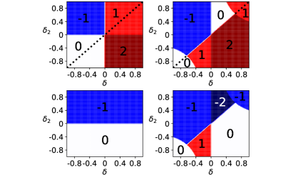
Figure 6: Phase diagrams for the topological invariants $I$ and $I_{3}$ for the $M=3$ leg ladder. A dotted line is placed where the analytical result from the main text, Eq. (6), applies. The top diagrams are for $I$ and the bottom diagrams are for $I_{3}$. Left panels: $z=0.0$, Right panels: $z=0.9$.

Appendix C Additional Chiral Symmetries and Topological Invariants

Here we give examples of additional chiral symmetries that can be defined under certain conditions. Take, for example, the case of the $M=2$ SSH ladder. Under the constraint $\delta_{1}=\delta_{2}$, we can define another chiral symmetry operator $\hat{S}_{2}$. The transformation is defined as

$$\hat{S}_{2}a_{j}^{1}\hat{S}_{2}^{-1}=-i{a_{j}^{2}}^{\dagger}\ ,\ \hat{S}_{2}a_{j}^{2}\hat{S}_{2}^{-1}=i{a_{j}^{1}}^{\dagger}$$

$$\hat{S}_{2}b_{j}^{1}\hat{S}_{2}^{-1}=i{b_{j}^{2}}^{\dagger}\ ,\ \hat{S}_{2}b_{j}^{2}\hat{S}_{2}^{-1}=-i{b_{j}^{1}}^{\dagger}$$ (C.1)

$$\hat{S}_{2}i\hat{S}_{2}^{-1}=-i.$$

One can compute the topological invariant $I_{2}$ corresponding to the chiral symmetry $\hat{S}_{2}$. One can switch $j\rightarrow k_{n}$ to get the corresponding symmetry in momentum space. Then we can use $\hat{S}\psi_{n}\hat{S}^{-1}=\sum_{m}(U_{S})_{n,m}^{*}\psi_{m}^{\dagger}$ to get the matrix $U_{S_{2}}(k)$. For this symmetry, we can work in the same basis as Eq. (A.2) for $M=2$. In this basis,

$$U_{S_{2}}(k)=\begin{pmatrix}0&0&0&i\\ 0&0&i&0\\ 0&-i&0&0\\ -i&0&0&0\end{pmatrix}.$$ (C.2)

Then we can plug this directly into Eq. (5) of the main text and solve numerically. We find that the invariant $I_{2}$ is zero for $-1<\delta_{1}=\delta_{2}<1$ and $-1<z<1$.

As another example, we consider the case of the $M=3$ SSH ladder. Suppose we have the constraint $\delta_{1}=\delta_{3}$. Then another chiral transformation is

$$\hat{S}_{3}a_{j}^{1}\hat{S}_{3}^{-1}={a_{j}^{3}}^{\dagger}\ ,\ \hat{S}_{3}a_{j}^{2}\hat{S}_{3}^{-1}=-{a_{j}^{2}}^{\dagger}\ ,\ \hat{S}_{3}a_{j}^{3}\hat{S}_{3}^{-1}={a_{j}^{1}}^{\dagger}$$

$$\hat{S}_{3}b_{j}^{1}\hat{S}_{3}^{-1}=-{b_{j}^{3}}^{\dagger}\ ,\ \hat{S}_{3}b_{j}^{2}\hat{S}_{3}^{-1}={b_{j}^{2}}^{\dagger}\ ,\ \hat{S}_{3}b_{j}^{3}\hat{S}_{3}^{-1}=-{b_{j}^{1}}^{\dagger}$$ (C.3)

$$\hat{S}_{3}i\hat{S}_{3}^{-1}=-i.$$

Similarly, in the same basis as Eq. (A.2) for $M=3$, we obtain

$$U_{S_{3}}(k)=\begin{pmatrix}0&0&1&0&0&0\\ 0&1&0&0&0&0\\ 1&0&0&0&0&0\\ 0&0&0&0&0&-1\\ 0&0&0&0&-1&0\\ 0&0&0&-1&0&0\end{pmatrix}.$$ (C.4)

Figure 6 shows a comparison of the invariants $I$ from the main text and $I_{3}$ defined here under the condition $\delta_{1}=\delta_{3}\equiv\delta$. A dotted line is placed where the analytical result from the main text, Eq. (6), applies. The magnitude of $I_{3}$ indicates the number of topological edge states protected by symmetry $\hat{S}_{3}$. Interestingly, for $z=0.9$ shown in the right panels of Fig. 6, there is a region where the invariant $I_{3}$ is equal to $-2$ while the invariant $I$ is equal to zero. In this region, there are two topological edge states protected by the symmetry $\hat{S}_{3}$.

Appendix D Density Matrix Elements

It is helpful to note

$$P^{A}A_{1}^{\dagger}A_{1}P^{A} = (A_{1}^{\dagger}A_{1}-A_{1}^{\dagger}A_{1}A_{2}^{\dagger}A_{2}),$$

$$P^{A}A_{1}^{\dagger}A_{2}P^{A} = A_{1}^{\dagger}A_{2}$$ (D.1)

and similarly for the $B$ operators. Now we simply list a few important equations. The matrix elements not listed are similar.

$$\langle P^{B}P^{A}P^{A}P^{B}\rangle=\langle P^{A}P^{B}\rangle=\langle A_{1}^{\dagger}A_{1}B_{1}^{\dagger}B_{1}\rangle$$

$$+\langle A_{1}^{\dagger}A_{1}B_{2}^{\dagger}B_{2}\rangle+\langle A_{2}^{\dagger}A_{2}B_{1}^{\dagger}B_{1}\rangle+\langle A_{2}^{\dagger}A_{2}B_{2}^{\dagger}B_{2}\rangle$$

$$-2\langle A_{1}^{\dagger}A_{1}B_{1}^{\dagger}B_{1}B_{2}^{\dagger}B_{2}\rangle-2\langle A_{2}^{\dagger}A_{2}B_{1}^{\dagger}B_{1}B_{2}^{\dagger}B_{2}\rangle$$

$$-2\langle A_{1}^{\dagger}A_{1}A_{2}^{\dagger}A_{2}B_{1}^{\dagger}B_{1}\rangle-2\langle A_{1}^{\dagger}A_{1}A_{2}^{\dagger}A_{2}B_{2}^{\dagger}B_{2}\rangle$$

$$+4\langle A_{1}^{\dagger}A_{1}A_{2}^{\dagger}A_{2}B_{1}^{\dagger}B_{1}B_{2}^{\dagger}B_{2}\rangle\qquad$$ (D.2)

$$\langle\Psi_{1,1}|A_{1}^{\dagger}B_{1}^{\dagger}B_{1}A_{1}|\Psi_{1,1}\rangle$$ (D.3)

$$=\frac{1}{\langle P^{A}P^{B}\rangle}(\langle A_{1}^{\dagger}A_{1}B_{1}^{\dagger}B_{1}\rangle-\langle A_{1}^{\dagger}A_{1}B_{1}^{\dagger}B_{1}B_{2}^{\dagger}B_{2}\rangle$$

$$-\langle A_{1}^{\dagger}A_{1}A_{2}^{\dagger}A_{2}B_{1}^{\dagger}B_{1}\rangle+\langle A_{1}^{\dagger}A_{1}A_{2}^{\dagger}A_{2}B_{1}^{\dagger}B_{1}B_{2}^{\dagger}B_{2}\rangle)$$

$$\langle\Psi_{1,1}|A_{1}^{\dagger}B_{1}^{\dagger}B_{2}A_{1}|\Psi_{1,1}\rangle$$ (D.4)

$$=\frac{1}{\langle P^{A}P^{B}\rangle}(\langle A_{1}^{\dagger}A_{1}B_{1}^{\dagger}B_{2}\rangle-\langle A_{1}^{\dagger}A_{1}A_{2}^{\dagger}A_{2}B_{1}^{\dagger}B_{2}\rangle)$$

$$\langle\Psi_{1,1}|A_{1}^{\dagger}B_{1}^{\dagger}B_{2}A_{2}|\Psi_{1,1}\rangle=\frac{1}{\langle P^{A}P^{B}\rangle}\langle A_{1}^{\dagger}A_{2}B_{1}^{\dagger}B_{2}\rangle$$ (D.5)

$$\langle\sigma_{z}^{a}\sigma_{z}^{b}\rangle_{1,1}=\frac{1}{\langle P^{A}P^{B}\rangle}(\langle A_{1}^{\dagger}A_{1}B_{1}^{\dagger}B_{1}\rangle-\langle A_{1}^{\dagger}A_{1}B_{2}^{\dagger}B_{2}\rangle$$

$$-\langle A_{2}^{\dagger}A_{2}B_{1}^{\dagger}B_{1}\rangle+\langle A_{2}^{\dagger}A_{2}B_{2}^{\dagger}B_{2}\rangle)\qquad$$ (D.6)

$$\langle\sigma_{z}^{a}\sigma_{x}^{b}\rangle_{1,1}=\frac{1}{\langle P^{A}P^{B}\rangle}(\langle A_{1}^{\dagger}A_{1}B_{1}^{\dagger}B_{2}\rangle+\langle A_{1}^{\dagger}A_{1}B_{2}^{\dagger}B_{1}\rangle$$

$$-\langle A_{2}^{\dagger}A_{2}B_{1}^{\dagger}B_{2}\rangle-\langle A_{2}^{\dagger}A_{2}B_{2}^{\dagger}B_{1}\rangle)\qquad$$ (D.7)

$$\langle\sigma_{x}^{a}\sigma_{z}^{b}\rangle_{1,1}=\frac{1}{\langle P^{A}P^{B}\rangle}(\langle B_{1}^{\dagger}B_{1}A_{1}^{\dagger}A_{2}\rangle+\langle B_{1}^{\dagger}B_{1}A_{2}^{\dagger}A_{1}\rangle$$

$$-\langle B_{2}^{\dagger}B_{2}A_{1}^{\dagger}A_{2}\rangle-\langle B_{2}^{\dagger}B_{2}A_{2}^{\dagger}A_{1}\rangle)\qquad$$ (D.8)

$$\langle\sigma_{x}^{a}\sigma_{x}^{b}\rangle_{1,1}=\frac{1}{\langle P^{A}P^{B}\rangle}(\langle A_{1}^{\dagger}A_{2}B_{1}^{\dagger}B_{2}\rangle+\langle A_{1}^{\dagger}A_{2}B_{2}^{\dagger}B_{1}\rangle$$

$$+\langle A_{2}^{\dagger}A_{1}B_{1}^{\dagger}B_{2}\rangle+\langle A_{2}^{\dagger}A_{1}B_{2}^{\dagger}B_{1}\rangle)\qquad$$ (D.9)

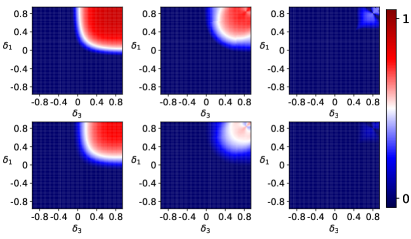
Figure 7: Comparison of the entanglement phase diagram based on $E_{\textrm{neg}}[\rho_{AB}^{1,1}]$ (top row) and $E_{F}[\rho_{AB}^{1,1}]$ (bottom row) in units of $\ln 2$ for a $3$-leg ladders with $L=16$ and $z=0.9$. Left to right: $\delta_{2}=-0.75$; $\delta_{2}=-0.25$; $\delta_{2}=0.25$.

Appendix E Entanglement of Formation

Here we consider the entanglement of formation as an alternative measure of bipartite entanglement of a mixed state. Given a density matrix $\rho$, we define the entanglement of formation as [42]

$$E_{F}(\rho)=\min\sum_{i}p_{i}E(|\psi_{i}\rangle)$$ (E.1)

where E is the pure state von-Neumann entanglement and the minimization is taken over all possible ensembles of the form $\rho=\sum_{i}p_{i}|\psi_{i}\rangle\langle\psi_{i}|$.

One of the problems with the entanglement of formation is the numerical difficulty of minimizing over all possible ensembles [43]. However, there is a method of obtaining the entanglement of formation for any two qubit system [44]. First, define a matrix $\tilde{\rho}=(\sigma_{y}\otimes\sigma_{y})\rho^{*}(\sigma_{y}\otimes\sigma_{y})$ where $\rho^{*}$ is the complex conjugate of the matrix $\rho$. Then define $R=\sqrt{\sqrt{\rho}\tilde{\rho}\sqrt{\rho}}$. and let $\lambda_{i}$ represent the eigenvalues of $R$ in decreasing order. The eigenvalues $\lambda_{i}$ are also the square roots of the eigenvalues of $\rho\tilde{\rho}$. The concurrence is then $C(\rho)=\max\{0,\lambda_{1}-\lambda_{2}-\lambda_{3}-\lambda_{4}\}$. Define a variable $x=\frac{1}{2}+\frac{1}{2}\sqrt{1-C^{2}(\rho)}$. The entanglement of formation is then $E_{F}=-x\ln(x)-(1-x)\ln(1-x)$. In Fig. 7, results for the $M=3$ SSH ladder are compared to the logarithmic negativity used in the main text. We can see that the results are virtually the same.

Appendix F Canonical/Grand Canonical Ensemble

In this work, we used Wick’s Theorem to calculate the n-point correlation functions. Wick’s Theorem, commonly used for non-interacting pure states, also has a version for ensemble calculations. Since the grand canonical ensemble has a factorizable density matrix, Wick’s Theorem for the grand canonical case is similar to the pure state case [45]. Consider an operator

$$A_{k_{1},k_{2},\dots,k_{m},\ell_{1},\ell_{2},\dots,\ell_{m}}=c^{\dagger}_{k_{1}}c^{\dagger}_{k_{2}}\dots c^{\dagger}_{k_{m}}c_{\ell_{m}}\dots c_{\ell_{2}}c_{\ell_{1}}$$ (F.1)

where none of the indices $k_{i}$ are the same, none of the indices $l_{i}$ are the same and the $c$ operators are in an arbitrary basis. Define an $m\times m$ matrix $(\langle c^{\dagger}c\rangle)_{i,j}=\langle c^{\dagger}_{k_{i}}c_{l_{j}}\rangle$. Then for pure states and in the grand canonical ensemble

$$\langle A_{k_{1},k_{2},\dots,k_{m},\ell_{1},\ell_{2},\dots,\ell_{m}}\rangle=\text{det}\langle c^{\dagger}c\rangle.$$ (F.2)

For the grand canonical ensemble, we can use the Fermi-Dirac distribution for the occupation number $n_{i}=c^{\dagger}_{i}c_{i}$ expectation value in the diagonal basis [46]

$$\langle n_{i}\rangle=\frac{1}{1+e^{\beta(\epsilon_{i}-\mu)}}.$$ (F.3)

In the grand canonical ensemble, we set the chemical potential $\mu=0$ in order to preserve particle-hole symmetry. For the canonical ensemble, (F.2) and (F.3) are not satisfied. In the canonical ensemble, multi-point correlators can be written in terms of two point correlators in the diagonal basis as

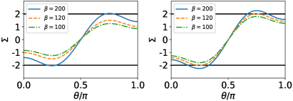
Figure 8: $\Sigma$, as defined in Eq. (9) of the main text, for a 3-leg ladder with $L=8$, $\delta_{1}=0.29$, $\delta_{2}=-0.99$, $\delta_{3}=0.99$ and $z=0.95$ for various inverse temperatures $\beta=1/T$. Left panel: Grand canonical ensemble with chemical potential $\mu=0$. Right panel: Canonical ensemble.

$$\langle n_{\ell_{1}}n_{\ell_{2}}\dots n_{\ell_{m}}\rangle=\sum_{i=1}^{m}\langle n_{\ell_{i}}\rangle\prod_{j(\neq i)}^{m}\frac{e^{\beta\epsilon_{\ell_{i}}}}{e^{\beta\epsilon_{\ell_{i}}}-e^{\beta\epsilon_{\ell_{j}}}}.$$ (F.4)

Note that the equation above is only valid if all of the energy levels $\epsilon_{\ell_{i}}$ are nondegenerate, which we have verified numerically for the results in this section. The distribution $\langle n_{i}\rangle$ itself has to be calculated using a numerically stable recursion relation [47]. Figure 8 shows the breaking of the Bell’s inequality for $\Sigma$ as defined in Eq. (9) of the main text. The grand canonical ensemble breaks the inequality for $\beta$ as low as $200$ and the canonical ensemble breaks the inequality for $\beta$ as low as $120$. For a cold atomic gas experiment—neglecting particle loss—the question whether the canonical or the grand-canonical ensemble are more appropriate depends on how well-controlled the particle number for each realization is. As expected, stronger quantum correlations are preserved to higher temperatures in the canonical ensemble.

References

- Wiseman and Vaccaro [2003] H. M. Wiseman and J. A. Vaccaro, Phys. Rev. Lett. 91, 097902 (2003), URL https://link.aps.org/doi/10.1103/PhysRevLett.91.097902.
- Dowling et al. [2006] M. R. Dowling, A. C. Doherty, and H. M. Wiseman, Phys. Rev. A 73, 052323 (2006), URL https://link.aps.org/doi/10.1103/PhysRevA.73.052323.
- Schuch et al. [2004a] N. Schuch, F. Verstraete, and J. I. Cirac, Phys. Rev. Lett. 92, 087904 (2004a), URL https://link.aps.org/doi/10.1103/PhysRevLett.92.087904.
- Schuch et al. [2004b] N. Schuch, F. Verstraete, and J. I. Cirac, Phys. Rev. A 70, 042310 (2004b), URL https://link.aps.org/doi/10.1103/PhysRevA.70.042310.
- Klich and Levitov [2008] I. Klich and L. S. Levitov, arXiv:0812.0006 (2008).
- Rakovszky et al. [2019] T. Rakovszky, C. W. von Keyserlingk, and F. Pollmann, Phys. Rev. B 100, 125139 (2019), URL https://link.aps.org/doi/10.1103/PhysRevB.100.125139.
- Bonsignori et al. [2019] R. Bonsignori, P. Ruggiero, and P. Calabrese, Journal of Physics A: Mathematical and Theoretical 52, 475302 (2019), URL https://doi.org/10.1088%2F1751-8121%2Fab4b77.
- Murciano et al. [2020a] S. Murciano, G. D. Giulio, and P. Calabrese, SciPost Phys. 8, 46 (2020a), URL https://scipost.org/10.21468/SciPostPhys.8.3.046.
- Murciano et al. [2020b] S. Murciano, G. D. Giulio, and P. Calabrese, JHEP 2020, 73 (2020b).
- Barghathi et al. [2019] H. Barghathi, E. Casiano-Diaz, and A. Del Maestro, Phys. Rev. A 100, 022324 (2019), URL https://link.aps.org/doi/10.1103/PhysRevA.100.022324.
- Lukin et al. [2019] A. Lukin, M. Rispoli, R. Schittko, M. E. Tai, A. M. Kaufman, S. Choi, V. Khemani, J. Léonard, and M. Greiner, Science 364, 256 (2019), URL https://science.sciencemag.org/content/364/6437/256.full.pdf.
- Kiefer-Emmanouilidis et al. [2020a] M. Kiefer-Emmanouilidis, R. Unanyan, J. Sirker, and M. Fleischhauer, SciPost Phys. 8, 083 (2020a).
- Kiefer-Emmanouilidis et al. [2020b] M. Kiefer-Emmanouilidis, R. Unanyan, M. Fleischhauer, and J. Sirker, Phys. Rev. Lett. 124, 243601 (2020b).
- Ryu et al. [2010] S. Ryu, A. P. Schnyder, A. Furusaki, and A. W. W. Ludwig, New Journal of Physics 12, 065010 (2010).
- Chiu et al. [2016] C.-K. Chiu, J. C. Y. Teo, A. P. Schnyder, and S. Ryu, Rev. Mod. Phys. 88, 035005 (2016), URL https://link.aps.org/doi/10.1103/RevModPhys.88.035005.
- Bakr et al. [2009] W. S. Bakr, J. I. Gillen, A. Peng, S. Fölling, and M. Greiner, Nature 462, 74 (2009), eprint 0908.0174.
- Sherson et al. [2010] J. F. Sherson, C. Weitenberg, M. Endres, M. Cheneau, I. Bloch, and S. Kuhr, Nature 467, 68 (2010).
- Bell [1964] J. S. Bell, Physics Physique Fizika 1, 195 (1964), URL https://link.aps.org/doi/10.1103/PhysicsPhysiqueFizika.1.195.
- Bell [1966] J. S. Bell, Rev. Mod. Phys. 38, 447 (1966), URL https://link.aps.org/doi/10.1103/RevModPhys.38.447.
- Clauser et al. [1969] J. F. Clauser, M. A. Horne, A. Shimony, and R. A. Holt, Phys. Rev. Lett. 23, 880 (1969), URL https://link.aps.org/doi/10.1103/PhysRevLett.23.880.
- Haroche [2006] S. Haroche, J.-M. Raimond, Exploring the Quantum: Atoms, Cavities and Photons (Oxford University Press, New York, 2006).
- Aspect et al. [1982] A. Aspect, P. Grangier, and G. Roger, Phys. Rev. Lett. 49, 91 (1982), URL https://link.aps.org/doi/10.1103/PhysRevLett.49.91.
- Su et al. [1979] W. Su, J. Schrieffer, and A. Heeger, Phys. Rev. Lett. 42, 1698 (1979).
- Heeger et al. [1988] A. J. Heeger, S. Kivelson, J. R. Schrieffer, and W. P. Su, Rev. Mod. Phys. 60, 781 (1988).
- Atala et al. [2013] M. Atala, M. Aidelsburger, J. T. Barreiro, D. Abanin, T. Kitagawa, E. Demler, and I. Bloch, Nat. Phys. 9, 795 (2013).
- Xie et al. [2019] D. Xie, W. Gou, T. Xiao, B. Gadway, and B. Yan, NPJ Quantum Information 5, 55 (2019).
- Meier et al. [2016] E. J. Meier, F. A. An, and B. Gadway, Nat. Comm. 7, 13986 (2016).
- Meyrath et al. [2005] T. P. Meyrath, F. Schreck, J. L. Hanssen, C.-S. Chuu, and M. G. Raizen, Phys. Rev. A 71, 041604 (2005), URL https://link.aps.org/doi/10.1103/PhysRevA.71.041604.
- Gaunt et al. [2013] A. L. Gaunt, T. F. Schmidutz, I. Gotlibovych, R. P. Smith, and Z. Hadzibabic, Phys. Rev. Lett. 110, 200406 (2013), URL https://link.aps.org/doi/10.1103/PhysRevLett.110.200406.
- Wakatsuki et al. [2014a] R. Wakatsuki, M. Ezawa, Y. Tanaka, and N. Nagaosa, Phys. Rev. B 90, 014505 (2014a), URL https://link.aps.org/doi/10.1103/PhysRevB.90.014505.
- Gurarie [2011] V. Gurarie, Phys. Rev. B 83, 085426 (2011), URL https://link.aps.org/doi/10.1103/PhysRevB.83.085426.
- Padavić et al. [2018] K. Padavić, S. S. Hegde, W. DeGottardi, and S. Vishveshwara, Phys. Rev. B 98, 024205 (2018), URL https://link.aps.org/doi/10.1103/PhysRevB.98.024205.
- Dagotto and Rice [1996] E. Dagotto and T. M. Rice, Science 271, 618 (1996), ISSN 0036-8075, URL https://science.sciencemag.org/content/271/5249/618.
- Horodecki et al. [2009] R. Horodecki, P. Horodecki, M. Horodecki, and K. Horodecki, Rev. Mod. Phys. 81, 865 (2009), URL https://link.aps.org/doi/10.1103/RevModPhys.81.865.
- Życzkowski et al. [1998] K. Życzkowski, P. Horodecki, A. Sanpera, and M. Lewenstein, Phys. Rev. A 58, 883 (1998), URL https://link.aps.org/doi/10.1103/PhysRevA.58.883.
- Vidal and Werner [2002] G. Vidal and R. F. Werner, Phys. Rev. A 65, 032314 (2002), URL https://link.aps.org/doi/10.1103/PhysRevA.65.032314.
- Fölling et al. [2005] S. Fölling, F. Gerbier, A. Widera, O. Mandel, T. Gericke, and I. Bloch, Nature 434, 481 (2005).
- Bures [1969] D. Bures, Trans. Am. Math. Soc. 135, 199 (1969).
- Uhlmann [1976] A. Uhlmann, Rep. Math. Phys. 9, 273 (1976).
- Zanardi et al. [2007] P. Zanardi, H. T. Quan, X. Wang, and C. P. Sun, Phys. Rev. A 75, 032109 (2007).
- Campos Venuti et al. [2011] L. Campos Venuti, N. T. Jacobson, S. Santra, and P. Zanardi, Phys. Rev. Lett. 107, 010403 (2011), URL https://link.aps.org/doi/10.1103/PhysRevLett.107.010403.
- Bennett et al. [1996] C. H. Bennett, D. P. DiVincenzo, J. A. Smolin, and W. K. Wootters, Phys. Rev. A 54, 3824 (1996), URL https://link.aps.org/doi/10.1103/PhysRevA.54.3824.
- Huang [2014] Y. Huang, New Journal of Physics 16, 033027 (2014).
- Wootters [1998] W. K. Wootters, Phys. Rev. Lett. 80, 2245 (1998), URL https://link.aps.org/doi/10.1103/PhysRevLett.80.2245.
- Schonhammer [2017] K. Schönhammer, Phys. Rev. A 96, 012102 (2017), URL https://link.aps.org/doi/10.1103/PhysRevA.96.012102.
- Shapourian and Ryu [2019] H. Shapourian and S. Ryu, Journal of Statistical Mechanics: Theory and Experiment 2019, 043106 (2019), URL https://doi.org/10.1088.
- Borrmann [1999] P. Borrmann, J. Harting, O. Mülken, and E. R. Eberhard, Phys. Rev. A 60, 1519 (1999), URL https://link.aps.org/doi/10.1103/PhysRevA.60.1519.