A Simple Electrostatic Model for the Hard-Sphere Solute Component of Nonpolar Solvation

Abstract

We propose a new model for estimating the free energy of forming a molecular cavity in a solvent, by assuming this energy is dominated by the electrostatic energy associated with creating the static (interface) potential inside the cavity. The new model approximates the cavity-formation energy as that of a shell capacitor: the inner, solute-shaped conductor is held at the static potential, and the outer conductor (at the first solvation shell) is held at zero potential. Compared to cavity energies computed using free-energy pertubation with explicit-solvent molecular dynamics, the new model exhibits surprising accuracy (Mobley test set, RMSE 0.45 kcal/mol). Combined with a modified continuum model for solute-solvent van der Waals interactions, the total nonpolar model has RMSE of 0.55 kcal/mol on this test set, which is remarkable because the two terms largely cancel. The overall nonpolar model has a small number of physically meaningful parameters and compares favorably to other published models of nonpolar solvation. Finally, when the proposed nonpolar model is combined with our solvation-layer interface condition (SLIC) continuum electrostatic model, which includes asymmetric solvation-shell response, we predict solvation free energies with an RMS error of 1.35 kcal/mol relative to experiment, comparable to the RMS error of explicit-solvent FEP (1.26 kcal/mol). Moreover, all parameters in our model have a clear physical meaning, and employing reasonable temperature dependencies yields remarkable correlation with solvation entropies.

I Introduction

Interactions between a solute molecule and a surrounding solvent are of fundamental importance across chemistry, biology, and associated fields of science and engineering. Fully atomistic, explicit-solvent molecular dynamics (MD) simulations provide an accurate and chemically detailed understanding of these interactions, but can be prohibitively resource intensive. Implicit-solvent models Roux and Simonson (1999) require orders of magnitude less computation, but historically their accuracy has been lower than those of explicit-solvent calculations, limiting the scope of possible applications Bardhan (2012). Implicit-solvent models have a rigorous statistical-mechanical basis Roux and Simonson (1999), and can be understood and assessed through the notion of the solvation free energy $\Delta G_{solv}$, the free energy associated with transferring a given solute from gas phase to solvent. The solvation free energy is frequently decomposed as a sum of two components, the nonpolar ($\Delta G_{np}$) and polar ($\Delta G_{es}$) terms. The polar term is the free energy of creating the solute’s charge distribution inside a pre-existing solute cavity, and frequently modeled with macroscopic continuum dielectric theory, e.g. the Poisson-Boltzmann equation.

The present paper focuses on the nonpolar component: the work required to place an uncharged solute inside the solvent. Implicit-solvent models often treat $\Delta G_{np}$ as a weighted combination of the solute’s solvent-accessible surface area (SASA) and other geometric measures Gallicchio et al. (2002); Swanson et al. (2004); Wong et al. (2009); Wang et al. (2019), e.g. $\Delta G_{np}=\gamma(SASA)+b$, where $\gamma$ is usually interpreted as the liquid-vapor surface tension, and $b$ is a scaling constant (sometimes presented as $pV$, pressure times volume). Nevertheless, the well-known inaccuracies of SASA-based models Gallicchio et al. (2000); Wagoner and Baker (2004); Mobley et al. (2009); Mehdizadeh Rahimi et al. (2019) motivate significant research to improve them Dzubiella et al. (2006); Cheng et al. (2009); Nguyen and Wei (2017); Wang et al. (2018). The nonpolar term can itself be decomposed into a sum of two free energies Zacharias (2003): $\Delta G_{cav}$, the creation of a solute-shaped cavity by turning on the short-range repulsive interactions (also known as the creation of the hard-sphere solute), and $\Delta G_{disp}$, in which one turns on the longer-range attractive dispersion interactions. In an explicit-solvent description, this is similar to the Weeks-Chandler-Andersen (WCA) theory Weeks et al. (1971), where one performs MD simulations using a Lennard-Jones potential decomposed into short- and long-range components. Using MD with umbrella sampling, $\Delta G_{cav}$ can also be computed using Lum-Chandler-Weeks (LCW) theory Lum et al. (1999); Huang et al. (2001); Varilly et al. (2011).

The present study on nonpolar solvation is an outgrowth of our longstanding interest in modeling Poisson–Boltzmann (PB) electrostatics using boundary-integral equations Cooper et al. (2014); Altman et al. (2006, 2009); Bardhan and Knepley (2014); Molavi Tabrizi et al. (2017). Recognizing that our proposed model is rather unusual, we review this work briefly, to introduce key ideas and motivate our approach. While using explicit-solvent free-energy pertubation (FEP) MD to parameterize a multiscale PB model Bardhan (2011, 2013), we learned that charge-sign asymmetry errors dominated the differences between standard and multiscale PB Bardhan et al. (2012), and we identified two distinct sources of charge-sign asymmetry. First, water hydrogens can approach solute charges closer than the larger water oxygens. The second, central to the present work, is the presence of a significant electrostatic potential in a completely uncharged solute, which is created by the solvent structure immediately surrounding the solute  Ashbaugh (2000); Cerutti et al. (2007); Beck (2013) (see, in particular, Fig. 1 of Cerutti et al. (2007)). We called this the static potential Ashbaugh (2000), because it remains when the solute charge distribution is zero everywhere (the familiar reaction potential Roux and Simonson (1999) vanishes in the absence of solvent charges). Noting that the static potential is nearly constant ($\sim\!10$ kcal/mol/$e$) within even complex molecules Cerutti et al. (2007), we approximated it as constant and developed a modified dielectric model to account for the steric asymmetry. We called this the SLIC (solvation-layer interface condition) electrostatic model Bardhan and Knepley (2014); Molavi Tabrizi et al. (2017), and found it sufficiently improved over standard PB that we began to test its performance on total solvation free energies, using the traditional SASA model Gallicchio et al. (2002) for $\Delta G_{np}$. Our recent study Mehdizadeh Rahimi et al. (2019) showed SLIC/SASA approaching MD in overall accuracy on the Mobley test set Mobley et al. (2009), despite the fact that the SASA model exhibits a weak overall correlation with explicit-solvent MD results for $\Delta G_{np}$. The disparity motivated exploring possible improvements to nonpolar solvation models (others have highlighted this recently as well Knight and Brooks III (2011)).

The static potential’s existence—and its importance in solvation electrostatics—lead to an apparent paradox: namely, it implies that the solute’s nonpolar solvation free energy includes an electrostatic term, which represents the work done creating the static potential inside the solute. Consider that the static potential field exists in an uncharged solute, i.e., after one creates the solute atoms (as uncharged Lennard-Jones particles, for many FEP calculations). However, far from the solute, the potential is zero—again, constant. The potential varies significantly only in the solvation shell, indicating a non-zero electric field (and therefore energy density) there. Therefore, the thermodynamic steps associated with nonpolar solvation include an electrostatic work. The present paper asks, “How important is this electrostatic work in nonpolar solvation free energies?” and models the electrostatic problem very simply, as a capacitor in which the molecular solute is treated as a body held at constant potential (the static potential) and the bulk solvent volume treated as a ground (zero potential). We find that this capacitor model reproduces explicit-solvent cavity free energies with surprisingly high accuracy, enabling an overall implicit-solvent model that is comparable in accuracy to explicit-solvent calculations.

II Theory and Methods

We model the nonpolar solvation free energy $\Delta G_{np}=\Delta G_{cav}+\Delta G_{disp}$, so the solvation free energy is $\Delta G_{solv}=\Delta G_{cav}+\Delta G_{disp}+\Delta G_{es}$. We propose a capacitance-based model for $\Delta G_{cav}$, and combine it with a modification of a continuum integral method for calculating $\Delta G_{disp}$ Floris and Tomasi (1989); Levy et al. (2003); Sulea et al. (2009), using SLIC continuum electrostatics Bardhan and Knepley (2014); Molavi Tabrizi et al. (2017); Mehdizadeh Rahimi et al. (2019) without modification to compute $\Delta G_{es}$.

We model the potential inside the solute as the constant $\phi_{{static}}$, defining the solute boundary as the solvent-excluded surface (SES) Connolly (1983). In the infinite solvent region, we model the potential as $\phi=0$, and bound the region using the boundary of the first solvation shell (the solvent-accessible surface, SAS Connolly (1983)). These surfaces bound a shell, which we model as a macroscopic dielectric with the uniform relative permittivity $\epsilon_{shell}$, and where the electrostatic potential obeys the Laplace equation (see SI Figure 1 and derivation in Supporting Information). The fixed potentials at the boundaries mean that the dielectric constants of the solute and bulk solvent are irrelevant. We use $\epsilon_{shell}$ as a fitting parameter, but it has clear physical bounds and significance. The energy associated with this boundary-value problem can be solved using a pair of coupled boundary-integral equations for unknown charge densities on the two surfaces,

$$\left[\begin{array}[]{c c}V_{diel}&V_{diel}\\ V_{shell}&V_{shell}\end{array}\right]\left[\begin{array}[]{c}\sigma_{diel}\\ \sigma_{shell}\end{array}\right]=\epsilon_{shell}\left[\begin{array}[]{c}\phi_{static}\\ 0\end{array}\right],$$ (1)

where $V_{diel}(\psi_{shell})=\oint_{shell}\frac{\psi(\mathbf{r}^{\prime})}{4\pi|\mathbf{r}_{diel}-\mathbf{r}^{\prime}|}\text{d}\mathbf{r}^{\prime}$ denotes the potential induced at the inner surface (the dielectric boundary) by the surface charge distribution on the outer boundary (the solvent-accessible surface). Having found the surface charge distributions, and noting that the potential on the outer surface is zero, we can compute the energy with

$$\Delta G_{cav}=\oint_{diel}\phi_{static}\sigma_{diel}(\mathbf{r})\text{d}\mathbf{r}.$$ (2)

Our model therefore treats $\Delta G_{cav}$ as the free energy required to create the interface potential inside the solute. This continuum description can also be seen as the free energy of the solvent-solvent electrostatic interactions as molecules accommodate around the cavity, which is related to the so-called reorganization energy Lee (1985); Yu and Karplus (1988); Lazaridis (1998, 2000); Gallicchio et al. (2000) (Supporting Information). The surface charge layers approximate the behavior of first-shell solvent molecules: when water surrounds a completely uncharged cavity, hydrogens generally point inward, while oxygens are further out Cerutti et al. (2007). This creates a kind of diffuse double layer of charge, so $\sigma_{diel}$ roughly captures the water hydrogen charge distribution and $\sigma_{shell}$ represents the water oxygens at the SAS.

We parameterized the molecules with GAFF Wang et al. (2004) and discretized the SES and SAS into flat triangular panels (boundary elements) with the msms package Sanner et al. (1995), using a $1.4$ Å-radius probe sphere and taking every atom’s radius to be $r_{min}/2$ without adjustment. We then solved for $\sigma_{diel}$ and $\sigma_{shell}$ with a boundary-element method (BEM) using the bempp library. Śmigaj et al. (2015) Specifically, we use bempp’s implementation of BEM to generate a finite-dimensional approximation to Equation (1) by approximating $\sigma_{diel}$ and $\sigma_{shell}$ as piecewise constant on each boundary element, and employing a Galerkin discretization to generate a matrix equation, which we solve using GMRES Saad and Schultz (1986). We set $\phi_{static}=10.7$ kcal/mol/$e$, following previous work Bardhan and Knepley (2014), and $\epsilon_{shell}=7.75$ (obtained by an empirical single-parameter fitting).

We calculate $\Delta G_{disp}$ by integrating the Lennard-Jones potential outside the solvent-accessible surface Floris and Tomasi (1989); Levy et al. (2003); Sulea et al. (2009), using the divergence theorem to reformulate it as a surface integral

$$\Delta G_{disp}=\sum_{i}\oint_{shell}\rho_{w}\frac{\partial}{\partial\mathbf{n}}\left(\frac{A_{i}}{90|\mathbf{r}-\mathbf{r}_{i}|^{10}}-\frac{B_{i}}{12|\mathbf{r}-\mathbf{r}_{i}|^{4}}\right)\text{d}\mathbf{r}$$ (3)

where $\rho_{w}$ is the solvent number density (0.0366 Å^-3 for water), $A_{i}$ and $B_{i}$ are related to the Lennard-Jones parameters for the water oxygen and atom $i$, the sum is over the solute’s atoms, and the unit vector $\mathbf{n}$ points into the solvent Bardhan et al. (2007). We found that this model correlates highly with explicit-solvent free energy calculations for $\Delta G_{disp}$, but exhibits a systematic underprediction that correlates highly with surface area. This continuum Lennard-Jones model treats water density as uniform even though it is known to increase near interfaces Beglov and Roux (1996, 1997); Lake and McCullagh (2017), so we tested a simple correction in which we allowed water number density in the first solvation shell (outside the SAS) to be higher than bulk; we have used $1.8\rho_{w}$ here (see Supporting Information) Lake and McCullagh (2017).

In our model for $\Delta G_{np}$, all fitting parameters have clear physical significance, and their optimized values can be at least compared to quantities that are determined relatively easily from experiment or simulation. For instance, $\epsilon_{shell}$ is between $1$ and $80$ but much closer to 1, with evidence that the permittivity near interfaces depends on the local radius of curvature Dinpajooh and Matyushov (2016). One can also compute $\phi_{static}$ from explicit-solvent simulations Cerutti et al. (2007); Bardhan et al. (2012); for spherical solutes, it varies only slightly with radius Ashbaugh (2000). In this work, the SLIC parameters were $\alpha=0.898$, $\beta=-30.476$, $\gamma=-0.151$, $\mu=-0.449$, and $\phi=0.095$; these were obtained by optimizing SLIC to reproduce explicit-solvent FEP charging free energies Molavi Tabrizi et al. (2017); Mehdizadeh Rahimi et al. (2019).

III Results and Discussion

We computed the nonpolar solvation energy of $498$ small solutes from the well-known Mobley test set and compared our results to Mobley’s explicit-solvent free-energy perturbation (FEP) calculations Mobley et al. (2009). Figures 1, 2, and 3 are plots of our proposed models for $\Delta G_{cav}$, $\Delta G_{disp}$, and $\Delta G_{np}$, respectively, compared to Mobley’s calculations of the same quantities Mobley . In each figure, the segmented lines correspond to perfect accuracy; the dotted lines in Figure 3 correspond to $\pm\;1$-kcal/mol offsets. We measured accuracy using the Pearson coefficient ($\rho_{p}$), the root mean square of the difference (RMSD), and the mean unsigned error (MUE); these are given in the figure captions. The figures show excellent correlation, with $\rho_{p}=0.88$, RMSD=0.55 kcal/mol, and MUE=0.38 kcal/mol for $\Delta G_{np}$, somewhat lower than for $\Delta G_{cav}$ and $\Delta G_{disp}$, but notable because it is still high despite the fact that $\Delta G_{np}$ is the sum of two large quantities with opposing signs, posing a challenge to model accurately unless the errors are highly correlated.

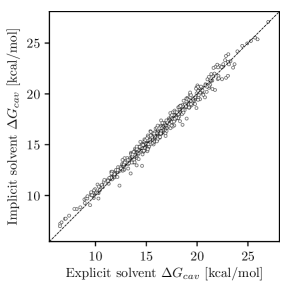
Figure 1: The proposed implicit-solvent model for $\Delta G_{cav}$, compared to explicit-solvent FEP Mobley et al. (2009) ($\rho_{p}=0.99$, RMSD=$0.45$ kcal/mol, MUE=$0.36$ kcal/mol).

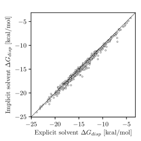
Figure 2: The proposed implicit-solvent model for $\Delta G_{disp}$, compared to explicit-solvent FEP ($\rho_{p}=0.99$, RMSD=$0.50$ kcal/mol, MUE=$0.38$ kcal/mol).

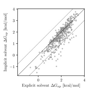
Figure 3: The proposed implicit-solvent model for $\Delta G_{np}$, compared to explicit-solvent FEP ($\rho_{p}=0.88$, RMSD=$0.55$ kcal/mol, MUE=$0.38$ kcal/mol).

The proposed model for $\Delta G_{cav}$ explicitly only includes electrostatics, although clearly electrostatics are not the only contribution (Supporting Information). The fact that the model’s predictions agree with explicit-solvent calculations indicates that either the electrostatics dominate over other terms in the cavity free energy, or that the dominant components have similar functional forms (e.g. the excellent correlation with SASA Mobley et al. (2009)). It is also interesting to note that even though the solvent reorganization energy is usually considered to cancel out in hard-sphere solute solvation Lee (1985); Yu and Karplus (1988); Gallicchio et al. (2000), our model for the associated mean-field electrostatics provides an excellent predictor of cavity free energies. This result is supported by previous observations on the importance of the reorganization energy in solvation free energy Lazaridis (1998, 2000), and reconsiders the role of electrostatics in nonpolar solvation.

Combining SLIC electrostatic calculations on this test set Bardhan and Knepley (2014) (SI Figure 4) with our nonpolar model then yields the total $\Delta G_{solv}$. Figure 4 is a plot of the full implicit-solvent model’s correlation with explicit-solvent FEP solvation free energies (SI Figure 5 is a plot of the correlation with experiment). Our implicit-solvent model performs well compared to both explicit-solvent MD results ($\rho_{p}=0.97$, RMSD=$1.02$ kcal/mol, and MUE=$0.72$ kcal/mol) and experiment ($\rho_{p}=0.92$, RMSD=$1.35$ kcal/mol, and MUE=$1.01$ kcal/mol).

These measures are remarkably comparable to those from explicit-solvent FEP ($\rho_{p}=0.94$, RMSD=$1.26$ kcal/mol, and MUE=$1.04$ kcal/mol). Beyond these correspondences, the distribution of errors for the implicit-solvent and explicit-solvent models are very similar (Figure 5), suggesting that physics-based implicit-solvent models may be approaching parity with explicit-solvent MD.

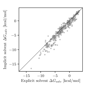
Figure 4: Correlation of $\Delta G_{solv}$ with MD ($\rho_{p}=0.97$, RMSD=$1.03$ kcal/mol, MUE=$0.72$ kcal/mol).

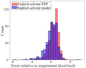
Figure 5: Histograms of errors relative to experiment, for explicit-solvent FEP calculations by Mobley et al., and for the proposed implicit-solvent model ($\rho_{p}=0.92$, RMSD=$1.35$ kcal/mol, MUE=$1.01$ kcal/mol)

.

Table 1: Comparison with DISA model Michael et al. (2017). RMSD and MUE are in kcal/mol.

Model	$\rho_{p}$	RMSD	MUE
DISA	0.82	0.34	0.25
Present work	0.92	0.27	0.20

We also compared our proposed nonpolar model to other existing implicit-solvent approaches. A recent study Michael et al. (2017) assessed the performance of different SASA models, using 35 alkanes and 27 polar molecules from the Mobley test set. The authors obtained the best results using the DISA (dispersion integral surface area) model, which combines a SASA scheme for $\Delta G_{cav}$ and an integral method Aguilar et al. (2010) for $\Delta G_{disp}$. Table 1 shows how the DISA model and our approach compare with MD for these solutes. Further, the authors found that the most accurate results were obtained when one used a molecule-dependent surface tension—which ranged from $\gamma=-50$ to $\gamma=20$ kcal/mol/Å, depending on whether the solute was polar, aromatic, an alkane, or an ion Michael et al. (2017). Similar dependencies on solute type have been observed previously Ashbaugh et al. (1999). The dependence of the optimal surface tension on solute type highlights the incomplete physical picture from SASA models: from the statistical-mechanical perspective Roux and Simonson (1999), the nonpolar solvation free energy assumes a completely uncharged molecule (a set of Lennard-Jones particles), and therefore a physically consistent model should not depend significantly on atomic charges. Our model also presents a stronger physical basis for calculating $\Delta G_{disp}$; the dispersion integral part of DISA relies on two fitting parameters that to our understanding lack physical interpretation Aguilar et al. (2010). In our model for $\Delta G_{disp}$, the only fitting parameters are the shell width and the number density of water molecules near the interface, which is a physical quantity known to be higher than bulk (set here to $1.8\rho_{w}$). Similarly, our capacitor approximation for $\Delta G_{cav}$ uses the same parameters ($\epsilon_{shell}$ and $\phi_{static}$) for all the solutes in Mobley’s test set, which includes alkane, polar, and aromatic molecules. Despite the smaller number of free parameters, which are all independent of the solute, our parameterized model outperforms DISA (Table 1).

The Supporting Information provides additional results, including for spherical solutes, correlations with SASA, and a proof-of-concept calculation of entropy. In particular, SI Figure 3 shows that SASA correlates linearly with both $\Delta G_{cav}$ and $\Delta G_{disp}$, but exhibits poorer correlation with $\Delta G_{np}$ (SI Figure 5), as observed previously for explicit MD calculations Mobley et al. (2009). Furthermore, SI Figure 10 shows the notable correlation of $T\Delta S$ computed with our model, compared with experiments, using physically reasonable variations of $\phi_{static}$ and $\rho_{w}$ with temperature.

IV Summary and Future Work

The main contribution of this paper is a new approach for estimating the free energy of forming the solute cavity. Recognizing that the mean electrostatic potential in the (uncharged) cavity is large and approximately constant, and that the mean electrostatic potential outside the solvation layer is zero, we proposed modeling $\Delta G_{cav}$ as a macroscopic capacitor—essentially, the solute-shaped version of a spherical capacitor with two concentric, conducting shells. From a purely atomistic point of view, the charge structure and electric field in the hydration shell are highly complex. However, because we were interested in the magnitude of the work required to create the static potential in the uncharged solute, we proposed a very simple model to estimate the total energy stored in the field—neglecting the atomistic details of the charge structure and instead assuming a relatively smooth field. We found to our surprise that this work corresponded closely to the total cavity free energy. Our proposed model suggests a previously underappreciated role for electrostatics in solvation: namely, an electrostatic contribution to the Gibbs free energy of cavity formation.

We have modeled $\Delta G_{disp}$ with a modified integral-type continuum model, in which one sums over all solute atoms the volume integral of the atom’s Lennard-Jones interactions with the solvent. We found that our implementation of the standard integral approach systematically underpredicted $\Delta G_{disp}$. We improved the predictions significantly by allowing higher-than-bulk solvent density in the hydration shell, in accordance with experimental and simulation results; previous such models assumed the solvent density to be bulk everywhere. Given the accuracy of WCA nonpolar energies Wagoner and Baker (2006), efforts to improve WCA models may benefit from similarly granular comparisons.

We have validated the overall model (capacitance-based cavity free energy, modified continuum integral dispersion, and SLIC electrostatics) against explicit-solvent MD free-energy calculations and found that it predicts nonpolar solvation free energies more accurately than models based on the common solvent-accessible surface-area (SASA) model. Importantly, our model achieves this accuracy without employing individual atomic radii as fitting parameters in any of the three energy terms. The nonpolar and the electrostatic terms use the same underlying atomic radii from the MD force field ($r_{min}/2$), with a uniform scaling for SLIC electrostatics such that for any atom $r_{implicit}=0.92r_{min}/2$. This uniform scaling factor of 0.92 was set in our first study of the SLIC continuum electrostatic model Bardhan and Knepley (2014), and we have not attempted to reparameterize or find a different scaling factor since the original paper. The parameters of our proposed model (static potential, permittivity, and solvation-shell number density) have robust physical interpretations that are largely intrinsic to the solvent, and do not depend on solute type or atom types. We highlight this aspect of our model because the thermodynamic cycles often drawn to distinguish contributions to the nonpolar solvation free energy involve processes in which the associated models should not depend strongly on atom type or solute size. We acknowledge that our model’s parameters do have a minor dependence, see e.g. Ashbaugh (2000) for the variation in static potential with solute size, but even as a fitting parameter, it is one that works for all solute types tested so far. Also, although the precise values used in the proposed model may be viewed to some extent as fitted parameters, the model gives accurate results for physically reasonable values. The correlation of such a simple model with explicit-solvent MD seems notable, especially considering the small number of fitting parameters.

We have also found that our capacitance-based model for $\Delta G_{cav}$ exhibits a temperature dependence that correlates surprisingly well with solvation entropies when one uses a reasonable value for the temperature dependence of the static potential. Although the combination of SLIC electrostatics and the SASA nonpolar model reproduces solvation entropies well on available data, doing so requires a grossly unphysical change in surface tension with temperature Mehdizadeh Rahimi et al. (2019). This is intriguing because $\Delta G_{cav}$ and $\Delta G_{disp}$ correlate well with the solvent-accessible surface area (SASA), but much more poorly with the total $\Delta G_{np}$ Mobley et al. (2009); Mehdizadeh Rahimi et al. (2019) (SI Figure 9). Overall, the proposed model appears to represent progress for implicit-solvent theory. Not only do the individual terms $\Delta G_{cav}$ and $\Delta G_{disp}$ correlate well with explicit-solvent results using physically reasonable parameters, they also (1) sum to an accurate model for $\Delta G_{np}$; and (2) correlate well with solvation entropies, given known temperature dependencies Jones and Harris (1992); Beck (2013). The significance of this correlation is a subject of current work.

Supporting Information

The Supporting Information includes a detailed derivation of the capacitor model as well as figures with additional results named in the text, and other plots establishing the accuracy of the numerical calculations. Readers interested in exploring the relationship between our computational results and the reference explicit-solvent FEP calculations of Mobley et al. Mobley et al. (2009) may download a Jupyter Notebook and all the data from https://github.com/cdcooper84/nonpolar_solvation. The Github repository also contains code to reproduce the results of this paper.

Data Availability Statement

The results of the calculations in this study, and the code to reproduce the results, are openly available in https://github.com/cdcooper84/nonpolar_solvation. The MD FEP data of Mobley et al.  Mobley et al. (2009) are available upon reasonable request from the authors of that work, and will soon be openly available via DOI.