Latent-state models for precision medicine

Abstract

Observational longitudinal studies are a common means to evaluate treatment efficacy and safety in chronic mental illness. In many such studies, treatment changes may be initiated either by the patient receiving care or by their clinician and can thus vary widely across patients in their timing, number, and type. Indeed, in the observational longitudinal pathway of the STEP-BD study of bipolar depression, one of the motivations for this work, no two patients have the same treatment history even after coarsening clinic visits to a weekly time-scale. Estimation of an optimal treatment regime using such data is challenging as one cannot naively pool together patients with the same treatment history as is required by methods based on inverse probability weighting or backwards induction. Thus, additional structure is needed to effectively borrow information across patients and within a patient over time. Current scientific theory for many chronic mental illnesses maintains that a patient’s disease status can be conceptualized as transitioning among a small number of discrete states. We use this theory to inform the construction of a partially observable Markov decision process model of patient health trajectories wherein observed health outcomes are dictated by a patient’s latent health state. Using this model, we derive and evaluate estimators of an optimal treatment regime under two common paradigms for quantifying long-term patient health. The finite sample performance of the proposed estimator is demonstrated through a series of simulation experiments and application to the observational pathway of the STEP-BD study. We find that the proposed method provides high-quality estimates of an optimal treatment strategy in settings where existing approaches cannot be applied without ad hoc modifications.

Keywords: dynamic treatment regime; infinite-horizon; Markov decision processes

1 Introduction

A treatment regime is a set of decision rules that determines a personalized treatment plan by mapping a patient’s evolving treatment and covariate history to a series of recommended treatments (Murphy, 2003; Chakraborty and Murphy, 2014; Tsiatis et al., 2019). An optimal treatment regime maximizes the mean of some cumulative measure of patient health when applied in a target population. Thus, there is keen interest in the development of statistical methodology for the estimation of optimal treatment regimes both to inform clinical practice and to generate new hypotheses about heterogeneous treatment effects (Athey and Imbens, 2016; Wager and Athey, 2018). Seminal methods for estimating optimal treatment regimes from observational or randomized studies include g-estimation (Robins, ; Murphy, 2003; Robins, 2004), $Q$-learning and its variants Murphy (2005); Moodie et al. (2007); Henderson et al. (2010); Schulte et al. (2014); Moodie et al. (2014); Song et al. (2015); Taylor et al. (2015); Zhang et al. (2018); Ertefaie (2019), and inverse probability weighting (Robins, 1999; Murphy et al., 2001; van der Laan, 2006; Robins et al., 2008). More recently, there has been a surge of research on extending these methods to make them more flexible, e.g., through the use of machine learning methods Zhao et al. (2012); Zhang et al. (2012); Rubin and van der Laan (2012); Moodie et al. (2014); Zhao et al. (2009, 2015); Laber and Zhao (2015); Luedtke and van der Laan (2016); Xu et al. (2016); Wager and Athey (2018); Tao et al. (2018); Jiang et al. (2019); Luckett et al. (2019); Liu et al. (2019), or to allow them to work with high-dimensional feature spaces or other complex data structures Lu et al. (2013); McKeague and Qian (2014); Tian et al. (2014); Song et al. (2015); Ciarleglio et al. (2015, 2016); Laber and Staicu (2017); Shi et al. (2018); Ertefaie (2019); Wallace et al. (2019); Shi et al. (2019). While the literature on treatment regimes is rich and growing rapidly, the types of data to which current methods can be applied is restrictive. Existing methods for finite-horizon decision problems require that one be able to align patient treatment decisions in time and that the conditional average treatment effect at each decision point be estimated using either regression or weighting methods. For infinite- or indefinite-horizon problems, existing methods require that the data-generating distribution have sufficient structure to allow the pooling of data over time points and extrapolation to future decisions, e.g., the data-generating model might be assumed to be a contextual bandit or a homogeneous Markov decision process (MDP, Tewari and Murphy, 2017; Ertefaie, 2019; Luckett et al., 2019; Liao et al., 2019). The setting we consider here has frequent and irregularly spaced treatment changes so that patients cannot be aligned over time points nor is it clinically plausible that the data are Markov; see Figure 1, which displays patient treatment histories for a subset of patients from the STEP-BD standard care pathway.

We propose a method for estimating an optimal treatment regime in the indefinite-horizon setting when data are irregularly spaced, contain multiple treatment changes, and cannot be assumed to be Markov. Motivated by the underlying clinical science of bipolar depression and other episodic chronic illnesses, we assume that a patient’s health status is dictated by a latent (unobserved) state and a subset of their observable data; we assume that conditional on current patient information and this latent state, the evolution of a patient’s health status is Markov. Treatment is allowed to affect the transition dynamics of the latent process as well as patient observables. We show that under this model the optimal treatment regime is determined by the so-called information state, which comprises the conditional distribution of the latent state and current patient measurements. We subsequently derive estimators of the optimal treatment regime and establish their asymptotic operating characteristics.

The proposed model is an example of a partially observable MDP (POMDP, Monahan, 1982). POMDPs have been studied extensively in the computer science literature with applications in robotics, scheduling, videogames, and wildlife management (see, for example, Kaelbling et al., 1998; Cassandra, 1998; J Pineau, 2003; Hansen, 1998; Ji et al., 2007; Sutton et al., 2018). The primary contributions of this work include: a theory-driven construction of the latent-process model, the application of POMDPs to episodic chronic mental illness, and the development of valid statistical inference for clinically relevant estimands in this context. The proposed methodology is extensible and could be adapted for estimation and inference with optimal treatment regimes in other contexts that have complex treatment and observation patterns, e.g., mobile-health with habituation modeled as a latent process.

The remainder of this manuscript is organized as follows. In Section 2, we formally introduce the latent state model and show that the information state is, in some sense, minimally sufficient for the optimal treatment regime. In Section 3, we review estimation of optimal treatment regimes under an MDP model. In Section 4, we derive estimators of the optimal treatment regime based on a data-driven transformation of the observed process which makes it approximately Markov and thus amenable to the methods reviewed in Section 3. In Section 5, we derive the asymptotic distributions of the proposed estimators. In Section 6, we study the finite sample performance of the proposed methods through an extensive suite of simulation experiments. In Section 7, we present an illustrative application using the standard care pathway of the STEP-BD bipolar disorder study. We make concluding remarks in Section 8.

2 Setup and preliminary results

We use uppercase letters, e.g., ${\bm{\mathbf{{X}}}},$ $T$, and $A$, to denote random variables and lower case letters, e.g., ${\bm{\mathbf{{x}}}}$, $t$, and $a$, to denote instances of these random variables. The symbol ‘$\triangleq$’ is used to distinguish definitions from equalities. The observed data are assumed to comprise $n$ i.i.d. copies, one per patient, of the trajectory $\left\{\left(T^{j},A^{j},{\bm{\mathbf{{X}}}}^{j}\right)\right\}_{j=1}^{J}$, where $J\in\mathbb{Z}_{+}$ is the number of clinic visits, $0=T^{1}<T^{2}<\cdots<T^{J}\leq 1$ encode clinic visit times; $A^{j}=A(T^{j})\in\mathcal{A}=\{1,\ldots,L\}$ denotes the assigned treatment during period $[T^{j},T^{j+1})$; and ${\bm{\mathbf{{X}}}}^{j}={\bm{\mathbf{{X}}}}(T^{j})\in\mathbb{R}^{p}$ denotes a patient’s health status at time $T^{j}$, $j=1,\ldots,J$. Thus, both the number and timing of clinic visits are treated as random quantities. Let ${\bm{\mathbf{{H}}}}^{1}\triangleq\left\{T^{1},{\bm{\mathbf{{X}}}}^{1}\right\}$ and ${\bm{\mathbf{{H}}}}^{j}\triangleq\left\{{\bm{\mathbf{{H}}}}^{j-1},A^{j-1},T^{j},{\bm{\mathbf{{X}}}}^{j}\right\}$ so that ${\bm{\mathbf{{H}}}}^{j}$ contains the patient history available to the decision maker at clinic visit $T^{j}$ before treatment $A^{j}$ is assigned.

Let $\mathcal{D}$ denote the space of probability distributions over $\mathcal{A}$ (i.e., the $L$-dimensional probability simplex). We encode elements ${\bm{\mathbf{{d}}}}\in\mathcal{D}$ as vectors in $[0,1]^{L}$ so that $d_{a}$ represents the probability of selecting treatment $a\in\mathcal{A}$ under ${\bm{\mathbf{{d}}}}$. A treatment regime in this setting is a sequence of decision rules ${\bm{\mathbf{{\pi}}}}=\left\{\pi^{j}\right\}_{j\geq 1}$, one per clinic visit, with $\pi^{j}:\mathrm{supp}\,{\bm{\mathbf{{H}}}}^{j}\rightarrow\mathcal{D}$, so that under ${\bm{\mathbf{{\pi}}}}$ a patient presenting with ${\bm{\mathbf{{H}}}}^{j}={\bm{\mathbf{{h}}}}^{j}$ at clinic visit $j$ would receive treatment recommendation $a$ with probability $\pi_{a}^{j}({\bm{\mathbf{{h}}}}^{j})$. Whereas the observed data comprise finite patient trajectories, we are interested in estimating treatment regimes that can be applied indefinitely; that is, they can be used to provide treatment recommendations for as long as the patient is receiving care. To this end, we consider treatment regimes composed of decision rules $\pi^{j}=\rho\circ f^{j}$, where ${\bm{\mathbf{{f}}}}=\left\{f^{j}\right\}_{j\geq 1}$ are summary functions $f^{j}:\mathrm{supp}\,{\bm{\mathbf{{H}}}}^{j}\rightarrow\mathcal{S}\subseteq\mathbb{R}^{q}$, so that ${\bm{\mathbf{{S}}}}^{j}\triangleq f^{j}({\bm{\mathbf{{H}}}}^{j})$ is a summary of patient history ${\bm{\mathbf{{H}}}}^{j}$, and $\rho:\mathcal{S}\rightarrow\mathcal{D}$ is a stationary decision rule acting on patient summaries. Write ${\bm{\mathbf{{\pi}}}}=\rho\circ{\bm{\mathbf{{f}}}}$ to denote the composed regime $\pi^{j}=\rho\circ f^{j}$ for all $j\geq 1$. We will show below that restricting attention to composed regimes of this type incurs no loss of generality. Furthermore, because $\rho$ remains fixed in this representation, the regime can be vetted for clinical validity by domain experts when the summary functions provide ‘qualitatively similar’ summaries of the patient history (we show that the natural choice of summary function in our domain produces such summaries).

We assume there exists a fixed real-valued function $\mathcal{U}:\mathcal{S}\times\mathcal{A}\rightarrow\mathbb{R}$ so that the immediate utility associated with history ${\bm{\mathbf{{H}}}}^{j}$ and treatment $A^{j}$ is $U^{j}\triangleq\mathcal{U}({\bm{\mathbf{{S}}}}^{j},A^{j})\in\mathbb{R}$. It is thus assumed that the immediate utility depends on the history only through its summary; note that the summary function can always be chosen to ensure that this holds. Let $\mathbb{E}^{\boldsymbol{\pi}}$ denote expectation with respect to the probability distribution induced by following the treatment recommendations given by ${\bm{\mathbf{{\pi}}}}$ (for a formal development using potential outcomes, see the Supplemental Material; see also Tsiatis et al. (2019)). We consider the following two measures of cumulative utility:
(i) discounted mean utility

$$V_{\mathrm{dis}}({\bm{\mathbf{{\pi}}}})\triangleq\mathbb{E}^{{\bm{\mathbf{{\pi}}}}}\sum_{j\geq 1}\left(\gamma^{j-1}U^{j}\right),$$

where $\gamma\in[0,1)$ is a discount factor, and
(ii) average utility

$$V_{\mathrm{ave}}({\bm{\mathbf{{\pi}}}})\triangleq\lim_{N\rightarrow\infty}\mathbb{E}^{{\bm{\mathbf{{\pi}}}}}\left(\frac{1}{N}\sum_{j=1}^{N}U^{j}\right).$$

These two cumulative measures are used almost exclusively in indefinite decision problems (Powell, 2007; Busoniu et al., 2017; Sutton et al., 2018), though the proposed methods could be extended to hyberbolic discounting or other notions of cumulative utility Fedus et al. (2019). We write $V({\bm{\mathbf{{\pi}}}})$ without a subscript to denote generically either of these cumulative utility measures. We say that ${\bm{\mathbf{{\pi}}}}^{\mathrm{opt}}$ is optimal with respect to $V$ if $V({\bm{\mathbf{{\pi}}}}^{\mathrm{opt}})\geq V({\bm{\mathbf{{\pi}}}})$ for all ${\bm{\mathbf{{\pi}}}}$. Without imposing additional structure on the data-generating model, it is not possible in general to identify ${\bm{\mathbf{{\pi}}}}^{\mathrm{opt}}$ from data collected over a finite time-horizon even as $n\rightarrow\infty$.

We assume that there exists a (latent) Markov process $M(t)\in\left\{1,\ldots,K\right\}$ indexed by $t\in[0,1]$ that represents a critical component of a patient’s health status, e.g., in of model of bipolar depression this represents whether the patient is in a depressive, manic, hypomanic, mixed, or stable episode at time $t$. Furthermore, we assume that:

• ${\bm{\mathbf{{X}}}}^{j}\perp M(T^{1}),A^{1},{\bm{\mathbf{{X}}}}^{1},\ldots,M(T^{j-1}),A^{j-1}\big{|}M(T^{j}),A^{j},{\bm{\mathbf{{X}}}}^{j-1}$ for all $j\geq 2$.

so that the process is conditionally Markov given the latent state, i.e., given a summary of a patient’s (observable) history, $\mathbf{X}^{j}$, their latent health state, and current treatment, the future is independent of the past. The following result shows that the conditional distribution of the latent state given the available history is sufficient for the optimal regime.

Lemma 2.1.

Assume (A1) and for each $j\geq 1$ let ${\bm{\mathbf{{B}}}}^{j}\in[0,1]^{K}$ be such that $B_{\ell}^{j}=P\left\{M(T^{j})=\ell\big{|}{\bm{\mathbf{{H}}}}^{j}\right\}$ for $\ell=1,\ldots,K$. Define $f^{j}({\bm{\mathbf{{H}}}}^{j})\triangleq\left({\bm{\mathbf{{B}}}}^{j},{\bm{\mathbf{{X}}}}^{j}\right)$ and write ${\bm{\mathbf{{S}}}}^{j}=f^{j}({\bm{\mathbf{{H}}}}^{j})$ with $\mathcal{S}=\mathrm{supp}\,{\bm{\mathbf{{S}}}}^{j}$. If $U^{j}$depends on $({\bm{\mathbf{{H}}}}^{j},A^{j})$ only through $({\bm{\mathbf{{S}}}}^{j},A^{j})$ then:

• $\left\{\left({\bm{\mathbf{{S}}}}^{j},A^{j},U^{j}\right)\right\}_{j\geq 1}$ is a homogeneous MDP, and

• $\sup_{\rho:\mathcal{S}\rightarrow\mathcal{D}}V(\rho\circ{\bm{\mathbf{{f}}}})=\sup_{{\bm{\mathbf{{\pi}}}}}V({\bm{\mathbf{{\pi}}}})$.

Remark 2.1.

The summary ${\bm{\mathbf{{S}}}}^{j}$ is minimally sufficient in that there exists generative models in which any further reduction of the history, e.g., learning a strategy that depends on ${\bm{\mathbf{{R}}}}^{j}=g^{j}({\bm{\mathbf{{S}}}}^{j})$ where $||Cov({\bm{\mathbf{{S}}}}^{j}|{\bm{\mathbf{{R}}}}^{j})||>0\,\mathrm{w.p.1.}$, leads to degradation in the value of the learned strategy. See the Supplemental Material for a precise statement and example.

Lemma 2.1 establishes that we can characterize the optimal regime in terms of the MDP $\left\{({\bm{\mathbf{{S}}}}^{j},A^{j},U^{j})\right\}_{j\geq 1}$, which admits a stationary optimal regime, $\pi^{\mathrm{opt}}=\arg\max_{\rho:\mathcal{S}\rightarrow\mathcal{D}}V(\rho\circ{\bm{\mathbf{{f}}}})$. Thus, the structure provided by the MDP reduces the problem of estimating an optimal treatment regime from a search over the space of countable sequences of functions, each acting on a different domain, to a search for a single function mapping $\mathcal{S}$ into $\mathcal{D}$ (this is why, hereafter, we reference regimes using the unbolded $\pi$; see sutton1997significance; Sutton et al., 2018, for additional discussion of the structure induced by MDPs). Were trajectories from this MDP observed, an estimated optimal regime could be obtained by solving estimating equations based on the Bellman optimality conditions; we review these estimating equations in the next section. As the states ${\bm{\mathbf{{S}}}}^{j},\,j\geq 1$ are not fully observed, we first construct estimators $\left\{\widehat{{\bm{\mathbf{{S}}}}}_{n}^{j}\right\}_{j=1}^{J}$ of $\left\{{\bm{\mathbf{{S}}}}^{j}\right\}_{j=1}^{J}$, and then plug them into the MDP estimating equations. Asymptotic results for estimators of this type are provided in Section 5.

3 Optimal treatment regimes in an MDP

Recall that our approach is to transform the observed data so that it mimics data collected under the homogeneous MDP of Lemma 2.1. To illustrate how this transformed data will be used, we briefly review two established methods for estimating an optimal treatment regime in an MDP. Our developments closely follow Murphy et al. (2016), Ertefaie (2019), and Luckett et al. (2019). For a more general treatment of MDPs see Sutton et al. (2018) and Wiering and Van Otterlo (2012). For the purpose of describing these methods, assume that the observed data are $\left\{({\bm{\mathbf{{S}}}}_{i}^{j},A_{i}^{j},U_{i}^{j}),j=1,\ldots,J_{i}\right\}_{i=1}^{n}$, which consist of $n$ independent trajectories from a homogeneous MDP. We assume that the states take values in Euclidean space so that ${\bm{\mathbf{{S}}}}^{j}\in\mathcal{S}\subset\mathbb{R}^{q}$, there are a finite number of treatment options coded so that $A^{j}\in\left\{1,\ldots,L\right\}$, and the utilities $U^{j}\in\mathbb{R}$ are coded so that higher values are better. We present estimating equations for the optimal treatment regime with both the discounted and average utility criteria. Technical conditions needed for unbiasedness of these estimating equations and asymptotic normality of the resultant estimators applied to the transformed data, $\left\{(\widehat{{\bm{\mathbf{{S}}}}}_{n,i}^{j},A_{i}^{j},U_{i}^{j}),j=1,\ldots,J_{i}\right\}_{i=1}^{n}$, are provided in Section 5.

For any regime $\pi$ and state ${\bm{\mathbf{{s}}}}$, define the discounted state-value function $\nu_{\mathrm{dis}}(\pi,{\bm{\mathbf{{s}}}})\allowbreak=\\ \allowbreak\mathbb{E}^{\pi}\left(\sum_{j\geq 0}\gamma^{j}U^{t+j}\big{|}{\bm{\mathbf{{S}}}}^{t}={\bm{\mathbf{{s}}}}\right)$, which does not depend on $t$ because the MDP is assumed to be homogeneous (Puterman, 2014). For any distribution $R$ on $\mathcal{S}$, termed a reference distribution, define $V_{\mathrm{dis}}^{R}(\pi)=\int\nu_{\mathrm{dis}}(\pi,{\bm{\mathbf{{s}}}})dR({\bm{\mathbf{{s}}}})$, then $V_{\mathrm{dis}}(\pi)=V_{\mathrm{dis}}^{R_{0}}(\pi),$ where $R_{0}$ is the initial state distribution. Because $R_{0}$ is unknown, one might take the empirical distribution of ${\bm{\mathbf{{S}}}}^{1}$ or some other reference distribution constructed from historical data (see Luckett et al., 2019). Define $\pi_{\mathrm{dis}}^{\mathrm{opt},R}=\arg\max_{\pi\in\Pi}V_{\mathrm{dis}}^{R}(\pi)$, where $\Pi$ denotes a class of regimes of interest. In the discounted utility case, it can be shown (e.g., Luckett et al., 2019) that the state-value function satisfies the following recursion

$$0=\mathbb{E}\left[\frac{\pi_{A^{j}}({\bm{\mathbf{{S}}}}^{j})}{P(A^{j}\big{|}{\bm{\mathbf{{S}}}}^{j})}\left\{U^{j}+\gamma\nu_{\mathrm{dis}}({\pi},{\bm{\mathbf{{S}}}}^{j+1})-\nu_{\mathrm{dis}}({\pi},{\bm{\mathbf{{S}}}}^{j})\right\}\phi({\bm{\mathbf{{S}}}}^{j})\right],$$ (1)

for all $j$ and any $\phi:\mathcal{S}\rightarrow\mathbb{R}^{d}$, where the ratio $\pi_{A^{j}}({\bm{\mathbf{{S}}}}^{j})/P(A^{j}|{\bm{\mathbf{{S}}}}^{j})$ is an importance sampling weight. Let $\mathcal{V}=\left\{\nu_{\mathrm{dis}}({\bm{\mathbf{{S}}}}^{j};{\bm{\mathbf{{\alpha}}}})\,:\,{\bm{\mathbf{{\alpha}}}}\in\Omega\subseteq\mathbb{R}^{d}\right\}$ be a parametric class of continuously differentiable maps from $\mathcal{S}$ into $\mathbb{R}^{d}$; we have overloaded the notation $\nu_{\mathrm{dis}}$ to reflect that each regime $\pi$ will be associated with a corresponding parameter vector ${\bm{\mathbf{{\alpha}}}}$. For each ${\pi}\in\Pi$, define ${\bm{\mathbf{{\alpha}}}}^{*}({\pi})$ to be the solution to (1) at ${\pi}$. An estimator $\widehat{{\bm{\mathbf{{\alpha}}}}}_{n}({\pi})$ of ${\bm{\mathbf{{\alpha}}}}^{*}({\pi})$ is given by the solution of the sample analogue of (1) with $\phi({\bm{\mathbf{{S}}}}^{j})=\nabla_{{\bm{\mathbf{{\alpha}}}}}\nu({\bm{\mathbf{{S}}}}^{j};{\bm{\mathbf{{\alpha}}}})$, i.e., the solution to

$$0=\mathbb{P}_{n}\sum_{j=1}^{J-1}\left[\frac{\pi_{A^{j}}({\bm{\mathbf{{S}}}}^{j})}{P(A^{j}\big{|}{\bm{\mathbf{{S}}}}^{j})}\left\{U^{j}+\gamma\nu_{\mathrm{dis}}({\bm{\mathbf{{S}}}}^{j+1};{\bm{\mathbf{{\alpha}}}})-\nu_{\mathrm{dis}}({\bm{\mathbf{{S}}}}^{j};{\bm{\mathbf{{\alpha}}}})\right\}\nabla_{{\bm{\mathbf{{\alpha}}}}}\nu_{\mathrm{dis}}({\bm{\mathbf{{S}}}}^{j};{\bm{\mathbf{{\alpha}}}})\right],$$ (2)

where $\mathbb{P}_{n}$ denotes the empirical measure. The estimated optimal regime is obtained by maximizing the estimated integrated state-value function over the class of regimes so that

$$\widehat{\pi}_{\mathrm{dis},n}^{R}=\mathrm{argmax}_{\pi\in\Pi}\int\nu_{\mathrm{dis}}\left\{{\bm{\mathbf{{s}}}};\widehat{{\bm{\mathbf{{\alpha}}}}}_{n}({\pi})\right\}dR({\bm{\mathbf{{s}}}}).$$

Properties of this estimator—applied to data from a homogeneous MDP—are provided in Luckett et al. (2019). We assumed for simplicity that $P(A^{j}|{\bm{\mathbf{{S}}}}^{j})$ was known, e.g., if the data were from a randomized clinical trial; if these propensities were unknown, they could be estimated from the observed data, e.g., using a multinomial logistic regression (see also Jiang and Li, 2015; Thomas and Brunskill, 2016; Hanna et al., 2018, for related ideas and discussion).

An estimating equation for the average utility setting is derived using a similar strategy to the discounted case. For each $\pi$ define the differential value

$$\delta({\pi},{\bm{\mathbf{{s}}}})\triangleq\lim_{N\rightarrow\infty}\mathbb{E}^{\pi}\left[\sum_{j=1}^{N}\left\{U^{j}-V_{\mathrm{ave}}({\pi})\right\}\bigg{|}{\bm{\mathbf{{S}}}}^{1}={\bm{\mathbf{{s}}}}\right],$$

which is well-defined under the regularity conditions provided in Section 5. Then it can be shown (e.g., Puterman, 2014; Murphy et al., 2016; Liao et al., 2019) that $V_{\mathrm{ave}}({\pi})$ satisfies the recursion

$$0=\mathbb{E}\left[\frac{\pi_{A^{j}}({\bm{\mathbf{{S}}}}^{j})}{P(A^{j}|{\bm{\mathbf{{S}}}}^{j})}\left\{U^{j}-V_{\mathrm{ave}}({\pi})+\delta({\pi},{\bm{\mathbf{{S}}}}^{j+1})-\delta({\pi},{\bm{\mathbf{{S}}}}^{j})\right\}\psi({\bm{\mathbf{{S}}}}^{j})\right],$$ (3)

for all $j$ and any $\psi:\mathcal{S}\rightarrow\mathbb{R}^{e}$. Let $\mathcal{W}=\left\{\delta({\bm{\mathbf{{s}}}};{\bm{\mathbf{{\beta}}}}):\,\,{\bm{\mathbf{{\beta}}}}\in\mathcal{B}\subseteq\mathbb{R}^{e-1}\right\}$ be a class of continuously differentiable maps from $\mathcal{S}$ into $\mathbb{R}^{e}$. An estimator $\widehat{V}_{\mathrm{ave},n}({\pi})$ of $V_{\mathrm{ave}}({\pi})$ is obtained by jointly solving the sample analog of (3) for ${\bm{\mathbf{{\beta}}}}$ and $V_{\mathrm{ave}}({\pi})$ with $\psi({\bm{\mathbf{{s}}}})=\left\{1,\nabla_{{\bm{\mathbf{{\beta}}}}}\delta({\bm{\mathbf{{s}}}};{\bm{\mathbf{{\beta}}}})^{\intercal}\right\}^{\intercal}$ so that $\widehat{V}_{\mathrm{ave},n}({\pi})$, $\widehat{{\bm{\mathbf{{\beta}}}}}_{n}({\pi})$ solve

$$0=\mathbb{P}_{n}\sum_{j=1}^{J-1}\left[\frac{\pi_{A^{j}}({\bm{\mathbf{{S}}}}^{j})}{P(A^{j}|{\bm{\mathbf{{S}}}}^{j})}\left\{U^{j}-V_{\mathrm{ave}}({\pi})+\delta({\pi},{\bm{\mathbf{{S}}}}^{j+1};{\bm{\mathbf{{\beta}}}})-\delta({\pi},{\bm{\mathbf{{S}}}}^{j};{\bm{\mathbf{{\beta}}}})\right\}\left({1\atop\nabla_{{\bm{\mathbf{{\beta}}}}}\delta({\bm{\mathbf{{S}}}}^{j};{\bm{\mathbf{{\beta}}}})}\right)\right].$$ (4)

The estimated optimal regime is thus given by $\widehat{{\pi}}_{\mathrm{ave},n}=\arg\max_{{\pi}\in\Pi}\widehat{V}_{\mathrm{ave},n}({\pi}).$

Remark 3.1.

The remainder of this manuscript is focused on constructing the transformed process and examining the theoretical and empirical properties of the foregoing two estimators when applied to the transformed data. However, these are but two of many possible methods for estimating an optimal regime with MDPs; these were chosen because they have been used previously in clinical applications and, furthermore, are simple, extensible, and amenable to statistical inference (for alternative approaches see Szepesvári, 2010; Powell, 2007; Sutton et al., 2018, and references therein).

4 Estimation of sufficient summary functions

Recall that the sufficient summary functions are given by $f^{j}({\bm{\mathbf{{H}}}}^{j})=\left({\bm{\mathbf{{B}}}}^{j},{\bm{\mathbf{{X}}}}^{j}\right)$ for $j\geq 1$. As ${\bm{\mathbf{{X}}}}^{j}$ is observed, constructing an estimator of $f^{j}$ is tantamount to constructing an estimator of ${\bm{\mathbf{{B}}}}^{j}$, the conditional distribution of the latent state given history ${\bm{\mathbf{{H}}}}^{j}$. We develop an estimator of ${\bm{\mathbf{{B}}}}^{j}$ under the assumption that the observables, ${\bm{\mathbf{{X}}}}^{j}$, evolve under a latent-state-dependent autoregressive process. This choice is motivated by the clinical theory underpinning bipolar disorder as well as its robustness and utility in modeling chronic illness (for additional discussion on time series and mechanistic models for bipolar disorder, see Daugherty et al., 2009; Bonsall et al., 2011; Moore et al., 2012, 2014; Bonsall et al., 2015; Holmes et al., 2016, and references therein).

We assume that the latent state $M(t)$ follows a homoegenous Markov process the dynamics of which are described by the transition rate matrix $Q(a)\triangleq\left\{q_{k,\ell}(a)\right\}_{k,\ell=1,\ldots,K}\in\mathbb{R}^{K\times K}$ for each $a\in\left\{1,\ldots,L\right\}$, where

$$q_{k,k}(a) \triangleq -\lim_{t\to 0^{+}}t^{-1}P\{M(T^{j+1})\neq k|T^{j+1}-T^{j}=t,M(T^{j})=k,A^{j}=a\},$$

$$q_{k,\ell}(a) \triangleq \,\,\,\,\,\,\lim_{t\to 0^{+}}t^{-1}P\{M(T^{j+1})=\ell|T^{j+1}-T^{j}=t,M(T^{j})=k,A^{j}=a\},\,k\neq\ell,$$

from which it can be seen that $q_{k,k}(a)=-\sum_{\ell\neq k}q_{k,\ell}(a)$ for $k=1,\ldots,K$ (see Liu et al., 2015). The transition rate matrix, also known as the infinitesimal generator (e.g., Pyke, 1961a, b; Albert, 1962), induces the following transition probabilities

$$P\{M(t^{\prime})=\ell|M(t)=k,A=a\}=[\exp\{(t^{\prime}-t)\cdot Q(a)\}]_{k,\ell},$$

for $t^{\prime}>t$ and $k,\ell=1,\ldots,K$. We posit parametric models for the dynamics of the observed data and assume that these models have densities of the following form: the density of ${\bm{\mathbf{{X}}}}^{1}$ given $M(T^{1})=m^{1}$ is $p_{{\bm{\mathbf{{X}}}}^{1}|M(T^{1})}({\bm{\mathbf{{x}}}}^{1}|m^{1};{\bm{\mathbf{{\theta}}}})$, which is indexed by ${\bm{\mathbf{{\theta}}}}\in{\bm{\mathbf{{\Theta}}}}$, and the density of ${\bm{\mathbf{{X}}}}^{j}$ given $M(T^{j})=m^{j}$ and ${\bm{\mathbf{{X}}}}^{j-1}={\bm{\mathbf{{x}}}}^{j-1}$ is $p_{{\bm{\mathbf{{X}}}}^{j}|M(T^{j}),{\bm{\mathbf{{X}}}}^{j-1}}({\bm{\mathbf{{x}}}}^{j}|m^{j},{\bm{\mathbf{{x}}}}^{j-1};{\bm{\mathbf{{\gamma}}}})$, which is indexed by ${\bm{\mathbf{{\gamma}}}}\in{\bm{\mathbf{{\Gamma}}}}$. For example, a Gaussian autoregressive model with linear mean models takes the form:

$$p_{{\bm{\mathbf{{X}}}}^{1}|M(T^{1})}({\bm{\mathbf{{x}}}}^{1}|m^{1};{\bm{\mathbf{{\theta}}}}) \propto |{\bm{\mathbf{{\Sigma}}}}_{m^{1}}|^{-1/2}\exp\biggl{\{}-\frac{1}{2}({\bm{\mathbf{{x}}}}^{1}-{\bm{\mathbf{{\mu}}}}_{m^{1}})^{\intercal}{\bm{\mathbf{{\Sigma}}}}_{m^{1}}^{-1}({\bm{\mathbf{{x}}}}^{1}-{\bm{\mathbf{{\mu}}}}_{m^{1}})\biggr{\}},$$

where ${\bm{\mathbf{{\theta}}}}=\left\{({\bm{\mathbf{{\mu}}}}_{m},{\bm{\mathbf{{\Sigma}}}}_{m})\right\}_{m=1,\ldots,K}$ are unknown parameters, and

$$p_{{\bm{\mathbf{{X}}}}^{j}|M(T^{j}),{\bm{\mathbf{{X}}}}^{j-1}}({\bm{\mathbf{{x}}}}^{j}|m^{j},{\bm{\mathbf{{x}}}}^{j-1};{\bm{\mathbf{{\gamma}}}})\propto\\ |{\bm{\mathbf{{\Sigma}}}}_{m^{j}}|^{-1/2}\exp\left\{-\frac{1}{2}({\bm{\mathbf{{x}}}}^{j}-{\bm{\mathbf{{\Psi}}}}_{m^{j}}{\bm{\mathbf{{x}}}}^{j-1})^{\intercal}{\bm{\mathbf{{\Sigma}}}}_{m^{j}}^{-1}({\bm{\mathbf{{x}}}}^{j}-{\bm{\mathbf{{\Psi}}}}_{m^{j}}{\bm{\mathbf{{x}}}}^{j-1})\right\},$$

where ${\bm{\mathbf{{\gamma}}}}=\left\{({\bm{\mathbf{{\Psi}}}}_{m},{\bm{\mathbf{{\Sigma}}}}_{m})\right\}_{m=1,\ldots,K}.$ We use this model in our simulation experiments and application to the data from the STEP-BD trial.

Let ${\bm{\mathbf{{\varrho}}}}=({\bm{\mathbf{{\theta}}}},{\bm{\mathbf{{\gamma}}}})\in{\bm{\mathbf{{\Theta}}}}\times{\bm{\mathbf{{\Gamma}}}}$ denote the unknown parameters indexing the latent Markov process. It can be seen that ${\bm{\mathbf{{B}}}}^{j}$ is determined by ${\bm{\mathbf{{H}}}}^{j}$ and ${\bm{\mathbf{{\varrho}}}}$, i.e., ${\bm{\mathbf{{B}}}}^{j}={\bm{\mathbf{{b}}}}^{j}({\bm{\mathbf{{H}}}}^{j},{\bm{\mathbf{{\varrho}}}})$ where ${\bm{\mathbf{{b}}}}^{j}$ is a deterministic map from $\mathrm{dom}\,{\bm{\mathbf{{H}}}}^{j}\times({\bm{\mathbf{{\Theta}}}}\times{\bm{\mathbf{{\Gamma}}}})$ into $\mathcal{D}$, the $L$-dimensional probability simplex. We construct an estimator $\widehat{{\bm{\mathbf{{\varrho}}}}}_{n}$ via maximum likelihood implemented using the forward-backward algorithm (for a review see Rabiner, 1989) and subsequently compute the plug-in estimator $\widehat{{\bm{\mathbf{{B}}}}}_{n}^{j}={\bm{\mathbf{{b}}}}^{j}({\bm{\mathbf{{H}}}}^{j},\widehat{{\bm{\mathbf{{\varrho}}}}}_{n})$ so that $\widehat{{\bm{\mathbf{{S}}}}}_{n}^{j}=(\widehat{{\bm{\mathbf{{B}}}}}_{n}^{j},{\bm{\mathbf{{X}}}}^{j})$. The preceding estimator is used to convert i.i.d. trajectories of the form $\left\{\left(T_{i}^{j},A_{i}^{j},{\bm{\mathbf{{X}}}}_{i}^{j}\right)\right\}_{j=1}^{J_{i}}$ for $i=1,\ldots,n$ into trajectories drawn from an (approximate) homogeneous MDP $\left\{(\widehat{{\bm{\mathbf{{S}}}}}_{n,i}^{j},A_{i}^{j},\widehat{U}_{n,i}^{j})\right\}_{j=1}^{J_{i}}$ for $i=1,\ldots,n$, which can then be used with the estimators of an optimal regime described in the previous section.

5 Theoretical properties

We establish consistency and asymptotic normality for the estimated optimal regime constructed by solving estimating equations as described in Section 3 applied to the transformed data. For simplicity, in Sections 5.2 and 5.3 we assume that the class of regimes ${\Pi}$ is finite. However, this assumption is not limiting as given an arbitrary $\eta>0$ one can approximate any separable collection of regimes, $\widetilde{{\Pi}}$, by a finite mesh, ${\Pi}$, so that $\sup_{{\pi}\in{\Pi}}V({\pi})$ is within $\eta$ of $\sup_{\widetilde{{\pi}}\in\widetilde{{\Pi}}}V(\widetilde{{\pi}})$ (see Zhang et al., 2018, for additional discussion). We illustrate this approach in Section 5.4 when we derive confidence sets for the value of the optimal regime within a parametric class of regimes.

5.1 Consistency of the estimated state probabilities

Consistency of the estimated latent state distribution is central to characterizing the large sample behavior of estimators of the optimal treatment regime constructed by solving the MDP estimating equations of Section 3. Consistency follows from existing results on maximum likelihood for latent Markov models and the continuous mapping theorem. We make the following assumptions.

1. Both the time process $(T^{j}:j\in\mathbb{N})$ and the number of time points $J$ are independent of the latent process $\left\{M(t)\,:\,t\geq 0\right\}$.

2. The true parameter vector ${\bm{\mathbf{{\varrho}}}}^{*}$ is an interior point of ${\bm{\mathbf{{\Theta}}}}\times{\bm{\mathbf{{\Gamma}}}}$, where ${\bm{\mathbf{{\Theta}}}}\times{\bm{\mathbf{{\Gamma}}}}$ is a compact subset of $\mathbb{R}^{\dim\,{\bm{\mathbf{{\varrho}}}}}$.

3. For all $m^{1}\in\{1,\ldots,K\}$, $P\{M(T^{1})=m^{1}\}>0$.

4. There exist measures $\upsilon_{1},\upsilon_{2}$ on $\mathcal{X}$ which are bounded away from zero with

   $$p_{{\bm{\mathbf{{X}}}}^{1}|M(T^{1})}(\cdot|m^{1})\geq\upsilon_{1}(\cdot)\textrm{ for all }m^{1}\in\{1,\ldots,K\},$$

   $$p_{{\bm{\mathbf{{X}}}}^{j}|M(T^{j}),{\bm{\mathbf{{X}}}}^{j-1}}(\cdot|m^{j},{\bm{\mathbf{{x}}}}^{j-1})\geq\upsilon_{2}(\cdot)\textrm{ for all }m^{j}\in\{1,\ldots,K\},{\bm{\mathbf{{x}}}}^{j}\in\mathcal{X},j>1,$$

   where $\mathcal{X}=\mathrm{dom}\,{\bm{\mathbf{{X}}}}^{j}\,,j\geq 1$.

5. For each ${\bm{\mathbf{{\varrho}}}}\in{\bm{\mathbf{{\Theta}}}}\times{\bm{\mathbf{{\Gamma}}}}$, the transition kernel indexed by ${\bm{\mathbf{{\varrho}}}}$ is stationary, Harris recurrent, and aperiodic (see Athreya and Lahiri, 2006; Meyn and Tweedie, 2012, for additional discussion of this assumption and its implications).

6. The transition kernel is continuous in $\boldsymbol{\varrho}$ in an open neighborhood of $\boldsymbol{\varrho}^{*}$.

7. The latent Markov process is identifiable up to label switching of the latent states (see Allman et al., 2009; Gassiat et al., 2013, for discussions of label-switching).

8. The log likelihood is twice continuously differentiable in ${\bm{\mathbf{{\varrho}}}}$ and the Fisher information ${\bm{\mathbf{{I}}}}({\bm{\mathbf{{\varrho}}}})$ is positive definite in an open neighborhood of $\boldsymbol{\varrho}^{*}$ (see Bickel et al., 1998; Jensen and Petersen, 1999; Douc et al., 2004, for equivalent assumptions).

9. For any ${\bm{\mathbf{{\varrho}}}}_{1},{\bm{\mathbf{{\varrho}}}}_{2}\in{\bm{\mathbf{{\Theta}}}}\times{\bm{\mathbf{{\Gamma}}}}$, $\|{\bm{\mathbf{{b}}}}^{j}({\bm{\mathbf{{h}}}}^{j},{\bm{\mathbf{{\varrho}}}}_{1})-{\bm{\mathbf{{b}}}}^{j}({\bm{\mathbf{{h}}}}^{j},{\bm{\mathbf{{\varrho}}}}_{2})\|\leq g^{j}({\bm{\mathbf{{h}}}}^{j})\|{\bm{\mathbf{{\varrho}}}}_{1}-{\bm{\mathbf{{\varrho}}}}_{2}\|,$ for some integrable function $g^{j}:\mathrm{dom}\,{\bm{\mathbf{{H}}}}^{j}\to\mathbb{R}$, $j\geq 1$.

The preceding assumptions are relatively mild and standard in hidden Markov models. Assumption (B1) ensures that the distribution of the visit times factors out of the likelihood for ${\bm{\mathbf{{\varrho}}}}$, i.e., the time process and latent process do not share parameters. Assumptions (B2)-(B8) ensure that the model is well-defined and that the maximum likelihood estimators are regular (Leroux, 1992; Bickel et al., 1998; Jensen and Petersen, 1999; Le Gland and Mevel, 2000; Douc and Matias, 2001; Douc et al., 2004). Consistency and asymptotic normality of the maximum likelihood estimators in general autoregressive hidden Markov models have been established under the preceding conditions (Douc et al., 2004). Moreover, we show that Assumption (B9) holds for the Gaussian autoregressive hidden Markov model in the Supplementary Material, which ensures the class is Donsker and thus consistency of the estimated state probabilities follows immediately.

Lemma 5.1.

Assume (A1), (B1) - (B8), as $n\to\infty$:

$$\sqrt{n}(\widehat{{\bm{\mathbf{{\varrho}}}}}_{n}-{\bm{\mathbf{{\varrho}}}}^{*})\rightsquigarrow\mathcal{N}\{{\bm{\mathbf{{0}}}},{\bm{\mathbf{{I}}}}({\bm{\mathbf{{\varrho}}}}^{*})^{-1}\},$$

$$\sqrt{n}\{{\bm{\mathbf{{b}}}}^{j}({\bm{\mathbf{{h}}}}^{j};\widehat{{\bm{\mathbf{{\varrho}}}}}_{n})-{\bm{\mathbf{{b}}}}^{j}({\bm{\mathbf{{h}}}}^{j};{\bm{\mathbf{{\varrho}}}}^{*})\}\rightsquigarrow\mathcal{N}\{{\bm{\mathbf{{0}}}},\nabla_{{\bm{\mathbf{{\varrho}}}}}{\bm{\mathbf{{b}}}}^{j}({\bm{\mathbf{{h}}}}^{j};{\bm{\mathbf{{\varrho}}}}^{*}){\bm{\mathbf{{I}}}}({\bm{\mathbf{{\varrho}}}}^{*})^{-1}\nabla_{{\bm{\mathbf{{\varrho}}}}}{\bm{\mathbf{{b}}}}^{j}({\bm{\mathbf{{h}}}}^{j};{\bm{\mathbf{{\varrho}}}}^{*})^{\intercal}\},$$

for each ${\bm{\mathbf{{h}}}}^{j}\in\mathrm{dom}\,{\bm{\mathbf{{H}}}}^{j}$. Furthermore, if (B9) holds, then for each fixed $j=1,\dots,J$, as $n\to\infty$,

$$\sup_{{\bm{\mathbf{{h}}}}^{j}\in\mathrm{dom}\,{\bm{\mathbf{{H}}}}^{j}}\big{|}{\bm{\mathbf{{b}}}}^{j}({\bm{\mathbf{{h}}}}^{j},\widehat{{\bm{\mathbf{{\varrho}}}}}_{n})-{\bm{\mathbf{{b}}}}^{j}({\bm{\mathbf{{h}}}}^{j},\boldsymbol{\varrho}^{*})\big{|}\overset{p}{\to}0.$$

5.2 Asymptotic properties in the discounted utility setting

We consider linear working models for the state-value function $\nu({\bm{\mathbf{{s}}}};{\bm{\mathbf{{\alpha}}}})=\phi({\bm{\mathbf{{s}}}})^{\intercal}{\bm{\mathbf{{\alpha}}}}$, where $\phi$ is a finite-dimensional set of basis functions; these basis functions might comprise custom features informed by domain expertise as well as nonlinear expansions such as b-splines or radial basis functions. Using this functional form, the population-level estimating equation for the state value-function, i.e., (1) from Section 3, is given by

$$\Lambda_{\mathrm{dis}}({\pi},{\bm{\mathbf{{\alpha}}}})\triangleq\mathbb{E}\sum_{j=1}^{J-1}\left[\frac{\pi_{A^{j}}({\bm{\mathbf{{S}}}}^{j})}{P(A^{j}\big{|}{\bm{\mathbf{{S}}}}^{j})}\left\{U^{j}+\gamma\phi({\bm{\mathbf{{S}}}}^{j+1})^{\intercal}{\bm{\mathbf{{\alpha}}}}-\phi({\bm{\mathbf{{S}}}}^{j})^{\intercal}{\bm{\mathbf{{\alpha}}}}\right\}\phi({\bm{\mathbf{{S}}}}^{j})\right];$$

let ${\bm{\mathbf{{\alpha}}}}^{*}({\pi})$ denote the solution to $\Lambda_{\mathrm{dis}}({\pi},{\bm{\mathbf{{\alpha}}}})=0$. The sample analog using the estimated states is thus

$$\widehat{\Lambda}_{\mathrm{dis},n}({\pi},{\bm{\mathbf{{\alpha}}}})\triangleq\mathbb{P}_{n}\sum_{j=1}^{J-1}\left[\frac{\pi_{A^{j}}\left(\widehat{{\bm{\mathbf{{S}}}}}_{n}^{j}\right)}{P\left(A^{j}\big{|}\widehat{{\bm{\mathbf{{S}}}}}_{n}^{j}\right)}\left\{\widehat{U}_{n}^{j}+\gamma\phi\left(\widehat{{\bm{\mathbf{{S}}}}}_{n}^{j+1}\right)^{\intercal}{\bm{\mathbf{{\alpha}}}}-\phi\left(\widehat{{\bm{\mathbf{{S}}}}}_{n}^{j}\right)^{\intercal}{\bm{\mathbf{{\alpha}}}}\right\}\phi\left(\widehat{{\bm{\mathbf{{S}}}}}_{n}^{j}\right)\right],$$

where $\widehat{U}_{n}^{j}=\mathcal{U}(\widehat{{\bm{\mathbf{{S}}}}}_{n}^{j},A^{j})$; let $\widehat{{\bm{\mathbf{{\alpha}}}}}_{n}({\pi})$ denote a solution to $\widehat{\Lambda}_{\mathrm{dis},n}({\pi},{\bm{\mathbf{{\alpha}}}})=0$. For linear estimators, such a root always exists, however, below we require the weaker condition that $\widehat{{\bm{\mathbf{{\alpha}}}}}_{n}({\pi})$ is an approximate root. Let $||\cdot||_{F}$ denote the Frobenius norm. We make the following assumptions.

1. For each ${\pi}\in{\Pi}$, ${\bm{\mathbf{{\alpha}}}}^{*}({\pi})$ solves $\Lambda_{\mathrm{dis}}({\pi},{\bm{\mathbf{{\alpha}}}})=0$, where ${\bm{\mathbf{{\alpha}}}}^{*}({\pi})$ is an interior point of ${\bm{\mathbf{{\Omega}}}}$ and ${\bm{\mathbf{{\Omega}}}}$ is a compact subset of $\mathbb{R}^{\dim\,{\bm{\mathbf{{\alpha}}}}}$.

2. For each ${\pi}\in{\Pi}$, there exists a sequence of $\widehat{{\bm{\mathbf{{\alpha}}}}}_{n}({\pi})\in{\bm{\mathbf{{\Omega}}}}$ such that $\widehat{\Lambda}_{\mathrm{dis},n}\{{\pi},\widehat{{\bm{\mathbf{{\alpha}}}}}_{n}({\pi})\}=o_{p}(n^{-1/2})$.

3. Define $V_{\mathrm{dis}}^{R}({\pi})\triangleq\int\phi({\bm{\mathbf{{s}}}})^{\intercal}{\bm{\mathbf{{\alpha}}}}^{*}({\pi})dR({\bm{\mathbf{{s}}}})$, which attains its supremum at ${\pi}^{*}_{\mathrm{dis}}\in{\Pi}$.

4. There exists a sequence of $\widehat{{\pi}}_{\mathrm{dis},n}^{R}\in{\Pi}$ such that $\widehat{V}_{\mathrm{dis},n}^{R}(\widehat{{\pi}}_{\mathrm{dis},n})\geq\sup_{\pi\in\Pi}\widehat{V}_{\mathrm{dis},n}^{R}({\pi})-o_{p}(1).$

5. There exists a constant $c>0$, such that

   $${\bm{\mathbf{{\omega}}}}^{\intercal}\mathbb{E}\biggl{[}\frac{\pi_{A^{j}}({\bm{\mathbf{{S}}}}^{j})}{P(A^{j}|{\bm{\mathbf{{S}}}}^{j})}\phi({\bm{\mathbf{{S}}}}^{j})\biggl{\{}\phi({\bm{\mathbf{{S}}}}^{j}-\gamma\phi({\bm{\mathbf{{S}}}}^{j+1})\biggr{\}}^{\intercal}\biggr{]}{\bm{\mathbf{{\omega}}}}\geq c\|{\bm{\mathbf{{\omega}}}}\|_{2}^{2},$$

   for all $j\geq 1$ and ${\bm{\mathbf{{\omega}}}}\neq{\bm{\mathbf{{0}}}}$.

6. $\phi:\mathcal{S}\to\mathbb{R}^{d}$ is uniformly continuous, where $\mathcal{S}=\mathrm{dom}\,{\bm{\mathbf{{S}}}}^{j}\,,j=1,\ldots,J$, is compact, and $J$ is finite almost surely. Furthermore, $\mathbb{E}||{\bm{\mathbf{{S}}}}^{j}||^{2}<\kappa$ for some $\kappa>0$ and all $j\geq 1$.

7. For each $a\in\mathcal{A}$, ${\bm{\mathbf{{s}}}}\in\mathcal{S}$, $j\geq 1$, $P\left(A^{j}=a|{\bm{\mathbf{{S}}}}^{j}={\bm{\mathbf{{s}}}}\right)\geq\epsilon$, for some $\epsilon>0$.

8. For each $j=1,\ldots,J$, ${\pi}\in{\Pi}$, define

   $${\bm{\mathbf{{G}}}}^{j}_{\mathrm{dis}}\left({\pi},{\bm{\mathbf{{h}}}}^{j},a^{j};{\bm{\mathbf{{\varrho}}}}\right)\triangleq\frac{\pi_{a^{j}}\left\{b^{j}({\bm{\mathbf{{h}}}}^{j};{\bm{\mathbf{{\varrho}}}})\right\}}{P\left\{a^{j}|b^{j}({\bm{\mathbf{{h}}}}^{j};{\bm{\mathbf{{\varrho}}}})\right\}}\mathcal{U}\left\{b^{j}\left({\bm{\mathbf{{h}}}}^{j};{\bm{\mathbf{{\varrho}}}}\right),a^{j}\right\}\phi\left\{b^{j}\left({\bm{\mathbf{{h}}}}^{j};{\bm{\mathbf{{\varrho}}}}\right)\right\}.$$

   There exists a linear operator ${\bm{\mathbf{{W}}}}^{j}_{\mathrm{dis}}({\pi},{\bm{\mathbf{{h}}}}^{j},a^{j};{\bm{\mathbf{{\varrho}}}})$ such that $\mathbb{E}||{\bm{\mathbf{{W}}}}^{j}_{\mathrm{dis}}({\pi},{\bm{\mathbf{{H}}}}^{j},A^{j};{\bm{\mathbf{{\varrho}}}})||_{F}<\infty$ and, for all ${\bm{\mathbf{{h}}}}^{j}\in\mathrm{dom}\,{\bm{\mathbf{{H}}}}^{j}$ and $a^{j}\in\mathcal{A}$, the following expansion holds

   $${\bm{\mathbf{{G}}}}^{j}_{\mathrm{dis}}\left({\pi},{\bm{\mathbf{{h}}}}^{j},a^{j};\widehat{{\bm{\mathbf{{\varrho}}}}}_{n}\right)-{\bm{\mathbf{{G}}}}^{j}_{\mathrm{dis}}\left({\pi},{\bm{\mathbf{{h}}}}^{j},a^{j};{\bm{\mathbf{{\varrho}}}}^{*}\right)={\bm{\mathbf{{W}}}}^{j}_{\mathrm{dis}}({\pi},{\bm{\mathbf{{h}}}}^{j},a^{j};{\bm{\mathbf{{\varrho}}}}^{*})(\widehat{{\bm{\mathbf{{\varrho}}}}}_{n}-{\bm{\mathbf{{\varrho}}}}^{*})+o_{p}(n^{-1/2}).$$

These conditions are standard for Z-estimators (van der Vaart and Wellner, 1996; Kosorok, 2008). Conditions (C1), (C2), (C6), and (C7) are used to establish the consistency of $\widehat{{\bm{\mathbf{{\alpha}}}}}_{n}({\pi})$, while the addition of (C5) and (C8) are used to establish asymptotic normality. A sufficient condition for (C8) is that ${\bm{\mathbf{{G}}}}^{j}_{\mathrm{dis}}({\pi},{\bm{\mathbf{{h}}}}^{j},a^{j};{\bm{\mathbf{{\varrho}}}})$ is almost everywhere differentiable in ${\bm{\mathbf{{\varrho}}}}$ in which case ${\bm{\mathbf{{W}}}}^{j}_{\mathrm{dis}}({\pi},{\bm{\mathbf{{h}}}}^{j},a^{j};{\bm{\mathbf{{\varrho}}}})$ can be chosen to be the gradient operator. We use (C3) and (C4) to show $\widehat{V}_{\mathrm{dis},n}(\widehat{{\pi}}_{\mathrm{dis},n})\overset{p}{\to}V_{\mathrm{dis}}({\pi}^{*}_{\mathrm{dis}})$, which is a weaker but more general result than $\widehat{{\pi}}_{\mathrm{dis},n}\overset{p}{\to}{\pi}^{*}_{\mathrm{dis}}$. Convergence of $\widehat{{\pi}}_{\mathrm{dis},n}$ generally requires that ${\pi}^{*}_{\mathrm{dis}}$ is a unique and well-separated maximizer of $V_{\mathrm{dis}}({\pi})$, which need not hold for some commonly used classes of regimes (see Zhang et al., 2018).

Theorem 5.1.

Assume (A1), (C1) - (C7), and that ${\Pi}$ is finite. Then as $n\to\infty$:

1. for any fixed regime ${\pi}$, $\widehat{{\bm{\mathbf{{{\alpha}}}}}}_{n}({\pi})\overset{p}{\to}{\bm{\mathbf{{\alpha}}}}^{*}({\pi})$;

2. $\widehat{V}_{\mathrm{dis},n}(\widehat{{\pi}}_{\mathrm{dis},n})\overset{p}{\to}V_{\mathrm{dis}}({\pi}^{*}_{\mathrm{{dis}}})$.

To define the limiting distribution of the estimated optimal value we make use of the following quantities:

$$C_{1}({\pi})\triangleq \mathbb{E}\biggl{[}\sum_{j=1}^{J-1}\frac{\pi_{A^{j}}({\bm{\mathbf{{S}}}}^{j})}{P(A^{j}|{\bm{\mathbf{{S}}}}^{j})}\phi({\bm{\mathbf{{S}}}}^{j})\biggl{\{}\phi({\bm{\mathbf{{S}}}}^{j})-\gamma\phi({\bm{\mathbf{{S}}}}^{j+1})\biggr{\}}^{\intercal}\biggr{]},$$

$$\widehat{C}_{1,n}({\pi})\triangleq \mathbb{P}_{n}\biggl{[}\sum_{j=1}^{J-1}\frac{\pi_{A^{j}}(\widehat{{\bm{\mathbf{{S}}}}}_{n}^{j})}{P(A^{j}|\widehat{{\bm{\mathbf{{S}}}}}_{n}^{j})}\phi(\widehat{{\bm{\mathbf{{S}}}}}_{n}^{j})\biggl{\{}\phi(\widehat{{\bm{\mathbf{{S}}}}}_{n}^{j})-\gamma\phi(\widehat{{\bm{\mathbf{{S}}}}}_{n}^{j+1})\biggr{\}}^{\intercal}\biggr{]},$$

$$C_{2}({\pi},\widetilde{{\pi}})\triangleq \mathbb{E}\biggl{[}\sum_{j=1}^{J-1}\frac{\pi_{A^{j}}({\bm{\mathbf{{S}}}}^{j})\widetilde{\pi}_{A^{j}}({\bm{\mathbf{{S}}}}^{j})}{P^{2}(A^{j}|{\bm{\mathbf{{S}}}}^{j})}\biggl{\{}U^{j}+\gamma\phi({\bm{\mathbf{{S}}}}^{j+1})^{\intercal}{\bm{\mathbf{{\alpha}}}}^{*}({\pi})-\phi\{{\bm{\mathbf{{S}}}}^{j}\}^{\intercal}{\bm{\mathbf{{\alpha}}}}^{*}({\pi})\biggr{\}}$$

$$\quad\quad\biggl{\{}U^{j}+\gamma\phi({\bm{\mathbf{{S}}}}^{j+1})^{\intercal}{\bm{\mathbf{{\alpha}}}}^{*}(\widetilde{{\pi}})-\phi({\bm{\mathbf{{S}}}}^{j})^{\intercal}{\bm{\mathbf{{\alpha}}}}^{*}(\widetilde{{\pi}})\biggr{\}}\phi({\bm{\mathbf{{S}}}}^{j})\phi({\bm{\mathbf{{S}}}}^{j})^{\intercal}\biggr{]},$$

$$\widehat{C}_{2,n}({\pi},\widetilde{{\pi}})\triangleq \mathbb{P}_{n}\biggl{[}\sum_{j=1}^{J-1}\frac{\pi_{A^{j}}(\widehat{{\bm{\mathbf{{S}}}}}_{n}^{j})\widetilde{\pi}_{A^{j}}(\widehat{{\bm{\mathbf{{S}}}}}_{n}^{j})}{P^{2}(A^{j}|\widehat{{\bm{\mathbf{{S}}}}}_{n}^{j})}\biggl{\{}\widehat{U}_{n}^{j}+\gamma\phi(\widehat{{\bm{\mathbf{{S}}}}}_{n}^{j+1})^{\intercal}\widehat{{\bm{\mathbf{{\alpha}}}}}_{n}({\pi})-\phi(\widehat{{\bm{\mathbf{{S}}}}}_{n}^{j})^{\intercal}\widehat{{\bm{\mathbf{{\alpha}}}}}_{n}({\pi})\biggr{\}}$$

$$\quad\quad\biggl{\{}\widehat{U}_{n}^{j}+\gamma\phi\left(\widehat{{\bm{\mathbf{{S}}}}}_{n}^{j+1}\right)^{\intercal}\widehat{{\bm{\mathbf{{\alpha}}}}}_{n}(\widetilde{{\pi}})-\phi(\widehat{{\bm{\mathbf{{S}}}}}_{n}^{j})^{\intercal}\widehat{{\bm{\mathbf{{\alpha}}}}}_{n}(\widetilde{{\pi}})\biggr{\}}\phi(\widehat{{\bm{\mathbf{{S}}}}}_{n}^{j})\phi(\widehat{{\bm{\mathbf{{S}}}}}_{n}^{j})^{\intercal}\biggr{]},$$

$$C_{3}({\pi})\triangleq \mathbb{E}\biggl{[}\sum_{j=1}^{J-1}{\bm{\mathbf{{W}}}}^{j}_{\mathrm{dis}}({\pi},{\bm{\mathbf{{H}}}}^{j},A^{j};{\bm{\mathbf{{\varrho}}}}^{*})\biggr{]},$$

$$\widehat{C}_{3,n}({\pi})\triangleq \mathbb{P}_{n}\biggl{[}\sum_{j=1}^{J-1}{\bm{\mathbf{{W}}}}^{j}_{\mathrm{dis}}({\pi},{\bm{\mathbf{{H}}}}^{j},A^{j};\widehat{{\bm{\mathbf{{\varrho}}}}}_{n})\biggr{]}.$$

Theorem 5.2.

Assume (A1), (C1) - (C8), and that ${\Pi}$ is finite. The following results hold as $n\rightarrow\infty:$

1. $\sqrt{n}\{\widehat{V}_{\mathrm{dis},n}^{R}({\pi})-V_{\mathrm{dis}}^{R}({\pi})\}\rightsquigarrow\mathbb{B}^{R}({\pi}),$ where $\mathbb{B}^{R}({\pi})$ is a mean zero Gaussian process indexed by ${\pi}\in\Pi$ with covariance

   $$\mathbb{E}\{\mathbb{B}^{R}({\pi})\mathbb{B}^{R}(\widetilde{{\pi}})\}=\biggl{[}\int\phi({\bm{\mathbf{{s}}}})dR({\bm{\mathbf{{s}}}})\biggr{]}^{\intercal}C_{1}^{-1}({\pi})[C_{2}({\pi},\widetilde{{\pi}})+C_{3}({\pi}){\bm{\mathbf{{I}}}}^{-1}({\bm{\mathbf{{\varrho}}}}^{*})C_{3}^{\intercal}(\widetilde{{\pi}})]C_{1}^{-\intercal}(\widetilde{{\pi}})\biggl{[}\int\phi({\bm{\mathbf{{s}}}})dR({\bm{\mathbf{{s}}}})\biggr{]};$$

2. $\sqrt{n}\widehat{\sigma}^{-1/2}_{\mathrm{dis},n}({\pi})\left\{\widehat{V}_{\mathrm{dis},n}^{R}({\pi})-V_{\mathrm{dis}}^{R}({\pi})\right\}\rightsquigarrow\mathcal{N}(0,1),$ where

   $$\widehat{\sigma}^{-1/2}_{\mathrm{dis},n}({\pi})=\biggl{[}\mathbb{P}_{n}\{\phi({\bm{\mathbf{{s}}}})\}^{\intercal}\widehat{C}_{1,n}^{-1}({\pi})[\widehat{C}_{2,n}({\pi},{\pi})+\widehat{C}_{3,n}({\pi})\widehat{{\bm{\mathbf{{I}}}}}_{n}^{-1}(\widehat{{\bm{\mathbf{{\varrho}}}}}_{n})\widehat{C}_{3,n}^{\intercal}({\pi})]\widehat{C}_{1,n}^{-\intercal}({\pi})\mathbb{P}_{n}\{\phi({\bm{\mathbf{{s}}}})\}\biggr{]}^{1/2}.$$

5.3 Asymptotic properties in the average utility setting

We derive the limiting distribution of the value function under a linear working model for the differential value $\delta({\bm{\mathbf{{s}}}},{\bm{\mathbf{{\beta}}}})=\phi({\bm{\mathbf{{s}}}})^{\intercal}{\bm{\mathbf{{\beta}}}},$ where $\phi$ is a vector of features constructed from ${\bm{\mathbf{{s}}}}$ as in the preceding section. Further, let ${\bm{\mathbf{{\zeta}}}}=(v,{\bm{\mathbf{{\beta}}}}^{\intercal})^{\intercal}$ denote a generic vector in $\mathbb{R}^{e}$, and define $\psi_{1}({\bm{\mathbf{{s}}}})\triangleq\left\{1,\phi^{\intercal}({\bm{\mathbf{{s}}}})\right\}^{\intercal}$ and $\psi_{2}({\bm{\mathbf{{s}}}},\widetilde{{\bm{\mathbf{{s}}}}})\triangleq\left\{1,\phi^{\intercal}({\bm{\mathbf{{s}}}})-\phi^{\intercal}(\widetilde{{\bm{\mathbf{{s}}}}})\right\}^{\intercal}$. The population estimating equation for the average utility, i.e., equation (3) in Section 3, under the posited model is

$$\Lambda_{\mathrm{ave}}\left({\pi},{\bm{\mathbf{{\zeta}}}}\right)\triangleq\mathbb{E}\sum_{j=1}^{J-1}\biggl{[}\frac{\pi_{A^{j}}({\bm{\mathbf{{S}}}}^{j})}{P(A^{j}|{\bm{\mathbf{{S}}}}^{j})}\left\{U^{j}-\psi_{2}({\bm{\mathbf{{S}}}}^{j},{\bm{\mathbf{{S}}}}^{j+1})^{\intercal}{\bm{\mathbf{{\zeta}}}}\right\}\psi_{1}({\bm{\mathbf{{S}}}}^{j})\biggr{]};$$

define ${\bm{\mathbf{{\zeta}}}}^{*}({\pi})=\left\{V_{\mathrm{ave}}^{*}(\pi),{\bm{\mathbf{{\beta}}}}^{*\intercal}\right\}^{\intercal}$ as the solution to $\Lambda_{\mathrm{ave}}\left({\pi},{\bm{\mathbf{{\zeta}}}}\right)=0.$ The sample analog is

$$\widehat{\Lambda}_{\mathrm{ave},n}\left({\pi},{\bm{\mathbf{{\zeta}}}}\right)\triangleq\mathbb{P}_{n}\sum_{j=1}^{J-1}\biggl{[}\frac{\pi_{A^{j}}(\widehat{{\bm{\mathbf{{S}}}}}_{n}^{j})}{P(A^{j}|\widehat{{\bm{\mathbf{{S}}}}}_{n}^{j})}\{\widehat{U}_{n}^{j}-\psi_{2}(\widehat{{\bm{\mathbf{{S}}}}}_{n}^{j},\widehat{{\bm{\mathbf{{S}}}}}_{n}^{j+1})^{\intercal}{\bm{\mathbf{{\zeta}}}}\}\psi_{1}(\widehat{{\bm{\mathbf{{S}}}}}_{n}^{j})\biggr{]},$$

where $\widehat{U}_{n}^{j}=\mathcal{U}\left(\widehat{{\bm{\mathbf{{S}}}}}_{n}^{j},A^{j}\right)$; define $\widehat{{\bm{\mathbf{{\zeta}}}}}_{n}({\pi})=\left\{\widehat{V}_{\mathrm{ave},n}(\pi),\widehat{{\bm{\mathbf{{\beta}}}}}_{n}^{\intercal}\right\}^{\intercal}$ as the solution to $\widehat{\Lambda}_{\mathrm{ave},n}\left({\pi},{\bm{\mathbf{{\zeta}}}}\right)=0$. As in the discounted setting, one can always find an exact root to the sample estimating equation under a linear model; however, the theory permits approximate roots as well.

To study the large sample properties of $\widehat{{\bm{\mathbf{{\zeta}}}}}_{n}({\pi})$ we make use of the following regularity conditions.

1. There exists a measure $\upsilon$ on $\mathcal{S}$ which is bounded away from zero with

   $$p_{{\bm{\mathbf{{S}}}}^{j}|{\bm{\mathbf{{S}}}}^{j-1},A^{j-1}}(\cdot|{\bm{\mathbf{{s}}}},a)\geq\upsilon(\cdot)\textrm{ for all }{\bm{\mathbf{{s}}}}\in\mathcal{S},a\in\mathcal{A},$$

   where $p_{{\bm{\mathbf{{S}}}}^{j}|{\bm{\mathbf{{S}}}}^{j-1},A^{j-1}}$ denotes the density of ${\bm{\mathbf{{S}}}}^{j}$ given ${\bm{\mathbf{{S}}}}^{j-1}$ and $A^{j-1}$.

2. For all ${\pi}\in{\Pi}$ and ${\bm{\mathbf{{s}}}}\in\mathcal{S}$,

   $$\lim\sup_{N\to\infty}\mathbb{E}^{\pi}\left(\frac{1}{N}\sum_{j=1}^{N}U^{j}|{\bm{\mathbf{{S}}}}^{1}={\bm{\mathbf{{s}}}}\right)=\lim\inf_{N\to\infty}\mathbb{E}^{\pi}\left(\frac{1}{N}\sum_{j=1}^{N}U^{j}|{\bm{\mathbf{{S}}}}^{1}={\bm{\mathbf{{s}}}}\right).$$

3. For all ${\bm{\mathbf{{s}}}}\in\mathcal{S}$, $\lim_{\gamma\uparrow 1}\biggl{[}\nu_{\mathrm{dis}}({\pi},{\bm{\mathbf{{s}}}})-V_{\mathrm{ave}}({\pi})/(1-\gamma)\biggr{]}=O(1).$

4. For each ${\pi}\in{\Pi}$, ${\bm{\mathbf{{\zeta}}}}^{*}({\pi})$ solves $\Lambda_{\mathrm{ave}}({\pi},{\bm{\mathbf{{\zeta}}}})=0$, where ${\bm{\mathbf{{\zeta}}}}^{*}({\pi})$ is an interior point of $\mathcal{Z}$, and $\mathcal{Z}$ is a compact subset of $\mathbb{R}^{\dim\,{\bm{\mathbf{{\zeta}}}}}$.

5. For each ${\pi}\in{\Pi}$, there exists a sequence of $\widehat{{\bm{\mathbf{{\zeta}}}}}_{n}({\pi})\in\mathcal{Z}$ such that $\widehat{\Lambda}_{\mathrm{ave},n}\{{\pi},\widehat{{\bm{\mathbf{{\zeta}}}}}_{n}({\pi})\}=o_{p}(n^{-1/2})$.

6. $V_{\mathrm{ave}}({\pi})$ attains its supremum over ${\Pi}$ at ${\pi}^{*}_{\mathrm{ave}}$.

7. There exists a sequence $\widehat{{\pi}}_{\mathrm{ave},n}\in{\Pi}$ such that $\widehat{V}_{\mathrm{ave},n}(\widehat{{\pi}}_{\mathrm{ave},n})\geq\sup_{\pi\in\Pi}\widehat{V}_{\mathrm{ave},n}({\pi})-o_{p}(1).$

8. There exists a constant $c>0$, such that

   $${\bm{\mathbf{{w}}}}^{\intercal}\mathbb{E}\left\{\frac{\pi_{A^{j}}({\bm{\mathbf{{S}}}}^{j})}{P(A^{j}|{\bm{\mathbf{{S}}}}^{j})}\psi_{1}({\bm{\mathbf{{S}}}}^{j})\psi_{2}({\bm{\mathbf{{S}}}}^{j},{\bm{\mathbf{{S}}}}^{j+1})^{\intercal}\right\}{\bm{\mathbf{{w}}}}\geq c\|{\bm{\mathbf{{w}}}}\|_{2}^{2},$$

   for all $j>0$ and ${\bm{\mathbf{{w}}}}\neq{\bm{\mathbf{{0}}}}$.

9. For each $j=1,\ldots,J$, ${\pi}\in{\Pi}$, define

   $${\bm{\mathbf{{G}}}}_{\mathrm{ave}}^{j}\left({\pi},{\bm{\mathbf{{h}}}}^{j},a^{j};{\bm{\mathbf{{\varrho}}}}\right)\triangleq\frac{\pi_{a^{j}}\left\{b^{j}\left({\bm{\mathbf{{h}}}}^{j};{\bm{\mathbf{{\varrho}}}}\right)\right\}}{P\left\{a^{j}|b^{j}\left({\bm{\mathbf{{h}}}}^{j};{\bm{\mathbf{{\varrho}}}}\right)\right\}}\mathcal{U}\left\{b^{j}\left({\bm{\mathbf{{h}}}}^{j};{\bm{\mathbf{{\varrho}}}}\right),a^{j}\right\}\psi_{1}\left\{b^{j}\left({\bm{\mathbf{{h}}}}^{j};{\bm{\mathbf{{\varrho}}}}\right)\right\}.$$

   There exists a linear operator ${\bm{\mathbf{{W}}}}^{j}_{\mathrm{ave}}({\pi},{\bm{\mathbf{{h}}}}^{j},a^{j};{\bm{\mathbf{{\varrho}}}})$ such that, $\mathbb{E}||{\bm{\mathbf{{W}}}}_{\mathrm{ave}}^{j}({\pi},{\bm{\mathbf{{H}}}}^{j},A^{j};{\bm{\mathbf{{\varrho}}}}^{*})||_{F}<\infty$, and for all ${\bm{\mathbf{{h}}}}^{j}\in\mathrm{dom}\,{\bm{\mathbf{{H}}}}^{j}$ and $a^{j}\in\mathcal{A}$,

   $${\bm{\mathbf{{G}}}}^{j}_{\mathrm{ave}}\left({\pi},{\bm{\mathbf{{h}}}}^{j},a^{j};\widehat{{\bm{\mathbf{{\varrho}}}}}_{n}\right)-{\bm{\mathbf{{G}}}}^{j}_{\mathrm{ave}}\left({\pi},{\bm{\mathbf{{h}}}}^{j},a^{j};{\bm{\mathbf{{\varrho}}}}^{*}\right)={\bm{\mathbf{{W}}}}^{j}_{\mathrm{ave}}({\pi},{\bm{\mathbf{{h}}}}^{j},a^{j};{\bm{\mathbf{{\varrho}}}}^{*})(\widehat{{\bm{\mathbf{{\varrho}}}}}_{n}-{\bm{\mathbf{{\varrho}}}}^{*})+o_{p}(n^{-1/2}).$$

Assumption (D1) is a common condition in the average utility MDP setting (see Yamada, 1975; Kurano, 1986; Cavazos-Cadena, 1988; Hernández-Lerma et al., 1991, for variants of this assumption). This assumption ensures that there is a nonzero transition density from any starting state to any other state under all feasible regimes. A consequence is that $V_{\mathrm{ave}}({\pi})$ does not depend on the starting state. Assumption (D2) guarantees the existence of $V_{\mathrm{ave}}({\pi})$ as the limit of the expected average potential utility for all ${\pi}\in\Pi$. Assumption (D3) requires the system dynamics be such that as $\gamma\uparrow 1$, $\nu_{\mathrm{dis}}({\pi},{\bm{\mathbf{{s}}}})$ behaves like the expected total utility starting from ${\bm{\mathbf{{s}}}}$ while $V_{\mathrm{ave}}({\pi})/(1-\gamma)$ behaves like the discounted total utility averaging across initial states. The remainder of the assumptions are standard regularity assumptions for Z-estimators (Kosorok, 2008).

Theorem 5.3.

Assume (A1), (C6) - (C7), (D1) - (D8), and that ${\Pi}$ is finite. Then as $n\rightarrow\infty:$

1. For any fixed regime ${\pi}\in\Pi$, $\widehat{{\bm{\mathbf{{\zeta}}}}}_{n}({\pi})\overset{p}{\to}{\bm{\mathbf{{\zeta}}}}^{*}({\pi})$, as $n\to\infty$.

2. $\widehat{V}_{\mathrm{ave},n}(\widehat{{\pi}}_{\mathrm{ave},n})\overset{p}{\to}V_{\mathrm{ave}}({\pi}^{*}_{\mathrm{ave}})$ as $n\to\infty$.

The following quantities will be used defining limiting distribution of $\widehat{{\bm{\mathbf{{\zeta}}}}}_{n}({\pi})$:

$$D_{1}({\pi})\triangleq \mathbb{E}\left\{\sum_{j=1}^{J-1}\frac{\pi_{A^{j}}({\bm{\mathbf{{S}}}}^{j})}{P(A^{j}|{\bm{\mathbf{{S}}}}^{j})}\psi_{1}({\bm{\mathbf{{S}}}}^{j})\psi_{2}({\bm{\mathbf{{S}}}}^{j},{\bm{\mathbf{{S}}}}^{j+1})^{\intercal}\right\},$$

$$\widehat{D}_{1,n}({\pi})\triangleq \mathbb{P}_{n}\left\{\sum_{j=1}^{J-1}\frac{\pi_{A^{j}}\left(\widehat{{\bm{\mathbf{{S}}}}}_{n}^{j}\right)}{P\left(A^{j}|\widehat{{\bm{\mathbf{{S}}}}}_{n}^{j}\right)}\psi_{1}\left(\widehat{{\bm{\mathbf{{S}}}}}_{n}^{j}\right)\psi_{2}\left(\widehat{{\bm{\mathbf{{S}}}}}_{n}^{j},\widehat{{\bm{\mathbf{{S}}}}}_{n}^{j+1}\right)^{\intercal}\right\},$$

$$D_{2}({\pi},\widetilde{{\bm{\mathbf{{\pi}}}}})\triangleq \mathbb{E}\biggl{[}\sum_{j=1}^{J-1}\frac{\pi_{A^{j}}\left({\bm{\mathbf{{S}}}}^{j}\right)\widetilde{\pi}_{A^{j}}\left({\bm{\mathbf{{S}}}}^{j}\right)}{P^{2}\left(A^{j}|{\bm{\mathbf{{S}}}}^{j}\right)}\biggl{\{}U^{j}-\psi_{2}({\bm{\mathbf{{S}}}}^{j},{\bm{\mathbf{{S}}}}^{j+1})^{\intercal}{\bm{\mathbf{{\zeta}}}}^{*}({\pi})\biggr{\}}$$

$$\quad\quad\biggl{\{}U^{j}-\psi_{2}\left({\bm{\mathbf{{S}}}}^{j},{\bm{\mathbf{{S}}}}^{j+1}\right)^{\intercal}{\bm{\mathbf{{\zeta}}}}(\widetilde{{\pi}})\biggr{\}}\psi_{1}({\bm{\mathbf{{S}}}}^{j})\psi_{1}({\bm{\mathbf{{S}}}}^{j})^{\intercal}\biggr{]},$$

$$\widehat{D}_{2,n}({\pi},\widetilde{{\pi}})\triangleq \mathbb{P}_{n}\biggl{[}\sum_{j=1}^{J-1}\frac{\pi_{A^{j}}\left(\widehat{{\bm{\mathbf{{S}}}}}_{n}^{j}\right)\widetilde{\pi}_{A^{j}}\left(\widehat{{\bm{\mathbf{{S}}}}}_{n}^{j}\right)}{P^{2}\left(A^{j}|\widehat{{\bm{\mathbf{{S}}}}}_{n}^{j}\right)}\biggl{\{}\widehat{U}_{n}^{j}-\psi_{2}\left(\widehat{{\bm{\mathbf{{S}}}}}_{n}^{j},\widehat{{\bm{\mathbf{{S}}}}}_{n}^{j+1}\right)^{\intercal}\widehat{{\bm{\mathbf{{\zeta}}}}}_{n}\left({\pi}\right)\biggr{\}}$$

$$\quad\quad\biggl{\{}\widehat{U}_{n}^{j}-\psi_{2}\left(\widehat{{\bm{\mathbf{{S}}}}}_{n}^{j},\widehat{{\bm{\mathbf{{S}}}}}_{n}^{j+1}\right)^{\intercal}\widehat{{\bm{\mathbf{{\zeta}}}}}_{n}(\widetilde{{\pi}})\biggr{\}}\psi_{1}\left(\widehat{{\bm{\mathbf{{S}}}}}_{n}^{j}\right)\psi_{1}\left(\widehat{{\bm{\mathbf{{S}}}}}_{n}^{j}\right)^{\intercal}\biggr{]},$$

$$D_{3}({\pi})\triangleq \mathbb{E}\biggl{[}\sum_{j=1}^{J-1}{\bm{\mathbf{{W}}}}^{j}_{\mathrm{ave}}({\pi},{\bm{\mathbf{{H}}}}^{j},A^{j};{\bm{\mathbf{{\varrho}}}}^{*})\biggr{]},$$

$$\widehat{D}_{3,n}({\pi})\triangleq \mathbb{P}_{n}\biggl{[}\sum_{j=1}^{J-1}{\bm{\mathbf{{W}}}}^{j}_{\mathrm{ave}}({\pi},{\bm{\mathbf{{H}}}}^{j},A^{j};\widehat{{\bm{\mathbf{{\varrho}}}}}_{n})\biggr{]}.$$

Corollary 5.1.

Assume (A1), (C6) - (C7), (D1) - (D9), and that ${\Pi}$ is finite. Then for each ${\pi}\in{\Pi}$, as $n\rightarrow\infty$:

$$\sqrt{n}\{\omega({\pi})\}^{-1/2}\{\widehat{V}_{\mathrm{ave},n}({\pi})-V_{\mathrm{ave}}({\pi})\}\rightsquigarrow\mathcal{N}(0,1),$$

where $\omega({\pi})$ is the element at entry $(1,1)$ of

$$\widehat{D}^{-1}_{1,n}({\pi})[\widehat{D}_{2,n}({\pi},{\pi})+\widehat{D}_{3,n}({\pi})\widehat{{\bm{\mathbf{{I}}}}}_{n}^{-1}(\widehat{{\bm{\mathbf{{\varrho}}}}}_{n})\widehat{D}_{3,n}^{\intercal}({\pi})]\widehat{D}^{-\intercal}_{1,n}({\pi}).$$

5.4 Inference for the value of an optimal treatment regime

The preceding results establish consistency and asymptotic normality jointly over any fixed set of regimes under the estimated MDP. We now illustrate how these results can be used to construct a confidence interval for the value of the optimal regime within a (possibly infinite) class of regimes. We present only the discounted utility case as the approach for the average utility is essentially the same. The strategy we follow here is in the same spirit as in the construction projection confidence intervals, which are commonly used for non-smooth functionals (see Berger and Boos, 1994; Robins, 2004; Laber et al., 2014). Let $\eta\in(0,1)$ be arbitrary. An overview of the basic approach is as follows: (S1) specify a parametric class of regimes; (S2) construct a $(1-\eta)\times 100\%$ confidence region for the parameters indexing the optimal regime; mapping each element in this region to its corresponding regime thus defines a confidence region in the space of regimes; (S3) for each regime in the confidence region, construct a $(1-\eta)\times 100\%$ confidence interval for its value using the asymptotic normality of the estimated value for a fixed regime (derived in the previous section); and (S4) take a union of all the intervals in the preceding step. It is easily shown that if the region constructed in (S2) is a valid confidence region and each interval in (S3) is also (marginally) valid then the union is a valid $(1-2\eta)\times 100\%$ interval for the optimal value. For additional discussion see Tsiatis et al. (2019).

Our goal is to derive a confidence interval for the optimal value, $\sup_{\pi\in\Pi}V^{R}_{\mathrm{dis}}({\pi})$, when ${\Pi}$ is a parametric class of regimes. We make the following assumptions.

1. The class of regimes ${\Pi}=\{{\pi}(\cdot;{\bm{\mathbf{{\xi}}}}):{\bm{\mathbf{{\xi}}}}\in{\bm{\mathbf{{\Xi}}}}\}$ is indexed by ${\bm{\mathbf{{\xi}}}}$, where ${\bm{\mathbf{{\Xi}}}}$ is a compact subset of $\mathbb{R}^{\mathrm{dim}\,{\bm{\mathbf{{\xi}}}}}$.

2. The map ${\bm{\mathbf{{\xi}}}}\mapsto V^{R}_{\mathrm{dis}}({\bm{\mathbf{{\xi}}}})\triangleq\int\phi^{\intercal}({\bm{\mathbf{{s}}}}){\bm{\mathbf{{\alpha}}}}^{*}({\bm{\mathbf{{\xi}}}})dR({\bm{\mathbf{{s}}}})$ has a unique and well-separated maximum at ${\bm{\mathbf{{\xi}}}}={\bm{\mathbf{{\xi}}}}^{*}$, which is an interior point of ${\bm{\mathbf{{\Xi}}}}$.

3. There exists a sequence of $\widehat{{\bm{\mathbf{{\xi}}}}}_{n}\in{\bm{\mathbf{{\Xi}}}}$ such that $\widehat{V}_{\mathrm{dis},n}^{R}(\widehat{{\bm{\mathbf{{\xi}}}}}_{n})\geq\sup_{{\bm{\mathbf{{\xi}}}}\in{\bm{\mathbf{{\Xi}}}}}\widehat{V}_{\mathrm{dis},n}^{R}({\bm{\mathbf{{\xi}}}})-o_{P}(1)$.

4. The map ${\bm{\mathbf{{\xi}}}}\mapsto\int\phi^{\intercal}({\bm{\mathbf{{s}}}}){\bm{\mathbf{{\alpha}}}}^{*}({\bm{\mathbf{{\xi}}}})dR({\bm{\mathbf{{s}}}})$ is twice continuously differentiable in a neighborhood of ${\bm{\mathbf{{\xi}}}}^{*}$ and $\frac{\partial^{2}{\bm{\mathbf{{\xi}}}}}{\partial{\bm{\mathbf{{\xi}}}}\partial{\bm{\mathbf{{\xi}}}}^{\intercal}}\int\phi^{\intercal}({\bm{\mathbf{{s}}}}){\bm{\mathbf{{\alpha}}}}^{*}({\bm{\mathbf{{\xi}}}})dR({\bm{\mathbf{{s}}}})\big{|}_{{\bm{\mathbf{{\xi}}}}={\bm{\mathbf{{\xi}}}}^{*}}$ is positive definite.

Corollary 5.2.

Assume (A1), (C1) - (C12). Then as $n\rightarrow\infty$:

1. the results in Theorem 5.2 hold over all ${\pi}\in{\Pi}$;

2. $\sqrt{n}(\widehat{{\bm{\mathbf{{\xi}}}}}_{n}-{\bm{\mathbf{{\xi}}}}^{*})\rightsquigarrow\mathcal{N}({\bm{\mathbf{{0}}}},{\bm{\mathbf{{\Sigma}}}}_{{\bm{\mathbf{{\xi}}}}})$, where ${\bm{\mathbf{{\Sigma}}}}_{{\bm{\mathbf{{\xi}}}}}={\bm{\mathbf{{\Sigma}}}}_{1,{\bm{\mathbf{{\xi}}}}}^{-1}{\bm{\mathbf{{\Sigma}}}}_{2,{\bm{\mathbf{{\xi}}}}}{\bm{\mathbf{{\Sigma}}}}_{1,{\bm{\mathbf{{\xi}}}}}^{-1}$,

   $${\bm{\mathbf{{\Sigma}}}}_{1,{\bm{\mathbf{{\xi}}}}}=\int\frac{\partial^{2}}{\partial{\bm{\mathbf{{\xi}}}}\partial{\bm{\mathbf{{\xi}}}}^{\intercal}}\phi^{\intercal}({\bm{\mathbf{{s}}}}){\bm{\mathbf{{\alpha}}}}^{*}({\bm{\mathbf{{\xi}}}})dR({\bm{\mathbf{{s}}}})\big{|}_{{\bm{\mathbf{{\xi}}}}={\bm{\mathbf{{\xi}}}}^{*}},$$

   $${\bm{\mathbf{{\Sigma}}}}_{2,{\bm{\mathbf{{\xi}}}}}=\int\biggl{\{}\frac{\partial}{\partial{\bm{\mathbf{{\xi}}}}}\phi^{\intercal}({\bm{\mathbf{{s}}}}){\bm{\mathbf{{\alpha}}}}^{*}({\bm{\mathbf{{\xi}}}})\biggr{\}}\biggl{\{}\frac{\partial}{\partial{\bm{\mathbf{{\xi}}}}}\phi^{\intercal}({\bm{\mathbf{{s}}}}){\bm{\mathbf{{\alpha}}}}^{*}({\bm{\mathbf{{\xi}}}})\biggr{\}}^{\intercal}dR({\bm{\mathbf{{s}}}})\big{|}_{{\bm{\mathbf{{\xi}}}}={\bm{\mathbf{{\xi}}}}^{*}}.$$

Corollary 5.3.

Assume (A1), (C1) - (C12). Let $\eta\in(0,1)$ be arbitrary. Define

$$\mathcal{E}_{1-\eta,n}\triangleq\{{\bm{\mathbf{{\xi}}}}:n(\widehat{{\bm{\mathbf{{\xi}}}}}_{n}-{\bm{\mathbf{{\xi}}}})^{\intercal}\widehat{{\bm{\mathbf{{\Sigma}}}}}_{{\bm{\mathbf{{\xi}}}},n}(\widehat{{\bm{\mathbf{{\xi}}}}}_{n}-{\bm{\mathbf{{\xi}}}})\leq\chi^{2}_{\mathrm{dim}\,{\bm{\mathbf{{\xi}}}},1-\eta}\},$$

where $\widehat{{\bm{\mathbf{{\Sigma}}}}}_{{\bm{\mathbf{{\xi}}}},n}$ is the sample analog of ${\bm{\mathbf{{\Sigma}}}}_{{\bm{\mathbf{{\xi}}}}}$. Let $z_{\eta/2}({\bm{\mathbf{{\xi}}}})$ and $z_{1-\eta/2}({\bm{\mathbf{{\xi}}}})$ be the $(\eta/2)\times 100$ and $(1-\eta/2)\times 100$ percentiles of a Gaussian distribution with mean-zero and variance $\widehat{\sigma}^{2}_{\mathrm{dis},n}({\bm{\mathbf{{\xi}}}})$. Then it follows that

$$P\biggl{[}\inf_{{\bm{\mathbf{{\xi}}}}\in\mathcal{E}_{1-\eta,n}}\biggl{\{}\frac{z_{\eta/2}({\bm{\mathbf{{\xi}}}})}{\sqrt{n}}+\widehat{V}_{\mathrm{dis},n}^{R}({\bm{\mathbf{{\xi}}}})\biggr{\}}\leq V^{R}_{\mathrm{dis}}({\bm{\mathbf{{\xi}}}}^{*})\leq\sup_{{\bm{\mathbf{{\xi}}}}\in\mathcal{E}_{1-\eta,n}}\biggl{\{}\frac{z_{1-\eta/2}({\bm{\mathbf{{\xi}}}})}{\sqrt{n}}+\widehat{V}_{\mathrm{dis},n}^{R}({\bm{\mathbf{{\xi}}}})\biggr{\}}\biggr{]}\geq 1-2\eta.$$

While projection intervals can be extremely conservative in some settings (see Laber et al., 2014), in our simulation experiments, which are based on the STEP-BD study data, the degree of conservatism is relatively mild. Thus, these intervals appear to be suitable for application in the settings we consider here.

6 Simulation experiments

We study the finite sample performance of the proposed point and interval estimators using a series of simulation experiments. The data-generating models we consider are designed to mimic salient features of the standard care pathway of the STEP-BD trial. We consider a follow-up period of one year. At each visit, $j\geq 1$, we observe three patient covariates, ${\bm{\mathbf{{X}}}}^{j}\in\mathbb{R}^{3}$, and a treatment is chosen from among three candidates $A^{j}\in\{1,2,3\}$ so that

$$\textrm{logit}\biggl{\{}\frac{P(A^{j}=1|{\bm{\mathbf{{H}}}}^{j})}{P(A^{j}=3|{\bm{\mathbf{{H}}}}^{j})}\biggr{\}} =-0.2+0.1X^{j}_{1}-0.1X^{j}_{2}+0.1X^{j}_{3},$$

$$\textrm{logit}\biggl{\{}\frac{P(A^{j}=2|{\bm{\mathbf{{H}}}}^{j})}{P(A^{j}=3|{\bm{\mathbf{{H}}}}^{j})}\biggr{\}} =-0.2-0.1X^{j}_{1}+0.1X^{j}_{2}-0.1X^{j}_{3}.$$

We consider five latent states intended to encode the health states: depression, mania, mixed type, hypomania, and stable; thus, ${\bm{\mathbf{{B}}}}^{j}$ is an element of the five-dimensional probability simplex. The $j^{th}$ interarrival time between visits follows an exponential distribution with rate $\exp\{e_{1}+0.1(B^{j}_{1}+B^{j}_{2})-0.1(B^{j}_{3}+B^{j}_{4})\}$, where $e_{1}\overset{i.i.d.}{\sim}\textrm{Uniform}(-3,-2)$ is a subject-specific random effect. We assume that the conditional distribution of ${\bm{\mathbf{{X}}}}^{j}$ given $(M^{j},{\bm{\mathbf{{X}}}}^{j-1})$ follows a Gaussian autoregressive model (see Section 4 for the form of the density) that is indexed by the following parameters:

$$\begin{array}[]{llll}\textrm{State }1:&{\bm{\mathbf{{\mu}}}}_{1}=(2,2,2)^{\intercal}&{\bm{\mathbf{{\Psi}}}}_{1}=\frac{1}{10}{\bm{\mathbf{{I}}}}_{3\times 3}&{\bm{\mathbf{{\Sigma}}}}_{1}=\frac{1}{10}{\bm{\mathbf{{I}}}}_{3\times 3}+\frac{1}{10}{\bm{\mathbf{{1}}}}_{3\times 3},\\ \textrm{State }2:&{\bm{\mathbf{{\mu}}}}_{2}=(2,1,-2)^{\intercal}&{\bm{\mathbf{{\Psi}}}}_{2}=\frac{1}{10}{\bm{\mathbf{{I}}}}_{3\times 3}&{\bm{\mathbf{{\Sigma}}}}_{2}=\frac{1}{10}{\bm{\mathbf{{I}}}}_{3\times 3}+\frac{1}{10}{\bm{\mathbf{{1}}}}_{3\times 3},\\ \textrm{State }3:&{\bm{\mathbf{{\mu}}}}_{3}=(-2,1,2)^{\intercal}&{\bm{\mathbf{{\Psi}}}}_{3}=-\frac{1}{10}{\bm{\mathbf{{I}}}}_{3\times 3}&{\bm{\mathbf{{\Sigma}}}}_{3}=\frac{3}{10}{\bm{\mathbf{{I}}}}_{3\times 3}-\frac{1}{10}{\bm{\mathbf{{1}}}}_{3\times 3},\\ \textrm{State }4:&{\bm{\mathbf{{\mu}}}}_{4}=(-2,-2,-2)^{\intercal}&{\bm{\mathbf{{\Psi}}}}_{4}=-\frac{1}{10}{\bm{\mathbf{{I}}}}_{3\times 3}&{\bm{\mathbf{{\Sigma}}}}_{4}=\frac{3}{10}{\bm{\mathbf{{I}}}}_{3\times 3}-\frac{1}{10}{\bm{\mathbf{{1}}}}_{3\times 3},\\ \textrm{State }5:&{\bm{\mathbf{{\mu}}}}_{5}=(0,0,0)^{\intercal}&{\bm{\mathbf{{\Psi}}}}_{5}={\bm{\mathbf{{0}}}}_{3\times 3}&{\bm{\mathbf{{\Sigma}}}}_{5}={\bm{\mathbf{{I}}}}_{3\times 3},\\ \end{array}$$

where ${\bm{\mathbf{{\mu}}}}_{k}$, ${\bm{\mathbf{{\Sigma}}}}_{k}$, and ${\bm{\mathbf{{\Psi}}}}_{k}$, $k=1,2,\ldots,5$, are state-dependent mean, covariance, and autoregression coefficients; ${\bm{\mathbf{{0}}}}_{3\times 3}$ is a 3-by-3 matrix of zeros and ${\bm{\mathbf{{1}}}}_{3\times 3}$ is a 3-by-3 matrix of ones.

In the first scenario, we consider the case where the evolution of latent disease status follows a first-order Markov process, i.e., the generative model is correctly specified. We consider the following utility function

$$U^{j}=2-|X_{1}^{j+1}|-|X_{3}^{j+1}|;$$

thus the utility is larger when $X_{1}$ and $X_{3}$ are close to 0. In these simulation experiments, we might think of $X_{1}$ and $X_{3}$ as symptom severity measures represented as deviations from a stable condition (coded as zero). The off-diagonals in the transition rate matrix $\{q_{m,\ell}(a)\}_{m\neq\ell}$ are

$$\textrm{logit}\,q_{k,\ell}(a)=e_{3}+5\cdot I(a=1) \textrm{for }(k,\ell)\in\{(1,5),(4,5),(2,3),(3,2)\},$$

$$\textrm{logit}\,q_{k,\ell}(a)=e_{3}+5\cdot I(a=2) \textrm{for }(k,\ell)\in\{(2,5),(3,5),(1,4),(4,1)\},$$

$$\textrm{logit}\,q_{k,\ell}(a)=e_{3}+2\cdot I(a=1)+2\cdot I(a=2) \textrm{for }(k,\ell)\in\{(5,1),(5,2),(5,3),(5,4)\},$$

$$\textrm{logit}\,q_{k,\ell}(a)=e_{3}$$ otherwise,

where $e_{3}\overset{i.i.d}{\sim}\textrm{Uniform}(-7,-6)$ are subject-specific random effects. The diagonals are thus $q_{k,k}=-\sum_{\ell\neq k}q_{k,\ell}$ for $k=1,\ldots,5$. In this setup, treatment 1 will: (1) increase the probability of transitioning to state 5 when the current state is either 1 or 4; (2) increase the probability of transitioning between state 2 and 3; and (3) increase the probability of transitioning out of state 5.

In the second scenario, we consider the case where the generative model is misspecified. At visit $j$, the latent disease states are distributed according to a multinomial distribution with parameters $(p_{1},p_{2},p_{3},p_{4},p_{5})$ which are drawn from a Dirichlet distribution with parameter $(1,1,1,1,1)$; thus, the latent disease state distribution is randomly drawn at each visit. We consider a utility function of the form

$$U^{j}=(B^{j}_{1}+B^{j}_{4})\{2I(A^{j}=1)-1\}+(B^{j}_{2}+B^{j}_{3})\{2I(A^{j}=2)-1\}+B^{j}_{5}\{2I(A^{j}=3)-1\},$$

which indicates: (1) treatment 1 is optimal when the current state is either 1 or 4; (2) treatment 2 is optimal when the current state is either 2 or 3; and (3) treatment 3 is optimal when the current state is 5. Because this utility is not directly observed, the estimated optimal regime is constructed with the estimated utility; however, evaluations are made and reported for the true utility.

We evaluate the mean and standard error of the value of candidate regimes under sample sizes 100 and 200. We consider both stochastic and deterministic regimes (stochastic regimes are of interest in applications such as mHealth); when estimating stochastic regimes we used an $L_{2}$ penalty tuned to ensure that each treatment is selected with (estimated) probability at least 0.05 across all observed states (see Murphy et al., 2016). The stochastic regimes we consider include the data-generating regime, the proposed POMDP regimes in the form of multinomial logistic regression using both linear and quadratic basis functions, and their MDP regime counterparts, which do not utilize latent state information. The deterministic regimes we consider include the optimal regime, the proposed POMDP regimes are linear and indexed by linear and quadratic basis functions, and their MDP regime counterparts, which do not use latent state information. All results are based on 500 Monte Carlo replications.

Table 1 shows the mean and standard error for the estimated values in scenario 1, where the generative model is correctly specified. The proposed POMDP estimators outperform the baseline MDP estimators across all configurations of stochastic and deterministic regimes and average and discounted utilities. The POMDP estimators have higher mean values and smaller standard errors than their MDP counterparts. Indeed, the values from the estimated POMDP regimes are close to those of the true optimal deterministic regime. In Table 2, where the POMDP model is misspecified, the estimated values from the POMDP regimes still significantly outperform the observed and MDP regimes. This result suggests that the linear model may be robust to moderate misspecification. The inclusion of quadratic terms did not greatly affect performance. Table 3 and Table 4 shows the coverage probability and half-width of the proposed confidence interval for the optimal value under linear regimes when the model is correctly specified and when the model is misspecified. The confidence intervals attain nominal (95%) coverage, although they are a bit conservative as expected.

Table 1: Mean (standard error) for the estimated values for stochastic and deterministic regimes in scenario 1.

	Stochastic regimes					Deterministic regimes
n	${V}_{\mathrm{obs}}$	${V}^{\mathrm{MDP}}_{\mathrm{lin}}$	${V}^{\mathrm{MDP}}_{\mathrm{quad}}$	${V}^{\mathrm{POM}}_{\mathrm{lin}}$	${V}^{\mathrm{POM}}_{\mathrm{quad}}$	${V}^{\mathrm{MDP}}_{\mathrm{lin}}$	${V}^{\mathrm{MDP}}_{\mathrm{quad}}$	${V}^{\mathrm{POM}}_{\mathrm{lin}}$	${V}^{\mathrm{POM}}_{\mathrm{quad}}$	$V^{\mathrm{opt}}$
Discounted utility
100	-4.602 (0.684)	-5.978 (3.517)	-5.888 (3.465)	1.015 (0.882)	1.037 (0.851)	-5.878 (3.527)	-5.886 (3.508)	1.213 (1.060)	1.158 (1.054)	1.144 (1.076)
200	-4.622 (0.527)	-5.321 (3.273)	-5.355 (3.279)	1.106 (0.584)	1.062 (0.606)	-5.390 (3.393)	-5.422 (3.359)	1.265 (0.701)	1.248 (0.703)	1.285 (0.689)
Average utility
100	-0.481 (0.076)	-0.951 (0.494)	-0.954 (0.500)	0.032 (0.169)	0.014 (0.164)	-0.892 (0.448)	-0.893 (0.445)	-0.079 (0.186)	-0.085 (0.181)	-0.063 (0.218)
200	-0.483 (0.052)	-0.881 (0.516)	-0.882 (0.518)	0.053 (0.110)	0.051 (0.116)	-0.808 (0.444)	-0.807 (0.442)	-0.066 (0.144)	-0.066 (0.135)	-0.017 (0.122)

Table 2: Mean (standard error) for the estimated values for stochastic and deterministic regimes in scenario 2.

	Stochastic regimes					Deterministic regimes
n	${V}_{\mathrm{obs}}$	${V}^{\mathrm{MDP}}_{\mathrm{lin}}$	${V}^{\mathrm{MDP}}_{\mathrm{quad}}$	${V}^{\mathrm{POM}}_{\mathrm{lin}}$	${V}^{\mathrm{POM}}_{\mathrm{quad}}$	${V}^{\mathrm{MDP}}_{\mathrm{lin}}$	${V}^{\mathrm{MDP}}_{\mathrm{quad}}$	${V}^{\mathrm{POM}}_{\mathrm{lin}}$	${V}^{\mathrm{POM}}_{\mathrm{quad}}$	$V^{\mathrm{opt}}$
Discounted utility
100	-2.921 (0.168)	0.412 (0.152)	0.399 (0.154)	3.007 (0.153)	3.009 (0.156)	0.478 (0.154)	0.466 (0.157)	3.660 (0.162)	3.657 (0.164)	3.804 (0.091)
200	-2.909 (0.112)	0.420 (0.107)	0.420 (0.103)	3.026 (0.085)	3.024 (0.083)	0.482 (0.101)	0.491 (0.103)	3.671 (0.076)	3.672 (0.078)	3.807 (0.066)
Average utility
100	-0.343 (0.020)	0.021 (0.026)	0.021 (0.024)	0.262 (0.046)	0.263 (0.048)	0.033 (0.025)	0.031 (0.026)	0.368 (0.074)	0.370 (0.074)	0.418 (0.011)
200	-0.342 (0.014)	0.024 (0.019)	0.024 (0.019)	0.270 (0.036)	0.271 (0.035)	0.033 (0.020)	0.034 (0.021)	0.384 (0.057)	0.384 (0.057)	0.418 (0.008)

Table 3: Coverage probability and half width of the confidence intervals at 0.05 nominal level for the linear POMDP regimes when the model is correctly specified.

		Coverage probability		Half width
Criterion	n	Stochastic	Deterministic	Stochastic	Deterministic
Discounted	100	0.986	0.986	1.378	1.451
Discounted	200	0.988	0.984	0.966	1.010
Average	100	0.982	0.980	0.238	0.225
Average	200	0.978	0.990	0.175	0.185

Table 4: Coverage probability and half width of the confidence intervals at 0.05 nominal level for the linear POMDP regimes when the model is misspecified.

		Coverage probability		Half width
Criterion	n	Stochastic	Deterministic	Stochastic	Deterministic
Discounted	100	0.978	0.972	0.315	0.289
Discounted	200	0.974	0.970	0.192	0.181
Average	100	0.992	0.986	0.088	0.092
Average	200	0.978	0.982	0.071	0.062

7 Case study

The data used in our case study are derived from the standard care pathway of the STEP-BD clinical trial (Sachs et al., 2003). Inclusion criteria required that patients be (i) at least 18 years old and (ii) diagnosed with bipolar type I or bipolar type II disorder at screening. Treatment decisions at each clinic visit were made based on doctor-patient preference and thus the data are observational. Validity of the proposed methods thus requires additional causal assumptions. As these assumptions are standard, we have relegated them to the Supplemental Material.

Figure 1 shows the treatment histories for a sample of patients in the STEP-BD standard care pathway. It can be seen that the timing, number, type, and dosage of treatment varies widely across patients. We categorize each medication being either an (A) antidepressant or a (M) mood stabilizers; and we categorize the dose level for each drug as low, medium, or high. The categorization of antidepressants and mood stabilizers as well as the corresponding dose levels are provided in Appendix I. Table 5 enumerates the 15 potential treatment combinations.

Figure 1: Treatment histories for a sample of patients in the STEP-BD standard care pathway. The timing, number, type, and dosage of treatment varies widely across patients.

Treatment ID	Treatment combinations
1	low A
2	medium A
3	high A
4	low M
5	medium M
6	high M
7	low A $+$ low M
8	low A $+$ medium M
9	low A $+$ high M
10	medium A $+$ low M
11	medium A $+$ medium M
12	medium A $+$ high M
13	high A $+$ low M
14	high A $+$ medium M
15	high A $+$ high M

Table 5: List of potential treatment combinations. A = antidepressants, M = mood stabilizers.

We assume that there are five latent health states corresponding to: depression, mania, mixed type, hypomania, and stable moods. At each stage, a patient’s estimated state comprises the latent health state probability vector and observable patient covariates: age, bipolar disorder type, sum of depression score (SUMD), sum of mania score (SUMM), percent of days depressed, percent of days low interest in most activities, and percent of days with abnormal mood elevation. SUMD and SUMM are aggregates of multiple items on a questionnaire. In the study protocol, both SUMD and SUMM are defined to be missing when an answer to any of the inventory questions is missing, this results in 19% and 36% missing entries, respectively. We used multiple imputation (Rubin, 2004) for missing items and recalculated aggregated scores using the imputed data. Besides the inventory questions in SUMD and SUMM, other variables used in multiple imputation include the three other continuous patient covariates as well as patient baseline characteristics (details and code are provided in Supplemental Material). We imputed five complete data sets, and to each imputed data set we applied the proposed methodology to estimate the optimal treatment regime. Parameters indexing each estimated optimal treatment regime were averaged and used in the final estimated optimal treatment regime. The utility at each stage is defined as $2-\textrm{SUMD}-\textrm{SUMM}$, where both SUMD and SUMM are standardized to lie between zero and one. A higher utility implies a lower SUMD and SUMM, which corresponds to a more desirable clinical outcome. Wu et al. (2015) used SUMD as the clinical outcome in estimating the optimal treatment regime in the randomized arm of STEP-BD, where there were only two decision stages. However, an effective long-term treatment regime for bipolar disorder should alleviate depression symptoms without inducing manic episodes, which is why we opted for a composite outcome.

Table 6 shows the mean and standard error of the estimated mood state probabilities using the proposed latent Markov model. The results are promising in that they largely agree with the reported clinical status on the clinical monitoring form. The model had some difficulty delineating between mania and hypomania; however, this is not surprising as (clinically) these abnormal states differ only in severity.

Table 7 shows the value under the observed regime and under the estimated regime for average utility and discounted utility ($\gamma=0.95$). In both cases, the lower bound of the 95% confidence interval for the value of the estimated regime is higher than the observed regime.

Figure 2 shows the estimated optimal treatment regime obtained by maximizing the average utility, which is projected onto a decision tree for ease of interpretation. The predicted optimal treatment is either mood stabilizers or a combination of mood stabilizers and antidepressants, i.e., it never recommends antidepressants alone. Such recommendations are anticipated by the clinical belief that prescribing antidepressants alone for bipolar disorder patients may increase the risk of inducing a manic episode (Patel et al., 2015). The estimated optimal regime also prescribes antidepressants only as a supplement for the mood stabilizer either when there is some evidence of depression (SUMD is large or the probability of depression is large) or there is little evidence of mania (SUMM is small or the probability of mania is small). The estimated optimal treatment regime for the discounted utility ($\gamma=0.95$) is included in the Appendix and is qualitatively similar.

Clinical status	$\widehat{P}$(Depress)	$\widehat{P}$(Mania)	$\widehat{P}$(Mixed)	$\widehat{P}$(Hypomania)	$\widehat{P}$(Stable)
Depression	0.85	$<$0.01	0.14	$<$0.01	0.05
Mania	$<$0.01	0.55	0.05	0.47	$<$0.01
Mixed	0.13	0.09	0.84	0.08	$<$0.01
Hypomania	$<$0.01	0.34	0.09	0.44	0.02
Stable	0.02	$<$0.01	$<$0.01	$<$0.01	0.92

Table 6: Mean estimated mood state probabilities within each of the five clinical status categories. The standard errors range from 0.0001 to 0.01.

Criterion	Observed value	Value under estimated regime (95% C.I.)
Average utility	1.66	1.81 (1.72, 1.88)
Discounted utility	14.40	33.76 (19.24, 46.95)

Table 7: Comparison of the value under the observed regime and the value under the estimated regime for average utility and discounted utility ($\gamma=0.95$).

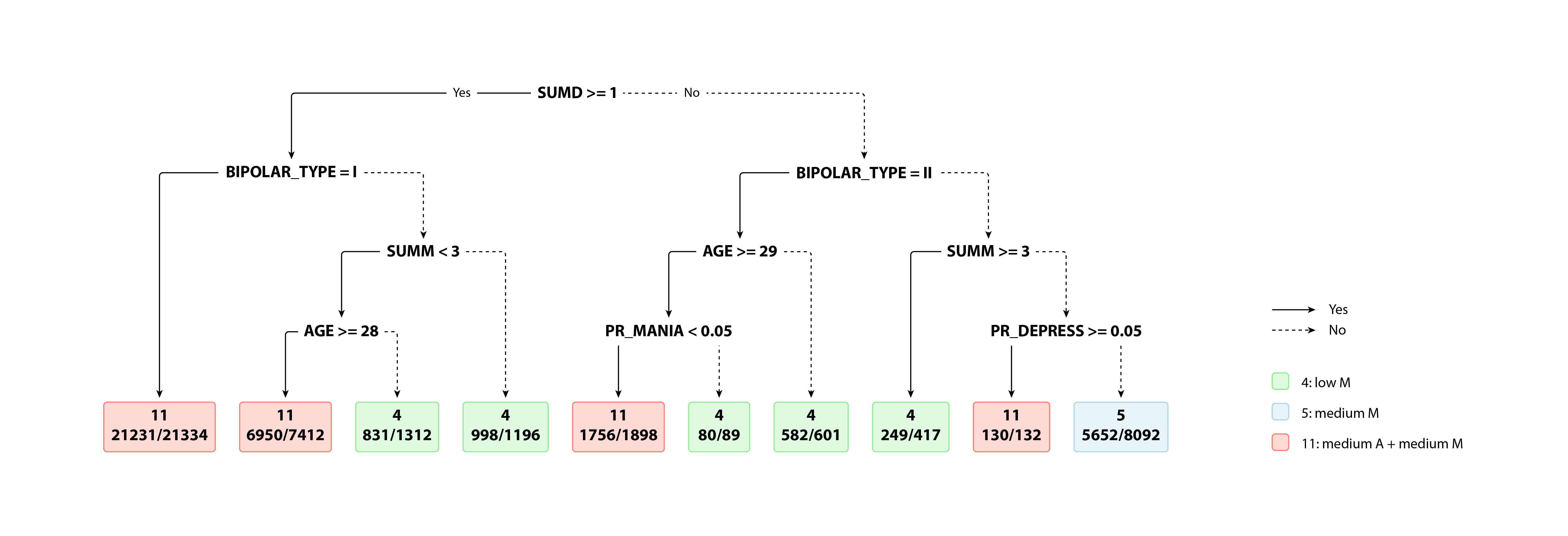
Figure 2: Estimated optimal treatment regime obtained by maximizing average utility, which is projected onto a decision tree for interpretation. Each tree node shows the splitting criterion, majority treatment label, and its proportion.

8 Conclusions

We developed a framework for estimation of an optimal treatment regime using data from long-term observational or randomized clinical studies. From a precision medicine perspective, a key contribution of this work is the incorporation of a patient’s latent health status, e.g., their true mood state in the context of bipolar depression. We showed that using this structure can lead to estimated optimal regimes that are clinically meaningful and that significantly outperform methods that fail to use this structure. From a methodological perspective, a key contribution is the development of methods for estimation and inference for the optimal treatment regime using from data generated from a POMDP. One could generalize the proposed methodology to include continuous latent processes. Such an approach is aligned with existing work in POMDPs in the computer science and engineering literature. We leave such extensions to future work.

Appendix I: Tables for medications

Medication name	Low dose (mg)	Medium dose (mg)	High dose (mg)
Deseryl	$<200$	$200-400$	$>400$
Serzone	$<200$	$200-400$	$>400$
Citalopram	$<20$	$20-40$	$>40$
Escitalopram Oxalate	$<10$	$10-20$	$>20$
Prozac	$<20$	$20-40$	$>40$
Fluvoxamine	$<100$	$100-200$	$>200$
Paroxetine	$<20$	$20-40$	$>40$
Zoloft	$<50$	$50-100$	$>100$
Venlafaxine	$<75$	$75-150$	$>150$
Bupropion	$<150$	$150-300$	$>300$

Table 8: List of common antidepressants in STEP-BD. The dose is divided into 3 levels: low, medium, and high.

Medication name	Low dose (mg)	Medium dose (mg)	High dose (mg)
Tegretol	$<400$	$400-800$	$>800$
Valproate	$<1000$	$1000-2000$	$>2000$
Olanzapine	$<10$	$10-20$	$>20$
Quetiapine	$<400$	$400-800$	$>800$
Clozapine	$<200$	$200-400$	$>400$
Lithium	$<900$	$900-1800$	$>1800$
Risperdal	$<2$	$2-4$	$>4$
Geodon	$<80$	$80-160$	$>160$
Abilify	$<15$	$15-30$	$>30$
Lamictal	$<100$	$100-200$	$>200$

Table 9: List of common mood stabilizers in STEP-BD. The dose is divided into 3 levels: low, medium, and high.

Appendix II: Estimated optimal treatment regime for total discounted utility

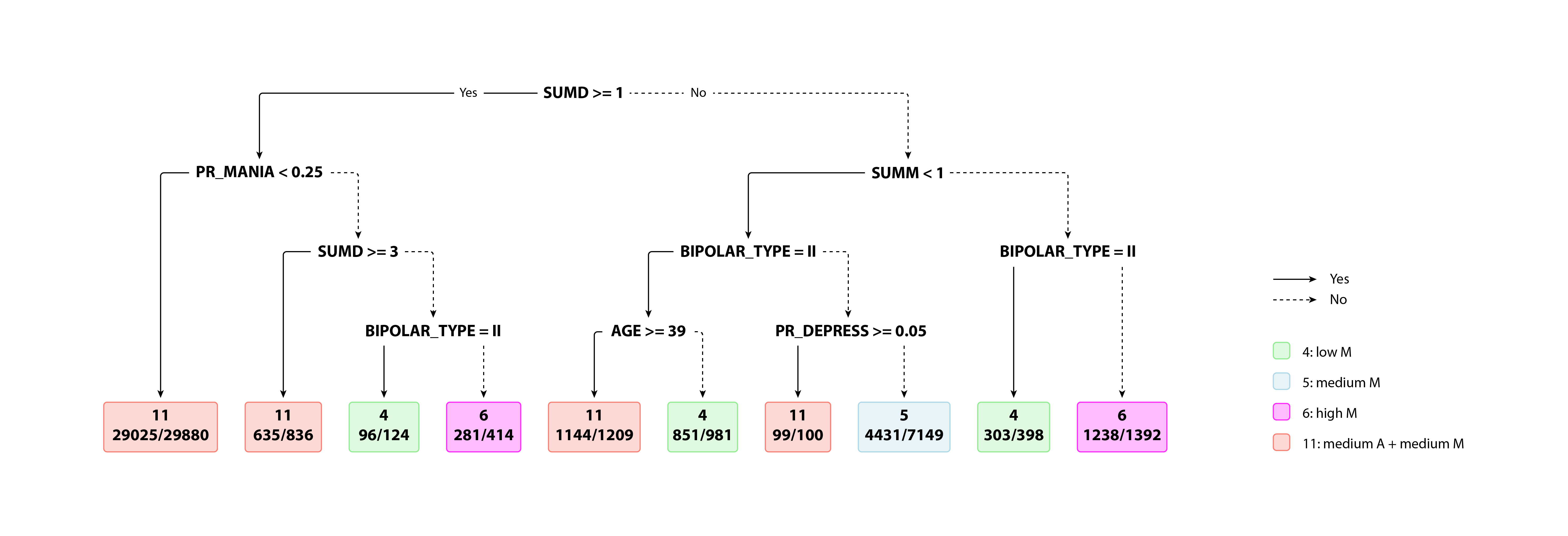
Figure 3: Estimate optimal treatment regime by maximizing total discounted utility ($\gamma=0.95$), which is projected onto a decision tree for interpretation. Each tree node shows the splitting criterion, majority treatment label and its proportion.

References

• Albert (1962) Albert, A. (1962). Estimating the infinitesimal generator of a continuous time, finite state markov process. The Annals of Mathematical Statistics, 727–753.
• Allman et al. (2009) Allman, E. S., C. Matias, J. A. Rhodes, et al. (2009). Identifiability of parameters in latent structure models with many observed variables. The Annals of Statistics 37(6A), 3099–3132.
• Athey and Imbens (2016) Athey, S. and G. Imbens (2016). Recursive partitioning for heterogeneous causal effects. Proceedings of the National Academy of Sciences 113(27), 7353–7360.
• Athreya and Lahiri (2006) Athreya, K. B. and S. N. Lahiri (2006). Measure theory and probability theory. Springer Science & Business Media.
• Berger and Boos (1994) Berger, R. L. and D. D. Boos (1994). P values maximized over a confidence set for the nuisance parameter. Journal of the American Statistical Association 89(427), 1012–1016.
• Bickel et al. (1998) Bickel, P. J., Y. Ritov, and T. Ryden (1998). Asymptotic normality of the maximum-likelihood estimator for general hidden markov models. The Annals of Statistics 26(4), 1614–1635.
• Bonsall et al. (2015) Bonsall, M. B., J. R. Geddes, G. M. Goodwin, and E. A. Holmes (2015). Bipolar disorder dynamics: affective instabilities, relaxation oscillations and noise. Journal of the Royal Society Interface 12(112), 20150670.
• Bonsall et al. (2011) Bonsall, M. B., S. M. Wallace-Hadrill, J. R. Geddes, G. M. Goodwin, and E. A. Holmes (2011). Nonlinear time-series approaches in characterizing mood stability and mood instability in bipolar disorder. Proceedings of the Royal Society B: Biological Sciences 279(1730), 916–924.
• Busoniu et al. (2017) Busoniu, L., R. Babuska, B. De Schutter, and D. Ernst (2017). Reinforcement learning and dynamic programming using function approximators. CRC press.
• Cassandra (1998) Cassandra, A. R. (1998). A survey of pomdp applications. In Working notes of AAAI 1998 fall symposium on planning with partially observable Markov decision processes, Volume 1724.
• Cavazos-Cadena (1988) Cavazos-Cadena, R. (1988). Necessary and sufficient conditions for a bounded solution to the optimality equation in average reward markov decision chains. Systems & control letters 10(1), 71–78.
• Chakraborty and Murphy (2014) Chakraborty, B. and S. A. Murphy (2014). Dynamic treatment regimes. Annual review of statistics and its application 1, 447–464.
• Ciarleglio et al. (2015) Ciarleglio, A., E. Petkova, R. T. Ogden, and T. Tarpey (2015). Treatment decisions based on scalar and functional baseline covariates. Biometrics 71(4), 884–894.
• Ciarleglio et al. (2016) Ciarleglio, A., E. Petkova, T. Tarpey, and R. T. Ogden (2016). Flexible functional regression methods for estimating individualized treatment rules. Stat 5(1), 185–199.
• Daugherty et al. (2009) Daugherty, D., T. Roque-Urrea, J. Urrea-Roque, J. Troyer, S. Wirkus, and M. A. Porter (2009). Mathematical models of bipolar disorder. Communications in Nonlinear Science and Numerical Simulation 14(7), 2897–2908.
• Douc and Matias (2001) Douc, R. and C. Matias (2001). Asymptotics of the maximum likelihood estimator for general hidden markov models. Bernoulli 7(3), 381–420.
• Douc et al. (2004) Douc, R., E. Moulines, and T. Rydén (2004). Asymptotic properties of the maximum likelihood estimator in autoregressive models with markov regime. The Annals of statistics 32(5), 2254–2304.
• Ertefaie (2019) Ertefaie, A. (2019). Constructing dynamic treatment regimes in infinite-horizon settings. arXiv preprint arXiv:1406.0764.
• Fedus et al. (2019) Fedus, W., C. Gelada, Y. Bengio, M. G. Bellemare, and H. Larochelle (2019). Hyperbolic discounting and learning over multiple horizons. arXiv preprint arXiv:1902.06865.
• Gassiat et al. (2013) Gassiat, E., A. Cleynen, and S. Robin (2013). Finite state space non parametric hidden markov models are in general identifiable. arXiv preprint arXiv:1306.4657.
• Hanna et al. (2018) Hanna, J. P., S. Niekum, and P. Stone (2018). Importance sampling policy evaluation with an estimated behavior policy. arXiv preprint arXiv:1806.01347.
• Hansen (1998) Hansen, E. A. (1998). Solving pomdps by searching in policy space. In Proceedings of the Fourteenth conference on Uncertainty in artificial intelligence, pp.  211–219. Morgan Kaufmann Publishers Inc.
• Henderson et al. (2010) Henderson, R., P. Ansell, and D. Alshibani (2010). Regret-regression for optimal dynamic treatment regimes. Biometrics 66(4), 1192–1201.
• Hernández-Lerma et al. (1991) Hernández-Lerma, O., R. Montes-de Oca, and R. Cavazos-Cadena (1991). Recurrence conditions for markov decision processes with borel state space: a survey. Annals of Operations Research 28(1), 29–46.
• Holmes et al. (2016) Holmes, E., M. Bonsall, S. Hales, H. Mitchell, F. Renner, S. Blackwell, P. Watson, G. Goodwin, and M. Di Simplicio (2016). Applications of time-series analysis to mood fluctuations in bipolar disorder to promote treatment innovation: a case series. Translational Psychiatry 6(1), e720.
• J Pineau (2003) J Pineau, G Gordon, S. T. (2003). Point-based value iteration: An anytime algorithm for pomdps. International Joint Conference on Artificial Intelligence.
• Jensen and Petersen (1999) Jensen, J. L. and N. V. Petersen (1999). Asymptotic normality of the maximum likelihood estimator in state space models. The Annals of Statistics 27(2), 514–535.
• Ji et al. (2007) Ji, S., R. Parr, H. Li, X. Liao, and L. Carin (2007). Point-based policy iteration. In AAAI, pp.  1243–1249.
• Jiang et al. (2019) Jiang, B., R. Song, J. Li, and D. Zeng (2019). Entropy learning for dynamic treatment regimes. Statistica Sinica.
• Jiang and Li (2015) Jiang, N. and L. Li (2015). Doubly robust off-policy value evaluation for reinforcement learning. arXiv preprint arXiv:1511.03722.
• Kaelbling et al. (1998) Kaelbling, L. P., M. L. Littman, and A. R. Cassandra (1998). Planning and acting in partially observable stochastic domains. Artificial intelligence 101(1-2), 99–134.
• Kosorok (2008) Kosorok, M. R. (2008). Introduction to empirical processes and semiparametric inference. Springer.
• Kurano (1986) Kurano, M. (1986). Markov decision processes with a borel measurable cost function?the average case. Mathematics of operations research 11(2), 309–320.
• Laber and Zhao (2015) Laber, E. and Y. Zhao (2015). Tree-based methods for individualized treatment regimes. Biometrika 102(3), 501–514.
• Laber et al. (2014) Laber, E. B., D. J. Lizotte, M. Qian, W. E. Pelham, and S. A. Murphy (2014). Dynamic treatment regimes: Technical challenges and applications. Electronic journal of statistics 8(1), 1225.
• Laber and Staicu (2017) Laber, E. B. and A.-M. Staicu (2017). Functional feature construction for individualized treatment regimes. Journal of the American Statistical Association (just-accepted).
• Le Gland and Mevel (2000) Le Gland, F. and L. Mevel (2000). Exponential forgetting and geometric ergodicity in hidden markov models. Mathematics of Control, Signals and Systems 13(1), 63–93.
• Leroux (1992) Leroux, B. G. (1992). Maximum-likelihood estimation for hidden markov models. Stochastic processes and their applications 40(1), 127–143.
• Liao et al. (2019) Liao, P., P. Klasnja, and S. Murphy (2019). Off-policy estimation of long-term average outcomes with applications to mobile health. arXiv preprint arXiv:1912.13088.
• Liu et al. (2019) Liu, N., Y. Liu, B. Logan, Z. Xu, J. Tang, and Y. Wang (2019). Learning the dynamic treatment regimes from medical registry data through deep q-network. Scientific reports 9(1), 1495.
• Liu et al. (2015) Liu, Y.-Y., S. Li, F. Li, L. Song, and J. M. Rehg (2015). Efficient learning of continuous-time hidden markov models for disease progression. In Advances in neural information processing systems, pp. 3600–3608.
• Lu et al. (2013) Lu, W., H. H. Zhang, and D. Zeng (2013). Variable selection for optimal treatment decision. Statistical methods in medical research 22(5), 493–504.
• Luckett et al. (2019) Luckett, D. J., E. B. Laber, A. R. Kahkoska, D. M. Maahs, E. Mayer-Davis, and M. R. Kosorok (2019). Estimating dynamic treatment regimes in mobile health using v-learning. Journal of the American Statistical Association, 1–34.
• Luedtke and van der Laan (2016) Luedtke, A. R. and M. J. van der Laan (2016). Super-learning of an optimal dynamic treatment rule. The international journal of biostatistics 12(1), 305–332.
• McKeague and Qian (2014) McKeague, I. W. and M. Qian (2014). Estimation of treatment policies based on functional predictors. Statistica Sinica 24(3), 1461.
• Meyn and Tweedie (2012) Meyn, S. P. and R. L. Tweedie (2012). Markov chains and stochastic stability. Springer Science & Business Media.
• Monahan (1982) Monahan, G. E. (1982). State of the art—a survey of partially observable markov decision processes: theory, models, and algorithms. Management Science 28(1), 1–16.
• Moodie et al. (2014) Moodie, E. E., N. Dean, and Y. R. Sun (2014). Q-learning: Flexible learning about useful utilities. Statistics in Biosciences 6(2), 223–243.
• Moodie et al. (2007) Moodie, E. E., T. S. Richardson, and D. A. Stephens (2007). Demystifying optimal dynamic treatment regimes. Biometrics 63(2), 447–455.
• Moore et al. (2012) Moore, P. J., M. A. Little, P. E. McSharry, J. R. Geddes, and G. M. Goodwin (2012). Forecasting depression in bipolar disorder. IEEE Transactions on Biomedical Engineering 59(10), 2801–2807.
• Moore et al. (2014) Moore, P. J., M. A. Little, P. E. McSharry, G. M. Goodwin, and J. R. Geddes (2014). Mood dynamics in bipolar disorder. International journal of bipolar disorders 2(1), 11.
• Murphy (2003) Murphy, S. A. (2003). Optimal dynamic treatment regimes. Journal of the Royal Statistical Society: Series B (Statistical Methodology) 65(2), 331–355.
• Murphy (2005) Murphy, S. A. (2005). A generalization error for q-learning. Journal of Machine Learning Research 6(Jul), 1073–1097.
• Murphy et al. (2016) Murphy, S. A., Y. Deng, E. B. Laber, H. R. Maei, R. S. Sutton, and K. Witkiewitz (2016). A batch, off-policy, actor-critic algorithm for optimizing the average reward. arXiv preprint arXiv:1607.05047.
• Murphy et al. (2001) Murphy, S. A., M. J. van der Laan, J. M. Robins, and C. P. P. R. Group (2001). Marginal mean models for dynamic regimes. Journal of the American Statistical Association 96(456), 1410–1423.
• Patel et al. (2015) Patel, R., P. Reiss, H. Shetty, M. Broadbent, R. Stewart, P. McGuire, and M. Taylor (2015). Do antidepressants increase the risk of mania and bipolar disorder in people with depression? a retrospective electronic case register cohort study. BMJ open 5(12), e008341.
• Powell (2007) Powell, W. B. (2007). Approximate Dynamic Programming: Solving the curses of dimensionality, Volume 703. John Wiley & Sons.
• Puterman (2014) Puterman, M. L. (2014). Markov decision processes: discrete stochastic dynamic programming. John Wiley & Sons.
• Pyke (1961a) Pyke, R. (1961a). Markov renewal processes: definitions and preliminary properties. The Annals of Mathematical Statistics, 1231–1242.
• Pyke (1961b) Pyke, R. (1961b). Markov renewal processes with finitely many states. The Annals of Mathematical Statistics, 1243–1259.
• Rabiner (1989) Rabiner, L. R. (1989). A tutorial on hidden markov models and selected applications in speech recognition. Proceedings of the IEEE 77(2), 257–286.
• Robins et al. (2008) Robins, J., L. Orellana, and A. Rotnitzky (2008). Estimation and extrapolation of optimal treatment and testing strategies. Statistics in medicine 27(23), 4678–4721.
• (63) Robins, J. M. Causal inference from complex longitudinal data.
• Robins (1999) Robins, J. M. (1999). Testing and estimation of direct effects by reparameterizing directed acyclic graphs with structural nested models. Computation, causation, and discovery, 349–405.
• Robins (2004) Robins, J. M. (2004). Optimal structural nested models for optimal sequential decisions. In Proceedings of the second seattle Symposium in Biostatistics, pp.  189–326. Springer.
• Rubin (2004) Rubin, D. B. (2004). Multiple imputation for nonresponse in surveys, Volume 81. John Wiley & Sons.
• Rubin and van der Laan (2012) Rubin, D. B. and M. J. van der Laan (2012). Statistical issues and limitations in personalized medicine research with clinical trials. The international journal of biostatistics 8(1).
• Sachs et al. (2003) Sachs, G. S., M. E. Thase, M. W. Otto, M. Bauer, D. Miklowitz, S. R. Wisniewski, P. Lavori, B. Lebowitz, M. Rudorfer, E. Frank, et al. (2003). Rationale, design, and methods of the systematic treatment enhancement program for bipolar disorder (step-bd). Biological psychiatry 53(11), 1028–1042.
• Schulte et al. (2014) Schulte, P. J., A. A. Tsiatis, E. B. Laber, and M. Davidian (2014). Q-and a-learning methods for estimating optimal dynamic treatment regimes. Statistical science: a review journal of the Institute of Mathematical Statistics 29(4), 640.
• Shi et al. (2018) Shi, C., A. Fan, R. Song, and W. Lu (2018). High-dimensional a-learning for optimal dynamic treatment regimes. Annals of statistics 46(3), 925–957.
• Shi et al. (2019) Shi, C., W. Lu, and R. Song (2019). A sparse random projection-based test for overall qualitative treatment effects. Journal of the American Statistical Association (just-accepted), 1–41.
• Song et al. (2015) Song, R., W. Wang, D. Zeng, and M. R. Kosorok (2015). Penalized q-learning for dynamic treatment regimens. Statistica Sinica 25(3), 901.
• Sutton et al. (2018) Sutton, R. S., A. G. Barto, et al. (2018). Reinforcement learning: An introduction. MIT press.
• Szepesvári (2010) Szepesvári, C. (2010). Algorithms for reinforcement learning. Synthesis lectures on artificial intelligence and machine learning 4(1), 1–103.
• Tao et al. (2018) Tao, Y., L. Wang, and D. Almirall (2018). Tree-based reinforcement learning for estimating optimal dynamic treatment regimes. The annals of applied statistics 12(3), 1914.
• Taylor et al. (2015) Taylor, J. M., W. Cheng, and J. C. Foster (2015). Reader reaction to “a robust method for estimating optimal treatment regimes” by zhang et al.(2012). Biometrics 71(1), 267–273.
• Tewari and Murphy (2017) Tewari, A. and S. A. Murphy (2017). From ads to interventions: Contextual bandits in mobile health. In Mobile Health, pp.  495–517. Springer.
• Thomas and Brunskill (2016) Thomas, P. and E. Brunskill (2016). Data-efficient off-policy policy evaluation for reinforcement learning. In International Conference on Machine Learning, pp. 2139–2148.
• Tian et al. (2014) Tian, L., A. A. Alizadeh, A. J. Gentles, and R. Tibshirani (2014). A simple method for estimating interactions between a treatment and a large number of covariates. Journal of the American Statistical Association 109(508), 1517–1532.
• Tsiatis et al. (2019) Tsiatis, A., M. Davidian, S. Holloway, and E. Laber (2019). Dynamic Treatment Regimes: Statistical Methods for Precision Medicine. CRC press.
• van der Laan (2006) van der Laan, M. J. (2006). Causal effect models for intention to treat and realistic individualized treatment rules.
• van der Vaart and Wellner (1996) van der Vaart, A. W. and J. A. Wellner (1996). Weak convergence. In Weak convergence and empirical processes, pp.  16–28. Springer.
• Wager and Athey (2018) Wager, S. and S. Athey (2018). Estimation and inference of heterogeneous treatment effects using random forests. Journal of the American Statistical Association 113(523), 1228–1242.
• Wallace et al. (2019) Wallace, M. P., E. E. Moodie, and D. A. Stephens (2019). Model selection for g-estimation of dynamic treatment regimes. Biometrics.
• Wiering and Van Otterlo (2012) Wiering, M. and M. Van Otterlo (2012). Reinforcement learning. Adaptation, learning, and optimization 12, 3.
• Wu et al. (2015) Wu, F., E. B. Laber, I. A. Lipkovich, and E. Severus (2015). Who will benefit from antidepressants in the acute treatment of bipolar depression? a reanalysis of the step-bd study by sachs et al. 2007, using q-learning. International journal of bipolar disorders 3(1), 7.
• Xu et al. (2016) Xu, Y., P. Müller, A. S. Wahed, and P. F. Thall (2016). Bayesian nonparametric estimation for dynamic treatment regimes with sequential transition times. Journal of the American Statistical Association 111(515), 921–950.
• Yamada (1975) Yamada, K. (1975). Duality theorem in markovian decision problems. Journal of mathematical analysis and applications 50(3), 579–595.
• Zhang et al. (2012) Zhang, B., A. A. Tsiatis, M. Davidian, M. Zhang, and E. Laber (2012). Estimating optimal treatment regimes from a classification perspective. Stat 1(1), 103–114.
• Zhang et al. (2018) Zhang, Y., E. B. Laber, M. Davidian, and A. A. Tsiatis (2018). Interpretable dynamic treatment regimes. Journal of the American Statistical Association 113(524), 1541–1549.
• Zhao et al. (2009) Zhao, Y., M. R. Kosorok, and D. Zeng (2009). Reinforcement learning design for cancer clinical trials. Statistics in medicine 28(26), 3294–3315.
• Zhao et al. (2012) Zhao, Y., D. Zeng, A. J. Rush, and M. R. Kosorok (2012). Estimating individualized treatment rules using outcome weighted learning. Journal of the American Statistical Association 107(499), 1106–1118.
• Zhao et al. (2015) Zhao, Y.-Q., D. Zeng, E. B. Laber, and M. R. Kosorok (2015). New statistical learning methods for estimating optimal dynamic treatment regimes. Journal of the American Statistical Association 110(510), 583–598.