Optimal Experimental Design for Infinite-dimensional Bayesian Inverse Problems Governed by PDEs: A Review

Abstract

We present a review of methods for optimal experimental design (OED) for Bayesian inverse problems governed by partial differential equations with infinite-dimensional parameters. The focus is on problems where one seeks to optimize the placement of measurement points, at which data are collected, such that the uncertainty in the estimated parameters is minimized. We present the mathematical foundations of OED in this context and survey the computational methods for the class of OED problems under study. We also outline some directions for future research in this area.

Keywords: optimal experimental design, inverse problem, Bayesian inference in Hilbert space, sensor placement.

1 Introduction

Mathematical models of complex physical and biological systems play a crucial role in understanding real world phenomena and making predictions. Examples include models of weather systems, ocean circulation, ice-sheet dynamics, porous media flow, or spread of infectious diseases. Models governing complex systems typically include a large number of parameters that are needed for a full model specification. Typically, some model parameters are uncertain and need to be estimated using indirect measurements. This is done by solving an inverse problem [41, 106, 103] that uses the model and measurement data to estimate the unknown parameters. Optimal experimental design (OED) [84, 8, 90, 104] comprises a critical component of parameter estimation; it provides a rigorous framework to guide acquisition of data, using limited resources, to construct model parameters with minimized uncertainty.

Models of complex systems are often described by systems of partial differential equations (PDEs). Also, in many applications, the unknown parameters to be estimated are functions, e.g., coefficient functions, initial states, or source terms. This review article is about OED for inverse problems governed by PDEs with infinite-dimensional inversion parameters. We focus on the Bayesian approach to inverse problems [103, 64, 101], which provides a comprehensive framework for quantification of uncertainties inherent to parameters and experimental data. In this approach, we use measurement data and a mathematical model to update the prior knowledge about unknown model parameters. The prior knowledge is encoded in a prior distribution law for the unknown parameters. The solution of a Bayesian inverse problem, known as the posterior distribution, is a distribution law of the unknown parameters which is consistent with measurement data, the model, and the prior distribution; see Figure 1.

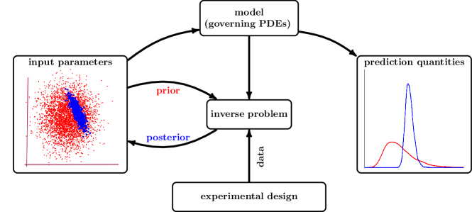
Figure 1: An overview of Bayesian approach to inverse problems. The Bayesian approach also enables making predictions with quantified and reduced uncertainties.

The study of the Bayesian approach to infinite-dimensional inverse problems traces back to the article [46]. Early follow up works include [78], [88], [73], and [45]. Significant progress has been made in this area in recent years; the references [72, 71, 101, 1, 52, 86, 38, 100] provide a small sample of literature from the last couple of decades. There has also been notable strides in computational methods for infinite-dimensional Bayesian inverse problems; see, e.g., [31, 50, 85, 62, 32, 15, 93, 98, 12].

The OED problem seeks an experimental design, guiding data acquisition, that minimizes the uncertainty in the estimated parameters. Making this precise requires a discussion of design criteria [26, 104]. There are various such criteria, which attempt to measure the uncertainty in the estimated parameters in different ways. For example, the so called A-optimal criterion quantifies the average variance of the estimated parameters.

Measurement data, needed in parameter estimation, can be costly or time consuming to acquire. This can put severe limits on the amount of experimental data that can be collected. In such cases, a naive or otherwise suboptimal experimental design entails waste of experimental resources and computing budget used to process the data, as well as possibly inaccurate parameter estimates. Even in cases when data acquisition is not very expensive, it is important to identify an optimal set of experiments. A suboptimal data acquisition strategy could lead to processing datasets with redundancies or, worse yet, one might miss important measurements leading to poor parameter estimation. In short, OED is a crucial aspect of successful parameter estimation and uncertainty quantification.

In Bayesian inversion and OED for infinite-dimensional inverse problems, it is important to consider the problem in a function space setting, before proceeding to discretization. Not only does this lead to rigorous formulations, it also is of practical importance when developing solution methods: this guides the choice of prior measures that are meaningful for infinite-dimensional parameters [101] and forces one to use appropriate discretizations of the Bayesian inverse problem. The latter is important because if the discretization of the various components of a Bayesian inverse problem is not performed correctly, the computed results will not converge to their infinite-dimensional counterparts upon grid refinements; see [21, 22]. Considering the problem in an infinite-dimensional setting also ensures definition of OED criteria that are meaningful in infinite dimensions. These criteria can then be discretized along with the Bayesian inverse problem. This way, the discretized OED criteria will have a meaningful infinite-dimensional limit upon successive grid refinements.

OED for infinite-dimensional inverse problems is challenging from both mathematical and computational points of view. The definition and analysis of OED criteria require tools from linear operator theory [91, 40] and probability theory on Hilbert spaces [87, 33]. Computationally, one is faced with optimization of expensive-to-evaluate (and differentiate) OED criteria. Note that the OED problem has the inverse problem as a sub-problem, which itself is an extremely challenging problem. These challenges are due to high-dimensionality of the inversion parameters, upon discretization, and high cost of simulating the governing model. Addressing the computational challenges of OED requires suitable approximations and computational methods that maximally exploit the problem structure within the inverse problem. These may include smoothing properties of the parameter-to-observable map or low-rank structures in operators appearing in the definition of OED criteria.

Broadly speaking, addressing mathematical and computational challenges of OED for infinite-dimensional Bayesian inverse problems governed by PDEs requires an interdisciplinary approach: the solution methods involve an intricate blend of methods and theories from mathematical and numerical analysis, inverse problem theory, numerical methods for PDEs, probability theory in function spaces, optimization, and uncertainty quantification. This article provides a review of this framework, for the class of OED problems under consideration. Our focus is primarily on situations where one seeks to optimize the locations of points where measurement data are collected. A prime example is the problem of optimal sensor placement.

A brief survey of literature. There is a rich body of literature devoted to OED for various classes of parameter estimation problems. Textbook references include [84, 8, 90, 104, 89, 43]. There are also a number of review articles on OED [26, 7, 29, 80, 95]. Here we present a non-exhaustive sample of the literature on OED for models governed by computationally intensive models.

Optimal design of experiments for inverse problems governed by ordinary differential equations or differential-algebraic equations appear in numerous works; examples include [13, 67, 11, 28, 17]. Recent works also include OED for inverse problems constrained by PDEs; see e.g., [57, 4, 42, 55, 108, 82, 25, 105]. Bayesian approaches to OED for nonlinear inverse problems governed by computationally challenging models were presented in [58, 59]; these articles use polynomial chaos expansions and Monte Carlo to estimate the OED objective, and use a stochastic optimization approach to compute the optimal design. The use of polynomial chaos surrogates makes this approach suitable for problems with low to moderate parameter dimensions. The articles [77, 76, 77] use Laplace approximations to efficiently compute the expected information gain, i.e., the D-optimal criterion, for nonlinear inverse problems. The article [107] presents an approach for OED with an alternate approach to statistical inverse problems in mind, known as the consistent Bayes approach [23]. The articles [3, 4, 2, 6] concern OED for infinite-dimensional Bayesian inverse problems. OED for infinite-dimensional problems is also treated in the PhD dissertation [108]. See also the PhD dissertation [53] that focuses on computational methods for design of infinite-dimensional Bayesian linear inverse problems. OED for large-scale problems has also been approached from a frequentist point of view. The articles [47, 48, 57, 49] provide excellent examples, where approaches based on Bayes risk minimization are presented. The article [94] uses a similar approach, but considers OED for inverse problems with state constraints. The utility of OED has been explored in a wide range of application areas involving large-scale inverse problems. Examples include seismic waveform inversion [39], electrical impedance tomography [61], borehole tomography [47], contaminant transport [3, 6] subsurface flow [4], natural gas networks [112], thermomechanics [55], iron loss in electrical machines [51], and forensic medicine [109].

Article overview. In Section 2, we present a few examples to motivate Bayesian inversion and OED for models governed by differential equations with infinite-dimensional parameters. Section 3 outlines some basics from probability theory and Bayesian inversion in Hilbert spaces. Theory and methods for design of Bayesian linear inverse problems are reviewed in Section 4. In that section, we also discuss a number of tools and techniques that will be needed for nonlinear inverse problems as well; these include definition of an experimental design, discretization issues, randomized matrix methods, and sparsity control. We discuss approaches for design of Bayesian nonlinear inverse problems in Section 5. In our discussion of the numerical methods for OED, we also point to references containing extensive computational results illustrating the effectiveness of the covered approaches. We conclude this review in Section 6 with closing remarks and several directions for future work.

2 Motivating Applications

In this section, we present several motivating applications to provide intuition on design of infinite-dimensional inverse problems governed by PDEs.

2.1 Contaminant source identification

In this example, we consider flow of a contaminant in a geological formation. The present example is adapted from [68]. Focusing on a horizontal cross-section of the medium, we consider a two dimensional domain $\mathcal{D}=[0,L_{1}]\times[0,L_{2}]$. The space-time evolution of the contaminant concentration, denoted by $u({\mathchoice{\mbox{\boldmath$\displaystyle{x}$}}{\mbox{\boldmath$\textstyle{x}$}}{\mbox{\boldmath$\scriptstyle{x}$}}{\mbox{\boldmath$\scriptscriptstyle{x}$}}},t)$, can be modeled by a time-dependent advection-diffusion equation:

$$\frac{\partial u}{\partial t}-\kappa\Delta{u}+\nabla\cdot({\mathchoice{\mbox{\boldmath$\displaystyle{v}$}}{\mbox{\boldmath$\textstyle{v}$}}{\mbox{\boldmath$\scriptstyle{v}$}}{\mbox{\boldmath$\scriptscriptstyle{v}$}}}\,u) =0\hskip 8.53581pt \mbox{ in }\mathcal{D}\times(0,T),$$ (1)

$$u(\cdot,0) =m\hskip 8.53581pt \mbox{ in }\mathcal{D},$$

$$(-\kappa\nabla{u}+u\,{\mathchoice{\mbox{\boldmath$\displaystyle{v}$}}{\mbox{\boldmath$\textstyle{v}$}}{\mbox{\boldmath$\scriptstyle{v}$}}{\mbox{\boldmath$\scriptscriptstyle{v}$}}})\cdot{\mathchoice{\mbox{\boldmath$\displaystyle{n}$}}{\mbox{\boldmath$\textstyle{n}$}}{\mbox{\boldmath$\scriptstyle{n}$}}{\mbox{\boldmath$\scriptscriptstyle{n}$}}} =0\hskip 8.53581pt \mbox{ in }\Gamma_{\!l}\times(0,T),$$

$$\kappa\nabla{u}\cdot{\mathchoice{\mbox{\boldmath$\displaystyle{n}$}}{\mbox{\boldmath$\textstyle{n}$}}{\mbox{\boldmath$\scriptstyle{n}$}}{\mbox{\boldmath$\scriptscriptstyle{n}$}}} =0\hskip 8.53581pt \mbox{ in }\partial\mathcal{D}\setminus\Gamma_{\!l}\times(0,T).$$

In the above problem, $\kappa>0$ is the diffusion coefficient, $\textstyle{v}$ is the velocity field, $T$ is the final time, and $m({\mathchoice{\mbox{\boldmath$\displaystyle{x}$}}{\mbox{\boldmath$\textstyle{x}$}}{\mbox{\boldmath$\scriptstyle{x}$}}{\mbox{\boldmath$\scriptscriptstyle{x}$}}})$ is the initial concentration field. We have denoted the left edge of the domain by $\Gamma_{\!l}$ and assume this part of $\partial\mathcal{D}$ is impermeable, as modeled by the zero total flux condition. The homogeneous pure Neumann condition on the rest of the boundary allows for advective flux. See [68], for more details on this model problem.

In the present example, sensor measurements of the concentration are used to estimate the initial concentration field $m({\mathchoice{\mbox{\boldmath$\displaystyle{x}$}}{\mbox{\boldmath$\textstyle{x}$}}{\mbox{\boldmath$\scriptstyle{x}$}}{\mbox{\boldmath$\scriptscriptstyle{x}$}}})$. This is an example of a linear inverse problem, because the measurement data is a linear function of the parameter $m$. The OED problem here seeks to specify the sensor locations so as to optimize the statistical quality of the estimated initial concentration field.

2.2 Permeability inversion in porous medium flow

We consider the problem of estimating the permeability field of a porous subsurface environment. We assume that a tracer substance flows through the domain. Again, we focus on a two-dimensional geometry and let domain $\mathcal{D}$ be the unit square. We denote by $\Gamma_{0}$, $\Gamma_{1}$, $\Gamma_{2}$, and $\Gamma_{3}$ the bottom, right, top, and left edges of the domain, respectively.

The following equations model the flow of the tracer through a medium that is saturated with a fluid:

$$-\nabla\cdot(e^{m}\nabla p) =0\quad\text{ in }\mathcal{D},$$ (2a)

$$\frac{\partial u}{\partial t}-\nabla\cdot\big{(}\kappa\nabla u\big{)}+\nabla\cdot\big{(}{\mathchoice{\mbox{\boldmath$\displaystyle{v}$}}{\mbox{\boldmath$\textstyle{v}$}}{\mbox{\boldmath$\scriptstyle{v}$}}{\mbox{\boldmath$\scriptscriptstyle{v}$}}}\,u\big{)} =g\quad\text{ in }[0,T]\times\mathcal{D},$$ (2b)

$$p =p_{1}\quad\text{on }\Gamma_{1},$$ (2c)

$$p =p_{2}\quad\text{on }\Gamma_{3},$$ (2d)

$$e^{m}\nabla p\cdot{\mathchoice{\mbox{\boldmath$\displaystyle{n}$}}{\mbox{\boldmath$\textstyle{n}$}}{\mbox{\boldmath$\scriptstyle{n}$}}{\mbox{\boldmath$\scriptscriptstyle{n}$}}} =0\quad\text{ on }\Gamma_{0}\cup\Gamma_{2},$$ (2e)

$$\nabla u\cdot{\mathchoice{\mbox{\boldmath$\displaystyle{n}$}}{\mbox{\boldmath$\textstyle{n}$}}{\mbox{\boldmath$\scriptstyle{n}$}}{\mbox{\boldmath$\scriptscriptstyle{n}$}}} =0\quad\text{ on }[0,T]\times\{\Gamma_{0}\cup\Gamma_{1}\cup\Gamma_{2}\cup\Gamma_{3}\},$$ (2f)

$$u(0,\cdot) =0\quad\text{ in }\mathcal{D}.$$ (2g)

Here $p$ denotes the pressure field (of the saturating fluid), $m$ is the log-permeability field of the medium, ${\mathchoice{\mbox{\boldmath$\displaystyle{v}$}}{\mbox{\boldmath$\textstyle{v}$}}{\mbox{\boldmath$\scriptstyle{v}$}}{\mbox{\boldmath$\scriptscriptstyle{v}$}}}=-e^{m}\nabla p$ the Darcy velocity, $u(t,{\mathchoice{\mbox{\boldmath$\displaystyle{x}$}}{\mbox{\boldmath$\textstyle{x}$}}{\mbox{\boldmath$\scriptstyle{x}$}}{\mbox{\boldmath$\scriptscriptstyle{x}$}}})$ is the tracer concentration, $\kappa$ is the diffusion constant, and $g$ is a source term. The Dirichlet pressure boundary conditions drive the flow. See [102], from which this example is taken, for more details.

In this example, we use sensor measurements of pressure and concentration to estimate the log-permeability field $m({\mathchoice{\mbox{\boldmath$\displaystyle{x}$}}{\mbox{\boldmath$\textstyle{x}$}}{\mbox{\boldmath$\scriptstyle{x}$}}{\mbox{\boldmath$\scriptscriptstyle{x}$}}})$. This is a nonlinear inverse problem; the function that maps the inversion parameter $m$ to the measurements is nonlinear. The OED problem here seeks to optimally place sensors that record concentration or pressure measurements.

2.3 Fault slip reconstruction in an earthquake

This problem, which is motivated by earthquake modeling, concerns the reconstruction of the fault slip, during an earthquake. The model problem here is adapted from [79, Chapter 2]. The 2D domain depicted in Figure 2 is a cross-section of an idealized geometry modeling a subduction zone. We represent the boundary of the domain $\mathcal{D}$ as $\partial\mathcal{D}=\Gamma_{b}\cup\Gamma_{t}\cup\Gamma_{s}$; see Figure 2.

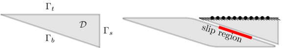
Figure 2: Model geometry in fault slip reconstruction inverse problem. Left: the computational domain. Right: idealized geometry depicting a subduction zone; the GPS stations on the top boundary of the domain record displacement during an earthquake.

The interest here is on estimating the slip along $\Gamma_{b}$ based on point measurements of elastic displacement on $\Gamma_{t}$.

Assuming a linear elastic equation for the displacement ${\mathchoice{\mbox{\boldmath$\displaystyle{u}$}}{\mbox{\boldmath$\textstyle{u}$}}{\mbox{\boldmath$\scriptstyle{u}$}}{\mbox{\boldmath$\scriptscriptstyle{u}$}}}=[\begin{matrix}u_{1}&\!u_{2}\end{matrix}]^{\mkern-1.5mu\mathsf{T}}$, we consider the governing model:

$$-\nabla\cdot{\mathchoice{\mbox{\boldmath$\displaystyle{\sigma}$}}{\mbox{\boldmath$\textstyle{\sigma}$}}{\mbox{\boldmath$\scriptstyle{\sigma}$}}{\mbox{\boldmath$\scriptscriptstyle{\sigma}$}}}({\mathchoice{\mbox{\boldmath$\displaystyle{u}$}}{\mbox{\boldmath$\textstyle{u}$}}{\mbox{\boldmath$\scriptstyle{u}$}}{\mbox{\boldmath$\scriptscriptstyle{u}$}}})={\mathchoice{\mbox{\boldmath$\displaystyle{0}$}}{\mbox{\boldmath$\textstyle{0}$}}{\mbox{\boldmath$\scriptstyle{0}$}}{\mbox{\boldmath$\scriptscriptstyle{0}$}}},\quad\text{in }\mathcal{D},$$

where $\sigma({\mathchoice{\mbox{\boldmath$\displaystyle{u}$}}{\mbox{\boldmath$\textstyle{u}$}}{\mbox{\boldmath$\scriptstyle{u}$}}{\mbox{\boldmath$\scriptscriptstyle{u}$}}})=\mu\,[\nabla{\mathchoice{\mbox{\boldmath$\displaystyle{u}$}}{\mbox{\boldmath$\textstyle{u}$}}{\mbox{\boldmath$\scriptstyle{u}$}}{\mbox{\boldmath$\scriptscriptstyle{u}$}}}+(\nabla{\mathchoice{\mbox{\boldmath$\displaystyle{u}$}}{\mbox{\boldmath$\textstyle{u}$}}{\mbox{\boldmath$\scriptstyle{u}$}}{\mbox{\boldmath$\scriptscriptstyle{u}$}}})^{\mkern-1.5mu\mathsf{T}}]+\lambda\nabla\cdot{\mathchoice{\mbox{\boldmath$\displaystyle{u}$}}{\mbox{\boldmath$\textstyle{u}$}}{\mbox{\boldmath$\scriptstyle{u}$}}{\mbox{\boldmath$\scriptscriptstyle{u}$}}}\mathbf{{I}}$, with $\mu$ and $\lambda$ denoting the Láme moduli. The boundary conditions are:

$${\mathchoice{\mbox{\boldmath$\displaystyle{\sigma}$}}{\mbox{\boldmath$\textstyle{\sigma}$}}{\mbox{\boldmath$\scriptstyle{\sigma}$}}{\mbox{\boldmath$\scriptscriptstyle{\sigma}$}}}({\mathchoice{\mbox{\boldmath$\displaystyle{u}$}}{\mbox{\boldmath$\textstyle{u}$}}{\mbox{\boldmath$\scriptstyle{u}$}}{\mbox{\boldmath$\scriptscriptstyle{u}$}}}){\mathchoice{\mbox{\boldmath$\displaystyle{n}$}}{\mbox{\boldmath$\textstyle{n}$}}{\mbox{\boldmath$\scriptstyle{n}$}}{\mbox{\boldmath$\scriptscriptstyle{n}$}}} =0\quad\text{ on }\Gamma_{t},$$

$${u} =0\quad\text{ on }\Gamma_{s},$$

$${\mathchoice{\mbox{\boldmath$\displaystyle{u}$}}{\mbox{\boldmath$\textstyle{u}$}}{\mbox{\boldmath$\scriptstyle{u}$}}{\mbox{\boldmath$\scriptscriptstyle{u}$}}}\cdot{\mathchoice{\mbox{\boldmath$\displaystyle{n}$}}{\mbox{\boldmath$\textstyle{n}$}}{\mbox{\boldmath$\scriptstyle{n}$}}{\mbox{\boldmath$\scriptscriptstyle{n}$}}} =0\quad\text{ on }\Gamma_{b},$$

$$\delta\mathbf{{T}}({\mathchoice{\mbox{\boldmath$\displaystyle{\sigma}$}}{\mbox{\boldmath$\textstyle{\sigma}$}}{\mbox{\boldmath$\scriptstyle{\sigma}$}}{\mbox{\boldmath$\scriptscriptstyle{\sigma}$}}}({\mathchoice{\mbox{\boldmath$\displaystyle{u}$}}{\mbox{\boldmath$\textstyle{u}$}}{\mbox{\boldmath$\scriptstyle{u}$}}{\mbox{\boldmath$\scriptscriptstyle{u}$}}}){\mathchoice{\mbox{\boldmath$\displaystyle{n}$}}{\mbox{\boldmath$\textstyle{n}$}}{\mbox{\boldmath$\scriptstyle{n}$}}{\mbox{\boldmath$\scriptscriptstyle{n}$}}})+\mathbf{{T}}{\mathchoice{\mbox{\boldmath$\displaystyle{u}$}}{\mbox{\boldmath$\textstyle{u}$}}{\mbox{\boldmath$\scriptstyle{u}$}}{\mbox{\boldmath$\scriptscriptstyle{u}$}}} ={\mathchoice{\mbox{\boldmath$\displaystyle{m}$}}{\mbox{\boldmath$\textstyle{m}$}}{\mbox{\boldmath$\scriptstyle{m}$}}{\mbox{\boldmath$\scriptscriptstyle{m}$}}}\quad\!\text{on }\Gamma_{b}.$$

Here $\textstyle{m}$ is the inversion parameter, $\delta>0$, and $\mathbf{{T}}$ is the tangential operator that extracts the tangential components of a vector; i.e., $\mathbf{{T}}{\mathchoice{\mbox{\boldmath$\displaystyle{u}$}}{\mbox{\boldmath$\textstyle{u}$}}{\mbox{\boldmath$\scriptstyle{u}$}}{\mbox{\boldmath$\scriptscriptstyle{u}$}}}\vcentcolon=(\mathbf{{I}}-{\mathchoice{\mbox{\boldmath$\displaystyle{n}$}}{\mbox{\boldmath$\textstyle{n}$}}{\mbox{\boldmath$\scriptstyle{n}$}}{\mbox{\boldmath$\scriptscriptstyle{n}$}}}\otimes{\mathchoice{\mbox{\boldmath$\displaystyle{n}$}}{\mbox{\boldmath$\textstyle{n}$}}{\mbox{\boldmath$\scriptstyle{n}$}}{\mbox{\boldmath$\scriptscriptstyle{n}$}}}){\mathchoice{\mbox{\boldmath$\displaystyle{u}$}}{\mbox{\boldmath$\textstyle{u}$}}{\mbox{\boldmath$\scriptstyle{u}$}}{\mbox{\boldmath$\scriptscriptstyle{u}$}}}={\mathchoice{\mbox{\boldmath$\displaystyle{u}$}}{\mbox{\boldmath$\textstyle{u}$}}{\mbox{\boldmath$\scriptstyle{u}$}}{\mbox{\boldmath$\scriptscriptstyle{u}$}}}-({\mathchoice{\mbox{\boldmath$\displaystyle{n}$}}{\mbox{\boldmath$\textstyle{n}$}}{\mbox{\boldmath$\scriptstyle{n}$}}{\mbox{\boldmath$\scriptscriptstyle{n}$}}}^{\mkern-1.5mu\mathsf{T}}{\mathchoice{\mbox{\boldmath$\displaystyle{u}$}}{\mbox{\boldmath$\textstyle{u}$}}{\mbox{\boldmath$\scriptstyle{u}$}}{\mbox{\boldmath$\scriptscriptstyle{u}$}}}){\mathchoice{\mbox{\boldmath$\displaystyle{n}$}}{\mbox{\boldmath$\textstyle{n}$}}{\mbox{\boldmath$\scriptstyle{n}$}}{\mbox{\boldmath$\scriptscriptstyle{n}$}}}$, where $\textstyle{n}$ is the outward pointing unit normal on the boundary.

In this example, the inverse problem seeks to estimate $\textstyle{m}$ using displacement measurements at the top boundary. This is another example of a linear inverse problem. The OED problem here aims to optimally place the GPS stations that take displacement measurements on $\Gamma_{t}$.

2.4 Parameter inversion in an epidemic model

While our focus is on inverse problems governed by PDEs, we also present an example where the governing model is a system of ordinary differential equations. Specifically, we consider a compartment model of the spread of a disease known as the SEIRD model; see e.g., [20] for more details on such models. This model tracks the populations of susceptible, exposed, infected, recovered, and dead individuals. The governing model can be written as

$$S^{\prime} =-\beta SI/N,$$

$$E^{\prime} =\phantom{-}\beta SI/N-\sigma E,$$

$$I^{\prime} =\phantom{-}\sigma E-(\gamma+\delta)I,$$

$$R^{\prime} =\phantom{-}\gamma I,$$

$$D^{\prime} =\phantom{-}\delta I.$$

Here $N=S+E+I+R+D$ and $\beta$, $\sigma$, $\gamma$, and $\delta$ are, respectively, the rates of disease transmission, progression from exposed to infected, recovery, and disease-related mortality. The parameters $\sigma$, $\gamma$, and $\delta$ are scalars that depend on the specific disease. However, $\beta$ is influenced by the contact rate between individuals of a given population, which can change over time. This can be, for example, as a result of social distancing policies that reduce contact rate among individuals. Therefore, in general $\beta$ is a function of time. The inversion parameters here include the infinite-dimensional parameter $\beta(t)$ and the scalar parameters $\sigma$, $\gamma$, and $\delta$.

The inverse problem here seeks to estimate the unknown parameters using observations of infected people at a number of observation times. An OED problem aims at finding optimal observation times. Of course, in this inverse problem one typically uses whatever data becomes available. In this case, OED is useful as it informs which measurement times are important for reliable parameter estimation. If the available datasets are missing data from key observation times, a practitioner would know a priori that parameter estimation is subject to large uncertainties.

3 Infinite-dimensional Bayesian inverse problems

In this section, we outline background materials regarding Bayesian inversion in an infinite-dimensional Hilbert space setting. We first discuss the requisite concepts regarding linear operators (Section 3.1) and probability measures (Section 3.2) on infinite-dimensional Hilbert spaces. Then, we sketch the Bayesian formulation of an inverse problem in a Hilbert space in Section 3.3. For more details on the theoretical foundations of Bayesian inversion in infinite dimensions and surveys of the related literature, we refer the readers to [101, 38].

3.1 Positive self-adjoint trace-class operators

Let $\mathscr{H}$ be an infinite-dimensional separable real Hilbert space equipped with inner product ${\left\langle{\cdot\,},{\cdot}\right\rangle}$ and the corresponding induced norm $\|\cdot\|={\left\langle{\cdot\,},{\cdot}\right\rangle}^{1/2}$. A bounded linear operator $\mathcal{A}:\mathscr{H}\to\mathscr{H}$ is called selfadjoint if ${\left\langle{\mathcal{A}u},{v}\right\rangle}={\left\langle{u},{\mathcal{A}v}\right\rangle}$ for all $u,v\in\mathscr{H}$. We call $\mathcal{A}$ positive if ${\left\langle{\mathcal{A}u},{u}\right\rangle}\geq 0$ for all $u\in\mathscr{H}$ and strictly positive if ${\left\langle{\mathcal{A}u},{u}\right\rangle}>0$ for all nonzero $u\in\mathscr{H}$. A positive selfadjoint bounded linear operator $\mathcal{A}$ on $\mathscr{H}$ is called of trace-class if

$$\mathsf{tr}(\mathcal{A})\vcentcolon=\sum_{k=1}^{\infty}{\left\langle{\mathcal{A}e_{k}},{e_{k}}\right\rangle}<\infty,$$ (3)

where $\{e_{k}\}_{k=1}^{\infty}$ is an orthonormal basis of $\mathscr{H}$. As is well-known [91, 30], the value of the summation in (3) does not depend on the choice of the orthonormal basis. Note also that if $\mathcal{A}$ is positive selfadjoint and of trace-class, then it has an orthonormal basis of eigenvectors $\{v_{k}\}_{k=1}^{\infty}$ with corresponding (real, non-negative) eigenvalues $\{\lambda_{k}\}_{k=1}^{\infty}$, and $\mathsf{tr}(\mathcal{A})=\sum_{k=1}^{\infty}{\left\langle{\mathcal{A}v_{k}},{v_{k}}\right\rangle}=\sum_{k=1}^{\infty}\lambda_{k}$.

3.2 Probability measures on a Hilbert space

Here we recall some basics regarding probability measures on Hilbert spaces.

Borel probability measures. We let $\mathscr{B}(\mathscr{H})$ denote the Borel $\sigma$-algebra on $\mathscr{H}$. A Borel probability measure on $\mathscr{H}$ is a probability measure on the measurable space $(\mathscr{H},\mathscr{B}(\mathscr{H}))$. Let $\mu$ be a Borel probability measure on $\mathscr{H}$ that has finite first and second moments. That is, $\int_{\mathscr{H}}\|z\|\,\mu(dz)<\infty$ and $\int_{\mathscr{H}}\|z\|^{2}\,\mu(dz)<\infty$. The mean $\bar{m}$ of $\mu$ is an element of $\mathscr{H}$ that satisfies

$${\left\langle{\bar{m}},{a}\right\rangle}=\int_{\mathscr{H}}{\left\langle{z},{a}\right\rangle}\,\mu(dz),\quad\text{for all }a\in\mathscr{H}.$$

The covariance operator of $\mu$ is a bounded linear operator $\mathcal{C}:\mathscr{H}\to\mathscr{H}$ that is characterized as follows:

$${\left\langle{\mathcal{C}a},{b}\right\rangle}=\int_{\mathscr{H}}{\left\langle{a},{z-\bar{m}}\right\rangle}{\left\langle{b},{z-\bar{m}}\right\rangle}\,\mu(dz),\quad a,b\in\mathscr{H}.$$

Note that $\mathcal{C}$ is positive and selfadjoint; it is also straightforward to show that $\mathcal{C}$ is of trace-class, as seen from the following standard argument [33]. Let $\{e_{k}\}_{k=1}^{\infty}$ be a complete orthonormal set in $\mathscr{H}$. We have

$$\mathsf{tr}(\mathcal{C})=\sum_{k=1}^{\infty}{\left\langle{\mathcal{C}e_{k}},{e_{k}}\right\rangle} =\sum_{k=1}^{\infty}\int_{\mathscr{H}}{\left\langle{e_{k}},{z-\bar{m}}\right\rangle}^{2}\,\mu(dz)$$ (4)

$$=\int_{\mathscr{H}}\sum_{k=1}^{\infty}{\left\langle{e_{k}},{z-\bar{m}}\right\rangle}^{2}\,\mu(dz)=\int_{\mathscr{H}}\|z-\bar{m}\|^{2}\,\mu(dz)<\infty,$$

where the interchange of the summation and the integral is justified by the Lebesgue Monotone Convergence Theorem and the final equality is due to Parseval’s identity.

We also recall that a Borel probability measure on $\mu$ on $(\mathscr{H},\mathscr{B}(\mathscr{H}))$ is uniquely characterized by its Fourier transform [33, Proposition 1.7], which is defined by

$$\hat{\mu}(\xi)\vcentcolon=\int_{\mathscr{H}}e^{i\langle{x},{\xi}\rangle}\,\mu(dx),\quad\xi\in\mathscr{H}.$$

Gaussian measures. An important class of probability measures encountered in Bayesian analysis in function spaces is that of Gaussian measures. We recall that $\mu$ is a Gaussian measure on $(\mathscr{H},\mathscr{B}(\mathscr{H}))$ if for every $x\in\mathscr{H}$ the linear functional $\ell(z)={\left\langle{x},{z}\right\rangle}$, considered as random variable $\ell:(\mathscr{H},\mathscr{B}(\mathscr{H}),\mu)\to(\mathbb{R},\mathscr{B}(\mathbb{R}))$, is a Gaussian random variable [35]. Gaussian measures on $\mathbb{R}^{n}$ that have strictly positive covariance operators can be characterized by the associated probability density function (PDF). This PDF is none but the Radon–Nikodym derivative [110] of the measure with the respect to the Lebesgue measure on $\mathbb{R}^{n}$. However, in the infinite-dimensional Hilbert space setting, there is no analogue of Lebesgue measure [33]. In this case, we can characterize a Gaussian measure using its Fourier transform. Namely, given $\bar{m}\in\mathscr{H}$ and a positive selfadjoint trace-class operator $\mathcal{C}$ on $\mathscr{H}$, the Gaussian measure $\mu=\mathcal{N}\!\left({\bar{m}},{\mathcal{C}}\right)$ is the unique probability measure with,

$$\hat{\mu}(\xi)=\exp\Big{\{}i\langle\bar{m},\xi\rangle-\frac{1}{2}\langle Q\xi,\xi\rangle\Big{\}},\quad\xi\in\mathscr{H}.$$

For further details regarding Gaussian measures on Hilbert spaces, see e.g.,[34, 33, 35]. See also [18], for a comprehensive treatment of Gaussian measures on Banach spaces.

Kullback-Leibler divergence. The Kullback-Leibler (KL) divergence provides a “measure of distance” between two probability measures [70]. Note that the KL divergence is not a metric, because it is non-symmetric and does not satisfy the triangle inequality. However, given probability measures $\mu_{1}$ and $\mu_{2}$, the KL divergence from $\mu_{1}$ to $\mu_{2}$ is non-negative and is zero if and only if the two measures are the same. As discussed in Section 4.1, in Bayesian OED, the KL divergence is used to define a notion of information gain.

For probability measures on $\mathbb{R}^{n}$ that admit densities (i.e., PDFs) with respect to the Lebesgue measure, we can define the KL divergence in terms of the densities. That is, if $\mu_{1}$ and $\mu_{2}$ are probability measures with densities $\pi_{1}$ and $\pi_{2}$, respectively, the KL divergence from $\mu_{1}$ to $\mu_{2}$, denoted by $D_{\text{kl}}\left({\mu_{1}}\|{\mu_{2}}\right)$, is given by

$$D_{\text{kl}}\left({\mu_{1}}\|{\mu_{2}}\right)=\int_{\mathbb{R}^{n}}\log\Big{\{}\frac{\pi_{1}({\mathchoice{\mbox{\boldmath$\displaystyle{x}$}}{\mbox{\boldmath$\textstyle{x}$}}{\mbox{\boldmath$\scriptstyle{x}$}}{\mbox{\boldmath$\scriptscriptstyle{x}$}}})}{\pi_{2}({\mathchoice{\mbox{\boldmath$\displaystyle{x}$}}{\mbox{\boldmath$\textstyle{x}$}}{\mbox{\boldmath$\scriptstyle{x}$}}{\mbox{\boldmath$\scriptscriptstyle{x}$}}})}\Big{\}}\,\pi_{1}({\mathchoice{\mbox{\boldmath$\displaystyle{x}$}}{\mbox{\boldmath$\textstyle{x}$}}{\mbox{\boldmath$\scriptstyle{x}$}}{\mbox{\boldmath$\scriptscriptstyle{x}$}}})\,d{\mathchoice{\mbox{\boldmath$\displaystyle{x}$}}{\mbox{\boldmath$\textstyle{x}$}}{\mbox{\boldmath$\scriptstyle{x}$}}{\mbox{\boldmath$\scriptscriptstyle{x}$}}}.$$

However, in an infinite-dimensional Hilbert space, where there is no analogue of the Lebesgue measure, we need to work with an abstract definition of KL divergence, which we explain next. Let $\mu_{1}$ and $\mu_{2}$ be two Borel probability measures on $\mathscr{H}$ and suppose $\mu_{1}$ is absolutely continuous with respect to $\mu_{2}$. The KL divergence from $\mu_{1}$ to $\mu_{2}$ is defined as

$$D_{\text{kl}}\left({\mu_{1}}\|{\mu_{2}}\right)=\int\log\Big{\{}\frac{d\mu_{1}}{d\mu_{2}}\Big{\}}\,d\mu_{1},$$

where $\frac{d\mu_{1}}{d\mu_{2}}$ is the Radon-Nikodym derivative of $\mu_{1}$ with respect to $\mu_{2}$. In the case that $\mu_{1}$ is not absolutely continuous with respect to $\mu_{2}$, we have $D_{\text{kl}}\left({\mu_{1}}\|{\mu_{2}}\right)=+\infty$.

$\mathscr{H}$-valued Random variables. Let $(\Omega,\Sigma,\mathbb{P})$ be a probability space [110] and let $m:(\Omega,\Sigma,\mathbb{P})\to(\mathscr{H},\mathscr{B}(\mathscr{H}))$ be a random variable. The law $\mu$ of $m$ is a probability measure on $(\mathscr{H},\mathscr{B}(\mathscr{H}))$ that satisfies,

$$\mu(E)=\mathbb{P}(m\in E)=\mathbb{P}(\{\omega\in\Omega:m(\omega)\in E\}),\quad\text{ for }E\in\mathscr{B}(\mathscr{H}).$$

In this article, we assume $\mathscr{H}=L^{2}(\mathcal{D})$ where $\mathcal{D}$ a bounded spatial domain that has a sufficiently regular boundary. (We can also consider the case where $\mathcal{D}$ is a time interval.) The inner product on $\mathscr{H}$ is the standard $L^{2}$ inner product. In this case, for each $\omega\in\Omega$, $m(\cdot,\omega)$ is a real-valued function on $\mathcal{D}$. We can also consider $m$ as a function $m:\mathcal{D}\times\Omega\to\mathbb{R}$, where for each ${\mathchoice{\mbox{\boldmath$\displaystyle{x}$}}{\mbox{\boldmath$\textstyle{x}$}}{\mbox{\boldmath$\scriptstyle{x}$}}{\mbox{\boldmath$\scriptscriptstyle{x}$}}}\in\mathcal{D}$, $m({\mathchoice{\mbox{\boldmath$\displaystyle{x}$}}{\mbox{\boldmath$\textstyle{x}$}}{\mbox{\boldmath$\scriptstyle{x}$}}{\mbox{\boldmath$\scriptscriptstyle{x}$}}},\cdot)$ is a (scalar-valued) random variable; that is, $m$ is a random field. As discussed below, in a Bayesian inverse problem governed by PDEs with a random field parameter $m$, we seek to find a posterior distribution law for $m$. This posterior law is conditioned on measurement data and is consistent with a prior measure. Herein, we use a common abuse of notation and use the same letter to denote the random field parameter and the values taken by the parameter. That is, we use $m$ to denote the random field parameter as well as its realizations in $\mathscr{H}$.

3.3 Bayesian inversion in an infinite-dimensional Hilbert space

We consider the problem of inferring the distribution law of an uncertain parameter $m$, which takes values in $\mathscr{H}$, using measurement data $\textstyle{y}$ and a model ${\mathchoice{\mbox{\boldmath$\displaystyle{f}$}}{\mbox{\boldmath$\textstyle{f}$}}{\mbox{\boldmath$\scriptstyle{f}$}}{\mbox{\boldmath$\scriptscriptstyle{f}$}}}(m)$ that relates $m$ to data:

$${\mathchoice{\mbox{\boldmath$\displaystyle{y}$}}{\mbox{\boldmath$\textstyle{y}$}}{\mbox{\boldmath$\scriptstyle{y}$}}{\mbox{\boldmath$\scriptscriptstyle{y}$}}}={\mathchoice{\mbox{\boldmath$\displaystyle{f}$}}{\mbox{\boldmath$\textstyle{f}$}}{\mbox{\boldmath$\scriptstyle{f}$}}{\mbox{\boldmath$\scriptscriptstyle{f}$}}}(m)+{\mathchoice{\mbox{\boldmath$\displaystyle{\eta}$}}{\mbox{\boldmath$\textstyle{\eta}$}}{\mbox{\boldmath$\scriptstyle{\eta}$}}{\mbox{\boldmath$\scriptscriptstyle{\eta}$}}}.$$ (5)

Here $\textstyle{\eta}$ is a random vector that quantifies measurement noise and is assumed to be independent of $m$. Evaluating ${\mathchoice{\mbox{\boldmath$\displaystyle{f}$}}{\mbox{\boldmath$\textstyle{f}$}}{\mbox{\boldmath$\scriptstyle{f}$}}{\mbox{\boldmath$\scriptscriptstyle{f}$}}}(m)$, which we refer to as the parameter-to-observable map, for a given $m\in\mathscr{H}$ involves simulating a computational model, e.g., the governing PDEs, and applying a measurement operator that extracts observations from the solution of the governing model. As mentioned before, we consider the case that $\mathscr{H}=L^{2}(\mathcal{D})$, where $\mathcal{D}$ is a bounded spatial domain with a sufficiently regular boundary. In practical applications, one typically has access to finitely many (spatial or temporal) measurements. This is the case, in particular, when measurement data are collected at a set of sensors. Therefore, in the present work, we consider finite-dimensional observations ${\mathchoice{\mbox{\boldmath$\displaystyle{y}$}}{\mbox{\boldmath$\textstyle{y}$}}{\mbox{\boldmath$\scriptstyle{y}$}}{\mbox{\boldmath$\scriptscriptstyle{y}$}}}\in\mathbb{R}^{d}$. However, we mention that a Bayesian inverse problem with infinite-dimensional observations can be considered as well, in which case $\textstyle{f}$ is a mapping from $\mathscr{H}$ to a function space; see e.g., [38].

The data likelihood. We denote by $\pi_{\text{like}}({\mathchoice{\mbox{\boldmath$\displaystyle{y}$}}{\mbox{\boldmath$\textstyle{y}$}}{\mbox{\boldmath$\scriptstyle{y}$}}{\mbox{\boldmath$\scriptscriptstyle{y}$}}}|m)$ the likelihood PDF, which describes the distribution of experimental data $\textstyle{y}$ for a given $m\in\mathscr{H}$. Considering the common case of an additive Gaussian noise model, the random vector $\textstyle{\eta}$ in (5) is distributed according to $\mathcal{N}\!\left({{\mathchoice{\mbox{\boldmath$\displaystyle{0}$}}{\mbox{\boldmath$\textstyle{0}$}}{\mbox{\boldmath$\scriptstyle{0}$}}{\mbox{\boldmath$\scriptscriptstyle{0}$}}}},{\mathbf{{\Gamma}}_{\!\text{noise}}}\right)$, with $\mathbf{{\Gamma}}_{\!\text{noise}}\in\mathbb{R}^{d\times d}$ being the noise covariance matrix. This implies that ${\mathchoice{\mbox{\boldmath$\displaystyle{y}$}}{\mbox{\boldmath$\textstyle{y}$}}{\mbox{\boldmath$\scriptstyle{y}$}}{\mbox{\boldmath$\scriptscriptstyle{y}$}}}|m\sim\mathcal{N}\!\left({{\mathchoice{\mbox{\boldmath$\displaystyle{f}$}}{\mbox{\boldmath$\textstyle{f}$}}{\mbox{\boldmath$\scriptstyle{f}$}}{\mbox{\boldmath$\scriptscriptstyle{f}$}}}(m)},{\mathbf{{\Gamma}}_{\!\text{noise}}}\right)$, and therefore,

$$\pi_{\text{like}}({\mathchoice{\mbox{\boldmath$\displaystyle{y}$}}{\mbox{\boldmath$\textstyle{y}$}}{\mbox{\boldmath$\scriptstyle{y}$}}{\mbox{\boldmath$\scriptscriptstyle{y}$}}}|m)\propto\exp\left\{-\frac{1}{2}\big{(}{\mathchoice{\mbox{\boldmath$\displaystyle{f}$}}{\mbox{\boldmath$\textstyle{f}$}}{\mbox{\boldmath$\scriptstyle{f}$}}{\mbox{\boldmath$\scriptscriptstyle{f}$}}}(m)-{\mathchoice{\mbox{\boldmath$\displaystyle{y}$}}{\mbox{\boldmath$\textstyle{y}$}}{\mbox{\boldmath$\scriptstyle{y}$}}{\mbox{\boldmath$\scriptscriptstyle{y}$}}}\big{)}^{\mkern-1.5mu\mathsf{T}}\mathbf{{\Gamma}}_{\!\text{noise}}^{-1}\big{(}{\mathchoice{\mbox{\boldmath$\displaystyle{f}$}}{\mbox{\boldmath$\textstyle{f}$}}{\mbox{\boldmath$\scriptstyle{f}$}}{\mbox{\boldmath$\scriptscriptstyle{f}$}}}(m)-{\mathchoice{\mbox{\boldmath$\displaystyle{y}$}}{\mbox{\boldmath$\textstyle{y}$}}{\mbox{\boldmath$\scriptstyle{y}$}}{\mbox{\boldmath$\scriptscriptstyle{y}$}}}\big{)}\right\}.$$ (6)

The prior distribution law. Defining a prior measure that is meaningful in a function space setting is non-trivial. This has been discussed in a number of works; see e.g., [101, 71, 36, 38]. Herein, we assume a Gaussian prior $\mu_{\text{pr}}=\mathcal{N}\!\left({m_{\text{pr}}},{\mathcal{C}_{\text{pr}}}\right)$ for the inference parameter, which is a common approach in the infinite-dimensional setting. We assume that $\mathcal{C}_{\text{pr}}$ is a strictly positive operator (it is also selfadjoint and trace-class). A convenient way of defining the covariance operator is defining $\mathcal{C}_{\text{pr}}$ as the inverse of a differential operator; see e.g., [21, 101, 4]. The subspace $\mathscr{E}=\mathsf{range}(\mathcal{C}_{\text{pr}}^{1/2})$ is called the Cameron–Martin space [33] of the Gaussian measure $\mu_{\text{pr}}$. This Cameron–Martin space is a dense subspace of $\mathscr{H}$ that is endowed with the inner product

$$\left\langle{x},{y}\right\rangle_{\!\mathscr{E}}\vcentcolon={\left\langle{\mathcal{C}_{\text{pr}}^{-1/2}x},{\mathcal{C}_{\text{pr}}^{-1/2}y}\right\rangle},\quad x,y\in\mathscr{E}.$$

The prior mean $m_{\text{pr}}$ is assumed to be an element of $\mathscr{E}$.

Specifying the prior can be viewed from a modeling standpoint. The mean of the prior can be thought of as our best guess for the inference parameter $m$ before solving the inverse problem. And we model correlation lengths and the pointwise variance of the parameter through the covariance operator. In the case of a covariance operator defined in terms of inverse of a differential operator, the Green’s function of the differential operator describes the correlation structure [21].

The Bayes Formula. Solving a Bayesian inverse problem amounts to finding the posterior distribution law, which we denote by $\mu_{\text{post}}^{{{\mathchoice{\mbox{\boldmath$\displaystyle{y}$}}{\mbox{\boldmath$\textstyle{y}$}}{\mbox{\boldmath$\scriptstyle{y}$}}{\mbox{\boldmath$\scriptscriptstyle{y}$}}}}}$. The measure $\mu_{\text{post}}^{{{\mathchoice{\mbox{\boldmath$\displaystyle{y}$}}{\mbox{\boldmath$\textstyle{y}$}}{\mbox{\boldmath$\scriptstyle{y}$}}{\mbox{\boldmath$\scriptscriptstyle{y}$}}}}}$ describes a distribution law of the parameter $m$ that is conditioned on measurement data. Bayes’ formula combines the ingredients of the Bayesian inverse problem and describes the relation between the prior measure, the data likelihood, and this posterior measure. In the infinite-dimensional Hilbert space settings, Bayes’ formula is given by [101],

$$\frac{d\mu_{\text{post}}^{{{\mathchoice{\mbox{\boldmath$\displaystyle{y}$}}{\mbox{\boldmath$\textstyle{y}$}}{\mbox{\boldmath$\scriptstyle{y}$}}{\mbox{\boldmath$\scriptscriptstyle{y}$}}}}}}{d\mu_{\text{pr}}}\propto\pi_{\text{like}}({\mathchoice{\mbox{\boldmath$\displaystyle{y}$}}{\mbox{\boldmath$\textstyle{y}$}}{\mbox{\boldmath$\scriptstyle{y}$}}{\mbox{\boldmath$\scriptscriptstyle{y}$}}}|m),$$ (7)

where the left hand side is the Radon–Nikodym derivative of $\mu_{\text{post}}^{{{\mathchoice{\mbox{\boldmath$\displaystyle{y}$}}{\mbox{\boldmath$\textstyle{y}$}}{\mbox{\boldmath$\scriptstyle{y}$}}{\mbox{\boldmath$\scriptscriptstyle{y}$}}}}}$ with respect to $\mu_{\text{pr}}$. The precise conditions, on the parameter-to-observable map and the prior measure, that ensure the above formula holds is discussed in detail in [101]. Recall that the parameter-to-obsevable map, which is defined in terms of the governing model, enters the formulation of the Bayesian inverse problem through the data likelihood; see (6).

Note that in the finite-dimensional setting the abstract form of the Bayes’ formula above can be reduced to the familiar form of Bayes’ formula in terms of PDFs. Specifically, working in finite-dimensions, with $\mu_{\text{pr}}$ and $\mu_{\text{post}}^{{{\mathchoice{\mbox{\boldmath$\displaystyle{y}$}}{\mbox{\boldmath$\textstyle{y}$}}{\mbox{\boldmath$\scriptstyle{y}$}}{\mbox{\boldmath$\scriptscriptstyle{y}$}}}}}$ that are absolutely continuous with respect to the Lebesgue measure $\lambda$, the prior and posterior measures admit Lebesgue densities $\pi_{\text{pr}}$ and $\pi_{\text{post}}$, respectively. Then, we note

$$\pi_{\text{post}}(m|{\mathchoice{\mbox{\boldmath$\displaystyle{y}$}}{\mbox{\boldmath$\textstyle{y}$}}{\mbox{\boldmath$\scriptstyle{y}$}}{\mbox{\boldmath$\scriptscriptstyle{y}$}}})=\frac{d\mu_{\text{post}}^{{{\mathchoice{\mbox{\boldmath$\displaystyle{y}$}}{\mbox{\boldmath$\textstyle{y}$}}{\mbox{\boldmath$\scriptstyle{y}$}}{\mbox{\boldmath$\scriptscriptstyle{y}$}}}}}}{d\lambda}(m)=\frac{d\mu_{\text{post}}^{{{\mathchoice{\mbox{\boldmath$\displaystyle{y}$}}{\mbox{\boldmath$\textstyle{y}$}}{\mbox{\boldmath$\scriptstyle{y}$}}{\mbox{\boldmath$\scriptscriptstyle{y}$}}}}}}{d\mu_{\text{pr}}}(m)\frac{d\mu_{\text{pr}}}{d\lambda}(m)\propto\pi_{\text{like}}({\mathchoice{\mbox{\boldmath$\displaystyle{y}$}}{\mbox{\boldmath$\textstyle{y}$}}{\mbox{\boldmath$\scriptstyle{y}$}}{\mbox{\boldmath$\scriptscriptstyle{y}$}}}|m)\pi_{\text{pr}}(m).$$

The maximum a posteriori probability (MAP) point. The MAP point (or MAP estimator), which we denote by $m_{\scriptscriptstyle\text{MAP}}$, is a point estimate of the inversion parameter $m$ that minimizes

$$\mathcal{J}(m)\vcentcolon=\frac{1}{2}\big{(}{\mathchoice{\mbox{\boldmath$\displaystyle{f}$}}{\mbox{\boldmath$\textstyle{f}$}}{\mbox{\boldmath$\scriptstyle{f}$}}{\mbox{\boldmath$\scriptscriptstyle{f}$}}}(m)-{\mathchoice{\mbox{\boldmath$\displaystyle{y}$}}{\mbox{\boldmath$\textstyle{y}$}}{\mbox{\boldmath$\scriptstyle{y}$}}{\mbox{\boldmath$\scriptscriptstyle{y}$}}}\big{)}^{\mkern-1.5mu\mathsf{T}}\mathbf{{\Gamma}}_{\!\text{noise}}^{-1}\big{(}{\mathchoice{\mbox{\boldmath$\displaystyle{f}$}}{\mbox{\boldmath$\textstyle{f}$}}{\mbox{\boldmath$\scriptstyle{f}$}}{\mbox{\boldmath$\scriptscriptstyle{f}$}}}(m)-{\mathchoice{\mbox{\boldmath$\displaystyle{y}$}}{\mbox{\boldmath$\textstyle{y}$}}{\mbox{\boldmath$\scriptstyle{y}$}}{\mbox{\boldmath$\scriptscriptstyle{y}$}}}\big{)}+\frac{1}{2}\left\langle{m-m_{\text{pr}}},{m-m_{\text{pr}}}\right\rangle_{\!\mathscr{E}},$$ (8)

over the Cameron–Martin space $\mathscr{E}$. Note that $m_{\scriptscriptstyle\text{MAP}}$ depends on $\textstyle{y}$; i.e., $m_{\scriptscriptstyle\text{MAP}}=m_{\scriptscriptstyle\text{MAP}}^{\mathchoice{\mbox{\boldmath$\displaystyle{y}$}}{\mbox{\boldmath$\textstyle{y}$}}{\mbox{\boldmath$\scriptstyle{y}$}}{\mbox{\boldmath$\scriptscriptstyle{y}$}}}$. For notational convenience, we suppress this dependence on $\textstyle{y}$ in most of what follows. The MAP point has an intuitive interpretation in the finite-dimensional setting—it maximizes the posterior PDF. As detailed in [101, 37, 38], in the infinite-dimensional setting, one can define the MAP point $m_{\scriptscriptstyle\text{MAP}}$ as a point $m$ that maximizes the posterior probability of balls of radius $\varepsilon$ centered at $m$, in the limit as $\varepsilon\to 0$. The existence of solutions to the problem

$$\min_{m\in\mathscr{E}}\mathcal{J}(m)$$ (9)

can be established using standard variational arguments; see [101]. However, in general, one cannot ensure uniqueness of the solution to (9).

We call an inverse problem a linear inverse problem if the parameter-to-observable map $\textstyle{f}$ is linear; specifically, if ${\mathchoice{\mbox{\boldmath$\displaystyle{f}$}}{\mbox{\boldmath$\textstyle{f}$}}{\mbox{\boldmath$\scriptstyle{f}$}}{\mbox{\boldmath$\scriptscriptstyle{f}$}}}(m)=\mathcal{F}m$, with $\mathcal{F}:\mathscr{H}\to\mathbb{R}^{d}$ a bounded linear transformation. It is well-known [101] that the solution of a Bayesian linear inverse problem with Gaussian prior and noise models is a Gaussian posterior measure $\mu_{\text{post}}^{{{\mathchoice{\mbox{\boldmath$\displaystyle{y}$}}{\mbox{\boldmath$\textstyle{y}$}}{\mbox{\boldmath$\scriptstyle{y}$}}{\mbox{\boldmath$\scriptscriptstyle{y}$}}}}}=\mathcal{N}\!\left({m_{\scriptscriptstyle\text{MAP}}},{\mathcal{C}_{\text{post}}}\right)$, where

$$\mathcal{C}_{\text{post}}=(\mathcal{F}^{*}\mathbf{{\Gamma}}_{\!\text{noise}}^{-1}\mathcal{F}+\mathcal{C}_{\text{pr}}^{-1})^{-1}\quad\text{and}\quad m_{\scriptscriptstyle\text{MAP}}=\mathcal{C}_{\text{post}}(\mathcal{F}^{*}\mathbf{{\Gamma}}_{\!\text{noise}}^{-1}{\mathchoice{\mbox{\boldmath$\displaystyle{y}$}}{\mbox{\boldmath$\textstyle{y}$}}{\mbox{\boldmath$\scriptstyle{y}$}}{\mbox{\boldmath$\scriptscriptstyle{y}$}}}+\mathcal{C}_{\text{pr}}^{-1}m_{\scriptscriptstyle\text{MAP}}).$$

In this case, the posterior covariance operator $\mathcal{C}_{\text{post}}$, which does not depend on measurement data $\textstyle{y}$, provides a convenient means to define measures of (posterior) uncertainty in the estimated parameter; cf. Section 4.1.

4 Design of linear inverse problems

In this section, we focus on the classical case of Bayesian linear inverse problems with Gaussian prior and noise models. This is an important special case that deals with inverse problems with linear (or linearized) parameter-to-observable maps. The assumptions of Gaussianity on the prior and noise, while by no means universal, are common, especially in the infinite-dimensional setting. In this case, as discussed in Section 3, we have a Gaussian posterior measure. The posterior covariance operator, which appears in many of the standard OED criteria, will depend on the choice of the experimental design, but will not depend on observations. This makes the formulation of the OED problem straightforward. Though, the problem is not necessarily easy to solve numerically.

We begin by recalling some of the commonly used OED criteria in the infinite-dimensional setting, in Section 4.1. We then proceed to describe a specific setup of an OED problem—optimal sensor placement—in Section 4.2. We shall use this setup in our discussion of the computational methods for OED. The rest of the Section describes discretization issues (Section 4.3), the numerical optimization problem for finding an OED (Section 4.4), computational methods for computing OED criteria (Section 4.5), sparsity control (Section 4.6), and convexity of OED criteria (Section 4.7). We also discuss the greedy approach for solving OED problems in Section 4.8.

4.1 Common optimality criteria

Here we discuss three commonly used OED criteria in the infinite-dimensional Hilbert space setting.

Bayesian A-optimality. In the finite-dimensional setting, an A-optimal design is one that minimizes the trace of the posterior covariance matrix [104]. This amounts to minimizing the average variance of an inference parameter vector. As noted in [3, 4], this notion extends naturally to the infinite-dimensional setting. Let $m$ be an $\mathscr{H}$-valued inference parameter in a Bayesian linear inverse problem. Consider $m$ as a random variable $m:(\Omega,\Sigma,\mathbb{P})\to(\mathscr{H},\mathscr{B}(\mathscr{H}),\mu_{\text{post}}^{{{\mathchoice{\mbox{\boldmath$\displaystyle{y}$}}{\mbox{\boldmath$\textstyle{y}$}}{\mbox{\boldmath$\scriptstyle{y}$}}{\mbox{\boldmath$\scriptscriptstyle{y}$}}}}})$, where $(\Omega,\Sigma,\mathbb{P})$ is a probability space. The pointwise posterior variance of $m$ satisfies

$$\int_{\mathcal{D}}\mathbb{V}\{m({\mathchoice{\mbox{\boldmath$\displaystyle{x}$}}{\mbox{\boldmath$\textstyle{x}$}}{\mbox{\boldmath$\scriptstyle{x}$}}{\mbox{\boldmath$\scriptscriptstyle{x}$}}},\cdot)\}\,d{\mathchoice{\mbox{\boldmath$\displaystyle{x}$}}{\mbox{\boldmath$\textstyle{x}$}}{\mbox{\boldmath$\scriptstyle{x}$}}{\mbox{\boldmath$\scriptscriptstyle{x}$}}} =\int_{\mathcal{D}}\int_{\Omega}[m({\mathchoice{\mbox{\boldmath$\displaystyle{x}$}}{\mbox{\boldmath$\textstyle{x}$}}{\mbox{\boldmath$\scriptstyle{x}$}}{\mbox{\boldmath$\scriptscriptstyle{x}$}}},\omega)-m_{\scriptscriptstyle\text{MAP}}({\mathchoice{\mbox{\boldmath$\displaystyle{x}$}}{\mbox{\boldmath$\textstyle{x}$}}{\mbox{\boldmath$\scriptstyle{x}$}}{\mbox{\boldmath$\scriptscriptstyle{x}$}}})]^{2}\,\mathbb{P}(d\omega)\,d{\mathchoice{\mbox{\boldmath$\displaystyle{x}$}}{\mbox{\boldmath$\textstyle{x}$}}{\mbox{\boldmath$\scriptstyle{x}$}}{\mbox{\boldmath$\scriptscriptstyle{x}$}}}$$

$$=\int_{\Omega}\int_{\mathcal{D}}[m({\mathchoice{\mbox{\boldmath$\displaystyle{x}$}}{\mbox{\boldmath$\textstyle{x}$}}{\mbox{\boldmath$\scriptstyle{x}$}}{\mbox{\boldmath$\scriptscriptstyle{x}$}}},\omega)-m_{\scriptscriptstyle\text{MAP}}({\mathchoice{\mbox{\boldmath$\displaystyle{x}$}}{\mbox{\boldmath$\textstyle{x}$}}{\mbox{\boldmath$\scriptstyle{x}$}}{\mbox{\boldmath$\scriptscriptstyle{x}$}}})]^{2}d{\mathchoice{\mbox{\boldmath$\displaystyle{x}$}}{\mbox{\boldmath$\textstyle{x}$}}{\mbox{\boldmath$\scriptstyle{x}$}}{\mbox{\boldmath$\scriptscriptstyle{x}$}}}\,\mathbb{P}(d\omega)$$

$$=\int_{\Omega}\|m(\cdot,\omega)-m_{\scriptscriptstyle\text{MAP}}\|^{2}\,\mathbb{P}(d\omega)=\int_{\mathscr{H}}\|m-m_{\scriptscriptstyle\text{MAP}}\|^{2}\,\mu(dm)=\mathsf{tr}(\mathcal{C}_{\text{post}});$$

here the interchange of the integrals is justified by Tonelli’s theorem and the final equality follows from (4). Thus, we see that the average posterior variance is proportional to $\mathsf{tr}(\mathcal{C}_{\text{post}})$. Therefore, as in the finite-dimensional setting, the A-optimal criterion is given by

$$\Phi_{\!\text{A}}=\mathsf{tr}(\mathcal{C}_{\text{post}}),$$

and minimizing $\Phi_{\!\text{A}}$ amounts to minimizing the average posterior variance of the inversion parameter.

Bayesian A-optimality can be viewed also from a decision-theoretic point of view. It is known [26, 2] that

$$\int_{\mathscr{H}}\int_{\mathbb{R}^{d}}\left\|{m-m_{\scriptscriptstyle\text{MAP}}^{\mathchoice{\mbox{\boldmath$\displaystyle{y}$}}{\mbox{\boldmath$\textstyle{y}$}}{\mbox{\boldmath$\scriptstyle{y}$}}{\mbox{\boldmath$\scriptscriptstyle{y}$}}}}\right\|^{2}\pi_{\text{like}}({\mathchoice{\mbox{\boldmath$\displaystyle{y}$}}{\mbox{\boldmath$\textstyle{y}$}}{\mbox{\boldmath$\scriptstyle{y}$}}{\mbox{\boldmath$\scriptscriptstyle{y}$}}}|m)\,d{\mathchoice{\mbox{\boldmath$\displaystyle{y}$}}{\mbox{\boldmath$\textstyle{y}$}}{\mbox{\boldmath$\scriptstyle{y}$}}{\mbox{\boldmath$\scriptscriptstyle{y}$}}}\,\mu_{\text{pr}}(dm)=\Phi_{\!\text{A}}.$$

The expression on the left is known as the Bayes risk of the MAP point (with respect to the $L^{2}$ loss function).

Bayesian c-optimality. In finite dimensions a c-optimal design minimizes the posterior variance of a linear combination of the inversion parameters; in the function space setting, we consider the posterior variance of a weighted average $\int_{\mathcal{D}}m({\mathchoice{\mbox{\boldmath$\displaystyle{x}$}}{\mbox{\boldmath$\textstyle{x}$}}{\mbox{\boldmath$\scriptstyle{x}$}}{\mbox{\boldmath$\scriptscriptstyle{x}$}}})c({\mathchoice{\mbox{\boldmath$\displaystyle{x}$}}{\mbox{\boldmath$\textstyle{x}$}}{\mbox{\boldmath$\scriptstyle{x}$}}{\mbox{\boldmath$\scriptscriptstyle{x}$}}})\,d{\mathchoice{\mbox{\boldmath$\displaystyle{x}$}}{\mbox{\boldmath$\textstyle{x}$}}{\mbox{\boldmath$\scriptstyle{x}$}}{\mbox{\boldmath$\scriptscriptstyle{x}$}}}$. Thus, a Bayesian c-optimal design is one that minimizes the posterior variance of a linear functional

$$\ell(m)={\left\langle{c},{m}\right\rangle},$$

for a fixed $c\in\mathscr{H}$. Note that $\int_{\mathscr{H}}{\left\langle{c},{m}\right\rangle}\mu_{\text{post}}^{{{\mathchoice{\mbox{\boldmath$\displaystyle{y}$}}{\mbox{\boldmath$\textstyle{y}$}}{\mbox{\boldmath$\scriptstyle{y}$}}{\mbox{\boldmath$\scriptscriptstyle{y}$}}}}}(dm)={\left\langle{c},{m_{\scriptscriptstyle\text{MAP}}}\right\rangle}$, and so the variance of $\ell$ is given by

$$\mathbb{V}\{\ell\}=\int_{\mathscr{H}}({\left\langle{c},{m}\right\rangle}-{\left\langle{c},{m_{\scriptscriptstyle\text{MAP}}}\right\rangle})^{2}\,\mu_{\text{post}}^{{{\mathchoice{\mbox{\boldmath$\displaystyle{y}$}}{\mbox{\boldmath$\textstyle{y}$}}{\mbox{\boldmath$\scriptstyle{y}$}}{\mbox{\boldmath$\scriptscriptstyle{y}$}}}}}(dm)=\int_{\mathscr{H}}{\left\langle{c},{m-m_{\scriptscriptstyle\text{MAP}}}\right\rangle}^{2}\,\mu_{\text{post}}^{{{\mathchoice{\mbox{\boldmath$\displaystyle{y}$}}{\mbox{\boldmath$\textstyle{y}$}}{\mbox{\boldmath$\scriptstyle{y}$}}{\mbox{\boldmath$\scriptscriptstyle{y}$}}}}}(dm)={\left\langle{\mathcal{C}_{\text{post}}c},{c}\right\rangle}.$$

This gives rise to the c-optimal criterion,

$$\Phi_{\text{c}}={\left\langle{\mathcal{C}_{\text{post}}c},{c}\right\rangle}.$$

We give another useful case where c-optimality is of interest. Consider a scalar-valued prediction quantity of interest $p(m)$, where $p:\mathscr{H}\to\mathbb{R}$ is a twice continuously differentiable function. Suppose we want a design that minimizes the posterior variance of $p(m)$. This can be difficult for a nonlinear function, as computing variance of $p(m)$ requires sampling over $m$. One can instead use a linearization of $p$. Let $m_{0}$ be a point in $\mathscr{H}$, possibly a suitable guess for the inversion parameter $m$. Consider the first order Taylor expansion,

$$p(m)=p(m_{0})+{\left\langle{p^{\prime}(m_{0})},{m-m_{0}}\right\rangle}+o(\|m-m_{0}\|).$$

Using the local linear approximation $p_{\text{lin}}(m)=p(m_{0})+{\left\langle{p^{\prime}(m_{0})},{m-m_{0}}\right\rangle}$, we can compute the posterior variance of $p_{\text{lin}}$:

$$\mathbb{V}\{p_{\text{lin}}\}={\left\langle{\mathcal{C}_{\text{post}}p^{\prime}(m_{0})},{p^{\prime}(m_{0})}\right\rangle}.$$

In this case, the c-optimal design, with $c=p^{\prime}(m_{0})$, can be considered a goal-oriented design criterion, measuring the approximate posterior variance of a prediction quantity of interest.

Bayesian D-optimality. In the finite-dimensional setting, D-optimality admits an intuitive geometric interpretation: a D-optimal design minimizes the volume of the uncertainty ellipsoid. Mathematically, this is formulated as an optimization problem that seeks to minimize the determinant of the posterior covariance operator. This, however, is not meaningful in infinite dimensions, because the posterior covariance operator is a trace-class linear operator with eigenvalues that accumulate at zero. The classical D-optimal criterion can also be understood from a decision-theoretic point of view: a Bayesian D-optimal design is one that maximizes the expected information gain [26]. This point of view provides a roadmap for deriving the infinite-dimensional analogue of the D-optimal criterion [2].

The expected information gain can be defined as follows:

$$\text{expected information gain}:=\int_{\mathscr{H}}\int_{\mathbb{R}^{d}}D_{\text{kl}}\left({\mu_{\text{post}}^{{{\mathchoice{\mbox{\boldmath$\displaystyle{y}$}}{\mbox{\boldmath$\textstyle{y}$}}{\mbox{\boldmath$\scriptstyle{y}$}}{\mbox{\boldmath$\scriptscriptstyle{y}$}}}}}}\|{\mu_{\text{pr}}}\right)\,\pi_{\text{like}}({\mathchoice{\mbox{\boldmath$\displaystyle{y}$}}{\mbox{\boldmath$\textstyle{y}$}}{\mbox{\boldmath$\scriptstyle{y}$}}{\mbox{\boldmath$\scriptscriptstyle{y}$}}}|m)d{\mathchoice{\mbox{\boldmath$\displaystyle{y}$}}{\mbox{\boldmath$\textstyle{y}$}}{\mbox{\boldmath$\scriptstyle{y}$}}{\mbox{\boldmath$\scriptscriptstyle{y}$}}}\,\mu_{\text{pr}}(dm),$$

where $D_{\text{kl}}\left({\mu_{\text{post}}^{{{\mathchoice{\mbox{\boldmath$\displaystyle{y}$}}{\mbox{\boldmath$\textstyle{y}$}}{\mbox{\boldmath$\scriptstyle{y}$}}{\mbox{\boldmath$\scriptscriptstyle{y}$}}}}}}\|{\mu_{\text{pr}}}\right)$ is the KL divergence from posterior to prior:

$$D_{\text{kl}}\left({\mu_{\text{post}}^{{{\mathchoice{\mbox{\boldmath$\displaystyle{y}$}}{\mbox{\boldmath$\textstyle{y}$}}{\mbox{\boldmath$\scriptstyle{y}$}}{\mbox{\boldmath$\scriptscriptstyle{y}$}}}}}}\|{\mu_{\text{pr}}}\right)=\int_{\mathscr{H}}\log\left\{\frac{d\mu_{\text{post}}^{{{\mathchoice{\mbox{\boldmath$\displaystyle{y}$}}{\mbox{\boldmath$\textstyle{y}$}}{\mbox{\boldmath$\scriptstyle{y}$}}{\mbox{\boldmath$\scriptscriptstyle{y}$}}}}}}{d\mu_{\text{pr}}}\right\}\,d\mu_{\text{post}}^{{{\mathchoice{\mbox{\boldmath$\displaystyle{y}$}}{\mbox{\boldmath$\textstyle{y}$}}{\mbox{\boldmath$\scriptstyle{y}$}}{\mbox{\boldmath$\scriptscriptstyle{y}$}}}}}.$$

As detailed in [2], we have

$$\int_{\mathscr{H}}\int_{\mathbb{R}^{d}}D_{\text{kl}}\left({\mu_{\text{post}}^{{{\mathchoice{\mbox{\boldmath$\displaystyle{y}$}}{\mbox{\boldmath$\textstyle{y}$}}{\mbox{\boldmath$\scriptstyle{y}$}}{\mbox{\boldmath$\scriptscriptstyle{y}$}}}}}}\|{\mu_{\text{pr}}}\right)\,\pi_{\text{like}}({\mathchoice{\mbox{\boldmath$\displaystyle{y}$}}{\mbox{\boldmath$\textstyle{y}$}}{\mbox{\boldmath$\scriptstyle{y}$}}{\mbox{\boldmath$\scriptscriptstyle{y}$}}}|m)d{\mathchoice{\mbox{\boldmath$\displaystyle{y}$}}{\mbox{\boldmath$\textstyle{y}$}}{\mbox{\boldmath$\scriptstyle{y}$}}{\mbox{\boldmath$\scriptscriptstyle{y}$}}}\,\mu_{\text{pr}}(dm)=\frac{1}{2}\log\det(I+\tilde{\mathcal{H}}_{m}),$$

where $\tilde{\mathcal{H}}_{m}=\mathcal{C}_{\text{pr}}^{1/2}\mathcal{F}^{*}\mathbf{{\Gamma}}_{\!\text{noise}}^{-1}\mathcal{F}\mathcal{C}_{\text{pr}}^{1/2}$. A D-optimal design is one that maximizes the expected information gain or, equivalently, minimizes

$$\Phi_{\text{D}}=-\log\det(I+\tilde{\mathcal{H}}_{m}).$$

4.2 Sensor placement

Thus far, we have not been specific about the definition of an experimental design. This is problem dependent. To illustrate, we consider a few examples. In an inverse problem of identifying the source of a contaminant (cf. Section 2.1), the experimental design specifies the placement of sensors that take measurements of the contaminant concentration. In the example in Section 2.3, the design specifies the placements of GPS stations taking measurements of displacement. In an inverse problem governed by an epidemic model, as in Section 2.4, the design corresponds to the observation times in which the number of infected individuals are recorded. Another example comes from tomography, where the design could be the choice of angles an object is hit with an x-ray source. One can also have a sensor placement problem with different types of sensors; e.g., in permeability inversion in a porous media flow problem (cf. Section 2.2), one can have sensors that take pressure measurements and sensors that take concentration measurements. An experimental design in that context specifies the sensor locations and types. This is a more complicated case of a sensor placement problem, which we shall not discuss herein, but presents an interesting avenue for future investigations.

One approach to design of experiments is to formulate the problem as that of selecting an optimal subset of a set of admissible experiments [104, 47, 49, 3]. Here we focus specifically on sensor placement and describe a common approach to defining experimental designs in this context. Further remarks on more general ways of defining experimental designs will be discussed at the end of this subsection.

We begin by fixing a set of points ${\mathchoice{\mbox{\boldmath$\displaystyle{x}$}}{\mbox{\boldmath$\textstyle{x}$}}{\mbox{\boldmath$\scriptstyle{x}$}}{\mbox{\boldmath$\scriptscriptstyle{x}$}}}_{i}$, $i=1,\ldots,{n_{s}}$, where sensors can be placed. These are the so called candidate sensor locations. We assign a non-negative weight $w_{i}$ to each candidate location ${\mathchoice{\mbox{\boldmath$\displaystyle{x}$}}{\mbox{\boldmath$\textstyle{x}$}}{\mbox{\boldmath$\scriptstyle{x}$}}{\mbox{\boldmath$\scriptscriptstyle{x}$}}}_{i}$ that, roughly speaking, indicates the importance of ${\mathchoice{\mbox{\boldmath$\displaystyle{x}$}}{\mbox{\boldmath$\textstyle{x}$}}{\mbox{\boldmath$\scriptstyle{x}$}}{\mbox{\boldmath$\scriptscriptstyle{x}$}}}_{i}$. Then, as explained further below, we formulate the OED problem as an optimization problem in terms of ${\mathchoice{\mbox{\boldmath$\displaystyle{w}$}}{\mbox{\boldmath$\textstyle{w}$}}{\mbox{\boldmath$\scriptstyle{w}$}}{\mbox{\boldmath$\scriptscriptstyle{w}$}}}=[\begin{matrix}w_{1}&\!w_{2}&\!\ldots&\!w_{n_{s}}\end{matrix}]^{\mkern-1.5mu\mathsf{T}}$.

We can interpret the weight vector $\textstyle{w}$ in various ways. If experiments are repeatable, the design weights can be used to guide the number of times to perform each experiment to reduce the corresponding measurement noise; see, e.g., [47]. In the context of sensor placement, typically we seek weight vectors containing zeros and ones only, indicating whether or not to place a sensor at each of the candidate locations. However, due to combinatorial complexity of finding binary optimal design vectors, a common approach is to consider a relaxation of the problem with weights $w_{i}\in[0,1]$. One then uses a suitable penalty method to obtain sparse and binary optimal design vectors; this is discussed in section 4.6.

OED criteria as functions of $\textstyle{w}$. The weight vector $\textstyle{w}$ enters the Bayesian inverse problem (7) through the data likelihood [3],

$$\frac{d\mu_{\text{post}}^{{{\mathchoice{\mbox{\boldmath$\displaystyle{y}$}}{\mbox{\boldmath$\textstyle{y}$}}{\mbox{\boldmath$\scriptstyle{y}$}}{\mbox{\boldmath$\scriptscriptstyle{y}$}}}}}}{d\mu_{\text{pr}}}\propto\pi_{\text{like}}({\mathchoice{\mbox{\boldmath$\displaystyle{y}$}}{\mbox{\boldmath$\textstyle{y}$}}{\mbox{\boldmath$\scriptstyle{y}$}}{\mbox{\boldmath$\scriptscriptstyle{y}$}}}|m;{\mathchoice{\mbox{\boldmath$\displaystyle{w}$}}{\mbox{\boldmath$\textstyle{w}$}}{\mbox{\boldmath$\scriptstyle{w}$}}{\mbox{\boldmath$\scriptscriptstyle{w}$}}}).$$

Assuming $\mathbf{{\Gamma}}_{\!\text{noise}}=\sigma^{2}\mathbf{{I}}$, The $\textstyle{w}$-weighted data-likelihood is given by [3],

$$\pi_{\text{like}}({\mathchoice{\mbox{\boldmath$\displaystyle{y}$}}{\mbox{\boldmath$\textstyle{y}$}}{\mbox{\boldmath$\scriptstyle{y}$}}{\mbox{\boldmath$\scriptscriptstyle{y}$}}}|m;{\mathchoice{\mbox{\boldmath$\displaystyle{w}$}}{\mbox{\boldmath$\textstyle{w}$}}{\mbox{\boldmath$\scriptstyle{w}$}}{\mbox{\boldmath$\scriptscriptstyle{w}$}}})\propto\exp\Big{\{}-\frac{1}{2\sigma^{2}}(\mathcal{F}m-{\mathchoice{\mbox{\boldmath$\displaystyle{d}$}}{\mbox{\boldmath$\textstyle{d}$}}{\mbox{\boldmath$\scriptstyle{d}$}}{\mbox{\boldmath$\scriptscriptstyle{d}$}}})^{\mkern-1.5mu\mathsf{T}}\mathbf{{W}}(\mathcal{F}m-{\mathchoice{\mbox{\boldmath$\displaystyle{d}$}}{\mbox{\boldmath$\textstyle{d}$}}{\mbox{\boldmath$\scriptstyle{d}$}}{\mbox{\boldmath$\scriptscriptstyle{d}$}}})\Big{\}},$$ (10)

where $\mathbf{{W}}\in\mathbb{R}^{d\times d}$ is a diagonal matrix with weights on its diagonal. Recall that $d$ is the dimension of the vector of measurement data. For time-dependent problems, $d$ equals the product of the number of candidate sensor locations and the number of measurement times. In that case, $\mathbf{{W}}$ is a block diagonal matrix with each block being a diagonal matrix with $\textstyle{w}$ on its diagonal. Here, for simplicity, we assume measurements are taken at only one time. That is, either the governing PDE is stationary, or in the time-dependent setting, we take measurements at a final time; in this case, $d={n_{s}}$. Note also that we have considered the common case of uncorrelated observations and assumed a constant noise level at the measurement points. Modifying the present setup to allow for varying noise levels, but uncorrelated observations, is straightforward. For discussions of OED in problems with correlated measurements, see e.g., [81, 75, 105].

In the present setting, the $\textstyle{w}$-dependent posterior covariance operator is given by

$$\mathcal{C}_{\text{post}}({\mathchoice{\mbox{\boldmath$\displaystyle{w}$}}{\mbox{\boldmath$\textstyle{w}$}}{\mbox{\boldmath$\scriptstyle{w}$}}{\mbox{\boldmath$\scriptscriptstyle{w}$}}})=(\sigma^{-2}\mathcal{F}^{*}\mathbf{{W}}\mathcal{F}+\mathcal{C}_{\text{pr}}^{-1})^{-1}.$$ (11)

The OED criteria defined above are now functions of $\textstyle{w}$. Namely,

$$\Phi_{\!\text{A}}({\mathchoice{\mbox{\boldmath$\displaystyle{w}$}}{\mbox{\boldmath$\textstyle{w}$}}{\mbox{\boldmath$\scriptstyle{w}$}}{\mbox{\boldmath$\scriptscriptstyle{w}$}}}) =\mathsf{tr}\big{(}\mathcal{C}_{\text{post}}({\mathchoice{\mbox{\boldmath$\displaystyle{w}$}}{\mbox{\boldmath$\textstyle{w}$}}{\mbox{\boldmath$\scriptstyle{w}$}}{\mbox{\boldmath$\scriptscriptstyle{w}$}}})\big{)},$$

$$\Phi_{\text{c}}({\mathchoice{\mbox{\boldmath$\displaystyle{w}$}}{\mbox{\boldmath$\textstyle{w}$}}{\mbox{\boldmath$\scriptstyle{w}$}}{\mbox{\boldmath$\scriptscriptstyle{w}$}}}) ={\left\langle{\mathcal{C}_{\text{post}}({\mathchoice{\mbox{\boldmath$\displaystyle{w}$}}{\mbox{\boldmath$\textstyle{w}$}}{\mbox{\boldmath$\scriptstyle{w}$}}{\mbox{\boldmath$\scriptscriptstyle{w}$}}})c},{c}\right\rangle},$$

$$\Phi_{\text{D}}({\mathchoice{\mbox{\boldmath$\displaystyle{w}$}}{\mbox{\boldmath$\textstyle{w}$}}{\mbox{\boldmath$\scriptstyle{w}$}}{\mbox{\boldmath$\scriptscriptstyle{w}$}}}) =-\log\det(I+\sigma^{-2}\mathcal{C}_{\text{pr}}^{1/2}\mathcal{F}^{*}\mathbf{{W}}\mathcal{F}\mathcal{C}_{\text{pr}}^{1/2}).$$

Further remarks on defining experimental designs. We shall present the challenges and methods of computing OEDs for infinite-dimensional inverse problems in the context of the sensor placement problem as described above: find an optimal subset from an existing array of candidate sensor locations. However, it is important to note that this setup is by no means the only point of view. Generally, one can define a design (sensor placement) as a discrete probability measure [104]. That is, one can define a design, denoted generically by $\xi$, as

$$\xi\vcentcolon=\bigg{\{}\!\!\begin{array}[]{c}{{\mathchoice{\mbox{\boldmath$\displaystyle{x}$}}{\mbox{\boldmath$\textstyle{x}$}}{\mbox{\boldmath$\scriptstyle{x}$}}{\mbox{\boldmath$\scriptscriptstyle{x}$}}}_{1},\ldots,{\mathchoice{\mbox{\boldmath$\displaystyle{x}$}}{\mbox{\boldmath$\textstyle{x}$}}{\mbox{\boldmath$\scriptstyle{x}$}}{\mbox{\boldmath$\scriptscriptstyle{x}$}}}_{{n_{s}}}}\\ {p_{1},\ldots,p_{{n_{s}}}}\end{array}\!\!\!\bigg{\}},\quad\text{with }p_{i}\geq 0\text{ and }\sum_{i=1}^{{n_{s}}}p_{i}=1.$$ (12)

The support points ${\mathchoice{\mbox{\boldmath$\displaystyle{x}$}}{\mbox{\boldmath$\textstyle{x}$}}{\mbox{\boldmath$\scriptstyle{x}$}}{\mbox{\boldmath$\scriptscriptstyle{x}$}}}_{i}$, $i=1,\ldots,{{n_{s}}}$ indicate sensor locations and $p_{i}$, $i=1,\ldots,{n_{s}}$ indicate sensor weights. Note that fixing the support points and optimizing over $p_{i}$’s is similar to the approach taken in the beginning of this section (except there we did not require the weights to sum to one). More generally, one can formulate the OED problem as an optimization problem on the space of Borel measures over a subdomain where sensors can be placed [65, 84, 90, 104]. The idea is then to find optimal designs of the form (12). Existence of discrete optimal designs is known in the case of finite-dimensional parameters; see e.g., [104, 82]. The PhD Thesis [108] generalizes the framework of optimal sensor placement, as an optimization problems on the set of Borel measures, to the case of inverse problems governed by PDEs with infinite-dimensional parameters.

4.3 Discretization

Our focus being on Bayesian inverse problems governed by PDEs, we consider a finite-element based discretization of the Bayesian inverse problem. A finite-element approach is natural in the context of inverse problems governed by PDEs [21, 85, 22, 56, 108]. However, other approaches to discretization such as finite-difference approxations or spectral approximations can be considered as well; see e.g., [16, 92]. The presentation here is based on the developments in [21] on finite-element discretization of Bayesian inverse problems.

we consider a finite-element discretization of $m$,

$$m_{h}({\mathchoice{\mbox{\boldmath$\displaystyle{x}$}}{\mbox{\boldmath$\textstyle{x}$}}{\mbox{\boldmath$\scriptstyle{x}$}}{\mbox{\boldmath$\scriptscriptstyle{x}$}}})=\sum_{i=1}^{n}m_{i}\phi_{i}({\mathchoice{\mbox{\boldmath$\displaystyle{x}$}}{\mbox{\boldmath$\textstyle{x}$}}{\mbox{\boldmath$\scriptstyle{x}$}}{\mbox{\boldmath$\scriptscriptstyle{x}$}}}),$$

with $\phi_{i}$, $i=1,\ldots,n$ Lagrange nodal basis functions. In this case, identifying $m_{h}$ with ${\mathchoice{\mbox{\boldmath$\displaystyle{m}$}}{\mbox{\boldmath$\textstyle{m}$}}{\mbox{\boldmath$\scriptstyle{m}$}}{\mbox{\boldmath$\scriptscriptstyle{m}$}}}=[\begin{matrix}m_{1}&m_{2}&\cdots&m_{n}\end{matrix}]^{\mkern-1.5mu\mathsf{T}}$, the discretized inversion parameter is the vector $\textstyle{m}$ of the finite-element coefficients. Note that the discretized parameter dimension $n$ can be huge, especially in three-dimensional geometries.

For $u$ and $v$ in the span of $\phi_{i}$, $i=1,\ldots,n$,

$${\left\langle{u},{v}\right\rangle}=\int_{\mathcal{D}}u({\mathchoice{\mbox{\boldmath$\displaystyle{x}$}}{\mbox{\boldmath$\textstyle{x}$}}{\mbox{\boldmath$\scriptstyle{x}$}}{\mbox{\boldmath$\scriptscriptstyle{x}$}}})v({\mathchoice{\mbox{\boldmath$\displaystyle{x}$}}{\mbox{\boldmath$\textstyle{x}$}}{\mbox{\boldmath$\scriptstyle{x}$}}{\mbox{\boldmath$\scriptscriptstyle{x}$}}})\,d{\mathchoice{\mbox{\boldmath$\displaystyle{x}$}}{\mbox{\boldmath$\textstyle{x}$}}{\mbox{\boldmath$\scriptstyle{x}$}}{\mbox{\boldmath$\scriptscriptstyle{x}$}}}=\sum_{i=1}^{n}\sum_{j=1}^{n}u_{i}v_{i}\int_{\mathcal{D}}\phi_{i}({\mathchoice{\mbox{\boldmath$\displaystyle{x}$}}{\mbox{\boldmath$\textstyle{x}$}}{\mbox{\boldmath$\scriptstyle{x}$}}{\mbox{\boldmath$\scriptscriptstyle{x}$}}})\phi_{j}({\mathchoice{\mbox{\boldmath$\displaystyle{x}$}}{\mbox{\boldmath$\textstyle{x}$}}{\mbox{\boldmath$\scriptstyle{x}$}}{\mbox{\boldmath$\scriptscriptstyle{x}$}}})\,d{\mathchoice{\mbox{\boldmath$\displaystyle{x}$}}{\mbox{\boldmath$\textstyle{x}$}}{\mbox{\boldmath$\scriptstyle{x}$}}{\mbox{\boldmath$\scriptscriptstyle{x}$}}}={\mathchoice{\mbox{\boldmath$\displaystyle{u}$}}{\mbox{\boldmath$\textstyle{u}$}}{\mbox{\boldmath$\scriptstyle{u}$}}{\mbox{\boldmath$\scriptscriptstyle{u}$}}}^{\mkern-1.5mu\mathsf{T}}\mathbf{{M}}{\mathchoice{\mbox{\boldmath$\displaystyle{v}$}}{\mbox{\boldmath$\textstyle{v}$}}{\mbox{\boldmath$\scriptstyle{v}$}}{\mbox{\boldmath$\scriptscriptstyle{v}$}}}=\vcentcolon\left\langle{{\mathchoice{\mbox{\boldmath$\displaystyle{u}$}}{\mbox{\boldmath$\textstyle{u}$}}{\mbox{\boldmath$\scriptstyle{u}$}}{\mbox{\boldmath$\scriptscriptstyle{u}$}}}},{{\mathchoice{\mbox{\boldmath$\displaystyle{v}$}}{\mbox{\boldmath$\textstyle{v}$}}{\mbox{\boldmath$\scriptstyle{v}$}}{\mbox{\boldmath$\scriptscriptstyle{v}$}}}}\right\rangle_{\!\scriptscriptstyle{\text{M}}},$$

where $\mathbf{{M}}$ is the finite element mass matrix, $M_{ij}=\int_{\mathcal{D}}\phi_{i}({\mathchoice{\mbox{\boldmath$\displaystyle{x}$}}{\mbox{\boldmath$\textstyle{x}$}}{\mbox{\boldmath$\scriptstyle{x}$}}{\mbox{\boldmath$\scriptscriptstyle{x}$}}})\phi_{j}({\mathchoice{\mbox{\boldmath$\displaystyle{x}$}}{\mbox{\boldmath$\textstyle{x}$}}{\mbox{\boldmath$\scriptstyle{x}$}}{\mbox{\boldmath$\scriptscriptstyle{x}$}}})\,d{\mathchoice{\mbox{\boldmath$\displaystyle{x}$}}{\mbox{\boldmath$\textstyle{x}$}}{\mbox{\boldmath$\scriptstyle{x}$}}{\mbox{\boldmath$\scriptscriptstyle{x}$}}}$. The discretized parameter space is $\mathbb{R}^{n}$ equipped with the discretized $L^{2}(\mathcal{D})$ inner product $\left\langle{\cdot},{\cdot}\right\rangle_{\!\scriptscriptstyle{\text{M}}}$ and norm $\left\|{\cdot}\right\|_{\mathbf{{M}}}=\left\langle{\cdot},{\cdot}\right\rangle_{\!\scriptscriptstyle{\text{M}}}^{1/2}$. The discretized parameter-to-observable map is a linear transformation $\mathbf{{F}}:(\mathbb{R}^{n},\left\langle{\cdot},{\cdot}\right\rangle_{\!\scriptscriptstyle{\text{M}}})\to(\mathbb{R}^{d},{\left\langle{\cdot},{\cdot}\right\rangle}_{\mathbb{R}^{d}})$, where ${\left\langle{\cdot},{\cdot}\right\rangle}_{\mathbb{R}^{d}}$ denotes the Euclidean inner product on $\mathbb{R}^{d}$. The discretized prior measure $\mathcal{N}\!\left({{\mathchoice{\mbox{\boldmath$\displaystyle{m}$}}{\mbox{\boldmath$\textstyle{m}$}}{\mbox{\boldmath$\scriptstyle{m}$}}{\mbox{\boldmath$\scriptscriptstyle{m}$}}}_{\text{pr}}},{\mathbf{{\Gamma}}_{\text{prior}}}\right)$ is obtained by discretizing the prior mean and covariance operator, and the discretized posterior measure is given by $\mathcal{N}\!\left({{\mathchoice{\mbox{\boldmath$\displaystyle{m}$}}{\mbox{\boldmath$\textstyle{m}$}}{\mbox{\boldmath$\scriptstyle{m}$}}{\mbox{\boldmath$\scriptscriptstyle{m}$}}}_{\scriptscriptstyle\text{MAP}}},{\mathbf{{\Gamma}}_{\text{post}}}\right)$, with

$$\mathbf{{\Gamma}}_{\text{post}}=\left(\mathbf{{F}}^{*}{\mathchoice{\mbox{\boldmath$\displaystyle{\Gamma}$}}{\mbox{\boldmath$\textstyle{\Gamma}$}}{\mbox{\boldmath$\scriptstyle{\Gamma}$}}{\mbox{\boldmath$\scriptscriptstyle{\Gamma}$}}}^{-1}_{\text{noise}}\mathbf{{F}}+\mathbf{{\Gamma}}_{\text{prior}}^{-1}\right)^{-1}\quad\text{and}\quad{\mathchoice{\mbox{\boldmath$\displaystyle{m}$}}{\mbox{\boldmath$\textstyle{m}$}}{\mbox{\boldmath$\scriptstyle{m}$}}{\mbox{\boldmath$\scriptscriptstyle{m}$}}}_{\scriptscriptstyle\text{MAP}}=\mathbf{{\Gamma}}_{\text{post}}\left(\mathbf{{F}}^{*}{\mathchoice{\mbox{\boldmath$\displaystyle{\Gamma}$}}{\mbox{\boldmath$\textstyle{\Gamma}$}}{\mbox{\boldmath$\scriptstyle{\Gamma}$}}{\mbox{\boldmath$\scriptscriptstyle{\Gamma}$}}}^{-1}_{\text{noise}}{\mathchoice{\mbox{\boldmath$\displaystyle{y}$}}{\mbox{\boldmath$\textstyle{y}$}}{\mbox{\boldmath$\scriptstyle{y}$}}{\mbox{\boldmath$\scriptscriptstyle{y}$}}}+\mathbf{{\Gamma}}_{\text{prior}}^{-1}{\mathchoice{\mbox{\boldmath$\displaystyle{m}$}}{\mbox{\boldmath$\textstyle{m}$}}{\mbox{\boldmath$\scriptstyle{m}$}}{\mbox{\boldmath$\scriptscriptstyle{m}$}}}_{\text{pr}}\right).$$

Figure 3: Inner product spaces in a discretized Bayesian linear inverse problems and the adjoints of linear transformations between them.

The adjoints of the discretized linear operators involved in the Bayesian inverse problem need to also be defined carefully, as detailed in [21]. Consider, for example, a linear transformation $\mathbf{{A}}:(\mathbb{R}^{n},\left\langle{\cdot\,},{\cdot}\right\rangle_{\!\scriptscriptstyle{\text{M}}})\to(\mathbb{R}^{n},\left\langle{\cdot\,},{\cdot}\right\rangle_{\!\scriptscriptstyle{\text{M}}})$. The adjoint operator $\mathbf{{A}}^{\!*}$ satisfies, $\left\langle{\mathbf{{A}}{\mathchoice{\mbox{\boldmath$\displaystyle{u}$}}{\mbox{\boldmath$\textstyle{u}$}}{\mbox{\boldmath$\scriptstyle{u}$}}{\mbox{\boldmath$\scriptscriptstyle{u}$}}}},{{\mathchoice{\mbox{\boldmath$\displaystyle{v}$}}{\mbox{\boldmath$\textstyle{v}$}}{\mbox{\boldmath$\scriptstyle{v}$}}{\mbox{\boldmath$\scriptscriptstyle{v}$}}}}\right\rangle_{\!\scriptscriptstyle{\text{M}}}=\left\langle{{\mathchoice{\mbox{\boldmath$\displaystyle{u}$}}{\mbox{\boldmath$\textstyle{u}$}}{\mbox{\boldmath$\scriptstyle{u}$}}{\mbox{\boldmath$\scriptscriptstyle{u}$}}}},{\mathbf{{A}}^{\!*}{\mathchoice{\mbox{\boldmath$\displaystyle{v}$}}{\mbox{\boldmath$\textstyle{v}$}}{\mbox{\boldmath$\scriptstyle{v}$}}{\mbox{\boldmath$\scriptscriptstyle{v}$}}}}\right\rangle_{\!\scriptscriptstyle{\text{M}}}$ for all $\textstyle{u}$ and $\textstyle{v}$ in $\mathbb{R}^{n}$. We note that

$$\left\langle{\mathbf{{A}}{\mathchoice{\mbox{\boldmath$\displaystyle{u}$}}{\mbox{\boldmath$\textstyle{u}$}}{\mbox{\boldmath$\scriptstyle{u}$}}{\mbox{\boldmath$\scriptscriptstyle{u}$}}}},{{\mathchoice{\mbox{\boldmath$\displaystyle{v}$}}{\mbox{\boldmath$\textstyle{v}$}}{\mbox{\boldmath$\scriptstyle{v}$}}{\mbox{\boldmath$\scriptscriptstyle{v}$}}}}\right\rangle_{\!\scriptscriptstyle{\text{M}}}=(\mathbf{{A}}{\mathchoice{\mbox{\boldmath$\displaystyle{u}$}}{\mbox{\boldmath$\textstyle{u}$}}{\mbox{\boldmath$\scriptstyle{u}$}}{\mbox{\boldmath$\scriptscriptstyle{u}$}}})^{\mkern-1.5mu\mathsf{T}}\mathbf{{M}}{\mathchoice{\mbox{\boldmath$\displaystyle{v}$}}{\mbox{\boldmath$\textstyle{v}$}}{\mbox{\boldmath$\scriptstyle{v}$}}{\mbox{\boldmath$\scriptscriptstyle{v}$}}}={\mathchoice{\mbox{\boldmath$\displaystyle{u}$}}{\mbox{\boldmath$\textstyle{u}$}}{\mbox{\boldmath$\scriptstyle{u}$}}{\mbox{\boldmath$\scriptscriptstyle{u}$}}}^{\mkern-1.5mu\mathsf{T}}\mathbf{{A}}^{\mkern-1.5mu\mathsf{T}}\mathbf{{M}}{\mathchoice{\mbox{\boldmath$\displaystyle{v}$}}{\mbox{\boldmath$\textstyle{v}$}}{\mbox{\boldmath$\scriptstyle{v}$}}{\mbox{\boldmath$\scriptscriptstyle{v}$}}}={\mathchoice{\mbox{\boldmath$\displaystyle{u}$}}{\mbox{\boldmath$\textstyle{u}$}}{\mbox{\boldmath$\scriptstyle{u}$}}{\mbox{\boldmath$\scriptscriptstyle{u}$}}}^{\mkern-1.5mu\mathsf{T}}\mathbf{{M}}\mathbf{{M}}^{-1}\mathbf{{A}}^{\mkern-1.5mu\mathsf{T}}\mathbf{{M}}{\mathchoice{\mbox{\boldmath$\displaystyle{v}$}}{\mbox{\boldmath$\textstyle{v}$}}{\mbox{\boldmath$\scriptstyle{v}$}}{\mbox{\boldmath$\scriptscriptstyle{v}$}}}=\left\langle{{\mathchoice{\mbox{\boldmath$\displaystyle{u}$}}{\mbox{\boldmath$\textstyle{u}$}}{\mbox{\boldmath$\scriptstyle{u}$}}{\mbox{\boldmath$\scriptscriptstyle{u}$}}}},{\mathbf{{M}}^{-1}\mathbf{{A}}^{\mkern-1.5mu\mathsf{T}}\mathbf{{M}}{\mathchoice{\mbox{\boldmath$\displaystyle{v}$}}{\mbox{\boldmath$\textstyle{v}$}}{\mbox{\boldmath$\scriptstyle{v}$}}{\mbox{\boldmath$\scriptscriptstyle{v}$}}}}\right\rangle_{\!\scriptscriptstyle{\text{M}}},$$

which shows that $\mathbf{{A}}^{\!*}=\mathbf{{M}}^{-1}\mathbf{{A}}^{\mkern-1.5mu\mathsf{T}}\mathbf{{M}}$. Note also that a selfadjoint operator $\mathbf{{A}}$ on $(\mathbb{R}^{n},\left\langle{\cdot\,},{\cdot}\right\rangle_{\!\scriptscriptstyle{\text{M}}})$ satisfies $\mathbf{{A}}=\mathbf{{A}}^{\!*}$. For easy reference, in Figure 3, we summarize the definition of the adjoint operators for linear transformations between spaces appearing in the present setup of a Bayesian inverse problem. Notice that the prior and posterior covariance operators are selfadjoint with respect to the $L^{2}(\mathcal{D})$ inner product, and their discretized versions will be selfadjoint with respect to the discretized $L^{2}(\mathcal{D})$ inner product $\left\langle{\cdot\,},{\cdot}\right\rangle_{\!\scriptscriptstyle{\text{M}}}$. See [21], for further details regarding the discretization of infinite-dimensional Bayesian inverse problems.

The OED criteria corresponding to the discretized Bayesian inverse problem are

$$\boldsymbol{\Phi}_{\!\text{A}}({\mathchoice{\mbox{\boldmath$\displaystyle{w}$}}{\mbox{\boldmath$\textstyle{w}$}}{\mbox{\boldmath$\scriptstyle{w}$}}{\mbox{\boldmath$\scriptscriptstyle{w}$}}}) =\mathsf{tr}\big{(}\mathbf{{\Gamma}}_{\text{post}}({\mathchoice{\mbox{\boldmath$\displaystyle{w}$}}{\mbox{\boldmath$\textstyle{w}$}}{\mbox{\boldmath$\scriptstyle{w}$}}{\mbox{\boldmath$\scriptscriptstyle{w}$}}})\big{)},$$ (13)

$$\boldsymbol{\Phi}_{\text{c}}({\mathchoice{\mbox{\boldmath$\displaystyle{w}$}}{\mbox{\boldmath$\textstyle{w}$}}{\mbox{\boldmath$\scriptstyle{w}$}}{\mbox{\boldmath$\scriptscriptstyle{w}$}}}) =\left\langle{\mathbf{{\Gamma}}_{\text{post}}({\mathchoice{\mbox{\boldmath$\displaystyle{w}$}}{\mbox{\boldmath$\textstyle{w}$}}{\mbox{\boldmath$\scriptstyle{w}$}}{\mbox{\boldmath$\scriptscriptstyle{w}$}}}){\mathchoice{\mbox{\boldmath$\displaystyle{c}$}}{\mbox{\boldmath$\textstyle{c}$}}{\mbox{\boldmath$\scriptstyle{c}$}}{\mbox{\boldmath$\scriptscriptstyle{c}$}}}},{{\mathchoice{\mbox{\boldmath$\displaystyle{c}$}}{\mbox{\boldmath$\textstyle{c}$}}{\mbox{\boldmath$\scriptstyle{c}$}}{\mbox{\boldmath$\scriptscriptstyle{c}$}}}}\right\rangle_{\!\scriptscriptstyle{\text{M}}},$$

$$\boldsymbol{\Phi}_{\text{D}}({\mathchoice{\mbox{\boldmath$\displaystyle{w}$}}{\mbox{\boldmath$\textstyle{w}$}}{\mbox{\boldmath$\scriptstyle{w}$}}{\mbox{\boldmath$\scriptscriptstyle{w}$}}}) =-\log\det(\mathbf{{I}}+\sigma^{-2}\mathbf{{\Gamma}}_{\text{prior}}^{1/2}\mathbf{{F}}^{*}\mathbf{{W}}\mathbf{{F}}\mathbf{{\Gamma}}_{\text{prior}}^{1/2}).$$

4.4 The optimization problem for finding OEDs

As described above, in our OED problem setup, a design is specified by a vector ${\mathchoice{\mbox{\boldmath$\displaystyle{w}$}}{\mbox{\boldmath$\textstyle{w}$}}{\mbox{\boldmath$\scriptstyle{w}$}}{\mbox{\boldmath$\scriptscriptstyle{w}$}}}\in[0,1]^{n_{s}}=:\mathcal{W}$. The optimization problem for finding an optimal experimental design vector $\textstyle{w}$ can be formulated generically as

$$\min_{{\mathchoice{\mbox{\boldmath$\displaystyle{w}$}}{\mbox{\boldmath$\textstyle{w}$}}{\mbox{\boldmath$\scriptstyle{w}$}}{\mbox{\boldmath$\scriptscriptstyle{w}$}}}\in\mathcal{W}}\boldsymbol{\Phi}({\mathchoice{\mbox{\boldmath$\displaystyle{w}$}}{\mbox{\boldmath$\textstyle{w}$}}{\mbox{\boldmath$\scriptstyle{w}$}}{\mbox{\boldmath$\scriptscriptstyle{w}$}}})+\gamma P({\mathchoice{\mbox{\boldmath$\displaystyle{w}$}}{\mbox{\boldmath$\textstyle{w}$}}{\mbox{\boldmath$\scriptstyle{w}$}}{\mbox{\boldmath$\scriptscriptstyle{w}$}}}),$$ (14)

where $\boldsymbol{\Phi}$ is a design criterion, e.g., ones listed in (13), $P({\mathchoice{\mbox{\boldmath$\displaystyle{w}$}}{\mbox{\boldmath$\textstyle{w}$}}{\mbox{\boldmath$\scriptstyle{w}$}}{\mbox{\boldmath$\scriptscriptstyle{w}$}}})$ a penalty function used to promote sparsity and binary structure in $\textstyle{w}$, and $\gamma>0$ a penalty parameter. This optimization problem can be solved with a gradient-based constrained optimization algorithm. Two important challenges associated with solving such optimization problems are (i) the high cost of evaluating the objective function and its gradient; and (ii) the need for an effective strategy in choosing $P$ that leads to sparse and binary design vectors.

4.5 Challenges in computing OED criteria and available approaches

To facilitate the discussion, let us consider A-optimality. The A-optimal criterion $\boldsymbol{\Phi}_{\!\text{A}}({\mathchoice{\mbox{\boldmath$\displaystyle{w}$}}{\mbox{\boldmath$\textstyle{w}$}}{\mbox{\boldmath$\scriptstyle{w}$}}{\mbox{\boldmath$\scriptscriptstyle{w}$}}})$ is the trace of a high-dimensional operator—its dimension is dictated by the discretized parameter dimension that can be in the thousands or hundreds of thousands in two- or three-dimensional computational domains. Applying this covariance operator to a vector is costly. Specifically, computing $\mathbf{{\Gamma}}_{\text{post}}({\mathchoice{\mbox{\boldmath$\displaystyle{w}$}}{\mbox{\boldmath$\textstyle{w}$}}{\mbox{\boldmath$\scriptstyle{w}$}}{\mbox{\boldmath$\scriptscriptstyle{w}$}}}){\mathchoice{\mbox{\boldmath$\displaystyle{v}$}}{\mbox{\boldmath$\textstyle{v}$}}{\mbox{\boldmath$\scriptstyle{v}$}}{\mbox{\boldmath$\scriptscriptstyle{v}$}}}$ requires computing,

$$\left(\sigma^{-2}\mathbf{{F}}^{*}\mathbf{{W}}\mathbf{{F}}+\mathbf{{\Gamma}}_{\text{prior}}^{-1}\right)^{-1}{\mathchoice{\mbox{\boldmath$\displaystyle{v}$}}{\mbox{\boldmath$\textstyle{v}$}}{\mbox{\boldmath$\scriptstyle{v}$}}{\mbox{\boldmath$\scriptscriptstyle{v}$}}},$$ (15)

which entails solving a high-dimensional linear system. Due to large-scale nature of the problem, matrix-free iterative methods such as the preconditioned conjugate gradient method should be used. Note that computing the matrix-vector product (matvec) $\left(\sigma^{-2}\mathbf{{F}}^{*}\mathbf{{W}}\mathbf{{F}}+\mathbf{{\Gamma}}_{\text{prior}}^{-1}\right){\mathchoice{\mbox{\boldmath$\displaystyle{v}$}}{\mbox{\boldmath$\textstyle{v}$}}{\mbox{\boldmath$\scriptstyle{v}$}}{\mbox{\boldmath$\scriptscriptstyle{v}$}}}$ requires a matvec with $\mathbf{{\Gamma}}_{\text{prior}}^{-1}$, as well as matvecs with $\mathbf{{F}}$ and $\mathbf{{F}}^{*}$. Computing a matvec with $\mathbf{{\Gamma}}_{\text{prior}}^{-1}$ can be challenging, but in problems where the prior covariance is defined in terms of an inverse of a differential operator, $\mathbf{{\Gamma}}_{\text{prior}}^{-1}$ is typically a sparse matrix that can be applied efficiently. In particular, no PDE solves are required for computing $\mathbf{{\Gamma}}_{\text{prior}}^{-1}{\mathchoice{\mbox{\boldmath$\displaystyle{v}$}}{\mbox{\boldmath$\textstyle{v}$}}{\mbox{\boldmath$\scriptstyle{v}$}}{\mbox{\boldmath$\scriptscriptstyle{v}$}}}$. On the other hand, computing matvecs with $\mathbf{{F}}$ and $\mathbf{{F}}^{*}$, in inverse problems governed by PDEs, require a forward and an adjoint PDE solve, respectively. Thus, the total cost of a matvec with $\mathbf{{\Gamma}}_{\text{post}}({\mathchoice{\mbox{\boldmath$\displaystyle{w}$}}{\mbox{\boldmath$\textstyle{w}$}}{\mbox{\boldmath$\scriptstyle{w}$}}{\mbox{\boldmath$\scriptscriptstyle{w}$}}})$, in terms of PDE solves, will be two times the number of iterations of the iterative method used to compute (15).

Efficient means of applying the covariance operator $\mathbf{{\Gamma}}_{\text{post}}$, using low-rank approximations in conjunction with the use of Sherman–Morrison–Woodbury formula were presented in [21]. The major cost in this approach is that of computing a low-rank spectral decomposition of the prior-preconditioned data-misfit Hessian $\sigma^{-2}\mathbf{{\Gamma}}_{\text{prior}}^{1/2}\mathbf{{F}}^{*}\mathbf{{W}}\mathbf{{F}}\mathbf{{\Gamma}}_{\text{prior}}^{1/2}$. Nevertheless, computing $\mathsf{tr}(\mathbf{{\Gamma}}_{\text{post}}({\mathchoice{\mbox{\boldmath$\displaystyle{w}$}}{\mbox{\boldmath$\textstyle{w}$}}{\mbox{\boldmath$\scriptstyle{w}$}}{\mbox{\boldmath$\scriptscriptstyle{w}$}}}))$ remains computationally challenging. Also, this needs to be repeated at every step of an optimization algorithm for finding an OED. Clearly building $\mathbf{{\Gamma}}_{\text{post}}({\mathchoice{\mbox{\boldmath$\displaystyle{w}$}}{\mbox{\boldmath$\textstyle{w}$}}{\mbox{\boldmath$\scriptstyle{w}$}}{\mbox{\boldmath$\scriptscriptstyle{w}$}}})$ and computing its trace directly is infeasible, due to the high computational cost. We will next discuss methods for computing the OED objective.

Methods based on Monte Carlo trace estimators. The articles [47, 49], propose the use of Monte Carlo trace estimators [60, 10]. To recall briefly, a Monte Carlo estimator for $\mathsf{tr}(\mathbf{{A}})$, where $\mathbf{{A}}$ is a symmetric positive semidefinite matrix, is of the form

$$\mathsf{tr}(\mathbf{{A}})\approx\frac{1}{N}\sum_{i=1}^{N}{\mathchoice{\mbox{\boldmath$\displaystyle{v}$}}{\mbox{\boldmath$\textstyle{v}$}}{\mbox{\boldmath$\scriptstyle{v}$}}{\mbox{\boldmath$\scriptscriptstyle{v}$}}}_{i}^{\mkern-1.5mu\mathsf{T}}\mathbf{{A}}{\mathchoice{\mbox{\boldmath$\displaystyle{v}$}}{\mbox{\boldmath$\textstyle{v}$}}{\mbox{\boldmath$\scriptstyle{v}$}}{\mbox{\boldmath$\scriptscriptstyle{v}$}}}_{i},$$ (16)

where ${\mathchoice{\mbox{\boldmath$\displaystyle{v}$}}{\mbox{\boldmath$\textstyle{v}$}}{\mbox{\boldmath$\scriptstyle{v}$}}{\mbox{\boldmath$\scriptscriptstyle{v}$}}}_{i}$’s are realizations of a random vector with mean zero and identity covariance matrix. The reasoning behind these type of estimators stems from the fact that $\mathbb{E}\left({\mathchoice{\mbox{\boldmath$\displaystyle{v}$}}{\mbox{\boldmath$\textstyle{v}$}}{\mbox{\boldmath$\scriptstyle{v}$}}{\mbox{\boldmath$\scriptscriptstyle{v}$}}}^{\mkern-1.5mu\mathsf{T}}\mathbf{{A}}{\mathchoice{\mbox{\boldmath$\displaystyle{v}$}}{\mbox{\boldmath$\textstyle{v}$}}{\mbox{\boldmath$\scriptstyle{v}$}}{\mbox{\boldmath$\scriptscriptstyle{v}$}}}\right)=\mathsf{tr}(\mathbf{{A}})$, where $\textstyle{v}$ is a random vector with mean zero and identity as the covariance matrix. Examples include the Gaussian trace estimator, where entries of $\textstyle{v}$ are independent and identically distributed (iid) standard normal random variables, or the Hutchinson trace estimator [60], where $v_{i}$ are iid Rademacher random variables. (A Rademacher random variable takes values $\pm 1$ with probability of $1/2$ for each value.) It has been observed that a Monte Carlo estimator of the form (16) with a small $N$ can be effective in computing A-optimal OEDs.

The idea of using a Monte Carlo trace estimator was also picked up in [3], for posterior covariance operators arising from discretization of an infinite-dimensional Bayesian inverse problem. Namely, if $\textstyle{v}$ is a random $n$-vector with iid $\mathcal{N}\!\left({0},{1}\right)$ entries and with ${\mathchoice{\mbox{\boldmath$\displaystyle{z}$}}{\mbox{\boldmath$\textstyle{z}$}}{\mbox{\boldmath$\scriptstyle{z}$}}{\mbox{\boldmath$\scriptscriptstyle{z}$}}}=\mathbf{{M}}^{-1/2}{\mathchoice{\mbox{\boldmath$\displaystyle{v}$}}{\mbox{\boldmath$\textstyle{v}$}}{\mbox{\boldmath$\scriptstyle{v}$}}{\mbox{\boldmath$\scriptscriptstyle{v}$}}}$, $\mathbb{E}\left(\left\langle{{\mathchoice{\mbox{\boldmath$\displaystyle{z}$}}{\mbox{\boldmath$\textstyle{z}$}}{\mbox{\boldmath$\scriptstyle{z}$}}{\mbox{\boldmath$\scriptscriptstyle{z}$}}}},{\mathbf{{\Gamma}}_{\text{post}}{\mathchoice{\mbox{\boldmath$\displaystyle{z}$}}{\mbox{\boldmath$\textstyle{z}$}}{\mbox{\boldmath$\scriptstyle{z}$}}{\mbox{\boldmath$\scriptscriptstyle{z}$}}}}\right\rangle_{\!\scriptscriptstyle{\text{M}}}\right)=\mathsf{tr}(\mathbf{{\Gamma}}_{\text{post}})$; see [3, Proposition A.1.]. This leads to an approximation of the form

$$\mathsf{tr}\big{(}\mathbf{{\Gamma}}_{\text{post}}({\mathchoice{\mbox{\boldmath$\displaystyle{w}$}}{\mbox{\boldmath$\textstyle{w}$}}{\mbox{\boldmath$\scriptstyle{w}$}}{\mbox{\boldmath$\scriptscriptstyle{w}$}}})\big{)}\approx\frac{1}{N}\sum_{i=1}^{N}\left\langle{{\mathchoice{\mbox{\boldmath$\displaystyle{z}$}}{\mbox{\boldmath$\textstyle{z}$}}{\mbox{\boldmath$\scriptstyle{z}$}}{\mbox{\boldmath$\scriptscriptstyle{z}$}}}_{i}},{\mathbf{{\Gamma}}_{\text{post}}({\mathchoice{\mbox{\boldmath$\displaystyle{w}$}}{\mbox{\boldmath$\textstyle{w}$}}{\mbox{\boldmath$\scriptstyle{w}$}}{\mbox{\boldmath$\scriptscriptstyle{w}$}}}){\mathchoice{\mbox{\boldmath$\displaystyle{z}$}}{\mbox{\boldmath$\textstyle{z}$}}{\mbox{\boldmath$\scriptstyle{z}$}}{\mbox{\boldmath$\scriptscriptstyle{z}$}}}_{i}}\right\rangle_{\!\scriptscriptstyle{\text{M}}},$$ (17)

with ${\mathchoice{\mbox{\boldmath$\displaystyle{z}$}}{\mbox{\boldmath$\textstyle{z}$}}{\mbox{\boldmath$\scriptstyle{z}$}}{\mbox{\boldmath$\scriptscriptstyle{z}$}}}_{i}=\mathbf{{M}}^{-1/2}{\mathchoice{\mbox{\boldmath$\displaystyle{v}$}}{\mbox{\boldmath$\textstyle{v}$}}{\mbox{\boldmath$\scriptstyle{v}$}}{\mbox{\boldmath$\scriptscriptstyle{v}$}}}_{i}$, where ${\mathchoice{\mbox{\boldmath$\displaystyle{v}$}}{\mbox{\boldmath$\textstyle{v}$}}{\mbox{\boldmath$\scriptstyle{v}$}}{\mbox{\boldmath$\scriptscriptstyle{v}$}}}_{i}$’s are realizations of iid Gaussian random vectors.

The use of Monte Carlo trace estimators provides a practical approach for approximating the trace of the posterior covariance operator, but the computational expense of the large number of matvecs with $\mathbf{{\Gamma}}_{\text{post}}$, incurred over the course of the iterations of an optimization algorithm, can still be formidable. This was addressed in [49] by computing a low-rank singular value decomposition of the forward operator $\mathbf{{F}}$. Once a low-rank approximation of $\mathbf{{F}}$ is available, $\mathbf{{\Gamma}}_{\text{post}}({\mathchoice{\mbox{\boldmath$\displaystyle{w}$}}{\mbox{\boldmath$\textstyle{w}$}}{\mbox{\boldmath$\scriptstyle{w}$}}{\mbox{\boldmath$\scriptscriptstyle{w}$}}})$ applies can be computed without any further forward/adjoint PDE solves. A similar idea was used in [3], where a low-rank SVD of the prior-preconditioned forward operator $\tilde{\mathbf{{F}}}=\mathbf{{F}}\mathbf{{\Gamma}}_{\text{prior}}^{1/2}$ was used. Due to the smoothing properties of the prior covariance operator, $\tilde{\mathbf{{F}}}$ exhibits faster spectral decay, enabling further efficiency in computing a low-rank approximation; see [3, 6].

The methods based on use of Monte Carlo trace estimators also facilitate efficient computation of the gradient of the A-optimal criterion with respect to $\textstyle{w}$ [49, 3]. This enables an efficient optimization framework for computing A-optimal designs for large-scale inverse problems. It is also worth noting that the approaches in [49, 3] can be used for computing a c-optimal criterion—$\boldsymbol{\Phi}_{\text{c}}$ is in the form of a Monte Carlo estimator (17) with $N=1$.

The effectiveness of methods based on Monte Carlo trace-estimators for computing A-optimal designs, for large-scale inverse problems, have been demonstrated in [47, 49, 3]. Specifically, this is demonstrated in a Borehole tomography problem in [47], a magnetotelluric example problem and an application to super-resolution reconstruction using MRI data in [49], and a contaminat source identification problem in [3].

Randomized subspace iteration. Monte Carlo trace estimators are simple to implement and have been shown to provide a practical way of tackling A-optimal design problems. However, they exhibit slow convergence. Significantly more accurate estimates of the trace can be attained by exploiting a key problem structure—the often present low-rank structure in the data misfit Hessian. In [97], randomized trace estimators for trace and log-determinant were proposed that rely on the concept of randomized subspace iteration. These methods work well for operators with large eigenvalue gaps or rapidly decaying eigenvalues. Roughly speaking, the estimators based on subspace iteration work by “projecting” a matrix onto its dominant subspace. This process is sketched in Algorithm 1.

0:  (i) Symmetric positive semi-definite matrix $\mathbf{{A}}\in\mathbb{R}^{n\times n}$ with target rank $k$; (ii) number of subspace iterations $q\geq 1$; (iii) starting guess $\mathbf{{\Omega}}\in\mathbb{R}^{n\times\ell}$ with $k\leq\ell\leq n$, whose columns are random vectors with iid standard normal entries.

0:  Matrix $\mathbf{{T}}\in\mathbb{R}^{\ell\times\ell}$.

1:  Multiply $\mathbf{{Y}}=\mathbf{{A}}^{q}\mathbf{{\Omega}}$.

2:  Compute thin QR factorization $\mathbf{{Y}}=\mathbf{{Q}}\mathbf{{R}}$.

3:  Compute $\mathbf{{T}}=\mathbf{{Q}}^{\mkern-1.5mu\mathsf{T}}\mathbf{{A}}\mathbf{{Q}}$.

Algorithm 1 Randomized subspace iteration (from [97]).

With the output $\mathbf{{T}}$ of Algorithm 1, we can approximate

$$\mathsf{tr}(\mathbf{{A}})\approx\mathsf{tr}(\mathbf{{T}})\quad\text{and}\quad\log\det(\mathbf{{I}}+\mathbf{{A}})\approx\log\det(\mathbf{{I}}+\mathbf{{T}}).$$

Some comments on Algorithm 1 are in order. In the first place, the matrix $\mathbf{{\Omega}}$ can have entries from distributions other than Gaussian; another possibility is to use $\mathbf{{\Omega}}$ with independent Rademacher entries. Moreover, in many cases, the choice of $q=1$ is very effective in obtaining accurate estimates. For theoretical details of these estimators, see [97].

The article [6] presents methods for D-optimal design of infinite-dimensional Bayesian linear inverse problems that are based on randomized subspace iteration. The work [54] uses randomized subspace iteration for A-optimal design of linear inverse problems. Using these methods one can compute accurate approximations of the OED objective and its gradient. Generally, as demonstrated in [6, 54], the methods based on subspace iteration provide an excellent balance between accuracy, computational efficiency, and ease of implementation.

Trace and log-determinant evaluation in the measurement space. Recall that the discretized parameter dimension $n$ is typically very large. In inverse problems where measurement data is collected at a set of sensors, the measurement dimension, in general, equals the number of candidate sensor locations times the number of measurement times. In many cases, the discretized parameter dimension can be significantly larger than the measurement dimension. In such cases, it might be beneficial to reformulate the expressions for the OED criteria in such a way that the trace (or log-determinant) estimation is done in the measurement space, as we will illustrate next.

Let us consider the A-optimal criterion $\boldsymbol{\Phi}_{\!\text{A}}$. The weight-dependent posterior covariance operator can be written as

$$(\sigma^{-2}\mathbf{{F}}^{*}\mathbf{{W}}\mathbf{{F}}+\mathbf{{\Gamma}}_{\text{prior}}^{-1})^{-1}=\mathbf{{\Gamma}}_{\text{prior}}-\sigma^{-2}\mathbf{{\Gamma}}_{\text{prior}}\mathbf{{F}}^{*}(\mathbf{{I}}+\sigma^{-2}\mathbf{{W}}\mathbf{{F}}\mathbf{{\Gamma}}_{\text{prior}}\mathbf{{F}}^{*})^{-1}\mathbf{{W}}\mathbf{{F}}\mathbf{{\Gamma}}_{\text{prior}};$$ (18)

see [68]. Since the prior covariance operator does not depend on $\textstyle{w}$, one can find an A-optimal design by minimizing the trace of the second term in the right hand side of the above equation. After a simple manipulation we obtain the following OED objective:

$$\boldsymbol{\Phi}({\mathchoice{\mbox{\boldmath$\displaystyle{w}$}}{\mbox{\boldmath$\textstyle{w}$}}{\mbox{\boldmath$\scriptstyle{w}$}}{\mbox{\boldmath$\scriptscriptstyle{w}$}}})=\mathsf{tr}\left(\sigma^{-2}(\mathbf{{I}}+\sigma^{-2}\mathbf{{W}}\mathbf{{F}}\mathbf{{\Gamma}}_{\text{prior}}\mathbf{{F}}^{*})^{-1}\mathbf{{W}}\mathbf{{F}}\mathbf{{\Gamma}}_{\text{prior}}^{2}\mathbf{{F}}^{*}\right).$$

Note that the argument of the trace in the above expression is an operator on the measurement space. In cases where the dimension of the measurement space is significantly smaller than that of the discreized parameter space, this formulation can be useful for efficiently computing an A-optimal design. This idea was used in [68] in context of A-optimal experimental design under uncertainty. Specifically, in [68], A-optimal designs were computed in an inverse problem of estimating an unknown initial state in a subsurface flow problem, under uncertainty in the flow field and the initial time.

A parallel development can be outlined in the case of D-optimality. Consider $\boldsymbol{\Phi}_{\text{D}}$ defined in (13). Using Sylvester’s determinant identity, we can write,

$$\log\det(\mathbf{{I}}+\sigma^{-2}\mathbf{{\Gamma}}_{\text{prior}}^{1/2}\mathbf{{F}}^{*}\mathbf{{W}}\mathbf{{F}}\mathbf{{\Gamma}}_{\text{prior}}^{1/2})=\log\det(\mathbf{{I}}+\sigma^{-2}\mathbf{{W}}\mathbf{{F}}\mathbf{{\Gamma}}_{\text{prior}}\mathbf{{F}}^{*}).$$ (19)

Therefore, again, we can consider formulating the OED problem with the expression on the right, which involves an operator defined on the measurement space, as the OED objective.

Adjoint-free approximate criteria. Another interesting problem structure revealed through these “measurement space” formulations is the possibility of eliminating the need for adjoint applies [53, Chapter 5]. For example, let us consider (19) and focus on the operator $\mathbf{{F}}\mathbf{{\Gamma}}_{\text{prior}}\mathbf{{F}}^{*}$ in the OED objective. Suppose that the prior covariance operator has rapidly decaying eigenvalues allowing a low-rank approximation, $\mathbf{{\Gamma}}_{\text{prior}}\approx\mathbf{{V}}_{r}\mathbf{{\Lambda}}_{r}\mathbf{{V}}_{r}^{*}$. Then, we can write

$$\mathbf{{F}}\mathbf{{\Gamma}}_{\text{prior}}\mathbf{{F}}^{*}\approx\mathbf{{F}}\mathbf{{V}}_{r}\mathbf{{\Lambda}}_{r}\mathbf{{V}}_{r}^{*}\mathbf{{F}}^{*}=(\mathbf{{F}}\mathbf{{V}}_{r}\mathbf{{\Lambda}}_{r}^{1/2})(\mathbf{{F}}\mathbf{{V}}_{r}\mathbf{{\Lambda}}_{r}^{1/2})^{*}.$$

In this case, one can consider building the operator $\tilde{\mathbf{{F}}}_{r}=\mathbf{{F}}\mathbf{{V}}_{r}\mathbf{{\Lambda}}_{r}^{1/2}$, at the cost of $r$ matvecs with $\mathbf{{F}}$ (forward applies), and using the approximate D-optimal criterion:

$$\widehat{\boldsymbol{\Phi}}_{\text{D}}({\mathchoice{\mbox{\boldmath$\displaystyle{w}$}}{\mbox{\boldmath$\textstyle{w}$}}{\mbox{\boldmath$\scriptstyle{w}$}}{\mbox{\boldmath$\scriptscriptstyle{w}$}}})=-\log\det(\mathbf{{I}}+\sigma^{-2}\mathbf{{W}}\tilde{\mathbf{{F}}}_{r}\tilde{\mathbf{{F}}}_{r}^{*}).$$ (20)

A key advantage of this formulation is that it does not require matvecs with $\mathbf{{F}}^{*}$. Note that in inverse problems governed by PDEs, computing the action of $\mathbf{{F}}^{*}$ requires an adjoint PDE solve. In applications where legacy solvers are used, adjoint solvers might not be available and their implementation might not be feasible. In such cases, the “adjoint-free” formulation (20) can be used. A similar adjoint-free formulation can be derived for A-optimality, under the assumption that a low-rank approximation of $\mathbf{{\Gamma}}_{\text{prior}}$ is feasible. We refer to [53, Chapter 5] for a detailed treatment, and numerical illustrations, of adjoint-free approaches for computing A- and D-optimal designs.

4.6 Sparsity control

We now return to the question of the choice of the penalty function $P({\mathchoice{\mbox{\boldmath$\displaystyle{w}$}}{\mbox{\boldmath$\textstyle{w}$}}{\mbox{\boldmath$\scriptstyle{w}$}}{\mbox{\boldmath$\scriptscriptstyle{w}$}}})$ in (14). In general, the choice of the penalty method involves striking a balance between computational cost of the approach and the ultimate goal of obtaining sparse and binary optimal design vectors. A number of techniques have been used to approximate the $\ell_{0}$-“norm” to enforce sparse and binary designs. For example, the authors of [47] use an $\ell_{1}$-penalty combined with a thresholding procedure. In [3], a continuation approach is proposed where a sequence of optimization problems with non-convex penalties that successively approximate the $\ell_{0}$-“norm” are solved. In [54], an approach based on reweighted $\ell_{1}$-minimization is proposed. This also involves a continuation approach; however, in each step, an optimization problem with a convex penalty is solved. See also the related effort [112], in which a sum-up rounding approach is proposed to obtain binary optimal designs.

The OED problem in (14) can be solved via gradient-based optimization algorithms. Depending on the choice of the sparsity control approach, a number of optimization problems might need to be solved. For example, in [54], where a reweighted $\ell_{1}$-minimization approach is used, one solves a sequence of optimization problems of the form,

$$\min_{{\mathchoice{\mbox{\boldmath$\displaystyle{w}$}}{\mbox{\boldmath$\textstyle{w}$}}{\mbox{\boldmath$\scriptstyle{w}$}}{\mbox{\boldmath$\scriptscriptstyle{w}$}}}\in\mathcal{W}}\boldsymbol{\Phi}({\mathchoice{\mbox{\boldmath$\displaystyle{w}$}}{\mbox{\boldmath$\textstyle{w}$}}{\mbox{\boldmath$\scriptstyle{w}$}}{\mbox{\boldmath$\scriptscriptstyle{w}$}}})+\gamma\|\mathbf{{D}}_{j}{\mathchoice{\mbox{\boldmath$\displaystyle{w}$}}{\mbox{\boldmath$\textstyle{w}$}}{\mbox{\boldmath$\scriptstyle{w}$}}{\mbox{\boldmath$\scriptscriptstyle{w}$}}}\|_{1},\quad j=1,2,\ldots.$$

Here $\mathbf{{D}}_{j}$’s are suitably chosen “weighting matrices”; see [54] for details. The efficient computational methods for approximating the OED criteria and their gradients outlined above can be used to accelerate the solution of such optimization problems, and enable computing OEDs for infinite-dimensional Bayesian linear inverse problems.

4.7 Convexity of the common OED criteria

Here we briefly comment on convexity properties of the OED criteria. We discuss the simpler case of c-optimality, but A- and D- optimality can be treated similarly; see e.g., [104, Appendix B]. First we note that the function

$$G(\mathbf{{A}}):=\left\langle{\mathbf{{A}}^{-1}{\mathchoice{\mbox{\boldmath$\displaystyle{c}$}}{\mbox{\boldmath$\textstyle{c}$}}{\mbox{\boldmath$\scriptstyle{c}$}}{\mbox{\boldmath$\scriptscriptstyle{c}$}}}},{{\mathchoice{\mbox{\boldmath$\displaystyle{c}$}}{\mbox{\boldmath$\textstyle{c}$}}{\mbox{\boldmath$\scriptstyle{c}$}}{\mbox{\boldmath$\scriptscriptstyle{c}$}}}}\right\rangle_{\!\scriptscriptstyle{\text{M}}}$$ (21)

is strictly convex on the cone of strictly postive selfadjoint operators on $(\mathbf{{R}}^{n},\left\langle{\cdot},{\cdot}\right\rangle_{\!\scriptscriptstyle{\text{M}}})$. This can be seen by the standard idea of restricting $G$ to a line [19]. Namely, consider $g(t)=G(\mathbf{{S}}+t\mathbf{{B}})$, with $\mathbf{{S}}$ strictly positive and selfadjoint and $\mathbf{{B}}$ selfadjoint on $(\mathbb{R}^{n},\left\langle{\cdot},{\cdot}\right\rangle_{\!\scriptscriptstyle{\text{M}}})$; we consider $g(t)$ for values of $t$ such that $\mathbf{{S}}+t\mathbf{{B}}$ is strictly positve. Note that

$$0<g(t)=\left\langle{(\mathbf{{S}}+t\mathbf{{B}})^{-1}{\mathchoice{\mbox{\boldmath$\displaystyle{c}$}}{\mbox{\boldmath$\textstyle{c}$}}{\mbox{\boldmath$\scriptstyle{c}$}}{\mbox{\boldmath$\scriptscriptstyle{c}$}}}},{{\mathchoice{\mbox{\boldmath$\displaystyle{c}$}}{\mbox{\boldmath$\textstyle{c}$}}{\mbox{\boldmath$\scriptstyle{c}$}}{\mbox{\boldmath$\scriptscriptstyle{c}$}}}}\right\rangle_{\!\scriptscriptstyle{\text{M}}}=\left\langle{\mathbf{{S}}^{-1/2}(\mathbf{{I}}+t\mathbf{{S}}^{-1/2}\mathbf{{B}}\mathbf{{S}}^{-1/2})\mathbf{{S}}^{-1/2}{\mathchoice{\mbox{\boldmath$\displaystyle{c}$}}{\mbox{\boldmath$\textstyle{c}$}}{\mbox{\boldmath$\scriptstyle{c}$}}{\mbox{\boldmath$\scriptscriptstyle{c}$}}}},{{\mathchoice{\mbox{\boldmath$\displaystyle{c}$}}{\mbox{\boldmath$\textstyle{c}$}}{\mbox{\boldmath$\scriptstyle{c}$}}{\mbox{\boldmath$\scriptscriptstyle{c}$}}}}\right\rangle_{\!\scriptscriptstyle{\text{M}}}.$$

We use the spectral decomposition of $\mathbf{{S}}^{-1/2}\mathbf{{B}}\mathbf{{S}}^{-1/2}$, given by $\mathbf{{S}}^{-1/2}\mathbf{{B}}\mathbf{{S}}^{-1/2}=\sum_{i=1}^{n}\lambda_{i}{\mathchoice{\mbox{\boldmath$\displaystyle{u}$}}{\mbox{\boldmath$\textstyle{u}$}}{\mbox{\boldmath$\scriptstyle{u}$}}{\mbox{\boldmath$\scriptscriptstyle{u}$}}}_{i}\otimes{\mathchoice{\mbox{\boldmath$\displaystyle{u}$}}{\mbox{\boldmath$\textstyle{u}$}}{\mbox{\boldmath$\scriptstyle{u}$}}{\mbox{\boldmath$\scriptscriptstyle{u}$}}}_{i}$ to write $g(t)=\sum_{i=1}^{n}(1+t\lambda_{i})^{-1}\left\langle{{\mathchoice{\mbox{\boldmath$\displaystyle{u}$}}{\mbox{\boldmath$\textstyle{u}$}}{\mbox{\boldmath$\scriptstyle{u}$}}{\mbox{\boldmath$\scriptscriptstyle{u}$}}}_{i}},{\mathbf{{S}}^{-1/2}{\mathchoice{\mbox{\boldmath$\displaystyle{c}$}}{\mbox{\boldmath$\textstyle{c}$}}{\mbox{\boldmath$\scriptstyle{c}$}}{\mbox{\boldmath$\scriptscriptstyle{c}$}}}}\right\rangle_{\!\scriptscriptstyle{\text{M}}}^{2}$. This being a positive linear combination of strictly convex functions, shows strict convexity of $g(t)$ and subsequently, $G(\mathbf{{A}})$ with $\mathbf{{A}}$ in cone of strictly positive selfadjoint operators on $(\mathbb{R}^{n},\left\langle{\cdot},{\cdot}\right\rangle_{\!\scriptscriptstyle{\text{M}}})$.

Regarding convexity of the c-optimal objective, recall that $\mathbf{{\Gamma}}_{\text{post}}({\mathchoice{\mbox{\boldmath$\displaystyle{w}$}}{\mbox{\boldmath$\textstyle{w}$}}{\mbox{\boldmath$\scriptstyle{w}$}}{\mbox{\boldmath$\scriptscriptstyle{w}$}}})=\mathbf{{H}}({\mathchoice{\mbox{\boldmath$\displaystyle{w}$}}{\mbox{\boldmath$\textstyle{w}$}}{\mbox{\boldmath$\scriptstyle{w}$}}{\mbox{\boldmath$\scriptscriptstyle{w}$}}})^{-1}$, with $\mathbf{{H}}({\mathchoice{\mbox{\boldmath$\displaystyle{w}$}}{\mbox{\boldmath$\textstyle{w}$}}{\mbox{\boldmath$\scriptstyle{w}$}}{\mbox{\boldmath$\scriptscriptstyle{w}$}}})=\sigma^{-2}\mathbf{{F}}^{*}\mathbf{{W}}\mathbf{{F}}+\mathbf{{\Gamma}}_{\text{prior}}^{-1}$, and $\Phi({\mathchoice{\mbox{\boldmath$\displaystyle{w}$}}{\mbox{\boldmath$\textstyle{w}$}}{\mbox{\boldmath$\scriptstyle{w}$}}{\mbox{\boldmath$\scriptscriptstyle{w}$}}})=G(\mathbf{{H}}({\mathchoice{\mbox{\boldmath$\displaystyle{w}$}}{\mbox{\boldmath$\textstyle{w}$}}{\mbox{\boldmath$\scriptstyle{w}$}}{\mbox{\boldmath$\scriptscriptstyle{w}$}}}))$. Here we consider ${\mathchoice{\mbox{\boldmath$\displaystyle{w}$}}{\mbox{\boldmath$\textstyle{w}$}}{\mbox{\boldmath$\scriptstyle{w}$}}{\mbox{\boldmath$\scriptscriptstyle{w}$}}}\in\mathbb{R}^{n_{s}}_{\geq 0}$. Now, for ${\mathchoice{\mbox{\boldmath$\displaystyle{w}$}}{\mbox{\boldmath$\textstyle{w}$}}{\mbox{\boldmath$\scriptstyle{w}$}}{\mbox{\boldmath$\scriptscriptstyle{w}$}}}_{1}\neq{\mathchoice{\mbox{\boldmath$\displaystyle{w}$}}{\mbox{\boldmath$\textstyle{w}$}}{\mbox{\boldmath$\scriptstyle{w}$}}{\mbox{\boldmath$\scriptscriptstyle{w}$}}}_{2}$, we have, for $\alpha\in(0,1)$,

$$\boldsymbol{\Phi}_{\text{c}}\big{(}\alpha{\mathchoice{\mbox{\boldmath$\displaystyle{w}$}}{\mbox{\boldmath$\textstyle{w}$}}{\mbox{\boldmath$\scriptstyle{w}$}}{\mbox{\boldmath$\scriptscriptstyle{w}$}}}_{1}+(1\!-\!\alpha){\mathchoice{\mbox{\boldmath$\displaystyle{w}$}}{\mbox{\boldmath$\textstyle{w}$}}{\mbox{\boldmath$\scriptstyle{w}$}}{\mbox{\boldmath$\scriptscriptstyle{w}$}}}_{2}\big{)}=G\big{(}\mathbf{{H}}(\alpha{\mathchoice{\mbox{\boldmath$\displaystyle{w}$}}{\mbox{\boldmath$\textstyle{w}$}}{\mbox{\boldmath$\scriptstyle{w}$}}{\mbox{\boldmath$\scriptscriptstyle{w}$}}}_{1}+(1\!-\!\alpha){\mathchoice{\mbox{\boldmath$\displaystyle{w}$}}{\mbox{\boldmath$\textstyle{w}$}}{\mbox{\boldmath$\scriptstyle{w}$}}{\mbox{\boldmath$\scriptscriptstyle{w}$}}}_{2})\big{)}=G\big{(}\alpha\mathbf{{H}}({\mathchoice{\mbox{\boldmath$\displaystyle{w}$}}{\mbox{\boldmath$\textstyle{w}$}}{\mbox{\boldmath$\scriptstyle{w}$}}{\mbox{\boldmath$\scriptscriptstyle{w}$}}}_{1})+(1\!-\!\alpha)\mathbf{{H}}({\mathchoice{\mbox{\boldmath$\displaystyle{w}$}}{\mbox{\boldmath$\textstyle{w}$}}{\mbox{\boldmath$\scriptstyle{w}$}}{\mbox{\boldmath$\scriptscriptstyle{w}$}}}_{2})\big{)}\\ \leq\alpha G\big{(}\mathbf{{H}}({\mathchoice{\mbox{\boldmath$\displaystyle{w}$}}{\mbox{\boldmath$\textstyle{w}$}}{\mbox{\boldmath$\scriptstyle{w}$}}{\mbox{\boldmath$\scriptscriptstyle{w}$}}}_{1})\big{)}+(1\!-\!\alpha)G\big{(}\mathbf{{H}}({\mathchoice{\mbox{\boldmath$\displaystyle{w}$}}{\mbox{\boldmath$\textstyle{w}$}}{\mbox{\boldmath$\scriptstyle{w}$}}{\mbox{\boldmath$\scriptscriptstyle{w}$}}}_{2})\big{)}=\alpha\boldsymbol{\Phi}_{\text{c}}({\mathchoice{\mbox{\boldmath$\displaystyle{w}$}}{\mbox{\boldmath$\textstyle{w}$}}{\mbox{\boldmath$\scriptstyle{w}$}}{\mbox{\boldmath$\scriptscriptstyle{w}$}}}_{1})+(1\!-\!\alpha)\boldsymbol{\Phi}_{\text{c}}({\mathchoice{\mbox{\boldmath$\displaystyle{w}$}}{\mbox{\boldmath$\textstyle{w}$}}{\mbox{\boldmath$\scriptstyle{w}$}}{\mbox{\boldmath$\scriptscriptstyle{w}$}}}_{2}).$$

This shows convexity of $\boldsymbol{\Phi}_{\text{c}}$. Note that if $\mathbf{{H}}({\mathchoice{\mbox{\boldmath$\displaystyle{w}$}}{\mbox{\boldmath$\textstyle{w}$}}{\mbox{\boldmath$\scriptstyle{w}$}}{\mbox{\boldmath$\scriptscriptstyle{w}$}}}_{1})\neq\mathbf{{H}}({\mathchoice{\mbox{\boldmath$\displaystyle{w}$}}{\mbox{\boldmath$\textstyle{w}$}}{\mbox{\boldmath$\scriptstyle{w}$}}{\mbox{\boldmath$\scriptscriptstyle{w}$}}}_{2})$ the inequality in the penultimate step will be strict. Therefore, if we can ensure $\mathbf{{H}}({\mathchoice{\mbox{\boldmath$\displaystyle{w}$}}{\mbox{\boldmath$\textstyle{w}$}}{\mbox{\boldmath$\scriptstyle{w}$}}{\mbox{\boldmath$\scriptscriptstyle{w}$}}}_{1})=\mathbf{{H}}({\mathchoice{\mbox{\boldmath$\displaystyle{w}$}}{\mbox{\boldmath$\textstyle{w}$}}{\mbox{\boldmath$\scriptstyle{w}$}}{\mbox{\boldmath$\scriptscriptstyle{w}$}}}_{2})$ implies ${\mathchoice{\mbox{\boldmath$\displaystyle{w}$}}{\mbox{\boldmath$\textstyle{w}$}}{\mbox{\boldmath$\scriptstyle{w}$}}{\mbox{\boldmath$\scriptscriptstyle{w}$}}}_{1}={\mathchoice{\mbox{\boldmath$\displaystyle{w}$}}{\mbox{\boldmath$\textstyle{w}$}}{\mbox{\boldmath$\scriptstyle{w}$}}{\mbox{\boldmath$\scriptscriptstyle{w}$}}}_{2}$, we can conclude the strict convexity of $\boldsymbol{\Phi}_{\text{c}}({\mathchoice{\mbox{\boldmath$\displaystyle{w}$}}{\mbox{\boldmath$\textstyle{w}$}}{\mbox{\boldmath$\scriptstyle{w}$}}{\mbox{\boldmath$\scriptscriptstyle{w}$}}})$. This one-to-one property of $\mathbf{{H}}({\mathchoice{\mbox{\boldmath$\displaystyle{w}$}}{\mbox{\boldmath$\textstyle{w}$}}{\mbox{\boldmath$\scriptstyle{w}$}}{\mbox{\boldmath$\scriptscriptstyle{w}$}}})$ can be obtained by putting certain natural requirements on the forward operator, $\mathbf{{F}}\in\mathbb{R}^{{n_{s}}\times n}$. Specifically, considering the typical case of $n>{n_{s}}$, it is straightforward to show that $\mathbf{{F}}$ having full row rank ensures that $\mathbf{{H}}({\mathchoice{\mbox{\boldmath$\displaystyle{w}$}}{\mbox{\boldmath$\textstyle{w}$}}{\mbox{\boldmath$\scriptstyle{w}$}}{\mbox{\boldmath$\scriptscriptstyle{w}$}}}_{1})=\mathbf{{H}}({\mathchoice{\mbox{\boldmath$\displaystyle{w}$}}{\mbox{\boldmath$\textstyle{w}$}}{\mbox{\boldmath$\scriptstyle{w}$}}{\mbox{\boldmath$\scriptscriptstyle{w}$}}}_{2})$ imples ${\mathchoice{\mbox{\boldmath$\displaystyle{w}$}}{\mbox{\boldmath$\textstyle{w}$}}{\mbox{\boldmath$\scriptstyle{w}$}}{\mbox{\boldmath$\scriptscriptstyle{w}$}}}_{1}={\mathchoice{\mbox{\boldmath$\displaystyle{w}$}}{\mbox{\boldmath$\textstyle{w}$}}{\mbox{\boldmath$\scriptstyle{w}$}}{\mbox{\boldmath$\scriptscriptstyle{w}$}}}_{2}$.

4.8 Greedy approaches

An alternative approach to sensor placements, which might be suitable in some cases, is to follow a greedy procedure. In this approach, we put sensors sequentially, as outlined in Algorithm 2.

0:  target number of sensors $K$.

0:  design vector $\textstyle{w}$.

1:  set ${\mathchoice{\mbox{\boldmath$\displaystyle{w}$}}{\mbox{\boldmath$\textstyle{w}$}}{\mbox{\boldmath$\scriptstyle{w}$}}{\mbox{\boldmath$\scriptscriptstyle{w}$}}}={\mathchoice{\mbox{\boldmath$\displaystyle{0}$}}{\mbox{\boldmath$\textstyle{0}$}}{\mbox{\boldmath$\scriptstyle{0}$}}{\mbox{\boldmath$\scriptscriptstyle{0}$}}}$, $\mathcal{U}=\{1,\ldots,{n_{s}}\}$, and $\mathcal{S}=\emptyset$.

2:  for $k=1$ to $K$ do

3:     $\displaystyle i=\operatorname*{arg\,min}_{j\in\mathcal{U}\setminus\mathcal{S}}\boldsymbol{\Phi}({\mathchoice{\mbox{\boldmath$\displaystyle{w}$}}{\mbox{\boldmath$\textstyle{w}$}}{\mbox{\boldmath$\scriptstyle{w}$}}{\mbox{\boldmath$\scriptscriptstyle{w}$}}}+{\mathchoice{\mbox{\boldmath$\displaystyle{e}$}}{\mbox{\boldmath$\textstyle{e}$}}{\mbox{\boldmath$\scriptstyle{e}$}}{\mbox{\boldmath$\scriptscriptstyle{e}$}}}_{j})$ {${\mathchoice{\mbox{\boldmath$\displaystyle{e}$}}{\mbox{\boldmath$\textstyle{e}$}}{\mbox{\boldmath$\scriptstyle{e}$}}{\mbox{\boldmath$\scriptscriptstyle{e}$}}}_{j}$ is the $j$th coordinate vector in $\mathbb{R}^{n_{s}}$.}

4:     $\mathcal{S}=\mathcal{S}\cup\{i\}$.

5:     ${\mathchoice{\mbox{\boldmath$\displaystyle{w}$}}{\mbox{\boldmath$\textstyle{w}$}}{\mbox{\boldmath$\scriptstyle{w}$}}{\mbox{\boldmath$\scriptscriptstyle{w}$}}}={\mathchoice{\mbox{\boldmath$\displaystyle{w}$}}{\mbox{\boldmath$\textstyle{w}$}}{\mbox{\boldmath$\scriptstyle{w}$}}{\mbox{\boldmath$\scriptscriptstyle{w}$}}}+{\mathchoice{\mbox{\boldmath$\displaystyle{e}$}}{\mbox{\boldmath$\textstyle{e}$}}{\mbox{\boldmath$\scriptstyle{e}$}}{\mbox{\boldmath$\scriptscriptstyle{e}$}}}_{i}$

6:  end for

Algorithm 2 Greedy sensor placement.

Theoretical justifications behind use of such an approach go back to optimization of supermodular (or approximately supermodular) functions; see [83, 69, 27, 99, 63]. We recall that a function $f:2^{U}\to\mathbb{R}$, where $U$ is a finite set, is supermodular if

$$f(A\cup\{i\})-f(S)\leq f(B\cup\{i\})-f(B)\quad\text{for all }A\subset B\subset U,\text{and }i\in U\setminus B.$$

The function $f$ is called submodular, if the inequality is reversed.

While the solution obtained from the greedy algorithm is sub-optimal, it can provide good results in practice. The greedy algorithm is simple to implement, but its cost, in terms of function evaluations, scales with the number ${n_{s}}$ of candidate sensor locations. Specifically, this requires $\mathcal{O}(K{n_{s}})$ function evaluations. The efficient randomized methods for evaluating the OED objective described above can be used to accelerate greedy sensor placement.

5 Design of nonlinear inverse problems

In this section, we discuss OED for Bayesian nonlinear inverse problems. That is, we consider Bayesian inverse problems, where the parameter-to-observable map is nonlinear. For such problems, even with Gaussian prior and noise models, the posterior is in general non-Gaussian; and, unlike the Gaussian linear inverse problems, no closed-form expressions for measures of posterior uncertainty (design criteria) are available. A brute-force approach for computing measures of posterior uncertainty would require generating samples from the posterior distribution via an MCMC algorithm [103]. Such an approach to OED would be infeasible for infinite-dimensional inverse problems governed by PDEs, because an expensive MCMC procedure must be performed at every step of an optimization algorithm. This points to a fundamental challenge in design of large-scale nonlinear inverse problems—the definition of suitable OED criteria whose optimization is computationally tractable.

A commonly used approach in classical works on design of nonlinear inverse problems involves use of linearized models, leading to notions of locally optimum designs; see e.g., [7]. Such an approach can be done in a Bayesian setting as well, where a linearization point can be obtained based on prior information; e.g., one can use the prior mean for this. Such an approach can also be done sequentially: alternate between estimating the uncertain parameters and obtaining an experimental design based on linearization at the current estimate; see e.g., [66].

We discuss two approaches here that are developed in recent years to address OED for large-scale inverse problems: (i) compute an OED by minimizing the (approximate) Bayes risk of the MAP point [48], and (ii) minimize approximate measure of posterior uncertainty obtained from a Laplace approximation to the posterior [4]. The former relies on ideas from decision theory to define the OED objective. Specifically, Bayes risk minimization targets optimization of the statistical quality of the MAP point. On the other hand, using a Laplace approximation enables incorporating approximate measures of posterior uncertainty in the OED objective. These approaches, coupled with fast solvers, adjoint based gradient computation, and structure exploiting algorithms, can be turned into scalable algorithms for design of infinite-dimensional inverse problems [48, 4, 111].

5.1 Bayes risk minimization

Given a design $\textstyle{w}$, we can compute the MAP point, $m_{\scriptscriptstyle\text{MAP}}({\mathchoice{\mbox{\boldmath$\displaystyle{y}$}}{\mbox{\boldmath$\textstyle{y}$}}{\mbox{\boldmath$\scriptstyle{y}$}}{\mbox{\boldmath$\scriptscriptstyle{y}$}}},{\mathchoice{\mbox{\boldmath$\displaystyle{w}$}}{\mbox{\boldmath$\textstyle{w}$}}{\mbox{\boldmath$\scriptstyle{w}$}}{\mbox{\boldmath$\scriptscriptstyle{w}$}}})$, by minimizing a functional of the form,

$$\mathcal{J}_{\mathchoice{\mbox{\boldmath$\displaystyle{w}$}}{\mbox{\boldmath$\textstyle{w}$}}{\mbox{\boldmath$\scriptstyle{w}$}}{\mbox{\boldmath$\scriptscriptstyle{w}$}}}(m,{\mathchoice{\mbox{\boldmath$\displaystyle{y}$}}{\mbox{\boldmath$\textstyle{y}$}}{\mbox{\boldmath$\scriptstyle{y}$}}{\mbox{\boldmath$\scriptscriptstyle{y}$}}})\vcentcolon=\frac{1}{2\sigma^{2}}\left\langle{{\mathchoice{\mbox{\boldmath$\displaystyle{f}$}}{\mbox{\boldmath$\textstyle{f}$}}{\mbox{\boldmath$\scriptstyle{f}$}}{\mbox{\boldmath$\scriptscriptstyle{f}$}}}(m)-{\mathchoice{\mbox{\boldmath$\displaystyle{y}$}}{\mbox{\boldmath$\textstyle{y}$}}{\mbox{\boldmath$\scriptstyle{y}$}}{\mbox{\boldmath$\scriptscriptstyle{y}$}}}},{\mathbf{{W}}({\mathchoice{\mbox{\boldmath$\displaystyle{f}$}}{\mbox{\boldmath$\textstyle{f}$}}{\mbox{\boldmath$\scriptstyle{f}$}}{\mbox{\boldmath$\scriptscriptstyle{f}$}}}(m)-{\mathchoice{\mbox{\boldmath$\displaystyle{y}$}}{\mbox{\boldmath$\textstyle{y}$}}{\mbox{\boldmath$\scriptstyle{y}$}}{\mbox{\boldmath$\scriptscriptstyle{y}$}}})}\right\rangle_{\!{\mathbb{R}^{q}}}+\frac{1}{2}\left\langle{m-m_{\text{pr}}},{m-m_{\text{pr}}}\right\rangle_{\!\mathscr{E}},$$ (22)

over the Cameron–Martin space $\mathscr{E}$ (cf. section 3). Here $\textstyle{f}$ is the nonlinear parameter-to-observable map and $\mathbf{{W}}$ is the diagonal matrix with entries of $\textstyle{w}$ on its diagonal. Note that we need data $\textstyle{y}$ to find the MAP point, but we typically do not have access to measurement data when solving the OED problem. In Bayes risk minimization, one tackles this by considering an “averaged criterion”. The Bayes risk of the MAP point, with respect to the $L^{2}$ loss function, can be defined as

$$\Psi_{\text{risk}}({\mathchoice{\mbox{\boldmath$\displaystyle{w}$}}{\mbox{\boldmath$\textstyle{w}$}}{\mbox{\boldmath$\scriptstyle{w}$}}{\mbox{\boldmath$\scriptscriptstyle{w}$}}}):=\int_{\mathscr{H}}\int_{\mathbb{R}^{d}}\|m_{\scriptscriptstyle\text{MAP}}({\mathchoice{\mbox{\boldmath$\displaystyle{y}$}}{\mbox{\boldmath$\textstyle{y}$}}{\mbox{\boldmath$\scriptstyle{y}$}}{\mbox{\boldmath$\scriptscriptstyle{y}$}}},{\mathchoice{\mbox{\boldmath$\displaystyle{w}$}}{\mbox{\boldmath$\textstyle{w}$}}{\mbox{\boldmath$\scriptstyle{w}$}}{\mbox{\boldmath$\scriptscriptstyle{w}$}}})-m\|^{2}\,\pi_{\text{like}}({\mathchoice{\mbox{\boldmath$\displaystyle{y}$}}{\mbox{\boldmath$\textstyle{y}$}}{\mbox{\boldmath$\scriptstyle{y}$}}{\mbox{\boldmath$\scriptscriptstyle{y}$}}}|m)d{\mathchoice{\mbox{\boldmath$\displaystyle{y}$}}{\mbox{\boldmath$\textstyle{y}$}}{\mbox{\boldmath$\scriptstyle{y}$}}{\mbox{\boldmath$\scriptscriptstyle{y}$}}}\,\mu_{\text{pr}}(dm).$$ (23)

Numerically this criterion can be estimated via sample averaging. Namely, we can use draws $\{m_{1},\ldots,m_{n_{\text{d}}}\}$ from the prior distribution and we can take training data samples

$${\mathchoice{\mbox{\boldmath$\displaystyle{y}$}}{\mbox{\boldmath$\textstyle{y}$}}{\mbox{\boldmath$\scriptstyle{y}$}}{\mbox{\boldmath$\scriptscriptstyle{y}$}}}_{i}={\mathchoice{\mbox{\boldmath$\displaystyle{f}$}}{\mbox{\boldmath$\textstyle{f}$}}{\mbox{\boldmath$\scriptstyle{f}$}}{\mbox{\boldmath$\scriptscriptstyle{f}$}}}(m_{i})+{\mathchoice{\mbox{\boldmath$\displaystyle{\eta}$}}{\mbox{\boldmath$\textstyle{\eta}$}}{\mbox{\boldmath$\scriptstyle{\eta}$}}{\mbox{\boldmath$\scriptscriptstyle{\eta}$}}}_{i},\quad i=1,\ldots,{n_{\text{d}}},$$ (24)

where ${\mathchoice{\mbox{\boldmath$\displaystyle{\eta}$}}{\mbox{\boldmath$\textstyle{\eta}$}}{\mbox{\boldmath$\scriptstyle{\eta}$}}{\mbox{\boldmath$\scriptscriptstyle{\eta}$}}}_{i}$’s are draws from the noise distribution $\mathcal{N}\!\left({{\mathchoice{\mbox{\boldmath$\displaystyle{0}$}}{\mbox{\boldmath$\textstyle{0}$}}{\mbox{\boldmath$\scriptstyle{0}$}}{\mbox{\boldmath$\scriptscriptstyle{0}$}}}},{\mathbf{{\Gamma}}_{\!\text{noise}}}\right)$. The approximate Bayes risk then becomes

$$\widehat{\Psi}_{\text{risk}}({\mathchoice{\mbox{\boldmath$\displaystyle{w}$}}{\mbox{\boldmath$\textstyle{w}$}}{\mbox{\boldmath$\scriptstyle{w}$}}{\mbox{\boldmath$\scriptscriptstyle{w}$}}}):=\frac{1}{{n_{\text{d}}}}\sum_{i=1}^{{n_{\text{d}}}}\|m_{\scriptscriptstyle\text{MAP}}({\mathchoice{\mbox{\boldmath$\displaystyle{y}$}}{\mbox{\boldmath$\textstyle{y}$}}{\mbox{\boldmath$\scriptstyle{y}$}}{\mbox{\boldmath$\scriptscriptstyle{y}$}}}_{i},{\mathchoice{\mbox{\boldmath$\displaystyle{w}$}}{\mbox{\boldmath$\textstyle{w}$}}{\mbox{\boldmath$\scriptstyle{w}$}}{\mbox{\boldmath$\scriptscriptstyle{w}$}}})-m_{i}\|^{2}.$$ (25)

Notice that each evaluation of this objective function requires solving for $m_{\scriptscriptstyle\text{MAP}}({\mathchoice{\mbox{\boldmath$\displaystyle{y}$}}{\mbox{\boldmath$\textstyle{y}$}}{\mbox{\boldmath$\scriptstyle{y}$}}{\mbox{\boldmath$\scriptscriptstyle{y}$}}}_{i},{\mathchoice{\mbox{\boldmath$\displaystyle{w}$}}{\mbox{\boldmath$\textstyle{w}$}}{\mbox{\boldmath$\scriptstyle{w}$}}{\mbox{\boldmath$\scriptscriptstyle{w}$}}})$, $i=1,\ldots,{n_{\text{d}}}$. Thus, as formulated, the problem of minimizing the Bayes risk is a bilevel optimization problem. In practice, this problem is formulated as [48]

$$\min_{{\mathchoice{\mbox{\boldmath$\displaystyle{w}$}}{\mbox{\boldmath$\textstyle{w}$}}{\mbox{\boldmath$\scriptstyle{w}$}}{\mbox{\boldmath$\scriptscriptstyle{w}$}}}}\frac{1}{{n_{\text{d}}}}\sum_{i=1}^{{n_{\text{d}}}}\|m_{\scriptscriptstyle\text{MAP}}({\mathchoice{\mbox{\boldmath$\displaystyle{y}$}}{\mbox{\boldmath$\textstyle{y}$}}{\mbox{\boldmath$\scriptstyle{y}$}}{\mbox{\boldmath$\scriptscriptstyle{y}$}}}_{i},{\mathchoice{\mbox{\boldmath$\displaystyle{w}$}}{\mbox{\boldmath$\textstyle{w}$}}{\mbox{\boldmath$\scriptstyle{w}$}}{\mbox{\boldmath$\scriptscriptstyle{w}$}}})-m_{i}\|^{2}+\gamma P({\mathchoice{\mbox{\boldmath$\displaystyle{w}$}}{\mbox{\boldmath$\textstyle{w}$}}{\mbox{\boldmath$\scriptstyle{w}$}}{\mbox{\boldmath$\scriptscriptstyle{w}$}}}),$$ (26)

where

$$\mathcal{J}^{\prime}_{\mathchoice{\mbox{\boldmath$\displaystyle{w}$}}{\mbox{\boldmath$\textstyle{w}$}}{\mbox{\boldmath$\scriptstyle{w}$}}{\mbox{\boldmath$\scriptscriptstyle{w}$}}}(m_{\scriptscriptstyle\text{MAP}}({\mathchoice{\mbox{\boldmath$\displaystyle{y}$}}{\mbox{\boldmath$\textstyle{y}$}}{\mbox{\boldmath$\scriptstyle{y}$}}{\mbox{\boldmath$\scriptscriptstyle{y}$}}}_{i},{\mathchoice{\mbox{\boldmath$\displaystyle{w}$}}{\mbox{\boldmath$\textstyle{w}$}}{\mbox{\boldmath$\scriptstyle{w}$}}{\mbox{\boldmath$\scriptscriptstyle{w}$}}}),{\mathchoice{\mbox{\boldmath$\displaystyle{y}$}}{\mbox{\boldmath$\textstyle{y}$}}{\mbox{\boldmath$\scriptstyle{y}$}}{\mbox{\boldmath$\scriptscriptstyle{y}$}}}_{i})=0,\quad i=1,\ldots,{n_{\text{d}}}.$$ (27)

Here $\mathcal{J}^{\prime}_{\mathchoice{\mbox{\boldmath$\displaystyle{w}$}}{\mbox{\boldmath$\textstyle{w}$}}{\mbox{\boldmath$\scriptstyle{w}$}}{\mbox{\boldmath$\scriptscriptstyle{w}$}}}$ indicates the gradient of $\mathcal{J}_{\mathchoice{\mbox{\boldmath$\displaystyle{w}$}}{\mbox{\boldmath$\textstyle{w}$}}{\mbox{\boldmath$\scriptstyle{w}$}}{\mbox{\boldmath$\scriptscriptstyle{w}$}}}$ with respect to $m$, and as before $P({\mathchoice{\mbox{\boldmath$\displaystyle{w}$}}{\mbox{\boldmath$\textstyle{w}$}}{\mbox{\boldmath$\scriptstyle{w}$}}{\mbox{\boldmath$\scriptscriptstyle{w}$}}})$ is a sparsifying penalty function. Note that the constraints (27) are the first order optimality conditions for the (inner) optimization problems of finding $m_{\scriptscriptstyle\text{MAP}}({\mathchoice{\mbox{\boldmath$\displaystyle{y}$}}{\mbox{\boldmath$\textstyle{y}$}}{\mbox{\boldmath$\scriptstyle{y}$}}{\mbox{\boldmath$\scriptscriptstyle{y}$}}}_{i},{\mathchoice{\mbox{\boldmath$\displaystyle{w}$}}{\mbox{\boldmath$\textstyle{w}$}}{\mbox{\boldmath$\scriptstyle{w}$}}{\mbox{\boldmath$\scriptscriptstyle{w}$}}})$, $i=1,\ldots,{n_{\text{d}}}$.

A few comments are in order. As one can see, the optimization problem (26) is a computationally challenging one: in particular, ${n_{\text{d}}}$ inverse problems must be solved at each iteration of the optimization algorithm. Therefore, in practice ${n_{\text{d}}}$ cannot be very large. However, it is important to note that the inverse problem solves can be performed in parallel. Computing the gradient of $\widehat{\Psi}_{\text{risk}}({\mathchoice{\mbox{\boldmath$\displaystyle{w}$}}{\mbox{\boldmath$\textstyle{w}$}}{\mbox{\boldmath$\scriptstyle{w}$}}{\mbox{\boldmath$\scriptscriptstyle{w}$}}})$ with respect to $\textstyle{w}$ can be done efficiently using the adjoint method, making the cost of gradient computation, in terms of the number of PDE solves, independent of discretized parameter dimension. Numerical illustrations of the effectiveness of this approach can be found in [48] in the context of an electromagnetic imaging problem that uses direct current resistivity and magnetotelluric data. See also [28], where Bayes risk minimization is used for design of inverse problems governed by biological systems.

5.2 OED criteria based on Laplace Approximation

A-optimal designs. In this case, we seek designs that minimize the average posterior variance of the parameter estimates quantified by the trace of the posterior covariance operator. To define an A-optimal criterion for nonlinear inverse problems we need to overcome two fundamental challenges: (i) the posterior covariance operator depends on the measurement data, which is not available a priori; and (ii) unlike the case of linear inverse problems, a closed form expression for the posterior covariance operator is not available.

The first challenge can be addressed by considering an averaged A-optimal criterion; that is, we average over the set of all likely data, as done in (23). This results in

$$\Psi_{\!\text{A}}({\mathchoice{\mbox{\boldmath$\displaystyle{w}$}}{\mbox{\boldmath$\textstyle{w}$}}{\mbox{\boldmath$\scriptstyle{w}$}}{\mbox{\boldmath$\scriptscriptstyle{w}$}}}):=\int_{\mathscr{H}}\int_{\mathbb{R}^{d}}\mathsf{tr}(\mathcal{C}_{\text{post}}({\mathchoice{\mbox{\boldmath$\displaystyle{w}$}}{\mbox{\boldmath$\textstyle{w}$}}{\mbox{\boldmath$\scriptstyle{w}$}}{\mbox{\boldmath$\scriptscriptstyle{w}$}}},{\mathchoice{\mbox{\boldmath$\displaystyle{y}$}}{\mbox{\boldmath$\textstyle{y}$}}{\mbox{\boldmath$\scriptstyle{y}$}}{\mbox{\boldmath$\scriptscriptstyle{y}$}}}))\,\pi_{\text{like}}({\mathchoice{\mbox{\boldmath$\displaystyle{y}$}}{\mbox{\boldmath$\textstyle{y}$}}{\mbox{\boldmath$\scriptstyle{y}$}}{\mbox{\boldmath$\scriptscriptstyle{y}$}}}|m)d{\mathchoice{\mbox{\boldmath$\displaystyle{y}$}}{\mbox{\boldmath$\textstyle{y}$}}{\mbox{\boldmath$\scriptstyle{y}$}}{\mbox{\boldmath$\scriptscriptstyle{y}$}}}\,\mu_{\text{pr}}(dm).$$ (28)

Regarding the second challenge, while in principle it is possible to estimate $\mathsf{tr}(\mathcal{C}_{\text{post}}({\mathchoice{\mbox{\boldmath$\displaystyle{w}$}}{\mbox{\boldmath$\textstyle{w}$}}{\mbox{\boldmath$\scriptstyle{w}$}}{\mbox{\boldmath$\scriptscriptstyle{w}$}}},{\mathchoice{\mbox{\boldmath$\displaystyle{y}$}}{\mbox{\boldmath$\textstyle{y}$}}{\mbox{\boldmath$\scriptstyle{y}$}}{\mbox{\boldmath$\scriptscriptstyle{y}$}}}))$ by generating samples from the posterior distribution, this will be prohibitive for large-scale problems. This calls for suitable approximations to the posterior distribution whose covariance operator admits a closed form expression.

A commonly used tool, when working with large-scale nonlinear inverse problems is the Laplace approximation to the posterior. The Laplace approximation is a Gaussian approximation of the posterior measure, with mean given by the MAP point and covariance given by the inverse of the Hessian (with respect to $m$) operator $\mathcal{H}$ of $\mathcal{J}_{\mathchoice{\mbox{\boldmath$\displaystyle{w}$}}{\mbox{\boldmath$\textstyle{w}$}}{\mbox{\boldmath$\scriptstyle{w}$}}{\mbox{\boldmath$\scriptscriptstyle{w}$}}}$ in (22), evaluated at the MAP point. More specifically, the Laplace approximation to the posterior is the Gaussian measure

$$\mathcal{N}\!\left({m_{\scriptscriptstyle\text{MAP}}({\mathchoice{\mbox{\boldmath$\displaystyle{w}$}}{\mbox{\boldmath$\textstyle{w}$}}{\mbox{\boldmath$\scriptstyle{w}$}}{\mbox{\boldmath$\scriptscriptstyle{w}$}}},{\mathchoice{\mbox{\boldmath$\displaystyle{y}$}}{\mbox{\boldmath$\textstyle{y}$}}{\mbox{\boldmath$\scriptstyle{y}$}}{\mbox{\boldmath$\scriptscriptstyle{y}$}}})},{\mathcal{H}^{-1}\big{(}m_{\scriptscriptstyle\text{MAP}}({\mathchoice{\mbox{\boldmath$\displaystyle{w}$}}{\mbox{\boldmath$\textstyle{w}$}}{\mbox{\boldmath$\scriptstyle{w}$}}{\mbox{\boldmath$\scriptscriptstyle{w}$}}},{\mathchoice{\mbox{\boldmath$\displaystyle{y}$}}{\mbox{\boldmath$\textstyle{y}$}}{\mbox{\boldmath$\scriptstyle{y}$}}{\mbox{\boldmath$\scriptscriptstyle{y}$}}}),{\mathchoice{\mbox{\boldmath$\displaystyle{w}$}}{\mbox{\boldmath$\textstyle{w}$}}{\mbox{\boldmath$\scriptstyle{w}$}}{\mbox{\boldmath$\scriptscriptstyle{w}$}}},{\mathchoice{\mbox{\boldmath$\displaystyle{y}$}}{\mbox{\boldmath$\textstyle{y}$}}{\mbox{\boldmath$\scriptstyle{y}$}}{\mbox{\boldmath$\scriptscriptstyle{y}$}}}\big{)}}\right),$$

where $\mathcal{H}\big{(}m_{\scriptscriptstyle\text{MAP}}({\mathchoice{\mbox{\boldmath$\displaystyle{w}$}}{\mbox{\boldmath$\textstyle{w}$}}{\mbox{\boldmath$\scriptstyle{w}$}}{\mbox{\boldmath$\scriptscriptstyle{w}$}}},{\mathchoice{\mbox{\boldmath$\displaystyle{y}$}}{\mbox{\boldmath$\textstyle{y}$}}{\mbox{\boldmath$\scriptstyle{y}$}}{\mbox{\boldmath$\scriptscriptstyle{y}$}}}),{\mathchoice{\mbox{\boldmath$\displaystyle{w}$}}{\mbox{\boldmath$\textstyle{w}$}}{\mbox{\boldmath$\scriptstyle{w}$}}{\mbox{\boldmath$\scriptscriptstyle{w}$}}},{\mathchoice{\mbox{\boldmath$\displaystyle{y}$}}{\mbox{\boldmath$\textstyle{y}$}}{\mbox{\boldmath$\scriptstyle{y}$}}{\mbox{\boldmath$\scriptscriptstyle{y}$}}}\big{)}$ is the Hessian of (22). In general, this Hessian depends on the design vector $\textstyle{w}$ and data $\textstyle{y}$ explicitly, as well as implicitly through the MAP point [4]. Note that the Laplace approximation to the posterior is exact when the parameter-to-observable map is linear (and when we use Gaussian prior and noise models). In a nonlinear inverse problem, this approximation is suitable if the parameter-to-observable map is well approximated by a linear approximation at the MAP point, over the set of parameters with significant posterior probability.

Using this Gaussian approximation, we can define an approximation $\Psi_{\!\text{A}}^{\text{G}}$ to the OED objective defined in (28):

$$\Psi_{\!\text{A}}^{\text{G}}({\mathchoice{\mbox{\boldmath$\displaystyle{w}$}}{\mbox{\boldmath$\textstyle{w}$}}{\mbox{\boldmath$\scriptstyle{w}$}}{\mbox{\boldmath$\scriptscriptstyle{w}$}}})=\int_{\mathscr{H}}\int_{\mathbb{R}^{d}}\mathsf{tr}\left[\mathcal{H}^{-1}\big{(}m_{\scriptscriptstyle\text{MAP}}({\mathchoice{\mbox{\boldmath$\displaystyle{w}$}}{\mbox{\boldmath$\textstyle{w}$}}{\mbox{\boldmath$\scriptstyle{w}$}}{\mbox{\boldmath$\scriptscriptstyle{w}$}}},{\mathchoice{\mbox{\boldmath$\displaystyle{y}$}}{\mbox{\boldmath$\textstyle{y}$}}{\mbox{\boldmath$\scriptstyle{y}$}}{\mbox{\boldmath$\scriptscriptstyle{y}$}}}),{\mathchoice{\mbox{\boldmath$\displaystyle{w}$}}{\mbox{\boldmath$\textstyle{w}$}}{\mbox{\boldmath$\scriptstyle{w}$}}{\mbox{\boldmath$\scriptscriptstyle{w}$}}},{\mathchoice{\mbox{\boldmath$\displaystyle{y}$}}{\mbox{\boldmath$\textstyle{y}$}}{\mbox{\boldmath$\scriptstyle{y}$}}{\mbox{\boldmath$\scriptscriptstyle{y}$}}}\big{)}\right]\,\pi_{\text{like}}({\mathchoice{\mbox{\boldmath$\displaystyle{y}$}}{\mbox{\boldmath$\textstyle{y}$}}{\mbox{\boldmath$\scriptstyle{y}$}}{\mbox{\boldmath$\scriptscriptstyle{y}$}}}|m)d{\mathchoice{\mbox{\boldmath$\displaystyle{y}$}}{\mbox{\boldmath$\textstyle{y}$}}{\mbox{\boldmath$\scriptstyle{y}$}}{\mbox{\boldmath$\scriptscriptstyle{y}$}}}\,\mu_{\text{pr}}(dm).$$ (29)

In practice, this OED objective can be approximated via sample averaging, as done in the case of Bayes-risk minimization; see (26). As in the case of Bayes-risk minimization, finding designs that minimize (sample average approximation to) $\Psi_{\!\text{A}}^{\text{G}}$ leads to a bilevel optimization problem. An additional challenge that needs to be addressed in optimization of $\Psi_{\!\text{A}}^{\text{G}}$ is the need to estimate the trace of the inverse Hessian. This can be done efficiently, for example, using randomized trace estimators. See [4] for a full elaboration of this approach, where the effectiveness and scalability of this approach for OED is demonstrated in a coefficient inversion problem motivated by applications in porous medium flow. Below, we illustrate the optimization problem for finding an OED using the Laplace approximation for the simpler case of Bayesian c-optimality.

c-optimal designs. In this case, we seek to optimize posterior variance of a functional ${\left\langle{c},{m}\right\rangle}$, where $c\in\mathscr{H}$. Analogously to (29), we can define the Bayesian c-optimal criterion, in the nonlinear setting, as

$$\Psi_{c}^{\text{G}}({\mathchoice{\mbox{\boldmath$\displaystyle{w}$}}{\mbox{\boldmath$\textstyle{w}$}}{\mbox{\boldmath$\scriptstyle{w}$}}{\mbox{\boldmath$\scriptscriptstyle{w}$}}})=\int_{\mathscr{H}}\int_{\mathbb{R}^{d}}{\left\langle{\mathcal{H}^{-1}\big{(}m_{\scriptscriptstyle\text{MAP}}({\mathchoice{\mbox{\boldmath$\displaystyle{w}$}}{\mbox{\boldmath$\textstyle{w}$}}{\mbox{\boldmath$\scriptstyle{w}$}}{\mbox{\boldmath$\scriptscriptstyle{w}$}}},{\mathchoice{\mbox{\boldmath$\displaystyle{y}$}}{\mbox{\boldmath$\textstyle{y}$}}{\mbox{\boldmath$\scriptstyle{y}$}}{\mbox{\boldmath$\scriptscriptstyle{y}$}}}),{\mathchoice{\mbox{\boldmath$\displaystyle{w}$}}{\mbox{\boldmath$\textstyle{w}$}}{\mbox{\boldmath$\scriptstyle{w}$}}{\mbox{\boldmath$\scriptscriptstyle{w}$}}},{\mathchoice{\mbox{\boldmath$\displaystyle{y}$}}{\mbox{\boldmath$\textstyle{y}$}}{\mbox{\boldmath$\scriptstyle{y}$}}{\mbox{\boldmath$\scriptscriptstyle{y}$}}}\big{)}c},{c}\right\rangle}\,\pi_{\text{like}}({\mathchoice{\mbox{\boldmath$\displaystyle{y}$}}{\mbox{\boldmath$\textstyle{y}$}}{\mbox{\boldmath$\scriptstyle{y}$}}{\mbox{\boldmath$\scriptscriptstyle{y}$}}}|m)d{\mathchoice{\mbox{\boldmath$\displaystyle{y}$}}{\mbox{\boldmath$\textstyle{y}$}}{\mbox{\boldmath$\scriptstyle{y}$}}{\mbox{\boldmath$\scriptscriptstyle{y}$}}}\,\mu_{\text{pr}}(dm).$$

We present the optimization problem for finding a c-optimal design in an abstract form as follows, where also use sample averaging to approximate $\Psi_{c}^{\text{G}}$:

$$\min_{{\mathchoice{\mbox{\boldmath$\displaystyle{w}$}}{\mbox{\boldmath$\textstyle{w}$}}{\mbox{\boldmath$\scriptstyle{w}$}}{\mbox{\boldmath$\scriptscriptstyle{w}$}}}}\frac{1}{{n_{\text{d}}}}\sum_{i=1}^{{n_{\text{d}}}}{\left\langle{z_{i}},{c}\right\rangle}+\gamma P({\mathchoice{\mbox{\boldmath$\displaystyle{w}$}}{\mbox{\boldmath$\textstyle{w}$}}{\mbox{\boldmath$\scriptstyle{w}$}}{\mbox{\boldmath$\scriptscriptstyle{w}$}}}),$$ (30)

$$\text{where, for }i=1,\ldots,{n_{\text{d}}}$$

$$\mathcal{J}^{\prime}_{\mathchoice{\mbox{\boldmath$\displaystyle{w}$}}{\mbox{\boldmath$\textstyle{w}$}}{\mbox{\boldmath$\scriptstyle{w}$}}{\mbox{\boldmath$\scriptscriptstyle{w}$}}}(m_{\scriptscriptstyle\text{MAP}}({\mathchoice{\mbox{\boldmath$\displaystyle{y}$}}{\mbox{\boldmath$\textstyle{y}$}}{\mbox{\boldmath$\scriptstyle{y}$}}{\mbox{\boldmath$\scriptscriptstyle{y}$}}}_{i},{\mathchoice{\mbox{\boldmath$\displaystyle{w}$}}{\mbox{\boldmath$\textstyle{w}$}}{\mbox{\boldmath$\scriptstyle{w}$}}{\mbox{\boldmath$\scriptscriptstyle{w}$}}}),{\mathchoice{\mbox{\boldmath$\displaystyle{y}$}}{\mbox{\boldmath$\textstyle{y}$}}{\mbox{\boldmath$\scriptstyle{y}$}}{\mbox{\boldmath$\scriptscriptstyle{y}$}}}_{i})=0,$$ (31)

$$\mathcal{H}\big{(}m_{\scriptscriptstyle\text{MAP}}({\mathchoice{\mbox{\boldmath$\displaystyle{w}$}}{\mbox{\boldmath$\textstyle{w}$}}{\mbox{\boldmath$\scriptstyle{w}$}}{\mbox{\boldmath$\scriptscriptstyle{w}$}}},{\mathchoice{\mbox{\boldmath$\displaystyle{y}$}}{\mbox{\boldmath$\textstyle{y}$}}{\mbox{\boldmath$\scriptstyle{y}$}}{\mbox{\boldmath$\scriptscriptstyle{y}$}}}_{i}),{\mathchoice{\mbox{\boldmath$\displaystyle{w}$}}{\mbox{\boldmath$\textstyle{w}$}}{\mbox{\boldmath$\scriptstyle{w}$}}{\mbox{\boldmath$\scriptscriptstyle{w}$}}},{\mathchoice{\mbox{\boldmath$\displaystyle{y}$}}{\mbox{\boldmath$\textstyle{y}$}}{\mbox{\boldmath$\scriptstyle{y}$}}{\mbox{\boldmath$\scriptscriptstyle{y}$}}}_{i}\big{)}z_{i}=c.$$ (32)

As in the case of Bayes-risk minimization the training data vectors ${\mathchoice{\mbox{\boldmath$\displaystyle{y}$}}{\mbox{\boldmath$\textstyle{y}$}}{\mbox{\boldmath$\scriptstyle{y}$}}{\mbox{\boldmath$\scriptscriptstyle{y}$}}}_{i}$, $i=1,\ldots,{n_{\text{d}}}$ are generated according to (24). We point out that in PDE-based inverse problems (31) will be replaced by the optimality system for the inverse problem, i.e., the PDEs describing the forward, adjoint, and gradient equations. Additionally, (32), which resembles a Newton step, is described by so called incremental state and adjoint equations and the equation describing the Hessian apply; see [4].

Laplace approximations for Bayesian D-optimality. In Bayesian nonlinear inverse problems, computing the expected information gain—the Bayesian D-optimal criterion—is challenging. The traditional estimator for the expected information gain involves a double-loop Monte Carlo, which usually requires large sample sizes; see [96, 58]. The Laplace approximation can be used for fast estimation of the expected information gain. This idea has been exploited, for example, in [77, 76, 14]. These articles focus on inverse problems with finite-dimensional parameters and seek to efficiently evaluate the D-optimal objective. These efforts take fundamental steps towards development of a scalable optimization framework for D-optimal design of infinite-dimensional nonlinear Bayesian inverse problems. The recent work [111] presents a computational framework for maximizing the expected information gain, in infinite-dimensional Bayesian inverse problems, which utilizes Laplace approximations, low-rank approximations, and greedy algorithms.

6 Epilogue

OED for large-scale Bayesian inverse problems governed by PDEs is an exciting and important area of research. In our discussion, we highlighted common problem formulations, challenges, approaches, and algorithms. The discussion, while not exhaustive, reveals the richness of this field of research and also points to a number of interesting directions for future work. We close our discussion by listing a few such directions.

OED for infinite-dimensional nonlinear inverse problems. OED for nonlinear inverse problems governed by PDEs is challenging. One can use decision-theoretic criteria such as Bayes risk or expected information gain as well as approximate measures of posterior uncertainty obtained via Laplace approximations to the posterior. There are other approximate criteria that would be interesting to explore for large-scale problems. For example, the review article [26] lists a number of such approximate measures. From a computational mathematics point of view, with a given computational budget, the choice of a specific approximate design criterion must strike a balance in terms of computational complexity of the resulting OED problem and the efficacy of the design criterion in measuring the statistical quality of the estimated parameters.

OED under uncertainty. Typically, when solving large-scale inverse problems, one focuses on estimating a specific set of model parameters and the remaining components of the model are assumed known. This assumption is even more common when solving OED problems. This, however, is not realistic in many cases. Consider for example the contaminant source identification problem described in Section 2.1, with the governing model (1). While the inversion parameter there is the initial state, one can have (additional) uncertainties in the diffusion coefficient, source term, velocity field, or boundary conditions. Ignoring these additional uncertainties when designing experiments can lead to vastly suboptimal designs in practice. A rational approach for addressing this would be to consider uncertainties in the additional model parameters in the OED problem formulation. This leads to the formulation of the OED problem as an optimization under uncertainty problem. Initial steps in this direction, for Bayesian linear inverse problems governed by PDEs, are taken in [68, 5]. See also the recent work [44], where the authors consider focused optimal experimental design for nonlinear models, where the goal is to maximize the expected information gain in targeted subsets of model parameters. Further developments in this area present an interesting line of inquiry.

Goal oriented OED. Design of an inverse problem should be performed with the ultimate goal of solving the inverse problem in mind. In some cases, solving an inverse problem is merely an intermediate step in which a mathematical model is being calibrated for the purposes of making predictions. In such cases, the experimental design must be done with that final goal in mind. We refer to this as goal-oriented OED. This allows for a data collection strategy that is tailored to the predictions. Not only does this allow for optimal use of experimental resources, in many cases, the goal-oriented design criteria can be computationally easier to evaluate. The latter is due to the often low-dimensionality of the prediction quantities of interest. Examples of such an approach include [9, 55, 74, 24]. Further work on goal-oriented design of inverse problems, especially for nonlinear Bayesian inverse problems governed by complex physics systems, is an interesting avenue of investigation.

Switching or Mobile sensors. While we did not specifically discuss design of sensor networks for time-dependent systems, the presented sensor placement setup can be extended to a time-dependent setting also; see e.g., [3], where an optimal placement of sensors taking measurements at a number of observation times is considered. In the time-dependent setting, it is also of interest to consider switching or mobile sensors. In the case of switching (or scanning) sensors, one seeks to find optimal activation protocols for sensors in an already specified network of sensors: an optimal subset of sensors should be activated at each observation time. Motivations for this include reducing the amounts of data to be processed and managing the cost of operating the sensors [104]. In the case of mobile sensors one considers measurement devices placed on monitoring cars or drones. A thorough treatment of designing scanning or mobile sensor configurations is given in [104, Chapter 4]. Methods for design of such sensor configurations for large-scale Bayesian inverse problems governed by time-dependent PDEs is an interesting and important area for further research.

References

References

• [1] S. Agapiou, S. Larsson, and A. M. Stuart. Posterior contraction rates for the Bayesian approach to linear ill-posed inverse problems. Stochastic Processes and their Applications, 123(10):3828–3860, 2013.
• [2] A. Alexanderian, P. J. Gloor, and O. Ghattas. On Bayesian A-and D-optimal experimental designs in infinite dimensions. Bayesian Analysis, 11(3):671–695, 2016.
• [3] A. Alexanderian, N. Petra, G. Stadler, and O. Ghattas. A-optimal design of experiments for infinite-dimensional Bayesian linear inverse problems with regularized $\ell_{0}$-sparsification. SIAM Journal on Scientific Computing, 36(5):A2122–A2148, 2014.
• [4] A. Alexanderian, N. Petra, G. Stadler, and O. Ghattas. A fast and scalable method for A-optimal design of experiments for infinite-dimensional Bayesian nonlinear inverse problems. SIAM Journal on Scientific Computing, 38(1):A243–A272, 2016.
• [5] A. Alexanderian, N. Petra, G. Stadler, and I. Sunseri. Optimal design of large-scale bayesian linear inverse problems under reducible model uncertainty: good to know what you don’t know. SIAM/ASA Journal on uncertainty quantification, Accepted, 2020. https://arxiv.org/abs/2006.11939.
• [6] A. Alexanderian and A. Saibaba. Efficient D-optimal design of experiments for infinite-dimensional Bayesian linear inverse problems. SIAM Journal on Scientific Computing, 40(5), 2018.
• [7] A. Atkinson. The usefulness of optimum experimental designs. Journal of the Royal Statistical Society: Series B (Methodological), 58(1):59–76, 1996.
• [8] A. C. Atkinson and A. N. Donev. Optimum Experimental Designs. Oxford, 1992.
• [9] A. Attia, A. Alexanderian, and A. K. Saibaba. Goal-Oriented Optimal Design of Experiments for Large-Scale Bayesian Linear Inverse Problems. Inverse Problems, 34(9), 2018.
• [10] H. Avron and S. Toledo. Randomized algorithms for estimating the trace of an implicit symmetric positive semi-definite matrix. Journal of the ACM (JACM), 58(2):17, April 2011.
• [11] S. Bandara, J. P. Schlöder, R. Eils, H. G. Bock, and T. Meyer. Optimal experimental design for parameter estimation of a cell signaling model. PLoS computational biology, 5(11), 2009.
• [12] J. M. Bardsley, T. Cui, Y. M. Marzouk, and Z. Wang. Scalable optimization-based sampling on function space. SIAM Journal on Scientific Computing, 42(2):A1317–A1347, 2020.
• [13] I. Bauer, H. G. Bock, S. Körkel, and J. P. Schlöder. Numerical methods for optimum experimental design in DAE systems. Journal of Computational and Applied Mathematics, 120(1):1–25, 2000.
• [14] J. Beck, B. M. Dia, L. F. Espath, Q. Long, and R. Tempone. Fast Bayesian experimental design: Laplace-based importance sampling for the expected information gain. Computer Methods in Applied Mechanics and Engineering, 334:523–553, 2018.
• [15] A. Beskos, M. Girolami, S. Lan, P. E. Farrell, and A. M. Stuart. Geometric MCMC for infinite-dimensional inverse problems. Journal of Computational Physics, 335:327–351, 2017.
• [16] A. Beskos, F. J. Pinski, J. M. Sanz-Serna, and A. M. Stuart. Hybrid Monte Carlo on Hilbert spaces. Stochastic Processes and their Applications, 121:2201–2230, 2011.
• [17] H. G. Bock, S. Körkel, and J. P. Schlöder. Parameter estimation and optimum experimental design for differential equation models. In H. G. Bock, T. Carraro, W. Jäger, S. Körkel, R. Rannacher, and J. P. Schlöder, editors, Model Based Parameter Estimation, volume 4 of Contributions in Mathematical and Computational Sciences, pages 1–30. Springer Berlin Heidelberg, 2013.
• [18] V. I. Bogachev. Gaussian Measures. Mathematical Surveys and Monographs. Americal Mathematical Society, 1998.
• [19] S. Boyd and L. Vandenberghe. Convex optimization. Cambridge University Press, Cambridge, 2004.
• [20] F. Brauer, C. Castillo-Chavez, and Z. Feng. Mathematical Models in Epidemiology. Springer, 2019.
• [21] T. Bui-Thanh, O. Ghattas, J. Martin, and G. Stadler. A computational framework for infinite-dimensional Bayesian inverse problems Part I: The linearized case, with application to global seismic inversion. SIAM Journal on Scientific Computing, 35(6):A2494–A2523, 2013.
• [22] T. Bui-Thanh and Q. P. Nguyen. FEM-based discretization-invariant MCMC methods for PDE-constrained Bayesian inverse problems. Inverse Problems & Imaging, 10(4):943, 2016.
• [23] T. Butler, J. Jakeman, and T. Wildey. Combining push-forward measures and Bayes’ rule to construct consistent solutions to stochastic inverse problems. SIAM Journal on Scientific Computing, 40(2):A984–A1011, 2018.
• [24] T. Butler, J. Jakeman, and T. Wildey. Optimal experimental design for prediction based on push-forward probability measures. Journal of Computational Physics, 416, 2020.
• [25] P. Castro and J. C. De los Reyes. A bilevel learning approach for optimal observation placement in variational data assimilation. Inverse Problems, 36(3):035020, 2020.
• [26] K. Chaloner and I. Verdinelli. Bayesian experimental design: A review. Statistical Science, 10(3):273–304, 1995.
• [27] L. Chamon and A. Ribeiro. Approximate supermodularity bounds for experimental design. In Advances in Neural Information Processing Systems, pages 5403–5412, 2017.
• [28] M. Chung and E. Haber. Experimental design for biological systems. SIAM Journal on Control and Optimization, 50(1):471–489, 2012.
• [29] M. A. Clyde. Experimental design: A Bayesian perspective. International Encyclopia Social and Behavioral Sciences, 2001.
• [30] J. B. Conway. A course in operator theory. American Mathematical Soc., 2000.
• [31] S. Cotter, G. Roberts, A. Stuart, and D.White. MCMC methods for functions: modifying old algorithms to make them faster. Statistical Science, pages 424–446, 2013.
• [32] T. Cui, K. J. Law, and Y. M. Marzouk. Dimension-independent likelihood-informed MCMC. Journal of Computational Physics, 304:109–137, 2016.
• [33] G. Da Prato. An Introduction to Infinite-dimensional Analysis. Universitext. Springer, 2006.
• [34] G. Da Prato and J. Zabczyk. Second-order partial differential equations in Hilbert spaces. Cambridge University Press, 2002.
• [35] G. Da Prato and J. Zabczyk. Stochastic equations in infinite dimensions, volume 152. Cambridge university press, 2014.
• [36] M. Dashti, S. Harris, and A. Stuart. Besov priors for Bayesian inverse problems. Inverse Problems and Imaging, 6(2):183–200, 2012.
• [37] M. Dashti, K. J. Law, A. M. Stuart, and J. Voss. MAP estimators and their consistency in Bayesian nonparametric inverse problems. Inverse Problems, 29, 2013.
• [38] M. Dashti and A. M. Stuart. The Bayesian approach to inverse problems. In R. Ghanem, D. Higdon, and H. Owhadi, editors, Handbook of Uncertainty Quantification. Spinger, 2017.
• [39] H. A. Djikpesse, M. R. Khodja, M. D. Prange, S. Duchenne, and H. Menkiti. Bayesian survey design to optimize resolution in waveform inversion. Geophysics, 77(2):R81–R93, 2012.
• [40] M. Einsiedler and T. Ward. Functional analysis, spectral theory, and applications, volume 276 of Graduate Texts in Mathematics. Springer, Cham, 2017.
• [41] H. W. Engl, M. Hanke, and A. Neubauer. Regularization of Inverse Problems. Springer Netherlands, 1996.
• [42] T. Etling and R. Herzog. Optimum experimental design by shape optimization of specimens in linear elasticity. SIAM Journal on Applied Mathematics, 78(3):1553–1576, 2018.
• [43] V. V. Fedorov and S. L. Leonov. Optimal design for nonlinear response models. CRC Press, 2013.
• [44] C. Feng and Y. M. Marzouk. A layered multiple importance sampling scheme for focused optimal Bayesian experimental design. Preprint, 2019. https://arxiv.org/abs/1903.11187.
• [45] B. G. Fitzpatrick. Bayesian analysis in inverse problems. Inverse problems, 7(5):675, 1991.
• [46] J. N. Franklin. Well-posed stochastic extensions of ill–posed linear problems. Journal of Mathematical Analysis and Applications, 31:682–716, 1970.
• [47] E. Haber, L. Horesh, and L. Tenorio. Numerical methods for experimental design of large-scale linear ill-posed inverse problems. Inverse Problems, 24(055012):125–137, 2008.
• [48] E. Haber, L. Horesh, and L. Tenorio. Numerical methods for the design of large-scale nonlinear discrete ill-posed inverse problems. Inverse Problems, 26(2):025002, 2010.
• [49] E. Haber, Z. Magnant, C. Lucero, and L. Tenorio. Numerical methods for A-optimal designs with a sparsity constraint for ill-posed inverse problems. Computational Optimization and Applications, pages 1–22, 2012.
• [50] M. Hairer, A. M. Stuart, and S. J. Vollmer. Spectral gaps for a metropolis–hastings algorithm in infinite dimensions. The Annals of Applied Probability, 24(6):2455–2490, 2014.
• [51] A. Hannukainen, N. Hyvönen, and L. Perkkiö. Inverse heat source problem and experimental design for determining iron loss distribution. Preprint, 2020. https://arxiv.org/abs/2003.10395.
• [52] T. Helin and M. Burger. Maximum a posteriori probability estimates in infinite-dimensional Bayesian inverse problems. Inverse Problems, 31(8):085009, 2015.
• [53] E. Herman. Design of inverse problems and reduced order modeling in complex physical systems. PhD dissertation, North Carolina State University, 2020.
• [54] E. Herman, A. Alexanderian, and A. K. Saibaba. Randomization and reweighted $\ell_{1}$-minimization for A-optimal design of linear inverse problems. SIAM Journal on Scientific Computing, 42(3):A1714–A1740, 2020.
• [55] R. Herzog, I. Riedel, and D. Uciński. Optimal sensor placement for joint parameter and state estimation problems in large-scale dynamical systems with applications to thermo-mechanics. Optimization and Engineering, 19(3):591–627, 2018.
• [56] V. H. Hoang, J. H. Quek, and C. Schwab. Analysis of multilevel MCMC-FEM for Bayesian inversion of log-normal diffusions. SAM Research Report, 2019, 2019.
• [57] L. Horesh, E. Haber, and L. Tenorio. Optimal experimental design for the large-scale nonlinear ill-posed problem of impedance imaging. In Large‐Scale Inverse Problems and Quantification of Uncertainty, chapter 13, pages 273–290. John Wiley & Sons, Ltd, 2010.
• [58] X. Huan and Y. M. Marzouk. Simulation-based optimal Bayesian experimental design for nonlinear systems. Journal of Computational Physics, 232(1):288–317, 2013.
• [59] X. Huan and Y. M. Marzouk. Gradient-based stochastic optimization methods in Bayesian experimental design. International Journal for Uncertainty Quantification, 4(6):479–510, 2014.
• [60] M. F. Hutchinson. A stochastic estimator of the trace of the influence matrix for Laplacian smoothing splines. Communications in Statistics-Simulation and Computation, 19(2):433–450, 1990.
• [61] N. Hyvonen, A. Seppänen, and S. Staboulis. Optimizing electrode positions in electrical impedance tomography. SIAM Journal on Applied Mathematics, 74(6):1831–1851, 2014.
• [62] T. Isaac, N. Petra, G. Stadler, and O. Ghattas. Scalable and efficient algorithms for the propagation of uncertainty from data through inference to prediction for large-scale problems, with application to flow of the Antarctic ice sheet. Journal of Computational Physics, 296:348–368, 2015.
• [63] J. Jagalur-Mohan and Y. Marzouk. Batch greedy maximization of non-submodular functions: Guarantees and applications to experimental design. 2020. Preprint. https://arxiv.org/abs/2006.04554.
• [64] J. Kaipio and E. Somersalo. Statistical and computational inverse problems, volume 160. Springer Science & Business Media, 2006.
• [65] J. Kiefer and J. Wolfowitz. Optimum designs in regression problems. The Annals of Mathematical Statistics, 30:271–294, 1959.
• [66] S. Körkel, I. Bauer, H. G. Bock, and J. Schlöder. A sequential approach for nonlinear optimum experimental design in DAE systems. Scientific Computing in Chemical Engineering II, 2:338–345, 1999.
• [67] S. Körkel, E. Kostina, H. G. Bock, and J. P. Schlöder. Numerical methods for optimal control problems in design of robust optimal experiments for nonlinear dynamic processes. Optimization Methods & Software, 19(3-4):327–338, 2004. The First International Conference on Optimization Methods and Software. Part II.
• [68] K. Koval, A. Alexanderian, and G. Stadler. Optimal experimental design under irreducible uncertainty for linear inverse problems governed by PDEs. Inverse Problems, 36(7), 2020.
• [69] A. Krause, A. Singh, and C. Guestrin. Near-optimal sensor placements in Gaussian processes: Theory, efficient algorithms and empirical studies. Journal of Machine Learning Research, 9:235–284, 2008.
• [70] S. Kullback and R. A. Leibler. On information and sufficiency. The Annals of Mathematical Statistics, 22(1):79–86, 03 1951.
• [71] M. Lassas, E. Saksman, and S. Siltanen. Discretization invariant Bayesian inversion and Besov space priors. Inverse Problems and Imaging, 3(1):87–122, 2009.
• [72] M. Lassas and S. Siltanen. Can one use total variation prior for edge-preserving bayesian inversion? Inverse Problems, 20:1537–1563, October 2004.
• [73] M. S. Lehtinen, L. Päivärinta, and E. Somersalo. Linear inverse problems for generalized random variables. Inverse Problems, 5:599–612, 1989.
• [74] F. Li et al. A combinatorial approach to goal-oriented optimal Bayesian experimental design. Master’s thesis, Massachusetts Institute of Technology, 2019.
• [75] S. Liu, S. P. Chepuri, M. Fardad, E. Maşazade, G. Leus, and P. K. Varshney. Sensor selection for estimation with correlated measurement noise. IEEE Transactions on Signal Processing, 64(13):3509–3522, 2016.
• [76] Q. Long, M. Motamed, and R. Tempone. Fast Bayesian optimal experimental design for seismic source inversion. Computer Methods in Applied Mechanics and Engineering, 291:123–145, 2015.
• [77] Q. Long, M. Scavino, R. Tempone, and S. Wang. Fast estimation of expected information gains for Bayesian experimental designs based on Laplace approximations. Computer Methods in Applied Mechanics and Engineering, 259:24–39, 2013.
• [78] A. Mandelbaum. Linear estimators and measurable linear transformations on a Hilbert space. Zeitschrift für Wahrscheinlichkeitstheorie und Verwandte Gebiete, 65(3):385–397, 1984.
• [79] K. A. McCormack et al. Earthquakes, groundwater and surface deformation: exploring the poroelastic response to megathrust earthquakes. PhD dissertation, The University of Texas at Austin, 2018.
• [80] P. Müller. Simulation based optimal design. Handbook of Statistics, 25:509–518, 2005.
• [81] W. G. Müller. Collecting spatial data: optimum design of experiments for random fields. Springer Science & Business Media, 2007.
• [82] I. Neitzel, K. Pieper, B. Vexler, and D. Walter. A sparse control approach to optimal sensor placement in PDE-constrained parameter estimation problems. To appear in Numerische Mathematik, 2019. https://arxiv.org/abs/1905.01696.
• [83] G. L. Nemhauser, L. A. Wolsey, and M. L. Fisher. An analysis of approximations for maximizing submodular set functions—i. Mathematical programming, 14(1):265–294, 1978.
• [84] A. Pázman. Foundations of Optimum Experimental Design. D. Reidel Publishing Co., 1986.
• [85] N. Petra, J. Martin, G. Stadler, and O. Ghattas. A computational framework for infinite-dimensional Bayesian inverse problems: Part II. Stochastic Newton MCMC with application to ice sheet inverse problems. SIAM Journal on Scientific Computing, 36(4):A1525–A1555, 2014.
• [86] F. J. Pinski, G. Simpson, A. M. Stuart, and H. Weber. Kullback–leibler approximation for probability measures on infinite dimensional spaces. SIAM Journal on Mathematical Analysis, 47(6):4091–4122, 2015.
• [87] G. D. Prato and J. Zabczyk. Stochastic Equations in Infinite Dimensions. Cambidge University Press, 1992.
• [88] P. Prenter and C. Vogel. Stochastic inversion of linear first kind integral equations. I: Continuous theory and the stochastic generalized inverse. Journal of mathematical analysis and applications, 106(1):202–218, 1985.
• [89] L. Pronzato and A. Pázmanj. Design of Experiments in Nonlinear Models. Asymptotic Normality, Optimality Criteria amd Small-Sample Properties. New York: Springer-Verlag, 2013.
• [90] F. Pukelsheim. Optimal Design of Experiments. John Wiley & Sons, New-York, 1993.
• [91] M. Reed and B. Simon. Methods of modern mathematical physics. I. Functional analysis. Academic Press, New York-London, 1972.
• [92] G. O. Roberts and J. S. Rosenthal. Optimal scaling for various metropolis-hastings algorithms. Statistical Science, 16(4):pp. 351–367, 2001.
• [93] D. Rudolf and B. Sprungk. On a generalization of the preconditioned Crank–Nicolson metropolis algorithm. Foundations of Computational Mathematics, 18(2):309–343, 2018.
• [94] L. Ruthotto, J. Chung, and M. Chung. Optimal experimental design for inverse problems with state constraints. SIAM Journal on Scientific Computing, 40(4):B1080–B1100, 2018.
• [95] E. G. Ryan, C. C. Drovandi, J. M. McGree, and A. N. Pettitt. A review of modern computational algorithms for Bayesian optimal design. International Statistical Review, 84(1):128–154, 2016.
• [96] K. J. Ryan. Estimating expected information gains for experimental designs with application to the random fatigue-limit model. Journal of Computational and Graphical Statistics, 12(3):585–603, 2003.
• [97] A. K. Saibaba, A. Alexanderian, and I. C. Ipsen. Randomized matrix-free trace and log-determinant estimators. Numerische Mathematik, 137(2):353–395, 2017.
• [98] A. K. Saibaba, J. Bardsley, D. A. Brown, and A. Alexanderian. Efficient marginalization-based MCMC methods for hierarchical bayesian inverse problems. SIAM/ASA Journal on Uncertainty Quantification, 7(3):1105–1131, 2019.
• [99] G. Shulkind, L. Horesh, and H. Avron. Experimental design for nonparametric correction of misspecified dynamical models. SIAM/ASA Journal on Uncertainty Quantification, 6(2):880–906, 2018.
• [100] B. Sprungk. On the local Lipschitz stability of Bayesian inverse problems. Inverse Problems, 36(5):055015, 2020.
• [101] A. M. Stuart. Inverse problems: A Bayesian perspective. Acta Numerica, 19:451–559, 2010.
• [102] I. Sunseri, J. Hart, B. van Bloemen Waanders, and A. Alexanderian. Hyper-Differential Sensitivity Analysis for Inverse Problems Constrained by Partial Differential Equations. Inverse Problems, 36(12):125001, 2020.
• [103] A. Tarantola. Inverse Problem Theory and Methods for Model Parameter Estimation. SIAM, Philadelphia, PA, 2005.
• [104] D. Uciński. Optimal measurement methods for distributed parameter system identification. CRC Press, Boca Raton, 2005.
• [105] D. Uciński. D-optimal sensor selection in the presence of correlated measurement noise. Measurement, 2020.
• [106] C. R. Vogel. Computational Methods for Inverse Problems. Frontiers in Applied Mathematics. Society for Industrial and Applied Mathematics (SIAM), Philadelphia, PA, 2002.
• [107] S. Walsh, T. Wildey, and J. D. Jakeman. Optimal experimental design using a consistent Bayesian approach. ASCE-ASME Journal of Risk and Uncertainty in Engineering Systems, Part B: Mechanical Engineering, 2017.
• [108] D. Walter. On sparse sensor placement for parameter identification problems with partial differential equations. PhD thesis, Technische Universität München, 2019.
• [109] M. Weiser, Y. Freytag, B. Erdmann, M. Hubig, and G. Mall. Optimal design of experiments for estimating the time of death in forensic medicine. Inverse Problems, 34(12):125005, 2018.
• [110] D. Williams. Probability with Martingales. Cambridge University Press, 1991.
• [111] K. Wu, P. Chen, and O. Ghattas. A fast and scalable computational framework for large-scale and high-dimensional Bayesian optimal experimental design. Preprint, 2020. https://arxiv.org/abs/2010.15196.
• [112] J. Yu, V. M. Zavala, and M. Anitescu. A scalable design of experiments framework for optimal sensor placement. Journal of Process Control, 2017.