Estimating the Number of Infected Cases in COVID-19 Pandemic

Abstract

The COVID-19 pandemic has caused major disturbance to human life. An important reason behind the widespread social anxiety is the huge uncertainty about the pandemic. A fundamental uncertainty is how many or what percentage of people have been infected. There are published and frequently updated data on various statistics of the pandemic, at local, country or global level. However, due to various reasons, many cases were not included in those reported numbers. We propose a structured approach for the estimation of the number of unreported cases, where we distinguish cases that arrive late in the reported numbers and those who had mild or no symptoms and thus were not captured by any medical system at all. We use post-report data for the estimation of the former and population matching to the latter. We estimate that the reported number of infected cases in the US should be corrected by multiplying a factor of 220.54% as of Apr 20, 2020, while the infection ratio out of the US population is estimated to be 0.53%, implying a case mortality rate at 2.85% which is close to the 3.4% suggested by the WHO in Mar 2020. Towards the end of the summer of 2020, the overall infection ratio of the US rises to 2.49% while the case mortality decreases to 2.09%, and the ratio of asymptomatic cases out of all infected cases reduces from the pre-summer 35-40% to around 20-25%.

1 Introduction

The COVID-19 pandemic has caused major disturbance to human life. An important reason behind the widespread social anxiety is the huge uncertainty about the pandemic. One major uncertainty is how many or what percentage of people have been infected? There are published and frequently updated data on various statistics of the pandemic, at local, country or global level. However, due to various reasons, many cases were not included in those reported numbers. We propose a structured approach for the estimation of the number of unreported cases, where we distinguish cases that arrive late in the reported numbers and those who had mild or no symptoms and thus were not captured by any medical system at all. We use post-report data for the estimation of the former and population matching to the latter. We estimate that the reported number of infected cases in the US should be corrected by multiplying a factor of 220.54% as of Apr 20, 2020. The infection ratio out of the US population is estimated to be 0.53%, implying a case mortality rate at 2.85% which is close to the 3.4% suggested by the WHO in March 2020.

A flurry of work have appeared on the estimation of the number of infected or missing cases for COVID-19. One class of methods use the case fatality rate (CFR) as a proxy and then derive the number of infected cases from the death tolls [8, 9]. An accurate estimate of CFR is, however, challenging due to the use of different definitions in calculating the mortality counts in practice and also the potential inflation in the reported case mortality [9]. Indeed, estimation through CFR may be misleading [5]. Another class of methods are based on epidemiology models such as the susceptible, infectious, recovered, and death (SIRD) model or its variants [16, 17]. While the idea is fairly clean, these methods use heavy machinery such as differential equations and Markov chain Monte Carlo simulations which require nontrivial efforts for interpretation. Additionally, [9] uses data from a benchmark country (South Korea) and then extrapolate by expected deaths and hospitalizations to the target country, while [2] resorts to crowd sourcing, as an approximate way of random sampling, to estimate the ratio between the reported and the actual number of infected cases. These methods require the benchmark and the target country be similar in terms of cases and CFR, or a systematic way to control the sampling bias and the quality of crowd sourcing.

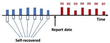
Figure 1: Time train of the progression of infection with COVID-19. Blue or non-filled bars indicate daily new infected cases of type I or II, $D_{1},...,D_{7}$ are the number of reported cases during the 1^th, 2^nd, …, and 7^th day past a given report date (indicated as “Report date”).

In this work, we present a structured approach for an approximate estimation of the number of infected cases at the US national and state level. Statistically, the estimation of the number of unreported cases is related to inference with missing data [13] or censored data [10]. However, certain characteristics of the coronavirus epidemiology allow us to take a different approach. Inspired by the diagnostic analysis of remote sensing studies [21] where the errors in the land use classification were decomposed according to their sources, we distinguish the missing counts in the reported numbers by two sources as illustrated by Figure 1. One source is cases for which, at the time of report, the symptoms were not emerging yet; however, the affected individuals would eventually take a test with results reported. We call such cases the type I cases, and the waiting period before the onset of symptoms is termed as the incubation (or dormant) period. This is illustrated as the filled blue bars in Figure 1. At the time of a given report date (i.e., “Report date” in Figure 1), all such cases are still in dormant status thus are missing in the reported number. A similar figure can be seen in the SIR compartment model considered by [23]. Note the “Report date” in Figure 1 is just a report date that is of interest, and this is true henceforth unless otherwise specified. Usually there is a time gap between the onset of symptoms and the time of report—the infected individual may not immediately take the test and also there might be a delay in reporting (some reported statistics are based on the time of test though). In the lack of relevant data on such delays and for simplicity, we take an integer value slightly larger than the mean incubation periods and use that as the time period to report (i.e., the time period between infection and report, see discussion on the choice of the time window size in Section 2.1).

The second source of unreported cases are those who were infected but are either not aware of it or with symptoms too light to bother, and later on recovered without any particular medical treatments. We call such cases the type II cases. The type II cases are never reflected in any reported numbers, thus leaving too little clue for estimation. But we cannot overlook such cases, since the number of such cases could be potentially large and would form an important source of infection.

We use post-report data for the estimation of the number of type I cases, and population matching to that of type II cases. Due to the intuitive nature and the simplicity in implementation, our approach can be readily applied by the general public or the health department if they wish to obtain an approximate estimate of the actual number of infected cases in order to help understand the situation or to assist policy making and disease control. The remainder of this paper is organized as follows. In Section 2, we will describe our approach. This is followed by a presentation of results in Section 3. Finally we conclude in Section  4.

2 Methods

As stated in Section 1, we take a structured approach by estimating the number of type I and II cases separately. These are described in Section 2.1 and Section 2.2, respectively.

2.1 Estimating the number of type I cases

The estimation of the number of type I cases is facilitated by the following crucial observation. Though not included in the reported number while in the dormant period, such cases would eventually be exposed when the symptoms become so severe that the individuals have to seek medical treatments. By that time, those previously missed cases at the given report date (which was a few days ago) would be counted towards infected cases at some later report dates (though one would not know at which particular report date). Such numbers should be included at the given report date but surface only several days later; for this reason we call them delayed counts. If there is a way to estimate such delayed counts or their total, then one can estimate the number of type I cases for the given report date.

It will be instructive to consider a simple ideal case where all infected cases have an incubation period of 7 days and there is no delay in test taking and reporting. In this ideal case, the numbers $D_{1},D_{2},...,D_{6}$ in Figure 1 are exactly the number of cases who were at their 6^th, 5^th, …, 1^st day of infection (i.e., the time between infection and the given report date), respectively, when counted at the given report date (i.e., “Report date” in Figure 1). As the incubation period for all cases is 7 days, these are all the type I cases missed at the given report date but reflected perfectly later in the number of daily reported cases during the 6 days post-report time window (the window size is 1 day less than the incubation period). So the total number of type I cases at the given report date can be calculated by their sum, $\hat{D}_{type1}=\sum_{i=1}^{6}D_{i}$.

The reality is, however, complicated. First, the incubation period (also the time period to report) varies for individual cases. Also, during the post-report time window, newly infected cases may arise and be reported due to their short incubation periods. Thus the number of daily reported cases at any particular day within this time window might be mixed, in the sense that it would include cases that are infected both before (but were during their incubation period) and after the given report date. The former case will not pose a problem as anyway such cases would be counted towards $\hat{D}_{type1}$ though cases infected on the same day may now contribute to different $D_{i}$’s. The latter case is undesirable but could be corrected, to a certain extent, by the truncating effect when we only sum up the daily counts in the post-report time window up to $T$ days. That is, those cases with a dormant period extending more than $T$ days post-report will be truncated and not included in $\hat{D}_{type1}$, with the total count of such truncated cases being ‘cancelled out’ by the newly infected cases within the time window of length $T$. This leads to an estimate for the number of type I cases as

$$\hat{D}_{type1}=\sum_{1}^{T}D_{i},$$ (1)

where $D_{i}$ are now the number of cases reported at the i^th day after the given report date. By intuition from the ideal case and also accounting for the potential delay in testing and reporting, we can let $T$ take a value around or slightly larger than the mean incubation period.

If we can keep track of the estimate $\hat{D}_{type1}$ through time, then we can get a time series which, upon smoothing, could be used to estimate the current count of type I cases. For such an estimation to be feasible, we have two assumptions. One is that the daily reported counts near the given report date would not change too abruptly. Thus, our approach may not work well when the infection trend rises very rapidly (e.g., during the initial outbreak of the pandemic). During such a period, the safest strategy might be to strictly enforce social distancing. The other is knowledge of the incubation period. A number of studies have been carried out on the estimation of incubation periods, for example, [11, 12] report a median of 4–7 days, [14] gives a mean of 5.8 days, [1] reports a mean of 6.4 days and 6.8 days by fitting the Weibull and lognormal distribution, respectively. While further studies are required, we take $T=7$ in our estimation (which we believe also partially accounts for the time gap between the onset of symptoms and the time of report). Additionally, it should be cautious that our estimation is valid assuming that the test of coronavirus is sufficiently carried out for the population of interest; insufficient test would render an underestimate. Here by sufficient testing we mean whoever or the vast majority of those with symptoms of COVID-19 would take the test. While this was hardly true during the initial outbreak of the pandemic due to resources constraints or public awareness of the pandemic, we believe gradually, at least for the US, it becomes reasonably true.

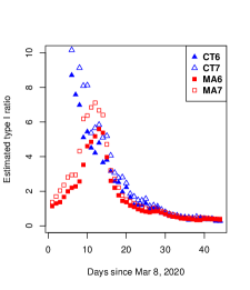
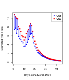
Figure 2: Ratio of unreported cases of Type I w.r.t. reported cases for CT, MA and the US, where ‘6’ and ‘7’ in the legend are the values of $T$ used, respectively.

In Figure 2, we plot the ratio of estimated type I cases w.r.t. the reported number of cases for Connecticut (CT) and Massachusetts (MA) since Mar 8, 2020. These two states were chosen as they are similar in many aspects, such as geography, demography, and population socioeconomics etc which are relevant in the spreading of COVID-19, so we expect their ratio of type I cases out of reported cases would be similar. In Figure 2, there is an initial difference in ratios of type I cases in these two states, which we attribute to the late response and the small number of cases tested in CT, and also possibly some random events such as the well-known Biogen superspreader event in MA in late February. Later, these two states exhibit strikingly similar trend, which is quite expected. We also explore the effect of using different values of $T$ where 6 and 7 are used. Again, initially the resulting estimation are quite different, which indicates the rapid spread of coronavirus and the rapid rise of infected cases. Gradually, the difference in the resulting estimations diminishes, which implies that the choice of $T=7$ leads to a fairly stable estimation after the initial quick growing stage. Similar observation can be made for the estimation of type I cases in US. This is shown in the right panel of Figure 2. In the appendix, we give a statistical justification on why our estimate, $\hat{D}_{type1}$, would be a reasonable one. In particular, we derive an upper bound for the error of this estimate relative to the reported number of infected cases and show that it would be small under mild assumptions about the distribution of the incubation periods and the number of daily new cases.

2.2 Estimating the number of type II cases

The estimation of the number of type II cases is challenging, as there is barely anything observable on the asymptomatic cases. Our main strategy is based on the matching of population statistics—using what we see well to infer what is missing or incomplete. When grouping reported infection cases, we notice a significant discrepancy in the count statistics by different age groups in the US. We expect that, while people in most age groups in the population have a similar chance of being infected, infected individuals of age 65+ are very likely to be discovered timely. This is because people at age 65+ typically have a relatively weaker immune system along with possible pre-existing medical conditions, and a slight symptom would prompt them to seek medical treatments. Indeed the case mortality rate increases exponentially with age, and could be well above 20% for seniors over 70 [20]. Thus reported counts about age groups 65+ would be more accurate and can serve as a reference to correct counts for other age groups. On the contrary, cases for the 20-64 age group are easy to be overlooked or unnoticed, thus their reported counts require a correction (termed as age correction).

Age groups	0-19	20-44	45-54	55-64	65-74	75-84	85+
US population	25.06	33.27	12.73	12.92	9.32	4.70	2.00
Reported cases	5.00	29.00	18.00	18.00	17.00	9.00	6.00
Corrected cases	46.47	61.70	23.61	23.96	17.00	9.00	6.00

Table 1: Percentages by age groups in the US population (2020) and in the reported infection cases. Note numbers in the bottom row are not normalized to sum up to 1.

The age group of 85+ is more vulnerable to infections, as they typically live in the senior centers or extended-care nursing facilities which, as a matter of fact, have a very high risk of infection. The case statistics for this age group would be very thorough, but many in this age group get infected simply because they share a very confined living space with many other equally vulnerable seniors, and the infection of any one in a senior center may quickly spread to the rest (to certain extent, one may think of this as a big indoor party during the pandemic). So statistics in this age group would not be a reliable reference for population match, since people in other age groups have a very different mobility pattern (the infants interact with the world through their parents thus have a chance of infection not so different from the general population).

As a result of equal age susceptibility for people with an age in the range 0-84, the number of infected cases of different age groups would be proportional to their respective percentage in the population. Let $r_{pop}$ and $r_{case}$ be the proportions of the reference group in the population and in the reported cases, and $x_{pop}$ and $x_{corrected}$ be the the respective proportions for the target group, respectively. Then

$$\frac{r_{case}}{r_{pop}}=\frac{x_{corrected}}{x_{pop}},$$

and the corrected percentage in the infected cases for the target group can be calculated accordingly. As we argue before, the case statistics for age groups 65-74 and 75-84 are reliable so they are used as the reference group. A simple calculation reveals that age groups, 65-74 and 75-84, according to Table 1, have a similar ratio of cases percentage: population percentage, i.e., $9.00:4.70\approx 17.00:9.32$. Thus, we can pool counts from these two groups and obtain

$$r_{case}:r_{pop}=(9.00+17.00)/(4.70+9.32)=1.8544.$$

This yields the corrected ratio as the bottom row of Table 1. Adding up numbers in the bottom row gives a total of 187.94%, implying that we should expand the reported counts by 87.94% in order for the reported case counts to match the population statistics across age groups. This gives the ratio of type II cases over the reported cases.

An interesting question is, will estimated counts of type II overlap with that for type I cases? We claim that this will not, at least not significantly, so the addition of estimated counts for type I and II cases is valid. The reason is that, type I cases still contribute to the reported numbers, at a delayed time though. These delayed cases can be thought of as a sample from the reported cases (assuming that the reported cases have a stable proportion when breakdown by age groups). The inclusion of type I cases will not change the age-breakdown proportions. Thus, after the inclusion of type I cases, we still have the same age-breakdown proportions and thus require an age correction.

2.3 Discussions on implications and assumptions

In this section, we will briefly discuss the implications of type I and II ratios and the main assumptions made in our estimation.

The value of type I and II ratios can have important implications to understand the trend of the pandemic or for policy making. If there is no major re-surge of cases, then the type I ratio will slowly decrease with time as a result of the increasing total number of reported cases. Thus as the pandemic continues, type II cases will gradually become the main source of unreported cases. One interesting pattern about the dynamics of type I ratios with time is that a large value or an increase in type I ratio would indicate a quickly growing trend or a re-surge of the pandemic; this can be seen from Figure 2 by the large value of type I ratios in the beginning. It can serve as a strong signal for policy makers or the health department to take immediate actions and for the public to be cautious.

Type II cases are particularly harmful as they are asymptomatic, so it is always highly desirable to reduce the type II ratio. An effective way for this is to increase the coverage of the COVID-19 tests, and to enroll as many individuals as possible (subject to testing capacity) to take the test. Since the summer, many schools or colleges started introducing the asymptomatic test, and we think that has been very effective in helping reduce the type II ratio as these two groups contribute quite substantially to the asymptomatic cases. Also, COVID-19 tests related to travel and the re-opening of many states have helped detect many asymptomatic cases, due to the mandate testing of engaged individuals. Additionally, as more and more individuals are infected, all their close contacts are required to take the test although many are infected but not developing any symptoms. Such cases could be huge due to the exponential social network effect [7]. Studies, including our analysis on more recent data (see appendix), show that the ratio of asymptomatic cases out of all infected ones has reduced from the pre-summer 35-40% to around 20-25% towards the end of the summer.

In estimating the type I ratio, we assume a stable distribution of the daily new infected cases. This may not be realistic during the initial outbreak of the pandemic or later sudden spikes of new cases, and our estimate will potentially overestimate during days around that period. On the other hand, during such period, likely many cases may not be captured by the reported counts. This leads to some cancellation effect to the overestimate, but to what extent is a complicated issue that requires additional information. According to our sensitivity analysis (c.f. Section 3.1), our estimate is fairly robust and incurs a small error when there is a sudden increase of daily new cases by up to 10 times.

One major assumption in estimating the type II ratio is the equal susceptibility across age groups. This is a common assumption made by SIR models for which ages are not explicitly modeled, and we assume this for simplicity. People in age group 0-84 are either exposed to the infection directly, or indirectly through their family members (the chance for household infections is very high), thus it is reasonable to assume that people in this age group have roughly the same chance of infection during the pandemic. Indeed some studies [3] show that the susceptibility is not sensitive to ages. We note that some work in the literature [22, 15] explicitly models the age-specific susceptibility. However, they either use the number of contacts for people in dense cities such as Wuhan and Shanghai in China during a single day as a proxy for age-specific susceptibility [22], or use simulations by locations such as working places, schools or communities etc to estimate age-specific contacts [15]. These studies omit the degrees of contacts and the levels of protections, and explore susceptibility in a single day (which departures from our goal, whether a person may eventually be infected during the pandemic). Moreover, their findings are not applicable to the US as the contact patterns among individuals would be very different, due to huge differences in life and working styles, population density or social distancing policy etc. We believe the difference among different age groups would be small for a sizable population, and the equal susceptibility assumption will facilitate a simple estimation. As many factors potentially contribute to the infection and spread of COVID-19, it is challenging to estimate the age effect but it is a worthwhile problem for further study, and clarifying it may help our estimation and many SIR-based models.

3 Results

We apply our approach to each of the 50 states and the US. The data are available from Wikipedia [19]. Due to the large variation of the population size at different states, we calculate the ratio of missing cases out of the number of reported cases for individual states. The estimated ratios for type I cases for individual states, as of Apr 20, 2020, are shown in Figure 3. The type I ratio for OH, IA, ND and NE are substantially higher than others. This because the infected cases were still quickly rising for OH, IA and ND around the time the type I ratio was calculated. For NE, the accumulated number of reported cases is small so the addition of new daily reported cases may easily lead to a high type I ratio. It should be noted that the ratio of type I cases out of the reported number will decrease as the number of daily reported cases begins stabilizing. This can be seen from Figure 2.

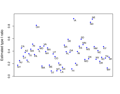
Figure 3: Ratio of type I cases w.r.t. reported cases for each of the 50 states in US on Apr 20, 2020.

Due to the lack of reported case data by age groups for some individual states, we use the overall estimate for the US, which is 87.94% according to discussions in Section 2.2, for the ratio of type II cases for all the states.

The overall ratio of type I cases for the US is estimated to be 32.60% by aggregating estimated type I cases from individual states. Combining with the type II case ratio at 87.94%, this gives an estimated ratio of missing cases versus the reported number at 120.54% for the US. In other words, the reported number of cases for the US should multiply by a factor of 220.54% to reflect the true number of infected cases. This is close to the estimate given in [4] which is twice as large as the number of reported cases for the US as of Apr 17, 2020. Our result implies that the proportion of cases never captured by any medical systems out of all the infected cases is about 87.94/220.54=39.87% as of Apr 20, 2020. This is not far from estimations given by [17] which predicates that the ratio of unidentified cases in NY, NJ, and CA by July 11, 2020 in the range between 18.49% and 33.20%. Our estimate is also consistent to a meta-analysis of over 10 studies [6] which reports an asymptomatic ratio in the range of 15%-40%.

With the unreported numbers estimated, we can estimate the infection ratio, defined as the ratio of the number of infected cases out of the population. The overall infection ratio of the US is estimated to be 0.53%, or 1.75 million infected cases, as of Apr 20, 2020. If we use the associated death toll at about 50k, then the case mortality rate is calculated as 2.85%, which is close to the WHO suggested estimation of 3.4% [18] in March, 2020. The infection ratios for individual states are visualized as heatmap in Figure 4. Heavily hit states are NY, NJ, CT, RI, MA, and LA with infection ratio estimated at 2.61%, 2.11%, 1.22%, 1.15%, 1.31% and 1.04%, respectively, as of Apr 20, 2020. The trend of the infection ratio and cases over time for these states is shown in Figure 5. It can be seen that, except LA, the infection ratios for all other five states are still rapidly increasing. NJ shows a similar growing pattern as NY, while the three New England states, CT, RI and MA, are similar.

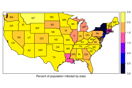
Figure 4: Heatmap of infection ratio for individual states as of Apr 20, 2020.

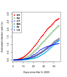
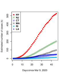
Figure 5: Trend of estimated infection ratio and infected cases for NY, NJ, CT, MA, RI, and LA since Mar 9, 2020.

3.1 Sensitivity analysis

Due to the lack of true infected case counts, we are not able to evaluate the estimation error of our approach empirically. Instead we carry out a sensitivity analysis by simulations, with the goal of evaluating the robustness of our approach under fluctuations of daily new cases. The simulations are conducted as follows. On each day over a span of about 100 days, we generate $N_{i}$ new infected cases with incubation periods following the lognormal or the Weibull distribution. In a given future date, all cases whose incubation period expires will be reported (note cases infected on different dates may be reported on the same day or infected on the same day may be reported on different future dates). On each day, we then compare the actually reported (or unreported) cases to the estimated cases of type I by our algorithm.

The incubation periods are generated according to lognormal [14] or Weibull [1]. We follow the references in their choices of parameters. The lognormal distribution has 1.63 and 0.5 as its mean and standard deviation on the log scale, or 5.80 and 3.08 days for mean and standard deviation of incubation periods. The shape and scale parameters for the Weibull distribution are 3.04 and 7.16, or 6.4 and 2.3 days for the mean and standard deviation, respectively.

To simulate the fluctuation of daily infected cases, we consider four scenarios. One is that the number of daily infected cases is kept at a constant, say, 1000. For the other three cases, we let the number of daily infected cases be sampling from intervals, [600, 1200], [400, 1600], and [200, 2000], respectively, such that the number of new cases can potentially be 2, 4 or 10 times larger, on a certain day, than that of a previous day. Some correlation structures can be imposed on the number of cases during consecutive days, but we opt for simplicity and choose not to pursue it as we aim at simulating different levels of fluctuations of daily new cases. The window size would be 4.8 and 5.4 days for lognormal and Weibull, respectively, in ideal case. But we have to pick an integer value, and also we may need to compensate the potential delays with testing and reporting in practice. So we use window size 5 or 6 for lognormal, and 6 or 7 for Weibull in our simulation. Note that the choice of a large window size may lead to an overestimate of the type I ratio.

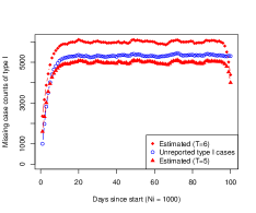
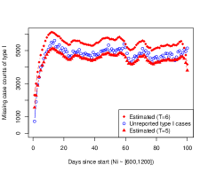
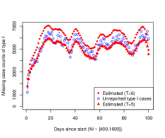
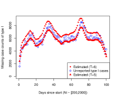
Figure 6: True and estimated number of type I cases with lognormal incubation periods. The window size $T$ used in the estimation are 5 and 6, respectively. The daily infected cases $N_{i}$ are generated under 4 scenarios, constant 1000, uniformly from range [600,1200], [400,1600], and [200,2000], respectively.

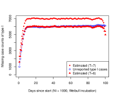
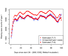
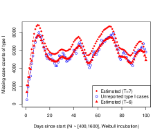
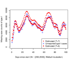
Figure 7: True and estimated number of type I cases and estimated with Weibull incubation periods. The window size $T$ used in the estimation are 6 and 7, respectively. The daily infected cases $N_{i}$ are generated under 4 scenarios, constant 1000, uniformly from range [600,1200], [400,1600], and [200,2000], respectively.

Under all four scenarios, we plot the actually number of unreported cases vs the estimated ones. Figure 6 and Figure 7 are for the lognormal and Weibull distribution, respectively. We also calculate the percentage of errors w.r.t. the number of reported cases and average over 100 days and 100 runs. This is shown in Table 2.

	$N_{i}=1000$	$N_{i}\sim[600,1200]$	$N_{i}\sim[400,1600]$	$N_{i}\sim[200,2000]$
Lognormal (T=5)	1.29%	1.34%	1.60%	1.83%
Lognormal (T=6)	3.11%	3.14%	3.17%	3.22%
Weibull (T=6)	0.38%	0.81%	1.34%	1.75%
Weibull (T=7)	5.02%	5.08%	5.15%	5.27%

Table 2: Mean percentage of errors w.r.t. the number of reported cases over a span of 100 days.

In all cases, the errors are small even when the number of cases fluctuates wildly from time to time. For a smaller window size (i.e., 5 for lognormal and 6 for Weibull), the errors range from 1.29%–1.83% and 0.38%–1.75% for lognormal and Weibull incubation, respectively. For a larger window size (i.e., 6 for lognormal and 7 for Weibull), the errors range from 3.11-3.22% and 5.02–5.27% for lognormal and Weibull, respectively.

4 Conclusions

We have proposed a structured approach for the estimation of the unreported number of infected cases. We distinguish two types of missing cases, those cases which were infected but are still during the dormant period at the time of report and those asymptomatic or light cases which later self-recover without any medical treatments. The number of these two types of cases are estimated by accumulating reported counts within a properly chosen post-report time window and by population matching. The reported number, as of Apr 20, 2020, of infected cases in US should be corrected by multiplying a factor of 220.54%. The overall infection ratio out of the US population is estimated to be 0.53%, implying a case mortality rate of 2.85% as of Apr 20, 2020. The estimate given by our approach also agrees or is close to related estimates by several work in the literature. By Aug 31, 2020, the overall infection ratio in US rises to 2.49% while the case mortality rate decreases to 2.09%, and the ratio of asymptomatic cases out of all infected cases reduces from the pre-summer 35-40% to around 20-25%.

The intuitive nature of our approach makes it easy to understand and to implement, thus we expect it be readily adopted by the general public for understanding the situation or the government for policy making and disease control. Our estimation can potentially be used for risk assessment. The infant age group may worth further consideration as people in this group are much less risky than other age groups as they interact with the rest of the world through their parents, so the number of cases for this group may need to adjust accordingly to reflect the true risk.

Appendix

This appendix consists of two parts. In the first part, we give a justification on our estimation algorithm for the number of type I cases. In the second part, we include analysis on the US COVID-19 data as of August 31, 2020.

A1 Error analysis in the type I estimator

In this section, we show that the error between our estimate, $\hat{D}_{type1}$, of the number of type I cases and its actual value $D_{type1}$ is small in expectation under mild assumptions about the distribution of the incubation periods.

Denote by random variable $X$ the length of the incubation period, and for simplicity we further assume that $X\geq 0$ takes integer values. Let $N_{-1},N_{-2},...$ denote the number of cases that were infected one day, two days and so on before the report date (for which we use $N_{0}$), while $N_{i}$’s indicate those after the report date. Here we limit to type I cases as we can conveniently assume that type II cases have an infinite incubation period. Then the expected number of cases that are discovered during the time window of $T$ days following the given report date is calculated as

$$D_{a}=\sum_{i=0}^{\infty}\mathbb{E}N_{-i}\cdot P(i+1\leq X<i+T).$$ (2)

For simplicity, we would assume that all the $\mathbb{E}N_{-i}$’s take the same value $N$. This is a very mild assumption as we expect that the distribution of the number of newly infected cases per day do not drift much when the pandemic reaches a stable stage (those at the very far distant past would be small, but they carry a very small fraction of the total number so could be ignored). Another simplifying assumption is the independence of $N_{i}$’s and the incubation period $X$. Also, we abuse the notation a bit by using $D_{.}$’s to also indicate the expected value of the associated random variable; the exact meaning will be determined by the context. Then Equation (2) can be rewritten as

$$D_{a} = (T-1)\cdot N-N\sum_{i=1}^{T-1}(T-i)\cdot P(i-1\leq X<i).$$

Under the same assumption, the number of new cases generated during the post-report time window of length $T$ days is

$$D_{new} = \sum_{i=1}^{T}\mathbb{E}N_{i}\cdot P(X<T+1-i)$$

$$= N\sum_{i=1}^{T}(T+1-i)\cdot P(i-1\leq X<i)$$

$$= N\sum_{i=1}^{T-1}(T-i)\cdot P(i-1\leq X<i)+N\cdot P(X<T)$$

Thus the total number of reported cases during the post-report time window of length $T$ days is calculated as

$$D_{a}+D_{new}=(T-1)\cdot N+N\cdot P(X\leq T)=TN-N\cdot P(X>T).$$

Assuming that random variable $X$ has a finite mean, say $\mu$, then we have

$$P(X>T)\leq\mathbb{E}X/T=\mu/T,$$

implying that the estimated number of type I cases satisfies

$$TN\geq\hat{D}_{type1}=D_{a}+D_{new}\geq TN-N\cdot\mu/T.$$ (3)

The actual number of cases that have accumulated but not being discovered before the report date consists of missing cases during the previous $T$ days and those even earlier cases, which has an expected value

$$D_{type1}=\sum_{i=0}^{\infty}\mathbb{E}N_{-i}\cdot P(X\geq i+1)=N\sum_{i=0}^{\infty}P(X\geq i)=N\cdot\mathbb{E}X=\mu N.$$ (4)

(4) indicates that the mean number of type I cases equals the product of the mean daily infected cases of type I and the mean length of the incubation period, which is consistent with the ideal case discussed in Section 2.1. This, along with (3), suggests that the length of the post-report time window should be around the mean of the incubation periods. Let $T=(1+\epsilon)\mu$, then we have the following error bound for the estimated number of cases of type I

$$|\hat{D}_{type1}-D_{type1}|\leq\mu N\cdot\max(\epsilon,|\epsilon-1/T|).$$

It follows that the relative error of the estimate satisfies

$$\frac{|\hat{D}_{type1}-D_{type1}|}{D_{type1}}\leq\max(\epsilon,|\epsilon-1/T|)=\max(\epsilon,|\epsilon-1/((1+\epsilon)\mu)|).$$

For a given $\mu$, one can pick $\epsilon$ to optimize the above bound. For example, when $\mu=7$, one can take $\epsilon=0.07$ to achieve a relative error bound of about 7%.

A2 Analysis on more recent data

We repeat our analysis on data as of August 31, 2020. The data consists in a surge of cases during the summer for many US states, with the reported case count for US increasing by several times from about 830k to 5.94 million since late April. For the new data, our analysis suggests that the number of reported cases for the US be adjusted by a factor of 138.56%, with the ratio of type I and type II cases estimated to be 5.02% and 33.54%, respectively. Both ratios decrease significantly compared to estimates given by data up to Apr 20, 2020. The type I ratio decreases mainly as a result of a major increase in the total number of reported cases, from 830k to 5.94 million. The total number of infected cases in the US is estimated at 8,234,946 as of Aug 31, 2020, implying an overall infection ratio at 2.49%. With a death toll of 171,957, this gives an estimated mortality ratio at 2.09%, which lower than the 2.85% in late Apr, 2020. This is expected, and also observed in many other countries, either because we have now understand more about the virus and hence more informed medical treatments, or likely the virus has gradually become less lethal with time.

Similar as in Section 3, we show the estimated type I ratio for all 50 states as of Aug 31, 2020 (see Figure 8). Compared to Figure 3, the type I ratios of all the states show a significant decrease, which indicates a major slow down of the spread of COVID-19. OH, IA, and NE no longer stand out while ND, along with HI, are still pretty high.

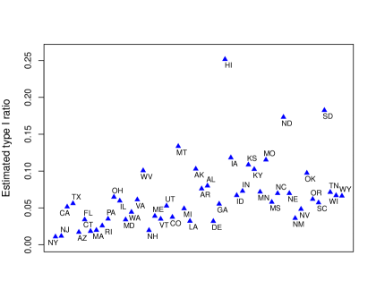
Figure 8: Ratio of type I cases w.r.t. reported cases for each of the 50 states in US as of Aug 31, 2020.

Age groups	0-19	20-44	45-54	55-64	65-74	75-84	85+
US population	25.06	33.27	12.73	12.92	9.32	4.70	2.00
Reported cases	10.84	43.86	15.48	14.40	12.94	5.77	2.76
Corrected cases	33.44	44.40	16.99	17.24	12.94	5.77	2.76

Table 3: Percentages by age groups in the US population (2020) and in the reported infection cases as of August 31, 2020. Note that numbers in the bottom row are not normalized to sum up to 1.

The estimation of type II ratio is based on Table 3. The decrease of type II ratio is likely because a lot more people have now taken the COVID-19 test, not necessarily due to the emerging of symptoms but because, as many states have reopened since the mid of May, people are required to take the test to resume working or to be engaged in summer travels or activities. Also as a lot more individuals are infected, all their close contacts are required to take the test even though many are infected but not showing any symptoms. Such cases could be huge due to the exponential social network effect [7]. The percent of type II cases out of estimated total infected cases is estimated as 33.54%/(1+38.56%)=24.21%. This is comparable to or consistent with a number of recent studies, for example, over 10 studies considered in a meta-analysis [6] report an asymptomatic rate in the range of 15%-40%. With the introduction of asymptomatic tests in a large number of schools, colleges and the general public since the mid of summer, we expect that the type II ratio will further decrease over time and so will the overall ratio of unreported cases.

Similarly, we also calculate the infection ratio and cumulative infected cases for the 6 states NY, NJ, CT, MA, RI and LA up to Aug 31, 2020. The similar trend for all other states pretty much continues except LA, which overtakes the rest and become the highest among all these 6 states; indeed it becomes the highest among all 50 states as well as of Aug 31, 2020, which is likely due to the aggressive re-opening since the mid of May. The top 6 states with highest estimated infection ratios are now LA (4.47%), FL (3.97%), MS (3.89%), AZ (3.83%), AL (3.60%), and GA (3.52%), while the previous (as of Apr 20, 2020) top 6 states have estimated infection ratio as follows: NY (3.14%), NJ (3.02%), CT (2.09%), MA (2.58%), RI (2.92%) and LA (4.47%). Similarly, we also include the heatmap of infection ratios of all 50 US states as of Aug 31, 2020 in Figure 10.

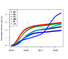
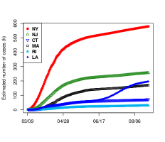
Figure 9: Trend of estimated infection ratio and infected cases for NY, NJ, CT, MA, RI, and LA since Mar 9, 2020.

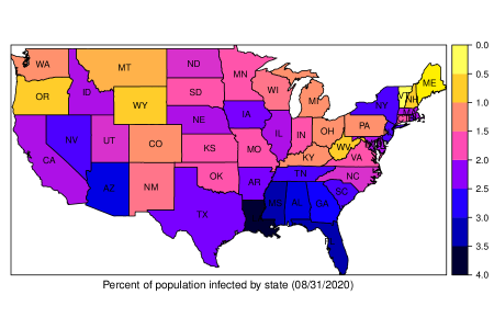
Figure 10: Heatmap of infection ratio for individual states as of Aug 31, 2020.

References

- [1] J. A. Backer, D. Klinkenberg, and J. Wallinga. Incubation period of 2019 novel coronavirus (2019-nCoV) infections among travellers from Wuhan, China, 20–28 January 2020. Eurosurveillance, 25(5), 2020.
- [2] C. Baquero, P. Casari, A. F. Anta, D. Frey, A. Garcia-Agundez, C. Georgiou, R. Menezes, N. Nicolaou, O. Ojo, and P. Patras. Measuring icebergs: Using different methods to estimate the number of COVID-19 cases in Portugal and Spain. medRxiv doi 10.1101/2020.04.20.20073056, 2020.
- [3] Q. Bi, Y. Wu, S. Mei, C. Ye, X. Zou, Z. Zhang, X. Liu, L. Wei, S. Truelove, T. Zhang, W. Gao, C. Cheng, X. Tang, X. Wu, Y. Wu, B. Sun, S. Huang, Y. Sun, J. Zhang, T. Ma, J. Lessler, and T. Feng. Epidemiology and Transmission of COVID-19 in Shenzhen China: Analysis of 391 cases and 1286 of their close contacts. medRxiv doi 10.1101/2020.03.03.20028423, 2020.
- [4] C. Bohk-Ewald, C. Dudel, and M. Myrskyla. A demographic scaling model for estimating the total number of COVID-19 infections. medRxiv doi 10.1101/2020.04.23.20077719, 2020.
- [5] L. Bottcher, M. Xia, and T. Chou. Why estimating population-based case fatality rates during epidemics may be misleading. medRxiv doi 10.1101/2020.03.26.20044693, 2020.
- [6] O. Byambasuren, M. Cardona K. Bell, J. Clark, M. McLaws, and P. Glasziou. Estimating the extent of asymptomatic COVID-19 and its potential for community transmission: Systematic review and meta-analysis. Journal of the Association of Medical Microbiology and Infectious Disease (doi: 10.3138/jammi-2020-0030), 2020.
- [7] D. Easley and J. Kleinberg. Networks, Crowds, and Markets: Reasoning about a Highly Connected World. Cambridge University Press, 2010.
- [8] S. Gupta and R. Shankar. Estimating the number of COVID-19 infections in Indian hot-spots using fatality data. arXiv:2004.04025, 2020.
- [9] K. M. Jagodnik, F. Ray, F. M. Giorgi, and A. Lachmann. Correcting under-reported COVID-19 case numbers: estimating the true scale of the pandemic. medRxiv doi 10.1101/2020.03.14.20036178, 2020.
- [10] E. L. Kaplan and P. Meier. Nonparametric estimation from incomplete observations. Journal of the American Statistical Association, 53(282):457–481, 1958.
- [11] S. A. Lauer, K. Grantz, Q. Bi, F. K. Jones, Q. Zheng, H. Meredith, A. S. Azman, N. G. Reich, and J. Lessler. The incubation period of coronavirus disease 2019 (covid-19) from publicly reported confirmed cases: Estimation and application. Annals of Internal Medicine (doi:10.7326/M20-0504), 2020.
- [12] N. M. Linton, T. Kobayashi, Y. Yang, K. Hayashi, A. R. Akhmetzhanov, S. Jung, B. Yuan, R. Kinoshita, and H. Nishiura. Incubation period and other epidemiological characteristics of 2019 novel coronavirus infections with right truncation: A statistical analysis of publicly available case data. Journal of Clinical Medicine, 9(2):538, 2020.
- [13] R. J. Little and D. Rubin. Statistical Analysis with Missing Data. Wiley, 2002.
- [14] C. McAloon, A. Collins, K. Hunt, A. Barber, A. Byrne, F. Butler, M. Casey, J. Griffin, E. Lane, D. McEvoy, P. Wall, M. Green, L. O’Grady, and S. More. Incubation period of COVID-19: a rapid systematic review and meta-analysis of observational research. British Medical Journal Open, 10(8):1–9, 2020.
- [15] K. Prem, Y. Liu, T. Russell, A. Kucharski, R. Eggo, N. Davies, Centre for the Mathematical Modelling of Infectious Diseases COVID-19 Working Group, M. Jit, and P. Klepac. The effect of control strategies to reduce social mixing on outcomes of the COVID-19 epidemic in Wuhan, China: a modelling study. The Lancet Public Health, 5(5):261–270, 2020.
- [16] P. Richterich. Severe underestimation of COVID-19 case numbers: effect of epidemic growth rate and test restrictions. medRxiv doi 10.1101/2020.04.13.20064220, 2020.
- [17] T. Tian, J. Tan, Y. Jiang, X. Wang, and H. Zhang. Evaluate the timing of resumption of business for the states of New York, New Jersey, and California via a pre-symptomatic and asymptomatic transmission model of COVID-19. medRxiv doi 10.1101/2020.05.16.20103747, 2020.
- [18] WHO. Coronavirus (COVID-19) Mortality Rate, 2020. https://www.worldometers.info/coronavirus/coronavirus-death-rate/.
- [19] Wikipedia. COVID-19 pandemic in the United States, 2020. https://en.wikipedia.org/wiki/COVID-19_pandemic_in_the_United_States.
- [20] D. Yan, A. Chen, and B. Yang. Towards understanding the COVID-19 case fatality rate. arXiv:2103.01313, 2021.
- [21] D. Yan, C. Li, N. Cong, L. Yu, and P. Gong. A structured approach to the analysis of remote sensing images. International Journal of Remote Sensing, 40(20):7874–7897, 2019.
- [22] J. Zhang, M. Litvinova, Y. Liang, Y. Wang, W. Wang, S. Zhao, Q. Wu, S. Merler, C. Viboud, A. Vespignani, M. Ajelli, and H. Yu. Changes in contact patterns shape the dynamics of the covid-19 outbreak in china. Science, 368:1481–1486, 2020.
- [23] T. Zhou and Y. Ji. Semiparametric Bayesian Inference for the Transmission Dynamics of COVID-19 with a State-Space Model. arXiv:2006.05581, 2020.