Skew Gaussian Processes for Classification

Abstract

Gaussian processes (GPs) are distributions over functions, which provide a Bayesian nonparametric approach to regression and classification. In spite of their success, GPs have limited use in some applications, for example, in some cases a symmetric distribution with respect to its mean is an unreasonable model. This implies, for instance, that the mean and the median coincide, while the mean and median in an asymmetric (skewed) distribution can be different numbers. In this paper, we propose Skew-Gaussian processes (SkewGPs) as a non-parametric prior over functions. A SkewGP extends the multivariate Unified Skew-Normal distribution over finite dimensional vectors to a stochastic processes. The SkewGP class of distributions includes GPs and, therefore, SkewGPs inherit all good properties of GPs and increase their flexibility by allowing asymmetry in the probabilistic model. By exploiting the fact that SkewGP and probit likelihood are conjugate model, we derive closed form expressions for the marginal likelihood and predictive distribution of this new nonparametric classifier. We verify empirically that the proposed SkewGP classifier provides a better performance than a GP classifier based on either Laplace’s method or Expectation Propagation.

1 Introduction

Gaussian processes (GPs) extend multivariate Gaussian distributions over finite dimensional vectors to infinite dimensionality. Specifically, a GP defines a distribution over functions, that is each draw from a Gaussian process is a function. Therefore, GPs provide a principled, practical, and probabilistic approach to nonparametric regression and classification and they have successfully been applied to different domains (Rasmussen and Williams, 2006).

GPs have several desirable mathematical properties. The most appealing of them is that, for regression with Gaussian noise, the prior distribution is conjugate for the likelihood function. Therefore the Bayesian update step is analytic, as is computing the predictive distribution for the function behavior at unknown locations. In spite of their success, GPs have several known shortcomings.

First, the Gaussian distribution is not a “heavy-tailed” distribution, and so it is not robust to extreme outliers. Alternative to GPs have been proposed of which the most notable example is represented by the class of elliptical processes (Fang, 2018), such as Student-t processes (O’Hagan, 1991; Zhang et al., 2007), where any collection of function values has a desired elliptical distribution, with a covariance matrix built using a kernel.

Second, the Gaussian distribution is symmetric with respect to its mean. This implies, for instance, that the mean and the median coincide, while the mean and median in an asymmetric (skewed) distribution can be different numbers. This constraint limits GPs’ flexibility and affects the coverage of their credible intervals (regions) – especially when considering that symmetry must hold for all components of the (latent) function and that, as for instance discussed by Kuss and Rasmussen (2005); Nickisch and Rasmussen (2008), the exact posterior of a GP classifier is skewed.

To overcome this second limitation, in this paper, we propose Skew-Gaussian processes (SkewGPs) as a non-parametric prior over functions. A SkewGP extends the multivariate Unified Skew-Normal distribution defined over finite dimensional vectors to a stochastic process, i.e. a distribution over infinite dimensional objects. A SkewGP is completely defined by a location function, a scale function and three additional parameters that depend on a latent dimension: a skewness function, a truncation vector and a covariance matrix. It is worth noting that a SkewGP reduces to a GP when the latent variables have dimension zero. Therefore, SkewGPs inherit all good properties of GPs and increase their flexibility by allowing asymmetry in the probabilistic model.

We focus on applying this new nonparametric model to a classification problem. In the case of parametric models, Durante (2018) shows that the posterior distribution of a probit likelihood and Gaussian prior has a unified skew-normal distribution. Such a novel result allowed the author to efficiently compute full posterior inferences for Bayesian logistic regression (for small datasets $n\approx 100$). Moreover the author showed that the unified skew-normal distribution is a conjugate prior for the probit likelihood (without using this prior model for data analysis).

Here we extend this result to the nonparametric case, we derive a semi-analytical expression for the posterior distribution of the latent function and predictive probabilities for SkewGPs. The term semi-analytical is adopted to indicate that posterior inferences require the computation of the cumulative distribution function of a multivariate Gaussian distribution (i.e., the computation of Gaussian orthant probabilities). By using a new formulation (Gessner et al., 2019) of elliptical slice sampling (Murray et al., 2010), lin-ess, which permits efficient sampling from a linearly constrained (e.g., orthant) Gaussian domain, we show that we can compute efficiently posterior inferences for SkewGP binary classifiers. Lin-ess is a special case of elliptical slice sampling that leverages the analytic tractability of intersections of ellipses and hyperplanes to speed up the elliptical slice algorithm. In particular, this guarantees rejection-free sampling and it is therefore also highly parallelizable.

The main contributions of this paper are

1. we propose a new class of stochastic processes called Skew-Gaussian processes (SkewGP) which generalize GP models;

2. we show that a SkewGP prior process is conjugate for the probit likelihood thus deriving for the first time the posterior distribution of a GP classifier in an analytic form;

3. we derive an efficient way to learn the hyperparameters of SkewGP and compute Monte Carlo predictions using lin-ess, showing that our model has similar bottleneck computational complexity of GPs;

4. we evaluate the proposed SkewGP classifier against state-of-the-art implementations of the GP classifier which approximate the posterior with the Laplace method or with Expectation propagation;

5. we show on a small image classification dataset that a SkewGP prior can lead to better uncertainty quantification than a GP prior.

2 Background

The skew normal distribution is a continuous probability distribution that generalises the normal distribution to allow for non-zero skewness. The probability density function (PDF) of the univariate skew-normal distribution with location $\xi\in\mathbb{R}$, scale $\sigma>0$ and skew parameter $\alpha\in\mathbb{R}$ is given by (O’Hagan and Leonard, 1976):

$$p(z)={\frac{2}{\sigma}}\phi\left({\frac{z-\xi}{\sigma}}\right)\Phi\left(\alpha\left({\frac{z-\xi}{\sigma}}\right)\right),\qquad z\in\mathbb{R}$$

where $\phi$ and $\Phi$ are the PDF and, respectively, Cumulative Distribution Function (CDF) of the standard univariate Normal distribution. This distribution has been generalised in several ways, see (Azzalini, 2013) for a review. In particular, Arellano and Azzalini (2006) provided a unification of the above generalizations within a single and tractable multivariate Unified Skew-Normal distribution that satisfies closure properties for marginals and conditionals and allows more flexibility due the introduction of additional parameters.

2.1 Unified Skew-Normal distribution

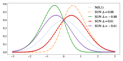
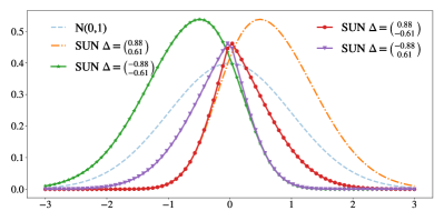
(a1) $s=1$, $\Gamma=1$	(a2) $s=2$, $\Gamma_{1,2}=0.88$

Figure 1: Density plots for $\text{SUN}_{1,s}(0,1,\Delta,\gamma,\Gamma)$. For all plots $\Gamma$ is a correlation matrix, $\gamma=0$, dashed lines are the contour plots of $y\sim N_{1}(0,1)$.

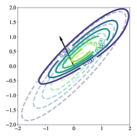
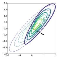
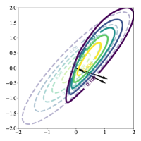
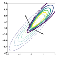
(a1) $s=1$, $\Gamma=1$	(a2) $s=1$, $\Gamma=1$	(a3) $s=2$, $\Gamma_{1,2}=0.96$	(a4) $s=2$, $\Gamma_{1,2}=0.33$
$\Delta=[0.88,0.61]^{T}$,	$\Delta=[0.61,0.88]^{T}$	$\Delta=\begin{bmatrix}0.61&0.76\\ 0.88&,0.97\end{bmatrix}$	$\Delta=\begin{bmatrix}0.61&0.88\\ 0.88&0.61\end{bmatrix}$

Figure 2: Contour density plots for four unified skew-normal. For all plots $p=2$, $\boldsymbol{[}\xi]=[0,0]^{T}$, $\Omega$ and $\Gamma$ are correlation matrices with $\Omega_{1,2}=0.88$, $\gamma=0$, dashed lines are the contour plots of $y\sim N_{2}(\boldsymbol{[}\xi],\Omega)$.

A vector $\boldsymbol{[}z]\in\mathbb{R}^{p}$ is said to have a multivariate Unified Skew-Normal distribution with latent skewness dimension $s$, $\boldsymbol{[}z]\sim\text{SUN}_{p,s}(\boldsymbol{[}\xi],\Omega,\Delta,\boldsymbol{[}\gamma],\Gamma)$, if its probability density function (Azzalini, 2013, Ch.7) is:

$$p(\boldsymbol{[}z])=\phi_{p}(\boldsymbol{[}z]-\boldsymbol{[}\xi];\Omega)\frac{\Phi_{s}\left(\boldsymbol{[}\gamma]+\Delta^{T}\bar{\Omega}^{-1}D_{\Omega}^{-1}(\boldsymbol{[}z]-\boldsymbol{[}\xi]);\Gamma-\Delta^{T}\bar{\Omega}^{-1}\Delta\right)}{\Phi_{s}\left(\boldsymbol{[}\gamma];\Gamma\right)}$$ (1)

where $\phi_{p}(\boldsymbol{[}z]-\boldsymbol{[}\xi];\Omega)$ represents the PDF of a multivariate Normal distribution with mean $\boldsymbol{[}\xi]\in\mathbb{R}^{p}$ and covariance $\Omega=D_{\Omega}\bar{\Omega}D_{\Omega}\in\mathbb{R}^{p\times p}$, with $\bar{\Omega}$ being a correlation matrix and $D_{\Omega}$ a diagonal matrix containing the square root of the diagonal elements in $\Omega$. The notation $\Phi_{s}(\boldsymbol{[}a];M)$ denotes the CDF of $N_{s}(0,M)$ evaluated at $\boldsymbol{[}a]\in\mathbb{R}^{s}$. The parameters $\boldsymbol{[}\gamma]\in\mathbb{R}^{s},\Gamma\in\mathbb{R}^{s\times s},\Delta^{p\times s}$ of the SUN distribution are related to a latent variable that controls the skewness, in particular $\Delta$ is called Skewness matrix. The PDF (1) is well-defined provided that the matrix

$$M:=\begin{bmatrix}\Gamma&\Delta^{T}\\ \Delta&\bar{\Omega}\end{bmatrix}\in\mathbb{R}^{(s+p)\times(s+p)}>0,$$ (2)

i.e., $M$ is positive definite. Note that when $\Delta=0$, (1) reduces to $\phi_{p}(\boldsymbol{[}z]-\boldsymbol{[}\xi];\Omega)$. Moreover we assume that $\Phi_{0}(\cdot)=1$, so that, for $s=0$, (1) becomes a multivariate Normal distribution.

The role of the latent dimension $s$ can be briefly explained as follows. Consider now a random vector $\begin{bmatrix}\boldsymbol{[}x]_{0}\\ \boldsymbol{[}x]_{1}\end{bmatrix}\sim N_{s+p}(0,M)$ with $M$ as in (2) and define $\mathbf{y}$ as the vector with distribution $(\boldsymbol{[}x]_{1}\mid\boldsymbol{[}x]_{0}+\boldsymbol{[}\gamma]>0)$, then it can be shown (Azzalini, 2013, Ch. 7) that $\boldsymbol{[}z]=\boldsymbol{[}\xi]+D_{\Omega}\mathbf{y}\sim\text{SUN}_{p,s}(\boldsymbol{[}\xi],\Omega,\Delta,\boldsymbol{[}\gamma],\Gamma)$. This representation will be used in Section 5 to draw samples from the distribution. Figure 1 shows the density of a univariate SUN distribution with latent dimensions $s=1$ (a1) and $s=2$ (a2). The effect of a higher latent dimension can be better observed in bivariate SUN densities as shown in Figure 2. The contours of the corresponding bivariate normal are dashed. We also plot the skewness directions given by $\bar{\Omega}^{-1}\Delta$.

The Skew-Normal family has several interesting properties, see Azzalini (2013, Ch.7) for details. Most notably, it is close under marginalization and affine transformations. Specifically, if we partition $z=[z_{1},z_{2}]^{T}$, where $z_{1}\in\mathbb{R}^{p_{1}}$ and $z_{2}\in\mathbb{R}^{p_{2}}$ with $p_{1}+p_{2}=p$, then

$$\begin{array}[]{c}z_{1}\sim SUN_{p_{1},s}(\boldsymbol{[}\xi]_{1},\Omega_{11},\Delta_{1},\boldsymbol{[}\gamma],\Gamma),\vspace{0.2cm}\\ \text{with }~{}~{}\boldsymbol{[}\xi]=\begin{bmatrix}\boldsymbol{[}\xi]_{1}\\ \boldsymbol{[}\xi]_{2}\end{bmatrix},~{}~{}~{}\Delta=\begin{bmatrix}\Delta_{1}\\ \Delta_{2}\end{bmatrix},~{}~{}~{}\Omega=\begin{bmatrix}\Omega_{11}&\Omega_{12}\\ \Omega_{21}&\Omega_{22}\end{bmatrix}.\end{array}$$ (3)

Moreover, (Azzalini, 2013, Ch.7) the conditional distribution is a unified skew-Normal, i.e., $(Z_{2}|Z_{1}=z_{1})\sim SUN_{p_{2},s}(\boldsymbol{[}\xi]_{2|1},\Omega_{2|1},\Delta_{2|1},\boldsymbol{[}\gamma]_{2|1},\Gamma_{2|1})$, where

$$\boldsymbol{[}\xi]_{2|1} :=\boldsymbol{[}\xi]_{2}+\Omega_{21}\Omega_{11}^{-1}(z_{1}-\boldsymbol{[}\xi]_{1}),\quad\Omega_{2|1}:=\Omega_{22}-\Omega_{21}\Omega_{11}^{-1}\Omega_{12},$$

$$\Delta_{2|1} :=\Delta_{2}-\bar{\Omega}_{21}\bar{\Omega}_{11}^{-1}\Delta_{1},$$

$$\boldsymbol{[}\gamma]_{2|1} :=\boldsymbol{[}\gamma]+\Delta_{1}^{T}\Omega_{11}^{-1}(z_{1}-\boldsymbol{[}\xi]_{1}),\quad\Gamma_{2|1}:=\Gamma-\Delta_{1}^{T}\bar{\Omega}_{11}^{-1}\Delta_{1},$$

and $\bar{\Omega}_{11}^{-1}:=(\bar{\Omega}_{11})^{-1}$.

3 Skew-Gaussian process

In this section, we define a Skew-Gaussian Process (SkewGP). Consider the functions $\xi:\mathbb{R}^{p}\rightarrow\mathbb{R}$, a location function, $\Omega:\mathbb{R}^{p}\times\mathbb{R}^{p}\rightarrow\mathbb{R}$, a scale function, $\Delta:\mathbb{R}^{p}\rightarrow\mathbb{R}^{s}$, the Skewness vector function, and $\boldsymbol{[}\gamma]\in\mathbb{R}^{s},\Gamma\in\mathbb{R}^{s\times s}$.

We say that a real function $f:\mathbb{R}^{p}\rightarrow\mathbb{R}$ is distributed as a skew-Gaussian process with latent dimension $s$, if, for any sequence of $n$ points $\boldsymbol{[}x]_{1},\dots,\boldsymbol{[}x]_{n}\in\mathbb{R}^{p}$, the vector $f(X)=[f(\boldsymbol{[}x]_{1}),\dots,f(\boldsymbol{[}x]_{n})]^{T}$ is Skew-Gaussian distributed with parameters $\boldsymbol{[}\gamma],\Gamma$, location, scale and skewness matrices, respectively, given by

$$\begin{array}[]{rl}\xi(X):=\begin{bmatrix}\xi(\boldsymbol{[}x]_{1})\\ \xi(\boldsymbol{[}x]_{2})\\ \vdots\\ \xi(\boldsymbol{[}x]_{n})\\ \end{bmatrix},~{}~{}\Omega(X,X)&:=\begin{bmatrix}\Omega(\boldsymbol{[}x]_{1},\boldsymbol{[}x]_{1})&\Omega(\boldsymbol{[}x]_{1},\boldsymbol{[}x]_{2})&\dots&\Omega(\boldsymbol{[}x]_{1},\boldsymbol{[}x]_{n})\\ \Omega(\boldsymbol{[}x]_{2},\boldsymbol{[}x]_{1})&\Omega(\boldsymbol{[}x]_{2},\boldsymbol{[}x]_{2})&\dots&\Omega(\boldsymbol{[}x]_{2},\boldsymbol{[}x]_{n})\\ \vdots&\vdots&\dots&\vdots\\ \Omega(\boldsymbol{[}x]_{n},\boldsymbol{[}x]_{1})&\Omega(\boldsymbol{[}x]_{n},\boldsymbol{[}x]_{2})&\dots&\Omega(\boldsymbol{[}x]_{n},\boldsymbol{[}x]_{n})\\ \end{bmatrix},\vspace{0.2cm}\\ \Delta(X)&:=\begin{bmatrix}~{}~{}\Delta(\boldsymbol{[}x]_{1})&\quad\quad\Delta(\boldsymbol{[}x]_{2})&~{}~{}\dots&~{}\quad\Delta(\boldsymbol{[}x]_{n})\\ \end{bmatrix}.\end{array}$$ (4)

The Skew-Gaussian distribution above is well defined provided that the matrix

$$\begin{bmatrix}\Gamma&\Delta(X)\\ \Delta(X)^{T}&\Omega(X,X)\end{bmatrix}$$

is positive definite for all $X=\{\boldsymbol{[}x]_{1},\dots,\boldsymbol{[}x]_{n}\}\subset\mathbb{R}^{p}$ and for all $n$. In this case we can write

$$f(\boldsymbol{[}x])\sim\text{SkewGP}_{s}(\xi(\boldsymbol{[}x]),\Omega(\boldsymbol{[}x],\boldsymbol{[}x]^{\prime}),\Delta(\boldsymbol{[}x],\boldsymbol{[}x]^{\prime}),\boldsymbol{[}\gamma],\Gamma).$$ (5)

We detail how to select the parameters in Section 4, the proposition below shows that SkewGP is a proper stochastic process.

Proposition 1

The construction of a Skew-Gaussian process from a finite-dimensional distribution is well-posed.

All the proofs are in appendix.

3.1 Binary classification

Consider the training data $\mathcal{D}=\{(\boldsymbol{[}x]_{i},y_{i})\}_{i=1}^{n}$, where $\boldsymbol{[}x]_{i}\in\mathbb{R}^{p}$ and $y_{i}\in\{0,1\}$. We aim to build a nonparametric binary classifier. We first define a probabilistic model $\mathcal{M}$ by assuming that $f\sim\text{SkewGP}(\xi,\Omega,\Delta,\boldsymbol{[}\gamma],\Gamma)$ and considering a probit model for the likelihood:

$$p(\mathcal{D}|f) =\prod\limits_{i=1}^{n}\Phi(f(\boldsymbol{[}x]_{i});1)^{y_{i}}(1-\Phi(f(\boldsymbol{[}x]_{i});1))^{1-y_{i}}=\prod\limits_{i=1}^{n}\Phi((2y_{i}-1)f(\boldsymbol{[}x]_{i});1)$$ (6)

$$=\Phi_{n}(Wf(X);I_{n}),$$

where $W=\text{diag}(2y_{1}-1,\dots,2y_{n}-1)$. A SkewGP prior combined with a probit likelihood gives rise to a posterior SkewGP over functions, this because Skew-Gaussian distributions are conjugate priors for probit models. In the finite dimensional parametric case, this property was shown by Durante (2018), hereafter we extend it to the nonparametric one.

Theorem 3.1

The posterior of $f(X)$ is a Skew-Gaussian distribution:

$$p(f(X)|\mathcal{D}) =\text{SUN}_{n,s+n}(\tilde{\xi},\tilde{\Omega},\tilde{\Delta},\tilde{\boldsymbol{[}\gamma]},\tilde{\Gamma})$$ (7)

$$\tilde{\xi} =\xi,\qquad\tilde{\Omega}=\Omega,$$ (8)

$$\tilde{\Delta} =[\Delta,~{}~{}\bar{\Omega}D_{\Omega}W^{T}],$$ (9)

$$\tilde{\boldsymbol{[}\gamma]} =[\boldsymbol{[}\gamma],~{}~{}W\xi]^{T},$$ (10)

$$\tilde{\Gamma} =\begin{bmatrix}\Gamma&~{}~{}\Delta^{T}D_{\Omega}W^{T}\\ WD_{\Omega}\Delta&~{}~{}(W\Omega W^{T}+I_{n})\end{bmatrix},$$ (11)

where, for simplicity of notation, we have denoted $\xi(X),\Omega(X,X),\Delta(X)$ as $\xi,\Omega,\Delta$ and $\Omega=D_{\Omega}\bar{\Omega}D_{\Omega}$.

From Theorem 3.1 we can immediately derive the following result.

Corollary 1

The marginal likelihood of the observations $\mathcal{D}=\{(\boldsymbol{[}x]_{i},y_{i})\}_{i=1}^{n}$ given the probabilistic model $\mathcal{M}$, that is the prior (5) and likelihood (6), is

$$p(\mathcal{D}|\mathcal{M})=\frac{\Phi_{s+n}(\tilde{\boldsymbol{[}\gamma]};~{}\tilde{\Gamma})}{\Phi_{s}(\boldsymbol{[}\gamma];~{}\Gamma)},$$ (12)

with $\tilde{\boldsymbol{[}\gamma]},\tilde{\Gamma}$ defined in Theorem 3.1.

In classification, based on the training data $\mathcal{D}=\{(\boldsymbol{[}x]_{i},y_{i})\}_{i=1}^{n}$, and given test inputs $\boldsymbol{[}x]^{*}$, we aim to predict the probability that $y^{*}=1$.

Corollary 2

The posterior predictive probability of $y^{*}=1$ given the test input $\boldsymbol{[}x]^{*}\in\mathbb{R}^{p}$ and the training data $\mathcal{D}=\{(\boldsymbol{[}x]_{i},y_{i})\}_{i=1}^{n}$ is

$$p(y^{*}=1|\boldsymbol{[}x]^{*},X,y)=\frac{\Phi_{s+n+1}(\tilde{\boldsymbol{[}\gamma]}^{*};~{}\tilde{\Gamma}^{*})}{\Phi_{s+n}(\tilde{\boldsymbol{[}\gamma]};~{}\tilde{\Gamma})},$$ (13)

where $\tilde{\boldsymbol{[}\gamma]}^{*},\tilde{\Gamma}^{*}$ are the corresponding matrices of the posterior computed for the augmented dataset $\hat{X}=[X^{T},{\boldsymbol{[}x]^{*}}^{T}]^{T}$, $\hat{y}=[y^{T},1/2]^{T}$.

Note that the dummy value $\frac{1}{2}$ in $\hat{y}$ does not influence the value of $p(y^{*}=1|\boldsymbol{[}x]^{*},X,y)$ and it was chosen only for mathematical convenience, as it allows for marginalization over $f(\boldsymbol{[}x]^{*})$ and to derive the expression of $\tilde{\boldsymbol{[}\gamma]}^{*},\tilde{\Gamma}^{*}$ similarly to the ones in Theorem 3.1.

4 Prior functions, parameters and hyperparameters

A SkewGP prior is completely defined by the location function $\xi(\boldsymbol{[}x])$, the scale function $\Omega(\boldsymbol{[}x],\boldsymbol{[}x]^{\prime})$, the latent dimension $s\in\mathbb{N}$, the skewness vector function $\Delta(\boldsymbol{[}x],\boldsymbol{[}x]^{\prime})\in\mathbb{R}^{s}$ and $\boldsymbol{[}\gamma]\in\mathbb{R}^{s},\Gamma\in\mathbb{R}^{s\times s}$. As it is common for GPs, we will take the location function $\xi(\boldsymbol{[}x])$ to be zero, although this need not be done. Let $K(\boldsymbol{[}x],\boldsymbol{[}x]^{\prime})$ be a positive definite covariance function (kernel) and let $\Omega=K(X,X)$ be the covariance matrix obtained by applying $K(\boldsymbol{[}x],\boldsymbol{[}x]^{\prime})$ elementwise to the training data $X$. In this paper, we propose the following way to define the location, scale and skewness functions of a SkewGP:

$$M=\begin{bmatrix}\Gamma&\Delta(X,R)^{T}\\ \Delta(X,R)&\bar{\Omega}(X,X)\end{bmatrix}:=\begin{bmatrix}L\bar{K}(R,R)L&~{}~{}L\bar{K}(R,X)\\ \bar{K}(X,R)L&~{}~{}\bar{K}(X,X)\end{bmatrix},$$ (14)

with $L\in\mathbb{R}^{s\times s}$ is a diagonal matrix whose elements $L_{ii}\in\{-1,1\}$ (it is a phase), $R=[\boldsymbol{[}r]_{1},\dots,\boldsymbol{[}r]_{s}]^{T}\in\mathbb{R}^{s\times p}$ is a vector of $s$ pseudo-points and $\bar{K}(\boldsymbol{[}x],\boldsymbol{[}x]^{\prime})=\frac{1}{\sigma^{2}}K(\boldsymbol{[}x],\boldsymbol{[}x]^{\prime})$ (for stationary kernels) with $K(\boldsymbol{[}x],\boldsymbol{[}x]^{\prime})$ being the kernel function and $\sigma^{2}$ the variance parameter of the kernel, e.g., for the RBF kernel

$$K(\boldsymbol{[}x],\boldsymbol{[}x]^{\prime}):=\sigma^{2}\exp\left(-\frac{\|{\boldsymbol{[}x]}-{\boldsymbol{[}x]^{\prime}}\|^{2}}{2\ell^{2}}\right).$$

It can easily be proven that $M>0$ and, therefore, (2) holds. We select the parameters of the kernel $\sigma,\ell$, the locations $\boldsymbol{[}r]_{i}$ of the pseudo-points and the phase diagonal matrix $L$ by maximizing the marginal likelihood. In particular we exploit the lower bound (16) explained in Section 5.

Similarly to the inducing points in the sparse approximation of GPs (Quiñonero-Candela and Rasmussen, 2005; Snelson and Ghahramani, 2006; Titsias, 2009; Bauer et al., 2016), the points $\boldsymbol{[}r]_{i}$ can be viewed as a set of $s$ latent variables. However, their role is totally different from that of the inducing points, they allow us to locally modulate the skewness of SkewGP. Figure 3 shows latent functions (in gray, second column) drawn from a SkewGP with latent dimension $2$ and the result of squashing these sample functions through the probit logistic function (first column). In all cases, we have considered $\xi(\boldsymbol{[}x])=0$ and a RBF kernel with $\ell=0.3$ and $\sigma^{2}=1$. The values of the other parameters of the SkewGP are reported at the top of the plots in the first column. The green line is the mean function and the red dots represent the location of the $s=2$ latent pseudo-points. For large positive values of $\gamma_{1},\gamma_{2}$, SkewGP is equivalent to a GP (plots (a1)-(a2)). At the decreasing of $\gamma_{i}$, $i=1,2$ (plots (b1)-(b2)), the mean shifts up and the mass of the distribution is concentrated on the top of the figure. By changing the phase (the sign of) $L_{22}$ (plots (c1)-(c2)), the mean and the mass of the distribution shift down at the location of the second pseudo-observation $r_{2}$. We can magnifying this effect by decreasing both $\gamma_{i}$ (plots (d1)-(d2)). It is also possible to introduce skewness without changing the mean (plots (e1)-(e2)). In this latter case, $r_{1}=r_{2}$ and the mass of the distribution is shifted up.

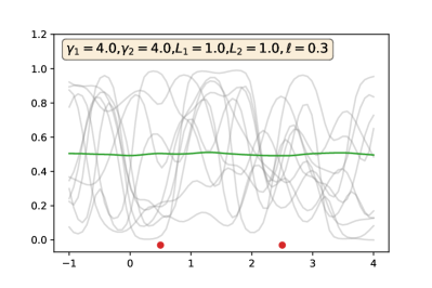
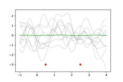
(a1)	(a2)
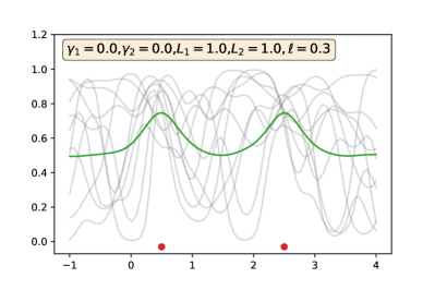
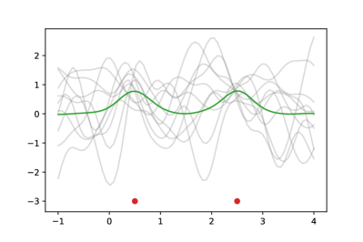
(b1)	(b2)
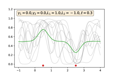
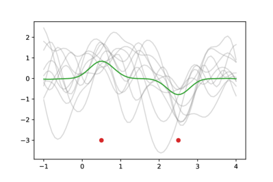
(c1)	(c2)
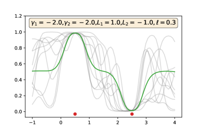
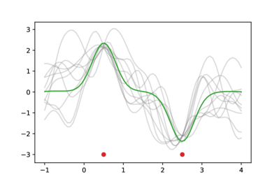
(d1)	(d2)
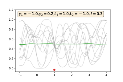
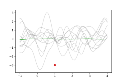
(e1)	(e2)

Figure 3: The second column shows random latent functions (in gray) drawn from a SkewGP with latent dimension $2$ and the first column shows the result of squashing these sample functions through the probit logistic function. The values of the parameters of the SkewGP are reported at the top of the plots in the first column. The green line is the mean function and the red dots represent the location of the $s=2$ latent pseudo-points.

5 Computational complexity

Corollaries 1 and 2 provide two straightforward ways to compute the marginal likelihood and the predictive posterior probability however equations (12) and (13) both require the accurate computation of $\Phi_{s+n}$. Quasi-randomized Monte Carlo methods (Genz, 1992; Genz and Bretz, 2009; Botev, 2017) allows calculation of $\Phi_{s+n}$ for small $n$ (few hundreds observations). Therefore, these procedures are not in general suitable for medium and large $n$ (apart from special cases Phinikettos and Gandy (2011); Genton et al. (2018); Azzimonti and Ginsbourger (2018)). We overcome this issue with an effective use of sampling for the predictive posterior and a mini-batch approach to marginal likelihood.

Posterior predictive distribution.

In order to compute the predictive distribution we generate samples from the posterior distribution at training points and then exploit the closure properties of the SUN distribution to obtain samples at test points. The following result from Azzalini (2013) allows us to draw independent samples from the posterior in (7):

$$f(X) \sim\tilde{\xi}+D_{\Omega}\left(U_{0}+\tilde{\Delta}\tilde{\Gamma}^{-1}U_{1}\right),$$ (15)

$$U_{0} \sim\mathcal{N}(0;\bar{\Omega}-\tilde{\Delta}\tilde{\Gamma}^{-1}\tilde{\Delta}^{T}),\qquad U_{1}\sim\mathcal{T}_{\tilde{\boldsymbol{[}\gamma]}}(0;\tilde{\Gamma}),$$

where $\mathcal{T}_{\tilde{\boldsymbol{[}\gamma]}}(0;\tilde{\Gamma})$ is the pdf of a multivariate Gaussian distribution truncated component-wise below $-\tilde{\boldsymbol{[}\gamma]}$. Equation (15) is a consequence of the additive representation of skew-normal distributions, see (Azzalini, 2013, Ch. 7.1.2 and 5.1.3) for more details. Note that sampling $U_{0}$ can be achieved with standard methods, however using standard rejection sampling for the variable $U_{1}$ would incur in exponentially growing sampling time as the dimension increases. A commonly used sampling technique for this type of problems is Elliptical Slice Sampling (ess) (Murray et al., 2010) which is a Markov Chain Monte Carlo algorithm that performs inference in models with Gaussian priors. This method looks for acceptable samples along elliptical slices and by doing so drastically reduces the number of rejected samples. Recently, Gessner et al. (2019) proposed an extension of ess, called linear elliptical slice sampling (lin-ess), for multivariate Gaussian distribution truncated on a region defined by linear constraints. In particular, this approach analytically derives the acceptable regions on the elliptical slices used in ess and thus guarantees rejection-free sampling. This leads to a large speed up over ess, especially in high dimensions.

Given posterior samples at the training points it is possible to compute the predictive posterior at a new test points $\boldsymbol{[}x]^{*}$ thanks to the following result.

Theorem 5.1

The posterior samples of the latent function computed at the test point $\boldsymbol{[}x]^{*}$ can be obtained by sampling $f(\boldsymbol{[}x]^{*})$ from:

$$f(\boldsymbol{[}x]^{*}) \sim SUN_{1,s}({\xi}_{*},{\Omega}_{*},{\Delta}_{*},{\boldsymbol{[}\gamma]}_{*},{\Gamma}_{*}),$$

$${\xi}_{*} =\xi(\boldsymbol{[}x]^{*})+K(\boldsymbol{[}x]^{*},X)K(X,X)^{-1}(f(X)-\xi(X)),$$

$${\Omega}_{*} =K(\boldsymbol{[}x]^{*},\boldsymbol{[}x]^{*})-K(\boldsymbol{[}x]^{*},X)K(X,X)^{-1}K(X,\boldsymbol{[}x]^{*}),$$

$${\Delta_{*}} =\Delta(\boldsymbol{[}x]^{*})-\bar{K}(\boldsymbol{[}x]^{*},X)\bar{K}(X,X)^{-1}\Delta(X),$$

$${\boldsymbol{[}\gamma]_{*}} =\boldsymbol{[}\gamma]+\Delta(X)^{T}\bar{K}(X,X)^{-1}D_{\Omega}(X,X)^{-1}(f(X)-\xi(X)),$$

$${\Gamma_{*}} =\Gamma-\Delta(X)^{T}\bar{K}^{-1}\Delta(X),$$

with $f(X)$ sampled from the posterior $\text{SUN}_{n,s+n}(\tilde{\xi},\tilde{\Omega},\tilde{\Delta},\tilde{\boldsymbol{[}\gamma]},\tilde{\Gamma})$ in Theorem 3.1, $K$ is a kernel that defines the matrices $\Gamma,\Delta,\Omega$ as in eq. (14) and where

$$\begin{bmatrix}\bar{K}(X,X)&\bar{K}(X,\boldsymbol{[}x]^{*})\\ \bar{K}(\boldsymbol{[}x]^{*},X)&\bar{K}(\boldsymbol{[}x]^{*},\boldsymbol{[}x]^{*})\end{bmatrix}:=D_{\Omega}^{-1}\begin{bmatrix}K(X,X)&K(X,\boldsymbol{[}x]^{*})\\ K(\boldsymbol{[}x]^{*},X)&K(\boldsymbol{[}x]^{*},\boldsymbol{[}x]^{*})\end{bmatrix}D_{\Omega}^{-1}$$

and $D_{\Omega}=\text{diag}[D_{\Omega}(X),D_{\Omega}(\boldsymbol{[}x]^{*})])$ is a diagonal matrix containing the square root of the diagonal elements of the inner matrix in the r.h.s..

Observe that the computation of the predictive posterior requires the inversion of a $n\times n$ matrix ($\bar{\Omega}_{11}$), which has complexity $O(n^{3})$ with storage demands of $O(n^{2})$. This means we have similar bottleneck computational complexity of GPs. Moreover, note that sampling from $SUN_{1,s}$ is extremely efficient when the latent dimension $s$ is small (in the experiments we use $s=2$).

Marginal likelihood.

As discussed in the previous section, in practical application of SkewGP, the (hyper-)parameters of the scale function $\Omega(\boldsymbol{[}x],\boldsymbol{[}x]^{\prime})$, of the skewness vector function $\Delta(\boldsymbol{[}x],\boldsymbol{[}x]^{\prime})\in\mathbb{R}^{s}$ and the parameters $\boldsymbol{[}\gamma]\in\mathbb{R}^{s},\Gamma\in\mathbb{R}^{s\times s}$ have to be selected. As for GPs, we use Bayesian model selection to consistently set such parameters. This requires the maximization of the marginal likelihood with respect to these parameters and, therefore, it is essential to provide a fast and accurate way to evaluate the marginal likelihood. In this paper, we propose a simple approximation of the marginal likelihood that allows us to efficiently compute a lower bound.

Proposition 2

Consider the marginal likelihood $p(\mathcal{D}|\mathcal{M})$ in Corollary 1, then it holds

$$p(\mathcal{D}|\mathcal{M})=\frac{\Phi_{s+n}(\tilde{\boldsymbol{[}\gamma]};~{}\tilde{\Gamma})}{\Phi_{s}(\boldsymbol{[}\gamma];~{}\Gamma)}\geq\frac{\sum_{i=1}^{b}\Phi_{s+|B_{i}|}(\tilde{\boldsymbol{[}\gamma]}_{B_{i}};~{}\tilde{\Gamma}_{B_{i}})-(b-1)}{\Phi_{s}(\boldsymbol{[}\gamma];~{}\Gamma)},$$ (16)

where $B_{1},\dots,B_{b}$ denotes a partition of the training dataset into $b$ random disjoint subsets, $|B_{i}|$ denotes the number of observations in the i-th element of the partition, $\tilde{\boldsymbol{[}\gamma]}_{B_{i}},~{}\tilde{\Gamma}_{B_{i}}$ are the parameters of the posterior computed using only the subset $B_{i}$ of the data.

If the batch-size is low (in the experiments we have used $|B_{i}|=30$), then we can efficiently compute each term $\Phi_{s+|B_{i}|}(\tilde{\boldsymbol{[}\gamma]}_{B_{i}};~{}\tilde{\Gamma}_{B_{i}})$ by using a quasi-randomised Monte Carlo method. We can then optimize the hyper-parameter of SkewGP by maximizing the lower bound in (16).

Computational load and parallelization:

To evaluate the computational load, we have generated artificial classification data using a probit likelihood model and drawing the latent function $f(X)=[f(\boldsymbol{[}x]_{1}),\dots,f(\boldsymbol{[}x]_{n})]$, with $\boldsymbol{[}x]_{i}\sim N(0,1)$, from a GP with zero mean and radial basis function kernel (lengthscale $0.5$ and variance $2$). We have then computed the full posterior latent function from Theorem 3.1, that is a SkewGP posterior. Figure 4 compares the CPU time for sampling $1000$ instances of $f(X)$ from the SkewGP posterior as a function of $n$ for lin-ess vs. a standard Elliptical Slice Sampler (ess) ($5000$ burn in). It can be observed the computational advantage of lin-ess with respect to ess.

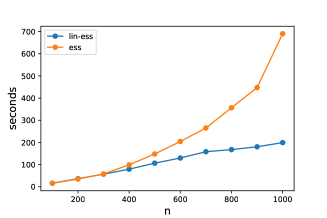
Figure 4: Computational time for sampling from the posterior of SkewGP0 using ess vs. lin-ess on a standard laptop.

The average CPU time required to compute $\Phi_{s+|B_{i}|}(\tilde{\boldsymbol{[}\gamma]}_{B_{i}};~{}\tilde{\Gamma}_{B_{i}})$ with $|B_{i}|=30$, using the randomized lattice routine with $5000$ points (Genz, 1992), is $0.5$ seconds on a standard laptop. Since the above method is randomized, we use the simultaneous perturbation stochastic approximation algorithm (Spall, 1998) for optimizing the maximum lower bound (16).

Finally notice that, both the computation of the lower bound of the marginal likelihood and the sampling from the posterior via lin-ess are highly parallelizable. In fact, each term $\Phi_{s+|B_{i}|}(\tilde{\boldsymbol{[}\gamma]}_{B_{i}};~{}\tilde{\Gamma}_{B_{i}})$ can be computed independently as well as each sample in lin-ess can be sample independently (because lin-ess is rejection-free and, therefore, no “burn in” is necessary).

6 Properties of the Posterior

In the above sections, we have shown how to compute the posterior distribution of a SkewGP process when the likelihood is a probit model. The full conjugacy of the model allows us to prove that the posterior is again a SkewGP process. This section provides more details on the properties of the posterior and compares it with two approximations. For GP classification, there are two main alternative approximation schemes for finding a Gaussian approximation to the posterior: the Laplace’s method and the Expectation-Propagation (EP) method, see, e.g. Rasmussen and Williams (2006) chapter 3.

Figure 5 provides a one-dimensional illustration using a synthetic classification problem with 50 observations and scalar inputs taken from (Kuss and Rasmussen, 2005). Figure 5(a) shows the dataset and the predictive posterior probability for the Laplace and EP approximations. Moreover, by using a SkewGP prior with latent dimension $s=0$ (that coincides with a GP prior), we have computed the exact SkewGP predictive posterior probability. Therefore, all three methods have the same prior: a GP with zero mean and RBF covariance function (the lengthscale and variance of the kernel are the same for all the three methods and have been set equal to the values that maximise the Laplace’s approximation to the marginal likelihood). Figure 5(c) shows the posterior mean latent function and corresponding 95% credible intervals. It is evident that the true posterior (SkewGP) of the latent function is skew (see for instance for $x\in[0,2]$ and the slice plot in Figure 5(b)). Laplace’s approximation peaks at the posterior mode, but places too much mass over positive values of $f$. The EP approximation aims to match the first two moments of the posterior and, therefore, usually obtains a better coverage of the posterior mass. That is why EP is usually the method of choice for approximate inference in GP classification.

Figure 6 shows the true posterior and the two approximations for the same dataset, but now the lengthscale and variance of the kernel are the optimal values for the three methods. It is evident that the skewness of the posterior provides a better model fit to the data.

Figure 7 shows the posteriors corresponding to a prior SkewGP process with latent-dimension $s=2$. The red dot denotes the optimal location of the pseudo-point $r_{1}$, while $r_{2}=13.5$ (their initial location were $5.8$ and, respectively, $6$). The additional degrees of freedom of the SkewGP prior process gave a much more satisfactory answer than that obtained from a GP prior model. By comparing Figures 6 and 7, it can be noticed that the skew-point allows us to locally modulate the skewness. Moreover, the additional degrees of freedom do not lead to overfitting, even with small data, as highlighted by the optimized location of $r_{2}$ (far away) that has not effect on the skewness of the posterior SkewGP.

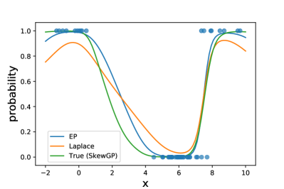
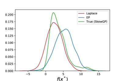
(a)	(b)

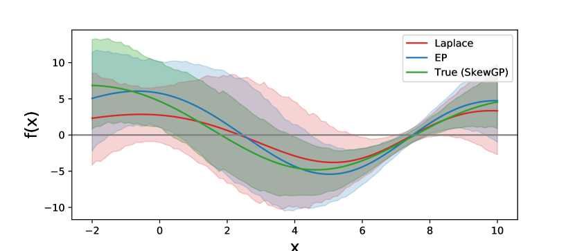
(c)

Figure 5: Plot (a) shows the training dataset and compares the true posterior mean probability of class 1, that is a SkewGP, versus the approximations computed via Laplace’s method and EP. Plot (c) shows the posterior mean latent function and corresponding 95% credible intervals for the three methods and Plot (b) reports the density-plot of the latent function posterior prediction at $x^{*}=0.42$.

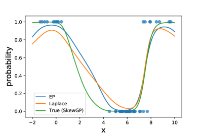
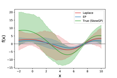
(a)	(b)

Figure 6: Plot (a) shows the training dataset and compares the true posterior mean probability of class 1, that is a SkewGP, versus the approximations computed via Laplace’s method and EP. Plot (b) shows the posterior mean latent function and corresponding 95% credible intervals for the three methods.

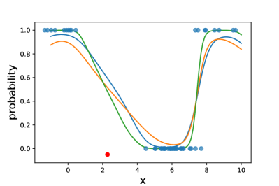
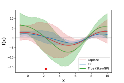
(a)	(b)

Figure 7: Plot (a) shows the training dataset and compares the true posterior mean probability of class 1, that is a SkewGP2, versus the approximations computed via Laplace’s method and EP. Plot (b) shows the posterior mean latent function and corresponding 95% credible intervals for the three methods. The red dot denotes the optimal location of the pseudo-point $r_{1}$.

7 Results

We have evaluated the proposed SkewGP classifier on a number of benchmark classification datasets and compared its classification accuracy with the accuracy of a Gaussian process classifier that uses either Laplace’s method (GP-L) or Expectation Propagation (GP-EP) for approximate Bayesian inference. For GP-L and GP-EP, we have used the implementation available in GPy (GPy, since 2012).

7.1 Penn Machine Learning Benchmarks

From the Penn Machine Learning Benchmarks (Olson et al., 2017), we have selected 124 datasets (number of features up to $500$). Since this pool includes non-binary class datasets, we have defined a binary sub-problem by considering the first (class $0$) and second (class $1$) class. The resulting binarised subset of datasets includes datasets with number of instances between $100$ and $7400$. We have scaled the inputs to zero mean and unit standard deviation and used, as performance measure, the average information in bits of the predictions about the test targets (Kuss and Rasmussen, 2005):

$$I(p_{i}^{*},y_{i})=\frac{y_{i}+1}{2}\log_{2}(p_{i}^{*})+\frac{1-y_{i}}{2}\log_{2}(1-p_{i}^{*})+1,$$

where $p_{i}^{*}$ is the predicted probability for class $1$. This score equals $1$ bit if the true label is predicted with absolute certainty, $0$ bits for random guessing and takes negative values if the prediction gives higher probability to the wrong class. We have assessed the above performance measure for the three classifiers by using 5-fold cross-validation.

While we could use any kernel for GP-L, GP-EP and SkewGP, in this experiment we have chosen the RBF kernel with a lengthscale for each dimension. Figure 8 contrasts GP-L and GP-EP with SkewGP0 (SkewGP with $s=0$) and SkewGP2 (SkewGP with $s=2$). We selected $s=2$ because we decided to use the same dimension for all datasets and, since there are several datasets where the ratio between the number of features and the number of instances is high, a latent dimension $s>2$ leads to a number of parameters that exceeds the number of instances affecting the convergence of the maximization of the marginal likelihood. The proposed SkewGP2 and SkewGP0 outperform the other two models for most data sets. The average information score of SkewGP2 is $0.573$ (average accuracy $0.904$), SkewGP0 is $0.557$ (acc. $0.882$), GP-EP is $0.542$ (acc. $0.859$) and GP-L is $0.512$ (acc. $0.863$).

This claim is supported by a statistical analysis. We have compared the three classifiers using the (nonparametric) Bayesian signed-rank test (Benavoli et al., 2014, 2017). This test declares two classifiers practically equivalent when the difference of average information is less than 0.01 (1%). The interval $[-0.01,0.01]$ thus defines a region of practical equivalence (rope) for classifiers. The test returns the posterior probability of the vector $[p(Cl_{1}>Cl_{2}),p(Cl_{1}\approx Cl_{2}),p(Cl_{1}<Cl_{2})]$ and, therefore, this posterior can be visualised in the probability simplex (Figure 9). For the comparison GP-L vs. GP-EP, as expected it can seen that GP-EP is better than GP-L. Conversely, for GP-EP versus SkewGP0, 100% of the posterior mass is in the region in favor of SkewGP0, which is the region at the right bottom of the triangle. This confirms that SkewGP0 is practically significantly better than GP-L and GP-EP. The comparison SkewGP2 versus SkewGP0 shows that SkewGP2 has surely an average information score that is not worse than that of SkewGP0 and better with probability about $0.76$.

The difference between GP-L and GP-EP, and SkewGP is that the posterior of SkewGP can be skewed. Therefore, we expect SkewGP to outperform GP-L and GP-EP on the datasets for which the posterior is far from Normal (e.g., highly skewed). To verify that we have computed the sample skewness statistics (SS) for each test input $\mathbf{x}_{i}^{*}$:

$$SS(\mathbf{x}_{i}^{*})={\frac{\operatorname{E}\left[(f(\mathbf{x}_{i}^{*})-\mu)^{3}\right]}{(\operatorname{E}\left[(f(\mathbf{x}_{i}^{*})-\mu)^{2}\right])^{3/2}}}$$

with $\mu=\operatorname{E}\left[(f(\mathbf{x}_{i}^{*})\right]$ and the expectation $\operatorname{E}[\cdot]$ can be approximated using the posterior samples drawn as in Theorem 5.1. Note that $SS(\mathbf{x}_{i}^{*})=0$ for symmetric distributions. Figure 10(left) shows, for each of the 124 datasets, the difference between the average information score of SkewGP0 and GP-EP in the y-axis, and $\max_{\mathbf{x}_{i}^{*}}SS(\mathbf{x}_{i}^{*})$ for SkewGP0 in the x-axis. We used a regression tree (green line) to detect structural changes in the mean of these data points. It is evident that, for large values of the maximum skewness statistics, SkewGP0 outperforms GP-EP (the average difference is positive). Figure 10(right) reports a similar plot for SkewGP2 and the difference is even more evident. This confirms that SkewGP on average outperforms GP-EP in those datasets where the posterior is skewed and has a similar performance otherwise.

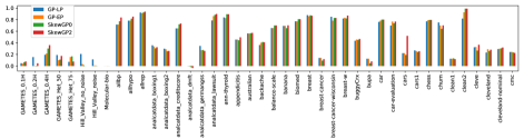
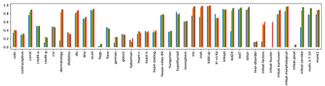
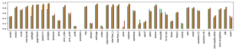
Figure 8: Average information score on 124 datasets of the Penn Machnine Learning Benchmark dataset.

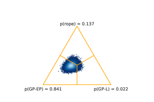
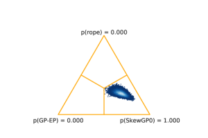
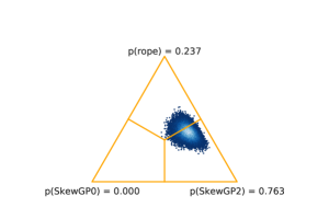
Figure 9: Bayesian Wilcoxon signed-rank test

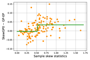
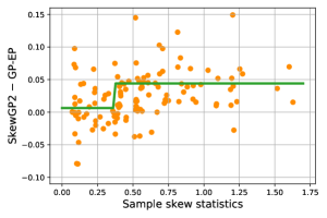
Figure 10: Maximum skewness statistics versus difference in average information score. For visualisation purpose only, we bounded the y-axis to $[-0.11,0.16]$.

7.2 Image classification

We have also considered an image classification task: Fashion MNIST dataset (each image is $28\times 28=784$ pixels and there are 10 classes: 0 T-shirt/top, 1 Trouser, 2 Pullover, 3 Dress, 4 Coat, 5 Sandal, 6 Shirt, 7 Sneaker, 8 Bag, 9 Ankle boot). We randomly pooled 10000 images from the dataset and divided them into two sets, with 5000 cases for training and 5000 for testing. For each one of the 10 classes, we have defined a binary classification sub-problem by considering one class against all the other classes. We have compared GP-EP and SkewGP2, that is a SkewGP with latent dimension $s=2$ (for the same reason outlined in the previous section). We have initialised $r_{i}$ by taking $2$ random samples from the training data. We have also considered two different kernels: RBF and the Neural Network kernel (Williams, 1998). Table 2 reports the accuracy for each of the 10 binary classification sub-problems. For the RBF kernel, it can be noticed that SkewGP2 outperforms GP-EP in all sub-problems. For the NN kernel, the differences between the two models are less substantial (due to the higher performance of the NN kernel on this dataset) but in any case in favor of SkewGP2. We have also reported, for both the models, the computational time (in minutes) needed to optimize the hyperparameters, to compute the posterior and to compute the predictions for all instances in the test set. This shows that SkewGP2 is also faster than GP-EP. The last row reports the accuracy on the original multi-class classification problem obtained by using the one-vs-rest heuristic, with the only goal of showing that the more accurate estimate of the probability by SkewGP leads also to an increase in accuracy for one-vs-rest. A multi-class Laplace’s approximation for GP classification was developed by Williams and Barber (1998) and other implementations are for instance discussed by Hernández-Lobato et al. (2011) and Chai (2012), we plan to address multi-class classification in future work.

	RBF kernel		NN kernel
	Accuracy		Accuracy		Time
Class	GP-EP	SkewGP2	GP-EP	SkewGP2	GP-EP	SkewGP2
0	0.945	0.955	0.956	0.958	80.7	67.8
1	0.988	0.990	0.988	0.991	125.7	68.0
2	0.923	0.934	0.943	0.943	130.9	70.7
3	0.951	0.961	0.953	0.961	79.2	56.9
4	0.932	0.946	0.946	0.944	121.1	49.3
5	0.967	0.980	0.975	0.983	110.5	53.0
6	0.917	0.922	0.924	0.933	115.7	65.1
7	0.970	0.974	0.981	0.983	113.6	66.3
8	0.969	0.979	0.980	0.981	121.5	51.4
9	0.980	0.982	0.983	0.986	137.0	55.0
One-vs-rest	0.785	0.821	0.823	0.844

Table 1: Image classification

Our goal is assessing the accuracy but also the quality of the probabilistic predictions. Figure 12, plot (a1), shows, for the RBF kernel case and for each instance in the test set of the binary sub-problem relative to class 8 vs. rest, the value of of the mean predicted probability of class rest for SkewGP2 (x-axis) and GP-EP (y-axis). Each instance is represented as a blue point. The red points highlight the instances that were misclassified by GP-EP. Figure (a2) shows the same plot, but the red points are now the instances that were misclassified by SkewGP2. By comparing (a1) and (a2), it is evident that SkewGP2 provides a higher quality of the probabilistic predictions.

SkewGP2 also returns a better estimate of its own uncertainty. This is showed in plots (b1) vs. (b2). For each instance in the test set and for each sample from the posterior, we have computed the predicted class (the class that has probability greater than $0.5$). For each test instance, we have then computed the standard deviation of all these predictions and used it to color the scatter plot of the mean predicted probability. In this way, we have a visual representation of first order (mean predicted probability) and second order (standard deviation of the predictions) uncertainty. Plot 12(b1) is relative to GP-EP and shows that GP-EP confidence is low only for the instances whose mean predicted probability is close to $0.5$. This is not reflected in the value of the mean predicted probability for the misclassified instances (compare plot (a1) and (b1)). We have also computed the histogram of the standard deviation of the predictions for those instances that were misclassified by GP-EP in Figure (c1). Note that, the peak of the histogram corresponds to very low standard deviation, that means GP-EP has misclassified instances that have low second order uncertainty. This implies that the model is overestimating its confidence. Conversely, the second order uncertainty of SkewGP2 is clearly consistent, see plot (a2) and (b2), and in particular the histogram in (c2) – the peak is in correspondence of high values of the standard deviation of the predictions. In other words, SkewGP2 has mainly misclassified instances with high second order uncertainty, that is what we expect from a calibrated probabilistic model. We have reported additional examples of the better calibration of SkewGP2 for the MNIST and German-road sign dataset in appendix.

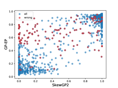
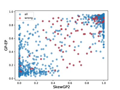
(a1)	(a2)
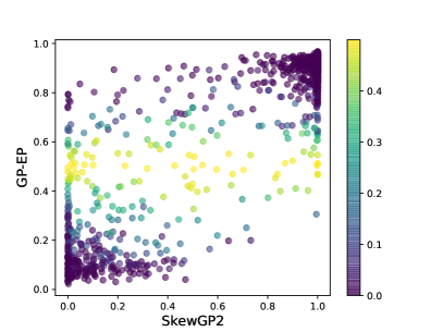
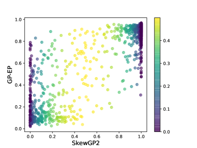
(b1)	(b2)
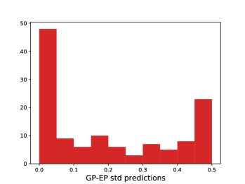
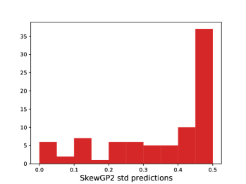
(c1)	(c2)

Figure 11: Fashion MNIST dataset

8 Conclusions

We have introduced the Skew Gaussian process (SkewGP) as an alternative to Gaussian processes for classification. We have shown that SkewGP and the probit likelihood are conjugate and provided marginals and closed form conditionals. We have also shown that SkewGP contains the GP as a special case and, therefore, SkewGPs inherit all good properties of GPs and increase their flexibility. The SkewGP prior was applied in classification showing improved performance over GPs (Laplace’s method and Expectation Propagation approximations).

As future work, we plan to study other more native ways to parametrize the skewness matrix $\Delta$ that do not rely on an underlying kernel. Moreover, we plan to investigate the possibility of using inducing points, as for sparse GPs, to reduce the computational load for matrix operations (complexity $O(n^{3})$ with storage demands of $O(n^{2})$) as well as deriving the posterior for the multi-class classification problem.

Appendix A Proofs

Proposition 1

To prove that, we exploit Kolmogorov’s extension theorem (Orbanz, 2009). Suppose that a family $\mathcal{F}^{I}$ of probability measures are the I-finite-dimensional marginals of an infinite-dimensional measure $\mathcal{F}$ (a “stochastic process”). Each measure $\mathcal{F}^{I}$ belongs to the finite-dimensional subspace of dimension $I$. Given two marginals $\mathcal{F}^{I},\mathcal{F}^{J}$, as marginals of the same measure $\mathcal{F}$, they must be marginals of each other, that is

$$\mathcal{F}^{I}=\mathcal{F}^{J\downarrow I}\text{ whether }I\subset J,$$ (17)

where $\cdot\downarrow I$ denotes the projection onto the subspace of dimension $I$. A family of probability measures that satisfies (17) is called a projective family. The Kolmogorov’s extension theorem states that any projective family on the finite-dimensional subspaces of an infinite-dimensional product space uniquely defines a stochastic process on the space. This means that we can define a nonparametric Bayesian model from a finite-dimensional distribution by simply verifying that (17) holds. From (3), it then immediately follows that the definition (5) uniquely defines a stochastic process and, therefore, SkewGP is a well-defined stochastic process.

Theorem 3.1

We aim to derive the posterior of $f(X)$. The joint distribution of $f(X),\mathcal{D}$ is

$$p(\mathcal{D}|f(X))p(f(X))$$

$$=\Phi_{n}(W\boldsymbol{[}f];I_{n})\;\text{SUN}_{n,s}(\boldsymbol{[}\xi],\Omega,\Delta,\boldsymbol{[}\gamma],\Gamma)$$

$$=\Phi_{n}(W\boldsymbol{[}f];I_{n})\;\phi_{n}(\boldsymbol{[}f]-\boldsymbol{[}\xi];\Omega)\frac{\Phi_{s}\left(\boldsymbol{[}\gamma]+\Delta^{T}\bar{\Omega}^{-1}D_{\Omega}^{-1}(\boldsymbol{[}f]-\boldsymbol{[}\xi]);\Gamma-\Delta^{T}\bar{\Omega}^{-1}\Delta\right)}{\Phi_{s}\left(\boldsymbol{[}\gamma];\Gamma\right)}$$

$$\propto\phi_{n}(\boldsymbol{[}f]-\boldsymbol{[}\xi];\Omega)\Phi_{n}(W\boldsymbol{[}f];I_{n})\Phi_{s}\left(\boldsymbol{[}\gamma]+\Delta^{T}\bar{\Omega}^{-1}D_{\Omega}^{-1}(\boldsymbol{[}f]-\boldsymbol{[}\xi]);\Gamma-\Delta^{T}\bar{\Omega}^{-1}\Delta\right)$$ (18)

where we denoted $\boldsymbol{[}f]=f(X)\in\mathbb{R}^{n}$ and omitted the dependence on $X$. First, note that

$$\Phi_{n}(W\boldsymbol{[}f];I_{n})$$

$$=\Phi_{n}\left(W\boldsymbol{[}\xi]+(\bar{\Omega}D_{\Omega}W^{T})^{T}\bar{\Omega}^{-1}D_{\Omega}^{-1}(\boldsymbol{[}f]-\boldsymbol{[}\xi]);(W\Omega W^{T}+I_{n})-WD_{\Omega}\bar{\Omega}D_{\Omega}W^{T}\right)$$

Therefore, we can write

$$\Phi_{n}(W\boldsymbol{[}f];I_{n})\Phi_{s}\left(\boldsymbol{[}\gamma]+\Delta^{T}\bar{\Omega}^{-1}D_{\Omega}^{-1}(\boldsymbol{[}f]-\boldsymbol{[}\xi]);\Gamma-\Delta^{T}\bar{\Omega}^{-1}\Delta\right)$$

$$=\Phi_{n}\left(W\boldsymbol{[}\xi]+(\bar{\Omega}D_{\Omega}W^{T})^{T}\bar{\Omega}^{-1}D_{\Omega}^{-1}(\boldsymbol{[}f]-\boldsymbol{[}\xi]);(W\Omega W^{T}+I_{n})-WD_{\Omega}\bar{\Omega}D_{\Omega}W^{T}\right)$$

$$\cdot\Phi_{s}\left(\boldsymbol{[}\gamma]+\Delta^{T}\bar{\Omega}^{-1}D_{\Omega}^{-1}(\boldsymbol{[}f]-\boldsymbol{[}\xi]);\Gamma-\Delta^{T}\bar{\Omega}^{-1}\Delta\right)$$

$$=\Phi_{s+n}(m;M)$$ (19)

with

$$m=\begin{bmatrix}\boldsymbol{[}\gamma]+\Delta^{T}\bar{\Omega}^{-1}D_{\Omega}^{-1}(\boldsymbol{[}f]-\boldsymbol{[}\xi])\\ W\boldsymbol{[}\xi]+(\bar{\Omega}D_{\Omega}W^{T})^{T}\bar{\Omega}^{-1}D_{\Omega}^{-1}(\boldsymbol{[}f]-\boldsymbol{[}\xi])\end{bmatrix},$$

and

$$M=\begin{bmatrix}\Gamma-\Delta^{T}\bar{\Omega}^{-1}\Delta&0\\ 0&(W\Omega W^{T}+I_{n})-WD_{\Omega}\bar{\Omega}D_{\Omega}W^{T}\end{bmatrix}.$$

From (18)–(19) and the definition of the PDF of the SUN distribution (1), we can easily show that we can rewrite (18) as a SUN distribution with updated parameters:

$$\tilde{\xi} =\xi,$$

$$\tilde{\Omega} =\Omega,$$

$$\tilde{\Delta} =[\Delta,~{}~{}\bar{\Omega}D_{\Omega}W^{T}],$$

$$\tilde{\boldsymbol{[}\gamma]} =[\boldsymbol{[}\gamma],~{}~{}W\xi]^{T},$$

$$\tilde{\Gamma} =\begin{bmatrix}\Gamma&\quad\Delta^{T}D_{\Omega}W^{T}\\ WD_{\Omega}\Delta&\quad(W\Omega W^{T}+I_{n})\end{bmatrix}.$$

Corollary 1

This follows directly from the above proof by observing that $\Phi_{s+n}(\tilde{\boldsymbol{[}\gamma]},\tilde{\Gamma})$ is the normalization constant of the posterior and, therefore, the marginal likelihood is

$$\frac{\Phi_{s+n}(\tilde{\boldsymbol{[}\gamma]},\tilde{\Gamma})}{\Phi_{s}(\boldsymbol{[}\gamma],\Gamma)}.$$

Corollary 2

Denote with $\hat{f}(\hat{X})=[f(X)^{T},f({\boldsymbol{[}x]^{*}})^{T}]^{T}$ and observe that the predictive distribution is by definition

$$\int\int\Phi(f^{*};1)p(f^{*}|\boldsymbol{[}f])p(\boldsymbol{[}f]|\mathcal{D})d\boldsymbol{[}f]df^{*},$$

with $f^{*}:=f({\boldsymbol{[}x]^{*}})$ and $\boldsymbol{[}f]=f(X)$. Note that we have omitted the dependence on $\boldsymbol{[}x]^{*},X$ for easier notation ($p(f^{*}|\boldsymbol{[}f])$ corresponds to $p(f^{*}|\boldsymbol{[}x]^{*},X,\boldsymbol{[}f])$). We can write the posterior as

$$p(\boldsymbol{[}f]|\mathcal{D})=\dfrac{p(\mathcal{D}|\boldsymbol{[}f])p(\boldsymbol{[}f])}{p(\mathcal{D})},$$

and so

$$\int\int\Phi(f^{*};1)p(f^{*}|f)p(\boldsymbol{[}f]|\mathcal{D})d\boldsymbol{[}f]df^{*}$$

$$=\dfrac{1}{p(\mathcal{D})}\int\int\Phi(f^{*};1)p(f^{*}|\boldsymbol{[}f])p(\mathcal{D}|\boldsymbol{[}f])p(\boldsymbol{[}f])d\boldsymbol{[}f]df^{*}$$

$$=\dfrac{1}{p(\mathcal{D})}\int\int\Phi(f^{*};1)p(\mathcal{D}|\boldsymbol{[}f])p(\boldsymbol{[}f],f^{*})d\boldsymbol{[}f]df^{*}.$$

Observe that

$$\Phi(f^{*};1)p(\mathcal{D}|\boldsymbol{[}f])=\Phi(f^{*};1)\Phi_{n}(W\boldsymbol{[}f];I_{n})=\Phi_{n+1}(\hat{W}\hat{f};I_{n+1})$$

with $\hat{W}=\text{diag}(2y_{1}-1,\dots,2y_{n+1}-1)$ and $y_{n+1}=0.5$. Note that $2y_{n+1}-1=2\cdot 0.5-1=0$ and this is the reason why we have introduced the dummy class value $1/2$.

Observe that

$$\int\int\Phi_{n+1}(\hat{W}\hat{f};I_{n+1})p(\boldsymbol{[}f],f^{*})d\boldsymbol{[}f]df^{*}$$

is the marginal likelihood of a SkewGP posterior corresponding to the augmented dataset $\hat{X}=[X^{T},{\boldsymbol{[}x]^{*}}^{T}]^{T}$, $\hat{y}=[y^{T},1/2]^{T}$. Therefore, we have that

$$\frac{1}{p(\mathcal{D})}\int\int\Phi_{n+1}(\hat{W}\hat{f};I_{n+1})p(\boldsymbol{[}f],f^{*})d\boldsymbol{[}f]df^{*}=\dfrac{\frac{\Phi_{s+n+1}(\tilde{\boldsymbol{[}\gamma]}^{*},\tilde{\Gamma}^{*})}{\Phi_{s}(\boldsymbol{[}\gamma],\Gamma)}}{\frac{\Phi_{s+n}(\tilde{\boldsymbol{[}\gamma]},\tilde{\Gamma})}{\Phi_{s}(\boldsymbol{[}\gamma],\Gamma)}},$$

where $\tilde{\boldsymbol{[}\gamma]}^{*},\tilde{\Gamma}^{*}$ are the corresponding matrices of the posterior computed for the augmented dataset.

Proposition 2

This follows by the Fréchet inequality:

$$Pr(A_{1},A_{2},\dots,A_{b})\geq\max\left(0,\sum_{i=1}^{b}Pr(A_{i})-(b-1)\right),$$

where $A_{i}$ are events. In fact, note that

$$\Phi_{s+n}(\tilde{\boldsymbol{[}\gamma]};\tilde{\Gamma})=Pr(u_{1}\geq\tilde{\boldsymbol{[}\gamma]}_{1},\dots,u_{s+n}\geq\tilde{\boldsymbol{[}\gamma]}_{s+n})$$

where $Pr$ is computed w.r.t. the PDF of a multivariate distribution with zero mean and covariance $\tilde{\Gamma}$.

Theorem 5.1

The proof follows straightforwardly from that of Corollary 2.

A.1 Additional image classification examples

We have defined a binary sub-problem from the German Traffic Sign data by considering Speed-Limit 30 vs. 50 and from MNIST digit dataset by considering 3 vs. 5. We have compared GP-L vs. SkewGP₂ (both with RBF kernel). Table 2 reports the average accuracy and shows again SkewGP₂ outperforms GP-L (GP-EP achieves lower accuracy than GP-L in both cases).

Dataset	classes	GP-L	SkewGP2
German Traffic Sign	Speed-Limit 30 vs. 50	0.96	0.98
MNIST	3 vs. 5	0.80	0.90

Table 2: Image classification

Our goal is assessing the accuracy but also the quality of the probabilistic predictions. Figure 12, plot (a1), shows, for each instance in the test set (one of the fold) of the MNIST datatset , the value of of the mean predicted probability of class $5$ for SkewGP₂ (x-axis) and GP-L (y-axis). Each instance is represented as a blue point. The mean predicted probability ranges in $[0.41,0.53]$ for GP-L and in $[0.25,0.8]$ for SkewGP₂. The red points highlight the instances that were misclassified by GP-L (plot (a2) reports the images of some of the misclassified instances included in the rectangle). Figure (b1) shows the same plot, but the red points are now the instances that were misclassified by SkewGP₂. By comparing (a) and (b), it is evident that SkewGP₂ provides a higher quality of the probabilistic predictions.

SkewGP₂ also returns a better estimate of its own uncertainty. This is showed in plots (c1) and (c2). For each instance in the test set and for each sample from the posterior, we have computed the predicted class (the class that has probability greater than $0.5$). For each test instance, we have then computed the standard deviation of all these predictions and used it to color the scatter plot of the mean predicted probability. In this way, we have a visual representation of first order (mean predicted probability) and second order (standard deviation of the predictions) uncertainty. Plot 12(c1) is relative to GP-L and shows that GP-L confidence is low only for the instances whose mean predicted probability is close to $0.5$. This is not reflected in the value of the mean predicted probability for the misclassified instances (compare plot (a1) and (c1) and note that the red spot in (a1) is outside the yellow area in (c1)). Conversely, the second order uncertainty of SkewGP₂ is clearly consistent with plot (b1).

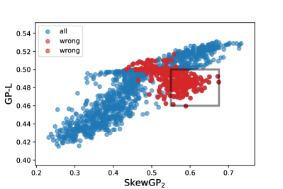
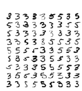
(a1)	(a2)
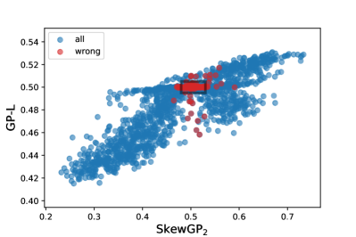
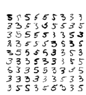
(b1)	(b2)
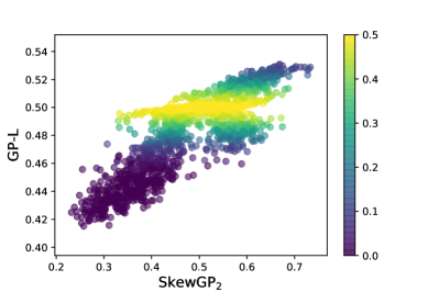
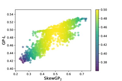
(c1)	(c2)

Figure 12: MNIST dataset

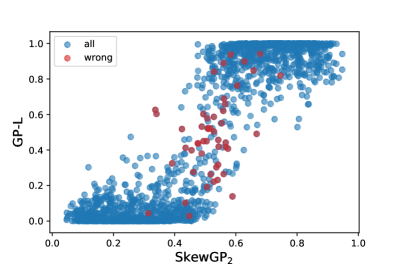
(a1)	(a2)
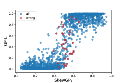
(b1)	(b2)
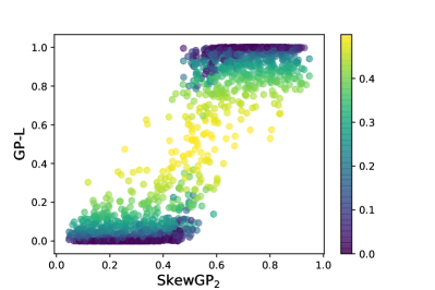
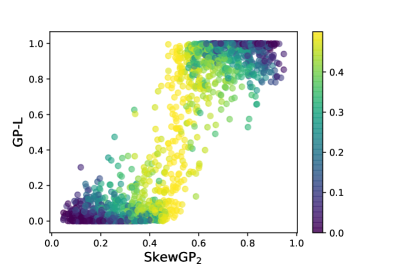
(c1)	(c2)

Figure 13: German-road sign dataset

Figure 13 shows a similar plot for the “German road-sign” dataset. Plot 13(c1) is relative to GP-L and shows that GP-L confidence is low only for the instances whose mean predicted probability is in $[0.3,0.7]$. This is not reflected in the value of the mean predicted probability for the misclassified instances (compare plot (a1) and (c1) and note that some of the red points in (a1) are outside the yellow area in (c1)). Conversely, 13(c2) shows that the second order uncertainty of SkewGP₂ is clearly consistent with plot (b1).

References

- Arellano and Azzalini (2006) Arellano RB, Azzalini A (2006) On the unification of families of skew-normal distributions. Scandinavian Journal of Statistics 33(3):561–574
- Azzalini (2013) Azzalini A (2013) The skew-normal and related families, vol 3. Cambridge University Press
- Azzimonti and Ginsbourger (2018) Azzimonti D, Ginsbourger D (2018) Estimating orthant probabilities of high-dimensional gaussian vectors with an application to set estimation. Journal of Computational and Graphical Statistics 27(2):255–267
- Bauer et al. (2016) Bauer M, van der Wilk M, Rasmussen CE (2016) Understanding probabilistic sparse gaussian process approximations. In: Advances in neural information processing systems, pp 1533–1541
- Benavoli et al. (2014) Benavoli A, Mangili F, Corani G, Zaffalon M, Ruggeri F (2014) A Bayesian Wilcoxon signed-rank test based on the Dirichlet process. In: Proceedings of the 30th International Conference on Machine Learning (ICML 2014), pp 1–9
- Benavoli et al. (2017) Benavoli A, Corani G, Demsar J, Zaffalon M (2017) Time for a change: a tutorial for comparing multiple classifiers through Bayesian analysis. Journal of Machine Learning Research 18(77):1–36
- Botev (2017) Botev ZI (2017) The normal law under linear restrictions: simulation and estimation via minimax tilting. Journal of the Royal Statistical Society: Series B (Statistical Methodology) 79(1):125–148
- Chai (2012) Chai KMA (2012) Variational multinomial logit gaussian process. Journal of Machine Learning Research 13(Jun):1745–1808
- Durante (2018) Durante D (2018) Conjugate Bayes for probit regression via unified skew-normals. arXiv preprint arXiv:180209565
- Fang (2018) Fang KW (2018) Symmetric multivariate and related distributions. Chapman and Hall/CRC
- Genton et al. (2018) Genton MG, Keyes DE, Turkiyyah G (2018) Hierarchical decompositions for the computation of high-dimensional multivariate normal probabilities. Journal of Computational and Graphical Statistics 27(2):268–277
- Genz (1992) Genz A (1992) Numerical computation of multivariate normal probabilities. Journal of computational and graphical statistics 1(2):141–149
- Genz and Bretz (2009) Genz A, Bretz F (2009) Computation of multivariate normal and t probabilities, vol 195. Springer Science & Business Media
- Gessner et al. (2019) Gessner A, Kanjilal O, Hennig P (2019) Integrals over gaussians under linear domain constraints. arXiv preprint arXiv:191009328
- GPy (since 2012) GPy (since 2012) GPy: A gaussian process framework in python. http://github.com/SheffieldML/GPy
- Hernández-Lobato et al. (2011) Hernández-Lobato D, Hernández-Lobato JM, Dupont P (2011) Robust multi-class gaussian process classification. In: Advances in neural information processing systems, pp 280–288
- Kuss and Rasmussen (2005) Kuss M, Rasmussen CE (2005) Assessing approximate inference for binary Gaussian process classification. Journal of machine learning research 6(Oct):1679–1704
- Murray et al. (2010) Murray I, Adams R, MacKay D (2010) Elliptical slice sampling. In: Teh YW, Titterington M (eds) Proceedings of the Thirteenth International Conference on Artificial Intelligence and Statistics, PMLR, Chia Laguna Resort, Sardinia, Italy, Proceedings of Machine Learning Research, vol 9, pp 541–548
- Nickisch and Rasmussen (2008) Nickisch H, Rasmussen CE (2008) Approximations for binary gaussian process classification. Journal of Machine Learning Research 9(Oct):2035–2078
- O’Hagan (1991) O’Hagan A (1991) Bayes–hermite quadrature. Journal of statistical planning and inference 29(3):245–260
- O’Hagan and Leonard (1976) O’Hagan A, Leonard T (1976) Bayes estimation subject to uncertainty about parameter constraints. Biometrika 63(1):201–203
- Olson et al. (2017) Olson RS, La Cava W, Orzechowski P, Urbanowicz RJ, Moore JH (2017) PMLB: a large benchmark suite for machine learning evaluation and comparison. BioData Mining 10(1):36, DOI 10.1186/s13040-017-0154-4, URL https://doi.org/10.1186/s13040-017-0154-4
- Orbanz (2009) Orbanz P (2009) Construction of nonparametric Bayesian models from parametric Bayes equations. In: Advances in neural information processing systems, pp 1392–1400
- Phinikettos and Gandy (2011) Phinikettos I, Gandy A (2011) Fast computation of high-dimensional multivariate normal probabilities. Computational Statistics & Data Analysis 55(4):1521–1529
- Quiñonero-Candela and Rasmussen (2005) Quiñonero-Candela J, Rasmussen CE (2005) A unifying view of sparse approximate gaussian process regression. Journal of Machine Learning Research 6(Dec):1939–1959
- Rasmussen and Williams (2006) Rasmussen CE, Williams CK (2006) Gaussian processes for machine learning. MIT press Cambridge, MA
- Snelson and Ghahramani (2006) Snelson E, Ghahramani Z (2006) Sparse Gaussian processes using pseudo-inputs. In: Advances in neural information processing systems, pp 1257–1264
- Spall (1998) Spall JC (1998) Implementation of the simultaneous perturbation algorithm for stochastic optimization. IEEE Transactions on aerospace and electronic systems 34(3):817–823
- Titsias (2009) Titsias M (2009) Variational learning of inducing variables in sparse gaussian processes. In: van Dyk D, Welling M (eds) Proceedings of the Twelth International Conference on Artificial Intelligence and Statistics, PMLR, Hilton Clearwater Beach Resort, Clearwater Beach, Florida USA, Proceedings of Machine Learning Research, vol 5, pp 567–574
- Williams (1998) Williams CK (1998) Computation with infinite neural networks. Neural Computation 10(5):1203–1216
- Williams and Barber (1998) Williams CK, Barber D (1998) Bayesian classification with gaussian processes. IEEE Transactions on Pattern Analysis and Machine Intelligence 20(12):1342–1351
- Zhang et al. (2007) Zhang Z, Wu G, Chang EY (2007) Semiparametric Regression Using Student Processes. IEEE Transactions on Neural Networks 18(6):1572–1588