Stability Assessment of Stochastic Differential-Algebraic Systems via Lyapunov Exponents with an Application to Power Systems

Abstract

In this paper we discuss Stochastic Differential-Algebraic Equations (SDAEs) and the asymptotic stability assessment for such systems via Lyapunov exponents (LEs). We focus on index-one SDAEs and their reformulation as ordinary stochastic differential equation (SDE). Via ergodic theory it is then feasible to analyze the LEs via the random dynamical system generated by the underlying SDE. Once the existence of well-defined LEs is guaranteed, we proceed to the use of numerical simulation techniques to determine the LEs numerically. Discrete and continuous $QR$ decomposition-based numerical methods are implemented to compute the fundamental solution matrix and to use it in the computation of the LEs. Important computational features of both methods are illustrated via numerical tests. Finally, the methods are applied to two applications from power systems engineering, including the single-machine infinite-bus (SMIB) power system model.

Keywords: Stochastic Differential-Algebraic Equations, Lyapunov exponent, Power system stability, Spectral analysis, Stochastic systems, Numerical methods.

1 Introduction

Modeling the dynamic behavior of systems employing differential-algebraic equations is a mathematical representation paradigm widely used in many areas of science and engineering. On the other hand, the dynamics of systems perturbed by stochastic processes have been adequately modeled by stochastic differential equations (SDEs). The need of a generalized concept which covers both DAEs and SDEs, and allows the modeling and analysis of constrained systems subjected to stochastic disturbances, has led to the formulation of stochastic differential-algebraic equations (SDAEs). While there has been a broad and fruitful development both in the field of DAEs and SDEs (see, e.g. [6, 7, 23] and [20, 30, 32], respectively), studies of the concepts and the numerical treatment of SDAEs are rather limited, see e.g. [10, 37, 42]. The main reason for this is that the proper treatment of algebraic constraints in SDAEs faces many difficulties, except in the case that all the constraints are explicitly given and can be resolved during the numerical integration process, which is the case that we will discuss.

As tool for the stability analysis we use Lyapunov exponents (LEs) introduced as characteristic exponents in [28]. The theory of LEs experienced a crucial development with the work [33] which, via the Multiplicative Ergodic Theorem (MET), ensures the regularity and existence of the LEs belonging to a linear cocycle over a metric dynamical system, see [3] for a detailed presentation of the theory. We review and extend the main concepts of this approach for asymptotic stability assessment of differential-algebraic equations driven by Gaussian white noise and apply the technique in the setting of power systems.

Following the ideas from [10, 11, 24, 37, 42], properties such as the existence and uniqueness of solutions are reviewed. Analogously to the DAE case, we define the class of strangeness-free (index-one) SDAEs and show that SDAE systems with this structure can be reduced to a classical SDE system that describes the dynamics of the original SDAE for which the MET can be applied to define the LEs of the system.

Once we have extended the theoretical framework that guaratees the existence of well-defined LEs, we study numerical methods, based on the $QR$ factorization of the fundamental solution matrix, that allow the numerical computation of spectral values asociated to the Lyapunov spectra. The first technique requires computing the fundamental solution matrix and forming an orthogonal factorization, while the second one involves performing a continuous $QR$ decomposition of the fundamental solution matrix. Both techniques have been extensively studied in deterministic ODE and DAE systems, see [4, 5, 15, 14, 26, 27]. This paper follows the ideas exposed in [9], where these $QR$ methods were extended to the stochastic case.

Finally, these concepts and computational techniques are used to assess the asymptotic stability of power systems affected by stochastic fluctuations. We illustrate the results with elementary test cases such as a single-machine infinite-bus system.

The paper is organized as follows: In Section 2 we recall the main theory of strangeness-free SDAEs, their relation with the SDEs, and the existence of LEs generated by such SDEs. Section 3 presents the discrete and continuous $QR$-based decomposition methods and their evaluation. Interesting study-cases in the power systems area are presented in Section 4. We finish with some conclusions in Section 5.

2 Review of the theory

2.1 Stochastic Differential-Algebraic Equations

Consider a system of quasi-linear stochastic differential-algebraic equations (SDAEs) of the form

$$\boldsymbol{E}d\boldsymbol{x}_{t}=\boldsymbol{f}_{0}(\boldsymbol{x}_{t})dt+\sum_{j=1}^{m}\boldsymbol{f}_{j}(\boldsymbol{x}_{t})dw_{t}^{j},\quad t\in\mathbb{I}:=[t_{0},t_{f}],$$ (1)

with a singular matrix $\boldsymbol{E}\in\mathbb{R}^{n\times n}$ of rank $d<n$. The function $\boldsymbol{f}_{0}\in\mathcal{C}^{k}(\mathbb{D}_{\boldsymbol{x}},\mathbb{R}^{n})$ (for some $k\geq 1$) is known as drift, and $\boldsymbol{f}_{1},\ldots,\boldsymbol{f}_{m}\in\mathcal{C}^{k+1}(\mathbb{D}_{\boldsymbol{x}},\mathbb{R}^{n})$ are the diffusions, here $\mathbb{D}_{\boldsymbol{x}}\subseteq\mathbb{R}^{n}$ is an open set. Furthermore, $w_{t}^{j}$ (for $j=1,\ldots,m$) form an $m$-dimensional Wiener process defined on the complete probability space $(\Omega,\mathcal{F},\mathbb{P})$ with a filtration $(\mathcal{F}_{t})_{t\geq t_{0}}$. Each $j$-th Wiener process is understood as a process with independent increments such that $(w_{t}-w_{s})\sim\mathcal{N}(0,t-s)$, i.e. is a Gaussian random variable for all $0\leq s<t$, such that

$$w_{0}=0,\quad\mathbb{E}[w_{t}-w_{s}]=0,\quad\mathbb{E}[w_{t}-w_{s}]^{2}=t-s.$$

Since the Wiener process is nowhere differentiable, it is more convenient to represent equation (1) in its integral form as

$$\boldsymbol{E}\boldsymbol{x}_{t}=\boldsymbol{E}\boldsymbol{x}_{t_{0}}+\int_{t_{0}}^{t}\boldsymbol{f}_{0}(\boldsymbol{x}_{s})ds+\sum_{j=1}^{m}\int_{t_{0}}^{t}\boldsymbol{f}_{j}(\boldsymbol{x}_{s})dw_{s}^{j},\quad t\in\mathbb{I}.$$ (2)

Here, the first integral is a stochastic Riemann-Stieltjes integral, and the second one is a stochastic Itô-type integral, see e.g. [32].

We assume consistent initial values $\boldsymbol{x}_{t_{0}}=\boldsymbol{x}_{0}$ independent of the Wiener processes $w_{t}^{j}$ and with finite second moments [32]. A solution $\boldsymbol{x}_{t}=\boldsymbol{x}(t,\omega)$ of (2) is an $n$-dimensional vector-valued Markovian stochastic process depending on $t\in\mathbb{I}$ and $\omega\in\Omega$ (the parameter $\omega$ is commonly omitted in the notation of $\boldsymbol{x}$). Such a solution can be defined as strong solution if it fulfills the following conditions, see e.g. [11, 42].

• $\boldsymbol{x}(\cdot)$ is adapted to the filtration $(\mathcal{F}_{t})_{t\geq t_{0}}$,

• $\int_{t_{0}}^{t_{f}}|f_{0}^{\ell}(x_{s})|ds<\infty$ almost sure (a.s.), for all $\ell=1,\ldots,n$,

• $\int_{t_{0}}^{t_{f}}|f_{j}^{\ell}(x_{s})|^{2}dw_{s}^{j}<\infty$ a.s., for all $j=1,\ldots,m$, and $\ell=1,\ldots,n$,

• (2) holds for every $t\in\mathbb{I}$ a.s.

Because of the presence of the algebraic equations associated with the kernel of $\boldsymbol{E}$, the solution components associated with these equations would be directly affected by white noise and not integrated. In order to avoid this, a reasonable restriction is to ensure that the noise sources do not appear in the algebraic constraints. According to [37, 42], this assumption can be accomplished in SDAE systems whose deterministic part

$$\boldsymbol{E}\dot{\boldsymbol{x}}_{t}=\boldsymbol{f}_{0}(\boldsymbol{x}_{t}),\quad t\in\mathbb{I},$$ (3)

is a DAE with tractability index one [25, 42], in which the constraints are regularly and globally uniquely solvable for parts of the solution vector. We slightly modify this assumption and consider SDAE systems whose deterministic part (3) is a regular strangeness-free DAE [23] i.e. it has differentiation index one. A system with these characteristics can be transformed into a semi-explicit form by means of an appropriate kinematic equivalence transformation [26, 6], i.e., there exist pointwise orthogonal matrix functions $\boldsymbol{\mathcal{P}}$ and $\boldsymbol{\mathcal{Q}}$ such that, pre-multiplying (1) by $\boldsymbol{\mathcal{P}}$, and changing the variables $\boldsymbol{x}_{t}$ according to the transformation $\boldsymbol{x}_{t}=\boldsymbol{\mathcal{Q}}\hat{\boldsymbol{x}}_{t}$ one obtains a system in semi-explicit form

$$d\hat{\boldsymbol{x}}_{t}^{D} =\hat{\boldsymbol{f}}_{0}^{D}(\hat{\boldsymbol{x}}_{t}^{D},\hat{\boldsymbol{x}}_{t}^{A})dt+\sum_{j=1}^{m}\hat{\boldsymbol{f}}_{j}^{D}(\hat{\boldsymbol{x}}_{t}^{D},\hat{\boldsymbol{x}}_{t}^{A})dw_{t}^{j},$$ (4a)

$$0 =\hat{\boldsymbol{f}}_{0}^{A}(\hat{\boldsymbol{x}}_{t}^{D},\hat{\boldsymbol{x}}_{t}^{A})dt+\sum_{j=1}^{m}\hat{\boldsymbol{f}}_{j}^{A}(\hat{\boldsymbol{x}}_{t}^{D},\hat{\boldsymbol{x}}_{t}^{A})dw_{t}^{j},$$ (4b)

where $\hat{\boldsymbol{x}}_{t}^{D}$ and $\hat{\boldsymbol{x}}_{t}^{A}$ is a separation of the transformed state into differential and algebraic variables, respectively, that is performed in such a way that the Jacobian of the function $\hat{\boldsymbol{f}}_{0}^{A}$ with respect to the algebraic variables is nonsingular, see [23] for details of the construction. The condition that the noise sources do not appear in the constraints, implies that $\sum_{j=1}^{m}\hat{\boldsymbol{f}}_{j}^{A}\equiv 0$, so that the algebraic equations in (4b) can be solved as $\hat{\boldsymbol{x}}_{t}^{A}=\boldsymbol{F}^{A}(\hat{\boldsymbol{x}}_{t}^{D})$ and inserted in the dynamic equations (4a) yielding an ordinary SDE

$$d\hat{\boldsymbol{x}}_{t}^{D} =\hat{\boldsymbol{f}}_{0}^{D}(\hat{\boldsymbol{x}}_{t}^{D},\boldsymbol{F}^{A}(\hat{\boldsymbol{x}}_{t}^{D}))dt+\sum_{j=1}^{m}\hat{\boldsymbol{f}}_{j}^{D}(\hat{\boldsymbol{x}}_{t}^{D},\boldsymbol{F}^{A}(\hat{\boldsymbol{x}}_{t}^{D}))dw_{t}^{j}.$$ (5)

This equation is called underlying SDE of the strangeness-free SDAE. It acts in the lower-dimensional subspace $\mathbb{R}^{d}$, with $d=n-a$ (where $a$ denotes the number of algebraic equations). The SDE system (5) preserves the inherent dynamics of a strangeness-free SDAE system [25]. Note that in this way, the algebraic equations have been removed from the system, but whenever a numerical method is used for the numerical integration, then one has to make sure that the algebraic equations are properly solved at each time step, so that the back-transformation to the original state variables can be performed.

2.2 Random Dynamical Systems generated by SDEs

In the previous section we have discussed the reduction of an autonomous strangeness-free SDAE to its underlying SDE, which preserves the dynamic characteristics of the original system. Using the back-transformation the definitions and properties attributed to the underlying SDE, and the analysis performed on it can be extended to the original SDAE. For simplicity we use the following representation, where the drift and diffusion terms are combined into one term.

$$d\boldsymbol{x}_{t}=\boldsymbol{f}_{0}(\boldsymbol{x}_{t})dt+\sum_{j=1}^{m}\boldsymbol{f}_{j}(\boldsymbol{x}_{t})dw_{t}^{j}=\sum_{j=0}^{m}\boldsymbol{f}_{j}(\boldsymbol{x}_{t})dw_{t}^{j},\quad t\in\mathbb{I},$$ (6)

where $\boldsymbol{f}_{0}\in\mathcal{C}_{b}^{k,\delta}$, $\boldsymbol{f}_{1},\dots,\boldsymbol{f}_{m}\in\mathcal{C}_{b}^{k+1,\delta}$ and $\sum_{j=1}^{m}\sum_{i=1}^{d}f_{j}^{i}\frac{\partial}{\partial x_{i}}f_{j}\in\mathcal{C}_{b}^{k,\delta}$ for some $k\geq 1$ and $\delta>0$. Here $\mathcal{C}_{b}^{k,\delta}$ is the Banach space of $\mathcal{C}^{k}$ vector fields on $\mathbb{R}^{d}$ with linear growth and bounded derivatives up to order $k$ and the $k$-th derivative is $\delta$-Hölder continuous. In addition, we assume that the differential operator $L:=\boldsymbol{f}_{0}+\frac{1}{2}\sum_{j=1}^{m}(\boldsymbol{f}_{j})^{2}$ is strong hypoelliptic in the sense that the Lie algebra $\mathcal{L}(\boldsymbol{f}_{0},\boldsymbol{f}_{1},\ldots,\boldsymbol{f}_{m})$ generated by the vector fields $\boldsymbol{f}_{j}$ (with $j=0,\ldots,m$) has dimension $d$ for all $\boldsymbol{x}_{t}\in\mathbb{R}^{d}$ [3]. Once again, $w_{t}^{j}$ (for $j=0,\ldots,m$) is a $m$-dimensional Wiener process, this time with the convention $dw_{t}^{0}\equiv dt$.

For a given initial value, the solution process generates a Markovian stochastic process, and the SDE (6) generates a random dynamical system (RDS) $\varTheta=(\theta,\boldsymbol{\varphi})$ which is an object consisting of a metric dynamical system (MDS) $\theta$ for modeling the random perturbations, and a cocycle $\boldsymbol{\varphi}:\mathbb{R}^{+}\times\Omega\times\mathbb{R}^{d}\rightarrow\mathbb{R}^{d}$ over this system. The ergodic MDS is denoted by $\theta\equiv(\Omega,\mathcal{F},\mathbb{P},(\theta_{t})_{t\in\mathbb{R}})$ with the filtration $(\mathcal{F}_{t})_{t\geq t_{0}}$, and defined by the Wiener shift

$$\theta_{t}\omega(\cdot)=\omega(t+\cdot)-\omega(t),\quad t\in\mathbb{I},$$

which means that a shift transformation given by $\theta$ is measure-preserving and ergodic [8].

Together with the SDE (6), we define the variational system

$$d\boldsymbol{v}_{t}=\sum_{j=0}^{m}\boldsymbol{J}_{j}(\boldsymbol{x}_{t})\boldsymbol{v}_{t}\ dw_{t}^{j},\quad t\in\mathbb{I},\quad\textrm{with}\quad\boldsymbol{J}_{j}(\boldsymbol{x}_{t}):=\left(\frac{\partial\boldsymbol{f}_{j}}{\partial\boldsymbol{x}}\right)\bigg{\rvert}_{\boldsymbol{x}(t;t_{0})},$$ (7)

obtained after linearizing (6) along a solution. If we denote by $\boldsymbol{\varPhi}(t,\omega,\boldsymbol{x})$ the Jacobian of $\boldsymbol{\varphi}(t,\omega)$ at $\boldsymbol{x}_{t}$, then $\boldsymbol{\varPhi}$ is the unique solution of the variational equation (7), satisfying

$$\boldsymbol{\varPhi}(t,\omega,\boldsymbol{x})=\boldsymbol{I}_{d}+\sum_{j=0}^{m}\int_{0}^{t}\boldsymbol{J}_{j}(\boldsymbol{\varphi}(s)\boldsymbol{x})\boldsymbol{\varPhi}(s,\boldsymbol{x})dw_{s}^{j},\quad t\in\mathbb{I},$$ (8)

where $\boldsymbol{I}_{d}$ denotes the identity matrix of size $d$. Therefore, $\boldsymbol{\varPhi}$ it is a matrix cocycle over $\varTheta$. The system (6)-(7) uniquely generates a $\mathcal{C}^{k-1}$ RDS $(\boldsymbol{\varphi},\boldsymbol{\varPhi})$ over $\theta$. Moreover, the determinant of $\boldsymbol{\varPhi}$ satisfies the Liouville equation

$$\det\boldsymbol{\varPhi}=\exp\left(\sum_{j=0}^{m}\int_{0}^{t}\operatorname{tr}(\boldsymbol{J_{j}}(\boldsymbol{\varphi}(s)\boldsymbol{x})dw_{s}^{j}\right),\quad t\in\mathbb{I},$$ (9)

being then a scalar cocycle over $\varTheta$ (see Theorems 2.3.32 and 2.3.39-40 in [3] for details).

2.3 Lyapunov Exponents of Ergodic RDSs

An important result of the theory of RDSs is the so-called Multiplicative Ergodic Theorem (MET) developed in [33]. This concept allows the definition of LEs for linear cocycles over a ergodic MDS. First, the MET assumes for the linear cocycle $\boldsymbol{\varPhi}$ that the integrability condition

$$\log^{+}\lVert\boldsymbol{\varPhi}(t,\omega,\boldsymbol{x})\rVert\in\mathcal{L}^{1},$$

is satisfied, where $\log^{+}$ denotes the positive part of $\log$. This guarantees that the variational equation (7) associated with (6) is well-posed. Additionally, let $\mu$ be an ergodic invariant measure with respect to the cocycle $\boldsymbol{\varphi}$ [3]. Then, the MET assures the existence of an invariant set $\hat{\Omega}\subset\Omega$ of full $\mu$-measure, such that for each $\omega\in\hat{\Omega}$ there is a measurable decomposition

$$\mathbb{R}^{d}=L_{1}(\omega)\oplus\dots\oplus L_{p}(\omega),$$

of $\mathbb{R}^{d}$ into random linear subspaces $L_{i}(\omega)$, which are invariant under $\varTheta$. Here $p\leq d$, where $d_{i}\in\mathbb{N}$ denotes the dimension of the subspace $L_{i}(\omega)$ (with $1\leq i\leq p$), and $\sum_{i=1}^{p}d_{i}=d$. This splitting is dynamically characterized by real numbers $\lambda_{1}>\ldots>\lambda_{p}$ which quantify the exponential growth rate of the subspaces. These are called Lyapunov exponents, and are defined by

$$\lambda_{i}:=\lim_{t\to\infty}\frac{1}{t}\log\lVert\boldsymbol{\varPhi}(t,\omega,\boldsymbol{x})\rVert\quad\mbox{\rm whenever}\quad\boldsymbol{x}\in L_{i}(\omega)\setminus\{0\}.$$

According to [2, pag. 118], the LEs $\lambda_{i}$ are independent of $(\omega,\boldsymbol{x})$ and thus they are universal constants of the cocycle generated by (7) under the ergodic invariant probability measure $\mu$. Finally, the following identity holds for $\boldsymbol{\varPhi}$ when the system is Lyapunov regular [34, 9]

$$\sum_{i=1}^{d}\lambda_{i}=\lim_{t\to\infty}\frac{1}{t}\log|\det\boldsymbol{\varPhi}(t,\omega,\boldsymbol{x})|.$$ (10)

In practice, it is hard (if not impossible) to verify Lyapunov regularity for a particular system [3]. One of the key statements of the MET is that linear RDS (whether these are constant, periodic, quasi-periodic, or almost-periodic) are a.s. Lyapunov regular.

The concept of LEs plays an important role in the asymptotic stability assessment of dynamical systems subjected to stochastic disturbances. Under appropriate regularity assumptions, the negativity of all LEs of the system of variational equations implies the exponential asymptotic stability of both the linear SDE and the original nonlinear SDE system.

3 $\boldsymbol{QR}$ Methods for computing LEs

In this section we derive the numerical techniques to compute the finite-time approximation of the LEs. In the same way as [9], this paper proposes an adaptation of the ideas from [12, 15, 14] to the stochastic case (linear RDSs). The methods take advantage on the existence of a Lyapunov transformation of the linear RDS to an upper-triangular structure, and the feasibility to retrieve a numerical approximation of the LEs from that form. The transformation is performed through an orthogonal change of variables. The approach is made under the assumption of Lyapunov regularity of the system. In order to explain the methods, let us consider again the SDE as an initial value problem of the form

$$d\boldsymbol{x}_{t}=\sum_{j=0}^{m}\boldsymbol{f}_{j}(\boldsymbol{x}_{t})dw_{t}^{j},\quad t\in\mathbb{I},\quad\boldsymbol{x}_{t_{0}}=\boldsymbol{x}_{t_{0}},$$ (11)

where $\boldsymbol{f}_{j}$ are sufficiently smooth functions. The corresponding variational equation of (11) along with the solutions $\boldsymbol{x}_{t}(\boldsymbol{x}_{0})$, turned into a matrix initial value problem, is given by

$$d\boldsymbol{V}_{t}=\sum_{j=0}^{m}\boldsymbol{J}_{j}(\boldsymbol{x}_{t})\boldsymbol{V}_{t}dw_{t}^{j},\qquad\boldsymbol{V}_{0}=\boldsymbol{I}_{d},$$ (12)

with the identity matrix $\boldsymbol{I}_{d}\in\mathbb{R}^{d\times d}$ as initial value, where $\boldsymbol{J}_{j}(\boldsymbol{x}_{t}):=\frac{\partial\boldsymbol{f}_{j}}{\partial\boldsymbol{x}}$ are the Jacobians of the vector functions $\boldsymbol{f}_{j}(\boldsymbol{x}_{t})$, and $\boldsymbol{V}\in\mathcal{C}^{1}(\mathbb{I}\times\mathbb{R}^{d\times d})$ is the fundamental solution matrix, whose columns are linearly independent solutions of the variational equation. A key theoretical tool for determining the LEs is the computation of the continuous $QR$ factorization of $\boldsymbol{V}_{t}$,

$$\boldsymbol{V}_{t}=\boldsymbol{Q}_{t}\boldsymbol{R}_{t},$$

where $\boldsymbol{Q}_{t}$ is orthogonal, i.e., $\boldsymbol{Q}_{t}^{T}\boldsymbol{Q}_{t}=\boldsymbol{I}_{d}$, and $\boldsymbol{R}_{t}$ is upper triangular with positive diagonal elements $R_{t}^{ii}$ for $i=1,\ldots,d$. Applying the MET theory presented in Subsection 2.3, and taking into account the norm-preserving property of the orthogonal matrix function $\boldsymbol{Q}_{t}$, we have

$$\lambda_{i}=\lim_{t\to\infty}\frac{1}{t}\log\lVert\boldsymbol{V}_{t}\boldsymbol{p}_{i}\rVert=\lim_{t\to\infty}\frac{1}{t}\log\lVert\boldsymbol{R}_{t}\boldsymbol{p}_{i}\rVert,$$ (13)

where ${\{\boldsymbol{p}_{i}}\}$ is an orthonormal basis associated with the splitting of $\mathbb{R}^{d}$. Lyapunov regular systems preserve their regularity under kinematic similarity transformations. Then, considering the regularity condition (10), the Liouville equation (9), and performing some algebraic manipulations (see details in [9, pag. 150]), the LEs are given by

$$\lambda_{i}=\lim_{t\to\infty}\frac{1}{t}\log|R_{t}^{ii}|\quad\textrm{a.s.},\quad\textrm{for}\quad i=1,\ldots,d.$$ (14)

The $QR$ methods require to perform the $QR$ decomposition of $\boldsymbol{V}_{t}$ for a long enough time, so that the $R_{t}^{ii}$ have started to converge. Depending on whether the decomposition is performed after or before integrating numerically the variational equation, the method is called discrete or continuous $QR$ method.

3.1 Discrete $\boldsymbol{QR}$ Method

The discrete $\boldsymbol{QR}$ method is a very popular method for computing LEs in ODEs and DAEs. In this approach, the fundamental solution matrix $\boldsymbol{V}_{t}$ and its triangular factor $\boldsymbol{R}_{t}$ are indirectly computed by a reorthogonalized integration of the variational equation (12) through an appropriate $QR$ decomposition. Thus, given grid points $0=t_{0}<t_{1}<\ldots<t_{N-1}<t_{N}=T$, we can write $\boldsymbol{V}_{t_{\ell}}$ in terms of the state-transition matrices as

$$\boldsymbol{V}_{t_{\ell}}=\boldsymbol{Z}_{(t_{\ell},t_{\ell-1})}\boldsymbol{Z}_{(t_{\ell-1},t_{\ell-2})}\cdots\boldsymbol{Z}_{(t_{2},t_{1})}\boldsymbol{Z}_{(t_{1},t_{0})}\boldsymbol{V}_{t_{0}}.$$ (15)

At $t_{0}=0$, we perform a standard matrix $QR$ decomposition

$$\boldsymbol{V}_{t_{0}}=\boldsymbol{Q}_{t_{0}}\boldsymbol{R}_{t_{0}},$$

and for $\ell=1,2,\dots,N$, we determine $\boldsymbol{Z}_{(t_{\ell},t_{\ell-1})}$ as the numerical solution (via numerical integration) of the matrix initial value problem

$$d\boldsymbol{Z}_{(t_{\ell},t_{\ell-1})}=\sum_{j=0}^{m}\boldsymbol{J}_{j}(\boldsymbol{x}_{t})\boldsymbol{Z}_{(t_{\ell},t_{\ell-1})}dw_{t}^{j},\quad\boldsymbol{Z}_{(t_{\ell},t_{\ell-1})}=\boldsymbol{Q}_{t_{\ell-1}},\quad t_{\ell-1}\leq t\leq t_{\ell},$$ (16)

and then compute the $QR$ decomposition

$$\boldsymbol{Z}_{(t_{\ell},t_{\ell-1})}=\boldsymbol{Q}_{t_{\ell}}\boldsymbol{R}_{(t_{\ell},t_{\ell-1})},$$

where $\boldsymbol{R}_{(t_{\ell},t_{\ell-1})}$ has positive diagonal elements. From (15), the value of the fundamental matrix $\boldsymbol{V}_{t_{\ell}}$ is determined via

$$\boldsymbol{V}_{t_{\ell}}=\boldsymbol{Q}_{t_{\ell}}\boldsymbol{R}_{(t_{\ell},t_{\ell-1})}\boldsymbol{R}_{(t_{\ell-1},t_{\ell-2})}\cdots\boldsymbol{R}_{(t_{2},t_{1})}\boldsymbol{R}_{(t_{1},t_{0})}\boldsymbol{R}_{t_{0}},$$

which is again a $QR$ factorization with positive diagonal elements. Since this is unique, for the $QR$ decomposition $\boldsymbol{V}_{t_{\ell}}=\boldsymbol{Q}_{t_{\ell}}\boldsymbol{R}_{t_{\ell}}$, we have

$$\boldsymbol{R}_{t_{\ell}}=\boldsymbol{R}_{(t_{\ell},t_{\ell-1})}\boldsymbol{R}_{(t_{\ell-1},t_{\ell-2})}\cdots\boldsymbol{R}_{(t_{2},t_{1})}\boldsymbol{R}_{(t_{1},t_{0})}\boldsymbol{R}_{t_{0}}=\prod_{\kappa=0}^{\ell}\boldsymbol{R}_{\kappa}.$$

Here we denote as $\boldsymbol{R}_{\kappa}$ the triangular transition matrices $\boldsymbol{R}_{(t_{\ell},t_{\ell-1})}$ with $\kappa=0,1,\ldots,\ell$. From (14), the LEs are thus computed as

$$\lambda_{i}=\lim_{\ell\to\infty}\frac{1}{t_{\ell}}\log\left|\prod_{\kappa=0}^{\ell}R_{\kappa}^{ii}\right|=\lim_{\ell\to\infty}\frac{1}{t_{\ell}}\sum_{\kappa=0}^{\ell}\log|R_{\kappa}^{ii}|,\quad i=1,\ldots,d.$$ (17)

3.2 Continuous $\boldsymbol{QR}$ Method

The implementation of the continuous $QR$ technique requires to determine a system of SDEs for the $\boldsymbol{Q}$ factor and the scalar equations for the logarithms of the diagonal elements of the $\boldsymbol{R}$ factor elementwise. Then, once the orthogonal matrix $\boldsymbol{Q}$ is computed by numerical integration, the logarithms of the diagonal elements of $\boldsymbol{R}$ can also be obtained.

By differentiating in the Itô sense the decomposition $\boldsymbol{V}_{t}=\boldsymbol{Q}_{t}\boldsymbol{R}_{t}$ and using the orthogonality $\boldsymbol{Q}_{t}^{T}\boldsymbol{Q}_{t}=\boldsymbol{I}_{d}$, we get

$$d\boldsymbol{V}_{t} =(d\boldsymbol{Q}_{t})\boldsymbol{R}_{t}+\boldsymbol{Q}_{t}(d\boldsymbol{R}_{t}),$$ (18)

$$\boldsymbol{0} =(d\boldsymbol{Q}_{t}^{T})\boldsymbol{Q}_{t}+\boldsymbol{Q}_{t}^{T}(d\boldsymbol{Q}_{t}).$$ (19)

Inserting (18) into the variational equation (12), and multiplying by $\boldsymbol{Q}_{t}^{T}$ from the left and by $\boldsymbol{R}_{t}^{-1}$ from the right, we obtain

$$\boldsymbol{Q}_{t}^{T}(d\boldsymbol{Q}_{t})+(d\boldsymbol{R}_{t})\boldsymbol{R}_{t}^{-1}=\sum_{j=0}^{m}\boldsymbol{Q}_{t}^{T}\boldsymbol{J}_{j}(\boldsymbol{x}_{t})\boldsymbol{Q}_{t}dw_{t}^{j}.$$ (20)

Since $(d\boldsymbol{R}_{t})\boldsymbol{R}_{t}^{-1}$ is upper triangular, the skew-symmetric matrix $d\boldsymbol{S}_{t}:=\boldsymbol{Q}_{t}^{T}(d\boldsymbol{Q}_{t})$ satisfies

$$d\boldsymbol{S}_{t}^{il}=\begin{cases}\ \sum_{j=0}^{m}\left(\boldsymbol{Q}_{t}^{T}\boldsymbol{J}_{j}(\boldsymbol{x}_{t})\boldsymbol{Q}_{t}\right)^{jl}dw_{t}^{j},&\quad i>l,\\ \ 0,&\quad i=l,\\ \ -\sum_{j=0}^{m}\left(\boldsymbol{Q}_{t}^{T}\boldsymbol{J}_{j}(\boldsymbol{x}_{t})\boldsymbol{Q}_{t}\right)^{jl}dw_{t}^{j},&\quad i<l.\end{cases}$$ (21)

This results in an SDE for $\boldsymbol{Q}_{t}$ given by

$$d\boldsymbol{Q}_{t}=\boldsymbol{Q}_{t}d\boldsymbol{S}_{t}=\sum_{j=0}^{m}\boldsymbol{Q}_{t}\boldsymbol{T}_{t}^{j}(\boldsymbol{x}_{t},\boldsymbol{Q}_{t})dw_{t}^{j},$$ (22)

where the matrices $\boldsymbol{T}_{t}^{j}(\boldsymbol{x}_{t},\boldsymbol{Q}_{t})$ (for $j=0,\ldots,m$) are defined via

$$\left(\boldsymbol{T}_{t}^{j}(\boldsymbol{x}_{t},\boldsymbol{Q}_{t})\right)^{il}=\begin{cases}\ \left(\boldsymbol{Q}_{t}^{T}\boldsymbol{J}_{j}(\boldsymbol{x}_{t})\boldsymbol{Q}_{t}\right)^{jl},&\quad i>l,\\ \ 0,&\quad i=l,\\ \ -\left(\boldsymbol{Q}_{t}^{T}\boldsymbol{J}_{j}(\boldsymbol{x}_{t})\boldsymbol{Q}_{t}\right)^{jl},&\quad i<l.\end{cases}$$ (23)

A corresponding SDE for $\boldsymbol{R}_{t}$ can be obtained from (20) and (21) via

$$d\boldsymbol{R}_{t}=\sum_{j=0}^{m}(\boldsymbol{Q}_{t}^{T}\boldsymbol{J}_{j}(\boldsymbol{x}_{t})\boldsymbol{Q}_{t}-\boldsymbol{T}_{t}^{i}(\boldsymbol{x}_{t},\boldsymbol{Q}_{t}))\boldsymbol{R}_{t}dw_{t}^{j},$$ (24)

and the equation for the $i$th diagonal element $R_{t}^{ii}$ is given by

$$dR_{t}^{ii}=\sum_{j=0}^{m}(\boldsymbol{Q}_{t}^{T}\boldsymbol{J}_{j}(\boldsymbol{x}_{t})\boldsymbol{Q}_{t})^{ii}R_{t}^{ii}dw_{t}^{j},\quad\textrm{for }i=1,\ldots,d.$$ (25)

Since the computed LEs can be obtained from (14), we make use of the Itô Lemma to introduce the following SDE for the function $\psi_{t}^{i}=\log R_{t}^{ii}$ from (25),

$$d\psi_{t}^{i}=d(\log R_{t}^{ii})=\sum_{j=0}^{m}(\boldsymbol{Q}_{t}^{T}\boldsymbol{J}_{j}(\boldsymbol{x}_{t})\boldsymbol{Q}_{t})^{ii}dw_{t}^{j}-\frac{1}{2}\left[\sum_{j=0}^{m}(\boldsymbol{Q}_{t}^{T}\boldsymbol{J}_{j}(\boldsymbol{x}_{t})\boldsymbol{Q}_{t})^{ii}dw_{t}^{j}\right]^{2}.$$ (26)

If we assume that there are no correlations between the diffusion terms in the SDE system, then we do not have terms $dw_{t}^{k}\,dw_{t}^{\ell}$ (for $1<k<m$, and $1<\ell<m$, with $k\neq\ell$) in the SDE (26).Also, using that $dt\,dt\equiv 0$, $dt\,dw_{t}^{k}\equiv 0$, and $dw_{t}^{j}\,dw_{t}^{j}\equiv dt$ for $1<k<m$, the SDE (26) is reduced to

$$d\psi_{t}^{i}=\sum_{j=0}^{m}(\boldsymbol{Q}_{t}^{T}\boldsymbol{J}_{j}(\boldsymbol{x}_{t})\boldsymbol{Q}_{t})^{ii}dw_{t}^{j}-\frac{1}{2}\sum_{j=1}^{m}\left[(\boldsymbol{Q}_{t}^{T}\boldsymbol{J}_{j}(\boldsymbol{x}_{t})\boldsymbol{Q}_{t})^{ii}\right]^{2}dt.$$ (27)

By integrating this SDE, it is possible to obtain the LEs $\lambda_{i}$ from

$$\lambda_{i}=\lim_{t\to\infty}\frac{1}{t}\psi_{t}^{i},\quad i=1,\ldots,d.$$ (28)

The difference between the discrete and the continuous $QR$ method is that for the first one, the orthonormalization is performed numerically at every discrete time step, while the continuous $QR$ method maintains the orthogonality via solving differential equations that encode the orthogonality continuously.

3.3 Computational Considerations

In this section, we discuss additional aspects of the computational implementation of discrete and continuous $QR$ methods to calculate LEs. The application of the discrete $QR$ technique mainly requires the numerical integration of the SDEs (11) and (16). This task is performed by using standard weak Euler-Maruyama and Milstein schemes, which preserve the ergodicity property (see [9, 18, 38]).

On the other hand, the numerical integration of the SDEs (11), (22) and (27) in the computational implementation of the continuous $QR$ technique, must be performed in such a way that it preserves the orthogonality of the factor $\boldsymbol{Q}$ in each integration step. This can be achieved via projected orthogonal schemes which consist of a two-step process in which first an approximation is computed via any standard scheme, and then the result is projected into the set of orthogonal matrices [13]. Again we use the Euler-Maruyama and Milstein method as in the discrete case.

We have implemented the two $QR$-methods in Matlab. However, to obtain a unique $QR$ factorization in each step, we have modified the $QR$ decomposition provided by Matlab to ensure this uniqueness, by forming a diagonal matrix $\boldsymbol{\mathcal{I}}$ with $\mathcal{I}_{i,i}=\mbox{\rm sign}(R_{i,i})$, for $i=1,\ldots,d$; and then setting $\boldsymbol{Q}:=\boldsymbol{Q}\boldsymbol{\mathcal{I}}$ and $\boldsymbol{R}:=\boldsymbol{\mathcal{I}}\boldsymbol{R}$.

3.4 A Simple Numerical Example

In this subsection we illustrate the described procedures via a simple strangeness-free SDAE system in order to compare the computational efficiency and accuracy of both the discrete and continuous $QR$ methods using the numerical integration schemes Euler-Maruyama and Milstein. The four numerical methods will be denoted as D-EM, D-Milstein, C-EM, C-Milstein, respectively. The computations are carried out with Matlab Version 9.7.0(R2019b) on a computer with CPU Intel Core i7 composed by 6 cores of 2.20GHz, and 16 GB of RAM.

As a simple example consider the SDAE equation

$$\begin{bmatrix}1&0\\ 0&0\end{bmatrix}\cdot d\begin{bmatrix}x_{1}\\ x_{2}\end{bmatrix}=\begin{bmatrix}-x_{2}\\ -\alpha x_{1}+\arctan{(x_{1})}+x_{2}\end{bmatrix}dt+\begin{bmatrix}(x_{1}^{2}+1)^{\frac{1}{2}}\\ 0\end{bmatrix}dw_{t},$$ (29)

with $\alpha\in\mathbb{R}^{+}$. The nonlinear functions in both the drift and diffusion part are continuous on $\mathbb{R}^{+}$, with continuous and bounded derivatives, and $w_{t}$ is a one-dimensional Wiener process. The underlying SDE of (29) is

$$d\hat{x}_{t}=[-\alpha\hat{x}_{t}+\arctan{(\hat{x}_{t})}]dt+(\hat{x}_{t}^{2}+1)^{\frac{1}{2}}dw_{t},$$ (30)

whose LE exists and can be explicitly represented as the following integral with respect to the solution of a stationary Fokker–Planck equation (see further details in [3])

$$\lambda=-\alpha+\frac{1}{2}\int_{\mathbb{R}}\frac{(\hat{x}^{2}-2)}{(\hat{x}^{2}+1)}p(x)dx,$$ (31)

where $p(x)$ is the stationary density of the unique invariant probability law of $\hat{x}_{t}$. By solving numerically (31) for $\alpha=2$, we obtain the exact value of the LE associated to (30 and its original SDAE (29, which is $\lambda=-1.3385$. The accuracy of the $QR$-based methods will be assessed by comparing with this value as reference.

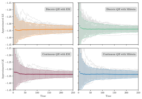
Figure 1: Discrete and continuous $QR$-based approximations of the LE corresponding to SDAE (29) via Euler-Maruyama and Milstein integrators, with a stepsize $h={1}\mathrm{e}{-3}$ and $T=250$. The solid circles show mean and the whiskers the $95\%$ confidence intervals of the trajectories.

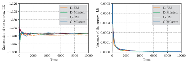
Figure 2: Discrete and continuous $QR$-based approximations of the LE corresponding to SDAE (29) via Euler-Maruyama and Milstein integrators, with a stepsize $h={1}\mathrm{e}{-3}$ and $T=10000$. The black dashed line in the left-hand side subplot shows the analytic value of $\lambda$.

A large number of simulations have been carried out for stepsizes $h={1}\mathrm{e}{-2},\,{9}\mathrm{e}{-3},\ldots,\,{1}\mathrm{e}{-3}$ with $T=1000,\,2000,\ldots,\,12000$; to obtain computed approximations of the LE truncated at the final time $t_{f}:=T$, denoted by $\lambda_{T}$. To complete our stochastic numerical analysis of the LE, we have calculated the values of expectation $\mathbb{E}[\lambda_{T}]$, standard deviation $\sigma[\lambda_{T}]$, and variance $\mathbb{V}[\lambda_{T}]$; estimated from $100$ independent realizations. Some results are presented in Tables (Appendices) to (Appendices), taking $T=6000,12000,20000$ and $h={1}\mathrm{e}{-1},\,{1}\mathrm{e}{-2},\,{1}\mathrm{e}{-3}$.

Observe that the time scale in Figure 1 has been conveniently adjusted to the range $[0,\,250]$, in order to show the exponential drop of the LE for the different realizations in the four methods, along the time evolution. While in Figure 2 the time scale has been adjusted to the range $[0,\,10000]$, to better display the convergence of the mean and variance of the LE.

Based on the analytic expression of the LE, given by equation (31), the LE $\lambda$ can be considered as a deterministic quantity. According to the numerical results obtained from the four $QR$-based methods, the sequences of random variables $\lambda_{t_{\ell}}$ reveal a trend towards null variance and convergence to the mean as $\ell$ tends to infinity. Such evolution can be seen in Figure 1, and more obviously in Figure 2. For all the methods, an exponential decay is illustrated in $\mathbb{E}[\lambda_{t_{\ell}}]$ and $\mathbb{V}[\lambda_{t_{\ell}}]$ as $\ell$ tends to infinite. This behavior indicates a mean square (m.s.) convergence of those sequences to a degenerate random variable, based on the implication that if $\lambda_{t_{\ell}}$ is such that $\mathbb{E}[\lambda_{t_{\ell}}]=\mu_{\lambda}$, for all $\ell$, and $\mathbb{V}[\lambda_{t_{\ell}}]\xrightarrow[\ell\rightarrow\infty]{}0$, then $\lambda_{t_{\ell}}\xrightarrow[\ell\rightarrow\infty]{\textrm{m.s.}}\mu_{\lambda}$. This means that the limit of $\lambda_{t_{\ell}}$ can be interpreted as a deterministic value with probability $1$. This enables us to state that the stochastic approximations $\lambda_{t_{\ell}}$ converge in m.s. sense to a number (a degenerate random variable), which is expected to represent the LE $\lambda$.

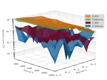
Figure 3: Comparison of relative errors for discrete and continuous $QR$-based approximations of the LE corresponding to SDAE (29) via Euler-Maruyama and Milstein integrators, with a range of stepsizes between $h={1}\mathrm{e}{-2},\ldots,{1}\mathrm{e}{-3}$; and with $T=1000,\ldots,12000$.

In Figure 3 we compare the relative error of the accuracy of the four numerical methods for different stepsize $h$ and time interval $[0,T]$. From this graphical representation, we observe that continuous methods obtain better results than discrete ones, as expected. We also observe that the Milstein method has, in general, better accuracy than the Euler-Maruyma scheme, since its convergence order is higher, but requies more computational time. This latter fact is evidenced in Figure 4, where a comparison of CPU time (in seconds) is shown for different values of $h$ and $T$. Here, we observe that all the methods are affected to the same extent by incrementing the simulation interval $T$, via a logarithmic increment, and by narrowing the stepsizes $h$, via an exponential increment. A more pronounced difference between the methods should be observed in higher dimensional systems.

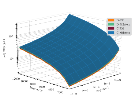
Figure 4: Comparison of the computing-time for discrete and continuous $QR$-based approximations of the LE corresponding to SDAE (29) via Euler-Maruyama and Milstein integrators, with a range of stepsizes between $h={1}\mathrm{e}{-2},\ldots,{1}\mathrm{e}{-3}$; and with $T=1000,\ldots,12000$.

4 Application of LEs to Power Systems Stability Analysis

The concept of stability (based on Lyapunov exponents) in power systems is, in essence, the same as that for a general dynamical system. In the literature, power system stability is defined as the stability to regain an equilibrium state after being subjected to physical disturbances [21, 22]. Such equilibrium is characterized through three significant quantities during the power system operation: angles of nodal voltages, frequency, and nodal voltage magnitudes. Based on this triplet, there is an entire classification proposed by the Institute of Electrical and Electronics Engineers (IEEE) and the International Council on Large Electric Systems (CIGRE) in [22], which is illustrated in Figure 5.

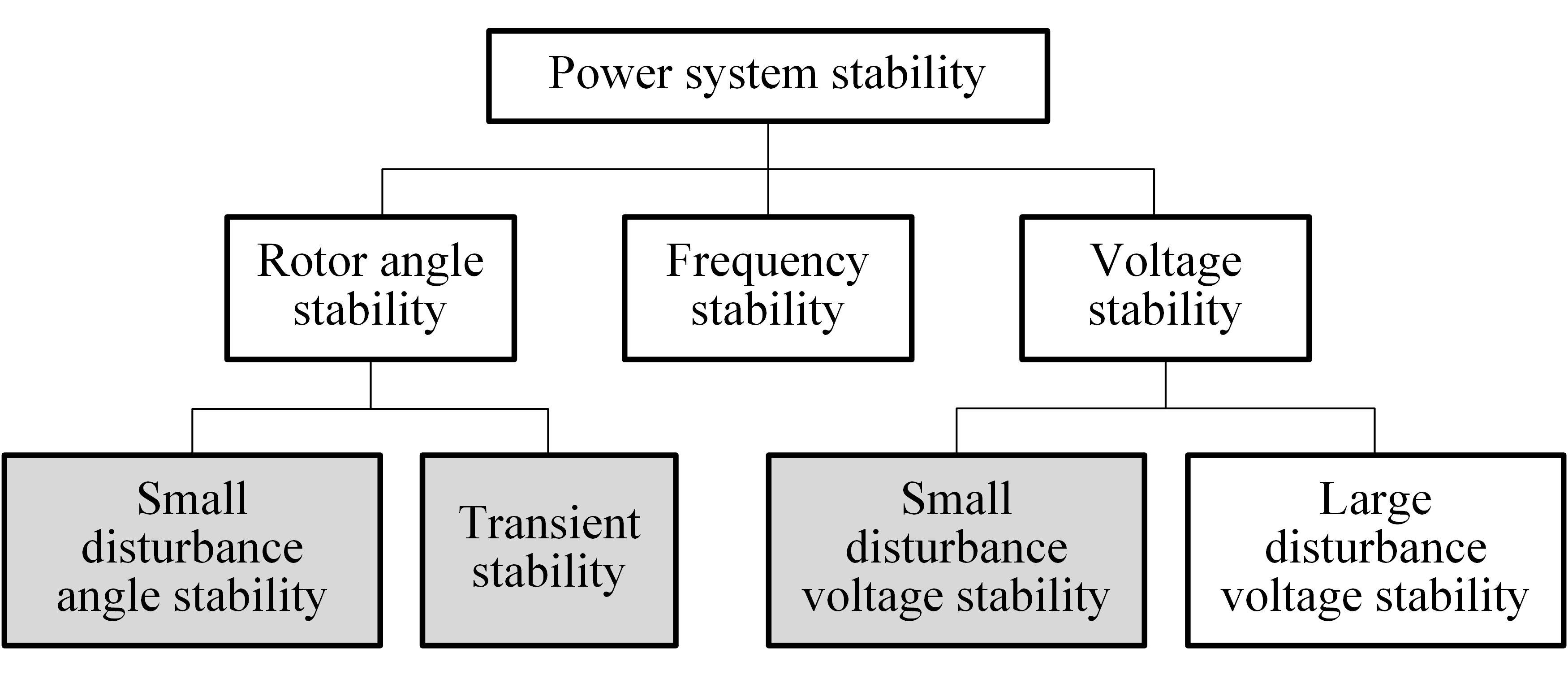
Figure 5: IEEE/CIGRE Power systems stability classification [22].

The test cases presented in this paper are oriented to evaluate the angle and voltage stability of power systems subjected to small or large disturbances. Studies considering small disturbances are commonly known as small-signal stability assessment (SSSA). Here, linear stability analysis via eigenvalues has been one of the traditional analysis tools to predict the degree of stability of the power system [21, 36]. However, eigenvalue analysis is limited to linear time-invariant systems or systems close to a stationary solution. When time-varying systems are tested, as is the case of systems subjected to stochastic disturbances, then eigenvalue analysis is no longer applicable. On the other hand, the stability analysis of power systems affected by large disturbances, known as transient stability assessment, is mainly performed with verification strategies based on time-domain integration [22, 29].

Since the concept of LEs is based on the trajectories of the dynamical systems, the method is an interesting measure of dynamic stability for power systems under stochastic disturbances in general. So, testing asymptotic stability of power systems via LEs has become an attractive approach for the two areas mentioned before, namely, the SSSA of rotor angles and voltages, by using the linearized set of SDAEs which model the system [40, 39]; and strategies for the rotor angles via transient analysis using the nonlinear SDAE system and its variational equation [19], [41]. For both cases, asymptotic stability is checked via approximations of the largest Lyapunov exponent (LLE) of the system. In particular, a negative LLE indicates that the dynamics of the system is asymptotically stable. In the next subsections test cases are presented that illustrate for strangenss-free SDAE systems the negativity of the LLE.

4.1 Modeling Power Systems through SDAEs

Under the assumption of deterministic dynamic behavior, power systems are typically modelled via a system of quasi-linear DAEs with partitioned variables, see [21],[36], of the form

$$\boldsymbol{E}_{11}d\boldsymbol{x}_{t}^{D_{1}} =\boldsymbol{f}_{0}^{D_{1}}(\boldsymbol{x}_{t}^{D_{1}},\boldsymbol{x}_{t}^{A})dt,$$ (32a)

$$0 =\boldsymbol{f}_{0}^{A}(\boldsymbol{x}_{t}^{D_{1}},\boldsymbol{x}_{t}^{A}),$$ (32b)

where $\boldsymbol{E}_{11}\in\mathbb{R}^{d_{1}\times d_{1}}$ is a diagonal block matrix, $\boldsymbol{f}_{0}^{D_{1}}\in\mathcal{C}^{1}(\mathbb{R}^{d_{1}+a},\mathbb{R}^{d_{1}})$, $\boldsymbol{f}_{0}^{A}\in\mathcal{C}^{1}(\mathbb{R}^{d_{1}+a},\mathbb{R}^{a})$, $\boldsymbol{x}_{t}^{D_{1}}\in\mathbb{R}^{d_{1}}$ are the dynamic state variables, and $\boldsymbol{x}_{t}^{A}\in\mathbb{R}^{a}$ are the algebraic state variables and we set $n_{1}=d_{1}+a$. The DAE system (32) is strangeness-free (of index one).

The dynamic behavior of synchronous machines, system controllers, power converters, transmission lines, or power loads are adequately represented through such a DAE formulation. But in current real world systems, the dynamic behavior of power systems is affected by disturbances of a stochastic nature such as renewable stochastic power generation, rotor vibrations in synchronous machines, stochastic variations of loads, electromagnetic transients, or perturbations originated by the measurement errors of control devices, see [31]. Such disturbances can be modeled through Itô SDEs of the form

$$d\boldsymbol{x}^{D_{2}}_{t}=\boldsymbol{f}_{0}^{D_{2}}(\boldsymbol{x}^{D_{1}}_{t},\boldsymbol{x}_{t}^{D_{2}},\boldsymbol{x}_{t}^{A})dt+\boldsymbol{f}_{1}^{D_{2}}(\boldsymbol{x}^{D_{1}}_{t},\boldsymbol{x}_{t}^{D_{2}},\boldsymbol{x}_{t}^{A})dw_{t}.$$ (33)

Here, $\boldsymbol{f}_{0}^{D_{2}}\in\mathcal{C}^{1}(\mathbb{R}^{d_{2}+a},\mathbb{R}^{d_{2}})$ is the drift, $\boldsymbol{f}_{1}^{D_{2}}\in\mathcal{C}^{2}(\mathbb{R}^{d_{2}+a},\mathbb{R}^{a})$ is the diffusion, $\boldsymbol{x}_{t}^{D_{2}}\in\mathbb{R}^{d_{2}}$ are the stochastic variables, and $w_{t}$ is the Wiener process. By combining (33) and (32), and assuming that $\boldsymbol{x}_{t}^{D_{2}}$ perturbs (32a) and (32b), we obtain a strangeness-free SDAE system of the form

$$\boldsymbol{E}_{1}d\boldsymbol{x}_{t}^{D_{1}} =\boldsymbol{f}_{0}^{D_{1}}(\boldsymbol{x}^{D_{1}}_{t},\boldsymbol{x}_{t}^{D_{2}},\boldsymbol{x}_{t}^{A})dt,$$ (34a)

$$d\boldsymbol{x}^{D_{2}}_{t} =\boldsymbol{f}_{0}^{D_{2}}(\boldsymbol{x}^{D_{1}}_{t},\boldsymbol{x}_{t}^{D_{2}},\boldsymbol{x}_{t}^{A})dt+\boldsymbol{f}_{1}^{D_{2}}(\boldsymbol{x}^{D_{1}}_{t},\boldsymbol{x}_{t}^{D_{2}},\boldsymbol{x}_{t}^{A})dw_{t},$$ (34b)

$$0 =\boldsymbol{f}_{0}^{A}(\boldsymbol{x}^{D_{1}}_{t},\boldsymbol{x}_{t}^{D_{2}},\boldsymbol{x}_{t}^{A}),$$ (34c)

or in simplified notation as

$$\boldsymbol{E}d\boldsymbol{x}_{t}=\boldsymbol{f}_{0}(\boldsymbol{x}_{t})dt+\boldsymbol{f}_{1}(\boldsymbol{x}_{t})dw_{t},\quad\boldsymbol{x}_{t_{0}}=\boldsymbol{x}_{0},$$ (35)

with

$$\boldsymbol{E}:=\left[\begin{smallmatrix}\boldsymbol{E}_{11}&0&0\\ 0&\boldsymbol{I}_{d_{2}}&0\\ 0&0&0\end{smallmatrix}\right],\ \boldsymbol{x}_{t}:=\left[\begin{array}[]{c}\boldsymbol{x}_{t}^{D_{1}}\\ \boldsymbol{x}^{D_{2}}_{t}\\ \boldsymbol{x}_{t}^{A}\end{array}\right],$$

drift $\boldsymbol{f}_{0}\in\mathcal{C}^{1}(\mathbb{R}^{n},\mathbb{R}^{n})$, and diffusion $\boldsymbol{f}_{1}\in\mathcal{C}^{2}(\mathbb{R}^{n},\mathbb{R}^{n})$, where $n=d_{1}+d_{2}+a$.

The study-cases presented below are formulated as the form (34). An alternative approach for including the stochastic disturbances is to implement the Wiener process directly in the underlying ODE of the system, turning them into SDEs (see [8, 16] for examples).

4.2 Modeling Stochastic Perturbations

In this subsection, we discuss on the modeling of stochastic variations via SDEs. We employ the well known mean-reverting process termed Ornstein–Uhlenbeck (OU) process [31, 17]. The SDE which defines the OU process has the form

$$d\eta_{t}=\alpha(\mu-\eta_{t})dt+\beta dw_{t},\qquad\eta_{t_{0}}=\eta_{0},\qquad t\in\mathbb{I},$$ (36)

where $\alpha,\mu,\beta\in\mathbb{R}^{+}$. The OU process is a stationary autocorrelated Gaussian diffusion process distributed as $\mathcal{N}(\mu,\beta^{2}/2\alpha)$. Another mean-reverting choice, similar to the OU process would be the Cox–Ingersoll–Ross (CIR) process, whose realizations are always nonnegative, in fact, it as a sum of squared OU process [1].

It is usually recommended to ensure the boundedness of the stochastic variations for the numerical implementations. In this regard, suitable resources are odd trigonometric functions such as a $\sin$ or $\arctan$ to guarantee boundedness. For example, if from (36) we generate a process with a normal distribution $\mathcal{N}(\mu,\sigma^{2})$, for $\mu=0$ and $\sigma^{2}=0.16$, this value of variance enables us to generate a mean-reverting stochastic trajectory, whose confidence interval of $95\%$ ($\pm 2\sigma$) is inside the threshold of $\pm 1$. Then, through the functions

$$\xi(\eta_{t})=\sin\eta_{t},\qquad\textrm{or}\qquad\chi(\eta_{t})=\frac{2}{\pi}\arctan\eta_{t},$$ (37)

we obtain a bounded stochastic variation inside the interval $[-1,1]$, and the OU SDEs, that generate the stochastic variations, are represented by (34b).

To couple the parameters of the system in (34a) and (34c) with a bounded stochastic disturbance, we use

$$p(\eta_{t})=p_{0}+\rho\xi(\eta_{t}),$$

where $p_{0}$ is a constant parameter, $\eta_{t}$ is the stochastic process that describes the variations of the parameter, and $\rho\in\mathbb{R}^{+}$ is a factor that controls the magnitude of the perturbation.

4.3 Test Cases

In this subsection we present results of our implementation of the $QR$-based methods for the calculation of LEs at the hand of several test cases of power systems represented by strangeness-free SDAEs models of so-called single-machine-infinite-bus (SMIB) systems. This simplified model is frequently used in the area of power systems in order to understand the local dynamic behavior of a specific machine connected to a complex power network. The SMIB consists of a synchronous generator connected through a transmission line to a bus with a fixed bus voltage magnitude and angle, called infinite bus, which represents the grid. A diagram of the system is shown in Figure 6.

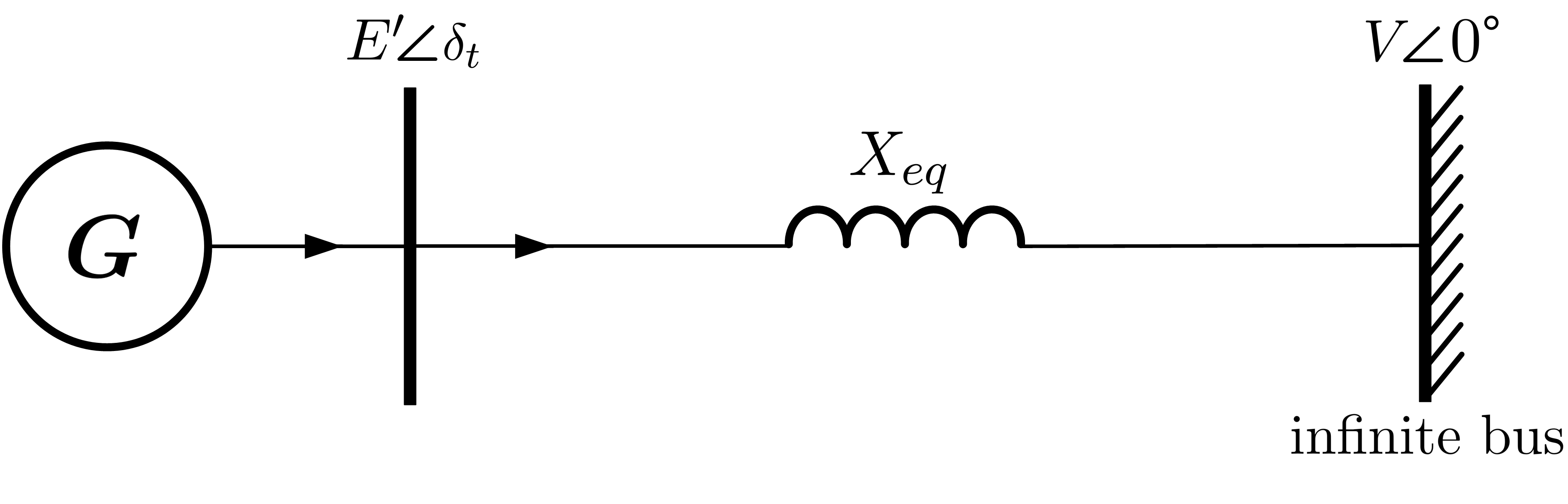
Figure 6: Single-machine infinite-bus (SMIB) scheme.

In each test case, we consider a different type of disturbance. For Case 1, the disturbance is a stochastic load connected to the system. In Case 2, the disturbance is due to noise caused by a measurement error in a transducer of the machine control system. In both cases, the maximum disturbance that the system can admit without loosing stability is analyzed, as well as the effect (positive or negative) of the disturbance for the system in the stable region. The whole SMIB system, i.e., the synchronous machine, system constraints, and stochastic disturbances; are modeled by a strangeness-free SDAE system. The dimension of this system is mainly defined by the type of model used in the synchronous machine; we use a classical model and a flux-decay model, see [21, 29, 35, 36] for detailed descriptions.

4.3.1 Case 1: SMIB with stochastic load

In this test case we make use of the LEs to assess the impact of stochastic disturbances associated with an active power load, over the rotor angle stability of a synchronous generator. Both the machine and load are connected to the same bus, and this bus in turn, is linked to the grid through a transmission line. This kind of SMIB model is typically used to analyze the effects of renewable energy sources, or aggregated random power consumption, see Figure 7.

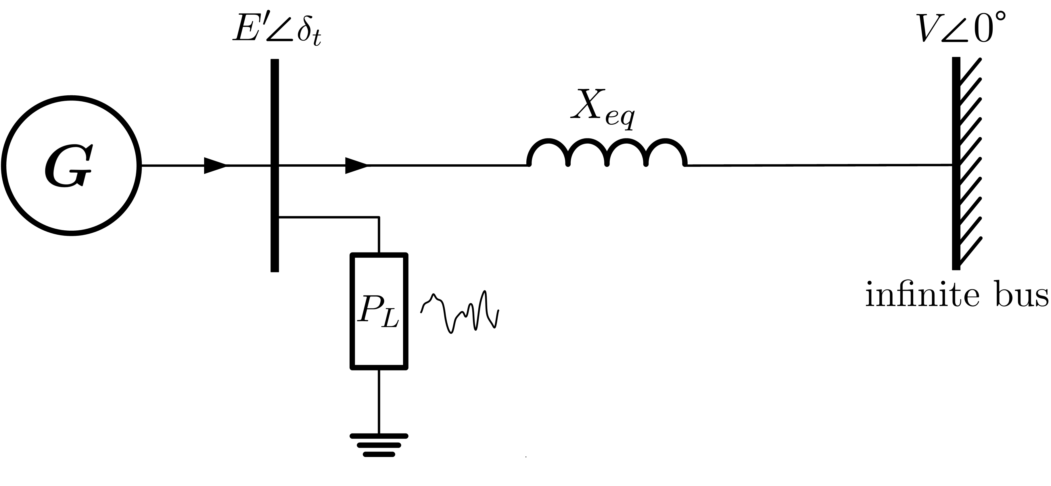
Figure 7: Scheme of a SMIB system with a stochastic load used in Test Case 1.

For this version of SMIB system called classical model, the dynamic behavior of the synchronous machine is represented by the swing equations where the rotor angle $\delta_{t}$ and the rotor speed $\omega_{t}$ are the state variables, see [29, 36]. The algebraic constraint in the system is given by the active power balance, expressed in terms of $P_{m}$ the mechanical power, $P_{e}$ the electrical power, and $P_{L}$ the constant power consumed by the load. A stochastic process $\eta_{t}$ is modeled by an OU SDE. We consider that $\rho\eta_{t}$ is the stochastic component of power consumption that perturbs additively the active power balance of the system, where $\rho$ is the size of the disturbance. This leads to the system

$$d\delta_{t} =[\omega_{t}-\omega_{s}]dt,$$ (38a)

$$2Hd\omega_{t} =[P_{m}-P_{e}-K_{D}(\omega_{t}-\omega_{s})]dt,$$ (38b)

$$\eta_{t} =-\alpha\eta_{t}dt+\beta dw_{t},$$ (38c)

$$0 =\frac{E^{\prime}V}{X_{eq}}\cos\delta_{t}+(P_{L}+\rho\eta_{t})-P_{e}.$$ (38d)

By computing the LEs of this SDAE system and checking the LLE, we can determine the maximal perturbation size $\rho$ (via successive increments of $\rho$) admitted by the SMIB system before loosing rotor angle stability. The numerical tests are performed for the values $P_{m}=0.8$; $P_{L}=0.3$; $X_{eq}=0.8$; $H=3.5$; $K_{D}=0.4$; $\omega_{s}=2\pi 50$; $V=1.0$; $E^{\prime}=1.05$; $\alpha=1.0$; $\beta=0.4$. Most of the values are expressed in the per-unit system (pu) [35]. The $QR$ methods are executed with step size $h={1}\mathrm{e}{-3}$ and a simulation time $T=20000$.

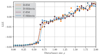
Figure 8: LLE considering different disturbance sizes $\rho$ for the SMIB Test Case 1, tested with four $QR$-based methods.

Figure 8 displays the computed LLE utilizing the four $QR$-based methods for incremental disturbance sizes $\rho=0.00,0.05,\ldots,2.00$. As expected, at $\rho=0.0$ when the system is not affected by a stochastic disturbance, i.e., the system is deterministic, the computed LEs match closely with the real parts of the eigenvalues obtained from the Jacobian matrix of the linearization of (38). When increasing $\rho$, all methods reveal the same monotonically increasing behavior of the calculated value of the LLE towards the unstable region. First, there is a slow increase for $0.00<\rho<0.60$, and then an abrupt increase of the LLE in the interval $0.60<\rho<0.75$. In the interval $0.75<\rho<1.20$, even though the LLE has not yet reached the instability region, for this particular case the characteristics such as a low damping coefficient and the presence of the stochastic disturbance, provokes a behavior in the system called pole slipping. This is, in a certain sense, a different kind of instability because the system looses synchronism as it reaches another equilibrium point near another attractor, see [36, sec. 5.8] for further details. The numerical results for this case are presented in Table Appendices.

This test case shows the large potential of using LEs as an indicator of instability for nonlinear power systems. These could be used also in multi-machine study cases where, however, the computational complexity has to be reduced, e.g. by model reduction.

4.3.2 Case 2: SMIB with regulator perturbed by noise

In this subsection we consider an SMIB system with a synchronous machine described by a third-order flux-decay model. Here, in addition to the rotor angle $\delta_{t}$ and the rotor speed $\omega_{t}$ associated to the swing equations, the system includes the effect of the field flux $\psi_{fd}$ described by the field circuit dynamic equations and constraints. In this model the machine is equipped with an automatic voltage regulator (AVR) to keep the generator output voltage magnitude in a desirable range, and a power system stabilizer (PSS) to damp out low-frequency oscillations, see Figure 9.

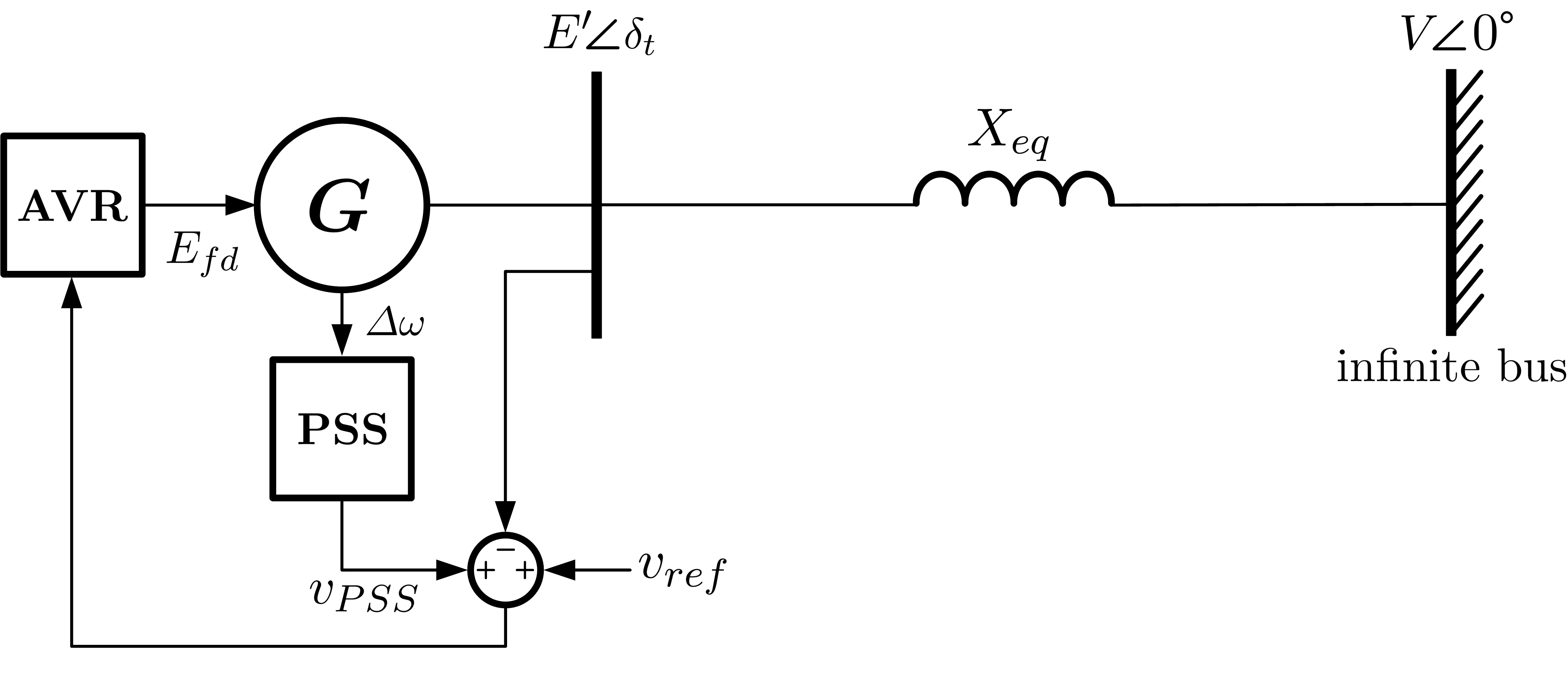
Figure 9: SMIB system scheme equipped with AVR and PSS, corresponding to Test Case 2.

The AVR and PSS add to the system three more state variables $v_{1}$, $v_{2}$, and $v_{s}$; together with their corresponding DAEs, which describe the dynamic behavior and constraints of the controllers into the SMIB system. The resulting model is a nonlinear system of strangeness-free DAEs. We use the LEs to analyze the system stability at a specific operation point in the state-space when it is subjected to small-disturbances. Using the small-signal stability assessment (SSSA), the set of DAEs that describes the dynamics of the power system is linearized around the desired operating point. The final result is a linear DAE system. A comprehensive explanation of this model, its linearization, and reduction to an underlying ODE system can be found in [21, ch. 12]. We consider a disturbance of stochastic nature entering in the exciter block of the AVR as an error of the reference signal [21, 40], by adding the stochastic variable $\eta$ to $v_{1}$ in equation (39c). Resolving the algebraic constraints leads to the linearized system of SDEs

$$d\Delta\delta =\omega_{s}\Delta\omega dt,$$ (39a)

$$2Hd\Delta\omega =\left[-K_{1}\Delta\delta-K_{D}\Delta\omega-K_{2}\Delta\psi_{fd}+\Delta T_{m}\right]dt,$$ (39b)

$$T_{3}\Delta\psi_{fd} =\left[-K_{3}K_{4}\Delta\delta-(1+K_{3}K_{6}K_{A})\Delta\psi_{fd}-K_{3}K_{A}(1+\rho\eta)\Delta v_{1}\right.$$

$$\quad\left.+K_{3}K_{A}\Delta v_{s}\right]dt,$$ (39c)

$$T_{R}d\Delta v_{1} =\left[-K_{5}\Delta\delta+K_{6}\Delta\psi_{fd}-\Delta v_{1}\right]dt,$$ (39d)

$$d\Delta v_{2} =\left[-K_{1}K_{ST}\Delta\delta-K_{D}K_{ST}\Delta\omega-K_{2}K_{ST}\Delta\psi_{fd}-\frac{1}{T_{W}}\Delta v_{2}+\frac{K_{ST}}{2H}\Delta T_{m}\right]dt,$$ (39e)

$$T_{2}d\Delta v_{s} =\left[-K_{1}K_{ST}T_{1}\Delta\delta-K_{D}K_{ST}T_{1}\Delta\omega-K_{2}K_{ST}T_{1}\Delta\psi_{fd}+\left(\frac{T_{1}}{T_{W}}+1\right)\Delta v_{2}\right.$$

$$\quad\left.-\frac{1}{T_{2}}\Delta v_{s}+\frac{K_{ST}T_{1}}{2H}\Delta T_{m}\right]dt,$$ (39f)

$$d\eta =-\alpha\eta dt+\beta dw,$$ (39g)

where $\Delta\delta,\ \Delta\omega,\ \Delta\psi_{fd},\ \Delta v_{1},\ \Delta v_{2},\ \Delta v_{s},\ \eta$ are the state variables of the linear underlying SDE system (for simplicity, the subscript $t$ has been omitted in this formulation). Once again, the stochastic perturbation is generated via an OU SDE, and the size of the perturbation is controlled by the parameter $\rho$. The numerical analysis is done for the values $\omega_{s}=2\pi 60$; $H=3.0$; $K_{1}=1.591$; $K_{2}=1.50$; $K_{D}=0.0$; $K_{3}=0.333$; $K_{4}=1.8$; $K_{5}=-0.12$; $K_{6}=0.3$; $K_{A}=200.0$; $T_{R}=0.02$; $K_{ST}=9.5$; $T_{1}=0.154$; $T_{2}=0.033$; $T_{3}=1.91$; $T_{W}=1.4$; $\alpha=1.0$; $\beta=0.4$; $\Delta T_{m}=0.0$.

Based on the analysis of Section (3.4), we only consider the continuous Euler-Maruyama QR method. The results of computing the LLE of the SMIB system for incremental values of the perturbation size $\rho$, are presented graphically in Figure 10.

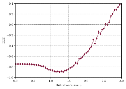
Figure 10: Computed LLE for the dimension 7 SMIB system of Test Case 2, considering different disturbance sizes and using the continuous Euler-Maruyama $QR$ method.

The values of the LLE when increasing perturbation size $\rho$ clearly mark four defined intervals. In the leftmost interval with $0.00<\rho<0.40$, the calculated LLE is practically constant and equal to the real part of the right-most eigenvalue from the deterministic system. In this region, there is no impact of the disturbance on the system stability. In the interval $0.40<\rho<1.30$ a curious situation occurs, as the size of the disturbance increases, the distance from the LLE to the positive region increases, in other words, the noise improves the stability of the system. In the interval $1.30<\rho<2.60$, the situation changes completely, and the LLE converges to zero. Finally, from $\rho\approx 2.60$ onwards, the system is unstable. Table Appendices shows the numerical values of this test case.

Finally, we have evaluated the computing-times for this 7-dimensional test case. The results are shown in Figure 11. Although the computational cost for all method is similar for the different methods as a factor of the step sizes $h$ and time interval $[0,T]$, the computational costs strongly increase.

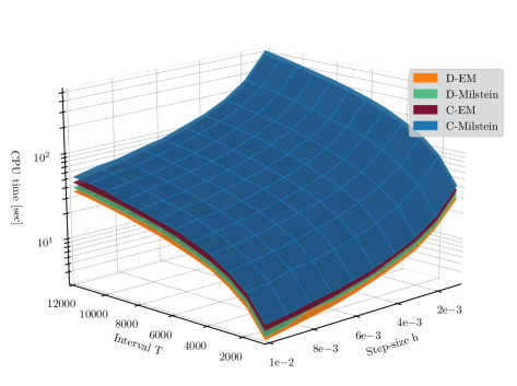
Figure 11: Computing-time comparison of LE calculation for the dimension 7 SMIB Test Case 2. Comparison performed for the four $QR$ methods in a range of step sizes between $h=[{1}\mathrm{e}{-2},{1}\mathrm{e}{-3}]$ and with $T=[1000,12000]$.

5 Conclusions

We have revisited the theory of strangeness-free SDAE systems, as well as the concepts of LEs associated with the RDEs generated via such SDAEs. We have adapted and implemented stochastic versions of continuous and discrete $QR$-based methods to calculate approximations of the LEs, and assessed them by using Euler-Maruyama and Milstein schemes over the corresponding underlying SDE. The results obtained from our numerical experiments illustrate the approximations of the corresponding LE converge to degenerate random variables, i.e., the LE can be interpreted as a deterministic value, since in the limit the variance of the approximations tends to zero. Both $QR$-based method provide reliable results, but in general, continuous methods provide better accuracy than the discrete counterpart at the expenses of higher computational cost and higher memory requirement. We have illustrated the $QR$-based methods for SMIB power system problems and shown the usefulness of the LEs as a stability indicator for the rotor angle and voltage stability analysis of power systems affected by bounded stochastic disturbances.

As future work, we suggest the use of discretization schemes for SDAEs in order to directly apply the numerical integration to the SDAE system. Furthermore, methods for computing the LEs based on Singular Value Decompositions, a combination with model reduction, and a careful comparison with QR-based methods would be of interest. Concerning to the applications to power systems and dynamical network systems in general, stability assessment of large-scale cases are remarkable works to be performed.

Appendices

In this Appendix we present the numerical values for several different simulations.

$T$	$h$	$\mathbb{E}[\lambda_{T}]$	$\sigma[\lambda_{T}]$	$\mathbb{V}[\lambda_{T}]$	Rel. error [%]	CPU-time [sec]
$6000$	${1}\mathrm{e}{-1}$	$-1.51906$	$0.00476$	${2.266}\mathrm{e}{-5}$	$13.48994$	$0.9827$
$6000$	${1}\mathrm{e}{-2}$	$-1.35231$	$0.00296$	${8.734}\mathrm{e}{-6}$	$1.03179$	$12.6422$
$6000$	${1}\mathrm{e}{-3}$	$-1.33874$	$0.00234$	${5.483}\mathrm{e}{-6}$	$0.01807$	$125.6875$
$12000$	${1}\mathrm{e}{-1}$	$-1.51870$	$0.00334$	${1.116}\mathrm{e}{-5}$	$13.46268$	$2.0336$
$12000$	${1}\mathrm{e}{-2}$	$-1.35217$	$0.00184$	${3.392}\mathrm{e}{-6}$	$1.02160$	$24.9517$
$12000$	${1}\mathrm{e}{-3}$	$-1.33920$	$0.00161$	${2.579}\mathrm{e}{-6}$	$0.05206$	$252.4366$
$20000$	${1}\mathrm{e}{-1}$	$-1.51780$	$0.00262$	${6.858}\mathrm{e}{-6}$	$13.39551$	$3.3806$
$20000$	${1}\mathrm{e}{-2}$	$-1.35236$	$0.00139$	${1.944}\mathrm{e}{-6}$	$1.03533$	$41.2975$
$20000$	${1}\mathrm{e}{-3}$	$-1.33936$	$0.00133$	${1.781}\mathrm{e}{-6}$	$0.06437$	$416.3228$

Table A.1: Numerical results of the calculated LE for SDAE system (29) computed via Discrete $QR$-EM method.

Table A.2: Numerical results of the calculated LE for SDAE system (29) computed via Discrete $QR$-Milstein method.

Table A.3: Numerical results of the calculated LE for SDAE system (29) computed via Continuous $QR$-EM method.

Table A.4: Numerical results of the calculated LE for SDAE system (29) computed via Continuous $QR$-Milstein method.

Table A.5: Numerical results of the approximated LLE of SMIB system (38) corresponding to the study-case 1, computed via the four $QR$-based techniques.

Table A.6: Numerical results of the approximated LLE of SMIB system (39) corresponding to the study-case 2, computed via C-EM method.

References

- [1] E. Allen. Modeling with Itô Stochastic Differential Equations. Mathematical Modelling: Theory and Applications. Springer Netherlands, 2007.
- [2] L. Arnold. Lyapunov exponents of nonlinear stochastic systems. In F. Ziegler and G. I. Schuëller, editors, Nonlinear Stochastic Dynamic Engineering Systems, pages 181–201, Berlin, Heidelberg, 1988. Springer Berlin Heidelberg.
- [3] L. Arnold. Random Dynamical Systems. Monographs in Mathematics. Springer-Verlag, 1998,2003.
- [4] G. Benettin, L. Galgani, A. Giorgilli, and J.-M. Strelcyn. Lyapunov characteristic exponents for smooth dynamical systems and for hamiltonian systems; a method for computing all of them. part 1: Theory. Meccanica, 15(1):9–20, Mar 1980.
- [5] G. Benettin, L. Galgani, A. Giorgilli, and J.-M. Strelcyn. Lyapunov characteristic exponents for smooth dynamical systems and for hamiltonian systems; a method for computing all of them. part 2: Numerical application. Meccanica, 15(1):21–30, Mar 1980.
- [6] L. Biegler, S. Campbell, and V. Mehrmann. Control and Optimization with Differential-Algebraic Constraints. Advances in Design and Control. Society for Industrial and Applied Mathematics, 2012.
- [7] K. Brenan, S. Campbell, and L. Petzold. Numerical Solution of Initial-Value Problems in Differential-Algebraic Equations. Classics in Applied Mathematics. Society for Industrial and Applied Mathematics, 1996.
- [8] T. Caraballo and X. Han. Applied Nonautonomous and Random Dynamical Systems: Applied Dynamical Systems. Springer Briefs in Mathematics. Springer International Publishing, 2017.
- [9] F. Carbonell, R. Biscay, and J. C. Jimenez. QR-based methods for computing Lyapunov exponents of stochastic differential equations. International Journal of Numerical Analysis Modeling Series B, 1(2):147–171, 2010.
- [10] N. D. Cong and N. T. The. Stochastic differential-algebraic equations of index 1. Vietnam Journal of Mathematics, 38(1):117–131, 2010.
- [11] N. D. Cong and N. T. The. Lyapunov spectrum of nonautonomous linear stochastic differential algebraic equations of index-1. Stochastics and Dynamics, 12(4):1–16, 2012.
- [12] L. Dieci, R. Russell, and E. Van Vleck. On the computation of Lyapunov exponents for continuous dynamical systems. SIAM Journal on Numerical Analysis, 34(1):402–423, 1997.
- [13] L. Dieci, R. D. Russell, and E. S. V. Vleck. Unitary integrators and applications to continuous orthonormalization techniques. SIAM Journal on Numerical Analysis, 31(1):261–281, 1994.
- [14] L. Dieci and E. S. Van Vleck. Lyapunov and Sacker–Sell spectral intervals. Journal of Dynamics and Differential Equations, 19(2):265–293, 2007.
- [15] L. Dieci and E. S. V. Vleck. Lyapunov spectral intervals: Theory and computation. SIAM Journal on Numerical Analysis, 40(2):516–542, 2003.
- [16] B. J. Geurts, D. D. Holm, and E. Luesink. Lyapunov exponents of two stochastic Lorenz 63 systems. Journal of Statistical Physics, Dic 2019.
- [17] A. González-Zumba. Wind power grid integration: A brief study about the current scenario and stochastic dynamic modeling. Master’s thesis, Universitat Politècnica de València, 2017.
- [18] A. Grorud and D. Talay. Approximation of Lyapunov exponents of stochastic differential systems on compact manifolds. In A. Bensoussan and J. L. Lions, editors, Analysis and Optimization of Systems, pages 704–713, Berlin, Heidelberg, 1990. Springer Berlin Heidelberg.
- [19] B. Hayes and F. Milano. Viable computation of the largest Lyapunov characteristic exponent for power systems. In 2018 IEEE PES Innovative Smart Grid Technologies Conference Europe (ISGT-Europe), pages 1–6, 2018.
- [20] P. Kloeden and E. Platen. Numerical Solution of Stochastic Differential Equations. Stochastic Modelling and Applied Probability. Springer Berlin Heidelberg, 2010.
- [21] P. Kundur. Power System Stability and Control. McGraw–Hill, Palo Alto, California, United States, first edition edition, 1994.
- [22] P. Kundur, J. Paserba, V. Ajjarapu, G. Andersson, A. Bose, C. Cañizares, N. Hatziargyriou, D. Hill, A. Stankovic, C. Taylor, T. Van Cutsem, and V. Vittal. Definition and classification of power system stability ieee/cigre joint task force on stability terms and definitions. IEEE Transactions on Power Systems, 19(3):1387–1401, Aug 2004.
- [23] P. Kunkel and V. Mehrmann. Differential-Algebraic Equations: Analysis and Numerical Solution. EMS Textbooks in Mathematics. European Mathematical Society, 2006.
- [24] D. Küpper, A. Kværnø, and A. Rößler. A Runge-Kutta method for index 1 stochastic differential-algebraic equations with scalar noise. BIT Numerical Mathematics, 52(2):437–455, Jun 2012.
- [25] R. Lamour, R. März, and C. Tischendorf. Differential-Algebraic Equations: A Projector Based Analysis. Differential-Algebraic Equations Forum. Springer Berlin Heidelberg, 2013.
- [26] V. H. Linh and V. Mehrmann. Lyapunov, Bohl and Sacker-Sell spectral intervals for differential-algebraic equations. Journal of Dynamics and Differential Equations, 21(1):153–194, 2009.
- [27] V. H. Linh, V. Mehrmann, and E. S. Van Vleck. QR methods and error analysis for computing Lyapunov and Sacker-Sell spectral intervals for linear differential-algebraic equations. Advances in Computational Mathematics, 35(2):281–322, 2011.
- [28] A. Lyapunov. General Problem of the Stability Of Motion. Control Theory and Applications Series. Taylor & Francis, 1992.
- [29] J. Machowski, J. Bialek, and J. Bumby. Power System Dynamics: Stability and Control. Wiley, 2011.
- [30] X. Mao. Stochastic Differential Equations and Applications. Elsevier Science, 2007.
- [31] F. Milano and R. Zarate-Minano. A systematic method to model power systems as stochastic differential algebraic equations. Power Systems, IEEE Transactions on, 28(4):4537–4544, Nov 2013.
- [32] B. Oksendal. Stochastic Differential Equations: An Introduction with Applications. Universitext. Springer Berlin Heidelberg, 2013.
- [33] V. I. Oseledec. A multiplicative ergodic theorem. Ljapunov characteristic number for dynamical systems. Trans. Moscow Math. Soc., 19:197–231, 1968.
- [34] A. Pikovsky and A. Politi. Lyapunov Exponents: A Tool to Explore Complex Dynamics. Cambridge University Press, 2016.
- [35] H. R. Pota. The Essentials of Power System Dynamics and Control. Springer Singapore, first edition edition, 2018.
- [36] P. Sauer, M. Pai, and J. Chow. Power System Dynamics and Stability: With Synchrophasor Measurement and Power System Toolbox. Wiley-IEEE. Wiley, 2017.
- [37] O. Schein and G. Denk. Numerical solution of stochastic differential-algebraic equations with applications to transient noise simulation of microelectronic circuits. Journal of Computational and Applied Mathematics, 100(1):77–92, 1998.
- [38] D. Talay. Second-order discretization schemes of stochastic differential systems for the computation of the invariant law. Stochastics and Stochastic Reports, 29(1):13–36, 1990.
- [39] H. Verdejo, W. Escudero, W. Kliemann, A. Awerkin, C. Becker, and L. Vargas. Impact of wind power generation on a large scale power system using stochastic linear stability. Applied Mathematical Modelling, 40(17):7977–7987, 2016.
- [40] H. Verdejo, L. Vargas, and W. Kliemann. Stability of linear stochastic systems via Lyapunov exponents and applications to power systems. Applied Mathematics and Computation, 218(22):11021–11032, 2012.
- [41] D. P. Wadduwage, C. Q. Wu, and U. Annakkage. Power system transient stability analysis via the concept of Lyapunov exponents. Electric Power Systems Research, 104:183–192, 2013.
- [42] R. Winkler. Stochastic differential algebraic equations of index 1 and applications in circuit simulation. Journal of Computational and Applied Mathematics, 163(2):435–463, 2003.