NCTS-TH/2007

Weyl Anomaly induced Fermi Condensation and Holography

Chong-Sun Chu ^2,3 , Rong-Xin Miao ¹

¹School of Physics and Astronomy, Sun Yat-Sen University, 2 Daxue Road, Zhuhai 519082, China

²Physics Division, National Center for Theoretical Sciences, National Tsing-Hua University, Hsinchu 30013, Taiwan

³Department of Physics, National Tsing-Hua University, Hsinchu 30013, Taiwan

Abstract

Recently it is found that, due to Weyl anomaly, a background scalar field induces a non-trivial Fermi condensation for theories with Yukawa couplings. For simplicity, the paper consider only scalar type Yukawa coupling and, in the BCFT case, only for a specific boundary condition. In these cases, the Weyl anomaly takes on a simple special form. In this paper, we generalize the results to more general situations. First, we obtain general expressions of Weyl anomaly due to a background scalar and pseudo scalar field in general 4d BCFTs. Then, we derive the general form of Fermi condensation from the Weyl anomaly. It is remarkable that, in general, Fermi condensation is non-zero even if there was not a non-vanishing scalar field background. Finally, we verify our results with free BCFT with Yukawa coupling to scalar and pseudo-scalar background potential with general chiral bag boundary condition and with holographic BCFT. In particular, we obtain the shape and curvature dependence of the Fermi condensate from the holographic one point function.

1 Introduction

Similar to Bose Einstein condensation, Fermi condensation is an interesting quantum phenomena, which has wide a range of applications. The famous examples include the Cooper pair in BCS theory of superconductivity, which is the bound state of a pair of electrons in a metal with opposite spins. The chiral condensate of massless fermions is another example of Fermi condensation. In QCD the chiral condensate is an order parameter of transitions between different phases of quark matter in the massless limit. The condensation of fermionic atoms has been observed in experiment [1].

Recently, it is found that Weyl anomaly can induce Fermi condensation for theories with Yukawa couplings [2], when a background scalar is turned on. The mechanism is similar to the those of Weyl anomaly induced Casimir effect [5] and current [6, 7, 8]. For simplicity, [2] discusses only the free Dirac fermion theory with the action

$$I=\int_{M}\sqrt{|g|}\left(\bar{\psi}i\gamma^{i}\nabla_{i}\psi+\phi\bar{\psi}\psi\right),$$ (1)

where $\bar{\psi}=\psi^{\dagger}\gamma^{0}$ and $\phi$ is a background scalar field. We take signature $(1,-1,-1,-1)$ in this paper. The gamma matrix obeys

$$\{\gamma^{i},\gamma^{j}\}=2\ g^{ij}.$$ (2)

Imposing the following bag boundary condition (BC) [9, 10, 11]

$$(1\pm\gamma_{5}\gamma^{i}n_{i})\psi|_{\partial M}=0$$ (3)

and applying the heat kernel expansion [11], [2] gets Weyl anomaly at one loop

$$\mathcal{A}=\frac{1}{8\pi^{2}}\left(\int_{M}\sqrt{|g|}\Big{[}-(\nabla\phi)^{2}+\frac{R\phi^{2}}{6}+\phi^{4}\Big{]}+\int_{\partial M}\sqrt{|h|}\frac{k\phi^{2}}{3}\right).$$ (4)

Here $k=\nabla_{i}n^{i}$ and $n^{i}$ is the outward-pointing normal vector. From the action (1), it is clear that the Fermi condensation is given by the renormalization expectation value of the scalar operator ${\cal O}:=\bar{\psi}\psi$,

$$\langle\bar{\psi}\psi\rangle=\frac{1}{\sqrt{|g|}}\frac{\delta I_{\rm eff}}{\delta\phi},$$ (5)

where $I_{\rm eff}$ is the effective action of fermions. For a flat half space $x\geq 0$, it is remarkable that the Fermi condensation (5) can be derived from Weyl anomaly (4) as [2]

$$\langle\bar{\psi}\psi\rangle=-\frac{1}{4\pi^{2}}\frac{n^{i}\nabla_{i}\phi+\frac{1}{3}k\phi}{x}+O(\ln x),\quad x\sim 0,$$ (6)

where we have used $n^{i}\nabla_{i}\phi=-\partial_{x}\phi$ since $n^{i}=(0,-1,0,0)$.

In this paper, we generalize the work of [2] to more general class of boundary conditions in four dimensional CFT/BCFT [13, 14]. We show that, by imposing the Wess-Zumino consistency condition, one can obtain the general expression of Weyl anomaly due to a background scalar field (or pseudoscalar field) $\phi$ . Compared with (4), generally more boundary terms are allowed to appear. This is one of the main results of this paper. We then show that the presence of the Weyl anomaly implies that the scalar operator defined by

$${\cal O}:=\frac{1}{\sqrt{|g|}}\frac{\delta I}{\delta\phi}$$ (7)

obtains a nontrivial expectation value near the boundary. Generally new contributions that are independent of the background scalar field can arise. We show that this also occur in conformally flat spacetime without boundaries. This is another interesting result of this paper. Finally, we verify our results with the Yukawa theory of fermions coupled to a background scalar or pseudoscalar field with general BCs. We do the same for the holographic BCFT and we obtain, in particular, the shape and curvature dependence of the one point function of the dual scalar operator in strongly coupled CFT. This is an interesting quantity and we expect it to have non-trivial implications on the phase structure of the theory.

The paper is organized as follows. In section 2, we obtain the general expressions of Weyl anomaly for 4d BCFTs with a general shape of boundary in a curved spacetime, and in the presence of a background scalar field. In section 3, we show that the Weyl anomaly induces a condensation for the corresponding scalar operator ${\cal O}$ in a BCFT near the boundary or in a CFT in a conformally flat spacetime without boundaries. In section 4, we consider the Yukawa theory with general BCs and verify the anomalous Fermi condensation near the boundary. In section 5, we study the holographic one point function near the boundary of BCFT and verify that it takes the expected form as derived in section 3. In section 6, we give a holographic proof of the Weyl anomaly induced one-point function in conformally flat spacetime without boundaries. Finally, we conclude in section 7.

Conventions. People in the fields of quantum field theory and gravity theory usually use different signature of the metric [3, 4]. For the convenience of the reader, we take signature $(1,-1,-1,-1)$ in section 1- section 4 for the field-theoretical discussions, while signature $(1,1,1,1)$ or $(-1,1,1,1)$ in section 5 and section 6 for the holographic study. In signature $(1,-1,-1,-1)$ [3], $R^{i}_{\ jkl}=\partial_{l}\Gamma^{i}_{jk}-\partial_{k}\Gamma^{i}_{jl}+\Gamma^{i}_{lm}\Gamma^{m}_{jk}-\Gamma^{i}_{km}\Gamma^{m}_{jl}$, $R_{ij}=R^{l}_{\ ilj}$, $R=g^{ij}R_{ij}$, $k_{ij}=h^{k}_{i}h^{l}_{j}\nabla_{k}n_{l}$, $k=h^{ij}k_{ij}=\nabla_{i}n^{i}$ where $n^{i}$ is the normal vector given by $n^{i}=-n_{i}=(0,-1,0,0)$ in a flat half space $x\geq 0$. While in signature $(1,1,1,1)$ and $(-1,1,1,1)$ [4], $R^{i}_{\ jkl}=\partial_{k}\Gamma^{i}_{jl}-\partial_{l}\Gamma^{i}_{jk}+\Gamma^{i}_{km}\Gamma^{m}_{jl}-\Gamma^{i}_{lm}\Gamma^{m}_{jk}$, $R_{ij}=R^{l}_{\ ilj}$, $R=g^{ij}R_{ij}$, $k_{ij}=h^{k}_{i}h^{l}_{j}\nabla_{k}n_{l}$, $k=h^{ij}k_{ij}$ where $n^{i}$ is the outward-pointing normal vector. Note that Fermi condensation $\langle\bar{\psi}\psi\rangle$, stress tensor $T_{ij}$, Ricci scalar $R$, normal vector $n^{i}$ and the trace of extrinsic curvature $k$ are the same, while $R^{i}_{\ jkl},R_{ij},k_{ij},g_{ij},n_{i}$ and, in particular, the Weyl anomaly $\langle T^{i}_{i}\rangle$, differ by a minus sign in different signatures. Note that $R$ and $k$ agree with those of [11] in both signatures.

2 Weyl Anomaly due to Scalar Background

Let $\phi$ be a scalar field or pseudo-scalar field with dimension one, which we will consider as a background. Similar to the background gravitational field and gauge field, it leads to Weyl anomaly [15]. For a CFT/BCFT, the Weyl anomaly should be Weyl invariant and obey the Wess-Zumino consistency condition [16]

$$[\delta_{\sigma_{1}},\delta_{\sigma_{2}}]\mathcal{A}=0.$$ (8)

Imposing the above conditions, we obtain the general expressions of Weyl anomaly due to a background field $\phi$:

$$\mathcal{A}=a_{1}\mathcal{A}_{1}+a_{2}\mathcal{A}_{2}+\sum_{n=1}^{4}b_{n}\mathcal{B}_{n},$$ (9)

where $\mathcal{A}_{n},\mathcal{B}_{m}$ are given by

$$\mathcal{A}_{1}=\int_{M}\sqrt{|g|}[-(\nabla\phi)^{2}+\frac{1}{6}R\phi^{2}]+\int_{\partial M}\sqrt{|h|}\frac{1}{3}k\phi^{2},$$ (10)

$$\mathcal{A}_{2}=\int_{M}\sqrt{|g|}\phi^{4},$$ (11)

$$\mathcal{B}_{1}=\int_{\partial M}\sqrt{|h|}\phi^{3},$$ (12)

$$\mathcal{B}_{2}=\int_{\partial M}\sqrt{|h|}[k\phi^{2}+3\phi n^{i}\nabla_{i}\phi],$$ (13)

$$\mathcal{B}_{3}=\int_{\partial M}\sqrt{|h|}[R\phi+6\Box\phi],$$ (14)

$$\mathcal{B}_{4}=\int_{\partial M}\sqrt{|h|}[{\text{Tr}}\bar{k}^{2}\phi]$$ (15)

and $a_{n},b_{m}$ are the corresponding bulk and boundary central charges. Here $g_{ij},R,\nabla_{i},\Box$ are metrics, Ricci scalar, covariant derivatives and D’Alembert operator defined in the bulk $M$, $h_{ab}$ is the induced metric on the boundary $\partial M$, $n^{i}$ is the outpointing normal vector given by $n^{i}=-n_{i}=(0,-1,0,0)$ in a flat half space, $k_{ab}=h_{a}^{\ i}h_{b}^{\ j}\nabla_{i}n_{j}$ is the extrinsic curvature and $\bar{k}_{ab}=k_{ab}-\frac{1}{3}kh_{ab}$ is its traceless part.

Some comments are in order. 1. The bulk central charges $a_{n}$ are independent of boundary conditions, while the boundary central charges $b_{m}$ depend on boundary conditions. 2. Second, as mentioned above, the Weyl anomaly (9) obeys the Wess-Zumino consistency (8). 3. We consider only integer powers of $\phi$ and ignore terms including $\phi^{1/2},\phi^{1/3},...$. If such terms are allowed, we could construct scalar-invariant terms such as

$$\int_{\partial M}\sqrt{|h|}[-(D\phi^{\frac{1}{2}})^{2}+\frac{1}{8}\mathcal{R}\phi],$$ (16)

where $D_{a},\mathcal{R}$ are covariant derivatives and Ricci scalar on the boundary $\partial M$, respectively. However, since $(D\phi^{\frac{1}{2}})^{2}=\frac{1}{4}(D\phi)^{2}/\phi$ is not well-defined on points with $\phi=0$ but $D\phi\neq 0$, we rule out such possible contributions to Weyl anomaly. 4. We focus on CFT/BCFT in this paper. For general QFT, non-scale-invariant terms are allowed in Weyl anomaly. 5. We can rewrite $\mathcal{B}_{3}$ into more convenient form for the purpose to derive Fermi condensation

$$\mathcal{B}_{3}=\int_{\partial M}\sqrt{|h|}[R\phi-6n^{i}n^{j}\nabla_{i}\nabla_{j}\phi-6kn^{i}\nabla_{i}\phi+6D^{a}D_{a}\phi],$$ (17)

where the total derivative term $D^{a}D_{a}\phi$ can be dropped since $\partial M$ is closed, i.e., $\partial(\partial M)=0$. In the next section, we shall show that $\mathcal{B}_{3}$ is related to the leading term of Fermi condensation near the boundary.

3 Anomalous Condensation

In this section, we show that in four dimensional spacetimes with and without boundaries, the operator ${\cal O}$ that couples to the scalar field $\phi$ obtains a non-trivial expectation value due to the Weyl anomaly (9). For simplicity, we focus on the case of CFT/BCFT below. For the theory of Dirac fermions with Yukawa coupling to a background scalar field $\phi$, ${\cal O}=\bar{\psi}\psi$ and the expectation value $\langle{\cal O}\rangle$ gives Fermi condensation.

3.1 Spacetime with Boundary

Let us first investigate the case with boundaries. Since the mass dimension of scalar operator $O$ is three, its expectation value takes the asymptotic form [17]

$$\langle{\cal O}\rangle=\frac{O_{0}}{x^{3}}+\frac{O_{1}}{x^{2}}+\frac{O_{2}}{x}+O(x^{0},\ln x)$$ (18)

near the boundary. Here $x$ is the proper distance from the boundary, $O_{n}$ have mass dimension $n$ and depend on only the background geometry and background scalar. Below we will derive exact expressions of $O_{n}$ from the Weyl anomaly.

One way to see that the coefficients $O_{n}$ are directly connected with the Weyl anomaly is by noticing that the one point function (18) can be understood as a well-defined distribution [18, 19] if the inverse powers of $x$ are accompanied by logarithmically divergent contact terms $\ln x\;\partial^{n}_{x}\delta(x)$. Such contract terms determine the scale variation of $\langle O\rangle$ and hence the coefficients $O_{n}$ of (18) are in fact determiend by the central charges of Weyl anomaly . From this point of view, it is clear that the coefficient $O_{0}$ is completely determined by an anomaly coefficient instead of other non-anomalous data.

In this paper, we use an alternative method to derive $O_{n}$ from the Weyl anomaly. Using the fact that the Weyl anomaly is related to the UV Logarithmic divergent term of the effective action, one can [5, 8] establish the relation

$$(\delta\mathcal{A})_{\partial M}=(\delta I_{\rm eff})_{\log\epsilon}=\left(\int_{M}\sqrt{|g|}(\frac{1}{2}\langle T_{ij}\rangle\delta g^{ij}+\langle J_{i}\rangle\delta A^{i}+\langle{\cal O}\rangle\delta\phi)\right)_{\log\epsilon}$$ (19)

which relates directly the variation of the Weyl anomaly with a corresponding one-point function. Here a regulator $x\geq\epsilon$ to the boundary has been introduced in the integral on the RHS of (19) and the symbol $(\;)_{\log\epsilon}$ denotes the coefficient of the $\log\epsilon$ term. The first equation of (19) is due to the definition of Weyl anomaly, and the second equation of (19) is just the definition of one point functions. For our purpose, we will turn on only the variation of scalar and focus on

$$(\delta_{\phi}\mathcal{A})_{\partial M}=\left(\int_{M}\sqrt{|g|}\langle{\cal O}\rangle\delta\phi\right)_{\log\epsilon}.$$ (20)

The variations $\delta g^{ij},\delta A^{i}$, $\delta\phi$ are independent. Previously the one-point functions $\langle T_{ij}\rangle,\langle J_{i}\rangle$ have been studied. In this paper we will consider the scalar variation $\delta\phi$ and derive the one-point function $\langle{\cal O}\rangle$ from the Weyl anomaly.

To proceed, let us consider the metric written in the Gauss normal coordinates

$$ds^{2}=-dx^{2}+\left(h_{ab}(y)-2xk_{ab}(y)+x^{2}q_{ab}(y)+O(x^{3})\right)dy^{a}dy^{b}$$ (21)

and expand the scalar near the boundary as

$$\phi(x,y)=\phi_{0}(y)+x\phi_{1}(y)+\frac{x^{2}}{2}\phi_{2}(y)+O(x^{3})$$ (22)

where $n^{i}=-n_{i}=(0,-1,0,0)$ and $\phi_{m}$ are independent variables. From (9), we get the LHS of (20)

$$\int_{\partial M}\sqrt{|h|}\left(-6b_{3}\delta\phi_{2}+\left(6b_{3}k-3b_{2}\phi_{0}\right)\delta\phi_{1}\right)$$ (23)

$$+ \int_{\partial M}\sqrt{|h|}\left(\frac{2}{3}a_{1}k\phi_{0}-2a_{1}\phi_{1}+2b_{2}k\phi_{0}+b_{3}R+b_{4}\text{Tr}\bar{k}^{2}+3b_{1}\phi_{0}^{2}-3b_{2}\phi_{1}\right)\delta\phi_{0}$$

Next, we substitute (18) into the RHS of (20), integrate over $x$ and select the logarithmic divergent term, we obtain

$$\int_{\partial M}\sqrt{|h|}\left(-\frac{O_{0}}{2}\delta\phi_{2}-\left(O_{1}-kO_{0}\right)\delta\phi_{1}\right)$$ (24)

$$+ \int_{\partial M}\sqrt{|h|}\left(-\frac{1}{2}O_{0}\left(k^{2}+q-2\text{Tr}k^{2}\right)+kO_{1}-O_{2}\right)\delta\phi_{0},$$

where we have used $\sqrt{|g|}=\sqrt{|h|}\left(1-kx+\frac{1}{2}\left(k^{2}+q-2\text{Tr}k^{2}\right)x^{2}+O(x^{3})\right)$ and $q=h^{ab}q_{ab}$ in the above calculations. Comparing (23) and (24), we can solve

$$O_{0}=12b_{3},\ O_{1}=3\left(2b_{3}k+b_{2}\phi_{0}\right),$$

$$O_{2}=-2a_{1}(\frac{1}{3}k\phi_{0}-\phi_{1})-3b_{1}\phi_{0}^{2}+b_{2}(k\phi_{0}+3\phi_{1})-b_{3}(6q+R-12\text{Tr}k^{2})-b_{4}\text{Tr}\bar{k}^{2}.\;\;\;\;$$ (25)

From (5), (18) and (3.1), we finally obtain one of our main results for the expectation value of the Fermi condensation near the boundary:

$$\langle\bar{\psi}\psi\rangle = \frac{12b_{3}}{x^{3}}+\frac{6b_{3}k+3b_{2}\phi}{x^{2}}$$ (26)

$$+ \frac{-2a_{1}(n^{i}\nabla_{i}+\frac{1}{3}k)\phi-3b_{1}\phi^{2}+b_{2}k\phi-b_{3}(R+6R_{nn}-6\text{Tr}k^{2})-b_{4}\text{Tr}\bar{k}^{2}}{x}$$

$$+ O(x^{0},\ln x),$$

where $\phi=\phi(x)=\phi_{0}+x\phi_{1}+\cdots$ in the above expression. Above we have rewritten $O_{n}$ into covariant expressions and have used $R_{nn}=q-\text{Tr}k^{2}$ in Gauss normal coordinates.

Let us make some comments. 1. (26) shows that the leading terms of Fermi condensation near the boundary are completely fixed by central charges of Weyl anomaly. In general, the boundary central charge depends on choices of boundary conditions, so does the Fermi condensation (26). 2. Similar to the case of current and stress tensor [8, 5], there are boundary contributions to the Fermi condensation, which can cancel the “bulk divergence” and make finite the total Fermi condensation. 3. (26) works for general 4d BCFTs. For non-BCFTs, there are corrections to Weyl anomaly and thus corresponding corrections to Fermi condensation (26) . 4. (26) agrees with the results of the free theory with $b_{i}=0$ [2]

$$\langle\bar{\psi}\psi\rangle=\frac{-2a_{1}(n^{i}\nabla_{i}+\frac{1}{3}k)\phi}{x}+O(x^{0},\ln x)$$ (27)

Note that $\nabla_{n}$ of [2] denotes $\nabla_{x}$, so it is given by $-n^{i}\nabla_{i}$ in this paper. 5. In general in a curved spacetime and for curved boundary, the Fermi condensation (26) is non-vanishing even without a background scalar

$$\langle\bar{\psi}\psi\rangle_{\phi=0}=\frac{12b_{3}}{x^{3}}+\frac{6b_{3}k}{x^{2}}-\frac{b_{3}(R+6R_{nn}-6\text{Tr}k^{2})+b_{4}\text{Tr}\bar{k}^{2}}{x}+O(x^{0},\ln x).$$ (28)

This generalize the result of [2].

3.2 Conformally Flat Spacetime without Boundary

Let us next turn to discuss the case without boundaries. For simplicity, we focus on conformally flat spacetime. Let us start by deriving the anomalous transformation rule for the condensate. Consider a theory with metric and scalar field given by $(g_{ij},\phi)$. Due to the anomaly, the renormalized effective action $I_{\rm eff}$ is not invariant under the Weyl transformation. Consider the Weyl transformation

$$g_{ij}\to g_{ij}^{\prime}=e^{-2\sigma}g_{ij},\quad\phi\to\phi^{\prime}=e^{\sigma}\phi,$$ (29)

for arbitrary finite $\sigma(x)$, we have generally

$$\frac{\delta}{\delta\sigma}I_{\rm eff}(e^{-2\sigma}g_{ij},e^{\sigma}\phi)={\cal A}(e^{-2\sigma}g_{ij},e^{\sigma}\phi).$$ (30)

This can be integrated to give the effective action [16, 23, 24]. Using the fact that the anomaly (9) is Weyl invariant up to a surface term:

$${\cal A}(e^{-2\sigma}g_{ij},e^{\sigma}\phi)={\cal A}(g_{ij},\phi)+a_{1}\int_{M}\partial_{i}(\sqrt{-g}\phi^{2}g^{ij}\partial_{j}\sigma),$$ (31)

we obtain the transformation rule for the effective action:

$$I_{\rm eff}(e^{-2\sigma}g_{ij},e^{\sigma}\phi)=I_{\rm eff}(g_{ij},\phi)$$

$$+a_{1}\int_{M}\sqrt{|g|}\left[\left(-(\nabla\phi)^{2}+\frac{R\phi^{2}}{6}\right)\sigma+\frac{\phi^{2}}{2}(\nabla\sigma)^{2}\right]+\frac{a_{1}}{3}\int_{\partial M}\sqrt{|h|}k\phi^{2}\sigma$$

$$+a_{2}\int_{M}\sqrt{g}\phi^{4}\sigma+\sum_{n=1}^{4}b_{n}\mathcal{B}_{n}\sigma.$$ (32)

One can check that the effective action satisfies Wess-Zumino consistency $[\delta_{\sigma_{1}},\delta_{\sigma_{2}}]I_{\rm eff}=0$. This is a test of our results. Using (3.2), we obtain finally the anomalous transformation rule for the condensate (5) under Weyl transformation $g_{ij}\to g^{\prime}_{ij}=e^{-2\sigma}g_{ij}$, $\phi\to\phi^{\prime}=e^{\sigma}\phi$,

$$\langle O\rangle=-2a_{1}\nabla(\sigma\nabla\phi)-(\frac{a_{1}}{3}\phi R+4a_{2}\phi^{3})\sigma-a_{1}\phi(\nabla\sigma)^{2},$$ (33)

plus the term $e^{-3\sigma}\langle O\rangle^{\prime}$ and some boundary terms which we drop in spacetime without boundaries. Here $\langle O\rangle$ (resp. $\langle O\rangle^{\prime}$) denotes the vev of the condensate of the theory (88) in the background spacetime $g_{ij}$ (resp. $g^{\prime}_{ij}$). Taking $g^{\prime}_{ij}$ to be the flat spacetime metric and the fact that the Fermi condensation vanishes in flat spacetime, we finally obtain (33) as the Fermi condensate in conformally flat spacetime

$$ds^{2}=e^{2\sigma}\eta_{ij}dx^{i}dx^{j}.$$ (34)

For Dirac fermions with Yukawa coupling, we have $O=\bar{\psi}\psi$, $a_{1}=1/(8\pi^{2})$ and (33) reproduces the result of [2].

4 Yukawa Coupled Fermions

In this section, we investigate the anomalous Fermi condensation for the Yukawa coupled Dirac theory (1) with more general BCs. We will derive the general expression (9) for the Weyl anomaly and also the corresponding Fermi condensate.

The BCs of Dirac fields should make zero the normal current on the boundary. According to [14], the general BCs take the form

$$\Pi_{-}\psi|_{\partial M}=0,$$ (35)

where $\Pi_{\pm}=(1\pm\chi)/2$ are projection operators and $\chi$ satisfy [14]

$$\chi\gamma^{n}=-\gamma^{n}\bar{\chi},\ \chi\gamma^{a}=\gamma^{a}\bar{\chi},\ \chi^{2}=\bar{\chi}^{2}=1.$$ (36)

Here $\bar{\chi}=\gamma^{0}\chi^{+}\gamma^{0}$ and $n$ ($a$) denote the normal (tangent) directions. Without loss of generality, we choose

$$\chi=-ie^{i\theta\gamma_{5}}\gamma^{i}n_{i},$$ (37)

which defines the so-called chiral bag boundary condition

$$(1+ie^{i\theta\gamma_{5}}\gamma^{i}n_{i})\psi|_{\partial M}=0.$$ (38)

Here $\theta$ is a constant and $n_{i}$ is the normal vector given by $(0,1,0,0)$ in a flat half space. Note that the BC (38) reduces to the usual bag BC $(1\pm i\gamma^{i}n_{i})\psi|_{\partial M}=0$ for $\theta=0,\pi$. And it reduces to the BC (3) studied in [2] when $\theta=\pm\frac{\pi}{2}$.

From the BC (38) and EOM $(i\gamma^{i}\nabla_{i}+\phi)\psi=0$, one can derive that

$$\left(-n^{i}\nabla_{i}+S\right)\Pi_{+}\psi|_{\partial M}=0,$$ (39)

where

$$S=-(\phi\cos\theta+\frac{k}{2})\Pi_{+}$$ (40)

and

$$\Pi_{\pm}:=\frac{1}{2}(1\mp ie^{i\theta\gamma_{5}}\gamma^{i}n_{i}).$$ (41)

4.1 Fermi Condensate from Weyl Anomaly

In this subsection, we use heat-kernel method [11] to derive Weyl anomaly due to a background scalar. To apply the heat-kernel method, we need to construct a Laplace-type operator from the Dirac operator. Following [3], we define two operators

$$D=i\gamma^{i}\nabla_{i}+\phi,$$ (42)

$$\widetilde{D}=-i\gamma^{i}\nabla_{i}+\phi.$$ (43)

In even dimensions, $\{\gamma^{i}\}$ and $\{-\gamma^{i}\}$ form equivalent representations of Clifford algebra [3]. As a result, the effective action can be rewritten as

$$W=-i\ln\text{det}D=-\frac{i}{2}\ln\text{det}(\widetilde{D}D),$$ (44)

where

$$\widetilde{D}D=g^{ij}\nabla_{i}\nabla_{j}+\frac{1}{4}R+\phi^{2}-i\gamma^{i}\partial_{i}\phi:=g^{ij}\nabla_{i}\nabla_{j}-E,$$ (45)

where

$$E:=-\frac{1}{4}R-\phi^{2}+i\gamma^{i}\partial_{i}\phi.$$ (46)

Now we are ready to derive Weyl anomaly. Using the heat kernel coefficient in [11], the Weyl anomaly related to the background scalar is given by

$${\cal A} = \frac{1}{360(4\pi)^{2}}\int_{M}dx^{4}\sqrt{|g|}\Big{(}-60\Box E+60RE+180E^{2}\Big{)}$$ (47)

$$+ \frac{1}{360(4\pi)^{2}}\int_{M}dy^{3}\sqrt{|h|}\Big{(}-(240\Pi_{+}-120\Pi_{-})n^{i}\nabla_{i}E+120Ek+720SE+120SR$$

$$\ \ \ \ \ \ \ \ \ \ \ \ \ \ \ \ \ +144Sk^{2}+48Sk_{ab}k^{ab}+480S^{2}k+480S^{3}+120SD_{a}\chi D^{a}\chi\Big{)}$$

where $D_{a}$ denote covariant derivative on the boundary and we have change the sign of $\Box E$, $n^{i}\nabla_{i}E$ and $SD_{a}\chi D^{a}\chi$ of [11] due to different choice of signature in this paper. Substituting (37), (40), (46) and $D_{a}\chi=-ie^{i\theta\gamma_{5}}\gamma^{i}k_{ai}$ into (47), we obtain

$$\mathcal{A}=\frac{1}{8\pi^{2}}\Big{(}\int_{M}\sqrt{|g|}\left(-(\nabla\phi)^{2}+\frac{1}{6}R\phi^{2}+\phi^{4}\right)+\int_{\partial M}\sqrt{|h|}\frac{1}{3}k\phi^{2}\Big{)}+\sum_{n=1}^{4}b_{n}\mathcal{B}_{n}$$ (48)

where $\mathcal{B}_{m}$ are given by (12,13,14,15) and $b_{m}$ are boundary central charges,

$$b_{1}=\frac{\cos\theta-\frac{2}{3}\cos^{3}\theta}{4\pi^{2}},\quad b_{2}=-\frac{\cos^{2}\theta}{12\pi^{2}},\quad b_{3}=\frac{\cos\theta}{48\pi^{2}},\quad b_{4}=\frac{\cos\theta}{40\pi^{2}}.$$ (49)

It is remarkable that the Weyl anomaly (48) for general BC (38) is Weyl invariant. This can be regarded as a check of our calculations. Besides, for $\theta=\pm\frac{\pi}{2}$, all the boundary central charges vanish and (48) reduces to the Weyl anomaly of [2]. For general BCs, the boundary central charges (49) are no longer zero. This leads to Fermi condensation $\langle\bar{\psi}\psi\rangle\sim\frac{1}{x^{3}}+\cdots$ from (26). In the case of flat space with a flat boundary, i.e. $R_{ijkl}=k_{ij}=0$, the Fermi condensation (26) (49) can be simplified as

$$\langle\bar{\psi}\psi\rangle=\frac{\cos\theta}{4\pi^{2}}\frac{1}{x^{3}}-\frac{\cos^{2}\theta}{4\pi^{2}}\frac{\phi(x)}{x^{2}}+\frac{1}{4\pi^{2}}\frac{\partial_{x}\phi(x)-(3\cos\theta-2\cos^{3}\theta)\phi^{2}(x)}{x}+\cdots\,.$$ (50)

4.2 Fermi Condensate from Green Function Method

In this subsection, we study the anomalous Fermi condensation near a boundary by applying the Green’s function method [12]. For simplicity, we focus on the linear order of background scalar. We verify the result (50) in a flat half space.

Following [12] , let us first derive the Green’s function at the linear order of the background scalar field. Green’s function of the Dirac fields satisfies

$$\left(i\gamma^{i}\nabla_{i}+\phi\right)S(x,x^{\prime})=\delta(x,x^{\prime}),$$ (51)

where $\delta(x,x^{\prime}):=\delta^{4}(x-x^{\prime})/\sqrt{|g|}$. We impose the BCs (35)

$$\Pi_{-}S(x,x^{\prime})|_{\partial M}=0,$$ (52)

where $\chi$ is given by (37). $S$ also satisfies

$$S(x^{\prime\prime},x)\gamma^{n}S(x,x^{\prime})|_{\partial M}=0,$$ (53)

which follows immediately from (52) and (36). To solve for $S$ perturbatively, let us split the Green’s function into the background term $S_{0}$ and a correction term $S_{c}$,

$$S=S_{0}+S_{c},$$ (54)

where $S_{0}$ obeys the EOM

$$i\gamma^{i}\nabla_{i}S_{0}(x,x^{\prime})=\delta(x,x^{\prime})$$ (55)

and the BC

$$\Pi_{-}S_{0}(x,x^{\prime})|_{\partial M}=0.$$ (56)

For reasons similar to that of (53), it is easy to see that

$$S_{A}(x^{\prime\prime},x)\gamma^{n}S_{B}(x,x^{\prime})|_{\partial M}=0.$$ (57)

where $S_{A,B}$ denotes $S,S_{0},S_{c}$. Let us apply the Green’s formula for Dirac fields. We obtain

$$\int_{M}d^{4}x\sqrt{|g|}\Big{[}S_{c}(x^{\prime},x)(i\gamma^{i}\overrightarrow{\nabla}_{i}+\phi)S(x,x^{\prime\prime})+S_{c}(x^{\prime},x)(i\gamma^{i}\overleftarrow{\nabla}_{i}-\phi)S(x,x^{\prime\prime})\Big{]}$$ (58)

$$= -\int_{\partial M}d^{3}x\sqrt{|h|}\Big{[}S_{c}(x^{\prime},x)i\gamma^{n}S(x,x^{\prime\prime})\Big{]}=0,$$

where $\overleftarrow{\nabla}_{i}$ means acting on the left and we have used (57) in the last equation above. Now (51) and (55) imply that

$$S_{c}(x^{\prime},x)(i\gamma^{i}\overleftarrow{\nabla}_{i}-\phi)=S_{0}(x^{\prime},x)\phi(x).$$ (59)

Substituting to (58), we obtain the integral equation for $S_{c}$

$$S_{c}(x^{\prime},x^{\prime\prime})=-\int_{M}d^{4}x\sqrt{|g|}\Big{[}S_{0}(x^{\prime},x)\phi(x)S(x,x^{\prime\prime})\Big{]},$$ (60)

and perturbatively we have

$$S_{c}(x^{\prime},x^{\prime\prime}) = -\int_{M}d^{4}x\sqrt{|g|}S_{0}(x^{\prime},x)\phi(x)S_{0}(x,x^{\prime\prime})$$ (61)

$$+ \int_{M}d^{4}x\sqrt{|g|}\int_{M_{1}}d^{4}x_{1}\sqrt{|g_{1}|}S_{0}(x^{\prime},x)\phi(x)S_{0}(x,x_{1})\phi(x_{1})S_{0}(x_{1},x^{\prime\prime})$$

$$+ \cdots$$

where the $n$-th line of (61) is of order $O(\phi^{n})$.

The Feynman Green function of Dirac field is given by [3]

$$S(x,x^{\prime})=-i\langle T\psi(x)\bar{\psi}(x^{\prime})\rangle,$$ (62)

where $T$ is the time-ordering symbol. From (62) one can derive the Fermi condensation

$$\langle\bar{\psi}\psi\rangle=-i\lim_{x^{\prime}\to x}\text{Tr}\Big{[}S(x,x^{\prime})-\bar{S}(x,x^{\prime})\Big{]},$$ (63)

where we have subtracted the reference Green function $\bar{S}$ for the theory without boundary. From the key formula (61), we get

$$S(x^{\prime},x^{\prime\prime})=S_{0}(x^{\prime},x^{\prime\prime})-\int_{0}^{\infty}dx\int_{-\infty}^{\infty}dtd^{2}yS_{0}(x^{\prime},x)\phi(x)S_{0}(x,x^{\prime\prime})+O(\phi^{2}),$$ (64)

$$\bar{S}(x^{\prime},x^{\prime\prime})=\bar{S}_{0}(x^{\prime},x^{\prime\prime})-\int_{-\infty}^{\infty}dx\int_{-\infty}^{\infty}dtd^{2}y\bar{S}_{0}(x^{\prime},x)\phi(x)\bar{S}_{0}(x,x^{\prime\prime})+O(\phi^{2}).$$ (65)

where $\phi(x)=\phi_{0}+x\phi_{1}$ and

$$S_{0}(x^{\prime},x^{\prime\prime})=\frac{1}{2\pi^{2}}\Big{[}\frac{\gamma^{0}(t^{\prime}-t^{\prime\prime})-\gamma^{1}(x^{\prime}-x^{\prime\prime})-\gamma^{a}(y^{\prime}_{a}-y^{\prime\prime}_{a})}{((x^{\prime}-x^{\prime\prime})^{2}+(y^{\prime}_{a}-y^{\prime\prime}_{a})^{2}-(t^{\prime}-t^{\prime\prime})^{2})^{2}}$$

$$\ \ \ \ \ \ \ \ \ \ \ \ \ \ \ \ \ \ \ \ \ \ \ \ \ \ \ \ \ \ \ \ \ +\chi.\frac{\gamma^{0}(t^{\prime}-t^{\prime\prime})-\gamma^{1}(-x^{\prime}-x^{\prime\prime})-\gamma^{a}(y^{\prime}_{a}-y^{\prime\prime}_{a})}{((x^{\prime}+x^{\prime\prime})^{2}+(y^{\prime}_{a}-y^{\prime\prime}_{a})^{2}-(t^{\prime}-t^{\prime\prime})^{2})^{2}}\Big{]},$$ (66)

$$\bar{S}_{0}(x^{\prime},x^{\prime\prime})=\frac{1}{2\pi^{2}}\frac{\gamma^{0}(t^{\prime}-t^{\prime\prime})-\gamma^{1}(x^{\prime}-x^{\prime\prime})-\gamma^{a}(y^{\prime}_{a}-y^{\prime\prime}_{a})}{[(x^{\prime}-x^{\prime\prime})^{2}+(y^{\prime}_{a}-y^{\prime\prime}_{a})^{2}-(t^{\prime}-t^{\prime\prime})^{2}]^{2}}.$$ (67)

Note that the integration region of $x$ are different for $S$ and $\bar{S}$. Substituting (37), (64)-(67) into (63) and performing the Wick rotation $t=-it_{E}$, we obtain

$$\langle\bar{\psi}\psi\rangle=\frac{\cos\theta}{4\pi^{2}x^{3}}-\int_{0}^{\infty}dx^{\prime}\int_{0}^{\infty}dr\frac{4r^{2}\left(\cos(2\theta)\left(\phi_{1}x^{\prime}+\phi_{0}\right)-\phi_{1}x^{\prime}+\phi_{0}\right)}{\pi^{3}\left(r^{2}+\left(x^{\prime}+x\right)^{2}\right)^{3}}+O(\phi^{2}),$$ (68)

where we have performed the angular integrals above. Carrying out the integrals along $x^{\prime}$ and $r$, we obtain the anomalous Fermi condensation in a half space

$$\langle\bar{\psi}\psi\rangle = \frac{\cos\theta}{4\pi^{2}x^{3}}-\frac{\cos^{2}\theta\phi(x)}{4\pi^{2}x^{2}}+\frac{\partial_{x}\phi(x)}{4\pi^{2}x}+O(\phi^{2}),$$ (69)

which agree with (50) precisely.

Following the same approach, we can derive the axial vector current

$$\langle\bar{\psi}\gamma^{5}\gamma^{i}\psi\rangle = \Big{[}\frac{\sin\theta\phi(x)}{4\pi^{2}x^{2}}+\frac{\sin\theta\partial_{x}\phi(x)}{4\pi^{2}x}+O(\phi^{2})\Big{]}\delta^{i}_{1}$$ (70)

and the pseudo-Fermi condensation

$$\langle\bar{\psi}i\gamma^{5}\psi\rangle = -\frac{\sin\theta}{4\pi^{2}x^{3}}+\frac{\sin(2\theta)\phi(x)}{8\pi^{2}x^{2}}+O(\phi^{2}).$$ (71)

It is interesting that the normal axial vector current and pseudo-Fermi condensation are non-zero for chiral angle $\theta\neq 0$.

4.3 Condensation due to Pseudoscalar

In this subsection, we generalize the above discussions to include Yukawa coupling with pseudoscalar. Since the calculations are similar to those of section 4.1 and section 4.2, we will list only the key steps and key results below.

Let us start with the action

$$I=\int_{M}\sqrt{|g|}\bar{\psi}\left(i\gamma^{i}\nabla_{i}+\phi+i\gamma_{5}\bar{\phi}\right)\psi,$$ (72)

where $\phi$ and $\bar{\phi}$ are background scalar and pseudoscalar, respectively. Following section 4.1, we construct two operators

$$D=i\gamma^{i}\nabla_{i}+\phi+i\gamma_{5}\bar{\phi},$$ (73)

$$\widetilde{D}=-i\gamma^{i}\nabla_{i}+\phi-i\gamma_{5}\bar{\phi}.$$ (74)

Since $\{\gamma^{i},\gamma_{5}\}$ and $\{-\gamma^{i},-\gamma_{5}\}$ form equivalent representations of Clifford algebra in even dimensions [3], we have

$$W=-i\ln\text{det}D=-\frac{i}{2}\ln\text{det}(\widetilde{D}D).$$ (75)

From (73), (74) and $\widetilde{D}D=g^{ij}\nabla_{i}\nabla_{j}-E$, we get

$$E=-\frac{1}{4}R-\phi^{2}+i\gamma^{i}\partial_{i}\phi-\bar{\phi}^{2}+\gamma_{5}\gamma^{i}\partial_{i}\bar{\phi}.$$ (76)

Following the approach of section 4.1, we obtain

$$S=-(\frac{k}{2}+\phi\cos\theta-\bar{\phi}\sin\theta)\Pi_{+},\ \ \ \chi=-ie^{i\theta\gamma_{5}}\gamma^{i}n_{i},\ \ \ D_{a}\chi=-ie^{i\theta\gamma_{5}}k_{ab}\gamma^{b}.$$ (77)

Substituting (76) and (77) into (47), we obtain the Weyl anomaly

$$\mathcal{A} = a_{1}\mathcal{A}_{1}(\phi)+\bar{a_{1}}\mathcal{A}_{1}(\bar{\phi})+\sum_{n=1}^{4}b_{n}\mathcal{B}_{n}(\phi)+\sum_{n=1}^{4}\bar{b_{n}}\mathcal{B}_{n}(\bar{\phi})$$ (78)

$$+\frac{1}{8\pi^{2}}\int_{M}\sqrt{|g|}(\phi^{2}+\bar{\phi}^{2})^{2}+b_{0}\int_{\partial M}\sqrt{|h|}\left(k\phi\bar{\phi}+\frac{3}{2}n^{i}\nabla_{i}(\phi\bar{\phi})\right)$$

where $\mathcal{A}_{1},\mathcal{B}_{m}$ are defined by (10), (12)-(15); $a_{1}=\bar{a}_{1}=\frac{1}{8\pi^{2}}$, $b_{m}$’s are given by (49), $\bar{b}_{m}$’s are boundary central charges related to the pseudoscalar

$$\bar{b}_{1}=-\frac{\sin\theta-\frac{2}{3}\sin^{3}\theta}{4\pi^{2}},\quad\bar{b}_{2}=-\frac{\sin^{2}\theta}{12\pi^{2}},\quad\bar{b}_{3}=-\frac{\sin\theta}{48\pi^{2}},\quad\bar{b}_{4}=-\frac{\sin\theta}{40\pi^{2}}$$ (79)

and

$$b_{0}=\frac{\sin(2\theta)}{12\pi^{2}}$$ (80)

is the central charge associated with the last (new) anomaly term in (78). It is interesting that the boundary central charge obeys the following relation

$$\bar{b}_{m}(\theta)=b_{m}(\theta+\frac{\pi}{2}),\quad m=1,2,3,4.$$ (81)

Besides, (78) is Weyl invariant, which can be regarded as a test of our calculations.

From the Weyl anomaly (78) and the key formula

$$(\delta_{\phi,\bar{\phi}}\mathcal{A})_{\partial M}=\left(\int_{M}\sqrt{|g|}\left(\langle\bar{\psi}\psi\rangle\delta\phi+\langle\bar{\psi}i\gamma_{5}\psi\rangle\delta\bar{\phi}\right)\right)_{\log\epsilon},$$ (82)

one can derive the Fermi condensate

$$\langle\bar{\psi}\psi\rangle=\mbox{RHS of (\ref{FermicondensationGoodI})}+\frac{\frac{3}{2}b_{0}\bar{\phi}(x)}{x^{2}}+\frac{\frac{1}{2}b_{0}k\bar{\phi}(x)}{x}$$ (83)

and the pseudo-Fermi condensation

$$\langle\bar{\psi}i\gamma_{5}\psi\rangle=\mbox{RHS of (\ref{FermicondensationpseudoI}) with $(\phi,\bar{\phi},b_{m})$ replaced by $(\bar{\phi},\phi,\bar{b}_{m})$}.$$ (84)

It is interesting that the pseudoscalar can induce Fermi condensation and similarly the scalar can induce pseudo-Fermi condensation. In a flat half space, the Fermi condensation (83) and the pseudo-Fermi condensation (84) becomes

$$\langle\bar{\psi}\psi\rangle=\frac{\cos\theta}{4\pi^{2}}\frac{1}{x^{3}}-\frac{\cos^{2}\theta}{4\pi^{2}}\frac{\phi(x)}{x^{2}}+\frac{\sin(2\theta)}{8\pi^{2}}\frac{\bar{\phi}(x)}{x^{2}}+\frac{\partial_{x}\phi(x)-\phi^{2}(x)(3\cos\theta-2\cos^{3}\theta)}{4\pi^{2}x}+\cdots,$$ (85)

$$\langle\bar{\psi}i\gamma_{5}\psi\rangle=\frac{-\sin\theta}{4\pi^{2}}\frac{1}{x^{3}}-\frac{\sin^{2}\theta}{4\pi^{2}}\frac{\bar{\phi}(x)}{x^{2}}+\frac{\sin(2\theta)}{8\pi^{2}}\frac{\phi(x)}{x^{2}}+\frac{\partial_{x}\bar{\phi}(x)+\bar{\phi}^{2}(x)(3\sin\theta-2\sin^{3}\theta)}{4\pi^{2}x}+\cdots.$$ (86)

Similar to section 4.2, one can verify (85) and (86) by applying Green’s function method. The methods are the same as those of section 4.2, except that one needs to replace $S_{c}$ by the following one

$$S_{c}(x^{\prime},x^{\prime\prime})=-\int_{M}d^{4}x\sqrt{|g|}S_{0}(x^{\prime},x)\left(\phi(x)+i\gamma_{5}\bar{\phi}(x)\right)S_{0}(x,x^{\prime\prime})+O(\phi^{2},\bar{\phi}^{2},\phi\bar{\phi}).$$ (87)

5 Holographic Story I: CFT with Boundary

In this section, we study the one point function of scalar operator $O$ in holographic BCFT [25]. We will derive the holographic one point functions and holographic Weyl anomaly and find that they indeed obey the universal relations (3.1) between Fermi condensation and central charges. For our purpose, it will be sufficient to consider the Euclidean version of the AdS/CFT correspondence. Anomalies and correlation functions in zero temperature Minkowski theory can be obtained directly by Wick rotation. Note that, we use signature $(1,1,1,1)$ instead of (1,-1,-1,-1) in this and the next section. It should be mentioned that the one point function (e.g. Fermi condensation) is independent of the choice of signature.

Let us first give a quick review of the geometry of holographic BCFT [25]. Consider a BCFT [13] defined on a manifold $M$ with a boundary $P$. Takayanagi [25] proposed to extend the $d$-dimensional manifold $M$ to a $(d+1)$-dimensional asymptotically AdS space $N$ such that $\partial N=M\cup Q$, where $Q$ is a $d$ dimensional manifold with boundary $\partial Q=\partial M=P$. See figure 1 for example.

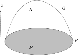
Figure 1: BCFT on $M$ and its dual $N$

Without loss of generality, we choose the following bulk action in this paper

$$I=\int_{N}d^{5}x\sqrt{|G|}\left(\hat{R}+12-\frac{1}{2}\left(\hat{\nabla}^{\mu}\hat{\phi}\hat{\nabla}_{\mu}\hat{\phi}+m^{2}\hat{\phi}^{2}\right)\right)+2\int_{Q}dx^{4}\sqrt{|\gamma|}\left(K-T+\frac{\xi}{2}\hat{\phi}\right),$$ (88)

where we have set $16\pi G_{N}=1$ and AdS radius $l=1$ for simplicity. Note that the Euclidean action is given by $I_{E}=-I$ with signature $(1,1,1,1)$. Here ($G_{\mu\nu}$, $\hat{R}$, $\hat{\nabla}_{\mu}$, $\hat{\phi}$) are the metric, scalar, covariant derivatives and Ricci scalar in the bulk $N$, ($\gamma_{ij},K$) are the induced metric and extrinsic curvature on the bulk boundary $Q$, $m$ is the mass of scalar field $\hat{\phi}$ and ($T,\xi$) are constant parameters of the theory. Note that $T$ can be regarded as holographic dual of the boundary entropy [25, 26, 27], while, as we will see later that, $\xi$ parameterizes the boundary condition of the scalar field. To have a well-defined action principle, one must impose suitable boundary conditions on $Q$. Following [25], we choose Neumann boundary conditions (NBC)

$$K_{ij}-(K-T+\frac{\xi}{2}\hat{\phi})\gamma_{ij}=0,$$ (89)

$$\hat{n}^{\mu}\hat{\nabla}_{\mu}\hat{\phi}-\xi=0,$$ (90)

where $\hat{n}^{\mu}$ is the outward-pointing normal vector on $Q$. Note that there are other choices of consistent boundary conditions [26, 27, 28], which we leave for future studies. From the action (88), we get equations of motion (EOM)

$$\hat{R}_{\mu\nu}-\frac{\hat{R}+12}{2}G_{\mu\nu}=\frac{1}{2}T_{\mu\nu},$$ (91)

$$(\hat{\nabla}^{\mu}\hat{\nabla}_{\mu}-m^{2})\hat{\phi}=0,$$ (92)

where $T_{\mu\nu}$ is the stress tensor of the scalar field

$$T_{\mu\nu}=\hat{\nabla}_{\mu}\hat{\phi}\hat{\nabla}_{\nu}\hat{\phi}-\frac{1}{2}G_{\mu\nu}\left(\hat{\nabla}^{\alpha}\hat{\phi}\hat{\nabla}_{\alpha}\hat{\phi}+m^{2}\hat{\phi}^{2}\right).$$ (93)

Near the AdS boundary, the scalar field behaves as

$$\hat{\phi}=z^{4-\Delta}\phi(x)++z^{\Delta}\phi_{(2\Delta-4)}(x),\quad z\to 0,$$ (94)

where $\phi$ is the boundary scalar discussed in section 2 and section 3, $\Delta=2+\sqrt{4+m^{2}}$ is the conformal dimension of the operator $O$ dual to $\hat{\phi}$. According to the dictionary of AdS/CFT [29, 30], we have

$$\langle O\rangle=\frac{1}{\sqrt{|g|}}\frac{\delta I}{\delta\phi}=(2\Delta-4)\phi_{(2\Delta-4)}+\cdots$$ (95)

where $\cdots$ denote finite and local functions of $(\phi,g_{ij},\psi_{(2\Delta-4)})$. Since we are interested in the ‘divergent terms’ (18) near the boundary, we can ignore these irrelevant $\cdots$ terms. For our purpose, we focus on the case $\Delta=3$, or equivalently,

$$m^{2}=-3,$$ (96)

which is above the Breitenlohner-Freedman stability bound $m^{2}>-4$ for asymptotic AdS₅.

Now the approach to derive the holographic one point function is straightforward. First we solve the coupled Einstein-scalar EOM (91) and (92) with the boundary conditions (89) and (90). Then we use the scalar solution to obtain the holographic one point function (95) from the asymptotic behaviour (94).

It is a non-trivial problem to find solutions which satisfy the EOM with the specified form of boundary conditions (BC). For examples, the usual AdS black holes are no longer solutions to AdS/BCFT generally, since they do not obey NBC (89). A systematic method based on derivative expansion was developed in [5, 31, 28]. Following [5, 31, 28], we take the following ansatz for the bulk metrics

$$ds^{2} = \frac{1}{z^{2}}\Big{[}dz^{2}+\left(1+\epsilon xX_{1}(\frac{z}{x})+\epsilon^{2}x^{2}X_{2}(\frac{z}{x})+\cdots\right)dx^{2}$$ (97)

$$+\left(\delta_{ab}-2\epsilon xK_{ab}(\frac{z}{x})+\epsilon^{2}x^{2}Q_{ab}(\frac{z}{x})+\cdots\right)dy^{a}dy^{b}\Big{]}$$

$$+O(\xi^{2})$$

and the bulk scalar field

$$\hat{\phi}=f_{0}(\frac{z}{x})+\epsilon\ xf_{1}(\frac{z}{x})+\epsilon^{2}x^{2}f_{2}(\frac{z}{x})+\epsilon^{3}x^{3}f_{3}(\frac{z}{x})+\cdots,$$ (98)

where $X_{n},K_{ab},Q_{ab},f_{n}$ are unknown functions to be determined and $\xi$ is the parameter for the scalar boundary condition (90). Note that we have introduced a parameter $\epsilon$ to label the order of derivative expansions with respect to $x$ or $z$. It should be set $\epsilon=1$ at the end of calculations. To get an asymptotic AdS background, we set the BC

$$X_{1}(0)=X_{2}(0)=0,\quad K_{ab}(0)=k_{ab},\quad Q_{ab}(0)=q_{ab},$$

$$\lim_{z\to 0}\frac{f_{0}(z)}{z}=0,\ \lim_{z\to 0}\frac{f_{1}(z)}{z}=\phi_{0},\quad\lim_{z\to 0}\frac{f_{2}(z)}{z}=\phi_{1},\quad\lim_{z\to 0}\frac{f_{3}(z)}{z}=\frac{1}{2}\phi_{2},\quad\mbox{etc.},$$ (99)

so that the metric and scalar on $M$ take expected forms in the Gauss normal coordinates

$$ds_{M}^{2}=dx^{2}+\left(\delta_{ab}-2\epsilon\ xk_{ab}+\epsilon^{2}x^{2}q_{ab}+\cdots\right)dy^{a}dy^{b},$$ (100)

$$\phi=\epsilon\phi_{0}+\epsilon^{2}x\phi_{1}+\epsilon^{3}\frac{x^{2}}{2}\phi_{2}+\cdots.$$ (101)

The powers of $\epsilon$ in (101) is understood from the fact that $\phi$, being the coefficient of $\hat{\phi}$ near $z=0$ as dedicated by (94), is already of order $\epsilon$. We also take the embedding function of bulk boundary $Q$ to be of the form

$$x=-\sinh\rho z+\epsilon\lambda_{1}z^{2}+\epsilon^{2}\lambda_{2}z^{3}+\cdots$$ (102)

where $\lambda_{n}$ are constants. Note that functions $X_{m},K_{ab},Q_{ab},f_{n},\lambda_{n}$ are functions of $\xi$.

5.1 Holographic Condensate

Let us first study the background solution with $\epsilon=0$. Substituting (98) into EOM (92,96) , we get

$$\left(s^{2}+1\right)s^{2}f_{0}^{\prime\prime}(s)+\left(2s^{2}-3\right)sf_{0}^{\prime}(s)+3f_{0}(s)=0,$$ (103)

which has the solution

$$f_{0}(s)=d_{1}\xi\frac{s^{3}}{\left(s^{2}+1\right)^{3/2}}+d_{2}\xi\frac{s\left(\sqrt{s^{2}+1}+s^{2}\tanh^{-1}(\sqrt{s^{2}+1})\right)}{\left(s^{2}+1\right)^{3/2}},$$ (104)

where $d_{1},d_{2}$ are integral constants and $s=\frac{z}{x}$. Imposing the NBC (90) on the bulk boundary $Q$ and DBC (5) on AdS boundary $M$, we fix the integral constants to be

$$d_{1}=-\frac{1}{3}\cosh^{3}\rho\,\coth\rho,\ \ \ d_{2}=0.$$ (105)

Thus, the scalar $f_{0}$ is of order $O(\xi)$. As a result, the scalar stress tensor (93) and thus the back reaction to the bulk geometry is of order $O(\xi^{2})$. This means that AdS metric is a solution to (91) only up to $O(\xi^{2})$. That is the reason why we add $O(\xi^{2})$ in the last line of bulk metric (97). For simplicity, we mainly focus on solutions up to $O(\xi)$ in this paper. We discuss briefly the effects of backreaction up to order $O(\xi^{2})$ to the metric and $O(\xi^{3})$ to the scalar field $\hat{\phi}$ in the appendix B.

Now we are ready to derive the leading term of one point function. From (95), (98) and (104), we obtain

$$\langle O\rangle=\frac{2d_{1}\xi}{x^{3}}+O(1/x^{2},\xi^{2}).$$ (106)

Comparing with (26), we read off the central charge

$$b_{3}=\frac{d_{1}\xi}{6}=-\frac{\xi}{18}\cosh^{3}\rho\,\coth\rho+O(\xi^{2})$$ (107)

Following the same procedure, we can solve for the bulk solutions to (97) and (98) order in order in $\epsilon$ and derive the sub-leading terms of the one point function. Since the calculations are quite complicated, we will first study below some special cases and then list the general results. In following subsections, we will determine the bulk solution up to order $\epsilon^{2}$ and linear order in $\xi$.

5.1.1 Free-Field Limit

To warm up, let us first study so-called Free-Field Limit. It is noticed that, when the brane tension vanishes $T=0$, holographic Weyl anomaly [32], norm of displacement operator [28, 33] and their two point functions [33, 34] all exactly match those of free theories. So we call $T=0$ the free-field limit. When there are scalars, a natural choice of the free-field limit would be to take $\xi=0$ in addition to $T=0$. Equivalently, the boundary conditions become

$$K_{ij}-K\gamma_{ij}=0,$$ (108)

$$\hat{n}^{\mu}\hat{\nabla}_{\mu}\hat{\phi}=0.$$ (109)

Below we will show that the above boundary conditions can indeed produce the form of one point function for free BCFT.

First from (98,104,105), we notice that $\hat{\phi}\sim O(\epsilon)$ when $\xi=0$. As a result, the back reaction due to scalars to the bulk metric is of order $O(\epsilon^{2})$. Fortunately, to derive one point function up to $O(\epsilon^{2})$ ($O(1/x)$), we do not need the bulk metric of order $O(\epsilon^{2})$. That is because, from EOM (92) and $\hat{\phi}\sim O(\epsilon)$, the order $O(\epsilon^{2})$ terms of the bulk metric affect only the order $O(\epsilon^{3})$ terms of the bulk scalar and thus are irrelevant for the one point function up to order $O(\epsilon^{2})$. This means we can ignore the back reaction of scalars on the metric in the free-field limit $\xi=0$.

On this, we recall the metric without scalars were obtained in [5], where the bulk metric is given by

$$ds^{2}=\frac{1}{z^{2}}\Big{[}dz^{2}+\big{(}1+x^{2}\epsilon^{2}X(\frac{z}{x})\big{)}dx^{2}$$

$$+\big{(}\delta_{ab}-2x\epsilon\bar{k}_{ab}f(\frac{z}{x})-2x\epsilon\frac{k}{3}\delta_{ab}+x^{2}\epsilon^{2}Q_{ab}(\frac{z}{x})\big{)}dy^{a}dy^{b}\Big{]}$$

$$+O(\epsilon^{3}),$$ (110)

and the embedding function of $Q$ is given by

$$x=-\sinh(\rho)z+\epsilon\frac{k\cosh^{2}\rho}{6}z^{2}+\epsilon^{2}\lambda_{2}z^{3}+O(\epsilon^{3})$$ (111)

Here $k_{ab}=\text{diag}(k_{1},k_{2},k_{3})$, $T=3\tanh\rho$, $f(s)$ is given by

$$f(s)=1+2\alpha_{1}-\frac{\alpha_{1}\left(s^{2}+2\right)}{\sqrt{s^{2}+1}},$$ (112)

$$\alpha_{1}=\frac{-1}{2(1+\tanh\rho)},$$

and $X,Q_{ab},\lambda_{2}$ are complicated functions, which can be found in the appendix of [5] . As mentioned above, in the free-field limit, we do not need either $X,Q_{ab},\lambda_{2}$ which are of order $O(\epsilon^{2})$ or a non-vanishing tension $T=3\tanh\rho$. However, for the convenience of following sections, we will give the general results below by first studying the general case with $T=3\tanh\rho$ and then we will take the free-field limit $T\to 0$ at the end of calculations.

Substituting bulk metric (5.1.1) and scalar (98) with $f_{0}=0$ into EOM (92), we obtain

$$f_{1}(s)=s\left(\frac{d_{3}}{\sqrt{s^{2}+1}}+d_{4}\right),$$ (113)

$$f_{2}(s)=\frac{s\left(d_{3}k+2d_{6}(s^{2}+1)\right)}{2\sqrt{s^{2}+1}}+d_{5}s.$$ (114)

Imposing DBC (5) on AdS boundary $z=0$, we get

$$d_{4}=\phi_{0}-d_{3},\ \ d_{6}=-\frac{1}{2}d_{3}k-d_{5}+\phi_{1}.$$ (115)

Imposing NBC (109) on bulk boundary $Q$, we obtain

$$d_{3}=\frac{\phi_{0}\coth\rho}{\coth\rho-\text{csch}^{2}\rho+1},\quad d_{5}=\frac{k\phi_{0}(-\sinh(2\rho)+\cosh(2\rho)-3)+3\phi_{1}\sinh(2\rho)}{3(\sinh(2\rho)+\cosh(2\rho)-3)}.$$ (116)

Substituting bulk scalar solution (113) and (114) into (95) and (98), we obtain the one point function

$$\langle O\rangle=-\frac{d_{3}}{x^{2}}\epsilon-\frac{d_{3}k+d_{5}-\phi_{1}}{x}\epsilon^{2}+O\left(\epsilon^{3},\xi\right).$$ (117)

In the free-field limit $T=\rho=0$, it becomes

$$\langle O\rangle=-\frac{\left(\frac{k}{3}\phi_{0}-\phi_{1}\right)}{x}\epsilon^{2}+O\left(\epsilon^{3},\xi\right),$$ (118)

which takes the same form (27) as that of the free theories [2] with all the boundary charges vanish: $b_{i}=0$. Comparing with (27) and using $n^{i}\nabla_{i}\phi=-\phi_{1}+O(x)$, we get the bulk central charge

$$a_{1}=\frac{1}{2}.$$ (119)

Note that the bulk central charge is independent of boundary conditions, so (119) is exact and gets no corrections from $\epsilon$ and $\xi$.

5.1.2 No-Scalar Limit

Let us go on to investigate the no-scalar limit. By ‘no scalar’ we mean there is no boundary scalar, i.e., $\phi=0$, but the bulk scalar $\hat{\phi}$ can be non-zero. Now we have $\hat{\phi}\sim O(\xi)$, which back react the bulk metric at order $O(\xi^{2})$. Since we mainly focus on solutions linear in $\xi$, we can ignore the back reaction due to scalars to the bulk metrics. Note that we have $\hat{\phi}\sim O(\xi)$ in no-scalar limit, while $\hat{\phi}\sim O(\epsilon)$ in free-field limit. As a result, unlike the case of free-field limit, in no-scalar limit we need bulk metrics (5.1.1) of order $O(\epsilon^{2})$ in order to get the one point function of order $O(\epsilon^{2})$.

Solving EOM (92) with bulk metric (5.1.1) and impose the DBC (5) with $\phi_{0}=\phi_{1}=0$, we obtain $f_{0}$ (104) with $d_{2}=0$ and

$$f_{1}(s)=\frac{1}{2}d_{1}ks\left(1-\frac{1}{\left(s^{2}+1\right)^{3/2}}\right)+e_{1}s\left(\frac{1}{\sqrt{s^{2}+1}}-1\right)$$ (120)

and

$$f_{2}(s) = \frac{q\left(-\left(d_{1}s^{3}\left(3s^{2}+2\right)\right)\right)}{6\left(s^{2}+1\right)^{5/2}}-\frac{k\left(e_{1}s^{3}\right)}{2\sqrt{s^{2}+1}}-\frac{e_{2}\left(s^{3}-\sqrt{s^{2}+1}s+s\right)}{\sqrt{s^{2}+1}}$$ (121)

$$+\text{Tr}k^{2}\left(\frac{d_{1}s^{3}\left(5s^{4}+21s^{2}+14\right)}{8\left(s^{2}+1\right)^{5/2}}-3h_{1}(s)\right)+k^{2}h_{1}(s)$$

with

$$h_{1}(s) = \frac{d_{1}s}{360\left(s^{2}+1\right)^{5/2}}\left[15s^{2}(3s^{4}+12s^{2}+8)-30\alpha_{1}^{2}s^{2}(3s^{2}+2)\log\left(s^{2}+1\right)\right.$$ (122)

$$-12\alpha_{1}\left(2s^{6}-9s^{4}+4(5\sqrt{s^{2}+1}-6)s^{2}+8(\sqrt{s^{2}+1}-1)\right)$$

$$\left.+4\alpha_{1}^{2}\left(14s^{6}+87s^{4}-8(15\sqrt{s^{2}+1}-19)s^{2}-48(\sqrt{s^{2}+1}-1)\right)\right],$$

where $d_{1}$ is (105), $\alpha_{1}$ is given by (112) and $e_{1},e_{2}$ are integral constants. Imposing the NBC (90), we fix the integral constants

$$e_{1}=-\xi\frac{k}{6}\cosh^{3}\rho\,\coth\rho$$ (123)

and

$$e_{2} = \xi\frac{\left(3\text{Tr}k^{2}-k^{2}\right)\coth\rho\,{\rm csch}^{2}\rho}{1080(\coth\rho-2)(\coth\rho+1)^{2}}$$ (124)

$$\left(20\sinh\rho+13\sinh(3\rho)+3\sinh(5\rho)-22\cosh\rho-4\cosh(3\rho)\right)$$

Substituting the above scalar solution into (95), we obtain the one point function for $\phi=0$ (28) with the central charges $b_{3}$ given by (107) and

$$b_{4}=-\xi\frac{-11\sinh(2\rho)-8\sinh(4\rho)+8\cosh(2\rho)+7\cosh(4\rho)+1}{90(-5\sinh\rho+3\sinh(3\rho)+3\cosh\rho-3\cosh(3\rho))}+O(\xi^{2}).$$ (125)

Note that there are four independent terms but only two parameters in (28). It is non-trivial to have consistent solutions (107) and (125). This is a strong support of our results.

5.1.3 Flat Limit

In this subsection, we consider the back reaction of scalars. For simplicity, we focus on the flat space with flat boundary, i.e., $k_{ab}=q_{ab}=0$. We denote this case as the ‘flat limit’. Since the calculations are quite similar to those of above subsections, below we only show the key steps.

In the flat limit, the ansatz for bulk metrics and bulk scalar can be simplified as

$$ds^{2} = \frac{1}{z^{2}}\Big{[}dz^{2}+\left(1+\epsilon\xi xX_{1e}(\frac{z}{x})+\epsilon^{2}x^{2}\left(X_{2}(\frac{z}{x})+\xi X_{2e}(\frac{z}{x})\right)\right)dx^{2}$$ (126)

$$+\delta_{ab}\left(1+\epsilon\xi xg_{1e}(\frac{z}{x})+\epsilon^{2}x^{2}\left(g_{2}(\frac{z}{x})+\xi g_{2e}(\frac{z}{x})\right)\right)dy^{a}dy^{b}\Big{]}$$

$$+O(\xi^{2},\epsilon^{3})$$

and

$$\hat{\phi}=f_{0}(\frac{z}{x})+\epsilon\ xf_{1}(\frac{z}{x})+\epsilon^{2}x^{2}\left(f_{2}(\frac{z}{x})+\xi f_{2e}(\frac{z}{x})\right)+O(\xi^{2},\epsilon^{3}),$$ (127)

where $f_{0}$ is given by (104,105) up to order $O(\xi)$. Solving the coupled Einstein-scalar EOM (91), (92) and the DBC (5) with $k_{ab}=q_{ab}=0$, we obtain for the bulk scalar

$$f_{1}(s)=s\left(d_{3}(\frac{1}{\sqrt{s^{2}+1}}-1)+\phi_{0}\right),$$ (128)

$$f_{2}(s)=s\left(\sqrt{s^{2}+1}\left(\phi_{1}-d_{5}\right)+d_{5}\right)$$ (129)

and

$$f_{2e}(s)=\frac{s\left(-s^{2}+\sqrt{s^{2}+1}-1\right)}{\sqrt{s^{2}+1}}d_{7}$$

$$+\frac{d_{1}s}{48\left(s^{2}+1\right)^{5/2}}\Big{[}-2s^{2}\left(15(s^{2}+2)s^{2}+16\right)\phi_{0}^{2}$$

$$+2d_{3}\left(25s^{6}+33s^{4}+(26\sqrt{s^{2}+1}-15)s^{2}+17(\sqrt{s^{2}+1}-1)\right)\phi_{0}$$

$$+d_{3}^{2}\left(-19s^{6}-52\sqrt{s^{2}+1}s^{2}+54s^{2}-34\sqrt{s^{2}+1}-6s^{4}\left(\log(s^{2}+1)+2\right)+34\right)\Big{]}.$$ (130)

Imposing the NBC (89), (90), we obtain the integral constants $d_{1}$ (105) and

$$d_{3}=\frac{-\phi_{0}\sinh\rho\cosh\rho}{(\cosh\rho-2\sinh\rho)(\sinh\rho+\cosh\rho)},$$ (131)

$$d_{5}=\frac{\phi_{1}\sinh(2\rho)}{\sinh(2\rho)+\cosh(2\rho)-3},$$

$$d_{7}=\frac{\phi_{0}^{2}\text{csch}^{5}\rho}{9216(\coth\rho-2)^{2}(\coth\rho+1)^{2}}\Big{[}688-1106\sinh(2\rho)-258\sinh(4\rho)+70\sinh(6\rho)$$

$$\ \ \ \ +\sinh(8\rho)+616\cosh(2\rho)-192\cosh(4\rho)-104\cosh(6\rho)+16\cosh(8\rho)\Big{]}.$$ (132)

Please see appendix B for the solutions to the bulk metric (126) and the embedding function of $Q$ (102) . Substituting the above scalar solutions into (95), we obtain the one point function in flat limit

$$\langle O\rangle=\frac{12b_{3}}{x^{3}}+\frac{3b_{2}\phi}{x^{2}}\epsilon-\frac{2a_{1}\nabla_{n}\phi+3b_{1}\phi^{2}}{x}\epsilon^{2}+O(x^{0},\ln x),$$ (133)

where $b_{3}$ is given by (107), $a_{1}$ is given by (119) and

$$b_{1}=-\xi\frac{\text{csch}^{3}\rho}{1152(\coth\rho-2)^{2}}\Big{(}44+57\cosh(2\rho)+20\cosh(4\rho)$$

$$\ \ \ \ \ \ \ \ -61\sinh(2\rho)-30\sinh(4\rho)-5\sinh(6\rho)+7\cosh(6\rho)\Big{)}+O(\xi^{2}),$$ (134)

$$b_{2}=\frac{\sinh\rho\cosh\rho}{3(\cosh\rho-2\sinh\rho)(\sinh\rho+\cosh\rho)}+O(\xi^{2}).$$ (135)

Note that $a_{1}$ and $b_{3}$ derived in the flat limit (133) agree with those obtained in free-field limit and no-scalar limit. This can be regarded as a double check of our results. Now we have got all of the boundary central charges $b_{1}$ (5.1.3), $b_{2}$ (135), $b_{3}$ (107) and $b_{4}$ (125) in holographic BCFT (88).

So far, we have verified the one point function (26) in three special cases. The generalization to general case is straightforward. However, the general solutions to the bulk metric (97) and bulk scalar (98) are quite complicated, we do not list them in this paper. The interested reader can obtain them straightforwardly with the help of Mathematica. Besides, we focus on solutions in the linear order of $\xi$ in this section. Please refer to appendix B for solutions in higher orders of $\xi$.

5.2 Holographic Weyl Anomaly

In this subsection, we investigate the holographic Weyl Anomaly due to the scalar background. In particular, we reproduce the four boundary central charges $b_{1},b_{2},b_{3},b_{4}$ obtained in section 4.1 and verify the universal relations between one point function (26) and Weyl anomaly (9).

5.2.1 Bulk Weyl Anomaly

Let us first consider the bulk contributions to Weyl anomaly, where we can ignore the boundaries. For this case we can apply the standard method [35] to derive the holographic Weyl Anomaly. Due to the non-trivial back reactions, the case with boundaries is more subtle, and we leave a careful study of it in next subsection.

Following [35], we take the Fefferman-Graham gauge for the asymptotically $AdS_{5}$ metric

$$ds^{2}=\frac{d\rho^{2}}{4\rho^{2}}+\frac{\hat{g}_{ij}(x,\rho)dx^{i}dx^{j}}{\rho},$$ (136)

where $\hat{g}_{ij}=g_{ij}+\rho g_{(1)ij}+\cdots$ and $\rho=z^{2}$. Using the EOM (91) together with (94) with $\Delta=3$ and (136), we obtain

$$g^{(1)}_{ij}=-\frac{1}{2}R_{ij}+\frac{1}{12}(R-\phi^{2})g_{ij}.$$ (137)

Substituting the bulk metric (136,137) and bulk scalar (94) with $\Delta=3$ into action (88), selecting UV logarithmic divergent terms, we obtain the bulk contributions to holographic Weyl anomaly

$$\mathcal{\hat{A}}_{\text{bulk}}=(I)_{\log\frac{1}{\epsilon}}=\frac{-1}{2}\int_{M}\sqrt{g}[(\nabla\phi)^{2}+\frac{1}{6}R\phi^{2}+\frac{1}{6}\phi^{4}]$$ (138)

in signature $(1,1,1,1)$ or $(-1,1,1,1)$. In signature $(1,-1,-1,-1)$, the definition of Weyl anomaly $\mathcal{A}=\langle T^{i}_{\ i}\rangle$ change sign. That is because $T^{i}_{\ i}$ differs by a minus sign in different signature. Please see appendix A for more clarifications. Transform into signature $(1,-1,-1,-1)$, the bulk Weyl anomaly becomes

$$\mathcal{A}_{\text{bulk}}=(I)_{\log\epsilon}=\frac{1}{2}\int_{M}\sqrt{g}[-(\nabla\phi)^{2}+\frac{1}{6}R\phi^{2}+\frac{1}{6}\phi^{4}],$$ (139)

from which one can read off the bulk central charges

$$a_{1}=\frac{1}{2},\quad a_{2}=\frac{1}{12}$$ (140)

which agree with (119). To avoid confusion, by central charges we always refer to those coefficients appearing in the Weyl anomaly (9) in signature $(1,-1,-1,-1)$.

5.2.2 Boundary Weyl Anomaly

Let us turn to discuss the boundary contributions to holographic Weyl anomaly. To derive boundary Weyl anomaly of $O(\epsilon^{3})$, one can work out bulk solutions (97,98) of order $O(\epsilon^{3})$ and then select the UV logarithmic divergent terms in the action. However, the $O(\epsilon^{3})$ solutions are quite complicated. Instead, we use a simpler method developed by [36], which needs only bulk solutions of order $O(\epsilon^{2})$.

Consider the variation of the gravitational action (88), we have

$$\delta I=\int_{N}\text{EOM}+\int_{Q}\sqrt{\gamma}\left[\left((K-T+\frac{\xi}{2}\hat{\phi})\gamma^{ij}-K^{ij}\right)\delta\gamma_{ij}+(\xi-\hat{n}^{\mu}\hat{\nabla}_{\mu}\hat{\phi})\delta\hat{\phi}\right]$$

$$\ \ \ \ \ +\int_{M}\sqrt{g}\left(\frac{1}{2}T^{ij}_{\text{non-ren}}\delta g_{ij}+O_{\text{non-ren}}\delta\phi\right),$$ (141)

where the first line of (5.2.2) vanishes due to EOM and NBC (89,90), $T^{ij}_{\text{non-ren}}$ and $O_{\text{non-ren}}$ are non-renormalized stress tensor and one point function of scalar, respectively. To get renormalized stress tensor and scalar operator, we can subtract a reference one without boundaries. For the reference action without bulk boundary $Q$, we have

$$\delta I_{0}=\int_{M}\sqrt{g}\left(\frac{1}{2}T^{ij}_{0}\delta g_{ij}+O_{0}\delta\phi\right),$$ (142)

where the integration is over the same region $M$ as in (5.2.2). Consider the difference of (5.2.2) and (142), we get

$$\delta(I-I_{0})=\int_{M}\sqrt{g}\left(\frac{1}{2}T^{ij}_{\text{holo}}\delta g_{ij}+O_{\text{holo}}\delta\phi\right),$$ (143)

where $T^{ij}_{\text{holo}}:=T^{ij}_{\text{non-ren}}-T^{ij}_{0}$ is the renormalized holographic stress tensor and similarly for $O_{\text{holo}}$. Select the UV logarithmic divergent term of above equation and notice that $I$ and $I_{0}$ have the same bulk Weyl anomaly, we obtain

$$\delta\mathcal{A}|_{\partial M}=\delta(I-I_{0})_{\log\epsilon}=\int_{M}\sqrt{g}\left(\frac{1}{2}T^{ij}_{\text{holo}}\delta g_{ij}+O_{\text{holo}}\delta\phi\right)\Big{|}_{\log\epsilon},$$ (144)

which is just the holographic derivation of (20). The key point here is that the left hand of (144) is a total variation. As a result, the boundary Weyl anomaly can be obtained by integrating $\delta g_{ij}$ and $\delta\phi$. Since we are interested in the scalar contributions to Weyl anomaly, we can turn off the variation of metric. By integrating (144), we can obtain Weyl anomaly up to some irrelevant bulk terms such as $\mathcal{A}_{2}$ (11). Here by ‘irrelevant terms’, we mean ‘integration constant’ terms which do not contribute to $\delta\mathcal{A}|_{\partial M}$. (144) shows that it is sufficient to derive $\delta\mathcal{A}|_{\partial M}$ of $O(\epsilon^{3})$ from $O_{\text{holo}}$ of $O(\epsilon^{2})$, due to the fact that $\phi$ is of $O(\epsilon)$.

Recall that, in section 4.1, we have obtained the holographic scalar operator $O_{\text{holo}}$ as (26) with boundary central charges given by (107, 125, 5.1.3, 135). Substituting $O_{\text{holo}}$ into (144) and integrating $\delta\phi$, we get the holographic boundary Weyl anomaly as (9) with boundary central charges given by (107, 125, 5.1.3, 135). This is just a turn-around of the logic of section 3.1. Thus there is no need to repeat the calculations here. Note that, from (144) one cannot derive all of the bulk Weyl anomaly.

6 Holographic Story II: CFT without Boundary

In this section, we give a holographic derivation of the anomalous transformation rule (33) for the scalar operator $O$ under Weyl transformation.

According to [37] , the Weyl transformations $g^{\prime}_{ij}=e^{-2\sigma}g_{ij}$ can be realized by suitable bulk diffeomorphisms. Inspired by [37], we take the ansatz [38]

$$\rho=\rho^{\prime}e^{2\sigma(x^{\prime})}\left(1+\sum_{n=1}^{\infty}\rho^{\prime n}b_{(n)}(x^{\prime})\right)$$ (145)

$$x^{i}=x^{\prime i}+\sum_{n=1}^{\infty}\rho^{\prime n}a^{i}_{(n)}(x^{\prime})$$ (146)

which is non-perturbative in the conformal factor. We require that the above diffeomorphisms leave the form of bulk metric (136) invariant, i.e.,

$$G^{\prime}_{\rho\rho}=\frac{\partial X^{\mu}}{\partial\rho^{\prime}}\frac{\partial X^{\nu}}{\partial\rho^{\prime}}G_{\mu\nu}=\frac{1}{4\rho^{\prime 2}},$$ (147)

$$G^{\prime}_{\rho i}=\frac{\partial X^{\mu}}{\partial\rho^{\prime}}\frac{\partial X^{\nu}}{\partial x^{\prime i}}G_{\mu\nu}=0.$$ (148)

Substituting (145,146) into (148), we obtain [37, 38]

$$a_{(1)}^{i}=-\frac{1}{2}g^{\prime ij}\partial_{j}\sigma,$$ (149)

$$b_{(1)}=-\frac{1}{2}g^{\prime ij}\partial_{i}\sigma\partial_{j}\sigma,$$ (150)

where $g^{\prime}{}^{ij}=e^{2\sigma}g^{ij}$ is non-perturbative in the scale factor.

Now we are ready to derive the transformation law of scalar operator $O$ under Weyl transformation. Under the diffeomorphisms (145,146), the bulk scalar (94) becomes

$$\hat{\phi^{\prime}}(\rho^{\prime},x^{\prime})=\hat{\phi}(\rho,x)=\rho^{\frac{1}{2}}\phi(x)+\rho^{\frac{3}{2}}[\phi_{(2)}(x)+\psi_{(2)}(x)\ln\rho]+O(\rho^{\frac{3}{2}})$$

$$= \rho^{\prime\frac{1}{2}}e^{\sigma}(1+\frac{1}{2}\rho^{\prime}b_{(1)})\left(\phi(x^{\prime})+\rho^{\prime}a_{(1)}^{i}\partial_{i}\phi(x^{\prime})\right)$$

$$+\rho^{\prime\frac{3}{2}}e^{3\sigma}(1+\frac{3}{2}\rho^{\prime}b_{(1)})\Big{(}\phi_{(2)}(x^{\prime})+\psi_{(2)}(x^{\prime})\ln\rho^{\prime}+2\sigma\psi_{(2)}(x^{\prime})\Big{)}+O(\rho^{\prime\frac{3}{2}})$$

$$= \rho^{\prime\frac{1}{2}}[e^{\sigma}\phi(x^{\prime})]+O(\rho^{\prime\frac{3}{2}})$$

$$+\rho^{\prime\frac{3}{2}}\left[e^{\sigma}\left(a_{(1)}^{i}\partial_{i}\phi(x^{\prime})+\frac{1}{2}b_{(1)}\phi(x^{\prime})\right)+e^{3\sigma}\Big{(}\phi_{(2)}(x^{\prime})+2\sigma\psi_{(2)}(x^{\prime})+\psi_{(2)}(x^{\prime})\ln\rho^{\prime}\Big{)}\right].$$

From the above equation and (94) , we can read off the transformation rules

$$\phi^{\prime}=e^{\sigma}\phi,$$ (153)

$$\psi^{\prime}_{(2)}=e^{3\sigma}\psi_{(2)},$$

$$\phi^{\prime}_{(2)}=e^{3\sigma}\phi_{(2)}+e^{\sigma}\left(a_{(1)}^{i}\partial_{i}\phi(x^{\prime})+\frac{1}{2}b_{(1)}\phi(x^{\prime})\right)+e^{3\sigma}\Big{(}2\sigma\psi_{(2)}(x^{\prime})\Big{)}$$ (154)

According to the standard approach, $\psi_{(2)}$ can be obtained from either EOM (92) or the variation of holographic Weyl anomaly (139). Applying both methods, we get

$$\psi_{(2)}=-\frac{1}{4}\nabla^{2}\phi+\frac{1}{24}R\phi+\frac{1}{12}\phi^{3},$$ (155)

$$\psi^{\prime}_{(2)}=-\frac{1}{4}\nabla^{\prime 2}\phi^{\prime}+\frac{1}{24}R^{\prime}\phi^{\prime}+\frac{1}{12}\phi^{\prime 3}.$$ (156)

One can check that (155) and (156) obey the transformation rule (153), which is a test of our results. Substituting (149,150,156) into (154) and noting that $\langle O\rangle=2\phi_{(2)}$, we finally obtain the Weyl transformation rule

$$\langle O\rangle=e^{-3\sigma}\langle O\rangle^{\prime}+\nabla(\sigma\nabla\phi)-\frac{1}{6}\phi R\sigma+\frac{1}{2}\phi(\nabla\sigma)^{2}-\frac{1}{3}\phi^{3}\sigma,$$ (157)

in signature $(-1,1,1,1)$ or $(1,1,1,1)$. Transforms into signature $(1,-1,-1,-1)$, $\nabla(\sigma\nabla\phi),(\nabla\sigma)^{2}$ change sign and (157) agrees with the field-theoretical result (33) with central charges (140).

7 Conclusions and Discussions

In this paper, we have investigated anomalous Fermi condensation (one point function of scalar operator) due to Weyl anomaly. We obtain general form of Weyl anomaly due to a background scalar for 4d BCFTs, which consequently leads to two kinds of anomalous Fermi condensation. The first kind occurs near a boundary, while the second kind appears in conformally flat spacetime without boundaries. It is interesting that the first kind of Fermi condensation could be non-zero in flat spacetime and even if there is no background scalar. While the second kind of Fermi condensation only appears in a curved spacetime with non-zero background scalar. We verify our results with free BCFT and holographic BCFT. In particular, we consider carefully the back reaction to the AdS geometry due to the scalar field and reproduce precisely the shape and curvature dependence of the field theoretic Fermi condensate from the holographic one point function.

For simplicity, we focus on CFT/BCFTs in four dimensions in this paper. It is interesting to generalize our works to general dimensions. Besides, it is also interesting to study Fermi condensation for general QFT. For QFT, more possible terms are allowed in Weyl anomaly, which would correct the results of anomalous Fermi condensation. We hope to address these problems in future.

Appendix A Weyl Anomaly in Different Signatures

In this appendix, we clarify that Weyl anomaly $<T^{i}_{\ i}>$ differs by a minus sign in different signature. First, let us stress that the action is independent of the choice of signature. In signature $(-1,1,1,1)$, the stress tensor is defined by [4]

$$\delta I=\frac{1}{2}\int_{M}\sqrt{|g|}\hat{T}^{ij}\delta\hat{g}_{ij},$$ (158)

while in signature $(1,-1,-1,-1)$ the stress tensor is defined by [3]

$$\delta I=-\frac{1}{2}\int_{M}\sqrt{|\hat{g}|}T^{ij}\delta g_{ij},$$ (159)

where $\hat{g}_{ij}=-g_{ij}$. From (158) and (159), we notice that $T^{ij}=\hat{T}^{ij}$ and hence the Weyl anomaly in different signature differs by a minus sign

$$\langle T^{ij}\rangle g_{ij}=-\langle\hat{T}^{ij}\rangle\hat{g}_{ij}.$$ (160)

The Euclidean theory is related to the theory with signature $(-1,1,1,1)$ by a Wick rotation, therefore the Weyl anomaly in Euclidean theory is also different by a minus sign from the Weyl anomaly in the signature $(1,-1,-1,-1)$.

For the convenience of readers, let us list some important formulas in both signature. The action of Dirac field takes the form

$$I=\int_{M}\sqrt{|g|}\left(\bar{\psi}i\gamma^{i}\nabla_{i}\psi+\phi\bar{\psi}\psi\right),$$ (161)

where $\bar{\psi}=\psi^{+}\gamma^{0}$, $(\gamma^{0})^{+}=\gamma^{0}$, $(\gamma^{a})^{+}=-\gamma^{a}$ and the gamma matrix obeys

$$\{\gamma^{i},\gamma^{j}\}=2\eta\ g^{ij}.$$ (162)

Here $\eta=-1$ for signature $(-1,1,1,1)$ [4] and $\eta=1$ for signature $(1,-1,-1,-1)$ [3]. The key relation (20) becomes

$$\eta(\delta_{\phi}\mathcal{A})_{\partial M}=\left(\int_{M}\sqrt{|g|}\langle\bar{\psi}\psi\rangle\delta\phi\right)_{\log\epsilon}.$$ (163)

To summarize, the action, the stress tension $T_{ij}$, the gamma matrices $\gamma^{i}$ and the Fermi condensation $\langle\bar{\psi}\psi\rangle$ are the same, while the metric $g_{ij}$ and the Weyl anomaly $\langle T^{i}_{\ i}\rangle$ differ by a minus sign in different signatures. Note that we take signature $(1,-1,-1,-1)$ from section 1 to section 4, while signature $(-1,1,1,1)$ or $(1,1,1,1)$ in section 5 and section 6 in this paper. To avoid confusion, we denote Weyl anomaly in signature $(1,-1,-1,-1)$ by $\mathcal{A}$ and Weyl anomaly in signature $(-1,1,1,1)$ by $\mathcal{\hat{A}}$ in the main text of this paper.

Appendix B Solutions in the Flat Limit

In the flat limit, the bulk metric is given by (126) with

$$X_{1e}(s)=d_{1}\left(\sqrt{s^{2}+1}\left(d_{3}-\phi_{0}\right)+\frac{d_{3}-\phi_{0}}{\sqrt{s^{2}+1}}-\frac{d_{3}}{2\left(s^{2}+1\right)}-\frac{1}{2}d_{3}\log\left(s^{2}+1\right)-\frac{3d_{3}}{2}+2\phi_{0}\right),$$ (164)

$$X_{2}(s)=-\frac{d_{3}}{2}\left(-s^{2}+2\sqrt{s^{2}+1}-2\right)\phi_{0}+d_{3}^{2}\left(-\frac{s^{2}}{4}+\sqrt{s^{2}+1}-\frac{1}{4}\log\left(s^{2}+1\right)-1\right)-\frac{1}{12}s^{2}\phi_{0}^{2},\;\;\;\;$$ (165)

$$X_{2e}(s)=\frac{d_{1}}{2}\left[d_{5}\Big{(}\frac{4\left(s^{2}+2\right)(\sqrt{s^{2}+1}-1)}{\sqrt{s^{2}+1}}-\left(s^{2}+4\right)\log\left(s^{2}+1\right)\Big{)}+\phi_{1}\left(\left(s^{2}+4\right)\log\left(s^{2}+1\right)-4s^{2}\right)\right],\;\;\;\;$$ (166)

$$g_{1e}(s)=\frac{d_{1}\left(4\left(s^{2}+1\right)^{3/2}\left(d_{3}-\phi_{0}\right)+4\left(s^{2}+1\right)^{5/2}\left(d_{3}-\phi_{0}\right)+2d_{3}\left(s^{2}+1\right)-d_{3}\right)}{12\left(s^{2}+1\right)^{2}}+d_{1}\left(\frac{2\phi_{0}}{3}-\frac{3d_{3}}{4}\right),\;\;\;\;$$ (167)

$$g_{2}(s)=\frac{1}{24}\Big{(}-4d_{3}(-s^{2}+2\sqrt{s^{2}+1}-2)\phi_{0}+\frac{d_{3}^{2}\left(-3s^{4}+4(2\sqrt{s^{2}+1}-3)s^{2}+8(\sqrt{s^{2}+1}-1)\right)}{s^{2}+1}-2s^{2}\phi_{0}^{2}\Big{)},\;\;$$ (168)

$$g_{2e}(s)=\frac{d_{1}\Big{(}d_{5}-\phi_{1}\left(s^{2}\left(s^{2}+2\right)-2\left(s^{2}+1\right)\log\left(s^{2}+1\right)\right)\Big{)}}{4\left(s^{2}+1\right)}.$$ (169)

The embedding function of $Q$ takes the form (102)

$$x=-\sinh\rho z+\epsilon\xi\lambda_{1e}z^{2}+\epsilon^{2}(\lambda_{2}+\xi\lambda_{2e})z^{3}+\cdots$$ (170)

with

$$\lambda_{1e} = \frac{\phi_{0}\cosh^{3}\rho}{288(7\sinh\rho-\sinh(3\rho)+\cosh\rho-\cosh(3\rho))}\Big{[}16\cosh\rho-96\cosh(3\rho)+16\cosh(5\rho)$$ (171)

$$+\sinh\rho(-92+6\log(\coth^{2}\rho))+\sinh(3\rho)(-84+3\log(\coth^{2}\rho))$$

$$+\sinh(5\rho)(16-3\log(\coth^{2}\rho))\Big{]},$$

$$\lambda_{2} = \frac{\phi_{0}^{2}\sinh\rho}{2304(\cosh\rho-2\sinh\rho)^{2}(\sinh\rho+\cosh\rho)^{2}}\Big{[}12+28\sinh(2\rho)+112\sinh(4\rho)-20\sinh(6\rho)$$ (172)

$$+\cosh(2\rho)\left(4-3\log(\coth^{2}\rho)\right)+\cosh(4\rho)\left(100-6\log(\coth^{2}\rho)\right)$$

$$-\cosh(6\rho)(20-3\log(\coth^{2}\rho))+6\log\left(\coth^{2}\rho\right)\Big{]},\;\;$$

$$\lambda_{2e} = \frac{\phi_{1}\cosh^{4}(\rho)}{72(\sinh(2\rho)+\cosh(2\rho)-3)}\Big{[}48-8\sinh(2\rho)+4\sinh(4\rho)+3\log(\coth^{2}\rho)$$ (173)

$$-2\cosh(2\rho)\left(9\log(\coth^{2}\rho)+10\right)+\cosh(4\rho)\left(3\log(\coth^{2}\rho)+4\right)\Big{]}.$$

Appendix C Back Reaction due to Scalar BC

In the main text of the paper, we focus on solutions in the linear order of $\xi$, where $\xi$ labels the NBC (90) of the scalar field. In this appendix, we discuss solutions in higher orders of $\xi$ briefly. For simplicity, we focus on both the flat limit with $k_{ab}=q_{ab}=0$ and the no-scalar limit $\phi=0$. Then the ansatz for bulk metric, bulk scalar and embedding function of $Q$ become

$$ds^{2}=\frac{1}{z^{2}}\Big{[}dz^{2}+\left(1+\xi^{2}X_{e}(\frac{z}{x})\right)dx^{2}+\delta_{ab}\left(1+\xi^{2}\ g_{e}(\frac{z}{x})\right)dy^{a}dy^{b}\Big{]}+O(\xi^{3},\epsilon)$$ (174)

$$\hat{\phi}=f_{0}(\frac{z}{x})+\xi^{3}\ f_{e}(\frac{z}{x})+O(\xi^{4},\epsilon),$$ (175)

and

$$x=-\sinh\rho\ z+\xi^{2}\lambda_{0}z++O(\xi^{3},\epsilon),$$ (176)

where $f_{0}$ (104,105) is of order $\xi$. Following approach of section 4.1, we can solve the coupled Einstein-scalar EOM (91,92) with DBC (5) on $M$ and NBC (89,90) on $Q$. We obtain

$$X_{e}(s)=-\frac{d_{1}^{2}\left(2\left(s^{2}+1\right)^{2}\log(s^{2}+1)+(2s^{4}-3s^{2}-2)s^{2}\right)}{32(s^{2}+1)^{2}}$$ (178)

$$g_{e}(s)=\frac{1}{32}d_{1}^{2}\left(\frac{s^{2}(s^{4}+5s^{2}+2)}{\left(s^{2}+1\right)^{3}}-2\log(s^{2}+1)\right)$$

$$f_{e}(s)=\frac{s^{3}\left[d_{1}^{3}\left(-15s^{4}-12s^{2}+6(s^{2}+1)^{2}\log(s^{2}+1)-2\right)+64(s^{2}+1)^{3}v_{1}\right]}{64\left(s^{2}+1\right)^{9/2}}$$

$$\lambda_{0}=\frac{\cosh\rho\coth^{3}\rho\left(-30\cosh(2\rho)+\cosh(4\rho)-8\sinh^{2}\rho\cosh^{4}\rho\log\left(\coth^{2}\rho\right)+37\right)}{2304}$$

where $d_{1}$ is given by (105) and $v_{1}$ is given by

$$v_{1}=-\frac{\cosh^{3}\rho\left(399\cosh(2\rho)+6\cosh(4\rho)+\cosh(6\rho)-886\right)\coth^{3}\rho}{27648}.$$ (181)

Substituting (104,175,C) into (95), we obtain

$$\langle O\rangle=\frac{2d_{1}\xi+(2v_{1}-\frac{d_{1}^{3}}{16})\xi^{3}}{x^{3}}+O(1/x^{2},\xi^{4}).$$ (182)

which gives the central charge

$$b_{3} = \frac{1}{6}\left(d_{1}\xi+(v_{1}-\frac{d_{1}^{3}}{32})\xi^{3}\right)+O(\xi^{4})$$ (183)

$$= -\frac{\xi}{18}\cosh^{3}(\rho)\coth\rho-\frac{\xi^{3}\cosh^{3}\rho\left(3\cosh(2\rho)-7\right)\coth^{3}\rho}{1296}+O\left(\xi^{4}\right).$$

References

• [1] C. A. Regal, M. Greiner, and D. S. Jin, “Observation of Resonance Condensation of Fermionic Atom Pairs”, Phys. Rev. Lett. 92, 040403.
• [2] C. Chu and R. Miao, [arXiv:2004.05780 [hep-th]].
• [3] L. E. Parker and D. Toms, “Quantum Field Theory in Curved Spacetime,” doi:10.1017/CBO9780511813924.
• [4] S. M. Carroll, “Spacetime and Geometry,” Cambridge University Press, 2019. doi: 10.1017/9781108770385.
• [5] R. X. Miao and C. S. Chu, JHEP 1803, 046 (2018)
• [6] M. N. Chernodub, Phys. Rev. Lett.  117 (2016) no.14, 141601 [arXiv:1603.07993 [hep-th]].
• [7] M. Chernodub, A. Cortijo and M. A. Vozmediano, Phys. Rev. Lett. 120, no.20, 206601 (2018) [arXiv:1712.05386 [cond-mat.str-el]].
• [8] C. S. Chu and R. X. Miao, Phys. Rev. Lett.  121, no. 25, 251602 (2018) [arXiv:1803.03068 [hep-th]].
• [9] A. Chodos, R. L. Jaffe, K. Johnson, C. B. Thorn and V. F. Weisskopf, Phys. Rev. D 9, 3471 (1974). doi:10.1103/PhysRevD.9.3471
• [10] A. Chodos, R. L. Jaffe, K. Johnson and C. B. Thorn, Phys. Rev. D 10, 2599 (1974). doi:10.1103/PhysRevD.10.2599
• [11] D. V. Vassilevich, Phys. Rept.  388, 279 (2003)
• [12] P. Hu, Q. Hu and R. Miao, [arXiv:2004.06924 [hep-th]].
• [13] J. L. Cardy, hep-th/0411189.
• [14] D. M. McAvity and H. Osborn, “Energy momentum tensor in conformal field theories near a boundary,” Nucl. Phys. B 406, 655 (1993) [hep-th/9302068].
• [15] M. J. Duff, Class. Quant. Grav.  11, 1387 (1994)
• [16] J. Wess and B. Zumino, Phys. Lett.  37B, 95 (1971). doi:10.1016/0370-2693(71)90582-X
• [17] D. Deutsch and P. Candelas, Phys. Rev. D 20, 3063 (1979).
• [18] D. M. McAvity and H. Osborn, Class. Quant. Grav.  8, 603 (1991).
• [19] A. Petkou, K. Skenderis, Nucl.Phys. B561 (1999) 100-116.
• [20] Z. Komargodski and A. Schwimmer, JHEP 1112, 099 (2011) doi:10.1007/JHEP12(2011)099 [arXiv:1107.3987 [hep-th]].
• [21] H. Elvang, D. Z. Freedman, L. Y. Hung, M. Kiermaier, R. C. Myers and S. Theisen, JHEP 1210, 011 (2012) doi:10.1007/JHEP10(2012)011 [arXiv:1205.3994 [hep-th]].
• [22] C. P. Herzog, K. W. Huang and K. Jensen, JHEP 1601, 162 (2016) doi:10.1007/JHEP01(2016)162 [arXiv:1510.00021 [hep-th]].
• [23] A. Cappelli and A. Coste, Nucl. Phys. B 314, 707 (1989). doi:10.1016/0550-3213(89)90414-8
• [24] A. Schwimmer and S. Theisen, Nucl. Phys. B 847, 590 (2011) doi:10.1016/j.nuclphysb.2011.02.003 [arXiv:1011.0696 [hep-th]].
• [25] T. Takayanagi, Phys. Rev. Lett.  107, 101602 (2011) doi:10.1103/PhysRevLett.107.101602 [arXiv:1105.5165 [hep-th]].
• [26] R. X. Miao, C. S. Chu and W. Z. Guo, Phys. Rev. D 96, no. 4, 046005 (2017) doi:10.1103/PhysRevD.96.046005 [arXiv:1701.04275 [hep-th]].
• [27] C. S. Chu, R. X. Miao and W. Z. Guo, JHEP 1704, 089 (2017) doi:10.1007/JHEP04(2017)089 [arXiv:1701.07202 [hep-th]].
• [28] R. X. Miao, JHEP 1902, 025 (2019) doi:10.1007/JHEP02(2019)025 [arXiv:1806.10777 [hep-th]].
• [29] I. R. Klebanov and E. Witten, Nucl. Phys. B 556, 89 (1999) doi:10.1016/S0550-3213(99)00387-9 [hep-th/9905104].
• [30] S. de Haro, S. N. Solodukhin and K. Skenderis, Commun. Math. Phys.  217, 595 (2001) doi:10.1007/s002200100381 [hep-th/0002230].
• [31] C. S. Chu and R. X. Miao, JHEP 1807, 005 (2018) [arXiv:1804.01648 [hep-th]].
• [32] A. Faraji Astaneh and S. N. Solodukhin, Phys. Lett. B 769, 25 (2017) doi:10.1016/j.physletb.2017.03.026 [arXiv:1702.00566 [hep-th]].
• [33] R. X. Miao, JHEP 1907, 098 (2019) doi:10.1007/JHEP07(2019)098 [arXiv:1808.05783 [hep-th]].
• [34] M. Alishahiha and R. Fareghbal, Phys. Rev. D 84, 106002 (2011) doi:10.1103/PhysRevD.84.106002 [arXiv:1108.5607 [hep-th]].
• [35] M. Henningson and K. Skenderis, JHEP 9807, 023 (1998) doi:10.1088/1126-6708/1998/07/023 [hep-th/9806087].
• [36] X. Dong, “Shape Dependence of Holographic Rényi Entropy in Conformal Field Theories,” Phys. Rev. Lett.  116, no. 25, 251602 (2016) [arXiv:1602.08493 [hep-th]].
• [37] C. Imbimbo, A. Schwimmer, S. Theisen and S. Yankielowicz, Class. Quant. Grav.  17, 1129 (2000) doi:10.1088/0264-9381/17/5/322 [hep-th/9910267].
• [38] J. J. Zheng, D. Li, Y. Q. Zeng and R. X. Miao, Phys. Lett. B 797, 134844 (2019) doi:10.1016/j.physletb.2019.134844 [arXiv:1904.07017 [hep-th]].