Skewness Ranking Optimization for Personalized Recommendation

Abstract

In this paper, we propose a novel optimization criterion that leverages features of the skew normal distribution to better model the problem of personalized recommendation. Specifically, the developed criterion borrows the concept and the flexibility of the skew normal distribution, based on which three hyperparameters are attached to the optimization criterion. Furthermore, from a theoretical point of view, we not only establish the relation between the maximization of the proposed criterion and the shape parameter in the skew normal distribution, but also provide the analogies and asymptotic analysis of the proposed criterion to maximization of the area under the ROC curve. Experimental results conducted on a range of large-scale real-world datasets show that our model significantly outperforms the state of the art and yields consistently best performance on all tested datasets.

1 INTRODUCTION

Now ubiquitous, recommender systems are an indispensable component of services and platforms such as music and video streaming services and e-commerce websites. Real-world recommender systems comprise a number of user-item interactions that facilitate recommendations, including ratings, playing times, likes, sharing, and tags. In general, these interactions can be divided into explicit feedback (e.g., in terms of ratings) and implicit feedback (e.g., monitoring clicks, view times); in real-world scenarios, most feedback is not explicit but implicit.

Collaborative filtering (CF) is a commonly adopted approach that leverages either explicit or implicit user-item interactions for item recommendation. Many CF-based recommendation algorithms have been shown to yield reasonable performance across various domains and have been used in many real-world applications. Among CF-based approaches, model-based CF has become a mainstream type of recommendation algorithms, the core idea of which is to learn effective low-dimensional dense representations of users and items from either explicit or implicit feedback for recommendation.

In the model-based CF literature, latent factor models discover shared latent factors (i.e., user/item representations) by decomposing a given user-item interaction matrix, which has proven effective for explicit user feedback. Matrix factorization is the most representative of this type of approaches [6, 8, 5]. However, it is problematic to apply traditional matrix factorization to implicit feedback as we can neither ignore unobserved user-item interactions nor assume that these unobserved interactions are negative. To address this, weighted regularized matrix factorization (WRMF) proposed by [4, 10] incorporates all the unobserved user-item interactions as negative samples and uses a case weight to reduce the impact of these uncertain samples. Moreover, over the past decade, the focus of literature has shifted to optimizing item ranks from implicit data as opposed to predicting explicit item scores [11, 1, 2, 3, 13, 7, 16, 12], namely ranking-based recommendation approaches. Most of these approaches assume that unobserved items are of less interest to users and are thus mainly designed to discriminate observed (positive) items from unobserved (negative) items.

Bayesian personalized ranking (BPR) [11] is a pioneering, well-known example of ranking-based recommendation models. The authors propose a generic optimization criterion for personalized ranking that maximizes the posterior probability of user preferences from pairs of observed and unobserved items for each user. Later ranking-based studies such as WARP [14] and K-OS [15] adopt BPR’s pair-wise ranking concept, creating new variants by modifying the loss function to better model the problem. Moreover, for this Bayesian modeling approach to personalized ranking, these models all leverage the assumption that the prior probability for the model parameters is normally distributed. Nevertheless, neither BPR itself nor later works closely investigate the learned distribution of the estimator—a real-valued function of the model parameters that captures the relationship between users and their observed and unobserved items—which is however the component most related to model performance.

Therefore, to better model the problem, we first study the learned distributions of the estimator from different ranking-based methods, and we observe that the realized distributions are in general unimodal and typically skewed. As a result, we consider the skew normal distribution a good candidate to better analyze and model the problem because of its generality. Particularly, there are two sides to our story. First, we leverage features of the skew normal distribution to design a new optimization criterion for personalized ranking. Second, with the assumption that the estimator follows the skew normal distribution, we provide insights and theoretical results for the proposed optimization criterion. Specifically, skewness ranking optimization (Skew-OPT), the optimization criterion we develop, is parameterized with three additional hyperparameters, two of which are inspired by the location and scale parameters in the skewness normal distribution and one of which is related to the shape of the gradient function derived from the optimization objective, thereby providing additional degrees of freedom for ranking optimization. With this design, we provide two theoretical results. First, under the assumption that the estimator follows the skew normal distribution with fixed location and scale parameters, maximization of the proposed criterion simultaneously maximizes the shape parameter in the skew normal distribution along with the skewness value of the distribution. Second, we provide the analogies and asymptotic analysis of Skew-OPT to maximization of the area under the ROC curve.

Extensive experiments were conducted on five representative and publicly available recommendation datasets. We compare our model with WRMF [4, 10], a matrix factorization based method for implicit feedback; BPR [11] and WARP [14], two ranking-based methods; HOP-Rec [16], a state-of-the-art model that combines the concept of latent factor and graph-based models; and NGCF [13], a recent neural model for collaborative filtering. The evaluation shows that learning with the proposed Skew-OPT outperforms the competing methods for all datasets, and the performance improvements are significant by a large amount in terms of two commonly used top-$N$ recommendation evaluation metrics. Particularly, for four out of the five datasets, our model achieves more than 10% improvement compared to the best performing baseline models. In summary, the contributions of this work are:

• We present Skew-OPT, a novel ranking optimization criterion that significantly outperforms other state-of-the-art models for user-item recommendation.

• To our best knowledge, this is the first attempt to leverage the features and concept of the skew normal distribution to construct the optimization criterion and analyze the model.

• The developed criterion is parameterized with three hyperparameters, providing additional degrees of freedom for ranking optimization.

• We provide theoretical results on the relation between the maximization of Skew-OPT and the shape parameter in the skew normal distribution as well as the analogies and asymptotic analysis of the criterion to maximization of the area under the ROC curve.

• We report extensive experiments over five recommendation datasets to demonstrate the robustness and effectiveness of the proposed method.

2 Personalized Recommender Systems

The task of personalized recommendation is to provide a list of ranked items to users based on their historical interactions with items. Specifically, we investigate scenarios where the ranking is to be inferred from the implicit user feedback. Below, we first formulate such a personalized recommendation task with a representation learning approach in Section 2.1. We then provide background knowledge regarding traditional Bayesian approaches for personalized ranking, the skewness of a given distribution, and the skew normal distribution in Section 2.2.

2.1 Formalization

Let $U$ and $I$ be the sets of users and items, respectively. Given user-item implicit feedback $S\subseteq U\times I$, our goal is to learn a representation matrix $\Theta\in\mathbb{R}^{|U\cup I|\times|d|}$ for all users and items such that for each user $u\in U$, we generate the top-$N$ recommended items by computing the dot products of $\theta_{u}$ and $\theta_{i}$ $\forall i\in I$, where $d$ denotes the dimension of the learned representations, and $\theta_{u}$ and $\theta_{i}$ are the row vectors of $\Theta$ denoting the representations of user $u$ and item $i$, respectively. It is expected that the learned representation matrix $\Theta$ not only well matches the observed user preferences but also predicts unobserved user preferences.

2.2 Preliminaries

2.2.1 Bayesian Approaches for Personalized Ranking

For personalized recommendation, conventional ranking-based methods such as Bayesian personalized ranking (BPR) [11] propose modeling preference order by using item pairs as training data and optimizing for the correct ranking of item pairs. Such methods create a set of triple relations $D_{S}:U\times I\times I$ from user feedback $S$ for model training by

$$D_{S}=\left\{(u,i,j)\,|\,\forall u\in U,i\in I^{+}_{u}\wedge j\in I\setminus I^{+}_{u}\right\},$$

where $(u,i,j)\in D_{S}$ means that user $u$ is assumed to prefer item $i$ over item $j$. For notational simplicity, we introduce notation $>_{u}$ to denote the pairwise user preference for user $u$; i.e., $i>_{u}j$ means that $u$ prefers item $i$ over $j$. With the above construction, the generic optimization criterion for the ranking-based methods is

$$\ln P(\Theta\,|>_{u}) \propto \ln P(>_{u}|\Theta)P(\Theta)$$

$$= \ln\prod_{(u,i,j)\in D_{S}}P(i>_{u}j|\Theta)P(\Theta)$$

$$= \sum_{(u,i,j)\in D_{S}}\ln P(i>_{u}j|\Theta)+\ln P(\Theta)$$

$$= \sum_{(u,i,j)\in D_{S}}\ln g\left(\hat{x}_{uij}(\Theta)\right)-\lambda_{\Theta}\|\Theta\|^{2},$$

where $\hat{x}_{uij}(\Theta)$ is an arbitrary real-valued function of the model parameter matrix $\Theta$ capturing relationships between user $u$, item $i$, and item $j$; $g(\cdot)$ is a function used to describe the likelihood function $P(i>_{u}j|\Theta)$ for $(u,i,j)$; and $\lambda_{\Theta}$ is a hyperparameter for regularization. Note that the last equality also involves a distribution assumption on the prior density $p(\Theta)$, which is a normal distribution with zero mean and variance-covariance matrix $\Sigma_{\Theta}$ (i.e., $p(\Theta)\sim N(0,\Sigma_{\Theta})$). For notational simplicity, below we occasionally omit argument $\Theta$ from function $\hat{x}_{uij}$. In BPR, $g(\cdot)$ is set to the logistic sigmoid function and the estimator $\hat{x}_{uij}$ is decomposed to $\hat{x}_{ui}$ and $\hat{x}_{uj}$ as $\hat{x}_{uij}=\hat{x}_{ui}-\hat{x}_{uj}$, where $\hat{x}_{ui}$ is defined as the dot product of $\theta_{u}$ and $\theta_{i}$ (i.e., $\hat{x}_{ui}=\langle\theta_{u},\theta_{i}\rangle$). Similar to most prior art, in this paper, we follow these settings in our model.

2.2.2 Skewness

Skewness is a measure of symmetry—more precisely, the lack of symmetry—of the probability distribution of a real-valued random variable about its mean, the value of which can be positive, negative, or undefined. Formally, the skewness value $\gamma$ of a random variable $X$ is the third standardized moment, which is defined as

$$\gamma=\mathbb{E}\left[\left(\frac{X-\mu}{s}\right)^{3}\right],$$

where $\mu$ and $s$ denote the mean and the standard deviation of ${X}$, respectively. For a unimodal distribution (e.g., normal distribution), a negative skew commonly indicates that the tail is on the left side of the distribution, and a positive skew indicates that the tail is on the right. In addition, a zero value signifies that the tails on both sides of the mean balance out overall, which is always true for a symmetric distribution but can also be true for an asymmetric distribution in which one tail is long and thin and the other is short but fat.

2.2.3 Skew Normal Distribution

In probability theory and statistics, the skew normal distribution is a continuous probability distribution that generalizes the normal distribution to allow for non-zero skewness. Generally speaking, the probability density function (PDF) of a skew normal distribution can be defined with parameters location $\xi\in\mathbb{R}$, scale $\omega\in\mathbb{R}^{+}$, and shape $\alpha\in\mathbb{R}$:

$$f(x)=\frac{2}{\omega}\varphi\left(\frac{x-\xi}{\omega}\right)\Psi\left(\alpha\left(\frac{x-\xi}{\omega}\right)\right),$$ (2)

where $\varphi(\cdot)$ and $\Psi(\cdot)$ denote the PDF and the cumulative distribution function (CDF) of the standard normal distribution, respectively. Moreover, the CDF of $X$ is

$$F(x)=\Psi\left(\frac{x-\xi}{\omega}\right)-2T\left(\left(\frac{x-\xi}{\omega}\right),\alpha\right),$$ (3)

where $T(h,a)$ is Owen’s $T$ function. Then the skewness value $\gamma$ of the skew normal distribution is a function of $\alpha$ defined as

$$\gamma(\alpha)=\frac{4-\pi}{2}\frac{\left(\frac{\alpha}{\sqrt{1+\alpha^{2}}}\sqrt{\frac{2}{\pi}}\right)^{3}}{\left(1-\frac{2\alpha^{2}}{\pi(1+\alpha^{2})}\right)^{\frac{3}{2}}}\,.$$ (4)

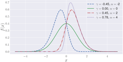
Figure 1: Skew normal distributions ($\xi=0,\omega=1$).

Figure 1 illustrates the PDFs of the skew normal distribution with fixed location parameter $\xi=0$ and scale parameter $\omega=1$, but with different shape parameters, i.e., $\alpha=-2,0,2,4$. From the figure, we observe that a larger $\alpha$ yields a larger skewness value $\gamma$. Moreover, with fixed $\xi$ and $\omega$, it is clear that enlarging $\alpha$ increases the probability $p(x>0)$; this argument will be later elaborated in our method and linked to the metric AUC in Section 3.3.

3 Skewness Ranking Optimization (Skew-OPT)

In this section, we first make some observations about the representations learned from BPR, based on which we briefly explain the motivation for our work, in Section 3.1. Second, we provide a detailed derivation of the proposed optimization criterion in Section 3.2; finally Section 3.3 gives the analogies between our criterion and the AUC evaluation metric.

3.1 Observation and Motivation

Most prior art for personalized ranking, such BPR [11] and WARP [14], seeks to learn effective user and item representations for item recommendation by maximizing the posterior probability of user preferences from pairs of observed and unobserved items for each user. Among these methods, BPR, the most representative work, introduces a general prior density $p(\Theta)$ that follows a normal distribution with zero mean and variance-covariance matrix $\lambda_{\Theta}I$ to complete the Bayesian modeling approach of the personalized ranking task. Nevertheless, neither BPR itself nor its succeeding works discuss the distribution of the estimator (i.e., $\hat{x}_{uij}(\Theta)$), which is however the component most related to model performance. Figure 2 plots the distribution constructed by the learned estimates for $\hat{x}_{uij}(\Theta)$ with the use of BPR training on each of the three listed datasets. From the figure, we observe that the three distributions are unimodal in general and typically skewed—the distributions for Epinions-Extend and Last.fm-360K are right-skewed with positive sample skewness values ($\hat{\gamma}=1.09$ and $\hat{\gamma}=0.373$ in panel (a) and (b), respectively), and that for Amazon-Book is almost symmetric with a close-to-zero positive skewness value ($\hat{\gamma}=0.08$ in panel (c)).

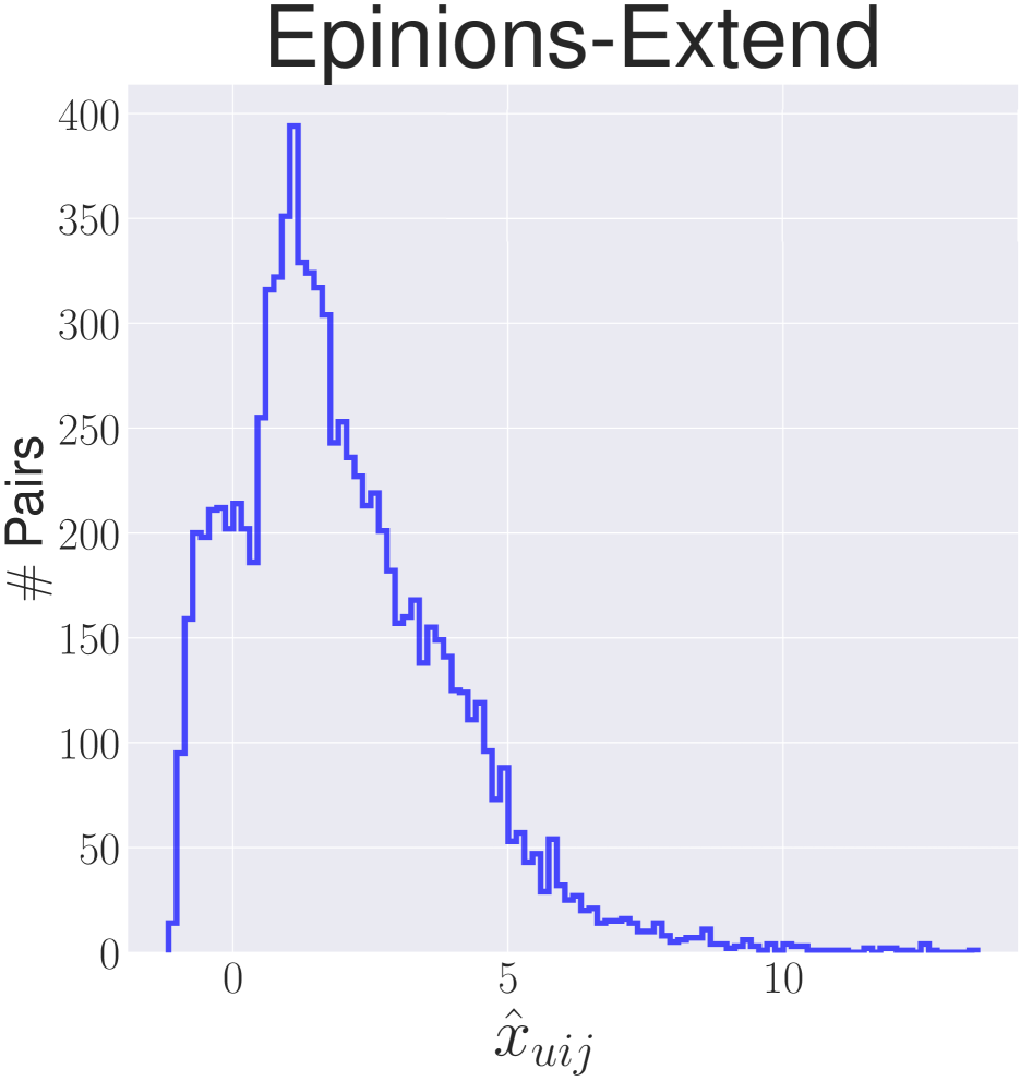
(a) $\hat{\gamma}=1.09$

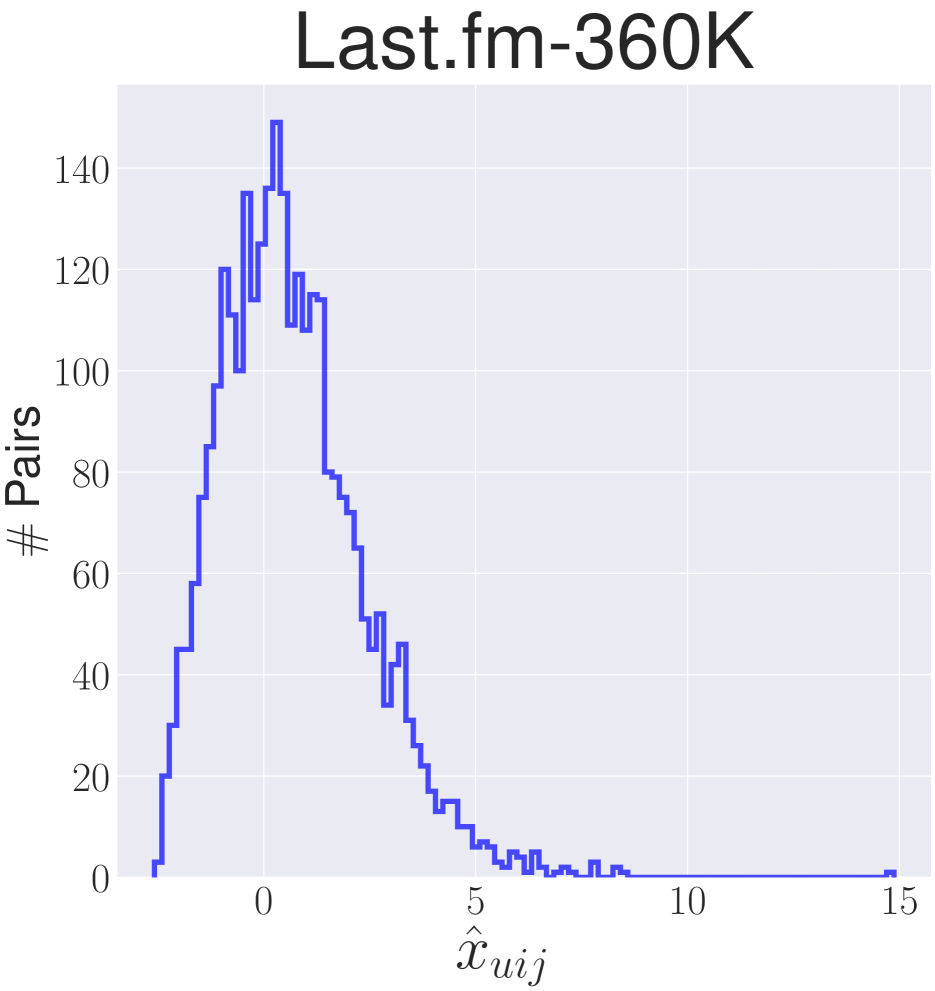
(b) $\hat{\gamma}=0.373$

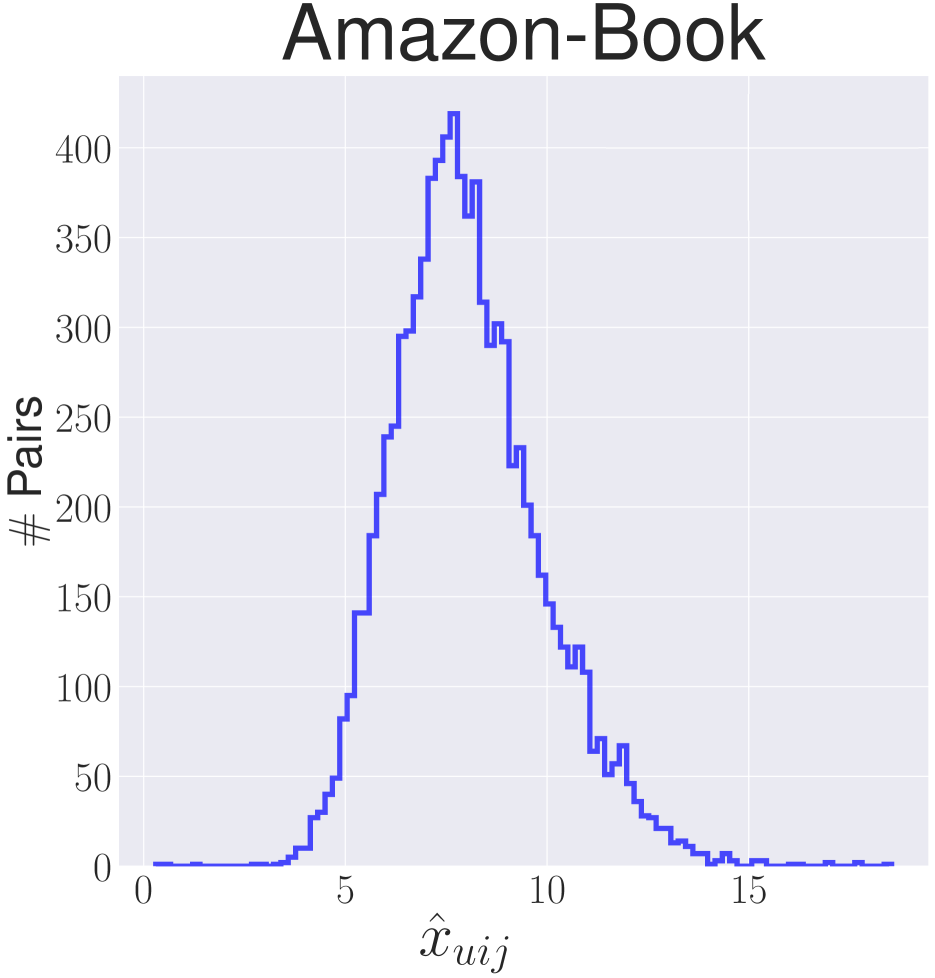
(c) $\hat{\gamma}=0.08$

Figure 2: Distributions of $\hat{x}_{uij}$ learned from BPR.

Inspired by the above observations (e.g., unimodal and skewed distributions), in this paper, we propose a simple yet novel optimization criterion that leverages features of the skew normal distribution to better model the problem. First, the location parameter $\xi$ in the skewness normal distribution provides an additional degree of freedom to allow us push the distribution of the estimator to the right; also, the scale parameter $\omega$ is used to reduce model over-fitting for large $\xi$. In addition, from Figure 1, with a fixed $\xi$ and $\omega$, enlarging the shape parameter $\alpha$ increases the probability $p(x>0)$. Here, for personalized ranking, the random variable $X$ can be used to describe the estimator $\hat{x}_{uij}$; thus, in this case, a larger $\alpha$ entails a larger probability $p(\hat{x}_{uij}>0)$, which should benefit recommendation performance. Details for the proposed optimization criterion and its link to the AUC are provided in Sections 3.2 and 3.3, respectively.

3.2 Criterion and Optimization

Motivated by the above observations as well as the properties of the skew normal distribution, in this paper we propose an unconventional optimization criterion termed skewness ranking optimization (Skew-OPT) for personalized recommendation. To this end, we recast the likelihood function referring to the individual probability that a user really prefers item $i$ to item $j$ in Eq. (2.2.1) as

$$p(i>_{u}j\,|\Theta,(\xi,\omega,\eta))=\sigma\left(\left(\frac{{\hat{x}}_{uij}(\Theta)-\xi}{\omega}\right)^{\eta}\right),$$ (5)

where $(\xi,\omega,\eta)$ denote three hyperparameters in the proposed Skew-OPT, $\eta\in\mathbb{O}$, and $\sigma(\cdot)$ denotes the sigmoid function. Above, the inclusion of $\xi$ and $\omega$ is motivated by the location and scale parameters in the skew normal distribution, respectively (see Section 2.2.3), and $\mathbb{O}$ denotes the set of positive odd integers. Note that forcing $\eta$ to be a positive odd integer ensures the rationality of the likelihood function, as under this setting it is an increasing function with argument ${\hat{x}}_{uij}$ (i.e., the distance between an observed item and a non-observed one). As mentioned previously, the location parameter $\xi$ here provides an additional degree of freedom to allow us push the distribution of the estimator to the right, and the scale parameter $\omega$ can be used to reduce overfitting for large $\xi$. It is also worth mentioning that the likelihood of BPR is a special case of Eq. (5) with $\xi=0,\omega=1,\eta=1$.

With the above likelihood function in Eq. (5), the optimization criterion becomes maximizing

Skew-OPT

$$:= \ln\prod_{(u,i,j)\in D_{S}}p\left(i>_{u}j|\Theta,(\xi,\omega,\eta)\right)\,p(\Theta)$$

$$= \sum_{(u,i,j)\in D_{S}}\ln p\left(i>_{u}j|\Theta,(\xi,\omega,\eta)\right)+\ln p(\Theta)$$

$$= \sum_{(u,i,j)\in D_{S}}\ln\sigma\left(\left(\frac{{\hat{x}}_{uij}(\Theta)-\xi}{\omega}\right)^{\eta}\right)-\lambda_{\Theta}\|\Theta\|^{2}.$$ (6)

Now, we discuss the relationship between Skew-OPT optimization and the shape parameter $\alpha$ and the corresponding skewness value.

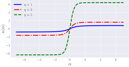
Figure 3: Increasing function $\kappa(\alpha)$ ($\xi=0,\omega=1$).

Lemma 1.

Given the case that $\hat{x}_{uij}$ follows a skew normal distribution with fixed location parameter $\xi$ and scale parameter $\omega$, maximizing the first term of Eq. (6) for a certain $\eta$ simultaneously maximizes the shape parameter $\alpha$ and the skewness value of the estimator, $\hat{x}_{uij}(\Theta)$.

Proof.

In Eq. (6), the first term can be written as

$$\sum_{(u,i,j)\in D_{S}}-\ln\left(1+e^{-\left(\frac{{\hat{x}}_{uij}(\Theta)-\xi}{\omega}\right)^{\eta}}\right).$$

Omitting the $1$ in the above equation makes it clear that maximizing the above summation is equivalent to maximizing

$$\sum_{(u,i,j)\in D_{S}}\left(\frac{{\hat{x}}_{uij}(\Theta)-\xi}{\omega}\right)^{\eta}$$

$$\propto\mathbb{E}_{(u,i,j)\sim D_{S}}\left[\left(\frac{{\hat{x}}_{uij}(\Theta)-\xi}{\omega}\right)^{\eta}\right].$$ (7)

With fixed $\xi$, $\omega$, and $\eta$, when $\hat{x}_{uij}$ follows a skew normal distribution, Eq. (7) can be represented as a function of the shape parameter $\alpha$ as

$$\kappa(\alpha) =\mathbb{E}\left[\left(\frac{{\hat{x}}_{uij}(\Theta)-\xi}{\omega}\right)^{\eta}\right],$$ (8)

Now, we prove that both $\kappa(\alpha)$ in Eq. (8) and $\gamma(\alpha)$ in Eq. (4) are increasing functions by showing that $\partial\kappa(\alpha)/\partial\alpha>0$ and $\partial\gamma(\alpha)/\partial\alpha>0$. For the former, we have

$$\partial\kappa(\alpha)/\partial\alpha$$

$$= \partial\left(\int_{-\infty}^{\infty}\left(\frac{x-\xi}{\omega}\right)^{\eta}f(x)dx\right)/\partial\alpha$$

$$= \int_{-\infty}^{\infty}\left(\frac{x-\xi}{\omega}\right)^{\eta}\partial f(x)/\partial\alpha\,dx$$

$$= \int_{-\infty}^{\infty}\left(\frac{x-\xi}{\omega}\right)^{\eta+1}\left(\frac{2}{\omega}\right)\phi\left(\frac{x-\xi}{\omega}\right)\left(\frac{e^{-\frac{\alpha^{2}\left(x-\xi\right)^{2}}{2\omega^{2}}}}{\sqrt{2\pi}}\right)dx.$$ (9)

where the density function $f(x)$ is defined in Eq. (2).

Above, the first component in Eq. (9) is greater than or equal to zero as $\eta+1$ is an even integer; the remaining three components are all positive as $\omega>0$, $\phi(\cdot)$ is a PDF, and the numerator of the last component is an exponential function. Moreover, since Eq. (9) involves integration over all $x$, it is clear that we have $\partial\kappa(\alpha)/\partial\alpha>0$, and thus $\kappa(\alpha)$ is an increasing function (see Figure 3 for example). Similarly, it is easy to prove that $\partial\gamma(\alpha)/\partial\alpha>0$, an illustration for which is shown in Figure 4. As a result, a larger expected value in Eq. (8) corresponds to a larger $\alpha$; also, the value of skewness $\gamma$ increases as $\alpha$ increases, suggesting that maximizing the first term in Eq. (6) happens to simultaneously maximize the shape parameter $\alpha$ along with the skewness of the estimator, $\hat{x}_{uij}(\Theta)$. ∎

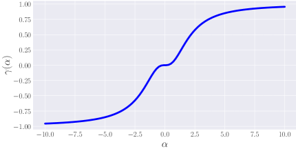
Figure 4: Increasing function $\gamma(\alpha)$.

In the optimization stage, the objective function is maximized by utilizing the asynchronous stochastic gradient ascent—the opposite of asynchronous stochastic gradient descent (ASGD) [9]—for updating the parameters $\Theta$ in parallel. For each triple $(u,i,j)\in D_{S}$, an update with learning rate $\beta$ is performed as follows (see Algorithm 1):

$$\Theta\xleftarrow{}\Theta+\beta\bigg{(}\frac{\partial\text{Skew-OPT}}{\partial\Theta}\bigg{)},$$

where the gradient of Skew-OPT with respect to the model parameters is

$$\frac{\partial\text{Skew-OPT}}{\partial\Theta}$$

$$= \sum_{(u,i,j)\in D_{S}}\frac{\partial}{\partial\Theta}\ln\sigma\left(\left(\frac{{\hat{x}}_{uij}(\Theta)-\xi}{\omega}\right)^{\eta}\right)-\lambda_{\Theta}\|\Theta\|^{2}$$

$$\propto \sum_{(u,i,j)\in D_{S}}\frac{e^{-\left(\frac{{\hat{x}}_{uij}(\Theta)-\xi}{\omega}\right)^{\eta}}}{1+e^{-\left(\frac{{\hat{x}}_{uij}(\Theta)-\xi}{\omega}\right)^{\eta}}}\frac{\partial}{\partial\Theta}\left(\frac{\hat{x}_{uij}-\xi}{\omega}\right)^{\eta}-\lambda_{\Theta}\Theta.$$

Input $D_{S}$;

begin

       Initialize $\Theta$;

       repeat

             Sample a triple $(u,i,j)$ from $D_{S}$;

             $\Theta\xleftarrow{}\Theta+\beta\bigg{(}\frac{\partial\text{Skew-OPT}\big{(}\hat{x}_{uij}(\Theta)\big{)}}{\partial\Theta}\bigg{)}$;

      until convergence;

      return ${\Theta}$;

      

end

Algorithm 1 Model learning with Skew-OPT

3.3 Analogies to AUC optimization

With our optimization formulation in Section 3.2, we here analyze the relationship between Skew-OPT and AUC. The AUC per user is commonly defined as

$${{\rm AUC}(u)}:=\frac{1}{\left|I_{u}^{+}\right|\left|I\setminus I_{u}^{+}\right|}\sum_{i\in I_{u}^{+}}\sum_{j\in I\setminus I_{u}^{+}}\delta(\hat{x}_{uij}>0).$$

Above, $\delta(x_{uij})$ is the indicator function defined as

$$\delta(\hat{x}_{uij})=\begin{cases}\;1,\;\text{if}\;\;\hat{x}_{uij}>0\\ \;0,\;\text{otherwise}.\\ \end{cases}$$

The average AUC of all users is

$${\rm AUC}:= \frac{1}{\left|U\right|}\sum_{u\in U}{{\rm AUC}(u)}$$

$$= \sum_{(u,i,j)\in D_{S}}w_{u}\delta(\hat{x}_{uij}>0),$$ (10)

where

$$w_{u}=\frac{1}{\left|U\right|\left|I_{u}^{+}\right|\left|I\setminus I_{u}^{+}\right|}.$$

The analogy between Eq. (10) and the objective function of BPR is clear as their main difference is the normalizing constant. Note that BPR is a special case with $\xi=0,\omega=1,\eta=1$ in the proposed Skew-OPT. With Skew-OPT, the analogy becomes a bit involved and is explained as follows. In the proposed Skew-OPT with fixed hyperparameters $\xi,\omega,\eta$, Lemma 1 states that maximizing the first term of Eq. (6) simultaneously maximizes the shape parameter $\alpha$ under the assumption of the skew normal distribution for the estimator. Moreover, as mentioned in Sections 2.2.3 and 3.1, it is clear that increasing $\alpha$ enlarges the probability $p(\hat{x}_{uij}>0)$, which is equal to the area under the PDF curve for $\hat{x}_{uij}>0$. This characteristic hence clearly shows the analogy between Eq. (10) and Skew-OPT.

Whereas the AUC above refers to the macro average of the AUC values for all users, we here consider the micro average version defined as

$${\rm AUC}^{\rm micro}:=\frac{1}{|D_{S}|}\sum_{(u,i,j)\in D_{S}}\delta(\hat{x}_{uij}>0).$$ (11)

Under the assumption that $\hat{x}_{uij}$ follows the skew normal distribution with fixed location parameter $\xi$ and scale parameter $\omega$, Eq. (11) can be rewritten as

$${\rm AUC}^{\rm micro}:= \mathbb{E}\,[\delta(\hat{x}_{uij}>0)\,]=p(\hat{x}_{uij}>0)$$

$$= 1-F(0)$$

$$= 1-\Psi\left(\frac{0-\xi}{\omega}\right)+2T\left(\left(\frac{0-\xi}{\omega}\right),\alpha\right),$$

where $F(x)$ is the CDF of the skew normal distribution defined in Eq. (3). Additionally, when $\alpha\rightarrow\infty$, AUC^micro achieves its maximum value, one, with $\xi\geq 0$, because

$$\forall\xi\geq 0,\,\, \lim_{\alpha\rightarrow\infty}2T\left(\left(\frac{0-\xi}{\omega}\right),\alpha\right)$$

$$=\frac{1}{2}\left(1+{\rm erf}\left(\frac{0-\xi}{\omega}\right)/\sqrt{2}\right)$$ (12)

$$=\Psi\left(\frac{0-\xi}{\omega}\right).$$

Note that for $\xi<0$, the limit value in Eq. (12) becomes $\frac{1}{2}\left(1-{\rm erf}\left(\frac{0-\xi}{\omega}\right)/\sqrt{2}\right)$, but in this paper we do not consider this case as we seek to maximize the estimator by shifting the distribution to the right on the horizontal axis.

4 Experiments

4.1 Dataset

To examine the performance of the proposed method, we conducted experiments on five real-world datasets with different sizes, densities, and domains, the statistics ow which are shown in Table 1. For each of the datasets, we converted the user-item interactions into implicit feedback. For the 5-star rating datasets, we treated ratings higher than or equal to 3.5 as positive feedback and the rest as negative feedback; as for the count-based datasets, we took counts higher than 3 as positive feedback and the remaining ones as negative feedback; for the CiteUlike dataset, since it is already composed of binary user preferences, no transformation was needed.

	Users	Items	Edges	Edge type
CiteULike	5,551	16,980	210,504	like/dislike
Amazon-Book	70,679	24,916	846,522	5-star
Last.fm-360K	23,566	48,123	303,4763	play count
MovieLens-Latest	259,137	40,110	24,404,096	5-star
Epinions-Extend	701,498	110,235	12,581,748	5-star

Table 1: Dataset statistics

CiteUlike Amazon-Book Last.fm-360K MovieLens-Latest Epinions-Extend Recall@10 mAP@10 Recall@10 mAP@10 Recall@10 mAP@10 Recall@10 mAP@10 Recall@10 mAP@10 WRMF [10, 4] 0.2159 0.1236 0.0950 0.0374 0.1308 0.0576 0.2122 0.1061 0.1025 0.0415 BPR [11] 0.2217 0.1332 0.0972 0.0390 0.1394 0.0690 0.1952 0.1097 0.1137 0.0584 WARP [14] 0.1859 0.1033 0.0869 0.0356 $\dagger$ 0.1763 $\dagger$ 0.0937 $\dagger$ 0.2748 $\dagger$ 0.1634 0.1479 0.0711 Hop-Rec [16] 0.2232 0.1319 $\dagger$ 0.1072 $\dagger$ 0.0426 0.1701 0.0870 0.2557 0.1419 $\dagger$ 0.1617 $\dagger$ 0.0813 NGCF [13] $\dagger$ 0.2321 $\dagger$ 0.1367 0.0818 0.0335 - - - - - - Skew-OPT ($\eta=1$) *0.2413 *0.1541 0.1069 *0.0467 *0.1976 *0.1051 0.2809 0.1636 *0.1743 *0.0914 Improv. ($\%$) +3.96% +12.72% -0.27% +9.62% +12.08% +12.17% +2.21% +0.12% +7.79% +12.42% Skew-OPT ($\eta=3$) *0.2481 *0.1591 *0.1173 *0.0504 *0.2032 *0.1103 *0.2852 *0.1686 *0.1768 *0.0941 Improv. ($\%$) +6.89% +16.38% +9.42% +18.07% +15.25% +17.71% +3.78% +3.18% +9.33% +15.74% Skew-OPT ($\eta=5$) *0.2553 *0.1626 *0.1163 *0.0522 *0.2012 *0.1083 *0.2879 *0.1699 *0.1758 *0.0915 Improv. ($\%$) +9.91% +18.94% +8.48% +22.53% +14.12% +15.58% +4.76% +3.97% +8.71% +12.54%

Table 2: Recommendation performance. The † symbol indicates the best performing score among all the compared models; ‘*’ and ‘Improv. (%)’ denote statistical significance at $p\text{-value}<0.01$ with a paired t-test and the percentage improvement of the proposed model, respectively, with respect to the best performing value in the baselines.

4.2 Baseline Algorithms

In the following experiments, we compared our proposed model with the following five representative and widely used recommendation algorithms.

• WRMF [10, 4] (weighted regularized matrix factorization) a relational weighted version of matrix factorization optimized by utilizing least-square learning with an addition regularization term.

• BPR [11] (Bayesian personalized ranking) adopts pairwise ranking loss for personalized recommendation and exploits direct user-item interactions to separate negative items from positive items.

• WAPR [14] (weighted approximate-rank pairwise) an improved ranking-based embedding model based on BPR, which weighs pairwise violations depending on their position in the ranked list.

• Hop-Rec [16] (high-order proximity recommendation) a state-of-the-art hybrid model that integrates the concepts of graph-based and factorization-based models, where high-order neighbors in a user-item interaction graph are exploited to enrich the information.

• NGCF [13] (neural graph collaborative filtering) the state-of-the-art neural-based CF model that recursively propagates the embeddings on the user-item interaction graph, where high-order connectivity is also encoded into user and item embeddings.

4.3 Evaluation and Settings

In the experiments, we focus on top-$N$ item recommendation. To evaluate the model capability for this task, we utilized the following two commonly used performance evaluation metrics: 1) recall and 2) mean average precision (mAP). For all datasets, we randomly divided the interaction data into 80$\%$ and 20$\%$ as the training set and the testing set, respectively. Also, the reported results are the averaged results over five repetitions in this manner. In addition, the dimensions of embedding vectors were all fixed to 128, and all the hyperparameters of compared models were determined via a grid search over different settings, from which the combination that leads to the best performance was chosen. The ranges of hyperparameters we searched for the compared methods are listed as follows.

4.4 Experimental Results

In the following sections, we demonstrate the recommendation performance and several characteristics of the proposed Skew-OPT. First, we conduct the experiments on the task of top-$N$ recommendation and compare the proposed method with the five baselines. We then provide a sensitivity analysis for the three key hyperparameters in our model. Finally, we study the learned distributions of the estimator for the five datasets and compare them with the skew normal distribution.

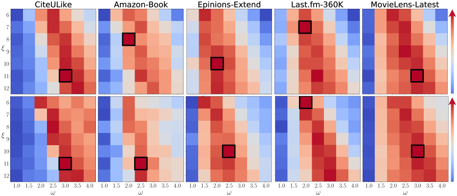
Figure 5: Sensitivity analysis. The first and the second rows represent the results for $\eta=3$ and $\eta=5$, respectively.

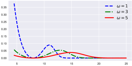
Figure 6: Gradient smoothing ($\xi=8$, $\eta=3$).

4.4.1 Top-$N$ Recommendation Performance

Table 2 compares the top-$N$ recommendation performance of Skew-OPT and the five baseline methods, where we list the results with $\eta=1,3,5$ for comparison; the best results are highlighted in bold. For NGCF, we report only the results on Amazon-book and CiteULike due to computational resource limitations. Note that the $\dagger$ symbol in the table indicates the best performing method among all the baseline methods, and the reported percentage improvement (Improv. (%)) denotes the improvement of the proposed Skew-OPT with respect to the best-performing baseline. Observe from the table that WARP, HOP-rec, and NGCF serve as strong and competitive baselines. Even so, the proposed Skew-OPT surpasses all five baselines by a significant amount for the experiments on all five datasets. The results demonstrate that the proposed model maintains consistent superior performance among different datasets in terms of both recall@10 and mAP@10, where the improvements range from 3.78% to 15.25% in Recall@10 and from 3.18% to 18.07% in mAP@10 when $\eta=3$, and from 4.76% to 14.12% in Recall@10 and from 3.97% to 22.53% in mAP@10 when $\eta=5$. Hence, according to the results reported in Table 2, we believe such improvements are substantial, thereby significantly advancing the existing state of the art. It is also worth mentioning that the proposed Skew-OPT achieves better results than Hop-Rec and NGCF by solely using user-item interactions without exploring high-order connections.

4.4.2 Sensitivity Analysis

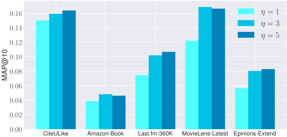
(a) $\xi=11$, $\omega=3$

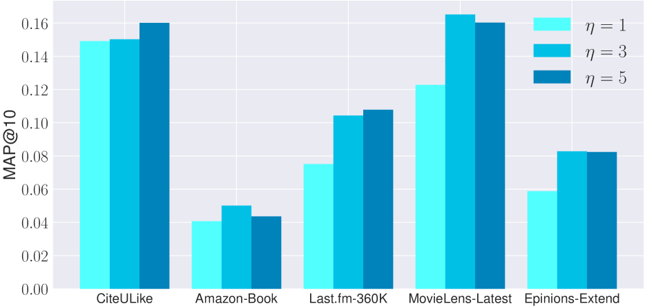
(b) $\xi=12$, $\omega=3$

Figure 7: Sensitivity analysis on $\eta$.

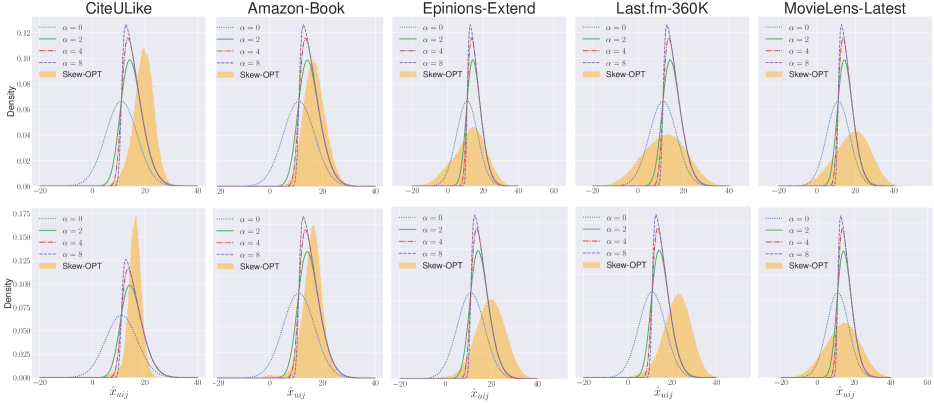
Figure 8: Learned distributions and the skew normal distributions ($\xi=11$, $\omega=3$). The first and the second rows represent the distributions when $\eta=3$ and $\eta=5$, respectively. The bar plots in red denotes the learned distributions with Skew-OPT, and the curves corresponds to the skew normal distributions with $\xi=11$ and $\omega=3$ but with various values of shape parameter $\alpha$.

Figure 5 shows the heat maps for mAP@10 on the two key hyperparameters $\xi$ and $\omega$ in the proposed Skew-OPT; note that we here plot the results only for $\eta=3,5$ as these two values yield consistently better performance than $\eta=1$ as shown in Table 2. From the figure, we observe that increasing $\xi$, which stands for the location parameter of the estimator, generally improves the performance while considering a proper $\omega$. In addition, the results of all of the five datasets display a similar tendency in this sensitivity check; that is, a large $\xi$ usually requires a large $\omega$ and a small $\xi$ considers a small $\omega$. In other words, if we consider the parameter setting in an opposite direction from this characteristic, the performance of our model deteriorates. This is due to the fact that increasing $\xi$ actually increases the possibility of the model overfitting whereas a large $\omega$ yields gradient smoothing for the optimization (see Figure 6 which demonstrates the gradient smoothing effect), thereby better balancing the overfitting that results from a large $\xi$. Note that the square framed in black in each of the sub-figures of Figure 5 denotes the best performance for each dataset, the value of which is listed in Table 2 (see the values in the columns for mAP@10 in the table). We also provide sensitivity checks on $\eta=1,3,5$ with fixed $\xi=11$ and $\omega=3$ and $\xi=12$ and $\omega=3$ in Figure 7. The figure shows that under the same location parameter and scale parameter, $\eta=3$ and $\eta=5$ usually yield better performance than $\eta=1$ among all datasets.

4.4.3 Distribution Analysis

Figure 8 compares the learned distribution of the estimator $\hat{x}_{uij}$ for each dataset to the corresponding skew normal distribution under the setting of $\xi=11$ and $\omega=3$. Note that the learned distribution is generated from the training data with the model trained on the hyperparameters same as the above setting, i.e., $\xi=11,\omega=3$, and $\eta=3$ (the first row) or $\eta=5$ (the second row). From the figure, we observe that the learned distributions are with similar shapes to the right-skewed normal distributions, especially under the case that $\eta=5$. It is worth noting that as Skew-OPT does not directly constrain the distribution, there is by nature no guarantee on the shape of the learned distributions. Moreover, except for the maximization to the likelihood function in the objective function (i.e., the first term in the objective), Skew-OPT also involves a regularization term; as a result, it is nature that the learned distributions do not exactly fit the skew normal distributions with the same $\xi$ and $\omega$. Even so, from Figure 8, we observe that the learned distributions for all datasets are all right-skewed, which corresponds to the statement in Lemma 1 and the AUC analogies in Section 3.3. On the other hand, Figure 9 shows the learned distributions when adopting different location parameters $\xi$ but with fixed $\omega=2$ and $\eta=3$. As shown in the figure, pushing $\xi$ to be a larger value indeed moves the distribution to the right, thereby increasing the possibility of $\hat{x}_{uij}>0$ and thus the potential to boost the recommendation performance.

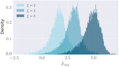
Figure 9: Learned distributions with different location parameters ($\omega=2$ and $\eta=3$).

5 Conclusions

This paper proposes an unconventional optimization criterion, Skew-Opt, that leverages features of the skew normal distribution to better model the problem of personalized recommendation. Specifically, the developed criterion is parameterized with three hyperparameters, thereby providing additional degrees of freedom for ranking optimization. We further present theoretical insights on the relation between the maximization of Skew-OPT and the shape parameter in the skew normal distribution along with the skewness as well as the asymptotic results of the criterion to AUC maximization. Experimental results show that models trained with the proposed Skew-OPT yield consistently the best recommendation performance on all tested datasets. In addition, the sensitivity and distribution analyses not only provide valuable and practical insights for choosing the hyperparameters but also attest the importance of the characteristics of the learned distribution to the recommendation performance. In sum, this work is the first that explicitly considers the distribution of the estimator for recommendation algorithms; exploring the way to shape the estimator distribution should be of great potential to boost recommendation performance and is an interesting future research direction worth to further investigate.

References

- [1] Chen, C.-M., Wang, C.-J., Tsai, M.-F., and Yang, Y.-H. Collaborative similarity embedding for recommender systems. In Proceedings of the 28th International Conference on World Wide Web, WWW ’19, Association for Computing Machinery, p. 2637–2643.
- [2] He, R., Kang, W.-C., and McAuley, J. Translation-based recommendation. In Proceedings of the 11th ACM Conference on Recommender Systems, RecSys ’17, Association for Computing Machinery, p. 161–169.
- [3] Hsieh, C.-K., Yang, L., Cui, Y., Lin, T.-Y., Belongie, S., and Estrin, D. Collaborative metric learning. In Proceedings of the 26th International Conference on World Wide Web, WWW ’17, International World Wide Web Conferences Steering Committee, p. 193–201.
- [4] Hu, Y., Koren, Y., and Volinsky, C. Collaborative filtering for implicit feedback datasets. In Proceedings of the 8th IEEE International Conference on Data Mining, ICDM ’08, IEEE Computer Society, p. 263–272.
- [5] Kabbur, S., Ning, X., and Karypis, G. Fism: Factored item similarity models for top-n recommender systems. In Proceedings of the 19th ACM SIGKDD International Conference on Knowledge Discovery and Data Mining, KDD ’13, Association for Computing Machinery, p. 659–667.
- [6] Koren, Y., Bell, R., and Volinsky, C. Matrix factorization techniques for recommender systems. Computer 42, 8, 30–37.
- [7] Liang, D., Altosaar, J., Charlin, L., and Blei, D. M. Factorization meets the item embedding: Regularizing matrix factorization with item co-occurrence. In Proceedings of the 10th ACM Conference on Recommender Systems, RecSys ’16, Association for Computing Machinery, p. 59–66.
- [8] Ning, X., and Karypis, G. Slim: Sparse linear methods for top-n recommender systems. In Proceedings of the 11th IEEE International Conference on Data Mining, ICDM ’11, IEEE Computer Society, p. 497–506.
- [9] Niu, F., Recht, B., Re, C., and Wright, S. J. Hogwild! a lock-free approach to parallelizing stochastic gradient descent. In Proceedings of the 24th International Conference on Neural Information Processing Systems, NIPS’11, Curran Associates Inc., p. 693–701.
- [10] Pan, R., Zhou, Y., Cao, B., Liu, N. N., Lukose, R., Scholz, M., and Yang, Q. One-class collaborative filtering. In Proceedings of the 8th IEEE International Conference on Data Mining, ICDM ’08, IEEE Computer Society, p. 502–511.
- [11] Rendle, S., Freudenthaler, C., Gantner, Z., and Schmidt-Thieme, L. Bpr: Bayesian personalized ranking from implicit feedback. In Proceedings of the 25th Conference on Uncertainty in Artificial Intelligence, UAI ’09, AUAI Press, p. 452–461.
- [12] Wang, X., He, X., Cao, Y., Liu, M., and Chua, T.-S. Kgat: Knowledge graph attention network for recommendation. In Proceedings of the 25th ACM SIGKDD International Conference on Knowledge Discovery and Data Mining, KDD ’19, Association for Computing Machinery, p. 950–958.
- [13] Wang, X., He, X., Wang, M., Feng, F., and Chua, T.-S. Neural graph collaborative filtering. In Proceedings of the 42nd International ACM SIGIR Conference on Research and Development in Information Retrieval, SIGIR’19, Association for Computing Machinery, p. 165–174.
- [14] Weston, J., Bengio, S., and Usunier, N. Wsabie: Scaling up to large vocabulary image annotation. In Proceedings of the 22nd International Joint Conference on Artificial Intelligence, IJCAI’11, AAAI Press, p. 2764–2770.
- [15] Weston, J., Yee, H., and Weiss, R. J. Learning to rank recommendations with the k-order statistic loss. In Proceedings of the 7th ACM Conference on Recommender Systems, RecSys ’13, Association for Computing Machinery, p. 245–248.
- [16] Yang, J.-H., Chen, C.-M., Wang, C.-J., and Tsai, M.-F. Hop-rec: High-order proximity for implicit recommendation. In Proceedings of the 12nd ACM Conference on Recommender Systems, RecSys ’18, Association for Computing Machinery, p. 140–144.