Dispersion measure components within host galaxies of Fast Radio Bursts: observational constraints from statistical properties of FRBs

Abstract

Dispersion measure (DM) of Fast Radio Bursts (FRBs) are commonly used as a indicator of distance assuming that DM in excess of the expected amount within the Milky Way in the direction of each FRB arise mostly from the inter-galactic medium. However, the assumption might not be true if, for example, most FRB progenitors are embedded in ionized circumstellar material (CSM, e.g. supernova remnant). In this study, we jointly analyze distributions of DM, flux density, and fluence of the FRB samples observed by the Parkes telescope and the Australian Square Kilometre Array Pathfinder (ASKAP) using analytical models of FRBs, to constrain fractions of various DM components that shape the overall DM distribution and emission properties of FRBs. Comparing the model predictions with the observations we find that the typical amount of DM in each FRB host galaxy is $\sim 120$ cm^-3pc which is naturally explained as a combination of interstellar medium (ISM) and halo of an ordinary galaxy, without additional contribution from ionized CSM that is directly associated with an FRB progenitor. Furthermore, we also find that observed flux densities of FRBs do not statistically suffer strong $K$-correction, i.e. the typical luminosity density of FRBs does not significantly change within the range of emitting frequency $\nu_{\rm rest}\sim$ 1–4 GHz.

1 Introduction

A Fast Radio Burst (FRB) is a transient astronomical object observed at $\sim$ 1 GHz frequency with a typical duration of several milliseconds, whose origin is not yet known (e.g., Lorimer et al., 2007; Keane et al., 2012; Thornton et al., 2013). More than a hundred FRB sources have been discovered so far. Roughly 20 FRB sources are known to produce bursts repeatedly (repeating FRBs), while other FRB sources do not show any repetition (non-repeating FRBs), implying a possibility that they are different populations of astronomical objects (Palaniswamy et al., 2018).

FRBs have large dispersion measures (column density of free electrons along a line of sight which is measured with delay of pulse arrival time as a function of frequency, hereafter DMs) that exceed the expected amounts within the Milky Way (MW) in their direction. Their large DMs suggest that FRBs are extragalactic objects. Although various theoretical models have been proposed (e.g., Totani, 2013; Kashiyama et al., 2013; Popov & Postnov, 2013; Falcke & Rezzolla, 2014; Cordes & Wasserman, 2016; Zhang, 2017, see Platts et al. 2019 for a recent review), observational evidence that confirms or rejects those models is still lacking.

Most of the currently known FRBs have been discovered by widefield radio telescopes with typical localization accuracy of $\gtrsim$ 10 arcmin, and hence it is challenging to identify their counterparts or host galaxies in most of the cases (e.g., Petroff et al., 2015; DeLaunay et al., 2016; Niino et al., 2018; Tominaga et al., 2018). Currently, identifications of FRB host galaxies, and hence distance measurements that are independent of DM, have been achieved only for 5 FRBs (2 repeating and 3 non-repeating FRBs at redshifts $z\sim 0.03$–0.7, Tendulkar et al., 2017; Bannister et al., 2019; Ravi et al., 2019; Prochaska et al., 2019; Marcote et al., 2020). Distances of other FRBs are estimated from their DMs assuming that the DMs in excess of the expected MW component (${\rm DM_{EX}}$) arise mostly from the inter-galactic medium (IGM), and considered to be widely distributed over a redshift range $z\sim 0.1$–2.5. However the actual distances of FRBs can be shorter than the estimations if significant fraction of the DMs arise from other ionized gas components than the IGM.

As locations of FRBs are not known in most of the cases, statistical distributions of observed ${\rm DM_{EX}}$ and flux density (or fluence) are important clues to understand the nature of FRBs (e.g., Dolag et al., 2015; Katz, 2016; Caleb et al., 2016). Analyzing the statistical properties of FRBs discovered by the Parkes radio telescope, Niino (2018, hereafter N18) showed that the observed properties are better explained if FRBs are at cosmological distances and the cosmic FRB rate density [$\rho_{\mathrm{FRB}}(z)$] increases with redshift resembling the cosmic star formation history (CSFH), while a model in which FRBs originate in the local universe (i.e., ${\rm DM_{EX}}$ is dominated by non-IGM component) is disfavored. However, quantitative constraint on the fraction of the IGM and non-IGM components in ${\rm DM_{EX}}$ of FRBs was not obtained by the analysis in N18.

Recently, an energetic radio burst from a Galactic magnetar, SGR 1935+2154, was observed (The CHIME/FRB Collaboration, 2020; Bochenek et al., 2020). The magnetar radio burst emitted $\sim 10^{35}$ erg during its $\sim 1$ ms duration. This luminosity is comparable to $\sim$ 1/30 of the faintest extragalactic FRB ever observed (a burst from a repeating FRB 180916.J0158+65 Marcote et al., 2020), or $\sim 10^{-4}$ of typical FRBs. Whether all (or majority of) FRBs are similar phenomena to the burst from SGR 1935+2154 is still a matter of debate. It is possible to reconcile the inferred event rate of magnetar radio bursts like that from SGR 1935+2154 with the luminosity function (LF) of extragalactic FRBs (Margalit et al., 2020; Lu et al., 2020). However, Margalit et al. (2020) also pointed out that the typical distance of extragalactic FRBs would be shorter than that estimated from ${\rm DM_{EX}}$, if the FRB LF is directly connected to the inferred event rate of magnetar radio bursts in its faint-end.

Previous investigations of FRB LF have been conducted assuming that contributions of non-IGM components to ${\rm DM_{EX}}$ do not significantly exceed the amount expected from diffuse interstellar medium (ISM) of an FRB host galaxy which is usually smaller than the IGM component (N18; Luo et al., 2018, 2020; Lu & Piro, 2019). However, the assumption might not be true if most FRB progenitors are embedded in ionized circumstellar material (CSM, e.g. supernova remnant, pulsar wind nebula, HII region, see Kokubo et al., 2017; Piro & Burke-Spolaor, 2017). It is essential to unveil actual distances and luminosities of FRBs, to understand the nature of FRBs and clarify their relation to magnetar radio bursts. In this study, we jointly analyze the statistical properties of the FRB samples observed by the Parkes telescope and the Australian Square Kilometre Array Pathfinder (ASKAP), to put constraints on non-IGM DM components associated with FRB progenitors based on the observational data.

In Section 2, we describe the datasets that we use to constrain the properties of FRBs. In Section 3, we describe our model of FRB population. In Section 4, we discuss constraints on the typical luminosity of FRBs and the amount of non-IGM DM components from the ${\rm DM_{EX}}$ distributions of the observed FRB samples. In Section 5, we discuss how the constraints are affected by spectra of FRBs statistically (i.e., effects of $K$-correction). In Section 6, we discuss constraints obtained from the distribution functions of flux densities and fluences of the FRB samples. We summarize our conclusions in section 7. Throughout this paper, we assume the fiducial cosmology with $\Omega_{\Lambda}=0.7$, $\Omega_{m}=0.3$, and $H_{0}=$ 70 km s^-1 Mpc^-1.

2 FRB datasets

To constrain the properties of FRB, we use the sample of FRBs discovered by the Parkes telescope and ASKAP. The properties of the observed FRBs are collected from the FRBCAT database (Petroff et al., 2016), as reported at the beginning of September 2019. We exclude FRB180923, the last Parkes FRB before the date of data collection, from the Parkes sample because its peak flux density which we use in our analysis is not reported. We also exclude FRBs discovered by ASKAP in 2019 (FRB 190711, and 190714) from the ASKAP sample for the same reason. We note that there are four outlier FRBs in the Parkes sample compared to the overall $S_{\nu}$–DM distribution of the sample, which have extremely bright flux density and small DM, and we exclude these FRBs (FRB 010724, 110214, 150807, 180309) from our analysis. In total, the Parkes sample includes 24 FRBs between FRB 010125 and 180714, and the ASKAP sample includes 26 FRBs between FRB 170107 and 180924.

3 Models

3.1 $\rho_{\mathrm{FRB}}$ and LF

Investigating the distributions of DM and apparent flux density of FRBs discovered by the Parkes radio telescope, N18 showed that $\rho_{\mathrm{FRB}}$ increases with redshift resembling CSFH, and an LF model with a bright-end cutoff at log${}_{10}L_{\nu}$ [erg s^-1Hz^-1] $\sim$ 34 are favored to reproduce observations, while faint-end of the LF is not well constrained. The existence of the bright-end cutoff in FRB LF is also independently shown by Luo et al. (2018). In this study, we assume that $\rho_{\mathrm{FRB}}(z)$ is proportional to CSFH as derived by Madau & Dickinson (2014), and use the following LF models to examine how our results are affected by the difference of the faint end of the FRB LF (Figure 1);

• Power-law distribution function with index $\alpha$, and exponential cutoff in the bright-end above $L_{\nu,0}$ (PL+E):

  $$\frac{d\phi}{dL_{\nu}}\propto L_{\nu}^{\alpha}exp(-\frac{L_{\nu}}{L_{\nu,0}}).$$ (1)

  We consider the cases with $\alpha=-2,-1$, and 0 in this study ($\alpha=-1$ as a baseline and $\alpha=-2,0$ as steep and flat variants).

• Log-normal distribution with median $L_{\nu,0}$:

  $$\frac{d\phi}{dL_{\nu}}\propto\frac{{\rm log_{10}}e}{\sqrt{2\pi}\sigma L_{\nu}}{\rm exp}(-\frac{({\rm log_{10}}L_{\nu}-{\rm log_{10}}L_{\nu,0})^{2}}{2\sigma^{2}}).$$ (2)

  We assume $\sigma=0.5$ dex in this study.

$L_{\nu,0}$ in each LF model is a free parameter which will be constrained by comparing model predictions with observations.

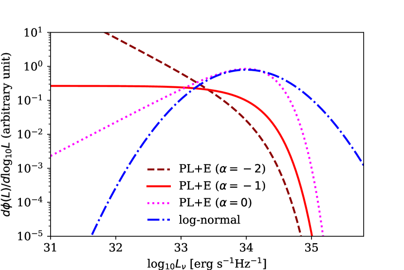
Figure 1: The LF models considered in this study. The dashed, solid, and dotted lines represent the power-law plus exponential cutoff (PL+E) models with $\alpha=-2,-1$, and 0, respectively. The dot-dashed line represents the log-normal model. $L_{\nu,0}=10^{34}$ erg s^-1Hz^-1 in this figure.

3.2 Receiver efficiency, propagation effect, and $K$-correction

It should be noted that the efficiency of the Parkes multi-beam receiver (Staveley-Smith et al., 1996) largely varies within its beam, and the reported flux densities and fluences are converted from the observed signal assuming the receiver efficiency at the beam center, and thus effectively are lower-limits.

To account for the variation of the receiver efficiency, N18 computed the probability distribution function (PDF) of receiver efficiency assuming the beam shape of the Parkes multi-beam receiver is represented by an Airy disc, and convoluted the flux density PDF of the FRB model with the receiver efficiency PDF. We follow the method of N18 when we compare our model predictions with the Parkes sample of observed FRBs. On the other hand, the ASKAP phased array feed receivers sample the focal plane almost uniformly (Bannister et al., 2017; Shannon et al., 2018), and hence we do not use the receiver efficiency PDF model when we discuss the observed properties of the ASKAP sample.

Observed flux density of an FRB is also affected by various propagation effects between the source and the observer. Scattering of an FRB signal suppress FRB flux density by pulse broadening, on the other hand, scintillation and plasma lensing may also enhance FRB flux density (e.g., Hassall et al., 2013; Cordes et al., 2016, 2017). Following N18, we treat PDF of propagation effects as included in the FRB LF rather than trying to separate intrinsic luminosity of an FRB from propagation effects.

$K$-correction is also an important effect when we consider observed flux densities of objects at cosmological distances. In this study, we consider the cace in which the $K$-correction factor $\kappa_{\nu}(z)=L_{\nu}(\nu_{\rm rest})/L_{\nu}(\nu_{\rm obs})=1$ as a baseline model in Section 4, and discuss how our the results are affected by $K$-correction in Section 5. Here $\kappa_{\nu}(z)=1$ means that the typical spectral index of FRBs is 0 in a statistical meaning (${\beta_{\rm stat}}=0$), or that the FRB LF is not changed with rest frame frequency in the range of $\nu_{\rm rest}\sim$ 1–4 GHz which is covered by the current sample, but not that most FRBs have a flat spectrum.

3.3 The detection threshold

To make model predictions of observed FRB properties, we need to determine a detection threshold for model FRBs. In N18, we considered a model FRB as detected when its flux density exceeds a threshold value, $S_{\nu}\geq S_{\nu,{\rm th}}$. Detectability of an FRB is affected not only by its flux density but also on the pulse width in reality (and hence the fluence ($F_{\nu}$), Keane & Petroff, 2015). However, N18 pointed out that signal-to-noise ratio (S/N) of FRB detections in the Parkes sample empirically correlates well with flux density, and the faint-end of the flux density distribution of the Parkes sample is sharply cut. These facts suggest that $S_{\nu}$ is effectively a good proxy for S/N. In this study, we assume the threshold flux density of $S_{\nu,{\rm th}}=0.4$ Jy and 15 Jy for the Parkes and ASKAP samples, based on the faint end of the $S_{\nu}$ distributions of the two samples which we show in Section 6.

3.4 DM computation

We consider DM of an FRB as a summation of 4 components, DM = ${\rm DM_{ISM}}+{\rm DM_{halo}}+{\rm DM_{IGM}}+{\rm DM_{host}}$, where ${\rm DM_{ISM}}$ and ${\rm DM_{halo}}$ are the DM components associated with the ISM and the halo of MW, ${\rm DM_{IGM}}$ arises from the IGM between the host galaxy of the FRB and MW, and ${\rm DM_{host}}$ arises from ionized gas within the host galaxy. We note that ${\rm DM_{host}}$ includes DM components that arise from the galaxy scale ISM, the host galaxy halo, and possible CSM that is directly associated with the progenitor of the FRB (e.g. supernova remnant, pulsar wind nebula, HII region).

In the FRBCAT database, excess of observed DM beyond ${\rm DM_{ISM}}$ (${\rm DM_{EX}}={\rm DM_{halo}}+{\rm DM_{IGM}}+{\rm DM_{host}}$) is reported for each event assuming the NE2001 model of free electrons in the Galactic ISM (Cordes & Lazio, 2002), and we compare these values to the model predictions. Some previous studies have independently shown that ${\rm DM_{halo}}$ is typically $\sim 50$ cm^-3pc (Dolag et al., 2015; Prochaska & Zheng, 2019; Yamasaki & Totani, 2020). In this study, we assume ${\rm DM_{halo}}=30$ cm^-3pc for any FRB following Dolag et al. (2015).

${\rm DM_{IGM}}$ is determined by the distance between the FRB host galaxy and MW, i.e., redshift of the FRB (e.g., Ioka, 2003; Inoue, 2004). We use the same formalism of ${\rm DM_{IGM}}$ as in N18. In the redshift range discussed in this paper, the formalism can be naively approximated as ${\rm DM_{IGM}}\sim 1000z$ cm^-3pc.

We assume ${\rm DM_{host}}$ follows a log-normal distribution with $\sigma=0.2$ dex, motivated by theoretical models of ${\rm DM_{host}}$ distribution in a disk galaxy (Xu & Han, 2015; Walker et al., 2018; Luo et al., 2018). The median value of the distribution, ${\rm DM_{host,med}}$, is a free parameter we will constrain in the following sections. We note that the ${\rm DM_{EX}}$ distributions of the Parkes and ASKAP samples can be also approximated by log-normal distributions with $\sigma=0.2$ dex, and hence if ${\rm DM_{host}}$ occupies a large fraction of observed ${\rm DM_{EX}}$, ${\rm DM_{host}}$ must follow a PDF that resembles the log-normal distribution with $\sigma=0.2$ dex to explain observations.

4 Constraining the characteristic luminosity of FRBs and the amount of DM within their host galaxies

4.1 Fitting the DM distributions without DM components associated with FRB sources

The FRB models described in Section 3 have two free parameters, $L_{\nu,0}$ and ${\rm DM_{host,med}}$, and we will constrain these parameters by comparing predicted ${\rm DM_{EX}}$ distributions with the ${\rm DM_{EX}}$ distributions of the observed samples. First, we perform ${\rm DM_{EX}}$ distribution fitting using one parameter, $L_{\nu,0}$, assuming that contribution of an FRB host galaxy to ${\rm DM_{EX}}$ is negligible.

The goodness of fit is evaluated by the Kolmogorov-Smirnov (KS) test. Figure 2 shows the KS test probability ($P_{\rm KS}$) that the observed sample can arise from the model distribution as a function of $L_{\nu,0}$, and Figure 3 shows the best-fit ${\rm DM_{EX}}$ distributions. With any of the LF models except the steep PL+E ($\alpha=-2$), the best-fit $L_{\nu,0}$ is larger for the ASKAP sample. On the other hand, $L_{\nu,0}$ is poorly constrained for the Parkes sample in the case of the steep PL+E model of LF.

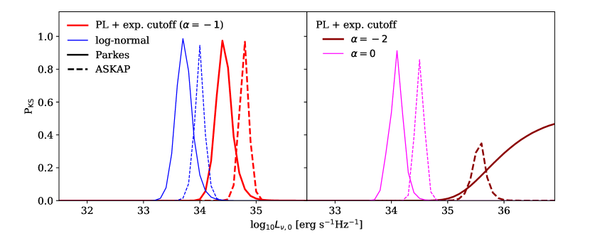
Figure 2: $P_{\rm KS}$ likelihood between the model and the observed ${\rm DM_{EX}}$ distributions as a function of $L_{\nu,0}$. The solid and dashed lines indicate the results for the Parkes and ASKAP samples, respectively. Lines with different thickness (different color in the colored version) represent results with different LM models.

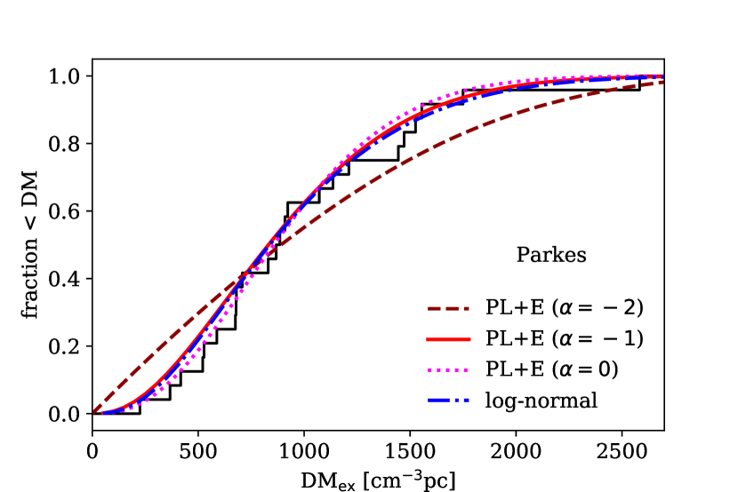
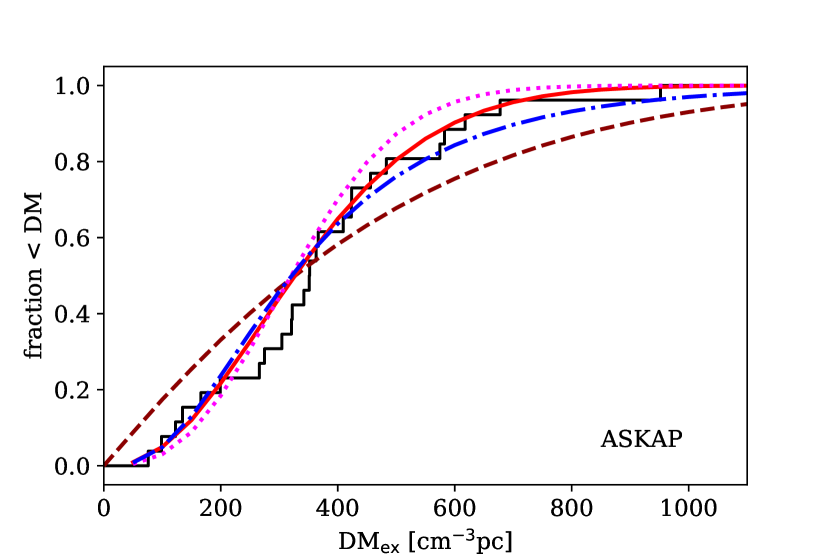
Figure 3: The cumulative ${\rm DM_{EX}}$ distributions of the observed FRB samples (histogram), and the best fit model distributions to the observations with ${\rm DM_{host}}=0$. The left and right panels shows the distributions of the Parkes and ASKAP samples, respectively. The dashed, solid, and dotted lines represent the model distributions with the PL+E LF models with $\alpha=-1.0,-2.0$, and 0.0, respectively. The dot-dashed line represents the distribution with the log-normal LF model.

4.2 Fitting the DM distributions with DM components associated with FRB sources

The observing frequencies of the Parkes telescope and ASKAP are similar to each other, and hence we consider that the best-fitting parameters that result form the fittings to the two samples should be the same. Here we perform the ${\rm DM_{EX}}$ distribution fitting using two parameters ($L_{\nu,0}$ and ${\rm DM_{host,med}}$) to find parameter sets that reproduce the ${\rm DM_{EX}}$ distributions of the two samples simultaneously.

The acceptable ranges of the parameters are shown as contours of $P_{\rm KS}$ for each of the observed samples in Figure 4. The parameter ranges that can reproduce the ${\rm DM_{EX}}$ distributions of the Parkes and ASKAP samples at a same time are also indicated ($P_{\rm KS,joint}=P_{\rm KS,Parkes}\times P_{\rm KS,ASKAP}>0.1$). The ${\rm DM_{EX}}$ distributions of the two samples can be consistently explained when ${\rm DM_{host,med}}\sim 120$ cm^-3pc, while ${\rm DM_{host,med}}\gtrsim 200$ cm^-3pc is disfavored with any of the LF models

It has been shown that contribution from ISM of a MW like host galaxy to observed DM of an FRB is $\sim 100$ cm^-3pc (Xu & Han, 2015; Walker et al., 2018; Luo et al., 2018). The predicted typical contribution of a FRB host galaxy to observed DM, ${\rm DM_{host,med}}\sim 120$ cm^-3pc, can be naturally explained as that arise from the ISM and the halo of the host galaxy, and hence suggests that a DM component that arise from CSM that is directly associated with an FRB progenitor is typically small ($<80$ cm^-3pc).

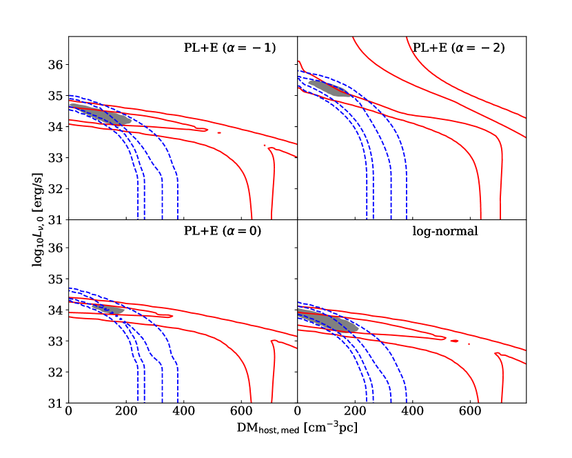
Figure 4: $P_{\rm KS}$ likelihood map on the parameter plane of ${\rm DM_{host,med}}$ and $L_{\nu,0}$. The solid and dashed contours represent $P_{\rm KS}$ (at 0.05 and 0.32) for the Parkes and ASKAP samples, respectively. Different panels show the $P_{\rm KS}$ likelihood for the four different LF models. The gray shaded regions indicates $P_{\rm KS,joint}=P_{\rm KS,Parkes}\times P_{\rm KS,ASKAP}>0.1$.

5 Effects of K-correction

In the previous section, we have assumed that $K$-correction does not affect observed flux density of an FRB [$\kappa_{\nu}(z)=1$, or ${\beta_{\rm stat}}=0$]. In this section, we examine how the results of the ${\rm DM_{EX}}$ distribution fitting changes when ${\beta_{\rm stat}}$ is changed. The acceptable ranges of the parameters with ${\beta_{\rm stat}}=1.5,-1.5$, and $-3.0$ are shown as contours of $P_{\rm KS}$ in Figure 5 for the baseline PL+E ($\alpha=-1$) and log-normal models of LF. Here the characteristic luminosity density $L_{\nu,0}$ is determined at the emitting frequency observed at $z=0$ ($\sim 1.3$ GHz in the case of the Parkes telescope and ASKAP), and the characteristic luminosity in other emitting frequency follows $\propto\nu^{\beta_{\rm stat}}$. The results with the other LF models are not qualitatively different.

The best-fitting $L_{\nu,0}$ is larger for smaller ${\beta_{\rm stat}}$ as naturally expected, and the fitting to the Parkes sample is affected more from the $K$-correction than that to the ASKAP sample, because FRBs in the Parkes sample have larger ${\rm DM_{EX}}$ (i.e., likely at higher-$z$) on average than those in the ASKAP sample. These effects make the preferred ${\rm DM_{host,med}}$ larger with larger ${\beta_{\rm stat}}$. The range of ${\rm DM_{host,med}}$ which can provide $P_{\rm KS,joint}>0.1$ depending on $L_{\nu,0}$ is shown in Figure 6 for the four LF models. In the cases of ${\beta_{\rm stat}}\leq-1.5$, there is no parameter range that reproduce the observed ${\rm DM_{EX}}$ distributions of the Parkes and ASKAP samples at a same time with the steep PL+E LF model. On the other hand, ${\rm DM_{host,med}}\gtrsim 200$ cm^-3pc is preferred when ${\beta_{\rm stat}}=1.5$, suggesting existence of other significant DM components than ISM and halo gas in FRB host galaxies.

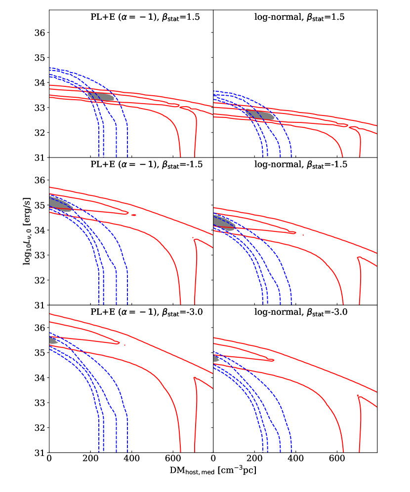
Figure 5: Same as Figure 4, but with ${\beta_{\rm stat}}=1.5$, -1.5, and -3.0 (top, middle, and bottom panels). $P_{\rm KS}$ likelihood for the baseline PL+E and log-normal models of LF are shown in the left and right panels, respectively.

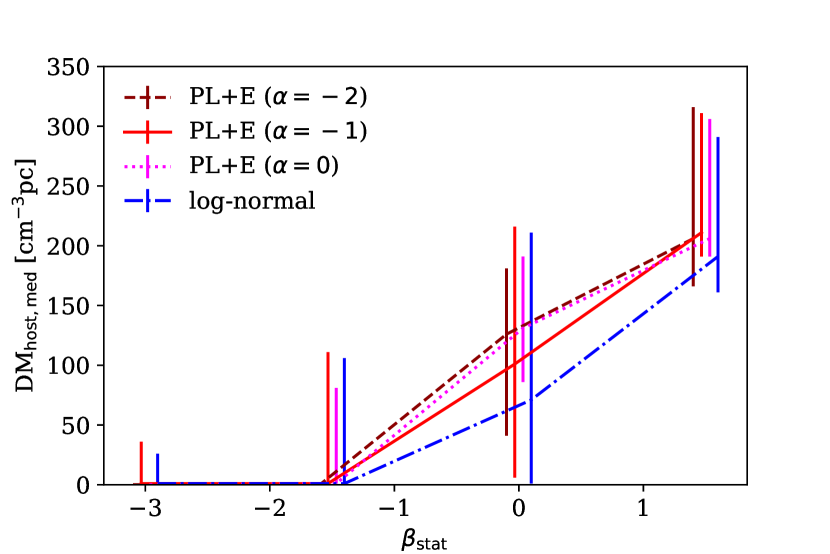
Figure 6: Possible range of ${\rm DM_{host,med}}$ that can simultaneously reproduce the observed DM distributions of the Parkes and ASKAP samples ($P_{\rm KS,joint}>0.1$) as a function of spectral index ${\beta_{\rm stat}}$. The datapoints connected with dashed, solid, dotted, and dot-dashed lines represent the results with the PL+E ($\alpha=-2.0,-1.0$, 0.0), and log-normal models of LF, respectively. The data points are slightly shifted sideways for visibility.

6 Distributions of flux density and fluence

We have seen that preferred amount of ${\rm DM_{host,med}}$ is dependent on ${\beta_{\rm stat}}$. In this section, we investigate $S_{\nu}$ (and $F_{\nu}$) distribution, so-called log$N$–log$S$ distribution, of FRBs to constrain ${\beta_{\rm stat}}$. It is widely known that $S_{\nu}$ and $F_{\nu}$ of a population of light sources follow a power-law distribution $N(>\mathcal{F})\propto\mathcal{F}^{\gamma}$ with index $\gamma=-1.5$ ($\mathcal{F}=S_{\nu}$ or $F_{\nu}$) when the light sources are homogeneously distributed in a Euclidean space, while cosmological effects can modify those distributions. As discussed in N18, the cosmological effects modify distributions of $S_{\nu}$ and $F_{\nu}$ differently. Hence we investigate both $S_{\nu}$ and $F_{\nu}$ distributions in this study.

We compute $S_{\nu}$ and $F_{\nu}$ distributions of model FRBs for each combination of a LF model and ${\beta_{\rm stat}}$ assuming the $L_{\nu,0}$ and ${\rm DM_{host,med}}$ that provide the highest $P_{\rm KS,joint}$ in the ${\rm DM_{EX}}$ distribution fitting. The computations are done for both the Parkes and ASKAP samples (i.e., for the different detection thresholds). In Figure 7, we show the distributions of $S_{\nu}$ and $F_{\nu}$ with the baseline PL+E LF model. The results with the other LF models are not significantly different, except that we have not computed the distributions with the steep PL+E model for ${\beta_{\rm stat}}\leq-1.5$, for which the ${\rm DM_{EX}}$ distributions of the two observed FRB samples cannot be reproduced at a same time with any set of $L_{\nu,0}$ and ${\rm DM_{host,med}}$.

$S_{\nu}$ and $F_{\nu}$ of the observed samples are also plotted together in Figure 7. It is notable that the observed cumulative distributions of $S_{\nu}$ and $F_{\nu}$ flatten in their faint-end, due to the detection incompleteness. However, the distribution of $S_{\nu}$ is more sharply cut in the faint-end than the distribution of $F_{\nu}$ in both of the Parkes and ASKAP samples, with smaller number of FRBs in the $S_{\nu}$ ($F_{\nu}$) range affected by the incompleteness effect, supporting the hypothesis that $S_{\nu}$ is a good proxy for S/N.

To compare the predicted $S_{\nu}$ and $F_{\nu}$ distributions with observations, we compute power-law indices ($\gamma$) of the log$N$-log$S$ distributions that explain the observed samples using the maximum likelihood method (Crawford et al., 1970). To examine effects of the observational incompleteness of faint events to the index $\gamma$, we compute $\gamma$ for a subsample of observed FRBs above a threshold $S_{\nu}$ ($F_{\nu}$), and show how the resulting $\gamma$ vaies as the threshold changes, as has been done in Macquart & Ekers (2018) and Bhandari et al. (2018).

The obtained $\gamma$ is shown as a function of the minimum $S_{\nu}$ ($F_{\nu}$) of the subsample used for the computation in Figure 8. Here we consider allowed range of $\gamma$, which is computed using subsample of 20 FRBs from the brighter side of the Parkes and ASKAP samples [excluding 4 (6) faintest FRBs from the Parkes (ASKAP) sample], as the current observational constraints, that is $\gamma=-1.66^{+0.47}_{-0.84}$ ($-1.61^{+0.46}_{-0.82}$) for the $S_{\nu}$ ($F_{\nu}$) distribution of the Parkes sample, and $\gamma=-1.40^{+0.40}_{-0.71}$ ($-1.45^{+0.41}_{-0.74}$) for the $S_{\nu}$ ($F_{\nu}$) distribution of the ASKAP sample. The estimation errors of $\gamma$ are 90% confidence intervals computed using the PDF presented in Crawford et al. (1970).

$\gamma$ predicted by the FRB models are also shown in Figure 8. $S_{\nu}$ and $F_{\nu}$ do not strictly follow a power-law distribution when the space is not Euclidean, and the predicted $\gamma$ is a averaged value in the range that the fraction of FRBs with flux density $>S_{\nu}$ (fluence $>F_{\nu}$) is larger than 0.01. When ${\beta_{\rm stat}}=0$, the predictions of both $S_{\nu}$ and $F_{\nu}$ distributions are consistent with the Parkes and ASKAP samples. In the case of ${\beta_{\rm stat}}=1.5$, the predicted $\gamma$ for the $F_{\nu}$ distribution of the Parkes sample is not consistent with the observational estimate. In the cases of ${\beta_{\rm stat}}=-1.5$ and $-3.0$, the predicted $\gamma$ for the $S_{\nu}$ distribution of the Parkes sample is disfavored. The models for the Parkes sample are more strongly affected by the cosmological effects than the models for the ASKAP sample due to the wider redshift coverage of the sample. For the ASKAP sample, the model predictions are consistent with the observations regardless of the $K$-correction models.

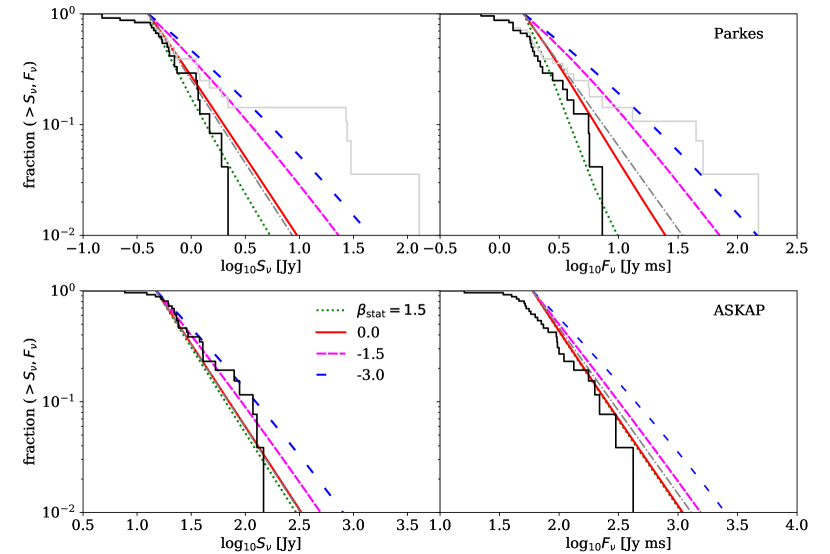
Figure 7: Left panels: the cumulative distribution of $S_{\nu}$. The results with ${\beta_{\rm stat}}=1.5$, 0.0, -1.5, and -3.0 are shown with dotted, solid, short-dashed, and long-dashed lines, respectively. The dot-dashed line indicates the power-law with index $\gamma=-1.5$, which is expected for objects homogeneously distributed in a Euclidean space. The black histograms show the distribution of the observed samples analyzed in this study, The gray histogram in the upper panel shows the distribution of the Parkes sample including the four outlier events that are excluded from our analysis (see Section 2). Right panels: same as the left panels but for $F_{\nu}$. The upper and lower panels show the distributions for the Parkes and ASKAP samples, respectively.

Figure 8: Upper pnaels: The power-low index $\gamma$ of the log$N$-log$S$ distribution of the Parkes samples, as derived by the maximum likelihood method (Crawford et al., 1970) as a function of the minimum $S_{\nu}$ ($F_{\nu}$) in the subsample used to derive $\gamma$. The errorbars represent the 90% confidence interval. The horizontal lines (dotted, solid, short-dashed, and long-dashed) represent the model predictions (${\beta_{\rm stat}}=1.5$, 0.0, -1.5, and -3.0, respectively). The gray datapoints are the results derived using subsamples with $\leq 10$ FRBs. The left and right panels show $\gamma$ for the $S_{\nu}$ and $F_{\nu}$ distributions, respectively. Lower panels: same as the upper panels but for the ASKAP sample.

Besides the log$N$–log$S$ distribution, the correlation between ${\rm DM_{EX}}$ and $S_{\nu}$ can be used as a clue to understand the nature of FRBs (Yang et al. 2017; N18; Shannon et al. 2018). Here we consider $S_{\nu}$ rather than $F_{\nu}$, because $S_{\nu}$ depends more strongly on distance than $F_{\nu}$ and hence the correlation with ${\rm DM_{EX}}$ becomes more significant. Distribution of FRBs on the parameter plane of ${\rm DM_{EX}}$ vs. $S_{\nu}$ assuming the best-fit parameters of the ${\rm DM_{EX}}$ distribution fitting is shown in Figure 9. Following N18, we randomly generate $10^{3}$ sets of mock samples of ${\rm DM_{EX}}$ and $S_{\nu}$ with sample size $N_{\rm sample}$ each in accordance with the model distributions, and compute probability distribution of the correlation coefficient between ${\rm DM_{EX}}$ and $S_{\nu}$. In figure 10, we show the mean and the standard deviation of the correlation coefficient distributions as functions of $N_{\rm sample}$.

Among the PL+E LF models, models with steeper faint-end shows weaker correlation between ${\rm DM_{EX}}$ and $S_{\nu}$, because more events are detected near the detection limit regardless of ${\rm DM_{EX}}$. When ${\beta_{\rm stat}}=1.5$, all the LF models predict weak correlation between ${\rm DM_{EX}}$ and $S_{\nu}$ for the ASKAP sample, because ${\rm DM_{host,med}}\sim 200$ cm^-3pc that is determined by the ${\rm DM_{EX}}$ distribution fitting occupies significant fraction of typical ${\rm DM_{EX}}\sim 350$ cm^-3pc of the ASKAP sample. However, the difference of the predictions between the models is difficult to distinguish with the current sample size (within $2\sigma$).

It should be also noted that a ${\rm DM_{EX}}$–$S_{\nu}$ correlation can be artificially produced by dispersion smearing which broadens pulse width (decreases $S_{\nu}$) more for FRBs with larger DM. However, as mentioned in N18, pulse width of the FRBs in the Parkes sample is not correlated with their ${\rm DM_{EX}}$ (correlation coefficient $=0.11$), suggesting that the ${\rm DM_{EX}}$–$S_{\nu}$ correlation is not primarily produced by dispersion smearing effect. On the other hand, pulse width of the FRBs in the ASKAP sample is correlated with ${\rm DM_{EX}}$ (correlation coefficient $=0.49$), and hence it is possible that the ${\rm DM_{EX}}$–$S_{\nu}$ correlation in the ASKAP sample is artificial. This is possibly due to the higher spectral resolution of the the Parkes sample ($\Delta\nu\sim 0.4$ MHz, Crawford et al., 2016) than the ASKAP sample ($\Delta\nu\sim 1$ MHz, Bannister et al., 2017).

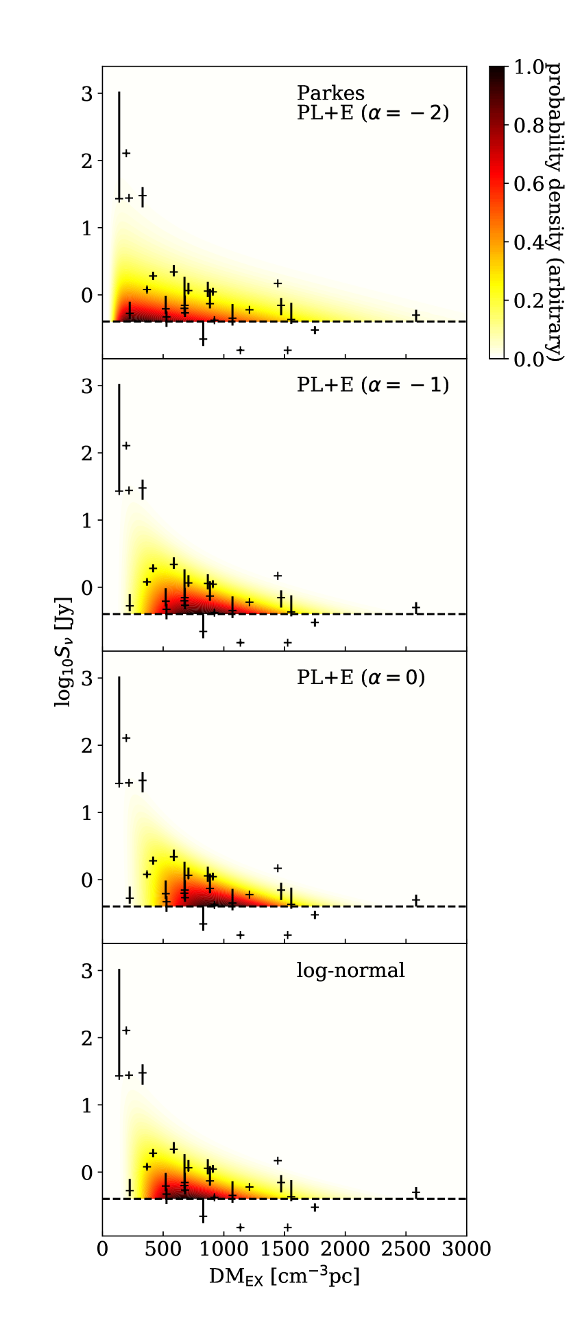
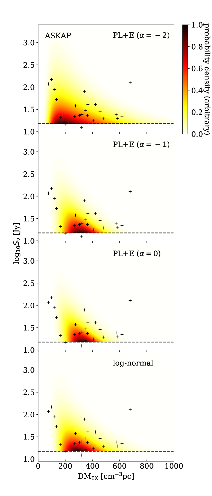
Figure 9: Left panels: probability distributions of FRBs on the parameter plane of ${\rm DM_{EX}}$ vs. $S_{\nu}$ predicted for the Parkes sample assuming ${\beta_{\rm stat}}=0.0$. The results with the PL+E LF models with $\alpha=-2.0,-1.0,0.0$, and the log-normal LF model are shown in the four panels from top to bottom. The datapoints are the observational data including the four outlier events that are excluded from the analysis ($S_{\nu}>10$ Jy, see Section 2). The horizontal dashed line in each panel indicates the assumed detection limit. Right panels: same as the left panels but for the ASKAP sample.

Figure 10: Left panels: mean and standard deviation of the correlation coefficient between ${\rm DM_{EX}}$ and $S_{\nu}$ generated by the Monte Carlo tests in accordance with the distribution functions shown in the left panels of figure 9 (models for the Parkes sample). The random generation of mock sample is performed 1000 times for each $N_{\rm sample}$. The results with ${\beta_{\rm stat}}=1.5$, 0.0, -1.5, and -3.0 are shown in the four panels from top to bottom. The datapoints connected with dashed, solid, dotted and dot-dashed lines show the correlation coefficient distribution with the PL+E LF models with $\alpha=-2.0,-1.0,0.0$, and the log-normal LF model, respectively. The result with the PL+E LF model with $\alpha=-2.0$ is not shown in the two panels from the bottom because the models do not have a solution in the ${\rm DM_{EX}}$ fitting. The data points are slightly shifted sideways for visibility. The horizontal double-dot-dashed line indicates the correlation coefficient between ${\rm DM_{EX}}$ and $S_{\nu}$ in the observed sample ($N_{\rm sample}=24$). Right panels: same as the left panels but for the ASKAP sample. The observed sample has $N_{\rm sample}=26$.

7 Conclusions

We have computed ${\rm DM_{EX}}$ distribution, log$N$-log$S$ distribution, and ${\rm DM_{EX}}$–$S_{\nu}$ correlation using an analytic model of FRB population that includes a variation of LF and $K$-correction models. FRB models that fulfill the following conditions are favored to reproduce the statistical properties of the Parkes and ASKAP samples of FRBs simultaneously,

1. DM components that are directly associated with FRB progenitors (CSM) are typically small ($<80$ cm^-3pc),

2. LF of FRBs has a bright-end cutoff at log${}_{10}L_{\nu}$ [erg s^-1Hz^-1] $\sim$ 34,

3. statistical effect of $K$-correction on observed flux density (or fluence) is smaller than a factor of 5 in the redshift range of $z\lesssim 2$ (i.e. $|{\beta_{\rm stat}}|<1.5$). In other words, the typical luminosity density of FRBs does not largely changed within the range of emitting frequency $\nu_{\rm rest}\sim$ 1–4 GHz.

although the statistical significance of the constraints are still low ($\sim 90$%) and larger sample of observed FRBs are necessary to obtain robust conclusions.

The conditions 1 & 2 are required to reproduce the ${\rm DM_{EX}}$ distributions of the Parkes and ASKAP samples simultaneously (§ 4.2). Although a larger DM component of $\gtrsim 100$ cm^-3pc can be associated with FRB progenitors if there is a strong negative $K$-correction effect (${\beta_{\rm stat}}\sim 1.5$). However, models with $|{\beta_{\rm stat}}|>1.5$ are disfavored by the observed log$N$–log$S$ distribution of the Parkes sample (condition 3, § 6).

The constraint on ${\rm DM_{host,med}}$ obtained by our analysis indicates that major part of ${\rm DM_{EX}}$ of an FRB indeed arise from the IGM and is a good indicator of distance, that will help us to understand FRBs in terms of their distance distribution and energetics. Together with more robust test of the results shown here by larger sample size and redshift measurements of FRBs, FRBs will also provide us with an unprecedented opportunity to study the IGM observationally.

References

- Bannister et al. (2017) Bannister, K. W., Shannon, R. M., Macquart, J. P., et al. 2017, ApJ, 841, L12, doi: 10.3847/2041-8213/aa71ff
- Bannister et al. (2019) Bannister, K. W., Deller, A. T., Phillips, C., et al. 2019, Science, 365, 565, doi: 10.1126/science.aaw5903
- Bhandari et al. (2018) Bhandari, S., Keane, E. F., Barr, E. D., et al. 2018, MNRAS, 475, 1427, doi: 10.1093/mnras/stx3074
- Bochenek et al. (2020) Bochenek, C. D., Ravi, V., Belov, K. V., et al. 2020, arXiv e-prints, arXiv:2005.10828. https://arxiv.org/abs/2005.10828
- Caleb et al. (2016) Caleb, M., Flynn, C., Bailes, M., et al. 2016, MNRAS, 458, 708, doi: 10.1093/mnras/stw175
- Cordes & Lazio (2002) Cordes, J. M., & Lazio, T. J. W. 2002, ArXiv Astrophysics e-prints
- Cordes & Wasserman (2016) Cordes, J. M., & Wasserman, I. 2016, MNRAS, 457, 232, doi: 10.1093/mnras/stv2948
- Cordes et al. (2017) Cordes, J. M., Wasserman, I., Hessels, J. W. T., et al. 2017, ApJ, 842, 35, doi: 10.3847/1538-4357/aa74da
- Cordes et al. (2016) Cordes, J. M., Wharton, R. S., Spitler, L. G., Chatterjee, S., & Wasserman, I. 2016, ArXiv e-prints. https://arxiv.org/abs/1605.05890
- Crawford et al. (1970) Crawford, D. F., Jauncey, D. L., & Murdoch, H. S. 1970, ApJ, 162, 405, doi: 10.1086/150672
- Crawford et al. (2016) Crawford, F., Rane, A., Tran, L., et al. 2016, MNRAS, 460, 3370, doi: 10.1093/mnras/stw1233
- DeLaunay et al. (2016) DeLaunay, J. J., Fox, D. B., Murase, K., et al. 2016, ApJ, 832, L1, doi: 10.3847/2041-8205/832/1/L1
- Dolag et al. (2015) Dolag, K., Gaensler, B. M., Beck, A. M., & Beck, M. C. 2015, MNRAS, 451, 4277, doi: 10.1093/mnras/stv1190
- Falcke & Rezzolla (2014) Falcke, H., & Rezzolla, L. 2014, A&A, 562, A137, doi: 10.1051/0004-6361/201321996
- Hassall et al. (2013) Hassall, T. E., Keane, E. F., & Fender, R. P. 2013, MNRAS, 436, 371, doi: 10.1093/mnras/stt1598
- Inoue (2004) Inoue, S. 2004, MNRAS, 348, 999, doi: 10.1111/j.1365-2966.2004.07359.x
- Ioka (2003) Ioka, K. 2003, ApJ, 598, L79, doi: 10.1086/380598
- Kashiyama et al. (2013) Kashiyama, K., Ioka, K., & Mészáros, P. 2013, ApJ, 776, L39, doi: 10.1088/2041-8205/776/2/L39
- Katz (2016) Katz, J. I. 2016, ApJ, 818, 19, doi: 10.3847/0004-637X/818/1/19
- Keane & Petroff (2015) Keane, E. F., & Petroff, E. 2015, MNRAS, 447, 2852, doi: 10.1093/mnras/stu2650
- Keane et al. (2012) Keane, E. F., Stappers, B. W., Kramer, M., & Lyne, A. G. 2012, MNRAS, 425, L71, doi: 10.1111/j.1745-3933.2012.01306.x
- Keane et al. (2016) Keane, E. F., Johnston, S., Bhandari, S., et al. 2016, Nature, 530, 453, doi: 10.1038/nature17140
- Kokubo et al. (2017) Kokubo, M., Mitsuda, K., Sugai, H., et al. 2017, ApJ, 844, 95, doi: 10.3847/1538-4357/aa7b2d
- Lorimer et al. (2007) Lorimer, D. R., Bailes, M., McLaughlin, M. A., Narkevic, D. J., & Crawford, F. 2007, Science, 318, 777, doi: 10.1126/science.1147532
- Lu et al. (2020) Lu, W., Kumar, P., & Zhang, B. 2020, arXiv e-prints, arXiv:2005.06736. https://arxiv.org/abs/2005.06736
- Lu & Piro (2019) Lu, W., & Piro, A. L. 2019, ApJ, 883, 40, doi: 10.3847/1538-4357/ab3796
- Luo et al. (2018) Luo, R., Lee, K., Lorimer, D. R., & Zhang, B. 2018, MNRAS, 481, 2320, doi: 10.1093/mnras/sty2364
- Luo et al. (2020) Luo, R., Men, Y., Lee, K., et al. 2020, MNRAS, 494, 665, doi: 10.1093/mnras/staa704
- Macquart & Ekers (2018) Macquart, J.-P., & Ekers, R. D. 2018, MNRAS, 474, 1900, doi: 10.1093/mnras/stx2825
- Madau & Dickinson (2014) Madau, P., & Dickinson, M. 2014, ARA&A, 52, 415, doi: 10.1146/annurev-astro-081811-125615
- Marcote et al. (2020) Marcote, B., Nimmo, K., Hessels, J. W. T., et al. 2020, Nature, 577, 190, doi: 10.1038/s41586-019-1866-z
- Margalit et al. (2020) Margalit, B., Beniamini, P., Sridhar, N., & Metzger, B. D. 2020, arXiv e-prints, arXiv:2005.05283. https://arxiv.org/abs/2005.05283
- Niino (2018) Niino, Y. 2018, ApJ, 858, 4 (N18), doi: 10.3847/1538-4357/aab9a9
- Niino et al. (2018) Niino, Y., Tominaga, N., Totani, T., et al. 2018, PASJ, 70, L7, doi: 10.1093/pasj/psy102
- Palaniswamy et al. (2018) Palaniswamy, D., Li, Y., & Zhang, B. 2018, ApJ, 854, L12, doi: 10.3847/2041-8213/aaaa63
- Petroff et al. (2015) Petroff, E., Bailes, M., Barr, E. D., et al. 2015, MNRAS, 447, 246, doi: 10.1093/mnras/stu2419
- Petroff et al. (2016) Petroff, E., Barr, E. D., Jameson, A., et al. 2016, PASA, 33, e045, doi: 10.1017/pasa.2016.35
- Piro & Burke-Spolaor (2017) Piro, A. L., & Burke-Spolaor, S. 2017, ApJ, 841, L30, doi: 10.3847/2041-8213/aa740d
- Platts et al. (2019) Platts, E., Weltman, A., Walters, A., et al. 2019, Phys. Rep., 821, 1, doi: 10.1016/j.physrep.2019.06.003
- Popov & Postnov (2013) Popov, S. B., & Postnov, K. A. 2013, ArXiv e-prints. https://arxiv.org/abs/1307.4924
- Prochaska & Zheng (2019) Prochaska, J. X., & Zheng, Y. 2019, MNRAS, 485, 648, doi: 10.1093/mnras/stz261
- Prochaska et al. (2019) Prochaska, J. X., Macquart, J.-P., McQuinn, M., et al. 2019, Science, 366, 231, doi: 10.1126/science.aay0073
- Ravi et al. (2019) Ravi, V., Catha, M., D’Addario, L., et al. 2019, Nature, 572, 352, doi: 10.1038/s41586-019-1389-7
- Shannon et al. (2018) Shannon, R. M., Macquart, J. P., Bannister, K. W., et al. 2018, Nature, 562, 386, doi: 10.1038/s41586-018-0588-y
- Staveley-Smith et al. (1996) Staveley-Smith, L., Wilson, W. E., Bird, T. S., et al. 1996, PASA, 13, 243
- Tendulkar et al. (2017) Tendulkar, S. P., Bassa, C. G., Cordes, J. M., et al. 2017, ApJ, 834, L7, doi: 10.3847/2041-8213/834/2/L7
- The CHIME/FRB Collaboration (2020) The CHIME/FRB Collaboration, :, Andersen, B. C., et al. 2020, arXiv e-prints, arXiv:2005.10324. https://arxiv.org/abs/2005.10324
- Thornton et al. (2013) Thornton, D., Stappers, B., Bailes, M., et al. 2013, Science, 341, 53, doi: 10.1126/science.1236789
- Tominaga et al. (2018) Tominaga, N., Niino, Y., Totani, T., et al. 2018, PASJ, 70, 103, doi: 10.1093/pasj/psy101
- Totani (2013) Totani, T. 2013, PASJ, 65, L12, doi: 10.1093/pasj/65.5.L12
- Walker et al. (2018) Walker, C. R. H., Ma, Y. Z., & Breton, R. P. 2018, arXiv e-prints, arXiv:1804.01548. https://arxiv.org/abs/1804.01548
- Xu & Han (2015) Xu, J., & Han, J. L. 2015, Research in Astronomy and Astrophysics, 15, 1629, doi: 10.1088/1674-4527/15/10/002
- Yamasaki & Totani (2020) Yamasaki, S., & Totani, T. 2020, ApJ, 888, 105, doi: 10.3847/1538-4357/ab58c4
- Yang et al. (2017) Yang, Y.-P., Luo, R., Li, Z., & Zhang, B. 2017, ApJ, 839, L25, doi: 10.3847/2041-8213/aa6c2e
- Zhang (2017) Zhang, B. 2017, ApJ, 836, L32, doi: 10.3847/2041-8213/aa5ded